Reality conditions for the KdV equation
and quasi-periodic solutions in finite phase spaces

Abstract.

In this paper reality conditions for finite-gap solutions of the KdV equation are determined. This new result brings the last piece of the puzzle of obtaining quasi-periodic solutions of completely integrable dynamical equations. Effective computation of the solutions is suggested, and illustrated in genera $2$ and $3$.

Real-valued quasi-periodic solutions, which describe nonlinear waves, are proposed in every finite phase space of the hierarchy of hamiltonian systems of the KdV equation. These solutions are expressed in terms of the abelian $\wp_{1,1}$-function, which comes as a result of algebro-geometric integration. The construction of the hierarchy on coadjoint orbits of an $\mathrm{SL}(2,\operatorname{\mathbb{R}})$ loop group is also addressed.

1. Introduction

The Korteweg—de Vries equation (KdV) arose in the $19$th century in connection with the theory of waves in shallow water, see [16]. It is known that this equation also describes the propagation of waves with weak dispersion in various nonlinear media, see [15]. The conventional form of KdV is

(1) $$w_{t}=6ww_{x}+w_{xxx}.$$

This equation is scale-invariant, that is multiplying $t$, $x$, and $w$ by constants can be used to make the coefficients of any of the three terms equal to any given non-zero constants.

First known solutions: the one-soliton solution and the simplest non-linear wave solution — were suggested by Korteweg and de Vries in [16].

In [13] a remarkable procedure of finding soliton solutions of KdV, known as the inverse scattering method, was discovered. Soon, it was shown that the KdV equation admits the Lax representation [19], and possesses a sequence of integrals of motion [21], which tends to be infinite. Further, in [11], it was proven, that the sequence of integrals of motion of KdV is infinite, and so KdV was called a completely integrable hierarchy of hamiltonian systems. In [22] the notion of a finite-gap solution of KdV arose; such a solution lives within a hamiltonian system of a fixed dimension. Also the higher KdV equations were introduced in [22].

Wide variety of integrable equations on orbits of coadjoint representations of finite Lie groups was introduced in [20, 12]. A further development of the orbit approach was given in [1, 2, 17]

The paper is organized as follows. In Preliminaries we recall all notions related to uniformization of hyperelliptic curves: the standard not normalized differentials of the first kind and associated to them differentials of the second kind, Abel’s map, theta and sigma functions, the Jacobi inversion problem, and also briefly explain the construction of hamiltonian systems on coadjoint orbits of a loop group. In section 3 hamiltonian systems which constitute the KdV hierarchy are developed. Section 4 is devoted to separation of variables. In section 5 the algebro-geometric integration is explained in application to the KdV hierarchy. Finally, section 6 presents new results on finding real-valued quasi-periodic solutions of the KdV equation in any finite phase space. Section 7 illustrates an effective computation of the quasi-periodic solutions in genera $1$, $2$, and $3$.

2. Preliminaries

2.1. Hyperelliptic curves

Let a non-degenerate hyperelliptic curve $\mathcal{V}$ of genus $g$ be defined by

(2) $$-y^{2}+z^{2g+1}+\sum_{i=1}^{2g}\lambda_{2i+2}z^{2g-i}=0.$$

Let $(e_{i},0)$, $i=1$, …, $2g+1$, be finite branch points of the curve (2). In what follows, we denote branch points simply by $e_{i}$. Homology basis is defined after H. Baker [3, § 200]. One can imagine a continuous path through all branch points, which starts at infinity and ends at infinity, see the orange line on fig. 1.

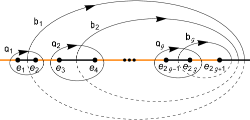
Figure 1. Cuts and cycles on a hyperelliptic curve.

The branch points are enumerated along the path. Fig. 1 represents the case of all real branch points, on which the present paper focuses. Cuts are made between points $e_{2k-1}$ and $e_{2k}$ with $k$ from $1$ to $g$. One more cut starts at $e_{2g+1}$ and ends at infinity. Canonical homology cycles are defined as follows. Each $\mathfrak{a}_{k}$-cycle encircles the cut $(e_{2k-1},e_{2k})$, $k=1$, …$g$, and each $\mathfrak{b}_{k}$-cycle emerges from the cut $(e_{2k-1},e_{2k})$ and enters the cut $(e_{2g+1},\infty)$, see fig. 1.

Let $\mathrm{d}u=(\mathrm{d}u_{1},\mathrm{d}u_{3},\dots,\mathrm{d}u_{2g-1})^{t}$ be not normalized differentials of the first kind, and $\mathrm{d}r=(\mathrm{d}r_{1},\mathrm{d}r_{3},\dots,\mathrm{d}r_{2g-1})^{t}$ be differentials of the second kind associated with the first kind differentials, see [3, § 138] for more detail. Actually,

(3a) $$\mathrm{d}u_{2n-1}=\frac{z^{g-n}\mathrm{d}z}{\partial_{y}f(z,y)},\quad n=1,\dots,g,$$

(3b) $$\mathrm{d}r_{2n-1}=\frac{\mathrm{d}z}{\partial_{y}f(z,y)}\bigg{(}z^{g+n-1}+\sum_{j=1}^{2n-2}(2n-1-j)\lambda_{2j}z^{g+n-1-j}\bigg{)},$$

where $\partial_{w}f(z,y)=-2y$. The indices of $\mathrm{d}u_{2n-1}$ display the orders of zeros, and the indices of $\mathrm{d}r_{2n-1}$ display the orders of poles.

Let not nomalized periods along the canonical cycles $\mathfrak{a}_{k}$, $\mathfrak{b}_{k}$, $k=1$, …, $g$, be defined as follows

$$\omega_{k}=\oint_{\mathfrak{a}_{k}}\mathrm{d}u,\qquad\qquad\omega^{\prime}_{k}=\oint_{\mathfrak{b}_{k}}\mathrm{d}u.$$

The vectors $\omega_{k}$, $\omega^{\prime}_{k}$ form first kind period matrices $\omega$, $\omega^{\prime}$, respectively.

The corresponding normalized period matrices are $1_{g}$, $\tau$, where $1_{g}$ denotes the identity matrix of size $g$, and $\tau=\omega^{-1}\omega^{\prime}$. Matrix $\tau$ is symmetric with a positive imaginary part: $\tau^{t}=\tau$, $\operatorname{\mathrm{Im}}\tau>0$, that is $\tau$ belongs to the Siegel upper half-space. The normalized holomorphic differentials are denoted by

$$\mathrm{d}v=\omega^{-1}\mathrm{d}u.$$

2.2. Abel’s map

The vectors $\omega_{k}$, $\omega^{\prime}_{k}$ serve as generators of a period lattice $\mathfrak{P}$. Then $\operatorname{\mathfrak{J}}=\operatorname{\mathbb{C}}^{g}/\mathfrak{P}$ is the Jacobian variety of the curve (2). Let $u=(u_{1},u_{3},\dots,u_{2g-1})^{t}$ be a point of $\operatorname{\mathfrak{J}}$.

Let the Abel map be defined by

$$\mathcal{A}(P)=\int_{\infty}^{P}\mathrm{d}u,\qquad P=(z,y)\in\mathcal{V}.$$

The Abel map of a positive divisor $D=\sum_{i=1}^{n}(z_{i},y_{i})$ is defined by

$$\mathcal{A}(D)=\sum_{i=1}^{n}\int_{\infty}^{(z_{i},y_{i})}\mathrm{d}u.$$

The map is one-to-one on the $g$-th symmetric power of the curve: $\mathcal{A}:\mathcal{V}^{g}\mapsto\operatorname{\mathfrak{J}}$.

2.3. Jacobi inversion problem

A solution of the Jacobi inversion problem on a hyperelliptic curve is proposed in [3, Art. 216], see also [7, Theorem 2.2]. Let $u=\mathcal{A}(D)$ be the Abel image of a non-special positive divisor $D\in\mathcal{V}^{g}$. Then $D$ is uniquely defined by the system of equations

(4a) $$\mathcal{R}_{2g}(z,y;u)\equiv z^{g}-\sum_{i=1}^{g}z^{g-i}\wp_{1,2i-1}(u)=0,$$

(4b) $$\mathcal{R}_{2g+1}(z,y;u)\equiv 2y+\sum_{i=1}^{g}z^{g-i}\wp_{1,1,2i-1}(u)=0.$$

2.4. Theta function

The Riemann theta function is defined by

$$\theta(v;\tau)=\sum_{n\in\operatorname{\mathbb{Z}}^{g}}\exp\big{(}\imath\pi n^{t}\tau n+2\imath\pi n^{t}v\big{)}.$$

This function is supposed to be related to the curve (2), it depends on the normalized coordinates $v=\omega^{-1}u$, $u\in\operatorname{\mathfrak{J}}$, and periods $\tau=\omega^{-1}\omega^{\prime}$. Let

$$\theta[\varepsilon](v;\tau)=\exp\big{(}\imath\pi(\varepsilon^{\prime}{}^{t}/2)\tau(\varepsilon^{\prime}/2)+2\imath\pi(v+\varepsilon/2)^{t}\varepsilon^{\prime}/2\big{)}\times\\ \times\theta(v+\varepsilon/2+\tau\varepsilon^{\prime}/2;\tau)$$

be the theta function with characteristic $[\varepsilon]=(\varepsilon^{\prime},\varepsilon)^{t}$. A characteristic $[\varepsilon]$ is a $2\times g$ matrix, all components of $\varepsilon$, and $\varepsilon^{\prime}$ are real values within the interval $[0,2)$. Modulo ($\operatorname{mod}$) $2$ addition is defined on characteristics.

Every point $u$ within a fundamental domain of the Jacobian variety $\operatorname{\mathfrak{J}}$ can be represented by its characteristic $[\varepsilon]$ defined as follows

$$u=\tfrac{1}{2}\omega\varepsilon+\tfrac{1}{2}\omega^{\prime}\varepsilon^{\prime}.$$

Abel’s images of branch points are described by characteristics with integer components, as well as Abel’s image of any combination of branch points. An integer characteristic $[\varepsilon]$ is odd whenever $\varepsilon^{t}\varepsilon^{\prime}=0$ ($\operatorname{mod}2$), and even whenever $\varepsilon^{t}\varepsilon^{\prime}=1$ ($\operatorname{mod}2$). A theta function with characteristic has the same parity as its characteristic.

2.5. Sigma function

The modular invariant entire function on $\operatorname{\mathfrak{J}}$ is called the sigma function. In the present paper we define it by the relation with the theta function:

(5) $$\sigma(u)=C\exp\big{(}{-}\tfrac{1}{2}u^{t}\varkappa u\big{)}\theta[K](\omega^{-1}u;\omega^{-1}\omega^{\prime}).$$

Note, that the sigma function is defined in terms of not normalized coordinates $u$, and associated with not normalized period matrices of the first kind $\omega$, $\omega^{\prime}$, and of the second kind $\eta$, $\eta^{\prime}$. The latter matrices are formed by the vectors

$$\eta_{k}=\oint_{\mathfrak{a}_{k}}\mathrm{d}r,\qquad\qquad\eta^{\prime}_{k}=\oint_{\mathfrak{b}_{k}}\mathrm{d}r,$$

respectively. Then $\varkappa=\eta\omega^{-1}$ is a symmetric matrix.

In what follows we use multiply periodic $\wp$-functions

$$\wp_{i,j}(u)=-\frac{\partial^{2}\log\sigma(u)}{\partial u_{i}\partial u_{j}},\qquad\wp_{i,j,k}(u)=-\frac{\partial^{3}\log\sigma(u)}{\partial u_{i}\partial u_{j}\partial u_{k}}.$$

For constructing series representation of the sigma function see [10].

2.6. Characteristics and partitions

Let $\mathcal{S}=\{0,1,2,\dots,2g+1\}$ be the set of indices of all branch points of a hyperellipitic curve of genus $g$, and $0$ stands for the branch point at infinity. According to [3, § 202] all half-period characteristics are represented by partitions of $\mathcal{S}$ of the form $\mathcal{I}_{\mathfrak{m}}\cup\mathcal{J}_{\mathfrak{m}}$ with $\mathcal{I}_{\mathfrak{m}}=\{i_{1},\,\dots,\,i_{g+1-2\mathfrak{m}}\}$ and $\mathcal{J}_{\mathfrak{m}}=\{j_{1},\,\dots,\,j_{g+1+2\mathfrak{m}}\}$, where $\mathfrak{m}$ runs from $0$ to $[(g+1)/2]$, and $[\cdot]$ denotes the integer part. Index $0$, corresponding to infinity, is usually omitted in sets, it is also omitted in computation of cardinality of a set.

Denote by $[\varepsilon(\mathcal{I})]=\sum_{i\in\mathcal{I}}[\varepsilon_{i}]$ $(\operatorname{mod}2)$ the characteristic of

$$\mathcal{A}(\mathcal{I})=\sum_{i\in\mathcal{I}}\mathcal{A}(e_{i})=\omega\Big{(}\frac{1}{2}\varepsilon(\mathcal{I})+\frac{1}{2}\tau\varepsilon^{\prime}(\mathcal{I})\Big{)}.$$

Characteristics of $2g+1$ branch points serve as a basis for constructing all $2^{2g}$ half-period characteristics. Below a partition is referred to by the part of less cardinality, denoted by $\mathcal{I}$.

Introduce also characteristic

$$[\mathcal{I}]=[\varepsilon(\mathcal{I})]+[K]$$

of $\mathcal{A}(\mathcal{I})+K$, where $K$ denotes the vector of Riemann constants. Characteristic $[K]$ of the vector of Riemann constants equals the sum of all odd characteristics of branch points, there are $g$ such characteristics, see [3, § 200, 202]. In the basis of canonical cycles introduced by fig. 1 we have

$$[K]=\sum_{k=1}^{g}[\varepsilon_{2k}].$$

Let $\mathcal{I}_{\mathfrak{m}}\cup\mathcal{J}_{\mathfrak{m}}$ be a partition introduced above, then $[\mathcal{I}_{\mathfrak{m}}]=[\mathcal{J}_{\mathfrak{m}}]$. Characteristics $[\mathcal{I}_{\mathfrak{m}}]$ of even multiplicity $\mathfrak{m}$ are even, and of odd $\mathfrak{m}$ are odd. According to the Riemann vanishing theorem, $\theta(v+\mathcal{A}(\mathcal{I}_{\mathfrak{m}})+K;\tau)$ vanishes to order $\mathfrak{m}$ at $v\,{=}\,0$. Number $\mathfrak{m}$ is called multiplicity. Characteristics of multiplicity $0$ are called non-singular even characteristics. Characteristics of multiplicity $1$ are called non-singular odd. All other characteristics are called singular.

2.7. Hamiltonian systems on coadjoint orbits

Let $\mathfrak{g}$ be a semi-simple Lie algebra, and $\mathfrak{g}^{\ast}$ be the dual algebra to $\mathfrak{g}$ with respect to a bilinear form $\langle\cdot,\cdot\rangle:\mathfrak{g}^{\ast}\times\mathfrak{g}\mapsto\operatorname{\mathbb{C}}$. That is, $\mathfrak{g}^{\ast}$ is the space of $1$-forms $\Psi$ on $\mathfrak{g}$.

An orbit of coadjoint action of the corresponding Lie group $G=\exp(\mathfrak{g})$ is defined by

$$\mathcal{O}=\{\Psi\mid\Psi=\operatorname{Ad}^{\ast}_{g}\Phi,\ g\in G\},$$

where $\Phi$ denote an initial point in $\mathfrak{g}^{\ast}$. If $S$ is the stationary subgroup of $\Phi$ in $G$, then

$$\mathcal{O}=G/S.$$

The tangent space at $\Psi\in\mathcal{O}$ is

$$T_{\Psi}=\{\operatorname{ad}_{A}^{\ast}\Psi\mid A\in\mathfrak{g}\},$$

where $\operatorname{ad}_{A}^{\ast}\Psi=-\operatorname{ad}_{A}\Psi=[\Psi,A]$. If $A\in\mathfrak{s}_{\Psi}$, where $\exp(\mathfrak{s}_{\Psi})=S_{\Psi}$ is the stationary subgroup of $\Psi$, then $\operatorname{ad}_{A}^{\ast}\Psi=0$. Thus,

$$T_{\Psi}=\mathfrak{g}/\mathfrak{s}_{\Psi}.$$

When $\Psi$ runs the orbit $\mathcal{O}$, and $A\in\mathfrak{g}/\mathfrak{s}_{\Psi}$ is fixed, tangent vectors $\operatorname{ad}_{A}^{\ast}\Psi$ draw a vector field $\widetilde{A}$ on the orbit. Denote by $\rho$ the map $A\mapsto\widetilde{A}$. Let

$$T(\mathcal{O})=\{\widetilde{A}\overset{\rho}{=}\operatorname{ad}_{A}^{\ast}\Psi\mid A\in\mathfrak{g}/\mathfrak{s}_{\Psi},\Psi\in\mathcal{O}\}$$

be the tangent space of the orbit $\mathcal{O}$.

At a point $\Psi\in\mathfrak{g}^{\ast}$ a skew-symmetric $2$-form $\varpi_{\Psi}:T(\mathcal{O})\times T(\mathcal{O})\mapsto\operatorname{\mathbb{C}}$ is defined by the rule

(6) $$\varpi_{\Psi}(\widetilde{A},\widetilde{B})=\langle\Psi,[A,B]\rangle.$$

The form $\varpi_{\Psi}$ is non-degenerate and closed, that follows immediately from the definition (6). The form $\varpi$ is $G$-invariant: that is, it does not change when $\Psi$ runs the orbit, since vector fields $\widetilde{A}$, $\widetilde{B}$ transform in accordance with $\Psi$, namely $\widetilde{A}\overset{\rho}{=}\operatorname{ad}_{A}^{\ast}\Psi$, $\widetilde{B}\overset{\rho}{=}\operatorname{ad}_{B}^{\ast}\Psi$.

An orbit $\mathcal{O}$ equipped with a non-degenerate closed $2$-form (6) serves as a homogeneous symplectic manifold. The form $\varpi$ realizes the isomorphism between the space of $1$-forms $\mathfrak{g}^{\ast}$ and the space of vector fields $T(\mathcal{O})$. Below we explain this in more detail.

Let $X_{i}$ form a basis of $\mathfrak{g}$, and $\Xi_{i}$ form the dual basis of $\mathfrak{g}^{\ast}$ such that $\langle\Xi_{i},X_{j}\rangle=\delta_{i,j}$, where $\delta_{i,j}$ is the Kronecker delta. Then $\langle\Psi,X_{i}\rangle=\psi_{i}$ serve as coordinates of $\Psi\in\mathfrak{g}^{\ast}$ in the chosen basis. Let $\mathcal{C}(\mathfrak{g}^{\ast})$ be the space of smooth functions on $\mathfrak{g}^{\ast}$. Let $B(\mathfrak{g}^{\ast},\mathfrak{g})$ be the space of closed $1$-forms $\nabla\mathcal{F}$ assigned to $\mathcal{F}\in\mathcal{C}(\mathfrak{g}^{\ast})$ by the rule

$$\nabla\mathcal{F}(\Psi)=\sum_{i}\frac{\partial\mathcal{F}(\Psi)}{\partial\psi_{i}}X_{i}.$$

On the other hand, every $X\in\mathfrak{g}/\mathfrak{s}_{\Psi}$ gives rise to a vector field $\widetilde{X}\overset{\rho}{=}\operatorname{ad}^{\ast}_{X}\Psi$, tangent to $\mathcal{O}\subset\mathfrak{g}^{\ast}$. Therefore, we have

$$\mathcal{C}(\mathfrak{g}^{\ast})\to B(\mathfrak{g}^{\ast},\mathfrak{g})\overset{\rho}{\to}T(\mathcal{O}),$$

$$\mathcal{F}(\Psi)\mapsto\nabla\mathcal{F}(\Psi)\mapsto\operatorname{ad}^{\ast}_{\nabla\mathcal{F}(\Psi)}\Psi.$$

This defines the isomorphism between $1$-forms and vector fields.

The map $\rho$ is defined on all $1$-forms $\sum_{i}\mathcal{F}_{i}X_{i}\in\mathfrak{g}$. The inverse map brings $\operatorname{ad}^{\ast}_{X(\Psi)}\Psi$ to $1$-form $\Xi_{\Psi}$ which acts on another vector field $\operatorname{ad}^{\ast}_{A}\Psi$ as follows

$$\Xi_{\Psi}(\operatorname{ad}^{\ast}_{A}\Psi)=\langle\Psi,[X(\Psi),A]\rangle.$$

In what follows, we call a function $\mathcal{F}\in\mathcal{C}(\mathfrak{g}^{\ast})$ a hamiltonian, and $\operatorname{ad}^{\ast}_{\nabla\mathcal{F}(\Psi)}\Psi$ the corresponding hamiltonian vector field. In particular, $\psi_{i}=\langle\Psi,X_{i}\rangle$ serve as hamiltonians of the vector fields $\operatorname{ad}^{\ast}_{X_{i}}\Psi$. A commutator of two hamiltonian vector fields is a hamiltonian vector field, which is defined through the Lie—Poisson bracket:

(7) $$\begin{split}\{\mathcal{F},\mathcal{H}\}&=\langle\Psi,\bigg{[}\sum_{i}\frac{\partial\mathcal{F}(\Psi)}{\partial\psi_{i}}X_{i},\sum_{j}\frac{\partial\mathcal{H}(\Psi)}{\partial\psi_{j}}X_{j}\bigg{]}\rangle\\ &=\sum_{i,j}\frac{\partial\mathcal{F}(\Psi)}{\partial\psi_{i}}\frac{\partial\mathcal{H}(\Psi)}{\partial\psi_{j}}\langle\Psi,[X_{i},X_{j}]\rangle.\end{split}$$

Every hamiltonian $\mathcal{H}$ gives rise to a flow

$$\frac{\mathrm{d}\Psi}{\mathrm{d}\tau}=\operatorname{ad}^{\ast}_{\nabla\mathcal{H}}\Psi,$$

or in coordinates

$$\frac{\mathrm{d}\psi_{i}}{\mathrm{d}\tau}=\langle\operatorname{ad}^{\ast}_{\nabla\mathcal{H}}\Psi,X_{i}\rangle=\{\mathcal{H},\psi_{i}\},$$

which is a system of hamiltonian equations, and $\tau$ serves as a parameter along the hamiltonian vector field. The fact that $X_{i}\in\mathfrak{g}/\mathfrak{s}_{\Psi}$ is not essential, since $\operatorname{ad}^{\ast}_{X_{i}}\Psi=0$ if $X_{i}\in\mathfrak{s}_{\Psi}$.

3. Integrable systems on coadjoint orbits of a loop group

The KdV equation arises within the hierarchy of integrable Hamiltonian systems on coadjoint orbits of loop $\mathrm{SL}(2,\operatorname{\mathbb{R}})$-group. Here we briefly recall this scheme, as presented in [14] and recalled in [6]. Such a construction is based on the results of [1, 2].

Let $\widetilde{\mathfrak{g}}=\mathfrak{g}\otimes\mathcal{P}(z,z^{-1})$, where $\mathcal{P}(z,z^{-1})$ denotes the algebra of Laurent series in $z$, and $\mathfrak{g}=\mathfrak{sl}(2,\operatorname{\mathbb{C}})$ has the standard basis

$$H=\frac{1}{2}\begin{pmatrix}1&0\\ 0&-1\end{pmatrix},\quad X=\begin{pmatrix}0&1\\ 0&0\end{pmatrix},\quad Y=\begin{pmatrix}0&0\\ 1&0\end{pmatrix}.$$

In the algebra $\widetilde{\mathfrak{g}}$ the principal grading is introduced, defined by the grading operator

$$\mathfrak{d}=2z\frac{\mathrm{d}}{\mathrm{d}z}+\operatorname{ad}_{H},$$

where $\operatorname{ad}$ denotes the adjoint operator in $\mathfrak{g}$, that is $\forall X\in\mathfrak{g}$ $\operatorname{ad}_{H}X=[H,X]$.

Let $\{X_{2m-1},\,Y_{2m-1},\,H_{2m},\mid m\in\operatorname{\mathbb{Z}}\}$, such that

$$X_{2m-1}=z^{m-1}X,\quad Y_{2m-1}=z^{m}Y,\quad H_{2m}=z^{m}H,$$

form a basis of $\widetilde{\mathfrak{g}}$. In general, an element of the basis will be denoted by $Z_{a,\ell}$, where $a=1$, $2$, $3$, and $\ell$ indicates the degree of $Z_{a,\ell}$, namely $\mathfrak{d}Z_{a,\ell}=\ell Z_{a,\ell}$. Actually, $Z_{1,\ell}=H_{\ell}$, $Z_{2,\ell}=Y_{\ell}$, $Z_{3,\ell}=X_{\ell}$. Let $\mathfrak{g}_{\ell}$ denote the degree $\ell$ eigenspace of $\mathfrak{d}$. Thus, $\mathfrak{g}_{2m-1}=\operatorname{span}\{X_{2m-1},\,Y_{2m-1}\}$, and $\mathfrak{g}_{2m}=\operatorname{span}\{H_{2m}\}$.

According to the scheme from [2], $\widetilde{\mathfrak{g}}$ is divided into two subalgebras

$$\widetilde{\mathfrak{g}}_{+}=\oplus\sum_{\ell\geqslant 0}\mathfrak{g}_{\ell},\qquad\widetilde{\mathfrak{g}}_{-}=\oplus\sum_{\ell<0}\mathfrak{g}_{\ell}.$$

The bilinear form

$$\forall A(z),B(z)\in\widetilde{\mathfrak{g}}\qquad\langle A(z),B(z)\rangle=\operatorname*{res}_{z=0}\operatorname{tr}A(z)B(z)$$

introduces the duality

$$X_{2m-1}^{\ast}\leftrightarrow X_{-2m-1},\quad Y_{2m-1}^{\ast}\leftrightarrow Y_{-2m-1},\quad H_{2m}^{\ast}\leftrightarrow H_{-2m-2},$$

where $\{X_{2m-1}^{\ast},\,Y_{2m-1}^{\ast},\,H_{2m}^{\ast},\mid m\in\operatorname{\mathbb{Z}}\}$, such that

$$X_{2m-1}^{\ast}=z^{m}X^{\ast},\quad Y_{2m-1}^{\ast}=z^{m-1}Y^{\ast},\quad H_{2m}^{\ast}=z^{m}H^{\ast},$$

form the basis of $\widetilde{\mathfrak{g}}^{\ast}$, and the basis elements of $\mathfrak{g}^{\ast}$ are

$$H^{\ast}=\begin{pmatrix}1&0\\ 0&-1\end{pmatrix},\quad X^{\ast}=\begin{pmatrix}0&0\\ 1&0\end{pmatrix},\quad Y^{\ast}=\begin{pmatrix}0&1\\ 0&0\end{pmatrix}.$$

Then the dual subalgebras $\widetilde{\mathfrak{g}}_{+}^{\ast}$ and $\widetilde{\mathfrak{g}}_{-}^{\ast}$ are

$$\widetilde{\mathfrak{g}}_{+}^{\ast}=\oplus\sum_{\ell\leqslant-2}\mathfrak{g}_{\ell},\qquad\widetilde{\mathfrak{g}}_{-}^{\ast}=\widetilde{\mathfrak{g}}_{+}\oplus\mathfrak{g}_{-1}.$$

Note, that $\mathfrak{g}_{-1}^{\ast}=\mathfrak{g}_{-1}$, and $\mathfrak{g}_{\ell}^{\ast}$ is dual to $\mathfrak{g}_{-\ell-2}$, if $\ell>1$.

3.1. The phase space of KdV hierarchy

The KdV equation arises within the hierarchy of hamiltonian systems on coadjoint orbits of the group $\widetilde{G}_{-}=\exp(\widetilde{\mathfrak{g}}_{-})$.

Let $\mathcal{M}_{N}=\widetilde{\mathfrak{g}}^{\ast}_{-}/\big{(}\sum_{\ell\geqslant 2N+2}\mathfrak{g}_{\ell}\big{)}$. Actually,

$$\mathcal{M}_{N}=\bigg{\{}\Psi=\sum_{\ell=-1}^{2N+1}\sum_{a=1,2,3}\psi_{a,\ell}Z_{a,\ell}^{\ast}\bigg{\}},$$

where $\psi_{a,\ell}$ serve as coordinates on $\mathcal{M}_{N}$, also called the dynamic variables,

$$\psi_{a,\ell}=\langle\Psi,Z_{a,-\ell-2}\rangle.$$

Let $\psi_{1,\ell}=\alpha_{\ell}$, $\psi_{2,\ell}=\beta_{\ell}$, $\psi_{3,\ell}=\gamma_{\ell}$, then every element $\Psi\in\mathcal{M}_{N}$ is a matrix polynomial in $z$ of the form

(9a) $$\Psi(z)=\begin{pmatrix}\alpha(z)&\beta(z)\\ \gamma(z)&-\alpha(z)\end{pmatrix},$$

(9b) $$\alpha(z)=\sum_{m=0}^{N}\alpha_{2i}z^{m},\quad\beta(z)=\sum_{m=0}^{N+1}\beta_{2i-1}z^{m-1},\quad\gamma(z)=\sum_{m=0}^{N+1}\gamma_{2m-1}z^{m}.$$

The action of $\widetilde{G}_{-}$ splits $\mathcal{M}_{N}$ into orbits

$$\mathcal{O}=\{\Psi=\operatorname{Ad}^{\ast}_{g}\Phi\mid g\in\widetilde{G}_{-}\},\qquad\Phi\in\mathcal{M}_{N}.$$

Initial points $\Phi$ can be taken from the Weyl chamber of $\widetilde{G}_{-}$ in $\mathcal{M}_{N}$. The Weyl chamber is spanned by $H_{2m}^{\ast}$, $m=0$, …, $N$. Thus, initial points $\Phi$ are given by diagonal matrices.

According to the construction presented in subsection 2.7, coadjoint orbits possess a symplectic structure, which remains the same within $\mathcal{M}_{N}$. Let $\mathcal{F}$, $\mathcal{H}\in\mathcal{C}(\mathcal{M}_{N})$, then (7) acquires the form

(10a) $$\{\mathcal{F},\mathcal{H}\}=\sum_{i,j=-1}^{2N+1}\sum_{a,b=1,2,3}W_{i,j}^{a,b}\frac{\partial\mathcal{F}}{\partial\psi_{a,i}}\frac{\partial\mathcal{H}}{\partial\psi_{b,j}},$$

(10b) $$W_{i,j}^{a,b}=\langle\Psi,[Z_{a,-i-2},Z_{a,-j-2}]\rangle.$$

We call $\mathcal{M}_{N}$ the symplectic manifold. The orbits $\mathcal{O}$ which constitute $\mathcal{M}_{N}$ serve as phase spaces. So hamiltonian systems arise.

In terms of the dynamic variables the symplectic structure (10) is defined by

(11) $$\begin{split}&\{\beta_{2m-1},\alpha_{2n}\}=\beta_{2(n+m)+1},\\ &\{\gamma_{2m-1},\alpha_{2n}\}=-\gamma_{2(n+m)+1},\\ &\{\beta_{2m-1},\gamma_{2n-1}\}=-2\alpha_{2(m+n)},\quad 0\leqslant m+n\leqslant N.\end{split}$$

If $m+n>N$, such Poisson brackets vanish. In particular, for all $\psi_{a,\ell}$

$$\{\beta_{2N+1},\psi_{a,\ell}\}=0,\qquad\{\gamma_{2N+1},\psi_{a,\ell}\}=0.$$

That is, $\beta_{2N+1}$, and $\gamma_{2N+1}$ are constant, we assign $\beta_{2N+1}=\gamma_{2N+1}=\mathrm{b}$.

Physically meaningful hamiltonian systems arise when $\mathfrak{g}$ is one of the real forms of $\mathfrak{sl}(2,\operatorname{\mathbb{C}})$, namely $\mathfrak{sl}(2,\operatorname{\mathbb{R}})$ or $\mathfrak{su}(2)$.

Remark 1.

In $\mathcal{M}_{N}$ with $\Psi$ of the form (9), coadjoint orbits of $\widetilde{G}_{-}$ serve as finite phase spaces for the hierarchy of the $+$mKdV equation in the case of $\mathfrak{g}=\mathfrak{su}(2)$, and $-$mKdV in the case of $\mathfrak{g}=\mathfrak{sl}(2,\operatorname{\mathbb{R}})$. At the same time, coadjoint orbits of $\widetilde{G}_{+}=\exp(\widetilde{\mathfrak{g}}_{+})$ serve as phase spaces for the hierarchies of the $\sin$-Gordon or $\sinh$-Gordon equation, respectively.

The KdV hierarchy is obtained in the case of $\mathfrak{g}=\mathfrak{sl}(2,\operatorname{\mathbb{R}})$ by means of the hamiltonian reduction

(12) $$\mathfrak{g}_{-1}=\operatorname{span}\{X_{-1}+Y_{-1}\},\qquad\beta_{-1}=0.$$

Let $\mathcal{M}_{N}^{\circ}$ denote $\mathcal{M}_{N}$ with this reduction applied. On $\mathcal{M}_{N}^{\circ}$ (11) changes into

(13) $$\begin{split}&\{\gamma_{-1},\alpha_{2n}\}=\beta_{2n+1}-\gamma_{2n+1},\quad 0\leqslant n<N;\\ &\{\gamma_{2m-1},\alpha_{2n}\}=-\gamma_{2(m+n)+1},\\ &\{\beta_{2m-1},\alpha_{2n}\}=\beta_{2(m+n)+1},\\ &\{\beta_{2m-1},\gamma_{2n-1}\}=-2\alpha_{2(m+n)},\quad 1\leqslant m+n\leqslant N.\end{split}$$

Thus, $\{\alpha_{2N},\psi_{a,\ell}\}=0$ for all $\psi_{a,\ell}$, and so $\alpha_{2N}$ is constant, we assign $\alpha_{2N}=\mathrm{a}$.

In what follows, we consider the KdV hierarchy only. Let the dynamic variables on $\mathcal{M}_{N}^{\circ}$, of number $3N+1$, be ordered as follows:

(14) $$\gamma_{-1},\{\alpha_{2m-2},\,\beta_{2m-1},\gamma_{2m-1}\}_{m=1}^{N},$$

and $\alpha_{2N}=\mathrm{a}$, $\beta_{2N+1}=\gamma_{2N+1}=\mathrm{b}$ are constant.

The Poisson structure $\textsf{W}=(W_{i,j}^{a,b})$ has the form

$$\textsf{W}=\begin{pmatrix}0&\overset{\circ}{\textsf{w}}_{1}&\overset{\circ}{\textsf{w}}_{2}&\dots&\overset{\circ}{\textsf{w}}_{N-1}&\overset{\circ}{\textsf{w}}_{N}\\ -\overset{\circ}{\textsf{w}}{}_{1}^{t}&\textsf{w}_{2}&\textsf{w}_{3}&\dots&\textsf{w}_{N}&\textsf{w}_{N+1}\\ -\overset{\circ}{\textsf{w}}{}_{2}^{t}&\textsf{w}_{3}&\textsf{w}_{4}&\dots&\textsf{w}_{N+1}&0\\ \vdots&\vdots&\vdots&\iddots&0&0\\ -\overset{\circ}{\textsf{w}}_{N-1}^{t}&\textsf{w}_{N}&\textsf{w}_{N+1}&\iddots&0&0\\ -\overset{\circ}{\textsf{w}}_{N}^{t}&\textsf{w}_{N+1}&0&\dots&0&0\end{pmatrix},$$

$$\textsf{w}_{n}=\begin{pmatrix}0&-\beta_{2n-1}&\gamma_{2n-1}\\ \beta_{2n-1}&0&-2\alpha_{2n}\\ -\gamma_{2n-1}&2\alpha_{2n}&0\\ \end{pmatrix},\quad n=1,\,\dots,\,N,$$

$$\textsf{w}_{N+1}=\begin{pmatrix}0&-\mathrm{b}&\mathrm{b}\\ \mathrm{b}&0&0\\ -\mathrm{b}&0&0\\ \end{pmatrix},$$

$$\overset{\circ}{\textsf{w}}_{n}=\big{(}\beta_{2n-1}-\gamma_{2n-1},\,2\alpha_{2n},\,-2\alpha_{2n}\big{)}.$$

3.2. Integrals of motion

Invariant functions in the dynamic variables arise from

(15) $$H(z)=\tfrac{1}{2}\operatorname{tr}\Psi^{2}(z)=\alpha(z)^{2}+\beta(z)\gamma(z).$$

The polynomial $H$ is of the form

$$H(z)=h_{2N+1}z^{2N+1}+\cdots+h_{1}z+h_{0},$$

where

(16) $$\begin{split}&h_{2N+1}=\mathrm{b}^{2},\\ &h_{2N}=\mathrm{a}^{2}+\mathrm{b}(\beta_{2N-1}+\gamma_{2N-1}),\\ &h_{2N-1}=2\mathrm{a}\alpha_{2N-2}+\mathrm{b}(\beta_{2N-3}+\gamma_{2N-3})+\beta_{2N-1}\gamma_{2N-1},\\ &\dots\\ &h_{0}=\alpha_{0}^{2}+\beta_{1}\gamma_{-1}.\end{split}$$

Evidently, any evolution of $\Psi$ preserves $H(z)$. Therefore, every $h_{n}$ serves as an integral of motion, and $h_{2N+1}=\mathrm{b}^{2}$ is an absolute constant. With respect to the symplectic structure (13), $h_{0}$, …$h_{N-1}$ give rise to non-trivial hamiltonian flows, we call them hamiltonians.

Remark 2.

Within the $-$MKdV hierarchy, there exists one more hamiltonian $h_{-1}=\beta_{-1}\gamma_{-1}$, which vanishes due to $\beta_{-1}=0$ in the KdV hierarchy. Thus, $\mathcal{M}_{N}^{\circ}$ is the surface of level $h_{-1}=0$ in $\mathcal{M}_{N}$. That is why this reduction is called hamiltonian.

On the other hand, $h_{N}$, …, $h_{2N}$ annihilate the Poisson bracket (13), since

$$\sum_{i=-1}^{2N+1}\sum_{a=1,2,3}W_{i,j}^{a,b}\frac{\partial h_{n}}{\partial\psi_{a,i}}=0,\quad n=N,\dots,2N,$$

and so $\{h_{n},\psi\}=0$ for any dynamic variable $\psi$. Thus,

(17) $$h_{N}=c_{N},\quad\ldots,\quad h_{2N}=c_{2N}$$

serve as constraints on the symplectic manifold $\mathcal{M}_{N}^{\circ}$. These constraints fix an orbit $\mathcal{O}$ of dimension $2N$, which serves as a finite phase space of a hamiltonian system. The Poisson bracket (13) is degenerate, and not canonical. Further, we find canonical coordinates on each orbit of $\mathcal{M}_{N}^{\circ}$, they provide separation of variables.

3.3. KdV equation

On $\mathcal{M}_{N}^{\circ}$ we consider two hamiltonians: $h_{N-1}$ gives rise to a stationary flow with parameter $x$, and $h_{N-2}$ gives rise to an evolutionary flow with parameter $t$:

(18) $$\frac{\mathrm{d}\psi_{a,\ell}}{\mathrm{d}x}=\{h_{N-1},\psi_{a,\ell}\},\qquad\frac{\mathrm{d}\psi_{a,\ell}}{\mathrm{d}t}=\{h_{N-2},\psi_{a,\ell}\}.$$

In more detail, the stationary flow is

$$\frac{\mathrm{d}\gamma_{-1}}{\mathrm{d}x}=-2\alpha_{0}(\beta_{2N-1}-\gamma_{2N-1})-2\mathrm{a}\gamma_{-1},$$

$$\frac{\mathrm{d}\alpha_{2m}}{\mathrm{d}x}=-\mathrm{b}(\beta_{2m-1}-\gamma_{2m-1})+\beta_{2m+1}(\beta_{2N-1}-\gamma_{2N-1}),$$

$$\frac{\mathrm{d}\beta_{2m+1}}{\mathrm{d}x}=-2\mathrm{b}\alpha_{2m}+2\mathrm{a}\beta_{2m+1},$$

$$\frac{\mathrm{d}\gamma_{2m+1}}{\mathrm{d}x}=2\mathrm{b}\alpha_{2m}-2\alpha_{2m+2}(\beta_{2N-1}-\gamma_{2N-1})-2\mathrm{a}\gamma_{2m+1},\quad m=0,\dots,N-1.$$

From the evolutionary flow we are interested in the equation

$$\frac{\mathrm{d}\beta_{2N-1}}{\mathrm{d}t}=-2\mathrm{b}\alpha_{2N-4}+2\mathrm{a}\beta_{2N-3}.$$

Note that,

(19) $$\frac{\mathrm{d}\beta_{2N-1}}{\mathrm{d}t}=\frac{\mathrm{d}\beta_{2N-3}}{\mathrm{d}x},$$

and this equality produces the KdV equation for the dynamic variable $\beta_{2N-1}$. Indeed, eliminating $\gamma_{2N-3}$ from $h_{2N-1}=c_{2N-1}$ and

$$\frac{\mathrm{d}\alpha_{2N-2}}{\mathrm{d}x}=-\mathrm{b}(\beta_{2N-3}-\gamma_{2N-3})+\beta_{2N-1}(\beta_{2N-1}-\gamma_{2N-1}),$$

we find

(20) $$2\mathrm{b}\beta_{2N-3}=-\frac{\mathrm{d}\alpha_{2N-2}}{\mathrm{d}x}+\beta_{2N-1}(\beta_{2N-1}-2\gamma_{2N-1})-2\mathrm{a}\alpha_{2N-2}+c_{2N-1}.$$

Then, $\alpha_{2N-2}$ is obtained from

$$\frac{\mathrm{d}\beta_{2N-1}}{\mathrm{d}x}=-2\mathrm{b}\alpha_{2N-2}+2\mathrm{a}\beta_{2N-1},$$

and $\gamma_{2N-1}$ from $h_{2N}=c_{2N}$. As a result, $\alpha_{2N-2}$ and $\gamma_{2N-1}$ are expressed in terms of $\beta_{2N-1}$ and its derivatives:

$$\alpha_{2N-2}=-\frac{1}{2\mathrm{b}}\frac{\mathrm{d}\beta_{2N-1}}{\mathrm{d}x}+\frac{\mathrm{a}}{\mathrm{b}}\beta_{2N-1},$$

$$\gamma_{2N-1}=\frac{c_{2N}-\mathrm{a}^{2}}{\mathrm{b}}-\beta_{2N-1}.$$

Substituting these expressions into (20), we find

(21) $$\beta_{2N-3}=\frac{1}{4\mathrm{b}^{2}}\Big{(}\frac{\mathrm{d}^{2}\beta}{\mathrm{d}x^{2}}+6\mathrm{b}\beta^{2}-4c_{2N}\beta+2c_{2N-1}\mathrm{b}\Big{)},$$

where $\beta$ stands for $\beta_{2N-1}$. Finally, differentiating (21) with respect to $x$ and substituting into (19), we obtain

(22) $$\frac{\mathrm{d}\beta}{\mathrm{d}t}=\frac{1}{4\mathrm{b}^{2}}\Big{(}\frac{\mathrm{d}^{3}\beta}{\mathrm{d}x^{3}}+12\mathrm{b}\beta\frac{\mathrm{d}\beta}{\mathrm{d}x}-4c_{2N}\frac{\mathrm{d}\beta}{\mathrm{d}x}\Big{)},$$

which is the KdV equation in the most general form. According to [16], $c_{2N}$ is in close connection with the velocity of the uniform motion given to the liquid. In the conventional KdV equation this term is eliminated. By assigning $4\mathrm{b}^{2}=1$, $c_{2N}=0$, we come to (1).

Remark 3.

Note, that the KdV equation arises on $\mathcal{M}_{N}^{\circ}$ with $N\geqslant 2$. On $\mathcal{M}_{1}$ there exists only stationary flow, in which we have

(23a) $$\frac{\mathrm{d}\alpha_{0}}{\mathrm{d}x}=\beta_{1}^{2}+\mathrm{b}\gamma_{-1}-\beta_{1}\gamma_{1},$$

(23b) $$\frac{\mathrm{d}\beta_{1}}{\mathrm{d}x}=-2\mathrm{b}\alpha_{0}+2\mathrm{a}\beta_{1}.$$

From (23a) and $2\mathrm{a}\alpha_{0}+\mathrm{b}\gamma_{-1}+\beta_{1}\gamma_{1}=c_{1}$ we eliminate $\gamma_{-1}$. Then we find $\alpha_{0}$ from (23b), and substitute into the former equation. Finally, we find $\gamma_{1}$ from $\mathrm{a}^{2}+\mathrm{b}(\beta_{1}+\gamma_{1})=c_{2}$, and substitute. As a result, we find

(24) $$\frac{\mathrm{d}^{2}\beta_{1}}{\mathrm{d}x^{2}}+6\mathrm{b}\beta_{1}^{2}-4c_{2}\beta_{1}=-2\mathrm{b}c_{1},$$

which is the first integral of the stationary KdV equation for $\beta_{1}\equiv\beta$.

3.4. Higher KdV equations

On $\mathcal{M}_{N}^{\circ}$ with $N>2$ one has $N-2$ higher KdV equations, which come from

$$\frac{\mathrm{d}\beta_{2N-1}}{\mathrm{d}\tau_{m-1}}=\frac{\mathrm{d}\beta_{2m-1}}{\mathrm{d}x},\quad m=1,\,\dots,\,N-2,$$

where $\tau_{n}$ denotes a parameter of the flow $h_{n}$.

For example, the first higher KdV equation arises when $m=N-2$, and has the form ($c_{2N}=0$, $\beta_{2N-1}\equiv\beta$)

$$\frac{\mathrm{d}\beta}{\mathrm{d}\tau_{N-3}}=\frac{1}{16\mathrm{b}^{4}}\bigg{(}\frac{\mathrm{d}^{5}\beta}{\mathrm{d}x^{5}}+20\mathrm{b}\Big{(}\beta\frac{\mathrm{d}^{3}\beta}{\mathrm{d}x^{3}}+2\frac{\mathrm{d}\beta}{\mathrm{d}x}\frac{\mathrm{d}^{2}\beta}{\mathrm{d}x^{2}}\Big{)}+120\mathrm{b}^{2}\beta^{2}\frac{\mathrm{d}\beta}{\mathrm{d}x}\\ +8\mathrm{b}^{2}c_{2N-1}\frac{\mathrm{d}\beta}{\mathrm{d}x}\bigg{)},$$

which coincides with [22, Eq. (8’’), p. 244].

3.5. Zero curvature representation

The system of dynamical equations (18) admits the matrix form

$$\frac{\mathrm{d}\Psi}{\partial x}=[\Psi,\nabla h_{N-1}],\qquad\frac{\mathrm{d}\Psi}{\partial t}=[\Psi,\nabla h_{N-2}],$$

where $\nabla h_{n}$ denotes the matrix gradient of $h_{n}$, namely,

$$\nabla h_{n}=\sum_{i=-1}^{2N+1}\sum_{a=1,2,3}\frac{\partial h_{n}}{\partial\psi_{a,i}}Z_{a,-i-2}.$$

The matrix gradient of each flow has a complementary matrix $A$, such that

$$[\Psi,\nabla h_{n}]=[\Psi,A].$$

Unlike $\nabla h_{n}$, the complementary matrix $A$ is defined in the same way in all $\mathcal{M}^{\circ}_{\tilde{N}}$, $\tilde{N}\geqslant N$. Actually,

(25) $$\frac{\mathrm{d}\Psi}{\partial x}=[\Psi,A_{\text{st}}],\qquad\frac{\mathrm{d}\Psi}{\partial t}=[\Psi,A_{\text{ev}}],$$

$$\begin{split}&A_{\text{st}}=-\begin{pmatrix}\mathrm{a}&\mathrm{b}\\ \mathrm{b}z+\gamma_{2N-1}-\beta_{2N-1}&-\mathrm{a}\end{pmatrix},\\ &A_{\text{ev}}=-\begin{pmatrix}\mathrm{a}z+\alpha_{2N-2}&\mathrm{b}z+\beta_{2N-1}\\ \mathrm{b}z^{2}+\gamma_{2N-1}z+\gamma_{2N-3}-\beta_{2N-3}&-(\mathrm{a}z+\alpha_{2N-2})\end{pmatrix}.\end{split}$$

The zero curvature representation for the KdV hierarchy has the form

$$\frac{\mathrm{d}A_{\text{st}}}{\partial t}-\frac{\mathrm{d}A_{\text{ev}}}{\partial x}=[A_{\text{st}},A_{\text{ev}}].$$

3.6. Summary

The loop algebra $\widetilde{\mathfrak{g}}=\mathfrak{sl}(2,\operatorname{\mathbb{R}})\otimes\mathcal{P}(z,z^{-1})$ with the principal grading is associated with the KdV hierarchy. Let $\mathcal{M}^{\circ}_{N}$ be the manifold $\widetilde{\mathfrak{g}}^{\ast}_{-}/\big{(}\sum_{\ell\geqslant 2N+2}\mathfrak{g}_{\ell}\big{)}$ with the hamiltonian reduction (12), $\dim\mathcal{M}^{\circ}_{N}=3N+1$, $N\,{\in}\,\operatorname{\mathbb{N}}$. Evidently, $\mathcal{M}^{\circ}_{1}\subset\mathcal{M}^{\circ}_{2}\subset\cdots\subset\mathcal{M}^{\circ}_{N}\subset\mathcal{M}^{\circ}_{N+1}\subset\cdots$. Each manifold $\mathcal{M}^{\circ}_{N}$ is equipped with the symplectic structure (13). Under the action of the loop group $\widetilde{G}_{-}=\exp(\widetilde{\mathfrak{g}}_{-})$ a manifold $\mathcal{M}^{\circ}_{N}$ splits into orbits $\mathcal{O}$, each generated by a point from the Weyl chamber. On the other hand, such an orbit is defined by the system of $N+1$ constraints (17). Each orbit serves as a phase space of dimension $2N$ for a hamiltonian system integrable in the Liouville sence.

On orbits within $\mathcal{M}^{\circ}_{N}$, $N\geqslant 2$, there exist two hamiltonians whose flows give rise to the KdV equation (22). We call these flows stationary and evolutionary with parameters $x$ and $t$, correspondingly. On orbits in $\mathcal{M}^{\circ}_{1}$ there exists a stationary flow only. If $N>2$, higher KdV equations arise. One can use the remaining hamiltonians to generate evolutionary flows.

4. Separation of variables

4.1. Spectral curve

The KdV hierarchy presented above is associated with the family of hyperelliptic curves

(26) $$-y^{2}+H(z)=0.$$

Indeed, the spectral curve of each hamiltonian system in the hierarchy is defined by the characteristic polynomial of $\Psi$, namely $\det\big{(}\Psi(z)-y\big{)}=0$. Recall, that $H$ is the polynomial (15) of degree $2N+1$. All coefficients are integrals of motion: $h_{0}$, …, $h_{N-1}$ serve as hamiltonians, and $h_{N}$, …, $h_{2N}$ introduce constraints (17), which fix an orbit, and $h_{2N+1}=\mathrm{b}^{2}$.

4.2. Canonical coordinates

As shown in [18], variables of separation in the hierarchy of the $\sin$-Gordon equation are given by certain points of a spectral curve in each system of the hierarchy. In [6], this result was extended to all integrable systems with spectral curves from the hyperelliptic family. In general, pairs of coordinates of a certain number of points serve as quasi-canonical variables, and so lead to separation of variables. Below, we briefly explain how to find the required points in the KdV hierarchy, and prove that pairs of coordinates of these $N$ points serve as canonical variables on $\mathcal{M}_{N}^{\circ}$.

Recall, that the symplectic manifold $\mathcal{M}_{N}^{\circ}$ is described by $3N+1$ dynamic variables (14). At the same time, each orbit $\mathcal{O}$ in $\mathcal{M}_{N}^{\circ}$ is fixed by $N+1$ constraints, and so $\dim\mathcal{O}=2N$. Thus, $N+1$ dynamic variables can be eliminated with the help of these constraints. We eliminate variables $\gamma_{2m-1}$, $m=0$, …, $N$. Note, that all expressions (16) are linear with respect to $\gamma_{2m-1}$. The constraints, together with $h_{2N+1}=\mathrm{b}^{2}$, in the matrix form are

$$\textsf{B}_{\text{c}}\bm{\gamma}+\textsf{A}_{\text{c}}=\bm{c},$$

where

$$\textsf{B}_{\text{c}}=\begin{pmatrix}\mathrm{b}&0&\ddots&0&0&0\\ \beta_{2N-1}&\mathrm{b}&\ddots&0&0&0\\ \vdots&\beta_{2N-1}&\ddots&0&0&0\\ \beta_{3}&\vdots&\ddots&\mathrm{b}&0&0\\ \beta_{1}&\beta_{3}&\dots&\beta_{2N-1}&\mathrm{b}&0\\ 0&\beta_{1}&\beta_{3}&\dots&\beta_{2N-1}&\mathrm{b}\end{pmatrix},\qquad\bm{\gamma}=\begin{pmatrix}\mathrm{b}\\ \gamma_{2N-1}\\ \gamma_{2N-3}\\ \vdots\\ \gamma_{3}\\ \gamma_{1}\\ \gamma_{-1}\end{pmatrix},$$

$$\textsf{A}_{\text{c}}=\begin{pmatrix}0\\ \mathrm{a}^{2}\\ 2\mathrm{a}\alpha_{2N-2}\\ \vdots\\ 2\mathrm{a}\alpha_{2}+\sum_{n=1}^{N-2}\alpha_{2(N-n)}\alpha_{2(n+1)}\\ 2\mathrm{a}\alpha_{0}+\sum_{n=1}^{N-1}\alpha_{2(N-n)}\alpha_{2n}\end{pmatrix},\qquad\bm{c}=\begin{pmatrix}\mathrm{b}^{2}\\ c_{2N}\\ c_{2N-1}\\ \vdots\\ c_{N+1}\\ c_{N}\end{pmatrix}.$$

The first equation is an identity, we include it to make the matrix B square and invertible. Then

(27) $$\bm{\gamma}=\textsf{B}_{\text{c}}^{-1}(\bm{c}-\textsf{A}_{\text{c}}).$$

The remaining expressions, which represent hamiltonians $h_{0}$, …, $h_{N-1}$, have the matrix form

(28) $$\textsf{B}_{\text{h}}\bm{\gamma}+\textsf{A}_{\text{h}}=\bm{h},$$

where

$$\textsf{B}_{\text{h}}=\begin{pmatrix}0&0&\beta_{1}&\beta_{3}&\dots&\beta_{2N-3}&\beta_{2N-1}\\ 0&0&0&\beta_{1}&\beta_{3}&\dots&\beta_{2N-3}\\ \vdots&\vdots&\vdots&\ddots&\ddots&\ddots&\vdots\\ 0&0&0&0&\dots&\beta_{1}&\beta_{3}\\ 0&0&0&0&\dots&0&\beta_{1}\end{pmatrix},$$

$$\textsf{A}_{\text{h}}=\begin{pmatrix}\sum_{n=1}^{N}\alpha_{2(N-n)}\alpha_{2(n-1)}\\ \sum_{n=2}^{N}\alpha_{2(N-n)}\alpha_{2(n-2)}\\ \vdots\\ 2\alpha_{0}\alpha_{2}\\ \alpha_{0}^{2}\end{pmatrix},\qquad\bm{h}=\begin{pmatrix}h_{N-1}\\ h_{N-2}\\ \vdots\\ h_{1}\\ h_{0}\end{pmatrix}.$$

Substituting (27) into (28), we obtain

(29) $$\bm{h}=\textsf{B}_{\text{h}}\textsf{B}_{\text{c}}^{-1}(\bm{c}-\textsf{A}_{\text{c}})+\textsf{A}_{\text{h}}.$$

On the other hand, hamiltonians $h_{0}$, …, $h_{N-1}$ can be found from the equation of the spectral curve, taken at $N$ points which form a non-special divisor. Namely, with $i=1$, …, $N$

$$-y_{i}^{2}+\mathrm{b}^{2}z_{i}^{2N+1}+c_{2N}z_{i}^{2N}+\cdots+c_{N}z_{i}^{N}+h_{N-1}z_{i}^{N-1}+\dots+h_{1}z_{i}+h_{0}=0,$$

or in the matrix form

$$-\bm{y}+Z_{\text{c}}\bm{c}+Z_{\text{h}}\bm{h}=0,$$

where

$$Z_{\text{c}}=\begin{pmatrix}z_{1}^{2N+1}&z_{1}^{2N}&\dots&z_{1}^{N}\\ z_{2}^{2N+1}&z_{2}^{2N}&\dots&z_{2}^{N}\\ \vdots&\vdots&\ddots&\vdots\\ z_{N}^{2N+1}&z_{N}^{2N}&\dots&z_{N}^{N}\end{pmatrix},\quad Z_{\text{h}}=\begin{pmatrix}z_{1}^{N-1}&\dots&z_{1}&1\\ z_{2}^{N-1}&\dots&z_{2}&1\\ \vdots&\ddots&\vdots&\vdots\\ z_{N}^{N-1}&\dots&z_{N}&1\end{pmatrix},\quad\bm{y}=\begin{pmatrix}y_{1}^{2}\\ y_{2}^{2}\\ \vdots\\ y_{N}^{2}\end{pmatrix}.$$

The matrix $Z_{\text{h}}$ is square and invertible. Thus,

(30) $$\bm{h}=Z_{\text{h}}^{-1}\big{(}\bm{y}-Z_{\text{c}}\bm{c}\big{)}.$$

Equations (29) and (30) give the same hamiltonians. Therefore,

$$\textsf{B}_{\text{h}}\textsf{B}_{\text{c}}^{-1}(\bm{c}-\textsf{A}_{\text{c}})+\textsf{A}_{\text{h}}=Z_{\text{h}}^{-1}\big{(}\bm{y}-Z_{\text{c}}\bm{c}\big{)}.$$

Moreover, constants $\bm{c}$ can be taken arbitrarily, and so we equate the corresponding coefficients, and the remaining terms:

(31a) $$\textsf{B}_{\text{h}}\textsf{B}_{\text{c}}^{-1}=-Z_{\text{h}}^{-1}Z_{\text{c}},$$

(31b) $$-\textsf{B}_{\text{h}}\textsf{B}_{\text{c}}^{-1}\textsf{A}_{\text{c}}+\textsf{A}_{\text{h}}=Z_{\text{h}}^{-1}\bm{y}.$$

From (31a) we find

$$Z_{\text{h}}\textsf{B}_{\text{h}}+Z_{\text{c}}\textsf{B}_{\text{c}}=0,$$

which is equivalent to $\beta(z_{i})=0$, since $Z_{\text{h}}$ is the Vandermonde matrix. Then from (31b) we obtain

$$Z_{\text{c}}\textsf{A}_{\text{c}}+Z_{\text{h}}\textsf{A}_{\text{h}}=\bm{y},$$

which is equivalent to $y_{i}^{2}-\alpha(z_{i})^{2}=0$. Thus, points $(z_{i},y_{i})$ are defined by

$$\beta(z_{i})=0,\qquad y_{i}^{2}-\alpha(z_{i})^{2}=0,\quad i=1,\dots,N.$$

A similar result was firstly discovered in [18] regarding the hierarchy of the $\sin$-Gordon equation.

Theorem 1.

Suppose an orbit $\mathcal{O}\subset\mathcal{M}_{N}^{\circ}$ has the coordinates $(\beta_{2m+1},\alpha_{2m})$, $m=0$, …, $N-1$, as above. Then the new coordinates $(z_{i},y_{i})$, $i=1$, …, $N$, defined by the formulas

(32) $$\beta(z_{i})=0,\qquad y_{i}=\epsilon\alpha(z_{i}),\quad i=1,\dots,N,$$

where $\epsilon^{2}=1$, have the following properties:

1. a pair $(z_{i},y_{i})$ is a root of the characteristic polynomial (26).

2. a pair $(z_{i},y_{i})$ is canonically conjugate with respect to the Lie-Poisson bracket (13):

   (33) $$\{z_{i},z_{j}\}=0,\qquad\{z_{i},y_{j}\}=-\epsilon\,\delta_{i,j},\qquad\{y_{i},y_{j}\}=0.$$

3. the canonical $1$-form is

   (34) $$-\epsilon\sum_{i=1}^{N}y_{i}\mathrm{d}z_{i}.$$

Proof.

Since $z_{i}$ depend only on $\beta_{2m+1}$, $m=0$, …, $N-1$, and the latter commute, we have $\{z_{i},z_{j}\}=0$. Next,

$$\{z_{i},y_{j}\}=\sum_{n+m=0}^{N-1}\bigg{(}\frac{\partial z_{i}}{\beta_{2m+1}}\frac{\partial y_{j}}{\alpha_{2n}}-\frac{\partial z_{i}}{\alpha_{2n}}\frac{\partial y_{j}}{\beta_{2m+1}}\bigg{)}\{\beta_{2m+1},\alpha_{2n}\}\\ =\frac{-\epsilon}{\beta^{\prime}(z_{i})}\sum_{m+n=0}^{N-1}z_{i}^{m}z_{j}^{n}\beta_{2(m+n)+3}=\frac{-\epsilon}{\beta^{\prime}(z_{i})}\frac{\beta(z_{i})-\beta(z_{j})}{z_{i}-z_{j}},$$

since from (32) we have

$$\frac{\partial z_{i}}{\beta_{2m+1}}=-\frac{z_{i}^{m}}{\beta^{\prime}(z_{i})},\qquad\frac{\partial z_{i}}{\alpha_{2n}}=0,\qquad\frac{\partial y_{i}}{\alpha_{2n}}=\epsilon z_{i}^{n},\qquad\frac{\partial y_{i}}{\beta_{2m+1}}=-\epsilon z_{i}^{m}\frac{\alpha^{\prime}(z_{i})}{\beta^{\prime}(z_{i})}.$$

As $i\neq j$, it is evident that $\{z_{i},y_{j}\}=0$, due to $\beta(z_{i})=\beta(z_{j})=0$. As $i=j$, we get

$$\{z_{i},y_{i}\}=\lim_{z_{j}\to z_{i}}\frac{-\epsilon}{\beta^{\prime}(z_{i})}\frac{\beta(z_{i})-\beta(z_{j})}{z_{i}-z_{j}}=-\epsilon.$$

Finally, we find

$$\{y_{i},y_{j}\}=\sum_{n+m=0}^{N-1}\bigg{(}\frac{\partial y_{i}}{\beta_{2m+1}}\frac{\partial y_{j}}{\alpha_{2n}}-\frac{\partial y_{i}}{\alpha_{2n}}\frac{\partial y_{j}}{\beta_{2m+1}}\bigg{)}\{\beta_{2m+1},\alpha_{2n}\}\\ =-\epsilon^{2}\sum_{m+n=0}^{N-1}\bigg{(}z_{i}^{m}z_{j}^{n}\frac{\alpha^{\prime}(z_{i})}{\beta^{\prime}(z_{i})}-z_{i}^{n}z_{j}^{m}\frac{\alpha^{\prime}(z_{j})}{\beta^{\prime}(z_{j})}\bigg{)}\beta_{2(m+n)+3}\\ =-\epsilon^{2}\frac{\beta(z_{i})-\beta(z_{j})}{z_{i}-z_{j}}\bigg{(}\frac{\alpha^{\prime}(z_{i})}{\beta^{\prime}(z_{i})}-\frac{\alpha^{\prime}(z_{j})}{\beta^{\prime}(z_{j})}\bigg{)}.$$

Thus, $\{y_{i},y_{j}\}=0$, due to $\beta(z_{i})=\beta(z_{j})=0$.

Then (34) follows from the fact that pairs $(z_{i},w_{i})$, $i=1$, …, $N$, are canonically conjugate with (33). ∎

In what follows we assign $\epsilon=-1$.

4.3. Summary

An orbit $\mathcal{O}\subset\mathcal{M}^{\circ}_{N}$, which serves as a phase space of dimension $2N$, is completely parameterized by non-canonical variables $\alpha_{2n}$, $\beta_{2n+1}$, $n=0$, …, $N-1$. The variables $\gamma_{2n-1}$, $n=0$, …, $N$, are eliminated with the help of the orbit equations (17). It is shown, that $N$ points of the spectral curve (26) chosen according to (32) are canonical and serve as variables of separation. In fact, these $N$ points give a solution of the Jacobi inversion problem (32), where the coefficients $\beta_{2n+1}$, $\alpha_{2n}$ of polynomials fix values of $\wp$-functions, and define a unique point within the fundamental domain of the Jacobian variety of the spectral curve, as we see below.

5. Algebro-geometric integration

5.1. Uniformization of the spectral curve

After separation of variables, we came to the Jacobi inversion problem for a non-special divisor of $N$ points $\{(z_{i},y_{i})\}_{i=1}^{N}$ on a hyperelliptic curve of genus $N$

(35) $$f(z,y)\equiv-y^{2}+\mathrm{b}^{2}z^{2N+1}+c_{2N}z^{2N}+\cdots+c_{N}z^{N}\\ +h_{N-1}z^{N-1}+\dots+h_{1}z+h_{0}=0.$$

Not normalized differentials of the first and second kinds acquire the form

(36a) $$\mathrm{d}u_{2n-1}=\frac{\mathrm{b}z^{g-n}\mathrm{d}z}{\partial_{y}f(z,y)},\quad n=1,\dots,g,$$

(36b) $$\mathrm{d}r_{2n-1}=\frac{\mathrm{d}z}{\mathrm{b}\partial_{y}f(z,y)}\sum_{j=1}^{2n-1}(2n-j)h_{2g+2-j}z^{g+n-j},$$

which follow from (3a), (3b), after reducing (35) to the form (2) by applying the transformation $f(z,y)\mapsto f(z,\mathrm{b}y)/\mathrm{b}^{2}$.

Solution of the the Jacobi inversion problem on a hyperelliptic curve can be found in [3, §216], see also [7, Theorem 2.2]. On the curve (35), the Abel pre-image of $\mathcal{A}(D)=u\in\operatorname{\mathfrak{J}}$, which is a non-special positive divisor $D=\sum_{k=1}^{N}(z_{k},y_{k})$, is obtained from the system

(37a) $$z^{N}-\sum_{k=1}^{N}z^{N-k}\wp_{1,2k-1}(u)=0,$$

(37b) $$\frac{2y}{\mathrm{b}}+\sum_{k=1}^{N}z^{N-k}\wp_{1,1,2k-1}(u)=0.$$

According to (32), the $N$ values $z_{i}$ are zeros of the polynomial $\beta(z)$, and the $N$ values $y_{i}$ are obtained from $y_{i}=-\alpha(z_{i})$. Thus,

(38a) $$\beta_{2(N-k)+1}=-\mathrm{b}\wp_{1,2k-1}(u),$$

(38b) $$\alpha_{2(N-k)}=\tfrac{1}{2}\mathrm{b}\wp_{1,1,2k-1}(u)-\mathrm{a}\wp_{1,2k-1}(u),\quad k=1,\dots,N.$$

Thus, a solution of (22) is obtained

(39) $$\beta\equiv\beta_{2N-1}=-\mathrm{b}\wp_{1,1}(u).$$

This solution arose in [7, Theorem 4.12]

Remark 4.

The fact, that (39) serves as a solution of the KdV equation follows immediately from the relation

(40) $$-\wp_{1,1,1,1}(u)+4\wp_{1,3}(u)+6\wp_{1,1}(u)^{2}+4\lambda_{2}\wp_{1,1}(u)+2\lambda_{4}=0,$$

which holds for hyperelliptic $\wp$-functions in any genus. The relation corresponds to a curve of the form (2). Assigning $\lambda_{2}=c_{2N}/\mathrm{b}^{2}$, $\lambda_{4}=c_{2N-1}/\mathrm{b}^{2}$, we get the relation for the spectral curve (35). Differentiation with respect to $u_{1}$ brings (40) to the KdV equaiton (22) in terms of $\wp$-functions.

The relation (40) is well known in the elliptic case ($N=1$). In terms of the Weierstrass function $\wp(u;g_{2},g_{3})$ it acquires the form

$$-2\wp^{\prime\prime}(u)+12\wp(u)^{2}-g_{2}=0,$$

where $\wp(u;g_{2},g_{3})\equiv\wp_{1,1}(u;-4\lambda_{4},-4\lambda_{6})$, $\wp^{\prime\prime}(u;g_{2},g_{3})\equiv\wp_{1,1,1,1}(u;-4\lambda_{4},-4\lambda_{6})$, and $\wp_{1,3}(u)$ vanishes since $u$ has only one component in genus $1$. The latter relation is obtained by differentiating the equation

$$(\wp^{\prime}(u))^{2}=4\wp(u)^{3}-g_{2}\wp(u)-g_{3}.$$

Note, that the function $\wp_{1,1}$ introduced above corresponds to a curve of the form (2), which contains one extra term with the coefficient $\lambda_{2}$, and $\lambda_{4}=-g_{2}/4$, $\lambda_{6}=-g_{3}/4$.

5.2. Equation of motion in variables of separation

From (25) we find

$$\frac{\mathrm{d}}{\mathrm{d}x}\beta(z)=2\mathrm{a}\beta(z)-2\mathrm{b}\alpha(z),$$

$$\frac{\mathrm{d}}{\mathrm{d}t}\beta(z)=2(\mathrm{a}z+\alpha_{2N-2})\beta(z)-2(\mathrm{b}z+\beta_{2N-1})\alpha(z),$$

where all dynamic variables are functions of $x$ and $t$. Therefore, zeros of $\beta(z)$ are functions of $x$ and $t$ as well, namely $\beta(z)=\mathrm{b}\prod_{k=1}^{N}(z-z_{k}(x,t))$. Then

$$\frac{\mathrm{d}}{\mathrm{d}x}\log\beta(z)=-\frac{1}{z-z_{k}}\frac{\mathrm{d}z_{k}}{\mathrm{d}x}=2\mathrm{a}-2\mathrm{b}\frac{\alpha(z)}{\beta(z)},\quad k=1,\dots,N,$$

$$\frac{\mathrm{d}}{\mathrm{d}t}\log\beta(z)=-\frac{1}{z-z_{k}}\frac{\mathrm{d}z_{k}}{\mathrm{d}t}=2(\mathrm{a}z+\alpha_{2N-2})-2(\mathrm{b}z+\beta_{2N-1})\frac{\alpha(z)}{\beta(z)}.$$

Taking into account (32), we find as $z\to z_{k}$, $k=1$, …, $N$,

$$\frac{\mathrm{d}z_{k}}{\mathrm{d}x}=\frac{2y_{k}}{\prod_{j\neq k}^{N}(z_{k}-z_{j})}, \frac{\mathrm{d}z_{k}}{\mathrm{d}t}=-\frac{2y_{k}\sum_{j\neq k}z_{j}}{\prod_{j\neq k}(z_{k}-z_{j})}.$$

Now, let $D$ be a divisor of points $\{(z_{k},y_{k})\}_{k=1}^{N}$ defined by (32). Abel’s map

$$u=\mathcal{A}(D)=\sum_{k=1}^{N}\int_{\infty}^{(z_{k},y_{k})}\mathrm{d}u=\sum_{k=1}^{N}\int_{\infty}^{(z_{k},y_{k})}\begin{pmatrix}1\\ z\\ \vdots\\ z^{N-1}\end{pmatrix}\frac{\mathrm{b}\mathrm{d}z}{-2y}$$

depends on $x$ and $t$, since the points $(z_{k},y_{k})$ are functions of $x$ and $t$. Then

$$\frac{\mathrm{d}u_{2n-1}}{\mathrm{d}x}=\sum_{k=1}^{N}\frac{\mathrm{b}z_{k}^{N-n}}{-2y_{k}}\frac{\mathrm{d}z_{k}}{\mathrm{d}x}=\sum_{k=1}^{N}\frac{-\mathrm{b}z_{k}^{N-n}}{\prod_{j\neq k}^{N}(z_{k}-z_{j})}=-\mathrm{b}\delta_{n,1},$$

$$\frac{\mathrm{d}u_{2n-1}}{\mathrm{d}t}=\sum_{k=1}^{N}\frac{\mathrm{b}z_{k}^{N-n}}{-2y_{k}}\frac{\mathrm{d}z_{k}}{\mathrm{d}t}=\sum_{k=1}^{N}\frac{\mathrm{b}z_{k}^{N-n}\sum_{j\neq k}z_{j}}{\prod_{j\neq k}(z_{k}-z_{j})}=-\mathrm{b}\delta_{n,2}.$$

Thus, $u_{1}=-\mathrm{b}x+C_{1}$, $u_{3}=-\mathrm{b}t+C_{3}$, and $u_{2n-1}=C_{2n-1}$, $n=3$, …, $N$, where $C_{2n-1}$ are constant.

Therefore, the finite-gap solution of the KdV equation (22) in the $2N$-dimensional phase space ($N>1$) is

(44) $$\beta(x,t)=-\mathrm{b}\wp_{1,1}(-\mathrm{b}x+C_{1},-\mathrm{b}t+C_{3},C_{5},\dots,C_{2N-1}).$$

Since $\mathrm{b}^{2}\in\operatorname{\mathbb{R}}$, we have two possibilities: (i) $\mathrm{b}$ is real, or (ii) $\mathrm{b}$ is purely imaginary. In the case (i), the first two arguments $u_{1}$, $u_{3}$ of $\wp_{1,1}$ run along lines parallel to the real axes. In the case (ii), the first two arguments $u_{1}$, $u_{3}$ of $\wp_{1,1}$ run along lines parallel to the imaginary axes. If $\beta$ describes a quasi-periodic wave, none of the mentioned lines coincides with the real or imaginary axis, due to the singularity of $\wp_{1,1}$ at $u=0$.

Next, we find such constants $C_{2n-1}$ that $\beta$ in (44) is real-valued. We call this the reality conditions.

5.3. Summary

The uniformization of the spectral curve is given by (37) in an implicit form. On the other hand, it brings explicit expressions (38) for dynamic variables $\beta_{2n-1}$, $\alpha_{2n}$. Coordinates $u_{1}$ and $u_{3}$ of the Jacobian variety of the spectral curve serve, up to a constant multiple $-\mathrm{b}$, as parameters $x$ and $t$ of the stationary and evolutionary flows, correspondingly.

6. Reality conditions

6.1. Singularities of $\wp$-functions

Recall that all half-periods are described in terms of partitions $\mathcal{I}_{\mathfrak{m}}\cup\mathcal{J}_{\mathfrak{m}}$, $\mathfrak{m}=0$, …, $[(g+1)/2]$, of the set $\mathcal{S}$ of indices of branch points. The multiplicity $\mathfrak{m}$ shows the order of vanishing of $\theta[K]\big{(}v+\omega^{-1}\mathcal{A}(\mathcal{I}_{\mathfrak{m}})\big{)}$ at $v=0$, and so the order of vanishing of $\sigma\big{(}u+\mathcal{A}(\mathcal{I}_{\mathfrak{m}})\big{)}$. Therefore, partitions with $\mathfrak{m}=0$ correspond to half-periods where the sigma function does not vanish. All other half-periods are zeroes of the sigma function, and so $\wp$-functions have singularities at $\mathcal{A}(\mathcal{I}_{\mathfrak{m}})$, $\mathfrak{m}>0$.

Let $|\mathcal{I}|$ denote the cardinality of a set $\mathcal{I}$. We drop $0$ from all sets, and calculate the cardinality omitting $0$. Thus, $|\mathcal{I}_{0}|=g$.

With a choice of cycles as on fig. 1, we have the following correspondence between sets $\mathcal{I}_{[g/2]}$ of cardinality $1$ and half-periods:

(45) $$\begin{split}&\{2k-1\}\sim\tfrac{1}{2}\omega^{\prime}_{k}+\sum_{i=1}^{k-1}\tfrac{1}{2}\omega_{i},\quad\{2k\}\sim\tfrac{1}{2}\omega^{\prime}_{k}+\sum_{i=1}^{k}\tfrac{1}{2}\omega_{i},\quad k=1,\dots,g,\\ &\{2g+1\}=\sum_{k=1}^{g}\tfrac{1}{2}\omega_{k}.\end{split}$$

Every half-period has the form $\Omega(I)+\Omega^{\prime}(I^{\prime})$, where $\Omega(I)$ is generated from $\tfrac{1}{2}\omega_{k}$, $k=1$, …, $g$, and $\Omega^{\prime}(I^{\prime})$ is generated from $\tfrac{1}{2}\omega^{\prime}_{k}$, $k=1$, …, $g$. Namely,

(46) $$\Omega(I)=\sum_{k\in I}\tfrac{1}{2}\omega_{k},\qquad\Omega^{\prime}(I^{\prime})=\sum_{k\in I^{\prime}}\tfrac{1}{2}\omega^{\prime}_{k},$$

and $I$, $I^{\prime}$ are certain subsets of $\{1,\,2,\,\dots,\,g\}$. There exist $2^{g}$ such subsets. When two half-periods $\Omega(I_{1})+\Omega^{\prime}(I^{\prime}_{1})$ and $\Omega(I_{2})+\Omega^{\prime}(I^{\prime}_{2})$ are added, the resulting subset $I$ is the union of $I_{1}$ and $I_{2}$ where indices occurring twice dropped, and $I^{\prime}$ is obtained similarly from $I^{\prime}_{1}$ and $I^{\prime}_{2}$.

Let $\bar{\operatorname{\mathfrak{J}}}=\operatorname{\mathbb{C}}^{g}$ be the vector space where the Jacobian variety $\operatorname{\mathfrak{J}}$ of a curve is embedded. We split $\bar{\operatorname{\mathfrak{J}}}$ into the real part $\operatorname{\mathrm{Re}}\bar{\operatorname{\mathfrak{J}}}$, and the imaginary part $\operatorname{\mathrm{Im}}\bar{\operatorname{\mathfrak{J}}}$ such that $\bar{\operatorname{\mathfrak{J}}}=\operatorname{\mathrm{Re}}\bar{\operatorname{\mathfrak{J}}}\oplus\operatorname{\mathrm{Im}}\bar{\operatorname{\mathfrak{J}}}$. The real part $\operatorname{\mathrm{Re}}\bar{\operatorname{\mathfrak{J}}}\sim\operatorname{\mathbb{R}}^{g}$ is a span of real axes of $\bar{\operatorname{\mathfrak{J}}}$ over $\operatorname{\mathbb{R}}$. And $\operatorname{\mathrm{Im}}\bar{\operatorname{\mathfrak{J}}}\sim\operatorname{\mathbb{R}}^{g}$ is a span of imaginary axes of $\bar{\operatorname{\mathfrak{J}}}$ over $\operatorname{\mathbb{R}}$. Consider $2^{g}$ subspaces $\mathfrak{U}_{\Im}(I)=\Omega(I)+\operatorname{\mathrm{Im}}\bar{\operatorname{\mathfrak{J}}}$, parallel to $\operatorname{\mathrm{Im}}\bar{\operatorname{\mathfrak{J}}}$, and $2^{g}$ subspaces $\mathfrak{U}_{\Re}(I^{\prime})=\Omega^{\prime}(I^{\prime})+\operatorname{\mathrm{Re}}\bar{\operatorname{\mathfrak{J}}}$, parallel to $\operatorname{\mathrm{Re}}\bar{\operatorname{\mathfrak{J}}}$. We are interested in such subspaces where $\wp$-functions have no singularities.

Proposition 1.

Among $2^{g}$ subspaces $\mathfrak{U}_{\Re}(I^{\prime})=\Omega^{\prime}(I^{\prime})+\operatorname{\mathrm{Re}}\bar{\operatorname{\mathfrak{J}}}$, where $\Omega^{\prime}(I^{\prime})$ is defined by (46), and $I^{\prime}$ runs over all subsets of $\{1,\,2,\,\dots,\,g\}$, there exists only one subspace which contains no zeros of the sigma function. With a choice of cycles as on fig. 1, this subspace corresponds to $\hat{I}^{\prime}=\{1,2,\dots,g\}$, that is

$$\Omega^{\prime}(\hat{I}^{\prime})=\sum_{k=1}^{g}\tfrac{1}{2}\omega^{\prime}_{k}.$$

and so $u\in\mathfrak{U}_{\Re}(\hat{I}^{\prime})$ has the form

$$u=s+\Omega^{\prime}(\hat{I}^{\prime}),\quad s\in\operatorname{\mathbb{R}}^{g}.$$

Proof.

Due to (45), partitions of the form $\{\iota\}\cup\mathcal{J}_{[g/2]}$, $\iota=1$, …, $2g+1$, correspond to half-periods with the part $\Omega^{\prime}(I^{\prime})$ such that $I^{\prime}$ belongs to the collection $\mathfrak{I}^{\prime}_{1}=\big{\{}\emptyset$, $\{1\}$, $\{2\}$, …, $\{g\}\big{\}}$.

If $g=1$, then $\{1\}$ is the required $\hat{I}^{\prime}$, and the line $\mathfrak{U}_{\Re}(\{1\})=s+\tfrac{1}{2}\omega^{\prime}_{1}$, $s\in\operatorname{\mathbb{R}}$, contains no zeros of the sigma function. Indeed, in the elliptic case ($g=1$), we have the following correspondence between characteristics of multiplicity $0$, represented by partitions with $\mathcal{I}_{0}=\{\iota\}$, $\iota=1$, $2$, $3$, and half-periods:

$$[\{1\}]\sim\tfrac{1}{2}\omega^{\prime}_{1},\quad[\{2\}]\sim\tfrac{1}{2}\omega_{1}+\tfrac{1}{2}\omega^{\prime}_{1},\quad[\{3\}]\sim\tfrac{1}{2}\omega_{1}.$$

And the sigma function does not vanish at these half-periods. Within the fundamental domain, the only zero of the sigma function is located at $0$.

If $g>1$, then each $\mathcal{I}_{0}$ is obtained from $g$ sets $\{\iota\}$ with all indices different. The corresponding $I$ is obtained by taking the union of $g$ subsets from the collection $\mathfrak{I}_{1}$, and dropping indices which occur even number of times. If at least two subsets in this union coincide, then the resulting $I^{\prime}$ can be obtained as a union of $g-2$ or less number of subsets. That means, that the subspace $\mathfrak{U}_{\Re}(I^{\prime})$ contains zeros of the sigma function. Thus, the required $\hat{I}^{\prime}$ is obtained by the union of $g$ different and not empty subsets from the collection $\mathfrak{I}^{\prime}_{1}$. This implies $\hat{I}^{\prime}=\{1,2,\dots,g\}$. ∎

Proposition 2.

Among $2^{g}$ subspaces $\mathfrak{U}_{\Im}(I)=\Omega(I)+\operatorname{\mathrm{Im}}\bar{\operatorname{\mathfrak{J}}}$, where $\Omega(I)$ is defined by (46), and $I$ runs over all subsets of $\{1,\,2,\,\dots,\,g\}$, there exists only one subspace which contains no zeros of the sigma function. With a choice of cycles as on fig. 1, this subspace corresponds to $\hat{I}=\{1,3,\dots,g\}$, if $g$ is odd, or $\hat{I}=\{2,4,\dots,g\}$, if $g$ is even, that is

$$\Omega(\hat{I})=\left\{\begin{array}[]{ll}\sum_{k=1}^{\mathfrak{k}}\tfrac{1}{2}\omega_{2k},&g=2\mathfrak{k}\\ \sum_{k=0}^{\mathfrak{k}}\tfrac{1}{2}\omega_{2k+1}&g=2\mathfrak{k}+1,\end{array}\right.$$

and so $u\in\mathfrak{U}_{\Im}(\hat{I})$ has the form

$$u=\imath s+\Omega(\hat{I}),\quad s\in\operatorname{\mathbb{R}}^{g}.$$

Proof.

We use the same idea as in the proof of Proposition 1. Due to (45), partitions of the form $\{\iota\}\cup\mathcal{J}_{[g/2]}$, $\iota=1$, …, $2g+1$, correspond to half-periods with the part $\Omega(I)$ such that $I$ belongs to the collection $\mathfrak{I}_{1}=\big{\{}\emptyset$, $\{1\}$, $\{1,2\}$, …, $\{1,2,\ldots,g\}\big{\}}$. The required $\hat{I}$ corresponds to $\mathcal{I}_{0}$ of cardinality $g$, and is obtained by the union of $g$ different and not empty subsets from the collection $\mathfrak{I}_{1}$. If $g$ is even, then $\hat{I}$ contains only even numbers between $1$ and $g$. If $g$ is odd, then $\hat{I}$ contains only odd numbers between $1$ and $g$. ∎

6.2. Hyperelliptic addition law

Below, we briefly recall the addition laws on hyperelliptic curves, formulated in [9].

Let $\Upsilon_{n}(u)$, $n=2$, …, $g+2$, be $g$-component vector-functions of $u\in\operatorname{\mathfrak{J}}$. We introduce a matrix-function $\textsf{Q}(u)=\big{(}\Upsilon_{2}(u)$, $\Upsilon_{3}(u)$, …, $\Upsilon_{g+1}(u)\big{)}$ with entries $(\textsf{q}_{i,j}(u))$, and a vector-function $\bm{q}(u)=\Upsilon_{g+2}(u)$. Actually,

$$\Upsilon_{2}(u)\equiv\big{(}\textsf{q}_{i,1}(u)\big{)}=\big{(}\wp_{1,2i-1}(u)\big{)},\quad i=1,\dots,g,$$

$$\Upsilon_{3}(u)\equiv\big{(}\textsf{q}_{i,2}(u)\big{)}=-\tfrac{1}{2}\big{(}\wp_{1,1,2i-1}(u)\big{)},$$

$$\Upsilon_{k+1}(u)\equiv(\textsf{q}_{i,k}(u))=\textsf{q}_{1,k-2}(u)\Upsilon_{2}(u)+\Upsilon^{\circ}_{k-1}(u),\quad k=3,\dots,g+2,$$

$$\text{where }\Upsilon^{\circ}_{k-1}(u)=\big{(}\textsf{q}_{2,k-2}(u),\textsf{q}_{3,k-2}(u),\dots,\textsf{q}_{g,k-2}(u),0\big{)}^{t}.$$

Let $\bar{\eta}=(\eta_{3g},\dots,\eta_{g+4},\eta_{g+2})^{t}$, and $\eta=(\eta_{g},\dots,\eta_{2},\eta_{1})^{t}$. Let $u$, $v$, $w\in\operatorname{\mathfrak{J}}$, provided $u+v+w=0$. Then the system

$$\begin{pmatrix}1_{g}&\textsf{Q}(u)\\ 1_{g}&\textsf{Q}(v)\\ 1_{g}&\textsf{Q}(w)\end{pmatrix}\begin{pmatrix}\bar{\eta}\\ \eta\end{pmatrix}=\begin{pmatrix}\bm{q}(u)\\ \bm{q}(v)\\ \bm{q}(w)\end{pmatrix}$$

defines the addition law.

Let a $g\times g$ matrix $\textsf{P}\equiv(\textsf{p}_{i,j})_{i,j=1}^{g}$ be defined as follows

$$\textsf{P}=\big{(}\Upsilon_{2}(u)+\Upsilon_{2}(v),\Upsilon_{4}(u)+\Upsilon_{4}(v),\dots,\Upsilon_{2g}(u)+\Upsilon_{2g}(v)\big{)},$$

where $\Upsilon_{k}$, $k>g+2$, are computed by the same rule

$$\Upsilon_{k+1}(u)\equiv(\textsf{q}_{i,k}(u))=\textsf{q}_{1,k-2}(u)\Upsilon_{2}(u)+\Upsilon^{\circ}_{k-1}(u).$$

Let a vector $\Pi=(\Pi_{0}$, $\Pi_{1}$, …, $\Pi_{g})$ be defined as follows

(48a) $$\Pi_{0}=1,\qquad\Pi_{k}=\frac{1}{k}\sum_{i=1}^{k}\Pi_{k-i}\sum_{j=1}^{i}\textsf{p}_{i-j+1,j},\quad k=1,\dots,g,$$

and a vector $$\textsf{H}=(\textsf{H}_{0} \textsf{H}_{1} \textsf{H}_{g}) g$$, , …, , depending on the parity of , be

(48b) $$\begin{split}&g=2\mathfrak{k}-1:\qquad\textsf{H}_{k}=\sum_{i=1}^{k}\eta_{2k-2i+1}\eta_{2i-1}-\sum_{j=0}^{k}\lambda_{2k-2j}\sum_{i=0}^{j}\eta_{2j-2i}\eta_{2i},\\ &g=2\mathfrak{k}:\qquad\quad\ \ \textsf{H}_{k}=-\sum_{i=0}^{k}\eta_{2k-2i}\eta_{2i}+\sum_{j=1}^{k}\lambda_{2k-2j}\sum_{i=1}^{j}\eta_{2j-2i+1}\eta_{2i-1},\end{split}$$

provided $\eta_{0}=1$, and $\lambda_{0}=1$. Then addition formulas for $\wp_{1,2i-1}$ are given by

(49) $$\wp_{1,2i-1}(w)=\sum_{j=0}^{i}\textsf{H}_{i-j}\Pi_{j}.$$

They work in an arbitrary genus $g$, and $\eta_{k}$ is supposed to be zero if there is no such entry in $\bar{\eta}$, $\eta$ in this genus. In particular,

(50) $$\begin{split}&g=2\mathfrak{k}-1:\qquad\wp_{1,1}(w)=\eta_{1}^{2}-2\eta_{2}-\lambda_{2}-\wp_{1,1}(u)-\wp_{1,1}(v),\\ &g=2\mathfrak{k}:\qquad\quad\ \ \wp_{1,1}(w)=\eta_{1}^{2}-2\eta_{2}-\wp_{1,1}(u)-\wp_{1,1}(v),\end{split}$$

where $\eta_{2}=0$ in the case of genus $1$.

Expressions for $\eta_{k}$ in terms of $\wp_{1,2i-1}(u)$, $\wp_{1,2i-1}(v)$, $\wp_{1,1,2i-1}(u)$, $\wp_{1,1,2i-1}(v)$ are obtained from the system

(51) $$\begin{pmatrix}1_{g}&\textsf{Q}(u)\\ 1_{g}&\textsf{Q}(v)\end{pmatrix}\begin{pmatrix}\bar{\eta}\\ \eta\end{pmatrix}=\begin{pmatrix}\bm{q}(u)\\ \bm{q}(v)\end{pmatrix}.$$

Finally, expressions for $\wp_{1,1,2i-1}(w)$ in terms of $\wp_{1,2i-1}(w)$ and $\eta_{k}$ are obtained from

(52) $$\bar{\eta}+\textsf{Q}(w)\eta=\bm{q}(w),$$

and the substitution (50) turns these into addition formulas.

6.3. Real-valued $\wp$-functions

Through the help of the addition law one can obtain expressions for $\wp_{1,2i-1}(u+\imath\upsilon)$ and $\wp_{1,1,2i-1}(u+\imath\upsilon)$ in terms of $\wp_{1,2i-1}(u)$, $\wp_{1,2i-1}(\imath\upsilon)$, $\wp_{1,1,2i-1}(u)$, $\wp_{1,1,2i-1}(\imath\upsilon)$, $i=1$, …, $g$. The mentioned $2g$ $\wp$-functions serve as generators in the differential field of all multiply periodic functions on a hyperelliptic curve of genus $g$, see [10]. These $2g$ functions arise in the solution (4) of the Jacobi inversion problem.

Next, we prove that $\wp_{i,j}$ on subspaces $\mathfrak{U}_{\Re}(I^{\prime})$, and $\mathfrak{U}_{\Im}(I)$ are real-valued.

Proposition 3.

Suppose $\wp_{1,1,2i-1}(\imath\upsilon)=0$. Then for all $u\in\operatorname{\mathbb{R}}^{g}$ functions $\wp_{1,2i-1}(u+\imath\upsilon)$ and $\wp_{1,1,2i-1}(u+\imath\upsilon)$, $i=1$, …, $g$, are real-valued.

Proof.

Recall, that $\wp_{i,j}$ are even functions, and so $\wp_{i,j}(\imath\upsilon)=\widehat{\wp}_{i,j}(\upsilon)$ are real-valued. On the other hand, $\wp_{i,j,k}$ are odd, and so $\wp_{i,j,k}(\imath\upsilon)=\imath\widehat{\wp}_{i,j,k}(\upsilon)$ are purely imaginary. Since $\imath$ arises only from $\wp_{1,1,2i-1}(\imath v)$, and $\wp_{1,1,2i-1}(\imath v)=0$, all functions $\wp_{1,2i-1}(u+\imath v)$ and $\wp_{1,1,2i-1}(u+\imath v)$ are real-valued. ∎

Proposition 4.

Suppose $\wp_{1,1,2i-1}(u)=0$. Then for all $\upsilon\in\operatorname{\mathbb{R}}^{g}$ functions $\wp_{1,2i-1}(u+\imath\upsilon)$, $i=1$, …, $g$, are real-valued, and $\wp_{1,1,2i-1}(u+\imath\upsilon)$, $i=1$, …, $g$, are purely imaginary.

Proof.

From the structure of Q and $\bm{q}$ in (51), we see the following.

If $g=2\mathfrak{k}-1$, then Q contains $\mathfrak{k}-1$ columns linear in odd functions $\wp_{1,1,2i-1}$, and $\bm{q}$ is linear in $\wp_{1,1,2i-1}$. These columns of $\textsf{Q}(\imath v)$ and $\bm{q}(\imath v)$ have purely imaginary entries. Due to $\wp_{1,1,2i-1}(u)=0$, the corresponding columns of $\textsf{Q}(u)$ vanish, as well as $\bm{q}(u)$. The system (51) is solved by Cramer’s rule. Thus, all entries of $\bar{\eta}$, which are indexed by odd numbers, have purely imaginary values, as well as entries $\eta_{k}$ of $\eta$ with odd $k$. Entries $\eta_{k}$ with even $k$ are real-valued.

If $g=2\mathfrak{k}$, then Q contains $\mathfrak{k}$ columns linear in odd functions $\wp_{1,1,2i-1}$, and $\bm{q}$ is expressed in terms of even functions $\wp_{1,2i-1}$ only. Thus, all entries of $\bar{\eta}$, which are indexed by even numbers, are real-valued, as well as entries $\eta_{k}$ of $\eta$ with even $k$. Entries $\eta_{k}$ with odd $k$ are purely imaginary. Therefore, $\eta_{k}$ with odd $k$ are purely imaginary, and with even $k$ are real-valued, in any genus.

Next, we look at the expressions for $\textsf{H}_{k}$ given by (48b). Evidently, all $\textsf{H}_{k}$ are real-valued, since $\eta_{k}$ with odd $k$ appear in terms $\eta_{2j-2i+1}\eta_{2i-1}$, which are real-valued. Therefore, expressions for $\wp_{1,2i-1}(u+\imath v)$ given by (49) are real-valued.

Finally, we look at (52). If $g=2\mathfrak{k}-1$, then $\eta_{k}$ with odd $k$ are multiplied by real-valued columns expressed in terms of even functions $\wp_{1,2i-1}(w)$ only. Since $\eta_{k}$ with odd $k$ are purely imaginary, the expression $\bar{\eta}+\sum_{i=1}^{\mathfrak{k}}\eta_{2i-1}\Upsilon_{2\mathfrak{k}-2i+2}(w)$ has purely imaginary entries. On the other hand, $\eta_{k}$ with even $k$ are real-valued, and they arise as multiples of the columns linear in odd functions $\wp_{1,1,2i-1}(w)$. Thus, $\wp_{1,1,2i-1}(w)$ are purely imaginary. Similar considerations in the case of $g=2\mathfrak{k}$ bring to the same conclusion. ∎

Proposition 5.

Let a hyperelliptic curve of genus $g$ have all real branch points. Then with a choice of cycles as on fig. 1 and the standard not normalized holomorphic differentials (3a), the periods $\omega$ along $\mathfrak{a}$-cycles are real and the periods $\omega^{\prime}$ along $\mathfrak{b}$-cycles are purely imaginary.

Proof.

Let a hyperelliptic curve (2) have the form $-w^{2}+\Lambda(z)=0$, where by $\Lambda(z)$ the polynomial in $z$ is denoted, and the coefficient of the leading term $z^{2g+1}$ equals $1$. If all branch points are real, then $\Lambda(z)>0$ when $z\in(e_{2k-1},e_{2k})$, $k=1$, …, $g$. Thus, the periods $\omega_{k}$, computed from the holomorphic differentials (3a) along $\mathfrak{a}_{k}$ cycles, are real. On the other hand, $\Lambda(z)<0$ when $z\in(e_{2k},e_{2k+1})$, $k=1$, …, $g$. And so the periods $\omega^{\prime}_{k}$, computed from the holomorphic differentials (3a) along $\mathfrak{b}_{k}$ cycles, are purely imaginary.

Let a hyperelliptic curve (35) have the form $-y^{2}+H(z)=0$, where the leading term $z^{2g+1}$ of the polynomial $H(z)$ has an arbitrary real coefficient $\mathrm{b}^{2}$. Then we divide the curve equation by the coefficient $\mathrm{b}^{2}$, and obtain $(y/\mathrm{b})^{2}=\Lambda(z)$. In this case, periods $\omega_{k}$, $\omega^{\prime}_{k}$ are computed from the holomorphic differentials (36a), which coincide with (3a) after the mentioned transformation of the curve.

Finally, suppose, that the leading term of a genus $g$ hyperelliptic curve of the form $-y^{2}+\Lambda(z)=0$ is $z^{2g+2}$, and so all $2g+2$ branch points are finite. In this case we numerate branch points by indices $i=0$, …, $2g+1$, $e_{0}$ serves as the base-point, and the cut $(e_{2k+1},\infty)$ is replaced by the cut $(e_{2k+1},\infty)\cup(\infty,e_{0})$. If the canonical cycles are defined as before, $\omega_{k}$ are real, and $\omega^{\prime}_{k}$ are purely imaginary. ∎

Finally, we recall that functions $\wp_{1,1,2i-1}$ vanish at half-periods, that is at all $\Omega(I)$ and $\Omega^{\prime}(I^{\prime})$. Proposition 5 shows that all $\Omega(I)$ are real, and all $\Omega^{\prime}(I^{\prime})$ are purely imaginary, if all branch points of the spectral curve are real. According to Proposition 3, on $\mathfrak{U}_{\Re}(I^{\prime})=\Omega^{\prime}(I^{\prime})+\operatorname{\mathrm{Re}}\bar{\operatorname{\mathfrak{J}}}$ functions $\wp_{1,2i-1}$ and $\wp_{1,1,2i-1}$, $i=1,\ldots$, $g$, are real-valued. According to Proposition 4, on $\mathfrak{U}_{\Im}(I)=\Omega(I)+\operatorname{\mathrm{Im}}\bar{\operatorname{\mathfrak{J}}}$ functions $\wp_{1,2i-1}$, $i=1,\ldots$, $g$, are real-valued, and $\wp_{1,1,2i-1}$, $i=1,\ldots$, $g$, attain purely imaginary values.

6.4. Summary

In $\bar{\operatorname{\mathfrak{J}}}=\operatorname{\mathbb{C}}^{g}$, where the Jacobian variety of the spectral curve is embedded, among $2^{g}$ affine subspaces parallel to the real axes subspace $\operatorname{\mathrm{Re}}\bar{\operatorname{\mathfrak{J}}}$ and obtained by half-period translations, there exists one subspace where $\wp$-functions are bounded. With the choice of cycles as on fig. 1, this subspace is $\sum_{k=1}^{g}\tfrac{1}{2}\omega^{\prime}_{k}+\operatorname{\mathrm{Re}}\bar{\operatorname{\mathfrak{J}}}$. And among $2^{g}$ affine subspaces parallel to the imaginary axes subspace $\operatorname{\mathrm{Im}}\bar{\operatorname{\mathfrak{J}}}$ and obtained by half-period translations, there exists one subspace $\sum_{i=0}^{[(g-1)/2]}\tfrac{1}{2}\omega_{g-2i}+\operatorname{\mathrm{Im}}\bar{\operatorname{\mathfrak{J}}}$, where $\wp$-functions are bounded. Then, by means of the addition law on the spectral curve, the domain of real-valued $\wp_{1,1}$-function is found. If all finite branch points of the spectral curve are real, as required for quasi-periodic solutions of the KdV equation, then $\sum_{k=1}^{g}\tfrac{1}{2}\omega^{\prime}_{k}+\operatorname{\mathrm{Re}}\bar{\operatorname{\mathfrak{J}}}$ serves as the domain of the bounded real-valued $\wp_{1,1}$-function.

7. Non-linear waves

In this section we present effective numerical computation of quasi-periodic finite-gap solutions of the KdV equations.

7.1. Numerical computation

First, the curve (35) is transformed to the canonical form (2) as follows

(53) $$\frac{1}{\mathrm{b}^{2}}f(z,w)\equiv-\Big{(}\frac{y}{\mathrm{b}}\Big{)}^{2}+z^{2N+1}+\frac{c_{2N}}{\mathrm{b}^{2}}z^{2N}+\cdots+\frac{c_{N}}{\mathrm{b}^{2}}z^{N}\\ +\frac{h_{N-1}}{\mathrm{b}^{2}}z^{N-1}+\dots+\frac{h_{1}}{\mathrm{b}^{2}}z+\frac{h_{0}}{\mathrm{b}^{2}}=0.$$

So $\lambda_{4g+2-2n}=h_{n}/\mathrm{b}^{2}$, and $y\mapsto y/\mathrm{b}$. The basis differentials of the first and second kind (36a), (36b) correspond to this canonical form. In this setup the sigma function is defined uniquely from heat equations, and can be obtained in the form of a series in coordinates $u$ of the Jacobian variety, and parameters $\lambda_{2i+2}$ of the curve. However, such a series converges slowly, which is not acceptable for computational purposes. The situation with $\wp$-functions is even worse.

So the formula (5) is employed to compute the sigma function. Correspondingly, we compute $\wp$-functions by

(54) $$\begin{split}&\wp_{i,j}(u)=\varkappa_{i,j}-\frac{\partial^{2}}{\partial u_{i}\partial u_{j}}\theta[K](\omega^{-1}u;\omega^{-1}\omega^{\prime}),\\ &\wp_{i,j,k}(u)=-\frac{\partial^{3}}{\partial u_{i}\partial u_{j}\partial u_{k}}\theta[K](\omega^{-1}u;\omega^{-1}\omega^{\prime}).\end{split}$$

The period matrices $\omega$, $\omega^{\prime}$, $\eta$ are computed from the differentials (36a), (36b) along the canonical cycles, see fig. 1. By $\varkappa_{i,j}$ entries of the symmetric matrix $\varkappa=\eta\omega^{-1}$ are denoted. Actually, columns of the matrices $\omega$, $\omega^{\prime}$, $\eta$ are computed as follows

$$\begin{split}&\omega_{k}=2\int_{e_{2k-1}}^{e_{2k}}\mathrm{d}u,\qquad\quad\eta_{k}=2\int_{e_{2k-1}}^{e_{2k}}\mathrm{d}r,\\ &\omega^{\prime}_{k}=-2\sum_{i=1}^{k}\int_{e_{2i-2}}^{e_{2i-1}}\mathrm{d}u=2\sum_{i=k}^{g}\int_{e_{2i}}^{e_{2i+1}}\mathrm{d}u.\end{split}$$

The latter equality holds due to

$$\sum_{i=0}^{g}\int_{e_{2i}}^{e_{2i+1}}\mathrm{d}u=0.$$

Quasi-periodic solutions of the KdV equation arise when all finite branch points $\{e_{i}\}_{i=1}^{2N+1}$ of the spectral curve (53) are real. In what follows, we assign $c_{2N}=0$, as we have in the KdV equation. On the other hand, by the transformation $z\mapsto z-(2g+1)^{-1}c_{2N}\mathrm{b}^{-2}$ the term $z^{2N}$ is eliminated from (53).

Below, we illustrate the proposed approach to computing quasi-periodic solutions of the KdV equation in genera 2 and 3, and compare the obtained result with the known one in genus $1$.

7.2. Genus $1$

The hamiltonian system of the KdV equation in $\mathcal{M}_{1}^{\circ}$ possesses the spectral curve

(55) $$-y^{2}+\mathrm{b}^{2}z^{3}+c_{2}z^{2}+c_{1}z+h_{0}=0.$$

In this particular case, $c_{2}$ is kept non-vanishing for a while. Looking for real-valued solutions, we suppose that all parameters of the curve: $\mathrm{b}$, $c_{2}$, $c_{1}$, $h_{0}$ are real, and the spectral curve has three real branch points $e_{1}<e_{2}<e_{3}$.

According to (37), uniformization of (55) is given by

(56) $$z=\wp_{1,1}(u),\qquad y=-\tfrac{1}{2}\mathrm{b}\wp_{1,1,1}(u),$$

where $u=u_{1}$ is complex, in general. Note, that $\wp$-function in (56) corresponds to the curve (55), and relates to the Weierstrass function $\wp(u;g_{2},g_{3})$ as follows

$$\begin{split}\wp_{1,1}(u)&=\wp(u;g_{2},g_{3})-\tfrac{1}{3}c_{2}\mathrm{b}^{-2},\\ &g_{2}=-4\big{(}c_{1}-\tfrac{1}{3}c_{2}^{2}\mathrm{b}^{-2}\big{)}\mathrm{b}^{-2},\\ &g_{3}=-4\big{(}h_{0}-\tfrac{1}{3}c_{1}c_{2}\mathrm{b}^{-2}+\tfrac{2}{27}c_{2}^{3}\mathrm{b}^{-4}\big{)}\mathrm{b}^{-2}.\end{split}$$

Applyibg the reality conditions to (44), we find bounded real-valued solutions of (24), and so the stationary KdV equation ($N=1$):

(57) $$\beta(x)=-\mathrm{b}\wp_{1,1}(-\mathrm{b}x+\tfrac{1}{2}\omega^{\prime}).$$

Let $\mathcal{M}_{1}^{\circ}$ be fixed by $4\mathrm{b}^{2}=1$, $c_{2}=0$, $c_{1}=-588$. Let the hamiltonian $h_{0}$ attains three values with different mutual positions of branch points:

$h_{0}=-10894$	$e_{1}=13-3\sqrt{205}\approx-29.95$,
	$e_{2}=-26$,
	$e_{3}=13+3\sqrt{205}\approx 55.95$;
$h_{0}=0$	$e_{1}=-28\sqrt{3}\approx-49.50$,
	$e_{2}=0$,
	$e_{3}=28\sqrt{3}\approx 49.50$;
$h_{0}=10894$	$e_{1}=-13-3\sqrt{205}\approx-55.95$,
	$e_{2}=26$,
	$e_{3}=-13+3\sqrt{205}\approx 29.95$.

The corresponding fundamental domains and shapes of (57) with $\mathrm{b}=1/2$ are shown on fig. 2.

Figure 2. The case $N=1$.

2a. Fundamental domains.             2b. Cnoidal waves.                                         

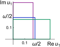
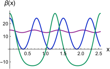
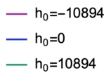
Note, if $\mathrm{b}$ is positive, than $\beta$ has maxima $-\mathrm{b}e_{1}$ at $x=n\omega/\mathrm{b}$, $n\in\operatorname{\mathbb{Z}}$, and minima $-\mathrm{b}e_{2}$ at $x=(n+\frac{1}{2})\omega/\mathrm{b}$, $n\in\operatorname{\mathbb{Z}}$. It follows from the fact that $\wp(\tfrac{1}{2}\omega^{\prime})=e_{1}$, $\wp(\tfrac{1}{2}\omega+\tfrac{1}{2}\omega^{\prime})=e_{2}$.

In terms of the Jacobi elliptic functions, we obtain the cnoidal wave, introduced by Korteweg and de Vries in [16]:

$$-\tfrac{1}{2}\wp(-\tfrac{1}{2}x+\tfrac{1}{2}\omega^{\prime}) +\tfrac{1}{6}(e_{1}+e_{2}+e_{3})$$

$$=-\tfrac{1}{2}\bigg{(}e_{2}+(e_{3}-e_{1})\frac{\operatorname{dn}\big{(}\imath K^{\prime}\mp\tfrac{1}{2}x\sqrt{e_{3}-e_{1}};k\big{)}^{2}}{\operatorname{sn}\big{(}\imath K^{\prime}\mp\tfrac{1}{2}x\sqrt{e_{3}-e_{1}};k\big{)}^{2}}\bigg{)}$$

$$=-\tfrac{1}{2}\Big{(}e_{2}-(e_{2}-e_{1})\operatorname{cn}\big{(}\tfrac{1}{2}x\sqrt{e_{3}-e_{1}};k\big{)}^{2}\Big{)},$$

where $k^{2}=(e_{2}-e_{1})/(e_{3}-e_{1})$, and $c_{2}\mathrm{b}^{-2}=-(e_{1}+e_{2}+e_{3})$.

7.3. Genus 2

The hamiltonian system of the KdV equation in $\mathcal{M}_{2}^{\circ}$ possesses the spectral curve

(58) $$-y^{2}+\mathrm{b}^{2}z^{5}+c_{3}z^{3}+c_{2}z^{2}+h_{1}z+h_{0}=0.$$

Requiring real-valued solutions, we suppose that all parameters $\mathrm{b}$, $c_{3}$, $c_{2}$, $h_{1}$, $h_{0}$ are real, and the spectral curve has five real branch points $e_{1}<e_{2}<e_{3}<e_{4}<e_{5}$. According to (37), uniformization of (58) is given by

(59) $$z^{2}=z\wp_{1,1}(u)+\wp_{1,3}(u),\qquad y=-\tfrac{1}{2}\mathrm{b}\big{(}z\wp_{1,1,1}(u)+\wp_{1,1,3}(u)\big{)},$$

where $u=(u_{1},u_{3})$, and the both components are complex, in general.

Bounded real-valued solutions in the case of $N=2$ are

(60) $$\beta(x)=-\mathrm{b}\wp_{1,1}(-\mathrm{b}x+C_{1},-\mathrm{b}t+C_{3}),$$

and by the reality conditions

$$\begin{split}&C_{1}=\tfrac{1}{2}\omega^{\prime}_{1,1}+\tfrac{1}{2}\omega^{\prime}_{1,2},\qquad C_{3}=\tfrac{1}{2}\omega^{\prime}_{3,1}+\tfrac{1}{2}\omega^{\prime}_{3,2},\end{split}$$

where $(\omega^{\prime}_{1,k},\omega^{\prime}_{3,k})^{t}=\omega^{\prime}_{k}$. First indices of the entries $\omega^{\prime}_{2i-1,k}$ correspond to the labels of holomorphic differentials $\mathrm{d}u_{2i-1}$, $i=1$, $2$, and $\omega^{\prime}_{1}$, $\omega^{\prime}_{2}$ are two columns of the period matrix $\omega^{\prime}$. On the subspace $-(\mathrm{b}x,\mathrm{b}t)^{t}+\tfrac{1}{2}\omega^{\prime}_{1}+\tfrac{1}{2}\omega^{\prime}_{2}$ the function $\wp_{1,1}$ is real-valued and bounded, with the critical values:

(61) $$\begin{split}&\wp_{1,1}(\tfrac{1}{2}\omega^{\prime}_{1}+\tfrac{1}{2}\omega^{\prime}_{2})=e_{2}+e_{3},\\ &\wp_{1,1}(\tfrac{1}{2}\omega_{1}+\tfrac{1}{2}\omega^{\prime}_{1}+\tfrac{1}{2}\omega^{\prime}_{2})=e_{1}+e_{3},\\ &\wp_{1,1}(\tfrac{1}{2}\omega_{2}+\tfrac{1}{2}\omega^{\prime}_{1}+\tfrac{1}{2}\omega^{\prime}_{2})=e_{2}+e_{4},\\ &\wp_{1,1}(\tfrac{1}{2}\omega_{1}+\tfrac{1}{2}\omega_{2}+\tfrac{1}{2}\omega^{\prime}_{1}+\tfrac{1}{2}\omega^{\prime}_{2})=e_{1}+e_{4}.\end{split}$$

Let $\mathcal{M}_{2}^{\circ}$ be fixed by $4\mathrm{b}^{2}=1$, $c_{4}=0$, $c_{3}=-15$, $c_{2}=-20$. Let the hamiltonians $h_{1}$, $h_{0}$ attains five values with different mutual positions of branch points: $h_{1}=-3$, $h_{0}=1$ $e_{1}\approx-6.99$, $e_{2}\approx-1.13$, $e_{3}\approx-0.39$ $e_{4}\approx 0.15$, $e_{5}\approx 8.35$;
$h_{1}=100$, $h_{0}=-56$ $e_{1}\approx-5.69$, $e_{2}\approx-4.55$, $e_{3}\approx 0.72$ $e_{4}\approx 1.50$, $e_{5}\approx 8.01$;
$h_{1}=100$, $h_{0}=81$ $e_{1}\approx-6.15$, $e_{2}\approx-3.52$, $e_{3}\approx-0.76$ $e_{4}\approx 2.48$, $e_{5}\approx 7.94$; $h_{1}=100$, $h_{0}=156$ $e_{1}\approx-6.30$, $e_{2}\approx-2.71$, $e_{3}\approx-1.67$ $e_{4}\approx 2.78$, $e_{5}\approx 7.90$; $h_{1}=210$, $h_{0}=460$ $e_{1}\approx-5.05$, $e_{2}\approx-3.86$, $e_{3}\approx-2.83$ $e_{4}\approx 4.76$, $e_{5}\approx 6.99$.

The corresponding fundamental domains are shown in two projections: on $u_{1}$, and $u_{3}$, see fig. 3. One can see a parallelogram spanned by $\frac{1}{2}\omega_{2i-1,1}$, $\frac{1}{2}\omega^{\prime}_{2i-1,1}$ drawn with a dashed line, a parallelogram spanned by $\frac{1}{2}\omega_{2i-1,2}$, $\frac{1}{2}\omega^{\prime}_{2i-1,2}$ drawn with a dotted line, and a parallelogram spanned by $\frac{1}{2}(\omega_{2i-1,1}+\omega_{2i-1,2})$, $\frac{1}{2}(\omega^{\prime}_{2i-1,1}+\omega^{\prime}_{2i-1,2})$ drawn with a solid line.

Figure 3. $N=2$. Fundamental domains.

3a. Projection on $u_{1}$                             3b. Projection on $u_{3}$    
            

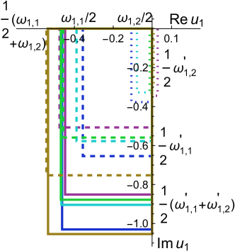
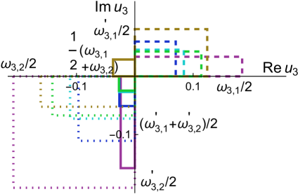
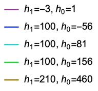
The corresponding shapes of $\beta$, according to (60) with $\mathrm{b}=1/2$, are presented on fig. 4 and 5. On fig. 4 the reader finds shapes of $\beta(x,0)$, $x\in[0,-20(\omega_{1,1}+\omega_{1,2})]$ (left column), and $\beta(0,t)$, $t\in[0,20]$ (right column). On fig. 5 shapes of $\beta(x,t)$, $x\in[0,-8(\omega_{1,1}+\omega_{1,2})]$, $t\in[0,-4\omega_{3,2}]$ are presented for the chosen values of $h_{1}$ and $h_{0}$. Dots on fig. 5 indicate critical values (61).

Figure 4. $N=2$. Quasi-periodic waves $\beta(x,0)$ (left) and $\beta(0,t)$ (right).

The cases $h_{1}=-3$, $h_{1}=100$, $h_{1}=210$, from the top to the bottom.
   
   
   

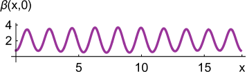
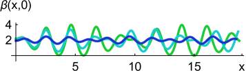
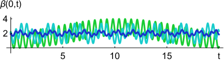
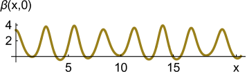
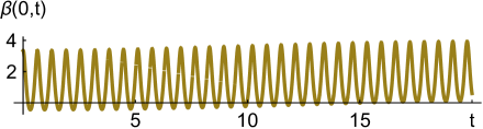
Figure 5. $N=2$. Quasi-periodic waves $\beta(x,t)$.

5a. $h_{1}=-3$, $h_{0}=1$.                             5b. $h_{1}=100$, $h_{0}=-56$.

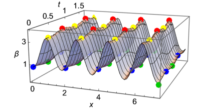
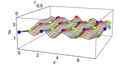
5c. $h_{1}=100$, $h_{0}=81$.                             5d. $h_{1}=100$, $h_{0}=156$.

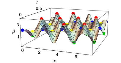
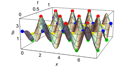
5e. $h_{1}=210$, $h_{0}=469$.                                                         
         

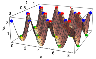
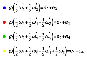
7.4. Genus $3$

The hamiltonian system of the KdV equation in $\mathcal{M}_{3}^{\circ}$ possesses the spectral curve

(62) $$-y^{2}+\mathrm{b}^{2}z^{7}+c_{5}z^{5}+c_{4}z^{4}+c_{3}z^{3}+h_{2}z^{2}+h_{1}z+h_{0}=0,$$

with all real parameters, chosen in such a way that all seven branch points are real. According to (37), uniformization of (62) is given by

(63) $$\begin{split}&z^{3}=z^{2}\wp_{1,1}(u)+z\wp_{1,3}(u)+\wp_{1,5}(u),\\ &y=-\tfrac{1}{2}\mathrm{b}\big{(}z^{2}\wp_{1,1,1}(u)+z\wp_{1,1,3}(u)+\wp_{1,1,5}(u)\big{)},\end{split}$$

where $u=(u_{1},u_{3},u_{5})$, and all components are complex, in general.

Bounded real-valued solutions in the case of $N=3$ are

(64) $$\beta(x)=-\mathrm{b}\wp_{1,1}(-\mathrm{b}x+C_{1},-\mathrm{b}t+C_{3},C_{5}),$$

and by the reality conditions,

$$\begin{split}&\qquad C_{1}=\tfrac{1}{2}\omega^{\prime}_{1,1}+\tfrac{1}{2}\omega^{\prime}_{1,2}+\tfrac{1}{2}\omega^{\prime}_{1,3},\\ &\qquad C_{3}=\tfrac{1}{2}\omega^{\prime}_{3,1}+\tfrac{1}{2}\omega^{\prime}_{3,2}+\tfrac{1}{2}\omega^{\prime}_{3,3},\\ &\qquad C_{5}=-\mathrm{c}+\tfrac{1}{2}\omega^{\prime}_{5,1}+\tfrac{1}{2}\omega^{\prime}_{5,2}+\tfrac{1}{2}\omega^{\prime}_{5,3},\quad\mathrm{c}\in\operatorname{\mathbb{R}},\end{split}$$

where $(\omega^{\prime}_{1,k},\omega^{\prime}_{3,k},\omega^{\prime}_{5,k})^{t}=\omega^{\prime}_{k}$. Recall that $\omega^{\prime}_{1}$, $\omega^{\prime}_{2}$, $\omega^{\prime}_{3}$ are three columns of the period matrix $\omega^{\prime}$. On $\tfrac{1}{2}\omega^{\prime}_{1}+\tfrac{1}{2}\omega^{\prime}_{2}+\tfrac{1}{2}\omega^{\prime}_{3}+\operatorname{\mathrm{Re}}\bar{\operatorname{\mathfrak{J}}}$ the function $\wp_{1,1}$ is real-valued and bounded, with the critical values:

(65) $$\begin{split}&\wp_{1,1}(\tfrac{1}{2}\omega^{\prime}_{1}+\tfrac{1}{2}\omega^{\prime}_{2}+\tfrac{1}{2}\omega^{\prime}_{3})=e_{1}+e_{4}+e_{5},\\ &\wp_{1,1}(\tfrac{1}{2}\omega_{1}+\tfrac{1}{2}\omega^{\prime}_{1}+\tfrac{1}{2}\omega^{\prime}_{2}+\tfrac{1}{2}\omega^{\prime}_{3})=e_{2}+e_{4}+e_{5},\\ &\wp_{1,1}(\tfrac{1}{2}\omega_{2}+\tfrac{1}{2}\omega^{\prime}_{1}+\tfrac{1}{2}\omega^{\prime}_{2}+\tfrac{1}{2}\omega^{\prime}_{3})=e_{1}+e_{3}+e_{5},\\ &\wp_{1,1}(\tfrac{1}{2}\omega_{1}+\tfrac{1}{2}\omega_{2}+\tfrac{1}{2}\omega^{\prime}_{1}+\tfrac{1}{2}\omega^{\prime}_{2}+\tfrac{1}{2}\omega^{\prime}_{3})=e_{2}+e_{3}+e_{5},\\ &\wp_{1,1}(\tfrac{1}{2}\omega_{3}+\tfrac{1}{2}\omega^{\prime}_{1}+\tfrac{1}{2}\omega^{\prime}_{2}+\tfrac{1}{2}\omega^{\prime}_{3})=e_{1}+e_{4}+e_{6},\\ &\wp_{1,1}(\tfrac{1}{2}\omega_{1}+\tfrac{1}{2}\omega_{3}+\tfrac{1}{2}\omega^{\prime}_{1}+\tfrac{1}{2}\omega^{\prime}_{2}+\tfrac{1}{2}\omega^{\prime}_{3})=e_{2}+e_{4}+e_{6},\\ &\wp_{1,1}(\tfrac{1}{2}\omega_{2}+\tfrac{1}{2}\omega_{3}+\tfrac{1}{2}\omega^{\prime}_{1}+\tfrac{1}{2}\omega^{\prime}_{2}+\tfrac{1}{2}\omega^{\prime}_{3})=e_{1}+e_{3}+e_{6},\\ &\wp_{1,1}(\tfrac{1}{2}\omega_{1}+\tfrac{1}{2}\omega_{2}+\tfrac{1}{2}\omega_{3}+\tfrac{1}{2}\omega^{\prime}_{1}+\tfrac{1}{2}\omega^{\prime}_{2}+\tfrac{1}{2}\omega^{\prime}_{3})=e_{2}+e_{3}+e_{6}.\end{split}$$

However, projection to the subspace $-(\mathrm{b}x,\mathrm{b}t,\mathrm{c})^{t}+\tfrac{1}{2}\omega^{\prime}_{1}+\tfrac{1}{2}\omega^{\prime}_{2}+\tfrac{1}{2}\omega^{\prime}_{3}$, which serves as the domain of the quasi-periodic KdV solution $\beta$, could contain not more than one of the values (65), if $\mathrm{c}$ is one of half-periods constructed from $\tfrac{1}{2}\omega_{1}$, $\tfrac{1}{2}\omega_{2}$, $\tfrac{1}{2}\omega_{3}$.

Let $\mathcal{M}_{3}^{\circ}$ be fixed by $4\mathrm{b}^{2}=1$, $c_{6}=0$, $c_{5}=-84$, $c_{4}=-160$, $c_{3}=7250$. Let the hamiltonians $h_{2}$, $h_{1}$, $h_{0}$ attain six values with different mutual positions of branch points. Computed by (64) with $\mathrm{b}=1/2$ and $\mathrm{c}=0$, shapes of $\beta(x,0)$, $x\in[0,-20(\omega_{1,1}+\omega_{1,3})]$, and $\beta(0,t)$, $t\in[0,10]$ or $t\in[0,20]$, are presented below.
$\vphantom{\displaystyle A^{\dfrac{A}{A}}}h_{2}=8178$, $h_{1}=-202052$, $h_{0}=111126;\qquad$ $e_{1}\approx-10.41$, $e_{2}\approx-10.30$, $e_{3}\approx-9.77$ $e_{4}\approx 0.57$, $e_{5}\approx 6.70$, $e_{6}\approx 6.75$, $e_{7}\approx 16.47$;    
$h_{2}=16678$, $h_{1}=-148832$, $h_{0}=-338529;\qquad$ $e_{1}\approx-11.44$, $e_{2}\approx-11.42$, $e_{3}\approx-5.67$ $e_{4}\approx-2.26$, $e_{5}\approx 5.41$, $e_{6}\approx 9.33$, $e_{7}\approx 16.04$;    
$h_{2}=12678$, $h_{1}=-172935$, $h_{0}=-12782;\qquad$ $e_{1}\approx-11.95$, $e_{2}\approx-9.07$, $e_{3}\approx-8.97$ $e_{4}\approx-0.07$, $e_{5}\approx 4.98$, $e_{6}\approx 8.84$, $e_{7}\approx 16.23$;    
$h_{2}=21460$, $h_{1}=-120322$, $h_{0}=-287405;\qquad$ $e_{1}\approx-12.88$, $e_{2}\approx-9.31$, $e_{3}\approx-6.21$ $e_{4}\approx-2.16$, $e_{5}\approx 4.31$, $e_{6}\approx 10.58$, $e_{7}\approx 15.67$;    
$h_{2}=22460$, $h_{1}=-81268$, $h_{0}=-267380\qquad$ $e_{1}\approx-12.21$, $e_{2}\approx-10.94$, $e_{3}\approx-3.57$ $e_{4}\approx-3.56$, $e_{5}\approx 3.62$, $e_{6}\approx 11.23$, $e_{7}\approx 15.44$;    
$h_{2}=32678$, $h_{1}=-63757$, $h_{0}=-372539\qquad$ $e_{1}\approx-13.85$, $e_{2}\approx-6.64$, $e_{3}\approx-5.10$ $e_{4}\approx-5.08$, $e_{5}\approx 3.35$, $e_{6}\approx 13.60$, $e_{7}\approx 13.72$.    

On fig. 6 shapes of $\beta(x,t)$, $x\in[0,6]$, $t\in[0,0.6]$ at some chosen values of $h_{2}$, $h_{1}$, $h_{0}$ are presented.

Figure 6. $N=3$. Quasi-periodic waves $\beta(x,t)$, $x\in[0,6]$, $t\in[0,0.6]$.

6a. $h_{2}=8178\vphantom{\displaystyle a^{\dfrac{a}{a}}}$,

$\phantom{mm}h_{1}=-202052$, $h_{0}=111126$.

6b. $h_{2}=16678\vphantom{\displaystyle a^{\dfrac{a}{a}}}$,

$\phantom{mm}h_{1}=-148832$, $h_{0}=-338529$.

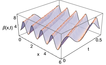
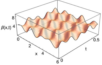
6c. $h_{2}=12678$,

$\phantom{mm}h_{1}=-172935$, $h_{0}=-12782$.

6c. $h_{2}=21460$,

$\phantom{mm}h_{1}=-120322$, $h_{0}=-287405$.

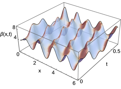
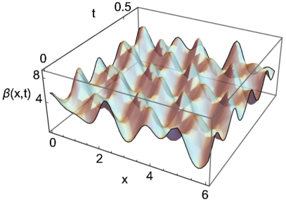
6e. $h_{2}=22460$,

$\phantom{mm}h_{1}=-81268$, $h_{0}=-267380$.

6f. $h_{2}=32678$,

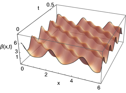
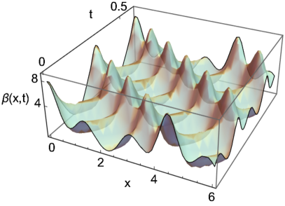
$\phantom{mm}h_{1}=-63757$, $h_{0}=-372539$.

References

- [1] Adler, M. On a trace functional for formal pseudo-differential operators and the symplectic structure of the Korteweg-devries type equations. Invent. Math. 50, 219–248 (1978).
- [2] Adler, M., Moerbeke P. Completely integrable systems, Euclidean Lie algebras, and curves. Advances in Math., 38:3, 267–317 (1980)
- [3] Baker H.F., Abelian functions: Abel’s theorem and the allied theory of theta functions, Cambridge, University press, Cambridge, 1897.
- [4] Baker H. F. An introduction to the theory of multiply periodic functions, Cambridge, University press, 1907.
- [5] Belokolos E. D., Bobenko A. I., Enolski V. Z., Its A. R., Matveev. V.B., Algebro-geometric approach to nonlinear integrable equations., Springer-Verhag, 1994
- [6] Bernatska J, Holod P. On Separation of variables for Integrable equations of soliton type, J. Nonlin. Math. Phys. 14:3 (2007) 353–374
- [7] Buchstaber V. M., Enolskii V. Z., and Leykin D. V., Hyperelliptic Kleinian functions and applications, preprint ESI 380 (1996), Vienna
- [8] Buchstaber V. M., Enolskii V. Z., Leykin D. V., Multi-dimensional sigma functions, arXiv:1208.0990
- [9] V. M. Buchstaber, D. V. Leikin, Addition laws on Jacobian varieties of plane algebraic curves, Nonlinear dynamics, Collected papers, Tr. Mat. Inst. Steklova, 251 (2005), pp. 54126.
- [10] Buchstaber V. M., and Leykin D. V. Solution of the problem of differentiation of abelian functions over parameters for families of -curves, Functional Analysis and Its Applications, 42:4, pp. 268–278, 2008
- [11] Faddeev L. D., Zakharov V. E., The Kortweg—deVries equation — a completely integrable Hamiltonian system, Functional Analysis and Its Applications, 5:4 (1971) 18–27.
- [12] Fomenko A. T., On symplectic structures and integrable systems on symmetric spaces, Math. USSR Sb. 43 (1982) 235
- [13] Gardner C., Green J., Kruskal M., and Miura R., A method for solving the Korteweg—de Vries equation, Phys. Rev. Lett., 19 (1967) 1095-1098.
- [14] Holod P., Integrable Hamiltonian systems of the orbits of affine Lie groups and periodic problem for modified Korteweg—de Vries equations, preprint ITP-82-144R, 1982 (in Russian).
- [15] Kadomtsev B. B., Karpman V. I., Nonlinear waves, Soviet Physics Uspekhi, 14:1 (1971) 40–60
- [16] Korteweg D. J., De Vries, G., On the change of form of long waves advancing in a rectangular canal, and on a new type of long stationary waves, Philosophical Magazine, 39:240 (1895) 422–443
- [17] Kostant B., The solution of a generalized Toda lattice and representation theory, Advances in Math., 34 (1979) 196–338
- [18] Kozel V. A. and Kotlyarov V. P. Explicit almost periodic solutions of the sine-Gordon equation Dokl. Akad. Nauk Ukr. SSR, Ser. A, 10 (1976) 878–881 (in Russian); translation in English in arXiv:1401.4410
- [19] P. Lax, Integrals of nonlinear equations of evolution and solitary waves, Comm. Pure Appl. Math., 21:2 (1968) 467–490.
- [20] Mishchenko A. S., Fomenko A. T., Euler equations on finite-dimensional Lie groups, Mathematics of the USSR: Izvestiya, textbf12:2 (1978) 371–389
- [21] Miura R. M., Gardner C. S., and Kruskal M., Kortweg-de Vries equation and generalizations, J. Math. Phys., 9:8 (1968) 1202–1209.
- [22] Novikov S. P., The periodic problem for the Korteweg—de Vries equation, Functional Analysis and Its Applications, 8:3 (1974) 236–246