The interior penalty virtual element method for fourth-order singular perturbation problems

Abstract

This paper is dedicated to the numerical solution of a fourth-order singular perturbation problem using the interior penalty virtual element method (IPVEM) proposed in [42]. The study introduces modifications to the jumps and averages in the penalty term, as well as presents an automated mesh-dependent selection of the penalty parameter. Drawing inspiration from the modified Morley finite element methods, we leverage the conforming interpolation technique to handle the lower part of the bilinear form. Through our analysis, we establish optimal convergence in the energy norm and provide a rigorous proof of uniform convergence concerning the perturbation parameter in the lowest-order case.

1 Introduction

Let $\Omega$ be a bounded polygonal domain of $\mathbb{R}^{2}$ with boundary $\partial\Omega$. For $f\in L^{2}(\Omega)$, we consider the following boundary value problem of the fourth-order singular perturbation equation:

$$\left\{\begin{array}[]{ll}\varepsilon^{2}\Delta^{2}u-\Delta u=f&{\rm in}~{}~{}\Omega,\\ u=\dfrac{\partial u}{\partial\bm{n}}=0&{\rm on}~{}~{}\partial\Omega,\end{array}\right.$$ (1.1)

where $\bm{n}=(n_{1},n_{2})$ is the unit outer normal to $\partial\Omega$, $\Delta$ is the standard Laplacian operator and $\varepsilon$ is a real parameter satisfying $0<\varepsilon\leq 1$. When $\varepsilon$ is not small, the problem can be numerically resolved as the biharmonic equation by using some standard finite element methods for fourth-order problems. However, in this article, we are primarily concerned with the case where $\varepsilon\to 0$, or the differential equation formally degenerates to the Poisson equation. Due to the presence of the fourth-order term, $H^{2}$-conforming finite elements with $C^{1}$ continuity were considered in [33], but these methods are quite complicated even in two dimensions. To overcome this difficulty, it is prefer to using nonconforming finite elements. Since the differential equation reduces to the Poisson equation in the singular limit, $C^{0}$-nonconforming finite elements are better suited for the task, as shown in [30]. In that work, the method was proved to converge uniformly in the perturbation parameter in the energy norm, and a counterexample was given to show that the Morley method diverges for the reduced second-order equation (see also the patch test in [38]). Considering that the Morley element has the least number of element degree of freedom (DoF), Wang et al. proposed in [39] a modified Morley element method. This method still uses the DoFs of the Morley element, but linear approximation of finite element functions is used in the lower part of the bilinear form:

$$\varepsilon^{2}a_{h}(u_{h},v_{h})+b_{h}(\Pi_{h}^{1}u_{h},\Pi_{h}^{1}v_{h})=(f,\Pi_{h}^{1}v_{h}),$$ (1.2)

where

$$a_{h}(v_{h},w_{h})=\sum\limits_{K\in\mathcal{T}_{h}}(\nabla^{2}v_{h},\nabla^{2}w_{h})_{K},\qquad b_{h}(v_{h},w_{h})=\sum\limits_{K\in\mathcal{T}_{h}}(\nabla v_{h},\nabla w_{h})_{K},$$

and $\Pi_{h}^{1}$ is the interpolation operator corresponding to linear conforming element for second-order partial differential equations. It was also shown that the modified method converges uniformly in the perturbation parameter. On the other hand, among the parameter-robust methods, the $C^{0}$ interior penalty methods [14, 12] may be most attractive as they utilize the standard $C^{0}$ finite element spaces. These spaces are primarily designed for solving second-order problems and effectively reduce the computational cost to a certain extent.

This paper focuses on virtual element methods (VEMs), which are a generalization of the standard finite element method that allows for general polytopal meshes. First proposed and analyzed in [7], with other pioneering works found in [2, 8], VEMs have several advantages over standard finite element methods. For example, they are more convenient for handling partial differential equations on complex geometric domains or those associated with high-regularity admissible spaces. To date, a considerable number of conforming and nonconforming VEMs have been developed to address second-order elliptic equations [2, 7, 23, 18] as well as fourth-order elliptic equations [16, 22, 6, 44, 20]. The versatility and effectiveness of the VEM have made it a popular choice for tackling a wide range of scientific and engineering problems, including the Stokes problem [5, 17, 29], the Navier-Stokes equation [10, 26, 11], the MHD equations [3, 9], the sine-Gordon equation [1], the topology optimization problems [21, 41, 5] and the variational and hemivariational inequalities [25, 35, 24, 36, 28, 32, 40, 37]. For a comprehensive understanding of recent advancements in the VEM, we recommend referring to the book [4] and the associated references. Additionally, with regards to the fourth-order singular perturbation problems, a notable application of the $C^{0}$-continuous nonconforming virtual element method can be found in [43].

Recently, the interior penalty technique for VEMs has been explored in [42] for the biharmonic equation, which is equipped with the same DoFs for the $H^{1}$-conforming virtual elements, and the new numerical scheme — the interior penalty virtual element method (IPVEM) — can be regarded as a combination of the virtual element space and discontinuous Galerkin scheme, since the resulting global discrete space is not $C^{0}$-continuous and an interior penalty formulation is adopted to enforce the $C^{1}$ continuity of the solution. Inspired by the technique in (1.2) for discontinuous elements, we are trying to explore the feasibility of the IPVEM for solving the fourth-order singular perturbation problem (1.1). In the context of VEMs, however, the linear conforming interpolation operator can be omitted as it yields the same elliptic projection.

The remainder of the paper is structured as follows. We begin by introducing the continuous variational problem and presenting some useful results in VEM analysis in Section 2. Section 3 is dedicated to the introduction of the IPVEM. In contrast to the jump and average terms in [42], we include the elliptic projector $\Pi_{h}^{\nabla}$ for all $v$ and $w$ in the penalty terms $J_{i}(v,w)$ for $i=1,2,3$ to simplify the implementation. Additionally, we provide an automated mesh-dependent selection of the penalty parameter $\lambda_{e}$, following a similar deduction as described in [31]. In Section 4, we establish the optimal convergence of the IPVEM in the energy norm and provide a uniform error estimate in the lowest-order case. Our analysis demonstrates that the IPVEM is robust with respect to the perturbation parameter. This is based on the observation that we can equivalently include the $H^{1}$-conforming interpolation in the lower part of the bilinear form, as in (1.2), since all required degrees of freedom are accessible. Numerical examples are presented in Section 5 to validate the theoretical predictions. Finally, conclusions are provided in the last section.

2 The continuous variational problem

We first introduce some notations and symbols frequently used in this paper. For a bounded Lipschitz domain $D$, the symbol $(\cdot,\cdot)_{D}$ denotes the $L^{2}$-inner product on $D$, $\|\cdot\|_{0,D}$ denotes the $L^{2}$-norm, and $|\cdot|_{s,D}$ is the $H^{s}(D)$-seminorm. For all integer $k\geq 0$, $\mathbb{P}_{k}(D)$ is the set of polynomials of degree $\leq k$ on $D$. Let $e\subset\partial K$ be the common edge for elements $K=K^{-}$ and $K^{+}$, and let $v$ be a scalar function defined on $e$. We introduce the jump and average of $v$ on $e$ by $[v]=v^{-}-v^{+}$ and $\{v\}=\frac{1}{2}(v^{-}+v^{+})$, where $v^{-}$ and $v^{+}$ are the traces of $v$ on $e$ from the interior and exterior of $K$, respectively. On a boundary edge, $[v]=v$ and $\{v\}=v$. Moreover, for any two quantities $a$ and $b$, “$a\lesssim b$” indicates “$a\leq Cb$” with the constant $C$ independent of the mesh size $h_{K}$, and “$a\eqsim b$” abbreviates “$a\lesssim b\lesssim a$”.

The variational formulation of (1.1) reads: Find $u\in V:=H_{0}^{2}(\Omega)$ such that

$$\varepsilon^{2}a(u,v)+b(u,v)=(f,v),\quad v\in H_{0}^{2}(\Omega),$$ (2.1)

where $a(u,v)=(\nabla^{2}u,\nabla^{2}v)$ and $b(u,v)=(\nabla u,\nabla v)$. To avoid complicated presentation, we confine our discussion in two dimensions, with the family of polygonal meshes $\{\mathcal{T}_{h}\}_{h>0}$ satisfying the following condition (cf. [15, 19]):

1. For each $K\in{\mathcal{T}}_{h}$, there exists a “virtual triangulation” ${\mathcal{T}}_{K}$ of $K$ such that ${\mathcal{T}}_{K}$ is uniformly shape regular and quasi-uniform. The corresponding mesh size of ${\mathcal{T}}_{K}$ is proportional to $h_{K}$. Each edge of $K$ is a side of a certain triangle in ${\mathcal{T}}_{K}$.

As shown in [19], this condition covers the usual geometric assumptions frequently used in the context of VEMs. Under this geometric assumption, we can establish some fundamental results in VEM analysis as used in [27].

According to the standard Dupont-Scott theory (cf. [13]), for all $v\in H^{l}(K)$ ($0\leq l\leq k$) there exists a certain $q\in\mathbb{P}_{l-1}(K)$ such that

$$|v-q|_{m,K}\lesssim h_{K}^{l-m}|v|_{l,K},\quad m\leq l.$$ (2.2)

The following trace inequalities are very useful for our forthcoming analysis.

Lemma 2.1.

For any $\varepsilon>0$, there exists a constant $C(\varepsilon)$ such that

$$\|v\|_{0,\partial K}^{2}\lesssim\|v\|_{0,K}\|v\|_{1,K},\quad v\in H^{1}(K),$$

$$\|v\|_{0,\partial K}\lesssim\varepsilon h_{K}^{1/2}|v|_{1,K}+C(\varepsilon)h_{K}^{-1/2}\|v\|_{0,K},\quad v\in H^{1}(K).$$

3 The interior penalty virtual element method

3.1 The $H^{1}$-projection in the lifting space

The interior penalty virtual element method (IPVEM) was proposed in [42]. In the construction, the authors first introduced a $C^{1}$-conforming virtual element space

$$\left\{v\in H^{2}(K):\Delta^{2}v\in\mathbb{P}_{k}(K),v|_{e}\in\mathbb{P}_{k+2}(e),\partial_{\bm{n}}v|_{e}\in\mathbb{P}_{k+1}(e),~{}~{}e\subset\partial K\right\},\quad k\geq 2,$$

which can be viewed as the lifting version of the standard $k$-th order $C^{1}$-conforming virtual element space for fourth-order singular perturbation problems. By checking the computability, we find that the order of the interior moments can be actually reduced to $k-2$. To this end, we instead consider the following modified lifting $C^{1}$-conforming virtual element space

$$\widetilde{V}_{k+2}(K)=\left\{v\in H^{2}(K):{\Delta^{2}v\in\mathbb{P}_{k-2}(K)},v|_{e}\in\mathbb{P}_{k+2}(e),\partial_{\bm{n}}v|_{e}\in\mathbb{P}_{k+1}(e),~{}~{}e\subset\partial K\right\}.$$

To present the degrees of freedom (DoFs), we introduce a scaled monomial $\mathbb{M}_{r}(D)$ on a $d$-dimensional domain $D$

$$\mathbb{M}_{r}(D):=\Big{\{}\Big{(}\frac{\bm{x}-\bm{x}_{D}}{h_{D}}\Big{)}^{\bm{s}},\quad|\bm{s}|\leq r\Big{\}},$$

where $h_{D}$ is the diameter of $D$, $\bm{x}_{D}$ the centroid of $D$, and $r$ a non-negative integer. For the multi-index ${\bm{s}}\in{\mathbb{N}^{d}}$, we follow the usual notation

$$\bm{x}^{\bm{s}}=x_{1}^{s_{1}}\cdots x_{d}^{s_{d}},\quad|\bm{s}|=s_{1}+\cdots+s_{d}.$$

Conventionally, $\mathbb{M}_{r}(D)=\{0\}$ for $r\leq-1$. This modified local space can be equipped with the following DoFs (cf. [16, 22]):

• $\tilde{\chi}^{v}:$ the values of $v$ at the vertices of $K$,

  $$\tilde{\chi}_{a}^{v}(v)=v(a),\quad\mbox{$a$ is a vertex of $K$}.$$

• $\tilde{\chi}^{g}$ : the values of $h_{a}\nabla v$ at the vertices of $K$,

  $$\tilde{\chi}_{a}^{g}(v)=h_{a}\nabla v(a),\quad\mbox{$a$ is a vertex of $K$},$$

  where $h_{a}$ is a characteristic length attached to each vertex $a$, for instance, the average of the diameters of the elements having $a$ as a vertex.

• $\tilde{\chi}^{e}$ : the moments of $v$ on edges up to degree $k-2$,

  $$\tilde{\chi}_{e}(v)=|e|^{-1}(m_{e},v)_{e},\quad m_{e}\in\mathbb{M}_{k-2}(e),\quad e\subset\partial K.$$

• $\tilde{\chi}^{n}$ : the moments of $\partial_{\bm{n}_{e}}v$ on edges up to degree $k-1$,

  $$\tilde{\chi}_{e}^{n}=(m_{e},\partial_{\bm{n}_{e}}v)_{e},\quad m_{e}\in\mathbb{M}_{k-1}(e),\quad e\subset\partial K.$$

• $\tilde{\chi}^{K}$ : the moments on element $K$ up to degree $k-2$,

  $$\tilde{\chi}_{K}(v)=|K|^{-1}(m_{K},v)_{K},\quad m_{K}\in\mathbb{M}_{k-2}(K).$$

Given $v_{h}\in\widetilde{V}_{k+2}(K)$, the usual definition of the $H^{1}$-elliptic projection $\Pi_{K}^{\nabla}v_{h}\in$ $\mathbb{P}_{k}(K)$ is described by the following equations:

$$\left\{\begin{aligned} (\nabla\Pi_{K}^{\nabla}v_{h},\nabla q)_{K}&=(\nabla v_{h},\nabla q)_{K},\quad q\in\mathbb{P}_{k}(K),\\ \sum\limits_{a\in\mathcal{V}_{K}}\Pi_{K}^{\nabla}v_{h}(a)&=\sum\limits_{a\in\mathcal{V}_{K}}v_{h}(a),\end{aligned}\right.$$ (3.1)

where $\mathcal{V}_{K}$ is the set of the vertices of $K$. This elliptic projection can be computed by the previous DoFs of $v_{h}$ by checking the right-hand side of the integration by parts formula:

$$(\nabla v_{h},\nabla q)_{K}=-(v_{h},\Delta q)_{K}+\sum\limits_{e\subset\partial K}\int_{e}v_{h}\partial_{\bm{n}_{e}}q\mathrm{d}s.$$

However, the goal of the IPVEM is to make $\Pi_{K}^{\nabla}v_{h}$ computable by only using the DoFs of $H^{1}$-conforming virtual element spaces given by (cf. [7, 2])

$$V_{h}^{1,c}(K):=\{v\in H^{1}(K):\Delta v|_{K}\in\mathbb{P}_{k-2}(K)~{}~{}{\text{in}}~{}~{}K,\quad v|_{\partial K}\in\mathbb{B}_{k}(\partial K)\},$$

where

$$\mathbb{B}_{k}(\partial K):=\{v\in C(\partial K):v|_{e}\in\mathbb{P}_{k}(e),\quad e\subset\partial K\}.$$

To do so, Ref. [42] considered the approximation of the RHS by some numerical formula. In view of the $\mathbb{P}_{k}$ accuracy, namely $\Pi_{K}^{\nabla}v_{h}=v_{h}$ for $v_{h}\in\mathbb{P}_{k}(K)$, the modified $H^{1}$-projection is defined as

$$\left\{\begin{aligned} (\nabla\Pi_{K}^{\nabla}v_{h},\nabla q)_{K}&=-(v_{h},\Delta q)_{K}+\sum\limits_{e\subset\partial K}Q_{2k-1}^{e}(v_{h}\partial_{\bm{n}_{e}}q),\quad q\in\mathbb{P}_{k}(K),\\ \sum_{a\in\mathcal{V}_{K}}\Pi_{K}^{\nabla}v_{h}(a)&=\sum_{a\in\mathcal{V}_{K}}v_{h}(a),\end{aligned}\right.$$

with

$$Q_{2k-1}^{e}v:=|e|\sum\limits_{i=0}^{k}\omega_{i}v(\bm{x}_{i}^{e})\approx\int_{e}v(s)\mathrm{d}s,$$

where $(\omega_{i},\bm{x}_{i}^{e})$ are the $(k+1)$ Gauss-Lobatto quadrature weights and points with $\bm{x}_{0}^{e}$ and $\bm{x}_{k}^{e}$ being the endpoints of $e$. The piecewise $H^{1}$-projector $\Pi_{h}^{\nabla}$ is defined by setting $\Pi_{h}^{\nabla}|_{K}=\Pi_{K}^{\nabla}$ for all $K\in\mathcal{T}_{h}$. In this case, the first and the third types of DoFs of $v_{h}$ on $e$ should be replaced by the $(k+1)$ Gauss-Lobatto points. Notice that when $v_{h}\in\mathbb{P}_{k}(K)$, the integrand of $\int_{e}v_{h}\partial_{\bm{n}_{e}}q\mathrm{d}s$ is a polynomial of order $2k-1$ on $e$, while the algebraic accuracy is exactly $2k-1$ for the $(k+1)$ Gauss-Lobatto points. In particular, we have $2k-1=3$ for $k=2$, corresponding to the Simpson’s rule.

Following the similar arguments in [42, Lemma 3.4] and [42, Corollary 3.7], we may derive the inverse inequalities and the boundedness of the $H^{1}$ projector described in the following Lemma.

Lemma 3.1.

For all $\,v_{h}\in\widetilde{V}_{k+2}(K)$ there hold

$$|v_{h}|_{m,K}\lesssim h_{K}^{s-m}|v_{h}|_{s,K},$$ (3.2)

$$|\Pi_{K}^{\nabla}v_{h}|_{m,K}\lesssim|v_{h}|_{m,K},$$ (3.3)

where $m=1,2$ and $0\leq s\leq m$.

3.2 The IP virtual element spaces

The $H^{1}$-elliptic projection is uniquely determined by the DoFs for the $H^{1}$-conforming virtual element space $V_{h}^{1,c}$. Because of this, one can replace the additional DoFs of $v\in\widetilde{V}_{k+2}(K)$ by the ones of $\Pi_{K}^{\nabla}v$. The local interior penalty space is then defined as

$$V_{k}(K)=\Big{\{}v\in\widetilde{V}_{k+2}(K):\tilde{\chi}^{g}(v)=\tilde{\chi}^{g}(\Pi_{K}^{\nabla}v),\tilde{\chi}^{n}(v)=\tilde{\chi}^{n}(\Pi_{K}^{\nabla}v)\Big{\}},$$

which satisfies $\Pi_{K}^{\nabla}v=v$ for $v\in\mathbb{P}_{k}(K)$, $\mathbb{P}_{k}(K)\subset V_{k}(K)$, and $V_{k}(K)\subset H^{2}(K)$. The associated DoFs are then given by

• $\chi^{v}:$ the values of $v(a)$, $a\in\mathcal{V}_{K}$;

• $\chi^{e}:$ the values of $v(\bm{x}_{i}^{e})$, $i=1,2\cdots,k-1$, $e\subset\partial K$;

• $\chi^{K}$ : the moments $|K|^{-1}(m_{K},v)_{K}$, $m_{K}\in\mathbb{M}_{k-2}(K)$.

Furthermore, we use $V_{h}$ to denote the global space of nonconforming virtual element, which is defined piecewise and required that the degrees of freedom are single-valued and vanish for the boundary DoFs.

Since $V_{h}$ and $V_{h}^{1,c}$ share the same DoFs, we can introduce the interpolation from $V_{h}$ to $V_{h}^{1,c}$. For any given $v_{h}\in V_{h}$, let $I_{h}^{c}v_{h}$ be the nodal interpolant of $v_{h}$ in $V_{h}^{1,c}$. One can define the $H^{1}$-elliptic projection $\Pi_{h}^{\nabla}I_{h}^{c}v_{h}$ as in (3.1) and find that

$$\Pi_{h}^{\nabla}I_{h}^{c}v_{h}=\Pi_{h}^{\nabla}v_{h},\quad v_{h}\in V_{h}$$ (3.4)

since $\bm{\chi}(I_{h}^{c}v_{h})=\bm{\chi}(v_{h})$ and $\Pi_{h}^{\nabla}$ is uniquely determined by the DoFs in $\bm{\chi}(v_{h})$. Here and below, $\bm{\chi}$ is the collection of the DoFs for $V_{h}$.

As usual, we can define the $H^{2}$-projection operator $\Pi_{K}^{\Delta}:V_{k}(K)\to\mathbb{P}_{k}(K)$ by finding the solution $\Pi_{K}^{\Delta}v\in\mathbb{P}_{k}(K)$ of

$$\begin{cases}a^{K}(\Pi_{K}^{\Delta}v,q)=a^{K}(v,q),\quad q\in\mathbb{P}_{k}(K),\\ \widehat{\Pi_{K}^{\Delta}v}=\widehat{v},\quad\widehat{\nabla\Pi_{K}^{\Delta}v}=\widehat{\nabla v}\end{cases}$$

for any given $v\in V_{k}(K)$, where the quasi-average $\widehat{v}$ is defined by

$$\widehat{v}=\frac{1}{|\partial K|}\int_{\partial K}v\mathrm{d}s.$$

3.3 The IP virtual element method with modified jump and penalty terms

Given the discrete bilinear form

$$a_{h}^{K}(v,w)=a^{K}(\Pi_{K}^{\Delta}v,\Pi_{K}^{\Delta}w)+S^{K}(v-\Pi_{K}^{\Delta}v,w-\Pi_{K}^{\Delta}w),\quad v,w\in V_{k}(K),$$

with

$$S^{K}(v-\Pi_{K}^{\Delta}v,w-\Pi_{K}^{\Delta}w)=h_{K}^{-2}\bm{\chi}(v-\Pi_{K}^{\Delta}v)\cdot\bm{\chi}(w-\Pi_{K}^{\Delta}w).$$

Let

$$J_{1}(v,w)=\sum_{e\in\mathcal{E}_{h}}\frac{\lambda_{e}}{|e|}\int_{e}\Big{[}\frac{\partial\Pi_{h}^{\nabla}v}{\partial\bm{n}_{e}}\Big{]}\Big{[}\frac{\partial\Pi_{h}^{\nabla}w}{\partial\bm{n}_{e}}\Big{]}\mathrm{d}s,$$

where $\lambda_{e}\geq 1$ is some edge-dependent parameter, and the additional terms are given by

$$J_{2}(v,w)=-\sum_{e\in\mathcal{E}_{h}}\int_{e}\Big{\{}\frac{\partial^{2}\Pi_{h}^{\nabla}v}{\partial\bm{n}_{e}^{2}}\Big{\}}\Big{[}\frac{\partial\Pi_{h}^{\nabla}w}{\partial\bm{n}_{e}}\Big{]}\mathrm{d}s,$$

$$J_{3}(v,w)=-\sum_{e\in\mathcal{E}_{h}}\int_{e}\Big{\{}\frac{\partial^{2}\Pi_{h}^{\nabla}w}{\partial\bm{n}_{e}^{2}}\Big{\}}\Big{[}\frac{\partial\Pi_{h}^{\nabla}v}{\partial\bm{n}_{e}}\Big{]}\mathrm{d}s.$$

In contrast to the jump and average terms in [42], here we include the elliptic projector $\Pi_{h}^{\nabla}$ for all $v$ and $w$ in $J_{i}$ for $i=1,2,3$ to simplify the implementation. According to the definition of $V_{k}(K)$, one easily finds that $J_{2}$ (or $J_{3}$) defined here coincides with the one given in [42], viz.,

$$J_{2}(v,w)=-\sum_{e\in\mathcal{E}_{h}}\int_{e}\Big{\{}\frac{\partial^{2}\Pi_{h}^{\nabla}v}{\partial\bm{n}_{e}^{2}}\Big{\}}\Big{[}\frac{\partial\Pi_{h}^{\nabla}w}{\partial\bm{n}_{e}}\Big{]}\mathrm{d}s=-\sum_{e\in\mathcal{E}_{h}}\int_{e}\Big{\{}\frac{\partial^{2}\Pi_{h}^{\nabla}v}{\partial\bm{n}_{e}^{2}}\Big{\}}\Big{[}\frac{\partial w}{\partial\bm{n}_{e}}\Big{]}\mathrm{d}s.$$

The IPVEM for the problem (1.1) can be described as follows: Find $u_{h}\in V_{h}$ such that

$$\varepsilon^{2}\mathcal{A}_{h}(u_{h},v_{h})+b_{h}(u_{h},v_{h})=\langle f_{h},v_{h}\rangle,\quad v_{h}\in V_{h},$$ (3.5)

where

$$\mathcal{A}_{h}(u_{h},v_{h})=a_{h}(u_{h},v_{h})+J_{1}(u_{h},v_{h})+J_{2}(u_{h},v_{h})+J_{3}(u_{h},v_{h}),$$ (3.6)

and $b_{h}(v,w)=\sum\limits_{K\in\mathcal{T}_{h}}b_{h}^{K}(v,w)$, with

$$b_{h}^{K}(v,w):=(\nabla\Pi_{K}^{\nabla}v,\nabla\Pi_{K}^{\nabla}w)+\bm{\chi}(v-\Pi_{K}^{\nabla}v)\cdot\bm{\chi}(w-\Pi_{K}^{\nabla}w).$$

The right-hand side is

$$\langle f_{h},v_{h}\rangle:=\sum\limits_{K\in\mathcal{T}_{h}}\int_{K}f\,\Pi_{0,K}^{k}v_{h}\mathrm{d}x,$$

with $\Pi_{0,K}^{k}$ being the $L^{2}$ projector onto $\mathbb{P}_{k}(K)$.

Remark 3.1.

In view of Eq. (3.4), we have

$$b_{h}^{K}(v,w)=b_{h}^{K}(v,I_{h}^{c}w),\quad v,w\in V_{h},$$ (3.7)

which is crucial in the error analysis. We also have

$$b_{h}^{K}(I_{h}^{c}v,I_{h}^{c}v)=b_{h}^{K}(v,I_{h}^{c}v),\quad v,w\in V_{h},$$ (3.8)

which implies

$$|I_{h}^{c}v_{h}|_{1,h}\lesssim|v_{h}|_{1,h}.$$ (3.9)

In what follows, we define

$$\|w\|_{h}^{2}:=|w|_{2,h}^{2}+J_{1}(w,w),\qquad\|w\|_{\varepsilon,h}^{2}:=\varepsilon^{2}\|w\|_{h}^{2}+|w|_{1,h}^{2}.$$ (3.10)

Lemma 3.2.

$\|\cdot\|_{h}$ and $\|\cdot\|_{\varepsilon,h}$ are norms on $V_{h}$.

Proof.

It is enough to prove that $\|v_{h}\|_{h}=0$ implies $v_{h}=0$ for any given $v_{h}\in V_{h}$. By definition, $\|v_{h}\|_{h}=0$ is equivalent to

$$|v_{h}|_{2,h}=0,\qquad J_{1}(v_{h},v_{h})=0.$$

The equation $|v_{h}|_{2,h}=0$ shows that $\nabla_{h}v_{h}$ is a piecewise constant on $\mathcal{T}_{h}$. On the other hand, the direct manipulation yields

$$\int_{e}\Big{[}\frac{\partial\Pi_{h}^{\nabla}v}{\partial\bm{n}_{e}}\Big{]}\Big{[}\frac{\partial\Pi_{h}^{\nabla}w}{\partial\bm{n}_{e}}\Big{]}\mathrm{d}s =:\int_{e}q_{k-1}^{e}\Big{[}\frac{\partial\Pi_{h}^{\nabla}w}{\partial\bm{n}_{e}}\Big{]}\mathrm{d}s=\int_{e}q_{k-1}^{e}\Big{[}\frac{\partial w}{\partial\bm{n}_{e}}\Big{]}\mathrm{d}s$$

$$=\int_{e}q_{k-1}^{e}\Pi^{k-1}_{0,e}\Big{[}\frac{\partial w}{\partial\bm{n}_{e}}\Big{]}\mathrm{d}s=\int_{e}\Big{[}\frac{\partial\Pi_{h}^{\nabla}v}{\partial\bm{n}_{e}}\Big{]}\Pi^{k-1}_{0,e}\Big{[}\frac{\partial w}{\partial\bm{n}_{e}}\Big{]}\mathrm{d}s$$

$$=\int_{e}\Big{[}\frac{\partial v}{\partial\bm{n}_{e}}\Big{]}\Pi^{k-1}_{0,e}\Big{[}\frac{\partial w}{\partial\bm{n}_{e}}\Big{]}\mathrm{d}s=\int_{e}\Pi^{k-1}_{0,e}\Big{[}\frac{\partial v}{\partial\bm{n}_{e}}\Big{]}\Pi^{k-1}_{0,e}\Big{[}\frac{\partial w}{\partial\bm{n}_{e}}\Big{]}\mathrm{d}s,$$ (3.11)

where $v,w\in V_{h}$. Thus, $J_{1}(v_{h},v_{h})=0$ implies $\Pi^{k-1}_{0,e}\Big{[}\frac{\partial v_{h}}{\partial\bm{n}_{e}}\Big{]}=0$, where $k\geq 2$. Since $\nabla_{h}v_{h}$ is piecewise constant, we further obtain $\Big{[}\frac{\partial v_{h}}{\partial\bm{n}_{e}}\Big{]}=0$ over the edges of $\mathcal{T}_{h}$. That is, the normal derivative of $v_{h}$ is continuous over interior edges and vanishes on the boundary of $\Omega$. This reduces to the discussion in the proof of Lemma 4.2 in [42], so we omit the remaining argument. ∎

3.4 Well-posedness of the discrete problem

In [42], the mesh-dependent parameter $\lambda_{e}$ was chosen as a sufficiently large constant $\lambda$. The stability for the bilinear forms can be obtained by using the similar arguments used in the proof of Theorem 4.3 in [42]. We omit the details with the results described as follows.

• $k$-consistency: for all $v\in V_{k}(K)$ and $q\in\mathbb{P}_{k}(K)$, it holds that

  $$a_{h}^{K}(v,q)=a^{K}(v,q),\quad b_{h}^{K}(v,q)=b^{K}(v,q).$$ (3.12)

• Stability: there exist two positive constants $\alpha_{*}$ and $\alpha^{*}$, independent of $h$, such that

  $$\alpha_{*}a^{K}(v,v)\leq a_{h}^{K}(v,v)\leq\alpha^{*}a^{K}(v,v),$$ (3.13)

  $$\alpha_{*}b^{K}(v,v)\leq b_{h}^{K}(v,v)\leq\alpha^{*}b^{K}(v,v)$$ (3.14)

  for all $v\in V_{k}(K)$.

Here, we aim to provide an automated mesh-dependent selection of $\lambda_{e}$ following a similar deduction with that described in [31].

Lemma 3.3.

For every constant $a$ satisfying

$$a>\max\Big{\{}1,\frac{1}{\sqrt{\alpha_{*}}}\Big{\}},$$

where $\alpha_{*}$ is given in (3.13), define the penalty parameter as

$$\lambda_{e}=\begin{cases}\dfrac{aN_{K}k(k-1)h_{e}^{2}}{4}\Big{(}\dfrac{1}{|T_{+}|}+\dfrac{1}{|T_{-}|}\Big{)},&\qquad e\in\mathcal{E}^{0},\\ \dfrac{aN_{K}k(k-1)h_{e}^{2}}{2|T_{+}|},&\qquad e\in\mathcal{E}^{\partial},\end{cases}$$

where $T_{+}$ and $T_{-}$ are the neighboring virtual triangles for an interior edge $e$, $T_{+}$ is the adjacent virtual triangle for a boundary edge $e$, and $N_{K}$ is the maximum number of edges of elements. Then there holds

$$\mathcal{A}_{h}(v_{h},v_{h})\geq\kappa\|v_{h}\|_{h}^{2}$$

with the constant

$$\kappa=\min\{\alpha_{*},1\}-\frac{1}{\sqrt{a}}.$$

Proof.

For every $\kappa>0$, consider the difference

$$\mathcal{A}_{h}(v_{h},v_{h})-\kappa\|v_{h}\|_{h}^{2} =(a_{h}(v_{h},v_{h})-\kappa|v_{h}|_{2,h}^{2})+(1-\kappa)J_{1}(v_{h},v_{h})+J_{2}(v_{h},v_{h})+J_{3}(v_{h},v_{h})$$

$$=(a_{h}(v_{h},v_{h})-\kappa|v_{h}|_{2,h}^{2})+(1-\kappa)J_{1}(v_{h},v_{h})+2J_{2}(v_{h},v_{h})$$

$$\geq(\alpha_{*}-\kappa)|v_{h}|_{2,h}^{2}+(1-\kappa)J_{1}(v_{h},v_{h})+2J_{2}(v_{h},v_{h}),$$

where the stability (3.13) is used. For every $\epsilon>0$, the Young’s inequality gives

$$2|J_{2}(v_{h},v_{h})| =2\Big{|}\sum_{e\in\mathcal{E}_{h}}\int_{e}\Big{\{}\frac{\partial^{2}\Pi_{h}^{\nabla}v_{h}}{\partial\bm{n}_{e}^{2}}\Big{\}}\Big{[}\frac{\partial\Pi_{h}^{\nabla}v_{h}}{\partial\bm{n}_{e}}\Big{]}\mathrm{d}s\Big{|}$$

$$\leq\sum_{e\in\mathcal{E}_{h}}\Big{(}\frac{\epsilon\lambda_{e}}{h_{e}}\Big{\|}\Big{[}\frac{\partial\Pi_{h}^{\nabla}v_{h}}{\partial\bm{n}_{e}}\Big{]}\Big{\|}_{0,e}^{2}+\frac{h_{e}}{\epsilon\lambda_{e}}\Big{\|}\Big{\{}\frac{\partial^{2}\Pi_{h}^{\nabla}v_{h}}{\partial\bm{n}_{e}^{2}}\Big{\}}\Big{\|}_{0,e}^{2}\Big{)}$$

$$=\epsilon J_{1}(v_{h},v_{h})+\sum_{e\in\mathcal{E}_{h}}\frac{h_{e}}{\epsilon\lambda_{e}}\Big{\|}\Big{\{}\frac{\partial^{2}\Pi_{h}^{\nabla}v_{h}}{\partial\bm{n}_{e}^{2}}\Big{\}}\Big{\|}_{0,e}^{2}.$$

This reduces to the estimate of the average $\Big{\{}\frac{\partial^{2}\Pi_{h}^{\nabla}v_{h}}{\partial\bm{n}_{e}^{2}}\Big{\}}=\Big{\{}\bm{n}_{e}^{T}(\nabla_{h}^{2}\Pi_{h}^{\nabla}v_{h})\bm{n}_{e}\Big{\}}$.

For an interior edge $e$ with the neighboring virtual triangles $T_{+}$ and $T_{-}$, the definition of the average and the Young’s inequality give

$$\Big{\|}\Big{\{}\frac{\partial^{2}\Pi_{h}^{\nabla}v_{h}}{\partial\bm{n}_{e}^{2}}\Big{\}}\Big{\|}_{0,e}^{2} =\Big{\|}\frac{1}{2}n_{e}^{T}((\nabla_{h}^{2}\Pi_{h}^{\nabla}v_{h})|_{T_{+}}+(\nabla_{h}^{2}\Pi_{h}^{\nabla}v_{h})|_{T_{-}})n_{e}\Big{\|}_{0,e}^{2}$$

$$\leq\frac{1}{4}\|(\nabla_{h}^{2}\Pi_{h}^{\nabla}v_{h})|_{T_{+}}+(\nabla_{h}^{2}\Pi_{h}^{\nabla}v_{h})|_{T_{-}}\|_{0,e}^{2}$$

$$=\frac{1}{4}(\|(\nabla_{h}^{2}\Pi_{h}^{\nabla}v_{h})|_{T_{+}}\|_{0,e}^{2}+\|(\nabla_{h}^{2}\Pi_{h}^{\nabla}v_{h})|_{T_{-}}\|_{0,e}^{2}+2\int_{e}(\nabla_{h}^{2}\Pi_{h}^{\nabla}v_{h})|_{T_{+}}(\nabla_{h}^{2}\Pi_{h}^{\nabla}v_{h})|_{T_{-}}\mathrm{d}s$$

$$\leq\frac{1}{4}\Big{(}(1+\alpha)\|(\nabla_{h}^{2}\Pi_{h}^{\nabla}v_{h})|_{T_{+}}\|_{0,e}^{2}+(1+\frac{1}{\alpha})\|(\nabla_{h}^{2}\Pi_{h}^{\nabla}v_{h})|_{T_{-}}\|_{0,e}^{2}\Big{)}$$ (3.15)

for any $\alpha>0$. Since $(\nabla_{h}^{2}\Pi_{h}^{\nabla}v_{h})|_{T_{\pm}}$ are polynomials of degree $k-2$, this and Lemma 3.4 in [31] result in

$$\Big{\|}\Big{\{}\frac{\partial^{2}\Pi_{h}^{\nabla}v_{h}}{\partial\bm{n}_{e}^{2}}\Big{\}}\Big{\|}_{0,e}^{2}\leq\frac{k(k-1)h_{e}}{8}\Big{(}\frac{1+\alpha}{|T_{+}|}\|\nabla_{h}^{2}\Pi_{h}^{\nabla}v_{h}\|_{0,T_{+}}^{2}+\frac{1+1/\alpha}{|T_{-}|}\|\nabla_{h}^{2}\Pi_{h}^{\nabla}v_{h}\|_{0,T_{-}}^{2}\Big{)}.$$

The optimal value $\alpha=|T_{+}|/|T_{-}|$ and the boundedss of $\Pi_{h}^{\nabla}$ in (3.3) of Lemma 3.1 lead to

$$\Big{\|}\Big{\{}\frac{\partial^{2}\Pi_{h}^{\nabla}v_{h}}{\partial\bm{n}_{e}^{2}}\Big{\}}\Big{\|}_{0,e}^{2} \leq\frac{k(k-1)h_{e}}{8}\Big{(}\frac{1}{|T_{+}|}+\frac{1}{|T_{-}|}\Big{)}\|\nabla_{h}^{2}\Pi_{h}^{\nabla}v_{h}\|_{0,T_{+}\cup T_{-}}$$

$$\leq\frac{k(k-1)h_{e}}{8}\Big{(}\frac{1}{|T_{+}|}+\frac{1}{|T_{-}|}\Big{)}|v_{h}|_{2,K_{+}\cup K_{-}}.$$ (3.16)

For a boundary edge $e$ with adjacent virtual triangle $T_{+}$, we can get

$$\Big{\|}\Big{\{}\frac{\partial^{2}\Pi_{h}^{\nabla}v_{h}}{\partial\bm{n}_{e}^{2}}\Big{\}}\Big{\|}_{0,e}^{2}\leq\frac{k(k-1)h_{e}}{2|T_{+}|}\|\nabla_{h}^{2}\Pi_{h}^{\nabla}v_{h}\|_{0,T_{+}}\leq\frac{k(k-1)h_{e}}{2|T_{+}|}|v_{h}|_{2,K_{+}}.$$

Consequently, with the choice of $\lambda_{e}$, the sum over all edges and the finite overlap of the edge patches lead to

$$2|J_{2}(v_{h},v_{h})|\leq\epsilon J_{1}(v_{h},v_{h})+\frac{1}{a\epsilon}|v_{h}|_{2,h}.$$

The above discussion gives

$$\mathcal{A}_{h}(v_{h},v_{h})-\kappa\|v_{h}\|_{h}^{2} \geq(\alpha_{*}-\frac{1}{a\epsilon}-\kappa)|v_{h}|_{2,h}^{2}+(1-\epsilon-\kappa)J_{1}(v_{h},v_{h}).$$

Every choice of $0<\kappa\leq\min\{\alpha_{*}-1/(a\epsilon),1-\epsilon\}$ leads to a nonnegative lower bound, and so proves the claim that

$$\mathcal{A}_{h}(v_{h},v_{h})\geq\kappa\|v_{h}\|_{h}^{2}.$$

Taking $\epsilon=1/\sqrt{a}$ with $a>\max\{1,\frac{1}{\sqrt{\alpha_{*}}}\}$ results in

$$\kappa:=\min\Big{\{}\alpha_{*}-\frac{1}{\sqrt{a}},1-\frac{1}{\sqrt{a}}\Big{\}}=\min\{\alpha_{*},1\}-\frac{1}{\sqrt{a}},$$

as required. ∎

Remark 3.2.

We remark that the lower and upper bounds of $\lambda_{e}$ are independent of mesh sizes, namely, $\lambda_{e}\eqsim 1$, under the given mesh assumption.

Theorem 3.1.

For the parameter $\lambda_{e}$ chosen as in Lemma 3.3, there exists a unique solution to the discrete problem (3.5).

Proof.

For any $v_{h}\in V_{h}$, Lemma 3.3 along with the stability (3.14) yields the coercivity

$$\varepsilon^{2}\mathcal{A}_{h}(v_{h},v_{h})+b_{h}(v_{h},v_{h})\geq\varepsilon^{2}\kappa\|v_{h}\|_{h}^{2}+\alpha_{*}|v_{h}|_{1,h}^{2}\geq\min\{\kappa,\alpha_{*}\}\|v_{h}\|_{\varepsilon,h}^{2}=\alpha_{*}\|v_{h}\|_{\varepsilon,h}^{2}$$ (3.17)

For the boundedness of the bilinear form, by the definition of $\interleave\cdot\interleave_{h}$ given in (3.10), it suffices to consider $\varepsilon^{2}J_{2}(v_{h},w_{h})$ for any $v_{h},w_{h}\in V_{h}$. The Cauchy-Schwarz inequality gives

$$|J_{2}(v_{h},w_{h})| =\Big{|}\sum_{e\in\mathcal{E}_{h}}\int_{e}\Big{\{}\frac{\partial^{2}\Pi_{h}^{\nabla}v_{h}}{\partial\bm{n}_{e}^{2}}\Big{\}}\Big{[}\frac{\partial\Pi_{h}^{\nabla}w_{h}}{\partial\bm{n}_{e}}\Big{]}\mathrm{d}s\Big{|}$$

$$\lesssim\Big{(}\sum_{e\in\mathcal{E}_{h}}\frac{h_{e}}{\lambda_{e}}\Big{\|}\Big{\{}\frac{\partial^{2}\Pi_{h}^{\nabla}v_{h}}{\partial\bm{n}_{e}^{2}}\Big{\}}\Big{\|}_{e}^{2}\Big{)}^{\frac{1}{2}}\Big{(}\sum_{e\in\mathcal{E}_{h}}\frac{\lambda_{e}}{h_{e}}\Big{\|}\Big{[}\frac{\partial\Pi_{h}^{\nabla}w_{h}}{\partial\bm{n}_{e}}\Big{]}\Big{\|}_{e}^{2}\Big{)}^{\frac{1}{2}}$$

$$=\Big{(}\sum_{e\in\mathcal{E}_{h}}\frac{h_{e}}{\lambda_{e}}\Big{\|}\Big{\{}\frac{\partial^{2}\Pi_{h}^{\nabla}v_{h}}{\partial\bm{n}_{e}^{2}}\Big{\}}\Big{\|}_{e}^{2}\Big{)}^{\frac{1}{2}}J_{1}(w_{h},w_{h})^{1/2}.$$ (3.18)

For an interior edge $e$ with the neighboring virtual triangles $T_{+}$ and $T_{-}$, we obtain from (3.16) and the definition of $\lambda_{e}$ that

$$\frac{h_{e}}{\lambda_{e}}\Big{\|}\Big{\{}\frac{\partial^{2}\Pi_{h}^{\nabla}v_{h}}{\partial\bm{n}_{e}^{2}}\Big{\}}\Big{\|}_{0,e}^{2}\leq\frac{k(k-1)h_{e}}{8}\Big{(}\frac{1}{|T_{+}|}+\frac{1}{|T_{-}|}\Big{)}|v_{h}|_{2,K_{+}\cup K_{-}}=\frac{1}{2aN_{K}}|v_{h}|_{2,K_{+}\cup K_{-}},$$

where $a$ and $N_{K}$ are defined in Lemma 3.3. For a boundary edge $e$, one can get

$$\frac{h_{e}}{\lambda_{e}}\Big{\|}\Big{\{}\frac{\partial^{2}\Pi_{h}^{\nabla}v_{h}}{\partial\bm{n}_{e}^{2}}\Big{\}}\Big{\|}_{0,e}^{2}\leq\frac{1}{aN_{K}}|v_{h}|_{2,K_{+}}.$$

Therefore,

$$\Big{(}\sum_{e\in\mathcal{E}_{h}}\frac{h_{e}}{\lambda_{e}}\Big{\|}\Big{\{}\frac{\partial^{2}\Pi_{h}^{\nabla}v_{h}}{\partial\bm{n}_{e}^{2}}\Big{\}}\Big{\|}_{e}^{2}\Big{)}^{\frac{1}{2}}\lesssim|v_{h}|_{2,h},$$

which together with (3.18) yields

$$|\varepsilon^{2}J_{2}(v_{h},w_{h})|\lesssim\|v_{h}\|_{\varepsilon,h}\|w_{h}\|_{\varepsilon,h}.$$

The proof is finished by using the Lax-Milgram lemma. ∎

4 Error analysis

4.1 An abstract Strang-type lemma

For any function $v\in H_{0}^{1}(\Omega)\cap H^{2}(\Omega)$, its interpolation $I_{h}v$ is defined by the condition that $v$ and $I_{h}v$ have the same degrees of freedom:

$$\chi_{i}(I_{h}v)=\chi_{i}(v),\qquad\chi_{i}\in\bm{\chi}.$$

Since the computation of the elliptic projection $\Pi_{h}^{\nabla}I_{h}u$ only involves the DoFs of $u$ and $\bm{\chi}(I_{h}u)=\bm{\chi}(u)$, we define $\Pi_{h}^{\nabla}u=\Pi_{h}^{\nabla}I_{h}u$ in what follows, which makes the expressions $\|u-u_{h}\|_{\varepsilon,h}$, $\|u-I_{h}u\|_{\varepsilon,h}$ and $\|u-u_{\pi}\|_{\varepsilon,h}$ well-defined in the following lemma, where $u$ is the exact solution to (1.1).

Lemma 4.1.

Assume that $u\in H_{0}^{2}(\Omega)\cap H^{3}(\Omega)$ is the exact solution to (1.1). Then we have the error estimate

$$\|u-u_{h}\|_{\varepsilon,h}\lesssim\|u-I_{h}u\|_{\varepsilon,h}+\|u-u_{\pi}\|_{\varepsilon,h}+\|f-f_{h}\|_{V_{h}^{\prime}}+E_{h},$$ (4.1)

where $u_{\pi}$ is a piecewise polynomial,

$$\|f-f_{h}\|_{V_{h}^{\prime}}=\sup_{v_{h}\in V_{h}\backslash\{0\}}\frac{\langle f-f_{h},v_{h}\rangle}{\|v_{h}\|_{\varepsilon,h}}$$

and the consistency term

$$E_{h}=\sup_{v_{h}\in V_{h}\backslash\{0\}}\frac{E_{A}(u,v_{h})+E_{J}(u,v_{h})}{\|v_{h}\|_{\varepsilon,h}},$$ (4.2)

with

$$E_{A}(u,v_{h})=\sum\limits_{K\in\mathcal{T}_{h}}(\varepsilon^{2}a^{K}(u,v_{h})+b^{K}(u,I_{h}^{c}v_{h}))-(f,v_{h}),$$

$$E_{J}(u,v_{h})=\varepsilon^{2}(J_{1}(I_{h}u,v_{h})+J_{2}(I_{h}u,v_{h})+J_{3}(I_{h}u,v_{h})),$$

where $I_{h}^{c}$ is the conforming interpolation operator defined in Section 3.2.

Proof.

Let $\delta_{h}:=I_{h}u-u_{h}$. We have by the coercivity (3.17) and the definition of the discrete problem (3.5) that

$$\alpha_{*}\|\delta_{h}\|_{\varepsilon,h}^{2} \leq\varepsilon^{2}\Big{(}a_{h}(\delta_{h},\delta_{h})+J_{1}(\delta_{h},\delta_{h})+J_{2}(\delta_{h},\delta_{h})+J_{3}(\delta_{h},\delta_{h})\Big{)}+b_{h}(\delta_{h},\delta_{h})$$

$$=\varepsilon^{2}\Big{(}a_{h}(I_{h}u,\delta_{h})+J_{1}(I_{h}u,\delta_{h})+J_{2}(I_{h}u,\delta_{h})+J_{3}(I_{h}u,\delta_{h})\Big{)}+b_{h}(I_{h}u,\delta_{h})-\langle f_{h},\delta_{h}\rangle$$

$$=\varepsilon^{2}a_{h}(I_{h}u,\delta_{h})+b_{h}(I_{h}u,I_{h}^{c}\delta_{h})-(f,\delta_{h})+\langle f-f_{h},\delta_{h}\rangle+E_{J}(u,v_{h}),$$

where we have used (3.7) in Remark 3.1.

According to the $k$-consistency (3.12) and the stability formulas (3.13) and (3.14), combing with (3.9), we get

$$\varepsilon^{2}a_{h}(I_{h}u,\delta_{h})+b_{h}(I_{h}u,\delta_{h})-(f,\delta_{h})$$

$$=\sum_{K\in\mathcal{T}_{h}}\varepsilon^{2}(a_{h}^{K}(I_{h}u-u_{\pi},\delta_{h})+a^{K}(u_{\pi}-u,\delta_{h}))+\sum_{K\in\mathcal{T}_{h}}(b_{h}^{K}(I_{h}u-u_{\pi},\delta_{h})+b^{K}(u_{\pi}-u,I_{h}^{c}\delta_{h}))$$

$$\qquad+\sum\limits_{K\in\mathcal{T}_{h}}(\varepsilon^{2}a^{K}(u,\delta_{h})+b^{K}(u,I_{h}^{c}\delta_{h}))-(f,\delta_{h})$$

$$\leq\varepsilon^{2}(|u-I_{h}u|_{2,h}+|u-u_{\pi}|_{2,h})|\delta_{h}|_{2,h}+(|u-I_{h}u|_{1,h}+|u-u_{\pi}|_{1,h})|\delta_{h}|_{1,h}+E_{A}(u,v_{h})$$

$$\lesssim(\|u-I_{h}u\|_{\varepsilon,h}+\|u-u_{\pi}\|_{\varepsilon,h})\|\delta_{h}\|_{\varepsilon,h}+E_{A}(u,v_{h}).$$

The proof is completed by using the triangle inequality. ∎

Lemma 4.2.

One can get rid of $\varepsilon^{2}J_{2}(I_{h}u,v_{h})$ in the consistency term (4.2) and obtain

$$E_{A}(u,v_{h})+E_{J}(u,v_{h})=E_{A1}+E_{A2}+E_{A3}+\varepsilon^{2}(J_{1}(I_{h}u,v_{h})+J_{3}(I_{h}u,v_{h})),$$

where

$$E_{A1}=\varepsilon^{2}\sum_{e\in\mathcal{E}_{h}}\int_{e}\Big{\{}\frac{\partial^{2}(u-\Pi_{h}^{\nabla}I_{h}u)}{\partial\bm{n}_{e}^{2}}\Big{\}}\left[\frac{\partial v_{h}}{\partial\bm{n}_{e}}\right]\mathrm{d}s,\qquad E_{A2}=\varepsilon^{2}\sum_{e\in\mathcal{E}_{h}}\int_{e}\frac{\partial^{2}u}{\partial\bm{n}_{e}\partial\bm{t}_{e}}\left[\frac{\partial v_{h}}{\partial\bm{t}_{e}}\right]\mathrm{d}s,$$

$$E_{A3}=-\varepsilon^{2}\sum_{K\in\mathcal{T}_{h}}(\nabla\Delta u,\nabla v_{h})_{K}+\sum_{K\in\mathcal{T}_{h}}(\nabla u,\nabla I_{h}^{c}v_{h})_{K}-(f,v_{h}).$$

Proof.

For brevity, we use the summation convention whereby summation is implied when an index is repeated exactly two times. For any given $v_{h}\in V_{h}$, the integration by parts gives

$$a^{K}(u,v_{h})=(\nabla^{2}u,\nabla^{2}v_{h})_{K}=\int_{K}\partial_{ij}u\partial_{ij}v_{h}\mathrm{d}x=\int_{\partial K}\partial_{ij}un_{j}\partial_{i}v_{h}\mathrm{d}s-\int_{K}\partial_{ijj}u\partial_{i}v_{h}\mathrm{d}x,$$

where $\bm{n}_{K}=(n_{1},n_{2})$. Since $\partial_{i}v=n_{i}\partial_{\bm{n}}v+t_{i}\partial_{\bm{t}}v$, we immediately obtain

$$a^{K}(u,v_{h}) =\int_{\partial K}\partial_{ij}un_{i}n_{j}\partial_{\bm{n}}v_{h}\mathrm{d}s+\int_{\partial K}\partial_{ij}ut_{i}n_{j}\partial_{\bm{t}}v_{h}\mathrm{d}s-\int_{K}\partial_{ijj}u\partial_{i}v_{h}\mathrm{d}x$$

$$=\int_{\partial K}\frac{\partial^{2}u}{\partial\bm{n}_{K}^{2}}\frac{\partial v_{h}}{\partial\bm{n}_{K}}\mathrm{d}s+\int_{\partial K}\frac{\partial^{2}u}{\partial\bm{n}_{K}\partial\bm{t}_{K}}\frac{\partial v_{h}}{\partial\bm{t}_{K}}\mathrm{d}s-(\nabla\Delta u,\nabla v_{h})_{K}.$$

Therefore,

$$E_{A}(u,v_{h}) :=\sum\limits_{K\in\mathcal{T}_{h}}(\varepsilon^{2}a^{K}(u,v_{h})+b^{K}(u,I_{h}^{c}v_{h}))-(f,v_{h})$$

$$=\varepsilon^{2}\sum_{e\in\mathcal{E}_{h}}\int_{e}\Big{(}\frac{\partial^{2}u}{\partial\bm{n}_{e}^{2}}\left[\frac{\partial v_{h}}{\partial\bm{n}_{e}}\right]+\frac{\partial^{2}u}{\partial\bm{n}_{e}\partial\bm{t}_{e}}\left[\frac{\partial v_{h}}{\partial\bm{t}_{e}}\right]\Big{)}\mathrm{d}s$$

$$\qquad-\varepsilon^{2}\sum_{K\in\mathcal{T}_{h}}(\nabla\Delta u,\nabla v_{h})_{K}+\sum_{K\in\mathcal{T}_{h}}(\nabla u,\nabla I_{h}^{c}v_{h})_{K}-(f,v_{h})$$

$$=:\widetilde{E}_{A1}+E_{A2}+E_{A3},$$ (4.3)

where

$$\widetilde{E}_{A1}=\varepsilon^{2}\sum_{e\in\mathcal{E}_{h}}\int_{e}\frac{\partial^{2}u}{\partial\bm{n}_{e}^{2}}\left[\frac{\partial v_{h}}{\partial\bm{n}_{e}}\right]\mathrm{d}s,$$

and $E_{A2}$ and $E_{A3}$ are defined as in the lemma. For $\widetilde{E}_{A1}$, we consider the decomposition

$$\widetilde{E}_{A1} =\varepsilon^{2}\sum_{e\in\mathcal{E}_{h}}\int_{e}\Big{\{}\frac{\partial^{2}(u-\Pi_{h}^{\nabla}I_{h}u)}{\partial\bm{n}_{e}^{2}}\Big{\}}\left[\frac{\partial v_{h}}{\partial\bm{n}_{e}}\right]\mathrm{d}s+\varepsilon^{2}\sum_{e\in\mathcal{E}_{h}}\int_{e}\Big{\{}\frac{\partial^{2}\Pi_{h}^{\nabla}I_{h}u}{\partial\bm{n}_{e}^{2}}\Big{\}}\left[\frac{\partial v_{h}}{\partial\bm{n}_{e}}\right]\mathrm{d}s$$

$$=\varepsilon^{2}\sum_{e\in\mathcal{E}_{h}}\int_{e}\Big{\{}\frac{\partial^{2}(u-\Pi_{h}^{\nabla}I_{h}u)}{\partial\bm{n}_{e}^{2}}\Big{\}}\left[\frac{\partial v_{h}}{\partial\bm{n}_{e}}\right]\mathrm{d}s-\varepsilon^{2}J_{2}(I_{h}u,v_{h})=E_{A1}-\varepsilon^{2}J_{2}(I_{h}u,v_{h}).$$

The result follows from Lemma 4.1. ∎

4.2 Error estimate

For $3\leq s\leq k+1$, the estimate of the load term is

$$\langle f-f_{h},v_{h}\rangle =\sum_{K\in\mathcal{T}_{h}}(f,v_{h}-\Pi_{0,K}^{k}v_{h})_{K}=\sum_{K\in\mathcal{T}_{h}}(f-\Pi_{0,K}^{k}f,v_{h}-\Pi_{0,K}^{k}v_{h})_{K}$$

$$\lesssim h^{s-3}\|f\|_{s-3}h|v_{h}|_{1,h}\lesssim h^{s-2}\|f\|_{s-3}\|v_{h}\|_{\varepsilon,h},$$

namely,

$$\|f-f_{h}\|_{V_{h}^{\prime}}\lesssim h^{s-2}\|f\|_{s-3}.$$ (4.4)

As shown in Lemma 3.11 of [42], we can derive the interpolation error estimate for our IPVEM.

Lemma 4.3.

For any $v\in H_{0}^{1}(\Omega)\cap H^{s}(\Omega)$ with $2\leq s\leq k+1$, it holds

$$|v-I_{h}v|_{m,K}\lesssim h_{K}^{s-m}|v|_{s,K},\quad m=0,1,2,\quad K\in\mathcal{T}_{h}.$$

We now consider the consistency term in Lemma 4.1.

Lemma 4.4.

Assume that $u\in H_{0}^{2}(\Omega)\cap H^{s}(\Omega)$ is the exact solution to (1.1) with $3\leq s\leq k+1$. Then the consistency error is bounded by

$$E_{h}\lesssim h^{s-2}(\varepsilon|u|_{s}+\|f\|_{s-3}).$$ (4.5)

Proof.

For clarity, we divide the proof into two steps.

Step 1: According to Lemma 4.2, one has

$$E_{A}(u,v_{h})+E_{J}(u,v_{h}) =E_{A1}+E_{A2}+E_{A3}+\varepsilon^{2}(J_{1}(I_{h}u,v_{h})+J_{3}(I_{h}u,v_{h}))$$

$$=\varepsilon^{2}\sum_{e\in\mathcal{E}_{h}}\int_{e}\Big{\{}\frac{\partial^{2}(u-\Pi_{h}^{\nabla}I_{h}u)}{\partial\bm{n}_{e}^{2}}\Big{\}}\left[\frac{\partial(v_{h}-\Pi_{h}^{\nabla}v_{h})}{\partial\bm{n}_{e}}\right]\mathrm{d}s$$

$$\quad+\varepsilon^{2}\sum_{e\in\mathcal{E}_{h}}\int_{e}\Big{\{}\frac{\partial^{2}(u-\Pi_{h}^{\nabla}I_{h}u)}{\partial\bm{n}_{e}^{2}}\Big{\}}\left[\frac{\partial\Pi_{h}^{\nabla}v_{h}}{\partial\bm{n}_{e}}\right]\mathrm{d}s$$

$$\quad+E_{A2}+E_{A3}+\varepsilon^{2}(J_{1}(I_{h}u,v_{h})+J_{3}(I_{h}u,v_{h}))$$

$$\quad=:(E_{A1}^{1}+E_{A1}^{2})+E_{A2}+E_{A3}+\varepsilon^{2}(J_{1}(I_{h}u,v_{h})+J_{3}(I_{h}u,v_{h})).$$ (4.6)

Applying the Cauchy-Schwarz inequality, the trace inequality and the projection error estimates, we can get

$$E_{A1}^{1} =\sum_{e\in\mathcal{E}_{h}}\int_{e}\Big{\{}\frac{\partial^{2}(u-\Pi_{h}^{\nabla}I_{h}u)}{\partial\bm{n}_{e}^{2}}\Big{\}}\left[\frac{\partial(v_{h}-\Pi_{h}^{\nabla}v_{h})}{\partial\bm{n}_{e}}\right]\mathrm{d}s$$

$$\leq\Big{\|}\Big{\{}\frac{\partial^{2}(u-\Pi_{h}^{\nabla}I_{h}u)}{\partial\bm{n}_{e}^{2}}\Big{\}}\Big{\|}_{0,e}\Big{\|}\Big{[}\frac{\partial(v_{h}-\Pi_{h}^{\nabla}v_{h})}{\partial\bm{n}_{e}}\Big{]}\Big{\|}_{0,e}$$

$$\lesssim\sum\limits_{K\in\mathcal{T}_{h}}\Big{(}h_{K}^{1/2}|u-\Pi_{h}^{\nabla}I_{h}u|_{3,K}+h_{K}^{-1/2}|u-\Pi_{h}^{\nabla}I_{h}u|_{2,K}\Big{)}$$

$$\qquad\times\Big{(}h_{K}^{1/2}|v_{h}-\Pi_{h}^{\nabla}v_{h}|_{2,K}+h_{K}^{-1/2}|v_{h}-\Pi_{h}^{\nabla}v_{h}|_{1,K}\Big{)}$$

$$\lesssim\sum\limits_{K\in\mathcal{T}_{h}}\Big{(}h_{K}|u-\Pi_{h}^{\nabla}I_{h}u|_{3,K}+|u-\Pi_{h}^{\nabla}I_{h}u|_{2,K}\Big{)}|v_{h}|_{2,K}.$$

The inverse inequality for polynomials and the boundedness of $\Pi_{h}^{\nabla}$ in (3.3) imply

$$h_{K}|u-\Pi_{h}^{\nabla}I_{h}u|_{3,K}+|u-\Pi_{h}^{\nabla}I_{h}u|_{2,K}$$

$$\leq h_{K}|u-u_{\pi}|_{3,K}+h_{K}|\Pi_{h}^{\nabla}(I_{h}u-u_{\pi})|_{3,K}+|u-u_{\pi}|_{2,K}+|\Pi_{h}^{\nabla}(I_{h}u-u_{\pi})|_{2,K}$$

$$\lesssim h_{K}|u-u_{\pi}|_{3,K}+|I_{h}u-u_{\pi}|_{2,K}+|u-u_{\pi}|_{2,K}+|I_{h}u-u_{\pi}|_{2,K}$$

$$\leq|u-I_{h}u|_{2,K}+|u-u_{\pi}|_{2,K}+h_{K}|u-u_{\pi}|_{3,K}.$$

This together with the Dupont-Scott theory and Lemma 4.3 gives

$$E_{A1}^{1} \lesssim\varepsilon(|u-I_{h}u|_{2,h}+|u-u_{\pi}|_{2,h}+h|u-u_{\pi}|_{3,h})\|v_{h}\|_{\varepsilon,h}$$

$$\lesssim\varepsilon h^{s-2}|u|_{s}\|v_{h}\|_{\varepsilon,h}.$$

According to the Cauchy-Schwarz inequality,

$$E_{A1}^{2} =\sum_{e\in\mathcal{E}_{h}}\int_{e}\Big{\{}\frac{\partial^{2}(u-\Pi_{h}^{\nabla}I_{h}u)}{\partial\bm{n}_{e}^{2}}\Big{\}}\Big{[}\frac{\partial\Pi_{h}^{\nabla}v_{h}}{\partial\bm{n}_{e}}\Big{]}\mathrm{d}s$$

$$\leq\Big{(}\sum_{e\in\mathcal{E}_{h}}\frac{h_{e}}{\lambda_{e}}\Big{\|}\Big{\{}\frac{\partial^{2}(u-\Pi_{h}^{\nabla}I_{h}u)}{\partial\bm{n}_{e}^{2}}\Big{\}}\Big{\|}_{e}^{2}\Big{)}^{1/2}J_{1}(v_{h},v_{h})^{1/2}.$$

The trace inequality, the inverse inequality on polynomials, the boundedness of $\Pi_{h}^{\nabla}$ in (3.3), and $\lambda_{e}\eqsim 1$ give

$$\Big{(}\sum_{e\in\mathcal{E}_{h}}\frac{h_{e}}{\lambda_{e}}\Big{\|}\Big{\{}\frac{\partial^{2}(u-\Pi_{h}^{\nabla}I_{h}u)}{\partial\bm{n}_{e}^{2}}\Big{\}}\Big{\|}_{e}^{2}\Big{)}^{1/2}$$

$$\lesssim\sum_{e\in\mathcal{E}_{h}}h_{e}\Big{(}\Big{\|}\Big{\{}\frac{\partial^{2}(u-u_{\pi})}{\partial\bm{n}_{e}^{2}}\Big{\}}\Big{\|}_{e}^{2}+\Big{\|}\Big{\{}\frac{\partial^{2}(u_{\pi}-\Pi_{h}^{\nabla}I_{h}u)}{\partial\bm{n}_{e}^{2}}\Big{\}}\Big{\|}_{e}^{2}\Big{)}^{1/2}$$

$$\lesssim\sum_{K\in\mathcal{T}_{h}}(|u-u_{\pi}|_{2,K}^{2}+h_{K}^{2}|u-u_{\pi}|_{3,K}^{2}+|\Pi_{h}^{\nabla}(I_{h}u-u_{\pi})|_{2,K}^{2})^{1/2}$$

$$\lesssim|u-I_{h}u|_{2,h}+|u-u_{\pi}|_{2,h}+h|u-u_{\pi}|_{3,h}.$$

This along with the Dupont-Scott theory and Lemma 4.3 yields

$$E_{A1}^{2} \lesssim\varepsilon^{2}(|u-I_{h}u|_{2,h}+|u-u_{\pi}|_{2,h}+h|u-u_{\pi}|_{3,h})J_{1}(v_{h},v_{h})^{1/2}$$

$$\lesssim\varepsilon h^{s-2}|u|_{s}\|v_{h}\|_{\varepsilon,h}.$$

Collecting above estimates to derive

$$E_{A1}=E_{A1}^{1}+E_{A1}^{2}\lesssim\varepsilon h^{s-2}|u|_{s}\|v_{h}\|_{\varepsilon,h}.$$

For $E_{A2}$, similar to the arguments in [44, Lemma 5.3], one has

$$E_{A2}\lesssim\varepsilon^{2}h^{s-2}|u|_{s}|v_{h}|_{2,h}\lesssim\varepsilon h^{s-2}|u|_{s}\|v_{h}\|_{\varepsilon,h}.$$

We next estimate

$$E_{A3}=-\varepsilon^{2}\sum_{K\in\mathcal{T}_{h}}(\nabla\Delta u,\nabla v_{h})_{K}+\sum_{K\in\mathcal{T}_{h}}(\nabla u,\nabla I_{h}^{c}v_{h})_{K}-(f,v_{h}),$$

where $u$ is the exact solution of (1.1). For $k=2$, we have $s=3$. The integration by parts for $u\in H_{0}^{2}(\Omega)$ gives

$$0 =\varepsilon^{2}(\Delta^{2}u,I_{h}^{c}v_{h})-(\Delta u,I_{h}^{c}v_{h})-(f,I_{h}^{c}v_{h})$$

$$=-\varepsilon^{2}\sum_{K\in\mathcal{T}_{h}}(\nabla(\Delta u),\nabla I_{h}^{c}v_{h})_{K}+\sum_{K\in\mathcal{T}_{h}}(\nabla u,\nabla I_{h}^{c}v_{h})_{K}-(f,I_{h}^{c}v_{h}),$$

hence

$$E_{A3}=\sum_{K\in\mathcal{T}_{h}}\varepsilon^{2}\big{(}\nabla\Delta u,\nabla(I_{h}^{c}v_{h}-v_{h})\big{)}_{K}+(f,I_{h}^{c}v_{h}-v_{h}).$$ (4.7)

By the interpolation error estimate,

$$E_{A3}\lesssim(\varepsilon h|u|_{3}+h\|f\|)\|v_{h}\|_{\varepsilon,h}=h^{s-2}(\varepsilon|u|_{3}+\|f\|_{s-3})\|v_{h}\|_{\varepsilon,h}.$$

For $k\geq 3$, by the integration by parts,

$$E_{A3} =-\sum_{e\in\mathcal{E}_{h}}\varepsilon^{2}\int_{e}\frac{\partial\Delta u}{\partial\bm{n}_{e}}[v_{h}]\mathrm{d}s+\int_{e}\frac{\partial u}{\partial\bm{n}_{e}}[I_{h}^{c}v_{h}]\mathrm{d}s$$

$$=-\sum_{e\in\mathcal{E}_{h}}\varepsilon^{2}\int_{e}\Big{(}\frac{\partial\Delta u}{\partial\bm{n}_{e}}-\Pi_{0,e}^{k-3}\frac{\partial\Delta u}{\partial\bm{n}_{e}}\Big{)}[v_{h}-I_{h}^{c}v_{h}]\mathrm{d}s$$

$$\lesssim\sum_{K\in\mathcal{T}_{h}}\varepsilon^{2}h_{K}^{s-7/2}|u|_{s,K}h_{K}^{3/2}|v_{h}|_{2,K}\lesssim\varepsilon h^{s-2}|u|_{s}\|v_{h}\|_{\varepsilon,h}.$$

Step 2: The remaining is to discuss $\varepsilon^{2}J_{1}(I_{h}u,v_{h})$ and $\varepsilon^{2}J_{3}(I_{h}u,v_{h})$. For $\varepsilon^{2}J_{1}(I_{h}u,v_{h})$, the continuity of $u$ leads to

$$\varepsilon^{2}J_{1}(I_{h}u,v_{h}) =\varepsilon^{2}\sum_{e\in\mathcal{E}_{h}}\frac{\lambda_{e}}{|e|}\int_{e}\Big{[}\frac{\partial\Pi_{h}^{\nabla}I_{h}u}{\partial\bm{n}_{e}}\Big{]}\Big{[}\frac{\partial\Pi_{h}^{\nabla}v_{h}}{\partial\bm{n}_{e}}\Big{]}\mathrm{d}s$$

$$=\varepsilon^{2}\sum_{e\in\mathcal{E}_{h}}\frac{\lambda_{e}}{|e|}\int_{e}\Big{[}\frac{\partial(\Pi_{h}^{\nabla}I_{h}u-u)}{\partial\bm{n}_{e}}\Big{]}\Big{[}\frac{\partial\Pi_{h}^{\nabla}v_{h}}{\partial\bm{n}_{e}}\Big{]}\mathrm{d}s$$

$$=\varepsilon^{2}\sum_{e\in\mathcal{E}_{h}}\frac{\lambda_{e}^{1/2}}{|e|^{1/2}}\Big{\|}\Big{[}\frac{\partial(\Pi_{h}^{\nabla}I_{h}u-u)}{\partial\bm{n}_{e}}\Big{]}\Big{\|}_{0,e}J_{1}(v_{h},v_{h})^{1/2}.$$

This further gives

$$\varepsilon^{2}J_{1}(I_{h}u,v_{h}) \lesssim\varepsilon\sum_{K\in\mathcal{T}_{h}}(|\Pi_{h}^{\nabla}I_{h}u-u|_{2,K}+h_{K}^{-1}|\Pi_{h}^{\nabla}I_{h}u-u|_{1,K})\|v_{h}\|_{\varepsilon,h}$$

$$\lesssim\varepsilon\sum_{K\in\mathcal{T}_{h}}\Big{(}|u-I_{h}u|_{2,K}+|u-u_{\pi}|_{2,K}+h_{K}^{-1}(|u-I_{h}u|_{1,K}+|u-u_{\pi}|_{1,K})\Big{)}\|v_{h}\|_{\varepsilon,h}$$

$$\lesssim\varepsilon h^{s-2}|u|_{s}\|v_{h}\|_{\varepsilon,h}.$$

For $\varepsilon^{2}J_{3}(I_{h}u,v_{h})$, the continuity of $u$ and the trace inequality give

$$\varepsilon^{2}J_{3}(I_{h}u,v_{h})$$

$$=\varepsilon^{2}\sum_{e\in\mathcal{T}_{h}}\int_{e}\Big{[}\frac{\partial(\Pi_{h}^{\nabla}I_{h}u-u)}{\partial\bm{n}_{e}}\Big{]}\Big{[}\frac{\partial^{2}\Pi_{h}^{\nabla}v_{h}}{\partial\bm{n}_{e}^{2}}\Big{]}\mathrm{d}s\lesssim\varepsilon^{2}\sum_{e\in\mathcal{T}_{h}}\Big{\|}\Big{[}\frac{\partial(\Pi_{h}^{\nabla}I_{h}u-u)}{\partial\bm{n}_{e}}\Big{]}\Big{\|}_{0,e}\Big{\|}\Big{[}\frac{\partial^{2}\Pi_{h}^{\nabla}v_{h}}{\partial\bm{n}_{e}^{2}}\Big{]}\Big{\|}_{0,e}$$

$$\lesssim\varepsilon^{2}\sum_{K\in\mathcal{T}_{h}}\Big{(}h_{K}^{1/2}|\Pi_{h}^{\nabla}I_{h}u-u|_{2,K}+h_{K}^{-1/2}|\Pi_{h}^{\nabla}I_{h}u-u|_{1,K}\Big{)}\Big{(}|\Pi_{h}^{\nabla}v_{h}|_{2,K}+|\Pi_{h}^{\nabla}v_{h}|_{2,K}^{1/2}|\Pi_{h}^{\nabla}v_{h}|_{3,K}^{1/2}\Big{)}$$

$$\lesssim\varepsilon\sum_{K\in\mathcal{T}_{h}}\Big{(}|u-I_{h}u|_{2,K}+|u-u_{\pi}|_{2,k}+h_{K}^{-1}(|u-I_{h}u|_{1,k}+|u-u_{\pi}|_{1,K})\Big{)}\|v_{h}\|_{\varepsilon,h}$$

$$\lesssim\varepsilon h^{s-2}|u|_{s}\|v_{h}\|_{\varepsilon,h}.$$

Combining the estimates in the above two steps, we immediately obtain

$$E_{A}(u,v_{h})+E_{J}(u,v_{h})\lesssim h^{s-2}(\varepsilon|u|_{s}+\|f\|_{s-3})\|v_{h}\|_{\varepsilon,h},$$

which completes the proof. ∎

To sum up the above results, we obtain the error estimate for the IPVEM described as follows.

Theorem 4.1.

Given $k\geq 2$ and $f\in H^{s-3}(\Omega)$ with $3\leq s\leq$ $k+1$, assume that $u\in H_{0}^{2}(\Omega)\cap H^{s}(\Omega)$ is the exact solution of (1.1). Then there holds

$$\|u-u_{h}\|_{\varepsilon,h}\lesssim\left\{\begin{array}[]{l}(h^{s-1}+\varepsilon h^{s-2})|u|_{s}+h^{s-2}\|f\|_{s-3},\\ (h^{s-1}+\varepsilon h^{s-2})|u|_{s}+h^{s-2}\|f\|_{s-3}.\end{array}\right.$$ (4.8)

Proof.

We only need to bound each term of the right-hand side of (4.1) in Lemma 4.1. By by the trace inequality, the boundedness of $\Pi_{h}^{\nabla}$ in (3.3), the interpolation error estimate in Lemma 4.3 and the Dupont-Scott theory, there exists $u_{\pi}\in\mathbb{P}_{k}(\mathcal{T}_{h})$ such that

$$\|u-I_{h}u\|_{\varepsilon,h}+\|u-u_{\pi}\|_{\varepsilon,h}\lesssim h^{\ell-1}|u|_{\ell}+\varepsilon h^{\ell^{\prime}-2}|u|_{\ell^{\prime}},\qquad 2\leq\ell,\ell^{\prime}\leq k+1.$$

If $\ell=\ell^{\prime}=s$, then

$$\|u-I_{h}u\|_{\varepsilon,h}+\|u-u_{\pi}\|_{\varepsilon,h}\lesssim(h^{s-1}+\varepsilon h^{s-2})|u|_{s}.$$

If $\ell=s-1$, $\ell^{\prime}=s$, then

$$\|u-I_{h}u\|_{\varepsilon,h}+\|u-u_{\pi}\|_{\varepsilon,h}\lesssim h^{s-2}(|u|_{s-1}+\varepsilon|u|_{s}).$$

The proof is completed by combining the above equations, (4.4) and Lemma 4.4. ∎

4.3 Uniform error estimate in the lowest order case

Let $u^{0}$ be the solution of the following boundary value problem:

$$\left\{\begin{array}[]{ll}-\Delta u^{0}=f&\quad{\rm in}\quad\Omega\\ u^{0}=0&\quad{\rm on}\quad\partial\Omega.\end{array}\right.$$ (4.9)

The following regularity is well-known and can be found in [30] for instance.

Lemma 4.5.

If $\Omega$ is a bounded convex polygonal domain, then

$$|u|_{2}+\varepsilon|u|_{3}\lesssim\varepsilon^{-1/2}\|f\|\qquad\text{and}\qquad|u-u^{0}|_{1}\lesssim\varepsilon^{1/2}\|f\|$$

for all $f\in L^{2}(\Omega)$.

Theorem 4.2.

Let $k=2$ be the order of the virtual element space. Assume that $f\in L^{2}(\Omega)$ and $u\in H_{0}^{2}(\Omega)\cap H^{3}(\Omega)$ is the exact solution to (1.1). If $\Omega$ is a bounded convex polygonal domain, then

$$\|u-u_{h}\|_{\varepsilon,h}\lesssim h^{1/2}\|f\|.$$ (4.10)

Proof.

We only need to estimate the right-hand side of (4.1) in Lemma 4.1 term by term.

Step 1: By the multiplicative trace inequality, the boundedness of $\Pi_{h}^{\nabla}$ and $\lambda_{e}\eqsim 1$ and Lemma 4.5, one gets

$$\varepsilon^{2}J_{1}(u-I_{h}u,u-I_{h}u)\lesssim h\|f\|^{2},\quad\varepsilon^{2}J_{1}(u-u_{\pi},u-u_{\pi})\lesssim h\|f\|^{2}.$$ (4.11)

Following the same manipulations in Theorem 4.3 of [43], combing with (4.11), one may obtain

$$\|u-I_{h}u\|_{\varepsilon,h}+\|u-u_{\pi}\|_{\varepsilon,h}\lesssim h^{1/2}\|f\|.$$ (4.12)

The estimate of the right-hand side is given in (4.4) with $s=3$ in this theorem.

Step 2: For the consistency term, we first consider $E_{A1},E_{A2},E_{A3}$ defined in Lemma 4.2. By the trace inequalities in Lemma 2.1,

$$E_{A1}^{1} =\varepsilon^{2}\sum_{e\in\mathcal{E}_{h}}\int_{e}\Big{\{}\frac{\partial^{2}(u-\Pi_{h}^{\nabla}I_{h}u)}{\partial\bm{n}_{e}^{2}}\Big{\}}\Big{[}\frac{\partial(v_{h}-\Pi_{h}^{\nabla}v_{h})}{\partial\bm{n}_{e}}\Big{]}\mathrm{d}s$$

$$\lesssim\varepsilon^{2}\sum_{e\in\mathcal{E}_{h}}\Big{\|}\Big{\{}\frac{\partial^{2}(u-\Pi_{h}^{\nabla}I_{h}u)}{\partial\bm{n}_{e}^{2}}\Big{\}}\Big{\|}_{0,e}\Big{\|}\Big{[}\frac{\partial(v_{h}-\Pi_{h}^{\nabla}v_{h})}{\partial\bm{n}_{e}}\Big{]}\Big{\|}_{0,e}$$

$$\lesssim\varepsilon^{2}\sum_{K\in\mathcal{T}_{h}}\|u-\Pi_{h}^{\nabla}I_{h}u\|_{2,K}^{1/2}\|u-\Pi_{h}^{\nabla}I_{h}u\|_{3,K}^{1/2}$$

$$\qquad\times\Big{(}h_{K}^{1/2}|v_{h}-\Pi_{h}^{\nabla}v_{h}|_{2,K}+h_{K}^{-1/2}|v_{h}-\Pi_{h}^{\nabla}v_{h}|_{1,K}\Big{)}.$$ (4.13)

This along with the boundedness of $\Pi_{h}^{\nabla}$, the interpolation error estimate and Lemma 4.5 gives

$$E_{A1}^{1} \lesssim h^{1/2}\varepsilon^{2}|u|_{2}^{1/2}|u|_{3}^{1/2}|v_{h}|_{2,h}\lesssim h^{1/2}\|f\|\|v_{h}\|_{\varepsilon,h}.$$

By the boundedness of $\Pi_{h}^{\nabla}$, we similarly obtain

$$E_{A1}^{2}=\varepsilon^{2}\sum_{e\in\mathcal{E}_{h}}\int_{e}\Big{\{}\frac{\partial^{2}(u-\Pi_{h}^{\nabla}I_{h}u)}{\partial\bm{n}_{e}^{2}}\Big{\}}\Big{[}\frac{\partial\Pi_{h}^{\nabla}v_{h}}{\partial\bm{n}_{e}}\Big{]}\mathrm{d}s\lesssim h^{1/2}\|f\|\|v_{h}\|_{\varepsilon,h}.$$

Therefore,

$$E_{A1}=E_{A1}^{1}+E_{A1}^{2}\lesssim h^{1/2}\|f\|\|v_{h}\|_{\varepsilon,h}.$$

For $E_{A2}$, we first obtain from the continuity of $v_{h}$ at vertices that

$$\int_{e}q\Big{[}\frac{\partial v_{h}}{\partial\bm{t}_{e}}\Big{]}\mathrm{d}s=-\int_{e}\frac{\partial q}{\partial\bm{t}_{e}}[v_{h}]=0,\quad q\in\mathbb{P}_{k-2}(e),\quad e\in\mathcal{E}_{h}.$$

By setting $w|_{e}=\dfrac{\partial^{2}u}{\partial\bm{n}_{e}\partial\bm{t}_{e}}$, where $w$ is extended outside $e$ so that it is constant along the lines perpendicular to $e$, this implies

$$E_{A2} =\varepsilon^{2}\sum_{e\in\mathcal{E}_{h}}\int_{e}\Big{(}\frac{\partial^{2}u}{\partial\bm{n}_{e}\partial\bm{t}_{e}}-\Pi_{0,e}^{0}\Big{(}\frac{\partial^{2}u}{\partial\bm{n}_{e}\partial\bm{t}_{e}}\Big{)}\Big{)}\Big{(}\left[\frac{\partial v_{h}}{\partial\bm{t}_{e}}\right]-\Pi_{0,e}^{0}\left[\frac{\partial v_{h}}{\partial\bm{t}_{e}}\right]\Big{)}\mathrm{d}s$$

$$\leq\varepsilon^{2}\sum_{e\in\mathcal{E}_{h}}\|w-\Pi_{0,e}^{0}w\|_{0,e}\|[\partial_{{\bm{t}}_{e}}v_{h}]-\Pi_{0,e}^{0}[\partial_{{\bm{t}}_{e}}v_{h}]\|_{0,e}$$

$$\leq\varepsilon^{2}\sum_{e\in\mathcal{E}_{h}}\|w-\Pi_{0,K}^{0}w\|_{0,e}\|[\partial_{{\bm{t}}_{e}}v_{h}]-\Pi_{0,e}^{0}[\partial_{{\bm{t}}_{e}}v_{h}]\|_{0,e},$$

where we have used the minimization property of $L^{2}$ projection and $e$ is an edge of $K$. As done in the last step of (4.13), we immediately obtain

$$E_{A2}\lesssim h^{1/2}\|f\|\|v_{h}\|_{\varepsilon,h}.$$

For $E_{A3}$, we choose $k=2$ with the formula given in (4.7), i.e.,

$$E_{A3}=\sum_{K\in\mathcal{T}_{h}}\varepsilon^{2}\big{(}\nabla\Delta u,\nabla(I_{h}^{c}v_{h}-v_{h})\big{)}_{K}+(f,I_{h}^{c}v_{h}-v_{h}),$$

where

$$|(f,I_{h}^{c}v_{h}-v_{h})|\lesssim h\|f\|\|v_{h}\|_{\varepsilon,h}$$

is the direct consequence of the interpolation error estimate. We obtain from the Cauchy-Schwarz inequality, the interpolation error estimate and the boundeness of $\Pi_{h}^{\nabla}$ that

$$\Big{|}\sum_{K\in\mathcal{T}_{h}}\big{(}\nabla\Delta u,\nabla(I_{h}^{c}v_{h}-v_{h})\big{)}_{K}\Big{|}$$

$$=\Big{|}\sum_{K\in\mathcal{T}_{h}}\int_{\partial K}\Delta u\frac{\partial(I_{h}^{c}v_{h}-v_{h})}{\partial\bm{n}}\mathrm{d}s-\int_{K}\Delta u\Delta(I_{h}^{c}v_{h}-v_{h})\mathrm{d}x\Big{|}$$

$$\leq\sum_{K\in\mathcal{T}_{h}}\|\Delta u\|_{0,\partial K}\Big{\|}\frac{\partial(I_{h}^{c}v_{h}-v_{h})}{\partial\bm{n}_{e}}\Big{\|}_{0,\partial K}+\sum_{K\in\mathcal{T}_{h}}\|\Delta u\|_{0,K}|I_{h}^{c}v_{h}-v_{h}|_{2,K}$$

$$\lesssim\Big{(}h^{1/2}\|\Delta u\|_{0,\Omega}^{1/2}\|\Delta u\|_{1,\Omega}^{1/2}+\|\Delta u\|_{0,\Omega}\Big{)}|v_{h}|_{2,h}.$$

This implies

$$\varepsilon^{2}\Big{|}\sum_{K\in\mathcal{T}_{h}}\big{(}\nabla\Delta u,\nabla(I_{h}^{c}v_{h}-v_{h})\big{)}_{K}\Big{|}\lesssim(h^{1/2}+\varepsilon^{1/2})\|f\|\|v_{h}\|_{\varepsilon,h}\lesssim h^{1/2}\|f\|\|v_{h}\|_{\varepsilon,h}$$

if $\varepsilon\leq h$. On the other hand, for $\varepsilon\geq h$,

$$\varepsilon^{2}\Big{|}\sum_{K\in\mathcal{T}_{h}}\big{(}\nabla\Delta u,\nabla(I_{h}^{c}v_{h}-v_{h})\big{)}_{K}\Big{|}\lesssim \varepsilon h|u|_{3}\|v_{h}\|_{\varepsilon,h}\lesssim h\varepsilon^{-1/2}\|f\|\|v_{h}\|_{\varepsilon,h}\lesssim h^{1/2}\|f\|\|v_{h}\|_{\varepsilon,h}.$$

Step 3: The remaining consistency terms of $\varepsilon^{2}J_{1}(I_{h}u,v_{h})$ and $\varepsilon^{2}J_{3}(I_{h}u,v_{h})$ can be bounded as in the second step, so we omit the details, with the result given by

$$\varepsilon^{2}(J_{1}(I_{h}u,v_{h})+J_{3}(I_{h}u,v_{h}))\lesssim h^{1/2}\|f\|\|v_{h}\|_{\varepsilon,h}.$$

The uniform estimate follows by combining the above bounds. ∎

5 Numerical examples

In this section, we report the performance with several examples by testing the accuracy and the robustness with respect to the singular parameter $\varepsilon$. For simplicity, we only consider the lowest-order element ($k=2$) and the domain $\Omega$ is taken as the unit square $(0,1)^{2}$.

Example 5.1.

The source term is chosen in such a way that the exact solution is

$$u=10x^{2}y^{2}(1-x)^{2}(1-y)^{2}\sin(\pi x).$$

Let $u$ be the exact solution of (1.1) and $u_{h}$ the discrete solution of the underlying VEM (3.5). Since the VEM solution is not explicitly known inside the polygonal elements, we will evaluate the errors by comparing the exact solution $u$ with the interpolation $I_{h}u_{h}$. In this way, the discrete error in terms of the discrete energy norm is quantified by

$$E_{I}=\Big{(}\sum\limits_{K\in\mathcal{T}_{h}}(\varepsilon^{2}|u-I_{h}u_{h}|_{2,K}^{2}+|u-I_{h}u_{h}|_{1,K}^{2})\Big{)}^{1/2}.$$

To test the accuracy of the proposed method we consider a sequence of meshes, which is a Centroidal Voronoi Tessellation of the unit square in 32, 64, 128, 256 and 512 polygons. These meshes are generated by the MATLAB toolbox - PolyMesher introduced in [34]. The convergence orders of the errors against the mesh size $h$ are shown in Table 1. As observed from Table 1, the VEM ensures the linear convergence as $\varepsilon\to 0$, which is consistent with the theoretical prediction in Theorem 4.1. Moreover, a stable trend of the errors is observed as $\varepsilon$ decreases to zero.

Tab. 1: The convergence rate for Example 5.1

$\varepsilon\backslash N$	32	64	128	256	512	Rate
1e-0	7.7401e-01	4.9029e-01	2.7904e-01	1.6441e-01	1.1698e-01	1.41
1e-1	7.2306e-02	4.8619e-02	2.8865e-02	1.7533e-02	1.2075e-02	1.33
1e-2	2.4167e-02	1.8044e-02	1.3098e-02	9.4385e-03	6.6785e-03	0.93
1e-3	2.3908e-02	1.7905e-02	1.3125e-02	9.4839e-03	6.7673e-03	0.91
1e-4	2.3910e-02	1.7910e-02	1.3132e-02	9.4912e-03	6.7754e-03	0.91
1e-5	2.3910e-02	1.7910e-02	1.3133e-02	9.4912e-03	6.7755e-03	0.91

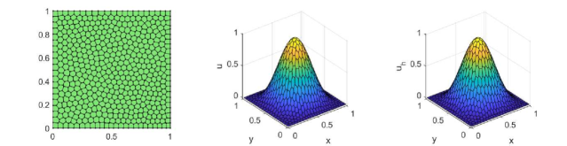
Fig. 1: Numerical and exact solutions for Example 5.2 ($\varepsilon=10^{-10}$)

Example 5.2.

The exact solution is given by $u=\sin(\pi x)^{2}\sin(\pi y)^{2}$.

Fig. 2: Convergence rate for Example 5.2 ($\varepsilon=10^{-10}$)

Fig. 1 displays the numerical solution and exact solution for $\varepsilon=10^{-10}$. These two figures fit well, and the optimal first-order convergence is still observed in Fig. 2 although the singular parameter $\varepsilon$ is very small.

6 Conclusion

We proposed a modified interior penalty virtual element method to solve the fourth-order singular perturbation problem. Drawing inspiration from the technique of the modified Morley element, we deduced optimal convergence in the energy norm and demonstrated robustness with the perturbation parameter in the lowest-order case.

CRediT authorship contribution statement

Fang Feng and Yue Yu collaborated closely to shape the conceptualization, methodology, and writing of this research. Additionally, Yue Yu took charge of implementing the discrete method in the study.

Declaration of competing interest

The authors declare that they have no known competing financial interests or personal relationships that could have appeared to influence the work reported in this paper.

Data availability

Data will be made available on request.

References

- [1] D. Adak and S. Natarajan. Virtual element method for semilinear sine-Gordon equation over polygonal mesh using product approximation technique. Math. Comput. Simulation, 172:224–243, 2020.
- [2] B. Ahmad, A. Alsaedi, F. Brezzi, L.D. Marini, and A. Russo. Equivalent projectors for virtual element methods. Comput. Math. Appl., 66(3):376–391, 2013.
- [3] S. N. Alvarez, L. Beirão Da Veiga, F. Dassi, V. Gyrya, and G. Manzini. The virtual element method for a 2D incompressible MHD system. Math. Comput. Simulation, 211:301–328, 2023.
- [4] P. F. Antonietti, L. Beirão da Veiga, and G. Manzini. The virtual element method and its applications. Springer, Cham, 2022.
- [5] P. F. Antonietti, M. Bruggi, S. Scacchi, and M. Verani. On the virtual element method for topology optimization on polygonal meshes: a numerical study. Comput. Math. Appl., 74(5):1091–1109, 2017.
- [6] P. F. Antonietti, G. Manzini, and M. Verani. The fully nonconforming virtual element method for biharmonic problems. Math. Models Methods Appl. Sci., 28(2):387–407, 2018.
- [7] L. Beirão Da Veiga, F. Brezzi, A. Cangiani, G. Manzini, L. D. Marini, and A. Russo. Basic principles of virtual element methods. Math. Models Meth. Appl. Sci., 23(1):199–214, 2013.
- [8] L. Beirão Da Veiga, F. Brezzi, L. D. Marini, and A. Russo. The Hitchhiker’s guide to the virtual element method. Math. Models Meth. Appl. Sci., 24(8):1541–1573, 2014.
- [9] L. Beirão Da Veiga, F. Dassi, G. Manzini, and L. Mascotto. The virtual element method for the 3D resistive magnetohydrodynamic model. Math. Models Methods Appl. Sci., 33(3):643–686, 2023.
- [10] L. Beirão Da Veiga, C. Lovadina, and G. Vacca. Virtual elements for the Navier-Stokes problem on polygonal meshes. SIAM J. Numer. Anal., 56(3):1210–1242, 2018.
- [11] L. Beirão Da Veiga, D. Mora, and G. Vacca. The Stokes complex for virtual elements with application to Navier–Stokes flows. J. Sci. Comput., 81:990–1018, 2019.
- [12] S. C. Brenner and M. Neilan. A interior penalty method for a fourth order elliptic singular perturbation problem. SIAM J. Numer. Anal., 49:869–892, 2011.
- [13] S. C. Brenner and L. R. Scott. The Mathematical Theory of Finite Element Methods. Springer, New York, 2008.
- [14] S. C. Brenner and L. Sung. interior penalty methods for fourth order elliptic boundary value problems on polygonal domains. J. Sci. Comput., 22/23:83–118, 2005.
- [15] F. Brezzi, A. Buffa, and K. Lipnikov. Mimetic finite differences for elliptic problems. M2AN Math. Model. Numer. Anal., 43(2):277–295, 2009.
- [16] F. Brezzi and L. D. Marini. Virtual element methods for plate bending problems. Comput. Methods Appl. Mech. Engrg., 253:455–462, 2013.
- [17] E. Cáceres and G. N. Gatica. A mixed virtual element method for the pseudostress-velocity formulation of the Stokes problem. IMA J. Numer. Anal., 37:296–331, 2017.
- [18] A. Cangiani, G. Manzini, and O. J. Sutton. Conforming and nonconforming virtual element methods for elliptic problems. IMA J. Numer. Anal., 37(3):1317–1354, 2016.
- [19] L. Chen and J. Huang. Some error analysis on virtual element methods. Calcolo, 55(1):5, 2018.
- [20] L. Chen and X. Huang. Nonconforming virtual element method for -th order partial differential equations in . Math. Comput., 89(324):1711–1744, 2020.
- [21] H. Chi, A. Pereira, I. F. M. Menezes, and G. H. Paulino. Virtual element method (VEM)-based topology optimization: an integrated framework. Struct. Multidiscip. Optim., 62(3):1089–1114, 2020.
- [22] C. Chinosi and L. D. Marini. Virtual element method for fourth order problems: -estimates. Comput. Math. Appl., 72(8):1959–1967, 2016.
- [23] B. A. De Dios, K. Lipnikov, and G. Manzini. The nonconforming virtual element method. ESAIM Math. Model. Numer. Anal., 50(3):879–904, 2016.
- [24] F. Feng, W. Han, and J. Huang. Virtual element method for an elliptic hemivariational inequality with applications to contact mechanics. J. Sci. Comput., 81(4036991):2388–2412, 2019.
- [25] F. Feng, W. Han, and J. Huang. A nonconforming virtual element method for a fourth-order hemivariational inequality in kirchhoff plate problem. J. Sci. Comput., 90(3):89, 24 pp., 2022.
- [26] G. N. Gatica and M. Munar. A mixed virtual element method for the Navier–Stokes equations. Math. Models Methods Appl. Sci., 28(14):2719–2762, 2018.
- [27] J. Huang and Y. Yu. A medius error analysis for nonconforming virtual element methods for poisson and biharmonic equations. J. Comput. Appl. Math., 386:113229, 20 pp, 2021.
- [28] M. Ling, F. Wang, and W. Han. The nonconforming virtual element method for a stationary Stokes hemivariational inequality with slip boundary condition. J. Sci. Comput., 85(3):Paper No. 56, 19, 2020.
- [29] X. Liu, J. Li, and Z. Chen. A nonconforming virtual element method for the Stokes problem on general meshes. Comput. Methods Appl. Mech. Engrg, 320:694–711, 2017.
- [30] T. K. Nilssen, X. Tai, and R. Winther. A robust nonconforming -element. Math. Comput., 70(234):489–505, 2001.
- [31] B. Philipp, C. Carsten, and S. Julian. Local parameter selection in the interior penalty method for the biharmonic equation. arXiv:2209.05221v2, 2023.
- [32] J. Qiu, F. Wang, M. Ling, and J. Zhao. The interior penalty virtual element method for the fourth-order elliptic hemivariational inequality. Commun. Nonlinear Sci. Numer. Simul., 127(4644807):Paper No. 107547, 17, 2023.
- [33] B. Semper. Conforming finite element approximations for a fourth-order singular perturbation problem. SIAM J. Numer. Anal., 29(4):1043–1058, 1992.
- [34] C. Talischi, G. H. Paulino, A. Pereira, and Ivan F. M. Menezes. Polymesher: a general-purpose mesh generator for polygonal elements written in matlab. Struct. Multidiscip. Optim., 45(3):309–328, 2012.
- [35] F. Wang and H. Wei. Virtual element method for simplified friction problem. Appl. Math. Lett., 85(3820290):125–131, 2018.
- [36] F. Wang, B. Wu, and W. Han. The virtual element method for general elliptic hemivariational inequalities. J. Comput. Appl. Math., 389(4194398):Paper No. 113330, 19, 2021.
- [37] F. Wang and J. Zhao. Conforming and nonconforming virtual element methods for a Kirchhoff plate contact problem. IMA J. Numer. Anal., 41(2):1496–1521, 2021.
- [38] M. Wang. On the necessity and sufficiency of the patch test for convergence of nonconforming finite elements. SIAM J. Numer. Anal., 39(2):363–384, 2001.
- [39] M. Wang, J. Xu, and Y. Hu. Modified Morley element method for a fourth order elliptic singular perturbation problem. J. Comput. Math., 24(2):113–120, 2006.
- [40] W. Xiao and M. Ling. Virtual element method for a history-dependent variational-hemivariational inequality in contact problems. J. Sci. Comput., 96(3):Paper No. 82, 21, 2023.
- [41] X. Zhang, H. Chi, and G. H. Paulino. Adaptive multi-material topology optimization with hyperelastic materials under large deformations: a virtual element approach. Comput. Methods Appl. Mech. Engrg., 370(4129484):112976, 34, 2020.
- [42] J. Zhao, S. Mao, B. Zhang, and F. Wang. The interior penalty virtual element method for the biharmonic problem. Math. Comp., 92(342):1543–1574, 2023.
- [43] J. Zhao, B. Zhang, and S. Chen. The nonconforming virtual element method for fourth-order singular perturbation problem. Adv. Comput. Math., 46(2):Paper No. 19, 23, 2020.
- [44] J. Zhao, B. Zhang, S. Chen, and S. Mao. The Morley-type virtual element for plate bending problems. J. Sci. Comput., 76(1):610–629, 2018.