Variable Importance in High-Dimensional Settings Requires Grouping

Abstract

Explaining the decision process of machine learning algorithms is nowadays crucial for both a model’s performance enhancement and human comprehension. This can be achieved by assessing the variable importance of single variables, even for high-capacity non-linear methods, e.g. Deep Neural Networks (DNNs). While only removal-based approaches, such as Permutation Importance (PI), can bring statistical validity, they return misleading results when variables are correlated. Conditional Permutation Importance (CPI) bypasses PI’s limitations in such cases. However, in high-dimensional settings, where high correlations between the variables cancel their conditional importance, the use of CPI as well as other methods leads to unreliable results, besides prohibitive computation costs. Grouping variables statistically via clustering or some prior knowledge gains some power back and leads to better interpretations. In this work, we introduce BCPI (Block-Based Conditional Permutation Importance), a new generic framework for variable importance computation with statistical guarantees handling both single and group cases. Furthermore, as handling groups with high cardinality (such as a set of observations of a given modality) are both time-consuming and resource-intensive, we also introduce a new stacking approach extending the DNN architecture with sub-linear layers adapted to the group structure. We show that the ensuing approach extended with stacking controls the type-I error even with highly-correlated groups and shows top accuracy across benchmarks. Furthermore, we perform a real-world data analysis in a large-scale medical dataset where we aim to show the consistency between our results and the literature for a biomarker prediction.

1 Introduction

Machine Learning (ML) algorithms are extensively used in many fields of science, such as biomedical application (Strzelecki and Badura 2022; Alber et al. 2019), neuroscience (Kora et al. 2021; Knutson and Pan 2020), and social sciences (Lundberg, Brand, and Jeon 2022; Chen et al. 2021). The increasing importance of ML in society raises issues of accountability, hence, stimulating research on interpretable ML. Reaching a comprehensive understanding of the decision process is crucial for providing statistical and, ideally, scientific insights to the practitioner (Gao et al. 2022; Molnar et al. 2021a; Fleming 2020; Hooker et al. 2019).

To gauge the impact of variables on model prediction, aka variable importance, several model-agnostic attempts have emerged (Molnar 2022; Ribeiro, Singh, and Guestrin 2016). Examples include Permutation Feature Importance (PFI) (Breiman 2001), Conditional Randomization Test (Candes et al. 2017) and Leave-One-Covariate-Out (LOCO) (Lei et al. 2018). All these instances constitute removal-based approaches (Covert, Lundberg, and Lee 2020), and are so far, the only ones known to provide statistically grounded measures of significance. Importantly, removal-based approaches require retraining the model after removing the variable of interest and are, therefore, time-consuming. Moreover, the common Permutation Importance (PI, Breiman 2001) risks mistaking insignificant variables for significant ones when variables are correlated (Hooker, Mentch, and Zhou 2021). Conditional Permutation Importance CPI can overcome these limitations (Blesch, Watson, and Wright 2023; Watson and Wright 2021; Debeer and Strobl 2020; Fisher, Rudin, and Dominici 2019; Chamma, Engemann, and Thirion 2023). However, in high-dimensional settings, single variable importance computation suffers from very high correlation between the variables (Chevalier et al. 2021). More precisely, this makes conditional importance estimation less informative, as it remains unclear how much information each variable adds. In the extreme case where variables are duplicated, conditional importance can no longer be defined. More generally, correlations larger than $.8$ are known to present a hard challenge, at least for linear learners (Chevalier et al. 2021). Importance analysis then typically yields spuriously significant variables, which ruins its ability to statistically control the false positive rate (Strobl et al. 2008). Besides, examining the importance of each of the hundreds or thousands variables separately will result in prohibitive computation costs (Covert, Lundberg, and Lee 2020) —removal procedures typically have quadratic complexity— and defy model interpretability.

Group-based analysis can offer a remedy at it regularizes power estimates and leads to reduced computation time (Molnar et al. 2021b; Bühlmann 2013). This can improve inference as it helps handle the curse of correlated variables in high-dimensional settings. So far, common group-based methods neglected investigating statistical guarantees, in particular, type-I error control, i.e. the percentage of irrelevant variables identified as relevant (false positives). Statistical error control for groups obviously requires information on variable grouping available through two strategies: Knowledge-driven grouping, where the variables are grouped based on their domain-specific information rather than their shared statistical properties and Data-driven grouping, where clustering approaches are used such as hierarchical or divisive clustering.

Grouping has also been successfully performed for multimodal applications  (Albu, Bocicor, and Czibula 2023; Engemann et al. 2020; Rahim et al. 2015) via model stacking (Wolpert 1992) which is typically based on pipelines of disconnected models.

Contributions

We propose Block-Based Conditional Permutation Importance (BCPI), a new framework for variable importance computation (single and group levels) with explicit statistical guarantees (p-values).

• Following our review of the literature (section 2), we provide theoretical results on group-based conditional permutation importance (section 3.2).

• We propose a novel internal stacking approach by extending the architecture of our default Deep Neural Network (DNN) model with the use of a linear projection of the groups, which can significantly reduce computation time (section 3.3).

• We conduct extensive benchmarks on synthetic and real world data (section 4) which demonstrate the capacity of the proposed method to combine high prediction performance with theoretically grounded identification of predicatively important groups of variables.

• We provide publicly available code (compatible with the Scikit-learn API) on GitHub (https://github.com/achamma723/Group˙Variable˙Importance).

2 Related work

Group-based variable importance has been introduced for Random Forests by (Wehenkel et al. 2018), extending the seminal work of Louppe et al. (2013) on Mean Decrease Impurity (MDI). Once all the variables have their corresponding impurity function scores, the importance score of the group of interest are ($1$) the sum, ($2$) the average or ($3$) the maximum of the impurity scores among the participating variables. Despite that, ($1$) the sum displays bias in favor of larger-sized groups, ($2$) the average diminishes a group’s significance when only a small fraction of its features hold importance and ($3$) the maximum suggests that the sole most important feature reflects the collective importance of the group.

Williamson et al. (2021) proposed a model-agnostic approach based on refitting the learner after the removal of a variable of interest also called LOCO (Leave-One-Covariate-Out) by Lei et al. (2018). This work has then been adapted to the group-level by considering the removal of all the variables of the group of interest jointly, as in Leave-One-Group-Out (LOGO) presented in (Au et al. 2021). In lieu of removing the group of interest, Au et al. (2021) established Leave-One-Group-In (LOGI) that assesses the impact of the group of interest on the prediction compared to the null model - the prediction is the average of the outcome. However, this approach becomes intractable easily due to the necessity of refitting the learner for each group, particularly in the case of low cardinality groups.

Mi et al. (2021) proposed an efficient model-agnostic procedure for black-box models’ interpretation. It uses the permutation approach (Breiman 2001; Fisher, Rudin, and Dominici 2019) with the importance score computed as the reduction in a model’s performance when randomly shuffling the variable of interest. To account for group-level structure, (Gregorutti, Michel, and Saint-Pierre 2015) suggested taking into account all the variables of the group of interest in the permutation scheme jointly, known as Group Permutation Feature Importance (GPFI). Au et al. (2021) proposed Group Only Permutation Feature Importance (GOPFI) which examines the level of the group’s individual contribution to the model’s performance. The random joint shuffling is performed for all the variables of the different groups expect the ones of the group of interest. However, according to Strobl et al. (2008), simple permutation approaches yield poor accuracy and specificity in high correlation settings. Lee, Sood, and Craven (2018) applied perturbations to the variables and groups of interest while providing p-values. Nevertheless, they did not focus on the degree of correlation between the variables (and the groups) which increases the difficulty of the problem.

A different angle can be motivated by a recent line of work that developed model-stacking techniques (Wolpert 1992) which combine different input domains and groups of variables rather than aggregating different estimators on the input data. This approach has been used in various applications ranging from video analysis (Zhou et al. 2021) over protein-protein interactions (Albu, Bocicor, and Czibula 2023) to neuroscience applications (Rahim et al. 2015). A key benefit of multimodal or group stacking is that it allows for modality-specific encoding strategies and while approaching inference at the simplified level of the 2^nd level model combining the modality-wise predictions or activations. This strategy has been used to explore importance of distinct types of brain activity at different frequencies for age prediction (Sabbagh et al. 2023; Engemann et al. 2020). While stacking is easy to implement with standard software e.g. scikit-learn (Pedregosa et al. 2011), inference with stacking has not been formalized yet. Moreover, it requires fitting multiple disconnected estimators which may limit the capacity of the model.

3 BCPI and Internal Stacking Approach

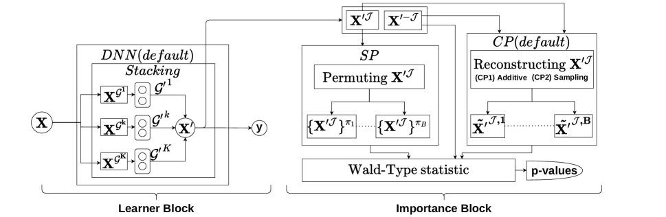
Figure 1: Block-Based Conditional Permutation Importance: Framework for single/group variable importance computation with statistical guarantees. (Learner Block) The learner used to predict the outcome $\mathbf{y}$ from the design matrix $\mathbf{X}$. Internal stacking linearly projects each group by the mean of an extra linear sub-layer. (Importance Block): Reconstruction of the group of interest $\mathbf{X^{\prime\mathcal{J}}}$ is accomplished via CP (Conditional Permutation) block with (CP1) the additive or (CP2) the sampling constructions as stated in section 3.2. The permutation scheme can be changed to standard permutation (SP).

3.1 Preliminaries

Notations

We denote by matrices, vectors, scalar variables and sets by bold uppercase letters, bold lowercase letters, script lowercase letters, and calligraphic letters, respectively (e.g. $\mathbf{X}$, $\mathbf{x}$, $x$, $\mathcal{X}$). Designating by $\mu$ the function that maps the sample space $\mathcal{X}\subset\mathbb{R}^{p}$ to the outcome space $\mathcal{Y}\subset\mathbb{R}$ and $\hat{\mu}$ is an estimate of $\mu$ within a certain class $\mathcal{F}$ of estimators. We express by $\llbracket n\rrbracket$ the set {1, …, $n$}, by $\langle.,.\rangle$ the standard dot product and by ($\pi$) the shuffling process.

Let $\mathcal{S}=\{\mathcal{G}^{k},k\in\llbracket K\rrbracket\}$ and $\mathcal{S^{\prime}}=\{\mathcal{G^{\prime}}^{k},k\in\llbracket K\rrbracket\}$ be the set of $K$ pre-defined subset of variables in the data and the set of $K$ new subset of variables following linear projections with a set $\mathcal{P}$ of projection matrices, respectively. Projection matrices are meant to produce a group summary of the information. Let $\mathcal{P}=\{\mathbf{U_{k}},k\in\llbracket K\rrbracket\}$ be the set of projection matrices $\mathbf{U_{k}}\in\mathbb{R}^{|\mathcal{G}^{k}|\times|\mathcal{G^{\prime}}^{k}|}$. Let $\mathcal{J}=\{j_{1},\dots,j_{r}\}\in(\mathcal{S}\cup\mathcal{S^{\prime}})$ be a subset of $r$ variables with consecutive indices in $\llbracket p\rrbracket$, $r\leq p$. Let $\mathbf{X}\in\mathbb{R}^{n\times p}$ be a design matrix where $i^{th}$ row, $j^{th}$ column and $\mathcal{J}^{th}$ subset of columns are indicated by $\mathbf{x_{i}}$, $\mathbf{x^{j}}$ and $\mathbf{X^{\mathcal{J}}}$ respectively. Let $\mathbf{X^{\mathcal{-J}}}=(\mathbf{x^{1}},\dots,\mathbf{x^{j_{1}-1}},\mathbf{x^{j_{r}+1}},\dots,\mathbf{x^{p}})$ be the design matrix with the $\mathcal{J}^{th}$ subset of variables is removed. Let $\mathbf{X^{\mathcal{(J)}}}=(\mathbf{x^{1}},\dots,\mathbf{x^{j_{1}-1}},\{\mathbf{x^{j_{1}}}\}^{\pi},\dots,\{\mathbf{x^{j_{r}}}\}^{\pi},\dots,\mathbf{x^{p}})$ be the design matrix with the $\mathcal{J}^{th}$ subset of variables is shuffled. The rows of $\mathbf{X^{\mathcal{-J}}}$ and $\mathbf{X^{(\mathcal{J})}}$ are denoted $\mathbf{x_{i}^{\mathcal{-J}}}$ and $\mathbf{x_{i}^{\mathcal{(J)}}}$ respectively, for $i\in\llbracket n\rrbracket$. Let $\mathbf{X^{\prime}}$ be the linearly projected version of $\mathbf{X}$ via $\mathcal{P}$ where $p^{\prime}=\sum_{k=1}^{K}|\mathcal{G^{\prime}}^{k}|$.

Problem Setting

We consider the regression or the classification problem where the response vector $\mathbf{y}\in\mathbb{R}^{n}$ or $\in\{0,1\}^{n}$ respectively and the design matrix $\mathbf{X}\in\mathbb{R}^{n\times p}$ (encompasses $n$ observations of $p$ variables), along with $\mathcal{S}$ (i.e. $K$ pre-defined groups). Across the paper, we rely on an i.i.d. sampling train/validation/test partition scheme where the $n$ samples are divided into $n_{train}$ training and $n_{test}$ test samples. The train samples were used to train $\hat{\mu}$ with empirical risk minimization. This function is utilized for appraising the importance of variables on a novel dataset (test set).

3.2 Group conditional variable importance

We define the joint permutation of group $\mathbf{x}^{\mathcal{J}}$ conditional to $\mathbf{x^{-\mathcal{J}}}$, as a group $\mathbf{\tilde{x}^{\mathcal{J}}}$ that preserves the joint dependency of $\mathbf{x^{\mathcal{J}}}$ with respect to the other variables in $\mathbf{x^{-\mathcal{J}}}$, although the independent part is shuffled. The reconstruction of $\mathbf{\tilde{x}^{\mathcal{J}}}$ is done via two approaches, both, based on fast approximation with a lean model: (1) Additive construction combines the prediction of a Random Forest using the remaining groups and a shuffled version of the residuals i.e. $\mathbf{\tilde{x^{\prime}}}^{\mathcal{J}}=\mathbb{E}(\mathbf{{x^{\prime}}^{\mathcal{J}}}|\mathbf{{x^{\prime}}^{\mathcal{-J}}})+(\mathbf{{x^{\prime}}^{\mathcal{J}}}-\mathbb{E}(\mathbf{{x^{\prime}}^{\mathcal{J}}}|\mathbf{{x^{\prime}}^{\mathcal{-J}}}))^{\pi}$ where the residuals of the regression of $\mathbf{{x^{\prime}}^{\mathcal{J}}}$ on $\mathbf{{x^{\prime}}^{\mathcal{-J}}}$ are shuffled. (2) Sampling construction uses a Random Forest model to fit $\mathbf{{x^{\prime}}^{\mathcal{J}}}$ from $\mathbf{{x^{\prime}}^{\mathcal{-J}}}$, followed by sampling the prediction from within its leaves. When dealing with regression, this results in the following importance estimator:

$$\hat{m}^{\mathcal{J}}_{CPI}=\frac{1}{n_{test}}\sum_{i=1}^{n_{test}}\left((y_{i}-\hat{\mu}(\mathbf{\tilde{x}_{i}^{(\mathcal{J})}}))^{2}-(y_{i}-\hat{\mu}(\mathbf{x_{i}}))^{2}\right),$$ (1)

where $\mathbf{\tilde{X}^{(\mathcal{J})}}=(\mathbf{x^{1}},\dots,\mathbf{x^{j_{1}-1}},\mathbf{\tilde{x}^{j_{1}}},\dots,\mathbf{\tilde{x}^{j_{r}}},\\ \dots,\mathbf{x^{p}})\in\mathbb{R}^{n_{test}\times p}$ be the new design matrix including the remodeled version of the group of interest $\mathbf{X^{\mathcal{J}}}$.

In Fig. 1, we introduce BCPI a novel general framework for variable importance, at both single and group levels, yielding statistically valid p-values. It consists of two blocks: a Learner Block defined by the prediction model of interest Importance Block reconstructing the variable (or group) of interest via conditional permutation (CP) – $\hat{m}^{\mathcal{J}}_{CPI}$. The implementation provided with this work supports estimators compatible with the scikit-learn API for both blocks. Yet, our default method BCPI-DNN is adapted with: (1) a DNN as a base learner for its high predictive capacity inspired from (Mi et al. 2021) and (2) a Random Forest, a less powerful, but much simpler, yet, still generic model as a conditional probability learner. For study purposes, the framework is also adapted with the standard permutation scheme through the (SP) block (labeled BPI). The theoretical results, conditions underlying this proposition as well as limitations of (PI) were developed in (Chamma, Engemann, and Thirion 2023) and adapted to the group setting (supplementary materials).

Proposition.

Assuming that the estimator $\hat{\mu}$ is obtained from a class of functions $\mathcal{F}$ with sufficient regularity, i.e. that it meets conditions of A1: optimality, A2: differentiability, A3: continuity of optimization, A4: Continuity of derivative, B1: Minimum rate of convergence and B2: Limited complexity, the importance score $\hat{m}^{\mathcal{J}}_{CPI}$ defined in (1) cancels when $n_{train}\rightarrow\infty$ and $n_{test}\rightarrow\infty$ under the null hypothesis, i.e. the $\mathcal{J}^{th}$ group is not significant for the prediction. Moreover, the Wald statistic $z^{\mathcal{J}}=\frac{mean(\hat{m}^{\mathcal{J}}_{CPI})}{std(\hat{m}^{\mathcal{J}}_{CPI})}$ obtained by dividing the mean of the importance score by its standard deviation asymptotically follows a standard normal distribution.

This implies that in the large sample limit, the p-value associated with $z^{\mathcal{J}}$ controls the type-I error rate for all optimal estimators in $\mathcal{F}$. It entails making sure that the importance score defined in (1) is 0 for the class of learners that meet specific convergence guarantees and are immutable to arbitrary change in their $\mathcal{J}^{th}$ arguments, conditional on the others. We also state the precise technical conditions under with $\hat{m}^{\mathcal{J}}_{CPI}$ used is (asymptotically) valid, i.e. leads to a Wald-type statistic that behaves as a standard normal under the null hypothesis. As a result, all terms in Eq. 1 vanish with speed $\frac{1}{\sqrt{n_{test}}}$ from the Berry-Essen theorem, under the assumption that the test samples are i.i.d.

3.3 Internal Stacking

The vector $\mathbf{x}\in\mathcal{X}$ is composed of $K$ groups in $\mathcal{S}$, each considered as an independent input modality. Performing column slicing on $\mathbf{x}$, according to $\mathcal{S}$, yields the set $\{\mathbf{x^{\mathcal{G}^{k}}},k\in\llbracket K\rrbracket\}$. A linear transformation to a lower space is applied on each input modality $\mathbf{x^{\mathcal{G}^{k}}}$ through the set of projection matrices $\mathcal{P}$ producing a linear variant denoted $\mathbf{x^{\prime k}}$ as:

$$\mathbf{{x^{\prime}}^{k}}=<\mathbf{x^{\mathcal{G}^{k}}},\mathbf{U_{k}}>,$$

where $k\in\llbracket K\rrbracket$.

Concatenating the set of linear variants $\{\mathbf{{x^{\prime}}^{k}},k\in\llbracket K\rrbracket\}$ provides the linear version of $\mathbf{x}$ i.e. the vector $\mathbf{x^{\prime}}$. If the new space is a unidimensional Euclidean space i.e. $\mathbf{{x^{\prime}}}\in\mathbb{R}^{K}$, a group summary of the information within all groups is returned, and the problem is reduced to the single-level case. However, if the new space is not unidimensional, we then have a dimension reduction, where the group summary of information is exclusive per group (multioutputs per group). In this case, the new groups contained in $\mathbf{x}$ are denoted $\mathcal{G^{\prime}}^{k}$ with the corresponding linear variant $\mathbf{x^{\prime}}^{\mathcal{G^{\prime}}^{k}}$ as seen in Fig. 1. Instead of performing stacking in a separate estimation step under a different learner, we have incorporated it to the inference process, thus learning a consistent new presentation of the groups. This is simply implemented as an initial linear sub-layer without activation in the $\hat{\mu}$ network. Therefore, $\mathbf{{x^{\prime}}^{k}}$ can be seen analogous to the predictions from the input models in a classical stacking pipeline that are forwarded to the meta learner, hence, $\mathbf{{x^{\prime}}^{k}}$ can be treated like a regular data column by permutation algorithms.

4 Experiments

To ensure a fair comparison across experiments, we use all methods with their original implementation. As for BCPI-DNN, BCPI-RF and BPI-DNN particularly, the default behavior consists of a 2-fold internal cross validation where the importance inference is performed on an unseen test set. The scores from different splits are thus concatenated to compute the final variable importance. All experiments are performed with $100$ runs.

4.1 Experiment 1: Benchmark of grouping methods

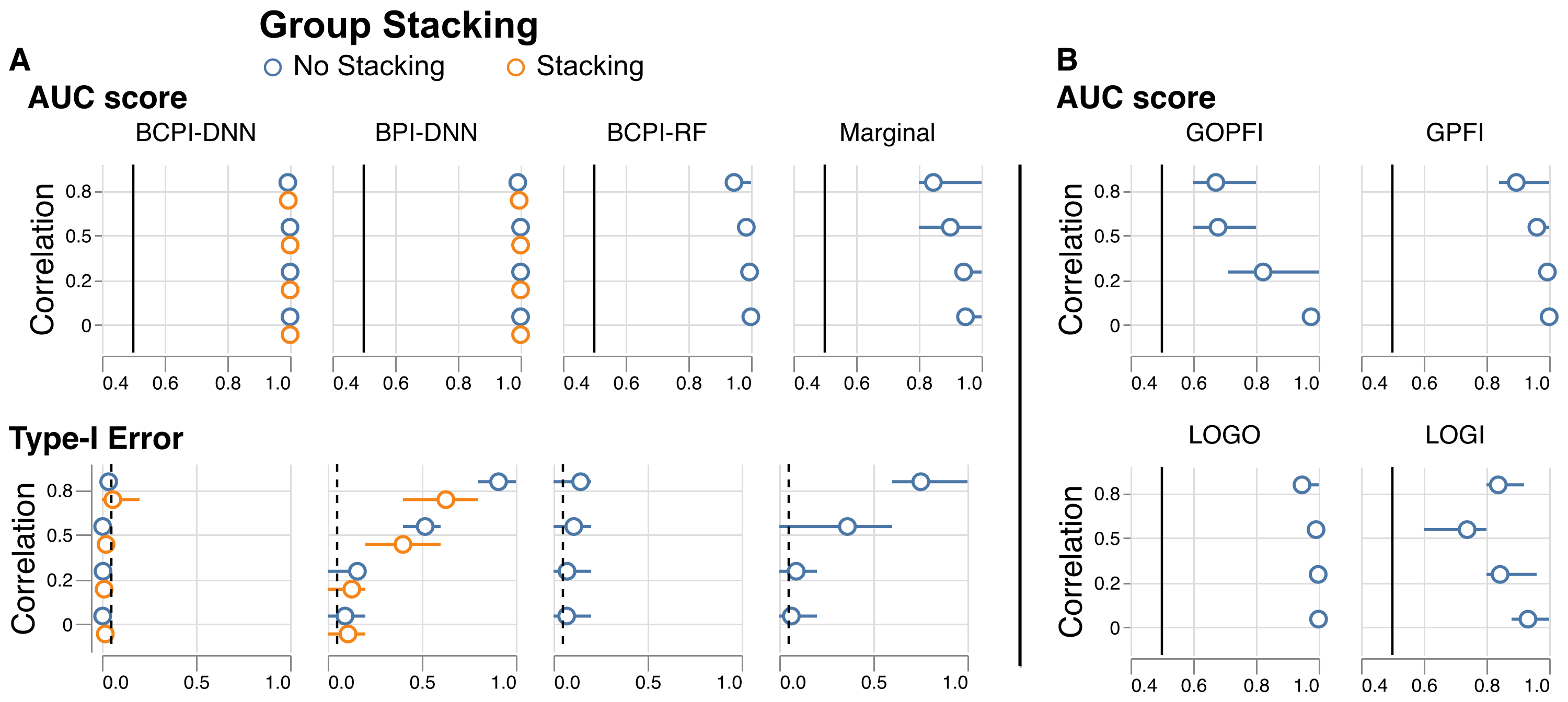
Figure 2: Benchmarking grouping methods: BCPI-DNN is compared to baseline models and competing approaches for group variable importance. (A) AUC score (correct ranking of variables) and Type-I error ($\text{p-val}<0.05$) for methods providing p-values. (B) AUC scores for methods not providing p-values. Prediction tasks were simulated with $n$ = $1000$ and $p$ = $50$. Dashed line: targeted type-I error rate at 5%. Solid line: chance level.

We include BCPI-DNN in a benchmark with other state-of-the-art methods for group-based variable importance. The data $\{\mathbf{x_{i}}\}_{i=1}^{n}$ follow a Gaussian distribution with a predefined covariance structure $\mathbf{\Sigma}$ i.e. $\mathbf{x_{i}}\sim\mathcal{N}(0,\mathbf{\Sigma})\forall i\in\llbracket n\rrbracket$. We consider a block-designed covariance matrix $\mathbf{\Sigma}$ of $10$ blocks with an intra-block correlation coefficient $\rho_{intra}=0.8$ among the variables of each block and an inter-block correlation coefficient $\rho_{inter}\in\{0,0.2,0.5,0.8\}$ between the variables of the different blocks. Each block is considered as a separate group. In this experiment, $n=1000$ and $p=50$ i.e. we have 5 variables per block/group. We defined an important group as a group having at least one variable that took part in simulating the outcome $y$. Thus, to predict $y$, we rely on a linear model where the first variable of each of the first 5 groups is used in the following model:

$$y_{i}=\mathbf{x_{i}}\bm{\beta}+\sigma\epsilon_{i},\forall i\in\llbracket n\rrbracket$$ (2)

where $\bm{\beta}$ is a vector of regression coefficients having only $5$ non-zero coefficients (the true model), $\bm{\epsilon}\in\mathcal{N}(0,\mathbf{I})$ is the Gaussian additive noise with magnitude $\sigma=\frac{||\mathbf{X}\bm{\beta}||_{2}}{SNR\sqrt{n}}$. We used the same setting from (Janitza, Celik, and Boulesteix 2018) where the $\bm{\beta}$ values are drawn i.i.d. from the set $\mathcal{B}=\{\pm 3,\pm 2,\pm 1,\pm 0.5\}$. We consider the following state-of-the-art baselines:

• Marginal Effects: A multivariate linear model is applied to each group separately. Importance scores correspond to ensuing p-values.

• Leave-One-Group-In (LOGI) (Au et al. 2021): Similar to Marginal Effects using a Random Forest. Provides no p-values.

• Leave-One-Group-Out (LOGO) (Williamson et al. 2021): Refitting of the model is performed after removing the group of interest.

• Group Only Permutation Feature Importance (GOPFI) (Au et al. 2021): Joint permutation of all variables except for those of the group of interest.

• Group Permutation Feature Importance (GPFI) (Gregorutti, Michel, and Saint-Pierre 2015; Valentin, Harkotte, and Popov 2020): Joint permutation of all variables of the group of interest.

In addition, we benchmarked the three variants of our proposed method:

• BPI-DNN: Similar to GPFI based on a DNN estimator. It is also enhanced by the new internal stacking approach.

• BCPI-RF: BCPI where $\hat{\mu}$ is obtaind from a Random Forest.

• BCPI-DNN: BCPI where $\hat{\mu}$ is a DNN. It is also enhanced by the new internal stacking approach.

4.2 Experiment 2: Impact of Stacking

To assess the impact of performing stacking regarding accuracy in inference and computation time, we conducted a comparison restricted to BCPI-DNN. We relied on the same covariance structure setting as in Experiment $1$ with an intra-block correlation coefficient $\rho_{intra}=0.8$ and an inter-block correlation coefficient $\rho_{inter}=0.8$. The number of samples $n$ and the number of variables $p$ were both set to $1000$ i.e. the number of variables per block/group increased to 100 in order to build groups with high cardinality. The outcome $y$ was simulated using the same model as in Eq. 2 where a group is predefined as important having at least $10\%$ of its variables taking part in computing the outcome.

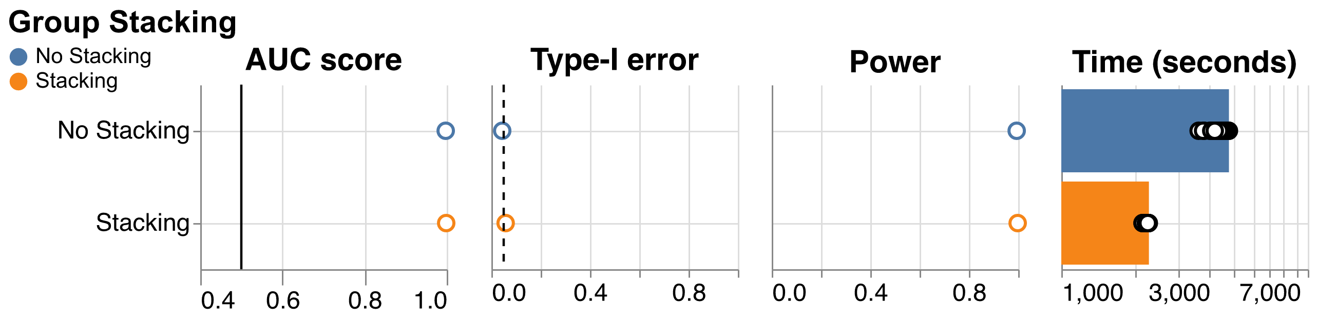
Figure 3: Impact of Stacking: Performance at detecting important groups on simulated data with $n$ = $1000$ and $p$ = $1000$ with $10$ blocks/groups, each group having a cardinality of $10$. AUC scores and Type-1 error as in Fig. 2. (Power) quantifies the average proportion of detected informative variables ($\text{p-value}<0.05$). Panel (Time) displays computation time in seconds with $\log_{10}$ scale per core on $100$ cores. Dashed line: targeted type-I error rate. Solid line: chance level.

4.3 Experiment 3: Age prediction with UKBB

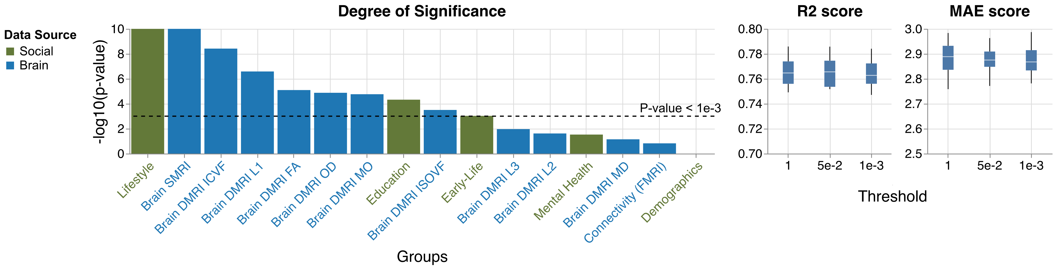
Figure 4: Brain Age prediction in UKBB: Prediction of brain age from various socio-demographic and brain-imaging groups of phenotypes in a sample of $n$ = $8357$ volunteers from the UK BioBank. (Degree of significance) plots the level of significance for the different brain (in blue) and social (in red) groups in terms of $-\log_{10}$ of the derived p-values. Dashed line: targeted type-I error rate at $p=0.001$. (R2 score & MAE score) checks the performance of the trained learner when retaining all the groups vs removing non-significant groups.

We conducted an empirical benchmark of the performance of BCPI-DNN combined with internal stacking in a real-world biomedical dataset. The UK Biobank project (UKBB) encompasses imaging and socio-demographic derived phenotypes from a prospective cohort of participants drawn from the population of the UK (Constantinescu et al. 2022; Littlejohns et al. 2020). In the past years, the UKBB dataset has enabled large-scale studies investigating associations between various phenotypes (physiological, cognitive) and environmental or life-style factor. This has given rise to successful analysis of factors associated to personal well-being and health (Newby et al. 2021; Mutz and Lewis 2021) at an epidemiological scale. In the context of machine learning with brain data, age-prediction is an actively studied task which can provide a normative score when applying a reference model on clinical cohorts (Cole and Franke 2017). State-of-the-art models were based on convolutional neural networks and report mean absolute errors between 2-3 years (Roibu et al. 2023; Jonsson et al. 2019). Recent extensions have focused on MRI-contrast and region-specific insights, often based on informal inference (Roibu et al. 2023; Popescu et al. 2021). Another line of work (Dadi et al. 2021; Anatürk et al. 2021) has focused on other sources of normative ageing information, highlighting cognitive social and lifestyle factors. In this context, the analysis of importance of multimodal inputs has so far been hampered by the lack of formal inference procedures and the high-dimensional setting with highly correlated variables.

We approached this open task using the proposed method, reusing the pre-defined groups in the work by (Dadi et al. 2021). We focused on data from participants who attended the imaging visit ($n$ = $8357$) to study the group-level importance rankings provided by BCPI-DNN. We defined important groups by p-value threshold of $<10^{-3}$. While this setting lacks an explicit ground truth for the important groups, we explored the appropriate group selection through model performance in terms of ($R^{2}$ & MAE scores, 10-fold cross-validation) after removing the non-significant groups. We accessed the UKBB data through its controlled access scheme in accordance with its institutional ethics boards (Bycroft et al. 2018; Sudlow et al. 2015).

5 Results

We benchmarked state-of-the-art baselines and the proposed methods across data-generating scenarios under increasing inter-block correlation strength {0, 0.2, 0.5, 0.8} (Fig. 2). BCPI-DNN and BPI-DNN were implemented in two variants: with or without the novel internal stacking. For the AUC score, we observed that (BCPI-DNN & BPI-DNN - based on the DNN) and (BCPI-RF, GPFI & LOGO - based on Random Forests) showed the highest performance across the different scenarios, hence, accurately ordering the variables according to their significance. As expected, the Marginal baseline performed lowest as it could not access any conditional information. GOPFI and LOGI both suffered when the correlation between the groups increased, which is not surprising. Considering false positive rate, BCPI-DNN controlled the type-I error at the targeted rate (5 %) while BPI-DNN— based on the standard permutation of the group of interest— failed to do so in the setting of high correlations between the groups, and thus provided spurious results. Interestingly, for BPI-DNN, internal stacking slightly increased its capacity to control the type-I error. BCPI-RF— based on the conditional importance with Random Forests— better controlled the type-I error compared to BPI-DNN. Nevertheless, in the presence of strong correlations, it did not fully reach the target rate. Additional analyses suggested that the marginal approach failed in the current setting, whereas on average, the DNN had higher scores ($R^{2}\sim 0.95$) than the Random Forest ($R^{2}\sim 0.8$). Additional analyses of performance in terms of power and computation time of showed that BCPI-DNN, BPI-DNN, BCPI-RF and Marginal showed favorable results compared to other baselines and competing methods.

The AUC score, type-I error, power and computation time for Experiment 4.2 are presented in Fig. 3. BCPI-DNN with internal stacking performed similarly as the same approach without stacking. Thus, both approaches showed comparable inferential behavior in identifying the significant groups. Nevertheless, in terms of computation time, the dimension reduction brought by stacking added significant benefits (around a factor of 2). In fact, in the importance block without stacking, all the variables of the remaining groups are used to predict those of the group of interest. Groups with high cardinality (of variables) are challenging in terms of memory resources and required computation, suggesting that internal stacking can help to reduce computational burden. Real-world empirical application of BCPI-DNN with internal stacking for age-prediction from brain imaging and socio-demographic information are summarized in Fig. 4. Results in (Degree of Significance) ranked the groups according to their corresponding level of significance. We choose a conservative significance level of $p=0.001$ (Dashed line at $log_{10}(0.0001)=3$). Using the stacking approach, we scored the heterogeneous brain and social input variables regarding their predictive importance. As expected, we found that the brain groups - excluding Brain DMRI MD - were highly important for age prediction. Interestingly, Lifestyle and Education were among the top predictive variables, conditional on the brain groups, suggesting the presence of complementary information. To challenge the plausibility of the selected groups, we investigated prediction performance after excluding non-significant groups. We used 10-fold cross validation with significance estimation and refitting the reduced model using the training set while scoring with the reduced model on the testing set. The reduced model did not perform visibly worse than the full model ($R^{2}=0.8,MAE=2.9$), suggesting that our procedure effectively selects predictive groups. Of note the performance is in line with state-of-the art benchmarks on the UKBB based on convolutional neural networks ($MAE\sim$ 2-3 years, e.g., Roibu et al. 2023; Jonsson et al. 2019). Consequently, results suggest that the proposed approach combined good prediction performance with effective identification of relevant groups of variables. For additional supporting results, see supplementary materials.

6 Discussion

In this work, we proposed BCPI, a novel and usable framework for computing single- and group-level variable importance. Our work provides statistical guarantees based on results from Conditional Permutation Importance (CPI), whereas our implementation supports arbitrary regression and classification models consistent with the scikit-learn API. We developed our approach beginning from the observation that standard Permutation Importance PI, represented by the BPI-DNN approach, lacks the ability to control type-I error (Williamson et al. 2021) with high correlated settings in Fig. 2, despite the high AUC score (Mi et al. 2021). We extended these results, theoretically and empirically, to the group setting by proposing BCPI-DNN, which is built on top of an expressive DNN model as a base learner. This recipe led to high AUC scores while maintaining the control of type-I error across different correlation scenarios (Fig. 2).

Inspired by recent applications of model stacking for handling multiple groups or input domains (Albu, Bocicor, and Czibula 2023; Zhou et al. 2021; Engemann et al. 2020), we proposed internal stacking which implements stacking inside the DNN model, hence, avoids separate optimization problems common for stacking pipelines. This was achieved through extra sub-linear layers building linear summaries for each group of variables. Our benchmarks suggested that stacking maintained inferential performance of the full model while bringing time benefits (at least up to a factor of 2), especially for groups with high cardinality of variables (Fig. 3). Moreover, additional analyses of calibration of BCPI-DNN versus BPI-DNN suggested that the p-values for BCPI-DNN showed a slightly conservative profile for BCPI-DNN. Instead, BPI-DNN showed poor calibration, once more underlining the relevance of conditional permutations.

Our empirical investigation of age prediction using the UKBB dataset suggests that the proposed framework facilitates constructing strong predictions models alongside trustworthy insights on the important predictive inputs. While prediction performance of our model was in line with state-of-the art results for the UKBBRoibu et al. (2023); Jonsson et al. (2019)), here, we provided a statistically grounded confirmation for the conclusions drawn in Dadi et al. 2021 who used a less formal approach consistent with the LOGI approach.

Several limitations apply to our work. BCPI-DNN utilizes a DNN model as the base estimator for its high predictive accuracy. However, when the amount of training data is limited, the network can potentially memorize the training examples instead of learning generalizable patterns and a simpler base learner might be preferable, e.g. a Random Forest. Additional analyses of computation time for BCPI-DNN in situations of low ($5$) versus high ($100$) cardinality showed that the benefit of internal stacking became more pronounced with larger groups of variables. This is due to the extra training of the added sub-linear layers. Our work made use of predefined groups, which may not always be available. Instead, statistically defined groups could be used e.g. obtained from clustering. A possible issue might then be that the groups mix heterogeneous variables, which makes their interpretation challenging. Furthermore, it is important to apply one-hot encoding of categorical variables after clustering. On the flip side, reliance on predefined groups may lead to poor inference if the group structure does not track variable importance, e.g. if important variables are distributed in all groups. This topic deserves careful investigation in the future. Moreover, here we only performed internal stacking by applying linear projection on the input data. It will be interesting to better understand the potential of non-linear projections.

Finally, additional possible future directions include studying the impact of missing and low values on the accuracy, also across different group definitions.

Acknowledgement

This work has been supported by Bertrand Thirion and is supported by the KARAIB AI chair (ANR-20-CHIA-0025-01), and the H2020 Research Infrastructures Grant EBRAIN-Health 101058516. D.E. is a full-time employee of F. Hoffmann-La Roche Ltd.

Appendix A Conditional Permutation Importance (CPI) Wald statistic asymptotically controls type-I errors: hypotheses, theorem and proof

Outline

The proof relies on the observation that the importance score defined in (1) is $0$ in the asymptotic regime, where the permutation procedure becomes a sampling step, under the assumption that the subset of variables $\mathcal{J}$ is not conditionally associated with $y$. Then all the proof focuses on the convergence of the finite-sample estimator to the population one. To study this, we use the framework developed in (Williamson et al. 2021). Note that the major difference with respect to other contributions (Watson and Wright 2021) is that the ensuing inference is no longer conditioned on the estimated learner $\hat{\mu}$. Next, we first restate the precise technical conditions under which the different importance scores considered are asymptotically valid, i.e. lead to a Wald-type statistic that behaves as a standard normal under the null hypothesis.

Notations

Let $\mathcal{F}$ represent the class of functions from which a learner $\mu:\mathbf{x}\mapsto y$ is sought.
Let $P_{0}$ be the data-generating distribution and $P_{n}$ is the empirical data distribution observed after drawing $n$ samples (noted $n_{train}$ in the main text; in this section, we denote it $n$ to simplify notations). The separation between train and test samples is actually only relevant to alleviate some technical conditions on the class of learners used. $\mathcal{M}$ is the general class of distributions from which $P_{1},\dots,P_{n},P_{0}$ are drawn. $\mathcal{R}:=\{c(P_{1}-P_{2}):c\in[0,\infty),P_{1},P_{2}\in\mathcal{M}\}$ is the space of finite signed measures generated by $\mathcal{M}$. Let $l$ be the loss function used to obtain $\mu$. Given $f\in\mathcal{F}$, $l(f;P_{0})=\int l(f(\mathbf{x}),y)P_{0}(\mathbf{z})d\mathbf{z}$, where $\mathbf{z}=(\mathbf{x},y)$. Let $\mu_{0}$ denote a population solution to the estimation problem $\mu_{0}\in\text{argmin}_{f\in\mathcal{F}}l(f;P_{0})$ and $\hat{\mu}_{n}$ a finite sample estimate $\hat{\mu}_{n}\in\text{argmin}_{f\in\mathcal{F}}l(f;P_{n})=\frac{1}{n}\sum_{(\mathbf{x},y)\in P_{n}}l(f(\mathbf{x}),y)$.
Let us denote by $\dot{l}(\mu,P_{0};h)$ the Gâteaux derivative of $P\mapsto l(\mu,P)$ at $P_{0}$ in the direction $h\in\mathcal{R}$, and define the random function $g_{n}:\mathbf{z}\mapsto\dot{l}(\hat{\mu}_{n},P_{0};\delta_{\mathbf{z}}-P_{0})-\dot{l}(\mu_{0},P_{0};\delta_{\mathbf{z}}-P_{0})$, where $\delta_{\mathbf{z}}$ is the degenerate distribution on $\mathbf{z}=(\mathbf{x},y)$.

Hypotheses

• (Optimality) there exists some constant $C>0$, such that for each sequence $\mu_{1},\mu_{2},\cdots\in\mathcal{F}$ given that $\|\mu_{n}-\mu_{0}\|\rightarrow 0,|l(\mu_{n},P_{0})-l(\mu_{0},P_{0})|<C\|\mu_{n}-\mu_{0}\|^{2}_{\mathcal{F}}$ for each $n$ large enough.

• (Differentiability) there exists some constant $\kappa>0$ such that for each sequence $\epsilon_{1},\epsilon_{2},\cdots\in\mathbb{R}$ and $h_{1},h_{2},\cdots\in\mathcal{R}$ satisfying $\epsilon_{n}\rightarrow 0$ and $\|h_{n}-h_{\infty}\|\rightarrow 0$, it holds that

  $$\underset{{\mu\in\mathcal{F}:\|\mu-\mu_{0}\|_{\mathcal{F}}<\kappa}}{\text{sup}}\left|\frac{l(\mu,P_{0}+\epsilon_{n}h_{n})-l(\mu,P_{0})}{\epsilon_{n}}-\dot{l}(\mu,P_{0};h_{n})\right|\rightarrow 0.$$

• (Continuity of optimization) $\|\mu_{P_{0}+\epsilon h}-\mu_{0}\|_{\mathcal{F}}=O(\epsilon)$ for each $h\in\mathcal{R}$.

• (Continuity of derivative) $\mu\mapsto\dot{l}(\mu,P_{0};h)$ is continuous at $\mu_{0}$ relative to $\|.\|_{\mathcal{F}}$ for each $h\in\mathcal{R}$.

• (Minimum rate of convergence) $\|\hat{\mu}_{n}-\mu_{0}\|_{\mathcal{F}}=o_{P}(n^{-1/4})$.

• (Weak consistency) $\int g_{n}(\mathbf{z})^{2}dP_{0}(\mathbf{z})=o_{P}(1)$.

• (Limited complexity) there exists some $P_{0}$-Donsker class $\mathcal{G}_{0}$ such that $P_{0}(g_{n}\in\mathcal{G}_{0})\rightarrow 1$.

Proposition

(Theorem 1 in (Williamson et al. 2021)) If the above conditions hold, $l(\hat{\mu}_{n},P_{n})$ is an asymptotically linear estimator of $l(\mu_{0},P_{0})$ and $l(\hat{\mu}_{n},P_{n})$ is non-parametric efficient.
Let $P_{0}^{\star}$ be the distribution obtained by sampling the $\mathcal{J}^{th}$ coordinates of $\mathbf{x}$ from the conditional distribution of $q_{0}(\mathbf{x}^{\mathcal{J}}|\mathbf{x^{-\mathcal{J}}})$, obtained after marginalizing over $y$:

$$q_{0}(\mathbf{x}^{\mathcal{J}}|\mathbf{x^{-\mathcal{J}}})=\frac{\int P_{0}(\mathbf{x},y)dy}{\int P_{0}(\mathbf{x},y)d\mathbf{x^{\mathcal{J}}}dy}$$

$P_{0}^{\star}(\mathbf{x},y)=q_{0}(\mathbf{x}^{\mathcal{J}}|\mathbf{x^{-\mathcal{J}}})\int P_{0}(\mathbf{x},y)d\mathbf{x^{\mathcal{J}}}$. Similarly, let $P_{n}^{\star}$ denote its finite-sample counterpart. It turns out from the definition of $\hat{m}^{\mathcal{J}}_{CPI}$ in Eq. 1 that $\hat{m}^{\mathcal{J}}_{CPI}=l(\hat{\mu}_{n},P_{n}^{\star})-l(\hat{\mu}_{n},P_{n})$. It is thus the final-sample estimator of the population quantity $m^{\mathcal{J}}_{CPI}=l(\hat{\mu}_{0},P_{0}^{\star})-l(\hat{\mu}_{0},P_{0})$.
Given that $\hat{m}^{\mathcal{J}}_{CPI}=l(\hat{\mu}_{n},P_{n}^{\star})-l(\hat{\mu}_{0},P_{0}^{\star})-\left(l(\hat{\mu}_{n},P_{n})-l(\hat{\mu}_{0},P_{0})\right)+l(\hat{\mu}_{0},P_{0}^{\star})-l(\hat{\mu}_{0},P_{0})$, the estimator $\hat{m}^{\mathcal{J}}_{CPI}$ is asymptotically linear and non-parametric efficient.
The crucial observation is that under the $\mathcal{J}$-null hypothesis, $y$ is independent of $\mathbf{x}^{\mathcal{J}}$ given $\mathbf{x^{-\mathcal{J}}}$. Indeed, in that case $P_{0}(\mathbf{x},y)=q_{0}(\mathbf{x}^{\mathcal{J}}|\mathbf{x^{-\mathcal{J}}})P_{0}(y|\mathbf{x^{-\mathcal{J}}})P_{0}(\mathbf{x^{-\mathcal{J}}})$ and $P_{0}(\mathbf{x}^{\mathcal{J}}|\mathbf{x^{-\mathcal{J}}},y)=P_{0}(\mathbf{x}^{\mathcal{J}}|\mathbf{x^{-\mathcal{J}}})$, so that $P_{0}^{\star}=P_{0}$. Hence, mean/variance of $\hat{m}^{\mathcal{J}}_{CPI}$’s distribution provide valid confidence intervals for $m^{\mathcal{J}}_{CPI}$ and $mean(\hat{m}^{\mathcal{J}}_{CPI})\underset{n\rightarrow\infty}{\rightarrow}0$. Thus, the Wald statistic $\hat{z}^{\mathcal{J}}_{CPI}$ converges to a standard normal distribution, implying that the ensuing test is valid.
In practice, hypothesis (B3), which is likely violated, is avoided by the use of cross-fitting as discussed in (Williamson et al. 2021): as stated in the main text, variable importance is evaluated on a set of samples not used for training. An interesting impact of the cross-fitting approach is that it reduces the hypotheses to (A1) and (A2), plus the following two:

• (Minimum rate of convergence) $\|\hat{\mu}_{n}-\mu_{0}\|_{\mathcal{F}}=o_{P}(n^{-1/4})$ on each fold of the sample splitting scheme.

• (Weak consistency) $\int g_{n}(\mathbf{z})^{2}dP_{0}(\mathbf{z})=o_{P}(1)$ on each fold of the sample splitting scheme.

Appendix B Algorithm for Conditional Permutation Importance (CPI)

0:  $\mathbf{X}\in\mathbb{R}^{n_{test}\times p}$, $\mathbf{y}\in\mathbb{R}^{n_{test}}$, $\hat{\mu}$: estimator, $l$: loss function, RF: learner trained to predict $\mathbf{x}^{\mathcal{J}}$ from $\mathbf{x^{-\mathcal{J}}}$

1:  $B\leftarrow$ number of permutations

2:  $\mathbf{X^{-\mathcal{J}}}\leftarrow$ $\mathbf{X}$ with $\mathcal{J}^{th}$ subset of variables removed

3:  for i = 1 to $n_{test}$ do

4:     $\mathbf{\hat{x}^{\mathcal{J}}_{i}}\leftarrow$ Random Forest($\mathbf{x^{-\mathcal{J}}_{i}}$)

5:  end for

6:  Residuals $\mathbf{\epsilon^{\mathcal{J}}}\leftarrow\mathbf{X^{\mathcal{J}}}-\mathbf{\hat{X}^{\mathcal{J}}}$

7:  for b = 1 to B do

8:     $\mathbf{\tilde{\epsilon}^{\mathcal{J},b}}\leftarrow$ Joint Random Shuffling($\mathbf{\epsilon^{\mathcal{J}}}$)

9:     $\mathbf{\tilde{X}^{\mathcal{J},b}}\leftarrow\mathbf{\hat{X}^{\mathcal{J}}}+\mathbf{\tilde{\epsilon}^{\mathcal{J},b}}$

10:     for i = 1 to $n_{test}$ do

11:        $\tilde{y}_{i}^{b}\leftarrow\hat{\mu}(\mathbf{\tilde{x}^{\mathcal{J},b}_{i}})$

12:        compute $l_{i}^{\mathcal{J},b}$

13:     end for

14:  end for

15:  $\text{mean}(\hat{m}_{CPI}^{\mathcal{J}})=\frac{1}{n_{test}}\frac{1}{B}\overset{n_{test}}{\underset{i=1}{\sum}}\overset{B}{\underset{b=1}{\sum}}l_{i}^{\mathcal{J},b}$

16:  $\text{std}(\hat{m}_{CPI}^{\mathcal{J}})=\sqrt{\frac{1}{n_{test}-1}\overset{n_{test}}{\underset{i=1}{\sum}}\left(\frac{1}{B}\overset{B}{\underset{b=1}{\sum}}l_{i}^{\mathcal{J},b}-mean(\hat{m}_{CPI}^{\mathcal{J}})\right)^{2}}$

17:  $z_{CPI}^{\mathcal{J}}=\frac{\text{mean}(\hat{m}_{CPI}^{\mathcal{J}})}{\text{std}(\hat{m}_{CPI}^{\mathcal{J}})}$

18:  $p^{\mathcal{J}}\leftarrow 1-cdf(z^{\mathcal{J}}_{CPI})$

Algorithm 1 Conditional sampling step: The algorithm implements the conditional sampling step in place of the permutation approach when computing the p-value of group $\mathbf{X^{\mathcal{J}}}$

The loss score $l_{i}^{\mathcal{J},b}\in\mathbb{R}$ is defined by:

$$l_{i}^{\mathcal{J},b}=\left\{\begin{array}[]{ll}y_{i}\log\left(\frac{S(\hat{y}_{i})}{S(\tilde{y}_{i}^{b})}\right)+(1-y_{i})\log\left(\frac{1-S(\hat{y}_{i})}{1-S(\tilde{y}_{i}^{b})}\right)\\ (y_{i}-\tilde{y}_{i}^{b})^{2}-(y_{i}-\hat{y}_{i})^{2}\end{array}\right.$$

for binary and regression cases respectively where $i\in\llbracket n_{test}\rrbracket$, $\mathcal{J}\in(\mathcal{S}\cup\mathcal{S^{\prime}})$, $b\in\llbracket B\rrbracket$, $\hat{y}_{i}=\hat{\mu}(\mathbf{x_{i}})$ and $\tilde{y}_{i}^{b}=\hat{\mu}(\mathbf{\tilde{x}_{i}^{\mathcal{J},b}})$ is the newly predicted value following the reconstruction of the group of interest with $b^{th}$ residual shuffled and $S(x)=\frac{1}{1+e^{-x}}$.

Appendix C Evaluation Metrics

AUC score

(Bradley 1997): The variables are ordered by increasing p-values, yielding a family of $p$ splits into relevant and non-relevant at various thresholds. AUC score measures the consistency of this ranking with the ground truth ($n_{signals}$ predictive features versus $p-n_{signals}$).

Type-I error

: Some methods output p-values for each of the variables, that measure the evidence against each variable being a null variable. This score checks whether the rate of low p-values of null variables is not exceeding the nominal false positive rate (set to 0.05).

Power

: This score reports the average proportion of informative variables detected (when considering variables with p-value $<0.05$).

Computation time

: The average computation time per core on 100 cores.

Prediction Scores

: As some methods share the same core to perform inference and with the data divided into a train/test scheme, we evaluate the predictive power for the different cores on the test set.

Appendix D Pre-defined groups in UK BioBank

Index	Name	# variables
1	Connectivity (FMRI)	1485
2	Brain DMRI FA	48
3	Brain DMRI ICVF	48
4	Brain DMRI ISOVF	48
5	Brain DMRI L1	48
6	Brain DMRI L2	48
7	Brain DMRI L3	48
8	Brain DMRI MD	48
9	Brain DMRI MO	48
10	Brain DMRI OD	48
11	Brain SMRI	157
12	Early-Life	8
13	Education	2
14	Lifestyle	45
15	Mental Health	25
16	Demographics	1

Table 1: Knowledge-based groups in UK BioBank: Imaging and socio-demographic formed groups within the data from UK Biobank with their corresponding cardinalities. FMRI: Functional Magnetic Resonance Imaging. Following (Tae et al. 2018; Chen et al. 2016), DMRI: Diffusion Magnetic Resonance Imaging, FA: Fractional anisotropy (a measure of the degree of anisotropy of water diffusion in tissue), ICVF: IntraCellular Volume Fraction (a measure of the amount of space in tissue occupied by intracellular water), ISOVF: ISOtropic Volume Fraction (a measure of the amount of space in tissue occupied by freely diffusing water), L1: The largest eigenvalue of the diffusion tensor and indicates the rate of diffusion in the direction of the greatest diffusion, L2: An intermediate in size eigenvalue of the diffusion tensor and indicates the rate of diffusion in the direction perpendicular to the direction of the greatest diffusion, L3: The smallest eigenvalue of the diffusion tensor and indicates the rate of diffusion in the direction perpendicular to the first two directions, MD: Mean Diffusivity (a measure of the average rate of water diffusion in all directions), MO: Mode (a probabilistic tractography measure for crossing white matter fibers), OD: A measure of the angular difference between two sets of directions, SMRI: Structural Magnetic Resonance Imaging.

Appendix E Calibration of p-values between BCPI-DNN and BPI-DNN

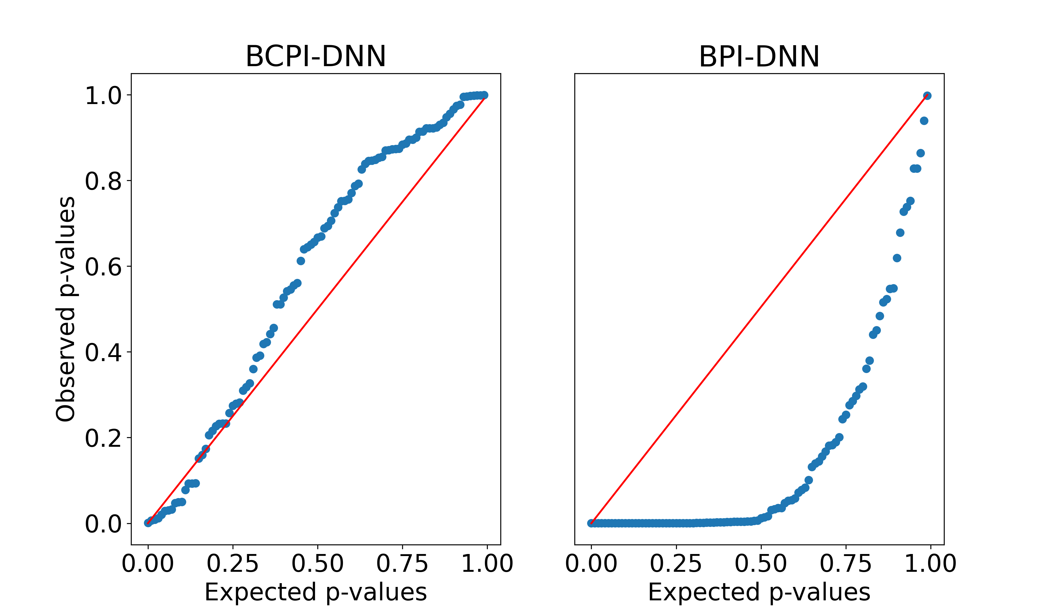
Figure 5: p-values calibration: The calibration of p-values ensuing from BCPI-DNN with the conditional permutation approach is compared to that of BPI-DNN with standard permutation approach. The p-value’s distribution of one randomly selected non significant variable is compared to the uniform distribution. Prediction task was simulated with $n$ = $1000$ and $p$ = $50$.

Appendix F Supplement Figure 1 - Power & Computation time

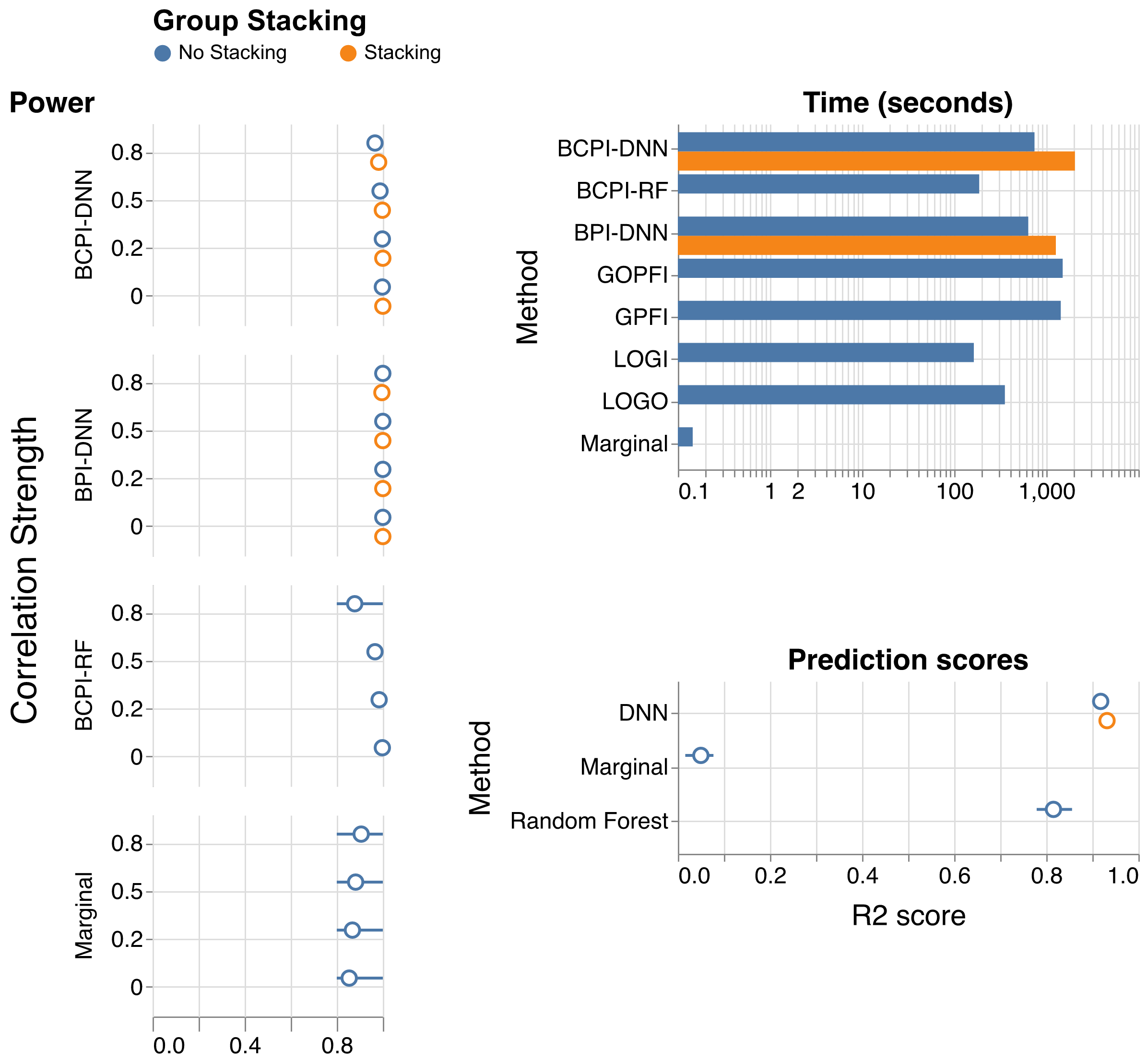
Figure 1 - S1: Benchmarking grouping methods: BCPI-DNN is compared to baseline models and competing approaches for group variable importance providing p-values. (Power) indicates the mean proportion of informative variables identified. (Time) reports the computation time in seconds with $\log_{10}$ scale per core on $100$ cores. (Prediction scores) presents the performance of the different base learners used in the group variable importance methods (Marginal: { Marginal effects}, Random Forest: {BCPI-RF, LOGI, LOGO, GPFI & GOPFI}, DNN: {BPI-DNN & BCPI-DNN}). Prediction tasks were simulated with $n$ = $1000$ and $p$ = $50$.

Appendix G Supplement Figure 1 - AUC score for Grouped Shapley values

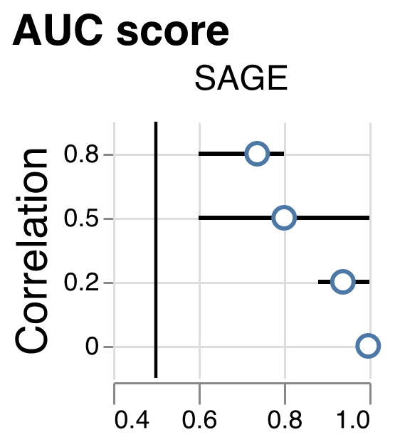
Figure 1 - S2: Grouped Shapley values: Prediction tasks were simulated with $n$ = $1000$ and $p$ = $50$. Solid line: chance level.

The grouped version of SAGE (Global Importance with Shapley values (Covert, Lundberg, and Lee 2020)) was assessed with AUC scores (for detecting important variables) as it does not provide p-values. SAGE performed well in low-correlation settings (mean $\approx 0.95$) but the performance dropped in high-correlation settings (mean $\approx 0.76$).

Appendix H Supplement Figure 1 - AUC score & Type-I error (Non linear case)

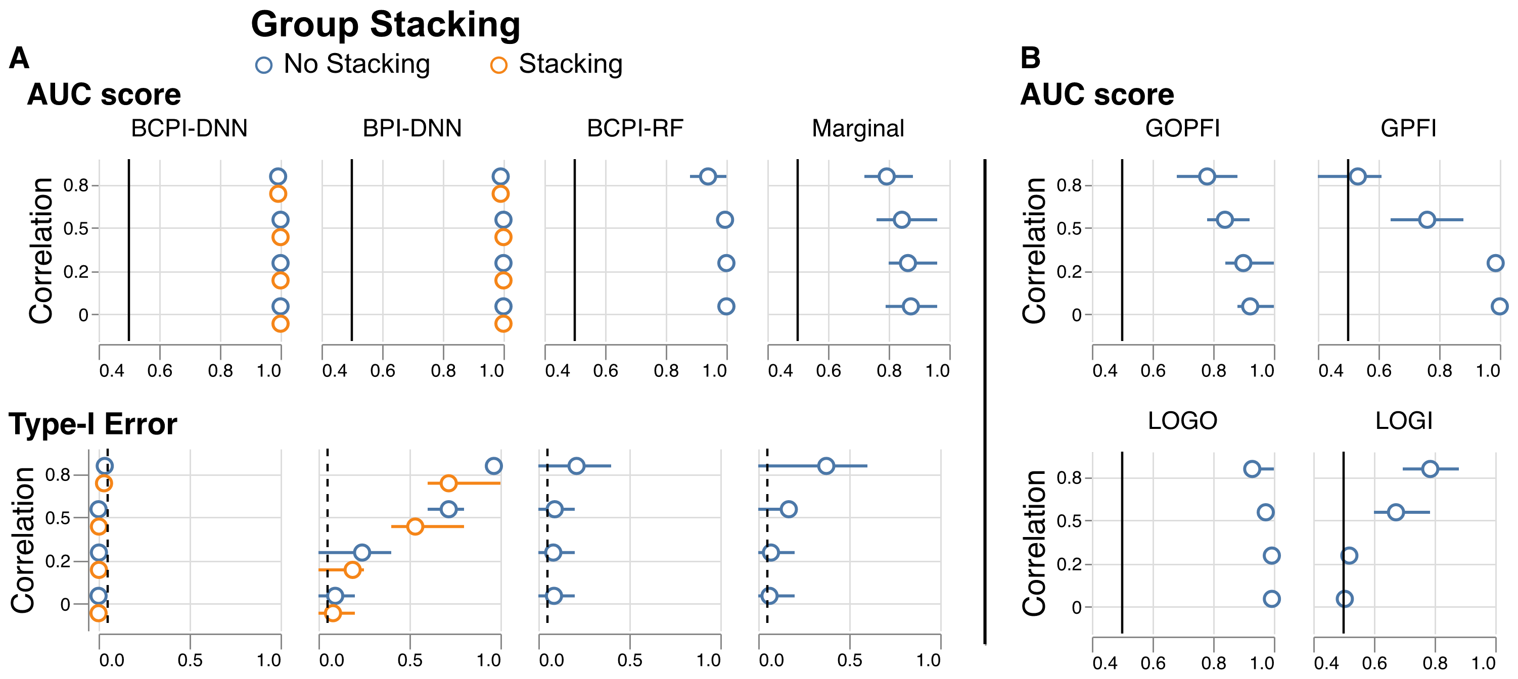
Figure 1 - S3: Benchmarking grouping methods: BCPI-DNN is compared to baseline models and competing approaches for group variable importance. It encompasses two panels: (A) for the methods providing p-values used to check for AUC score and for statistical guarantees (Type-I error control), and (B) for the methods deprived of p-values, thus the importance scores are used to check for AUC score. Prediction tasks were simulated with $n$ = $1000$ and $p$ = $50$. Dashed line: targeted type-I error rate at 5%. Solid line: chance level.

To make the data-generating process more complex, we have added pair interactions to the regression simulation introduced in Fig. 2. The new outcome is set to: $y_{i}=\mathbf{x_{i}}\bm{\beta^{main}}+\text{quad}(\mathbf{x_{i},\beta^{quad}})+\sigma\epsilon_{i},\;\forall i\in\llbracket n\rrbracket$ where the magnitude $\sigma$ of the noise is set to $\frac{||\mathbf{X}\bm{\beta^{\text{main}}}+\text{quad}(\bm{X,\beta^{quad}})||_{2}}{SNR\sqrt{n}}$ and $\textrm{quad}(\bm{x_{i},\beta^{quad}})=\displaystyle\sum_{\underset{k<j}{k,j=1}}^{p_{signals}}\bm{\beta^{quad}}_{k,j}x^{k}_{i}x^{j}_{i}$. The results show that BCPI-DNN outperforms all the alternatives methods presenting high AUC performance coupled with a control for type-I error under the predefined nominal rate. BCPI-RF, where the inference estimator is a Random Forest, showed an almost similar good performance with a little drop in high-correlated settings which can be explained by the drop in the predictive capacity following the plug of the Random Forest.

Appendix I Supplement Figure 1 - Power & Computation time (Non linear case)

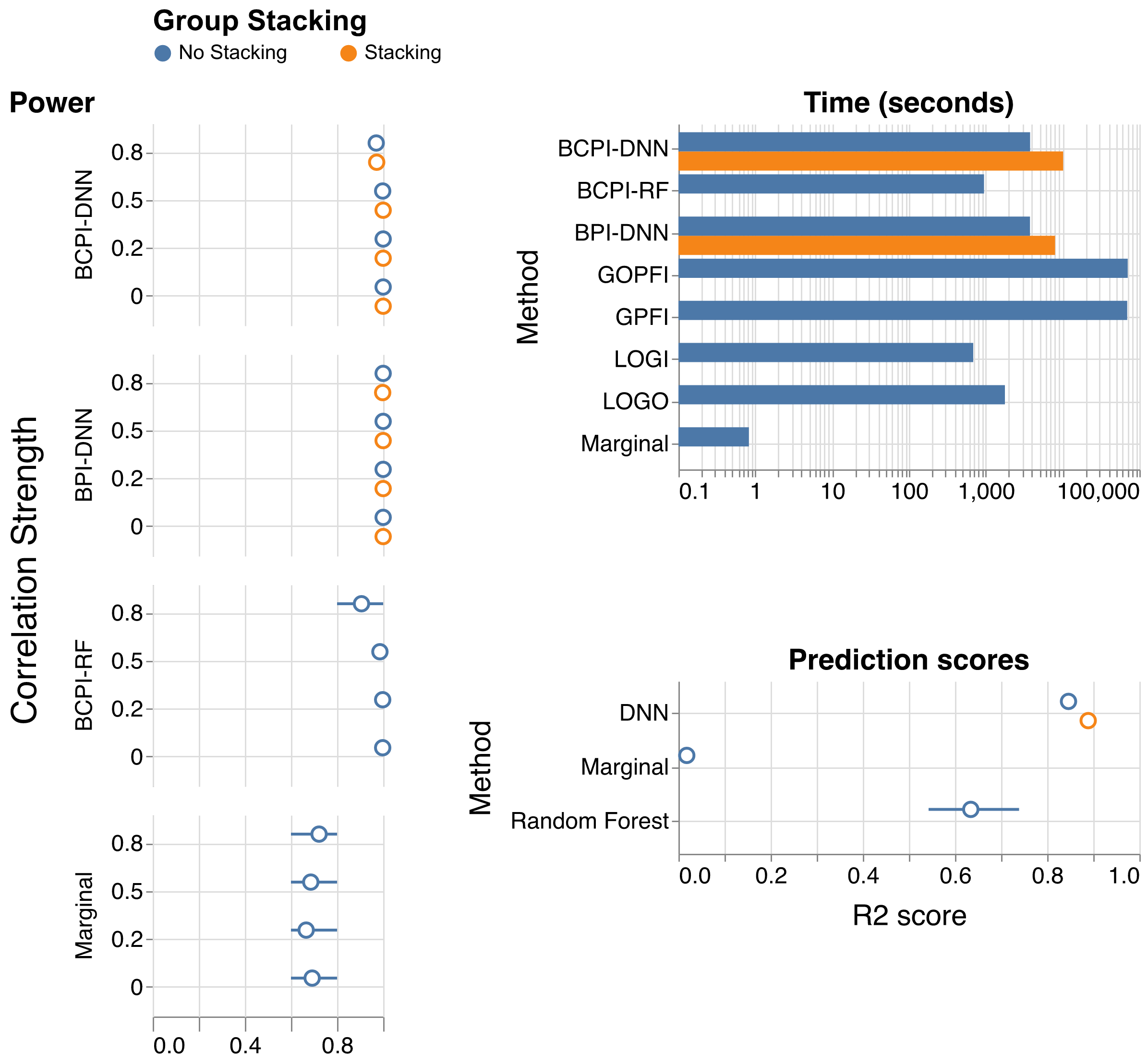
Figure 1 - S4: Benchmarking grouping methods: BCPI-DNN is compared to baseline models and competing approaches for group variable importance providing p-values. (Power) indicates the mean proportion of informative variables identified. (Time) reports the computation time in seconds with $\log_{10}$ scale per core on $100$ cores. (Prediction scores) presents the performance of the different base learners used in the group variable importance methods (Marginal: { Marginal effects}, Random Forest: {BCPI-RF, LOGI, LOGO, GPFI & GOPFI}, DNN: {BPI-DNN & BCPI-DNN}). Prediction tasks were simulated with $n$ = $1000$ and $p$ = $50$.

The results showed that BCPI-DNN, BPI-DNN, BCPI-RF and Marginal attained a high performance.

Appendix J Supplement Figure 2 - Groups with different cardinalities

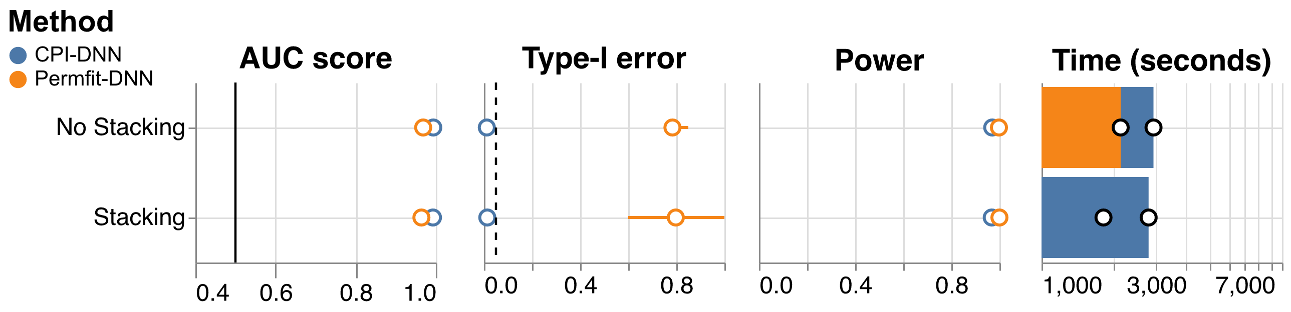
Figure 2 - S1: Groups of different cardinalities: The performance of BCPI-DNN and Permfit-DNN at detecting important groups on simulated data with $n$ = $1000$ and $p$ = $1000$ with $10$ blocks/groups, each group having a cardinality of $10$ with or without the stacking approach. The (AUC score) evaluates the extent to which variables are ranked consistently with the ground truth. The (Type-I error) assesses the rate of low p-values ($\text{p-val}<0.05$). (Power) provides information on the average proportion of detected informative variables ($\text{p-value}<0.05$). The (Time) panel displays computation time in seconds with $\log_{10}$ scale per core on $100$ cores. Dashed line: targeted type-I error rate. Solid line: chance level.

The results showed that BCPI-DNN’s capacity to achieve high AUC performance coupled with a control of Type-I error under the predefined nominal rate was maintained while providing groups of different cardinalities.

References

- Alber et al. (2019) Alber, M.; Buganza Tepole, A.; Cannon, W. R.; De, S.; Dura-Bernal, S.; Garikipati, K.; Karniadakis, G.; Lytton, W. W.; Perdikaris, P.; Petzold, L.; and Kuhl, E. 2019. Integrating Machine Learning and Multiscale Modeling—Perspectives, Challenges, and Opportunities in the Biological, Biomedical, and Behavioral Sciences. npj Digit. Med., 2(1): 1–11.
- Albu, Bocicor, and Czibula (2023) Albu, A.-I.; Bocicor, M.-I.; and Czibula, G. 2023. MM-StackEns: A New Deep Multimodal Stacked Generalization Approach for Protein–Protein Interaction Prediction. Computers in Biology and Medicine, 153: 106526.
- Anatürk et al. (2021) Anatürk, M.; Kaufmann, T.; Cole, J. H.; Suri, S.; Griffanti, L.; Zsoldos, E.; Filippini, N.; Singh-Manoux, A.; Kivimäki, M.; Westlye, L. T.; Ebmeier, K. P.; and de Lange, A.-M. G. 2021. Prediction of Brain Age and Cognitive Age: Quantifying Brain and Cognitive Maintenance in Aging. Hum Brain Mapp, 42(6): 1626–1640.
- Au et al. (2021) Au, Q.; Herbinger, J.; Stachl, C.; Bischl, B.; and Casalicchio, G. 2021. Grouped Feature Importance and Combined Features Effect Plot. arxiv:2104.11688.
- Blesch, Watson, and Wright (2023) Blesch, K.; Watson, D. S.; and Wright, M. N. 2023. Conditional Feature Importance for Mixed Data. AStA Adv Stat Anal.
- Bradley (1997) Bradley, A. P. 1997. The Use of the Area under the ROC Curve in the Evaluation of Machine Learning Algorithms. Pattern Recognition, 30(7): 1145–1159.
- Breiman (2001) Breiman, L. 2001. Random Forests. Machine Learning, 45(1): 5–32.
- Bühlmann (2013) Bühlmann, P. 2013. Statistical Significance in High-Dimensional Linear Models. Bernoulli, 19(4).
- Bycroft et al. (2018) Bycroft, C.; Freeman, C.; Petkova, D.; Band, G.; Elliott, L. T.; Sharp, K.; Motyer, A.; Vukcevic, D.; Delaneau, O.; O’Connell, J.; Cortes, A.; Welsh, S.; Young, A.; Effingham, M.; McVean, G.; Leslie, S.; Allen, N.; Donnelly, P.; and Marchini, J. 2018. The UK Biobank Resource with Deep Phenotyping and Genomic Data. Nature, 562(7726): 203–209.
- Candes et al. (2017) Candes, E.; Fan, Y.; Janson, L.; and Lv, J. 2017. Panning for Gold: Model-X Knockoffs for High-dimensional Controlled Variable Selection. arXiv:1610.02351 [math, stat].
- Chamma, Engemann, and Thirion (2023) Chamma, A.; Engemann, D. A.; and Thirion, B. 2023. Statistically Valid Variable Importance Assessment through Conditional Permutations. arxiv:2309.07593.
- Chen et al. (2016) Chen, G.; Zhang, P.; Li, K.; Wee, C.-Y.; Wu, Y.; Shen, D.; and Yap, P.-T. 2016. Improving Estimation of Fiber Orientations in Diffusion MRI Using Inter-Subject Information Sharing. Sci Rep, 6(1): 37847.
- Chen et al. (2021) Chen, Y.; Wu, X.; Hu, A.; He, G.; and Ju, G. 2021. Social Prediction: A New Research Paradigm Based on Machine Learning. J. Chin. Sociol., 8(1): 15.
- Chevalier et al. (2021) Chevalier, J.-A.; Nguyen, T.-B.; Salmon, J.; Varoquaux, G.; and Thirion, B. 2021. Decoding with Confidence: Statistical Control on Decoder Maps. NeuroImage, 234: 117921.
- Cole and Franke (2017) Cole, J. H.; and Franke, K. 2017. Predicting Age Using Neuroimaging: Innovative Brain Ageing Biomarkers. Trends Neurosci, 40(12): 681–690.
- Constantinescu et al. (2022) Constantinescu, A.-E.; Mitchell, R. E.; Zheng, J.; Bull, C. J.; Timpson, N. J.; Amulic, B.; Vincent, E. E.; and Hughes, D. A. 2022. A Framework for Research into Continental Ancestry Groups of the UK Biobank. Human Genomics, 16(1): 3.
- Covert, Lundberg, and Lee (2020) Covert, I.; Lundberg, S.; and Lee, S.-I. 2020. Understanding Global Feature Contributions With Additive Importance Measures. arxiv:2004.00668.
- Dadi et al. (2021) Dadi, K.; Varoquaux, G.; Houenou, J.; Bzdok, D.; Thirion, B.; and Engemann, D. 2021. Population Modeling with Machine Learning Can Enhance Measures of Mental Health. GigaScience, 10(10): giab071.
- Debeer and Strobl (2020) Debeer, D.; and Strobl, C. 2020. Conditional Permutation Importance Revisited. BMC Bioinformatics, 21(1): 307.
- Engemann et al. (2020) Engemann, D. A.; Kozynets, O.; Sabbagh, D.; Lemaître, G.; Varoquaux, G.; Liem, F.; and Gramfort, A. 2020. Combining Magnetoencephalography with Magnetic Resonance Imaging Enhances Learning of Surrogate-Biomarkers. eLife, 9: e54055.
- Fisher, Rudin, and Dominici (2019) Fisher, A.; Rudin, C.; and Dominici, F. 2019. All Models Are Wrong, but Many Are Useful: Learning a Variable’s Importance by Studying an Entire Class of Prediction Models Simultaneously. arxiv:1801.01489.
- Fleming (2020) Fleming, G. 2020. How and Why to Interpret Black Box Models.
- Gao et al. (2022) Gao, Y.; Stevens, A.; Willet, R.; and Raskutti, G. 2022. Lazy Estimation of Variable Importance for Large Neural Networks. arxiv:2207.09097.
- Gregorutti, Michel, and Saint-Pierre (2015) Gregorutti, B.; Michel, B.; and Saint-Pierre, P. 2015. Grouped Variable Importance with Random Forests and Application to Multiple Functional Data Analysis. Computational Statistics & Data Analysis, 90: 15–35.
- Hooker, Mentch, and Zhou (2021) Hooker, G.; Mentch, L.; and Zhou, S. 2021. Unrestricted Permutation Forces Extrapolation: Variable Importance Requires at Least One More Model, or There Is No Free Variable Importance. arxiv:1905.03151.
- Hooker et al. (2019) Hooker, S.; Erhan, D.; Kindermans, P.-J.; and Kim, B. 2019. A Benchmark for Interpretability Methods in Deep Neural Networks. arxiv:1806.10758.
- Janitza, Celik, and Boulesteix (2018) Janitza, S.; Celik, E.; and Boulesteix, A.-L. 2018. A Computationally Fast Variable Importance Test for Random Forests for High-Dimensional Data. Adv Data Anal Classif, 12(4): 885–915.
- Jonsson et al. (2019) Jonsson, B. A.; Bjornsdottir, G.; Thorgeirsson, T. E.; Ellingsen, L. M.; Walters, G. B.; Gudbjartsson, D. F.; Stefansson, H.; Stefansson, K.; and Ulfarsson, M. O. 2019. Brain Age Prediction Using Deep Learning Uncovers Associated Sequence Variants. Nat Commun, 10(1): 5409.
- Knutson and Pan (2020) Knutson, K. A.; and Pan, W. 2020. Integrating Brain Imaging Endophenotypes with GWAS for Alzheimer’s Disease. Quant Biol.
- Kora et al. (2021) Kora, P.; Meenakshi, K.; Swaraja, K.; Rajani, A.; and Raju, M. S. 2021. EEG Based Interpretation of Human Brain Activity during Yoga and Meditation Using Machine Learning: A Systematic Review. Complementary Therapies in Clinical Practice, 43: 101329.
- Lee, Sood, and Craven (2018) Lee, K.; Sood, A.; and Craven, M. 2018. Understanding Learned Models by Identifying Important Features at the Right Resolution. arxiv:1811.07279.
- Lei et al. (2018) Lei, J.; G’Sell, M.; Rinaldo, A.; Tibshirani, R. J.; and Wasserman, L. 2018. Distribution-Free Predictive Inference for Regression. Journal of the American Statistical Association, 113(523): 1094–1111.
- Littlejohns et al. (2020) Littlejohns, T. J.; Holliday, J.; Gibson, L. M.; Garratt, S.; Oesingmann, N.; Alfaro-Almagro, F.; Bell, J. D.; Boultwood, C.; Collins, R.; Conroy, M. C.; Crabtree, N.; Doherty, N.; Frangi, A. F.; Harvey, N. C.; Leeson, P.; Miller, K. L.; Neubauer, S.; Petersen, S. E.; Sellors, J.; Sheard, S.; Smith, S. M.; Sudlow, C. L. M.; Matthews, P. M.; and Allen, N. E. 2020. The UK Biobank Imaging Enhancement of 100,000 Participants: Rationale, Data Collection, Management and Future Directions. Nat Commun, 11(1): 2624.
- Louppe et al. (2013) Louppe, G.; Wehenkel, L.; Sutera, A.; and Geurts, P. 2013. Understanding Variable Importances in Forests of Randomized Trees. In Advances in Neural Information Processing Systems, volume 26. Curran Associates, Inc.
- Lundberg, Brand, and Jeon (2022) Lundberg, I.; Brand, J. E.; and Jeon, N. 2022. Researcher Reasoning Meets Computational Capacity: Machine Learning for Social Science. Social Science Research, 108: 102807.
- Mi et al. (2021) Mi, X.; Zou, B.; Zou, F.; and Hu, J. 2021. Permutation-Based Identification of Important Biomarkers for Complex Diseases via Machine Learning Models. Nat Commun, 12(1): 3008.
- Molnar (2022) Molnar, C. 2022. Interpretable Machine Learning.
- Molnar et al. (2021a) Molnar, C.; König, G.; Bischl, B.; and Casalicchio, G. 2021a. Model-Agnostic Feature Importance and Effects with Dependent Features – A Conditional Subgroup Approach. arxiv:2006.04628.
- Molnar et al. (2021b) Molnar, C.; König, G.; Herbinger, J.; Freiesleben, T.; Dandl, S.; Scholbeck, C. A.; Casalicchio, G.; Grosse-Wentrup, M.; and Bischl, B. 2021b. General Pitfalls of Model-Agnostic Interpretation Methods for Machine Learning Models. arxiv:2007.04131.
- Mutz and Lewis (2021) Mutz, J.; and Lewis, C. M. 2021. Lifetime Depression and Age-Related Changes in Body Composition, Cardiovascular Function, Grip Strength and Lung Function: Sex-Specific Analyses in the UK Biobank. Aging (Albany NY), 13(13): 17038–17079.
- Newby et al. (2021) Newby, D.; Winchester, L.; Sproviero, W.; Fernandes, M.; Wang, D.; Kormilitzin, A.; Launer, L. J.; and Nevado-Holgado, A. J. 2021. Associations Between Brain Volumes and Cognitive Tests with Hypertensive Burden in UK Biobank. J Alzheimers Dis, 84(3): 1373–1389.
- Pedregosa et al. (2011) Pedregosa, F.; Varoquaux, G.; Gramfort, A.; Michel, V.; Thirion, B.; Grisel, O.; Blondel, M.; Prettenhofer, P.; Weiss, R.; Dubourg, V.; Vanderplas, J.; Passos, A.; Cournapeau, D.; Brucher, M.; Perrot, M.; and Duchesnay, É. 2011. Scikit-Learn: Machine Learning in Python. Journal of Machine Learning Research, 12(85): 2825–2830.
- Popescu et al. (2021) Popescu, S. G.; Glocker, B.; Sharp, D. J.; and Cole, J. H. 2021. Local Brain-Age: A U-Net Model. Front Aging Neurosci, 13: 761954.
- Rahim et al. (2015) Rahim, M.; Thirion, B.; Abraham, A.; Eickenberg, M.; Dohmatob, E.; Comtat, C.; and Varoquaux, G. 2015. Integrating Multimodal Priors in Predictive Models for the Functional Characterization of Alzheimer’s Disease. In Navab, N.; Hornegger, J.; Wells, W. M.; and Frangi, A., eds., Medical Image Computing and Computer-Assisted Intervention – MICCAI 2015, Lecture Notes in Computer Science, 207–214. Cham: Springer International Publishing. ISBN 978-3-319-24553-9.
- Ribeiro, Singh, and Guestrin (2016) Ribeiro, M. T.; Singh, S.; and Guestrin, C. 2016. ”Why Should I Trust You?”: Explaining the Predictions of Any Classifier. arxiv:1602.04938.
- Roibu et al. (2023) Roibu, A.-C.; Adaszewski, S.; Schindler, T.; Smith, S. M.; Namburete, A. I.; and Lange, F. J. 2023. Brain Ages Derived from Different MRI Modalities Are Associated with Distinct Biological Phenotypes. In 2023 10th IEEE Swiss Conference on Data Science (SDS), 17–25.
- Sabbagh et al. (2023) Sabbagh, D.; Cartailler, J.; Touchard, C.; Joachim, J.; Mebazaa, A.; Vallée, F.; Gayat, É.; Gramfort, A.; and Engemann, D. A. 2023. Repurposing Electroencephalogram Monitoring of General Anaesthesia for Building Biomarkers of Brain Ageing: An Exploratory Study. BJA Open, 7.
- Strobl et al. (2008) Strobl, C.; Boulesteix, A.-L.; Kneib, T.; Augustin, T.; and Zeileis, A. 2008. Conditional Variable Importance for Random Forests. BMC Bioinformatics, 9(1): 307.
- Strzelecki and Badura (2022) Strzelecki, M.; and Badura, P. 2022. Machine Learning for Biomedical Application. Applied Sciences, 12(4): 2022.
- Sudlow et al. (2015) Sudlow, C.; Gallacher, J.; Allen, N.; Beral, V.; Burton, P.; Danesh, J.; Downey, P.; Elliott, P.; Green, J.; Landray, M.; Liu, B.; Matthews, P.; Ong, G.; Pell, J.; Silman, A.; Young, A.; Sprosen, T.; Peakman, T.; and Collins, R. 2015. UK Biobank: An Open Access Resource for Identifying the Causes of a Wide Range of Complex Diseases of Middle and Old Age. PLOS Medicine, 12(3): e1001779.
- Tae et al. (2018) Tae, W.-S.; Ham, B.-J.; Pyun, S.-B.; Kang, S.-H.; and Kim, B.-J. 2018. Current Clinical Applications of Diffusion-Tensor Imaging in Neurological Disorders. J Clin Neurol, 14(2): 129–140.
- Valentin, Harkotte, and Popov (2020) Valentin, S.; Harkotte, M.; and Popov, T. 2020. Interpreting Neural Decoding Models Using Grouped Model Reliance. PLoS Computational Biology, 16(1).
- Watson and Wright (2021) Watson, D. S.; and Wright, M. N. 2021. Testing Conditional Independence in Supervised Learning Algorithms. Mach Learn, 110(8): 2107–2129.
- Wehenkel et al. (2018) Wehenkel, M.; Sutera, A.; Bastin, C.; Geurts, P.; and Phillips, C. 2018. Random Forests Based Group Importance Scores and Their Statistical Interpretation: Application for Alzheimer’s Disease. Frontiers in Neuroscience, 12.
- Williamson et al. (2021) Williamson, B. D.; Gilbert, P. B.; Simon, N. R.; and Carone, M. 2021. A General Framework for Inference on Algorithm-Agnostic Variable Importance. Journal of the American Statistical Association, 0(0): 1–14.
- Wolpert (1992) Wolpert, D. H. 1992. Stacked Generalization. Neural Networks, 5(2): 241–259.
- Zhou et al. (2021) Zhou, Q.; Liang, H.; Lin, Z.; and Xu, K. 2021. Multimodal Feature Fusion for Video Advertisements Tagging Via Stacking Ensemble. arxiv:2108.00679.