Prediction of the bubble wall velocity for a large jump in degrees of freedom

Abstract

The bubble expansion velocity is an important parameter in the prediction of gravitational waves from first order phase transitions. This parameter is difficult to compute, especially in phase transitions in strongly coupled theories. In this work, we present a method to estimate the wall velocity for phase transitions with a large enthalpy jump, valid for weakly and strongly coupled theories. We find that detonations are disfavored in this limit, but wall velocities are not necessarily small. We also investigate the effect of two other features in the equation of state: non-conformal sound speeds and a limited range of temperatures for which the phases exist. We find that the former can increase the wall velocity for a given nucleation temperature, and the latter can restrict the wall velocities to small values. To test our approach, we use holographic phase transitions, which typically display these three features. We find excellent agreement with numerically obtained values of the wall velocity. We also demonstrate that the implications for gravitational waves can be significant.

I Introduction

Many models for particle physics beyond the Standard Model (BSM) predict that one or more first order phase transitions (PTs) might have occurred in the history of the universe. Such PTs can source a gravitational wave (GW) signal when the released vacuum energy gets converted into sound waves, gradient energy in the bubble walls and/or turbulence Witten:1984rs ; Kosowsky:1991ua ; Kosowsky:1992rz ; Kamionkowski:1993fg . Depending on the strength and temperature of these transitions, the signals could be observable with the next generation of GW telescopes Grojean:2006bp ; Caprini:2018mtu ; Caprini:2019egz .

Using GWs to learn about BSM physics requires accurate predictions of the GW spectrum. Analytical arguments and hydrodynamic simulations have resulted in a predicted GW spectrum as a broken power-law Hindmarsh:2015qta ; Hindmarsh:2017gnf ; Caprini:2019egz ; Hindmarsh:2016lnk ; Hindmarsh:2019phv ; Jinno:2020eqg ; Jinno:2022mie ; RoperPol:2023dzg . The underlying assumption in Caprini:2019egz ; Hindmarsh:2016lnk ; Hindmarsh:2019phv ; Jinno:2020eqg ; Jinno:2022mie ; RoperPol:2023dzg , which was checked in Hindmarsh:2015qta ; Hindmarsh:2017gnf , is that the amplitude of the signal can be predicted by the nucleation temperature $T_{n}$ and rate $\beta$, wall velocity $\xi_{w}$ and sound speed $c_{s}$, as well as the so-called energy budget, that can be computed from the hydrodynamics of a single bubble. In most cases, the energy budget can be estimated from the phase transition strength $\alpha$, $\xi_{w}$ Espinosa:2010hh , and $c_{s}$ Giese:2020rtr ; Giese:2020znk . The challenge of predicting the GW spectrum is thus reduced to a computation of the thermal parameters and the hydrodynamics.

The wall velocity strongly affects the strength and shape of the GW spectrum Espinosa:2010hh ; Caprini:2019egz , but is challenging to compute for a given theory (see however Moore:1995si ; Dorsch:2018pat ; Lewicki:2021pgr ; Laurent:2022jrs ; Jiang:2022btc for some explicit computations) and is therefore often treated as a free parameter, or simply set to $\xi_{w}\to 1$. This results in a significant uncertainty, so better estimates are necessary. Unfortunately, the difficulty of computing the wall velocity is even greater in strongly coupled theories Schwaller:2015tja ; Bruggisser:2018mrt ; Huang:2020crf ; Halverson:2020xpg ; Yang:2022ghc , where a quasiparticle interpretation underlying the computations of Moore:1995si ; Dorsch:2018pat ; Lewicki:2021pgr ; Laurent:2022jrs ; Jiang:2022btc may not be available. In this work, we will provide a way to determine $\xi_{w}$ that can be applied to both weakly and strongly coupled theories when they have a large jump in the number of degrees of freedom between the phases – we will refer to this as a large enthalpy jump. We will take a holographic equation of state (EoS) as an explicit example, which can be used to understand aspects of strongly coupled PTs Nitti:2008za ; Nitti:2009jd . Holographic models represent a useful playground where we can obtain insight into strongly coupled cosmological PTs Bigazzi:2020phm ; Ares:2020lbt ; Bigazzi:2020avc ; Ares:2021ntv ; Zhu:2021vkj ; Morgante:2022zvc ; Chen:2022cgj and possibly into PTs in neutron star mergers Casalderrey-Solana:2022rrn . It has already been shown that $\xi_{w}$ can be obtained in a holographic PT Bea:2021 ; Bea:2022 ; Bigazzi:2021ucw ; Janik:2022wsx , and we can use these results to test our approach.

Holographic theories are characterized by a gravitational description that is dual to a strongly coupled gauge theory with a large number $N$ of degrees of freedom. They naturally exhibit three distinctive features (see e.g. Bea:2018whf ; Elander:2020rgv ):

• A large jump in enthalpy between the high-temperature and low-temperature phase,

• A limited range of temperature for which the phases exist,

• Strong deviation in the sound speed from the conformal value $c_{s}^{2}=1/3$.

We will see that these features can strongly modify the hydrodynamic predictions compared to the often-made assumptions that $c_{s}^{2}\sim 1/3$ and that the temperature can take any value. We also stress that these features are not unique to holographic PTs, and that our results apply to non-holographic models as well.

The main result of this work is a demonstration that the wall velocity for models with a large enthalpy jump follows directly from the EoS and the nucleation temperature, without further details of the plasma. Some steps in this direction were already taken in Janik:2022wsx , where a formula was proposed to obtain the wall speed for planar bubbles. Our results are valid for spherical bubbles and we will compare our results for planar bubbles with the findings there. Additionally, detonations are not realizable in the infinite enthalpy jump limit. If the allowed temperature range is limited, we find that the resulting wall velocity is rather small, favoring deflagrations as observed in Bea:2021 ; Bea:2022 ; Janik:2022wsx , and likely excluding detonations. Finally, we will see that quantitative results can get strongly affected by a non-conformal sound speed. GW predictions for models with a large enthalpy jump get significant corrections compared to the ‘vanilla’ assumption where $\xi_{w}$ is a free parameter and $c_{s}^{2}=1/3$.

II Hydrodynamic and thermodynamic description of bubble expansion

II.1 Hydrodynamics

Finding the kinetic energy in the fluid requires solving the hydrodynamic equations of a single expanding bubble. We will summarize the approach here, and further details can be found in landau1987fluid ; Kurki-Suonio:1995rrv ; Kamionkowski:1993fg ; Espinosa:2010hh . The hydrodynamic equations follow from the energy-momentum tensor of a perfect fluid,

$$T^{\mu\nu}=wu^{\mu}u^{\nu}-pg^{\mu\nu},$$ (1)

where $w=Tdp/dT$ is the enthalpy. $g^{\mu\nu}$ denotes the metric, which is assumed to be the Minkowski metric, and $u^{\mu}=\gamma(1,\vec{v})$ denotes the fluid velocity with $\gamma=1/\sqrt{1-\vec{v}^{2}}$. The hydrodynamic equations for $u^{\mu}$ and $w$ are obtained by projecting $\partial_{\mu}T^{\mu\nu}=0$ in the direction parallel and perpendicular to the fluid flow:

$$2\frac{v}{\xi} =\gamma^{2}(1-v\xi)\left[\frac{\mu^{2}(\xi,v)}{c_{s}^{2}}-1\right]\partial_{\xi}v,$$ (2)

$$\partial_{\xi}w =w\left(1+\frac{1}{c_{s}^{2}}\right)\gamma^{2}\mu(\xi,v)\partial_{\xi}v,$$

where $\xi=r/t$ (with $r$ the radial distance to the center of the bubble and $t$ the time since nucleation), $v$ the fluid velocity in radial coordinates and $\mu$ is the Lorentz-boosted velocity, $\mu(\xi,v)=(\xi-v)/(1-\xi v)$. The speed of sound follows from $p$ via

$$c_{s}^{2}=\frac{dp/dT}{de/dT},\qquad e=p\frac{dp}{dT}-p.$$ (3)

The only regions where this hydrodynamic description fails are the bubble walls and shocks. Nevertheless, given their small size compared to the bubble, they can be replaced by discontinuities across which we impose matching conditions, that are obtained by integration $\partial_{\mu}T^{\mu\nu}=0$ from right behind the wall/shock to right in front of the wall/shock, yielding

$$w_{+}v_{+}^{2}\gamma_{+}^{2}+p_{+}=w_{-}v_{-}^{2}\gamma_{-}^{2},\qquad w_{+}v_{+}\gamma_{+}^{2}=w_{-}v_{-}\gamma_{-}^{2},$$ (4)

where the $+,(-)$ label denotes quantities evaluated right in front of (behind) the discontinuity. After some algebraic manipulations, we obtain

$$v_{+}v_{-}=\frac{p_{+}-p_{-}}{e_{+}-e_{-}}\quad\quad\frac{v_{+}}{v_{-}}=\frac{e_{-}+p_{+}}{e_{+}+p_{-}},$$ (5)

for the matching conditions. Note that the velocities are defined with respect to the frame of the wall/shock.

By solving eqs. (2) and imposing the matching conditions eqs. (5) at the wall and possible shock we can solve for the whole flow as a function of two input parameters, e.g. $\xi_{w}$ and $T_{n}$ (or, similarly, $\alpha_{n}$). The energy budget $K$ is determined from the ratio of the fluid kinetic energy to the enthalpy of the high-temperature phase at $T_{n}$. For each $T_{n}$, there are three type of solutions depending on the value of the wall speed with respect to the sound speed (see, e.g. Espinosa:2010hh ):

• Deflagrations: $\xi_{w}<c_{s,L}$. In this case $v_{-}=\xi_{w}$ and $v_{+}<c_{s,H}(T_{+})$.

• Hybrids: $c_{s,L}<\xi_{w}<v_{J}$, with $v_{J}$ the Jouguet velocity (see e.g. Kurki-Suonio:1995rrv ; Espinosa:2010hh ; Ai:2023see ). We now have $v_{-}=c_{s,L}$ and $v_{+}<=c_{s,H}$.

• Detonations: $\xi_{w}>v_{J}$, with $v_{-}>c_{s,L}$ and $v_{+}=\xi_{w}$.

Here and in the following we use the subscript $H$ ($L$) for quantities defined in the high- (low-) enthalpy phase.

II.2 Equations of state

Figure 1: Speed of sound squared and pressure (inset) of the high enthalpy phase. The dashed lines correspond to states that are thermodynamically unstable.

We will consider three equations of state to investigate the effects of large enthalpy jumps, temperature limitations and $c_{s}^{2}\neq 1/3$ on the hydrodynamic solutions. Let us parametrize the large enthalpy jump by some large number $N$, and assume that low-enthalpy phase quantities are suppressed by $1/N^{2}$.

Dark SU(N) model

We consider the model of Nitti:2008za ; Nitti:2009jd , which is based on a holographic description of a confinement/deconfinement PT. The thermodynamic equation of state can be obtained following the approach described in Nitti:2008za , which we will not repeat here, but we demonstrate the pressure and sound speed of the high-enthalpy phase in fig. 1. We see that the sound speed deviates strongly from $c_{s}^{2}=1/3$. At the nucleation temperature $T_{n}=0.993T_{c}$ Morgante:2022zvc , $c_{s}^{2}=0.103$. Note that the model only describes the high-enthalpy phase, which ceases to exist at $T<T_{\rm min,SU(N)}$. Even though we leave $N$ as a free parameter, the model implicitly assumes that $N$ is large, as contributions that are smaller than $\mathcal{O}(N^{2})$ are neglected. For the low-enthalpy phase, we will assume the equation of state proposed by Leitao:2014pda (although we will find that nothing depends on this for large $N$)

$$p_{L}=\frac{1}{N^{2}}\frac{T_{c}^{4}}{\nu-1}\left(\frac{T}{T_{c}}\right)^{\nu},$$ (6)

where the sound speed is a constant set by $\nu=1+1/c_{s,L}^{2}$, which parameterizes the unknown equation of state of the low-enthalpy phase.

Template model

We use the model of Leitao:2014pda to describe models with constant, but non-conformal sound speeds,

$$p_{H}=\frac{a_{H}T_{c}^{4}}{\mu-1}\left(\frac{T}{T_{c}}\right)^{\mu}-\epsilon,\qquad p_{L}=\frac{1}{N^{2}}\frac{a_{H}T_{c}^{4}}{\nu-1}\left(\frac{T}{T_{c}}\right)^{\nu},$$ (7)

where and $\mu=1+1/c_{s,H}^{2}$ and $a_{H}$ parameterizes the number of degrees of freedom of the high-enthalpy phase and $\epsilon$ is a temperature-independent constant, which parameterizes the energy difference between the two phases. The virtue of the template model is that it allows us to study the effect of the non-conformal sound speed and large enthalpy jump, without the limited temperature range. The often-used bag equation of state is a special case of the template model with $\mu=\nu=4$.

In all cases, we assume that the low-enthalpy phase temperature cannot grow as large as to undo the $1/N^{2}$ suppression, i.e. we assume that $T_{L}\ll T_{c}N^{2/\nu}$.

Strongly coupled holographic model

We will briefly discuss the model of Bea:2022 in sec. III.3, a holographic description of a strongly coupled phase transition with $N\sim 3$. (see Bea:2022 for details). The bubble wall velocity of this model was determined in Bea:2021 , and we will compare it to our estimate.

III Hydrodynamics with a large enthalpy jump

III.1 Matching conditions

Let us consider the matching conditions of eq.(5) in the limit of large $N$. Given the suppression that we assumed for the low-enthalpy phase, the following ratios hold,

$$\frac{w_{-}}{w_{+}}\sim\frac{s_{-}}{s_{+}}\sim\frac{e_{-}}{e_{+}}\sim\frac{1}{N^{2}},$$ (8)

where $s=w/T$. We have assumed the previously mentioned bound on the low-enthalpy phase temperature.

The relation between the pressures of both phases is more complicated. By the definition of $T_{c}$, $p_{H}(T_{c})=p_{L}(T_{c})$, which means that $p_{-}/p_{+}$ does not need to be small. Indeed,

$$\frac{p_{-}}{p_{+}}\sim\frac{1}{N^{2}} \mathrm{if}\quad\frac{|T_{+}-T_{c}|}{T_{c}}\gg\frac{1}{N^{2}},\qquad\textbf{Case 1,}$$ (9)

$$\frac{p_{-}}{p_{+}}\sim 1 \mathrm{if}\quad\frac{|T_{+}-T_{c}|}{T_{c}}\lesssim\frac{1}{N^{2}},\qquad\textbf{Case 2.}$$

We will now study the matching conditions for these two different cases.

Case 1

Let us first investigate eq. (5) with $p_{-}/p_{+}\sim 1/N^{2}$,

$$v_{+}v_{-}\sim\frac{p_{+}}{e_{+}}\left(1+\mathcal{O}\left(\frac{1}{N^{2}}\right)\right)\sim\frac{v_{+}}{v_{-}},$$ (10)

with solution $v_{-}=1-\mathcal{O}(1/N^{2})$, which corresponds to a detonation, as we have seen in sec. II.1. In a detonation, $v_{+}>v_{-}$, so eq. (4) implies that $w_{-}>w_{+}$, which is not possible in the large $N$ limit.

Case 2

If, $p_{-}/p_{+}\sim 1$, then,

$$v_{+}v_{-}=\mathcal{O}\left(\frac{1}{N^{2}}\right),\qquad\frac{v_{+}}{v_{-}}=\mathcal{O}\left(\frac{1}{N^{2}}\right),$$ (11)

implying that $v_{+}=\mathcal{O}(1/N^{2})$, corresponding to a deflagration or a hybrid. In combination with eq. (9) this leads to the following conditions for a large enthalpy jump bubble expansion,

$$T_{+}=T_{c}\quad\mathrm{and}\quad v_{+}=0.$$ (12)

The condition on $v_{+}$ was already stated in Janik:2022wsx while the one for $T_{+}$ was remarked there as a good approximation for the simulations presented in Bea:2021 ; Janik:2022wsx .

Let us point out that the matching relation just obtained does not restrict us to slow walls, as the Jouguet velocity, which is the transition from hybrids to detonations can become arbitrarily close to unity for a large amount of supercooling (see e.g. Espinosa:2010hh ).

We conclude that large enthalpy jump PTs lead to deflagrations or hybrids characterized by the condition (12) while detonations are excluded.

III.2 Hydrodynamic solutions

We expect the matching relations of eq. (12) to hold in any theory with a large enthalpy jump, but in order to use them to find the relation between $\xi_{w}$ and $T_{n}$ requires a solution of the hydrodynamic equations in the shock wave. This requires an EoS, and the relation between $\xi_{w}$ and $T_{n}$ will be numerical.

In this section, we solve the hydrodynamics for the dark SU(N) and the template model (with $c_{s}^{2}=1/3$ and $c_{s}^{2}=0.103$ – the same value as in the dark SU(N)), for increasing $N$.

Let us focus first on deflagrations and hybrids. We demonstrate in the top panel of fig. 2 that $T_{+}$ indeed approaches $T_{c}$, independent of the choice of $T_{-}$. The slower converge for larger $T_{-}$ is to be expected as we require larger $N$ to suppress the enthalpy at higher temperatures. We used the template model with $\mu,\nu=4$, but have confirmed explicitly that the convergence also occurs for other sound speeds and the dark SU(N) model. We have furthermore verified explicitly that $v_{+}$ approaches zero.

Figure 2: Top: $T_{+}/T_{c}$ as a function of $N$ for different choices of $T_{-}$. Bottom: Wall speed as a function of the nucleation temperature in the dark SU(N) model (black), template model with $c_{s}^{2}=1/3$ (pink dot-dashed) and with $c_{s}^{2}=0.103$ (cyan dashed). Circles correspond to deflagrations and triangles to hybrids.

The lines in the bottom panel of fig. 2 demonstrate the relation $\xi_{w}(T_{n})$ obtained from solving the hydrodynamic equations with the matching conditions of eq. (12). In this limit, the solution is obtained without any reference to the fluid behind the wall. The dots demonstrate the result for $N=30$ (with $\nu=4$ and $T_{-}/T_{c}=1.2$) and we see that they agree extremely well. We observe that for the holographic model, only solutions with $\xi_{w}\lesssim 0.25$ exist. The reason becomes immediately clear – the minimum temperature of the high-enthalpy phase prevents further supercooling. From the results of the template model, we see that when such a minimum temperature does not exist, there is – in principle – no limit on the amount of supercooling and the wall velocity can grow arbitrarily large. This is a very important observation, as it suggests that the low wall velocities found in real-time holographic simulations Janik:2022wsx ; Bea:2021 ; Bea:2022 are not a result of the strongly coupled nature of these theories, but rather of the impossibility of strong supercooling.

Another interesting observation is that the sound speed strongly affects the relation between $T_{n}$ and $\xi_{w}$. For models with $c_{s}^{2}<1/3$, the typical velocity is larger than for $c_{s}^{2}=1/3$, and a smaller amount of supercooling is required for a fast wall, in agreement with Janik:2022wsx .

Finally, we checked that detonations get excluded in the large enthalpy jump limit for the template model. Given a fixed $\xi_{w}$ and $T_{n}$, eq. (5) implies that $p_{-}$ and $e_{-}$ are independent of $N$, meaning that the temperature scales as $T_{-}\propto T_{c}N^{2/\nu}$ for detonations. But this corresponds precisely to the range of temperatures that we excluded in the large $N$ limit because it undoes the $1/N^{2}$ suppression.

III.3 Comparison with the strongly coupled holographic model

Figure 3: Wall speed from the simulations in (Bea:2021, ) (dots), and the result using the condition (12) (solid black), local thermal equilibrium (dashed cyan) and the simple wave formula (14)

(dot-dashed pink).

Let us now put our result to the test, by comparing to the wall velocity obtained in an actual simulation. Fig. 3 demonstrates a comparison to the values of $\xi_{w}$ obtained in the strongly coupled holographic model in Bea:2021 for planar bubbles. In this case, $\partial_{\mu}T^{\mu\nu}=0$ reduces to $\partial_{\xi}v=\partial_{\xi}w=0$ for deflagrations and one only has to solve the matching conditions at the shock.

We see that the large enthalpy jump description (solid black) already gives a very accurate estimate of the wall velocity, even though $N$ is only approximately 3. We also compare the result to the wall velocity obtained assuming local thermal equilibrium at the bubble wall (dashed cyan) BarrosoMancha:2020fay ; Ai:2021kak ; Ai:2023see and interestingly this gives a comparable estimate, albeit somewhat larger. This can be understood in the large enthalpy jump limit as follows. The entropy change at the wall, in the wall frame, is given by

$$s_{H}(T_{+})\gamma_{+}v_{+}-s_{L}(T_{-})\gamma_{-}v_{-}=0,$$ (13)

which vanishes due to $v_{+}=0$ and $s_{-}=0$ when $N\rightarrow\infty$. This is exactly the condition for local thermal equilibrium and we would therefore expect an even better agreement between the two approaches for larger $N$.

Additionally, we display the prediction of the simple wave (sw) formula (Janik:2022wsx, ) (pink dot-dashed), with the additional assumption $v_{+}=0$ and $T_{+}=T_{c}$,

$$\xi_{w}=\tanh\int_{T_{n}}^{T_{c}}\frac{dT}{Tc_{s}}.$$ (14)

Notice that the results are very close to ours for $T_{n}\sim T_{c}$, but start disagreeing for smaller $T_{n}$. This effect can be perfectly understood in the template model, where both approaches offer analytical results,

$$\xi_{w}^{{\rm large\,}N} =\frac{c_{s,H}(T_{c}^{\mu}-T_{n}^{\mu})}{\sqrt{(T_{c}^{\mu}+c_{s,H}^{2}T_{n}^{\mu})(T_{n}^{\mu}+c_{s,H}^{2}T_{c}^{\mu})}},$$ (15)

$$\xi_{w}^{\rm sw} =\tanh\left(\frac{1}{c_{s,H}}\log\frac{T_{c}}{T_{n}}\right),$$

with $\mu=1+1/c_{s,H}^{2}$. The series expansions of both expressions around $T_{n}=T_{c}$ agree perfectly to second order. However, greater discrepancy with the data is expected for theories with stronger supercooling.

IV Implications for GWs

Let us now discuss the possible implications for the GW spectrum, taking the dark SU(N) model and the template model as concrete examples. For the prediction of the GW spectrum, we follow Caprini:2019egz .

In Morgante:2022zvc , the GW spectrum of the dark SU(N) model was predicted for three different values of the wall velocity $\xi_{w}=(0.01,0.1,1)$, for a nucleation temperature of $T_{n}/T_{c}\sim 0.993$. Using the given nucleation temperature, we find that the correct wall velocity is $\xi_{w}=0.078$ in the large enthalpy limit (which is implicitly used in Morgante:2022zvc , by assuming that the low-enthalpy phase can be ignored). The sound speed deviates strongly from $c_{s}^{2}=1/3$ (see fig. 1) and we take its full effect on the energy budget into account in the dashed cyan line in fig. 4, using $\beta/H=6.4\times 10^{4}$ and $T_{c}=100\,{\rm GeV}$ from Morgante:2022zvc . For comparison, we also show in solid black the GW prediction for $c_{s}^{2}=1/3$ like was done in Morgante:2022zvc . We see that the effect of the non-conformal sound speed is to increase the peak frequency by almost a factor 2, and to reduce the peak amplitude by a factor $\sim 2$ (largely due to the explicit $c_{s}$ in the GW amplitude). If we now compare to the GW predictions of Morgante:2022zvc , we conclude that the large enthalpy jump fixes the velocity to a relatively small value, reducing the GW signal compared to more optimistic choices. Moreover we see that the deviation in $c_{s}$ significantly affects the signal. For concreteness, we compared our result with $\xi_{w}=0.078$ and the full temperature-dependent $c_{s}$ and find a suppression of a factor $\sim 80$ compared to the $\xi_{w}=1$, $c_{s}^{2}=1/3$ result obtained in Morgante:2022zvc .

Figure 4: Prediction of the GW signal in models with a large enthalpy jump and $T_{c}=100{\rm GeV}$. The two lower lines show the dark SU(N), with $T_{n}/T_{c}=0.993$. The dashed cyan line considers the full model, the black solid line assumed that $c_{s}^{2}=1/3$. The two upper lines show GW signals for a template model with $T_{n}/T_{c}=0.7$ and $c_{s}^{2}=1/3$ in black dotted and $c_{s}^{2}=0.103$, cyan dot-dashed. The pink area shows the power-law-integrated sensitivity curve of the future GW experiment BBO Crowder:2005nr ; Corbin:2005ny ; Harry:2006fi , obtained from Schmitz:2020syl .

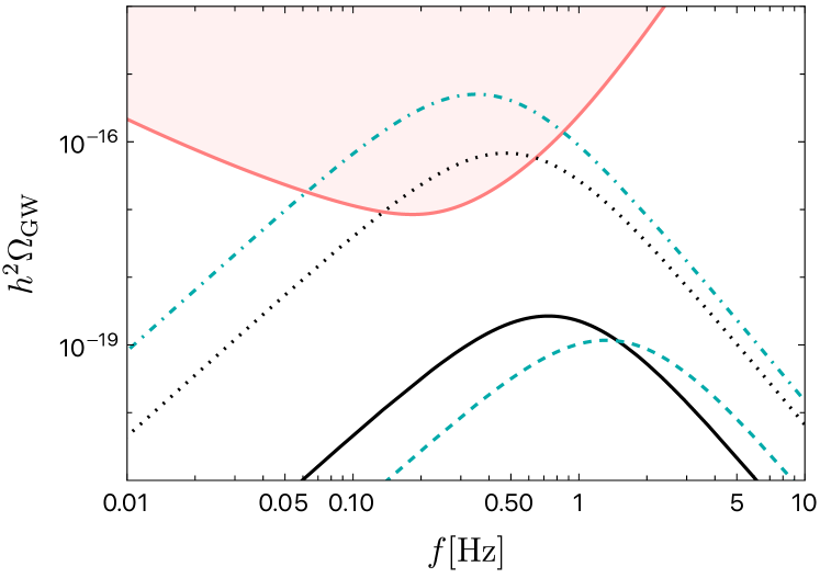
For comparison, we also consider a model with a large enthalpy jump, but no minimum temperature, and we choose $T_{n}/T_{c}=0.7$. Keeping $c_{s}^{2}=1/3$, we find $\xi_{w}=0.67$, and the GW spectrum is shown in black dotted. If we choose the same sound speed as in the dark SU(N) at $T_{n}$, $c_{s}^{2}=0.103$, we find that $\xi_{w}=0.90$, which enhances the GW spectrum by a factor $\sim 7$ and decreases the peak frequency by a factor 0.74 (cyan dot-dashed). For both graphs we used $\beta/H=6.8\times 10^{4}$ like in Morgante:2022zvc for large $\xi_{w}$.

V Conclusion

In this work we have explored the consequences of a large enthalpy jump, limited allowed temperature range and strong deviations from $c_{s}^{2}=1/3$ on the wall velocity and the predicted GW spectrum. Although these features arise naturally in holographic and strongly coupled theories, our results are also applicable to weakly coupled theories.

A large enthalpy-jump highly constrains the fluid flow, favoring deflagrations and hybrids over detonations, which cease to exist as the jump grows larger. It forces the fluid ahead of the wall to be at the critical temperature $T_{+}=T_{c}$ and to move at the same speed as the wall, $v_{+}=0$. By integrating the hydrodynamic equations (2) and solving matching conditions at the shock we showed that one can obtain a relation between the wall speed and the nucleation temperature depending solely on the EoS. Our estimate for the wall velocity becomes more accurate as the enthalpy jump increases in a given theory, as demonstrated in fig. 2. The method can be applied to bubbles in arbitrary dimensions. A formula to obtain $\xi_{w}$ was also proposed in Janik:2022wsx , but it has not yet been generalized beyond planar bubbles, and it only agrees with our result in the regime of small supercooling.

As discussed around eq. (13), the large $N$ limit also enforces local thermal equilibrium. This implies that as long as the enthalpy jump is large, the estimate of $\xi_{w}$ by the code snippet of Ai:2023see (developed for LTE) will be very similar to the one obtained with the method presented in this work.

We have pointed out that a limit on the amount of supercooling, rather than strong coupling, is the main limiting factor in obtaining fast walls. This clarifies the reason behind the low speeds measured in holographic simulations Bea:2021 ; Bea:2022 ; Janik:2022wsx . For illustration, we have computed the GW spectrum in the dark SU(N) model. We found that the limited temperature range indeed results in a small wall speed, which suppressed the GW spectrum compared to the case with a larger possibility for supercooling. We also demonstrated that non-conformal values of $c_{s}$, which naturally occur in holographic models, significantly affect the GW spectrum.

Our main conclusion is that care is needed when determining the wall speed in the computation of the GW spectrum. We have demonstrated a way of estimating the wall velocity in the case of a large enthalpy jump which can even be applied to strongly coupled theories and which should largely decrease the uncertainty in the GW prediction associated to $\xi_{w}$.

References

- (1) E. Witten, “Cosmic Separation of Phases,” Phys. Rev. D 30 (1984) 272–285.
- (2) A. Kosowsky, M. S. Turner, and R. Watkins, “Gravitational radiation from colliding vacuum bubbles,” Phys. Rev. D 45 (1992) 4514–4535.
- (3) A. Kosowsky, M. S. Turner, and R. Watkins, “Gravitational waves from first order cosmological phase transitions,” Phys. Rev. Lett. 69 (1992) 2026–2029.
- (4) M. Kamionkowski, A. Kosowsky, and M. S. Turner, “Gravitational radiation from first order phase transitions,” Phys. Rev. D 49 (1994) 2837–2851, arXiv:astro-ph/9310044.
- (5) C. Grojean and G. Servant, “Gravitational Waves from Phase Transitions at the Electroweak Scale and Beyond,” Phys. Rev. D 75 (2007) 043507, arXiv:hep-ph/0607107.
- (6) C. Caprini and D. G. Figueroa, “Cosmological Backgrounds of Gravitational Waves,” Class. Quant. Grav. 35 no. 16, (2018) 163001, arXiv:1801.04268 [astro-ph.CO].
- (7) C. Caprini et al., “Detecting gravitational waves from cosmological phase transitions with LISA: an update,” JCAP 03 (2020) 024, arXiv:1910.13125 [astro-ph.CO].
- (8) M. Hindmarsh, S. J. Huber, K. Rummukainen, and D. J. Weir, “Numerical simulations of acoustically generated gravitational waves at a first order phase transition,” Phys. Rev. D 92 no. 12, (2015) 123009, arXiv:1504.03291 [astro-ph.CO].
- (9) M. Hindmarsh, S. J. Huber, K. Rummukainen, and D. J. Weir, “Shape of the acoustic gravitational wave power spectrum from a first order phase transition,” Phys. Rev. D 96 no. 10, (2017) 103520, arXiv:1704.05871 [astro-ph.CO]. [Erratum: Phys.Rev.D 101, 089902 (2020)].
- (10) M. Hindmarsh, “Sound shell model for acoustic gravitational wave production at a first-order phase transition in the early Universe,” Phys. Rev. Lett. 120 no. 7, (2018) 071301, arXiv:1608.04735 [astro-ph.CO].
- (11) M. Hindmarsh and M. Hijazi, “Gravitational waves from first order cosmological phase transitions in the Sound Shell Model,” JCAP 12 (2019) 062, arXiv:1909.10040 [astro-ph.CO].
- (12) R. Jinno, T. Konstandin, and H. Rubira, “A hybrid simulation of gravitational wave production in first-order phase transitions,” JCAP 04 (2021) 014, arXiv:2010.00971 [astro-ph.CO].
- (13) R. Jinno, T. Konstandin, H. Rubira, and I. Stomberg, “Higgsless simulations of cosmological phase transitions and gravitational waves,” JCAP 02 (2023) 011, arXiv:2209.04369 [astro-ph.CO].
- (14) A. Roper Pol, S. Procacci, and C. Caprini, “Characterization of the gravitational wave spectrum from sound waves within the sound shell model,” arXiv:2308.12943 [gr-qc].
- (15) J. R. Espinosa, T. Konstandin, J. M. No, and G. Servant, “Energy Budget of Cosmological First-order Phase Transitions,” JCAP 06 (2010) 028, arXiv:1004.4187 [hep-ph].
- (16) F. Giese, T. Konstandin, and J. van de Vis, “Model-independent energy budget of cosmological first-order phase transitions—A sound argument to go beyond the bag model,” JCAP 07 no. 07, (2020) 057, arXiv:2004.06995 [astro-ph.CO].
- (17) F. Giese, T. Konstandin, K. Schmitz, and J. van de Vis, “Model-independent energy budget for LISA,” JCAP 01 (2021) 072, arXiv:2010.09744 [astro-ph.CO].
- (18) G. D. Moore and T. Prokopec, “How fast can the wall move? A Study of the electroweak phase transition dynamics,” Phys. Rev. D 52 (1995) 7182–7204, arXiv:hep-ph/9506475.
- (19) G. C. Dorsch, S. J. Huber, and T. Konstandin, “Bubble wall velocities in the Standard Model and beyond,” JCAP 12 (2018) 034, arXiv:1809.04907 [hep-ph].
- (20) M. Lewicki, M. Merchand, and M. Zych, “Electroweak bubble wall expansion: gravitational waves and baryogenesis in Standard Model-like thermal plasma,” JHEP 02 (2022) 017, arXiv:2111.02393 [astro-ph.CO].
- (21) B. Laurent and J. M. Cline, “First principles determination of bubble wall velocity,” Phys. Rev. D 106 no. 2, (2022) 023501, arXiv:2204.13120 [hep-ph].
- (22) S. Jiang, F. P. Huang, and X. Wang, “Bubble wall velocity during electroweak phase transition in the inert doublet model,” Phys. Rev. D 107 no. 9, (2023) 095005, arXiv:2211.13142 [hep-ph].
- (23) P. Schwaller, “Gravitational Waves from a Dark Phase Transition,” Phys. Rev. Lett. 115 no. 18, (2015) 181101, arXiv:1504.07263 [hep-ph].
- (24) S. Bruggisser, B. Von Harling, O. Matsedonskyi, and G. Servant, “Electroweak Phase Transition and Baryogenesis in Composite Higgs Models,” JHEP 12 (2018) 099, arXiv:1804.07314 [hep-ph].
- (25) W.-C. Huang, M. Reichert, F. Sannino, and Z.-W. Wang, “Testing the dark SU(N) Yang-Mills theory confined landscape: From the lattice to gravitational waves,” Phys. Rev. D 104 no. 3, (2021) 035005, arXiv:2012.11614 [hep-ph].
- (26) J. Halverson, C. Long, A. Maiti, B. Nelson, and G. Salinas, “Gravitational waves from dark Yang-Mills sectors,” JHEP 05 (2021) 154, arXiv:2012.04071 [hep-ph].
- (27) H. Yang, F. F. Freitas, A. Marciano, A. P. Morais, R. Pasechnik, and J. a. Viana, “Gravitational-wave signatures of chiral-symmetric technicolor,” Phys. Lett. B 830 (2022) 137162, arXiv:2204.00799 [hep-ph].
- (28) U. Gursoy, E. Kiritsis, L. Mazzanti, and F. Nitti, “Holography and Thermodynamics of 5D Dilaton-gravity,” JHEP 05 (2009) 033, arXiv:0812.0792 [hep-th].
- (29) U. Gursoy, E. Kiritsis, L. Mazzanti, and F. Nitti, “Improved Holographic Yang-Mills at Finite Temperature: Comparison with Data,” Nucl. Phys. B 820 (2009) 148–177, arXiv:0903.2859 [hep-th].
- (30) F. Bigazzi, A. Caddeo, A. L. Cotrone, and A. Paredes, “Fate of false vacua in holographic first-order phase transitions,” JHEP 12 (2020) 200, arXiv:2008.02579 [hep-th].
- (31) F. R. Ares, M. Hindmarsh, C. Hoyos, and N. Jokela, “Gravitational waves from a holographic phase transition,” JHEP 21 (2020) 100, arXiv:2011.12878 [hep-th].
- (32) F. Bigazzi, A. Caddeo, A. L. Cotrone, and A. Paredes, “Dark Holograms and Gravitational Waves,” JHEP 04 (2021) 094, arXiv:2011.08757 [hep-ph].
- (33) F. R. Ares, O. Henriksson, M. Hindmarsh, C. Hoyos, and N. Jokela, “Effective actions and bubble nucleation from holography,” Phys. Rev. D 105 no. 6, (2022) 066020, arXiv:2109.13784 [hep-th].
- (34) Z.-R. Zhu, J. Chen, and D. Hou, “Gravitational waves from holographic QCD phase transition with gluon condensate,” Eur. Phys. J. A 58 no. 6, (2022) 104, arXiv:2109.09933 [hep-ph].
- (35) E. Morgante, N. Ramberg, and P. Schwaller, “Gravitational waves from dark SU(3) Yang-Mills theory,” Phys. Rev. D 107 no. 3, (2023) 036010, arXiv:2210.11821 [hep-ph].
- (36) Y. Chen, D. Li, and M. Huang, “Bubble nucleation and gravitational waves from holography in the probe approximation,” JHEP 07 (2023) 225, arXiv:2212.06591 [hep-ph].
- (37) J. Casalderrey-Solana, D. Mateos, and M. Sanchez-Garitaonandia, “Mega-Hertz Gravitational Waves from Neutron Star Mergers,” arXiv:2210.03171 [hep-th].
- (38) Y. Bea, J. Casalderrey-Solana, T. Giannakopoulos, D. Mateos, M. Sanchez-Garitaonandia, and M. Zilhão, “Bubble wall velocity from holography,” Phys. Rev. D 104 (Dec, 2021) L121903. https://link.aps.org/doi/10.1103/PhysRevD.104.L121903.
- (39) Y. Bea, J. Casalderrey-Solana, T. Giannakopoulos, A. Jansen, D. Mateos, M. Sanchez-Garitaonandia, and M. Zilhão, “Holographic bubbles with Jecco: expanding, collapsing and critical,” JHEP 09 (2022) 008, arXiv:2202.10503 [hep-th]. [Erratum: JHEP 03, 225 (2023)].
- (40) F. Bigazzi, A. Caddeo, T. Canneti, and A. L. Cotrone, “Bubble wall velocity at strong coupling,” JHEP 08 (2021) 090, arXiv:2104.12817 [hep-ph].
- (41) R. A. Janik, M. Jarvinen, H. Soltanpanahi, and J. Sonnenschein, “Perfect Fluid Hydrodynamic Picture of Domain Wall Velocities at Strong Coupling,” Phys. Rev. Lett. 129 no. 8, (2022) 081601, arXiv:2205.06274 [hep-th].
- (42) Y. Bea and D. Mateos, “Heating up Exotic RG Flows with Holography,” JHEP 08 (2018) 034, arXiv:1805.01806 [hep-th].
- (43) D. Elander, A. F. Faedo, D. Mateos, and J. G. Subils, “Phase transitions in a three-dimensional analogue of Klebanov-Strassler,” JHEP 06 (2020) 131, arXiv:2002.08279 [hep-th].
- (44) L. D. Landau and E. M. Lifshitz, Fluid Mechanics. Pergamon Press, New York, 1989.
- (45) H. Kurki-Suonio and M. Laine, “Supersonic deflagrations in cosmological phase transitions,” Phys. Rev. D 51 (1995) 5431–5437, arXiv:hep-ph/9501216.
- (46) W.-Y. Ai, B. Laurent, and J. van de Vis, “Model-independent bubble wall velocities in local thermal equilibrium,” JCAP 07 (2023) 002, arXiv:2303.10171 [astro-ph.CO].
- (47) L. Leitao and A. Megevand, “Hydrodynamics of phase transition fronts and the speed of sound in the plasma,” Nucl. Phys. B 891 (2015) 159–199, arXiv:1410.3875 [hep-ph].
- (48) M. Barroso Mancha, T. Prokopec, and B. Swiezewska, “Field-theoretic derivation of bubble-wall force,” JHEP 01 (2021) 070, arXiv:2005.10875 [hep-th].
- (49) W.-Y. Ai, B. Garbrecht, and C. Tamarit, “Bubble wall velocities in local equilibrium,” JCAP 03 no. 03, (2022) 015, arXiv:2109.13710 [hep-ph].
- (50) J. Crowder and N. J. Cornish, “Beyond LISA: Exploring future gravitational wave missions,” Phys. Rev. D 72 (2005) 083005, arXiv:gr-qc/0506015.
- (51) V. Corbin and N. J. Cornish, “Detecting the cosmic gravitational wave background with the big bang observer,” Class. Quant. Grav. 23 (2006) 2435–2446, arXiv:gr-qc/0512039.
- (52) G. M. Harry, P. Fritschel, D. A. Shaddock, W. Folkner, and E. S. Phinney, “Laser interferometry for the big bang observer,” Class. Quant. Grav. 23 (2006) 4887–4894. [Erratum: Class.Quant.Grav. 23, 7361 (2006)].
- (53) K. Schmitz, “New Sensitivity Curves for Gravitational-Wave Signals from Cosmological Phase Transitions,” JHEP 01 (2021) 097, arXiv:2002.04615 [hep-ph].