Symbolic Numeric Planning with Patterns

Abstract

In this paper, we propose a novel approach for solving linear numeric planning problems, called Symbolic Pattern Planning. Given a planning problem $\Pi$, a bound $n$ and a pattern –defined as an arbitrary sequence of actions– we encode the problem of finding a plan for $\Pi$ with bound $n$ as a formula with fewer variables and/or clauses than the state-of-the-art rolled-up and relaxed-relaxed-$\exists$ encodings. More importantly, we prove that for any given bound, it is never the case that the latter two encodings allow finding a valid plan while ours does not. On the experimental side, we consider 6 other planning systems –including the ones which participated in this year’s International Planning Competition (IPC)– and we show that our planner Patty has remarkably good comparative performances on this year’s IPC problems.

Introduction

Planning is one of the oldest problems in Artificial Intelligence, see, e.g., (McCarthy and Hayes 1969). Starting from the classical setting in which all the variables are Boolean, in simple numeric planning problems variables can also range over the rationals and actions can increment or decrement their values by a fixed constant, while in linear numeric planning problems actions can also update variables to a new value which is a linear combination of the values of the variables in the state in which actions are executed, see, e.g., (Arxer and Scala 2023). Current approaches for solving a numeric planning problem $\Pi$ are either search-based (in which the state space is explored using techniques based on heuristic search, see, e.g., (Bonet and Geffner 2001)) or symbolic-based (in which a bound $n$ on the number of steps is a priori fixed and the problem of finding a plan with bound $n$ is encoded into a formula for which a decision procedure is available, see, e.g., (Kautz and Selman 1992)).

In this paper, we propose a novel symbolic approach for solving numeric planning problems, called symbolic pattern planning. Given a problem $\Pi$ and a pattern ${\prec}$ – defined as a sequence of actions – we show how it is possible to generalize the state-of-the-art rolled-up encoding $\Pi^{R}$ proposed in (Scala et al. 2016b) and the relaxed-relaxed-$\exists$ (${R^{2}\exists}{}$) encoding $\Pi^{R^{2}\exists}{}$ proposed in (Bofill, Espasa, and Villaret 2017), and define a new encoding $\Pi^{\prec}$ which provably dominates both $\Pi^{R}$ and $\Pi^{R^{2}\exists}{}$: for any bound $n$, it is never the case that the latter two allow to find a valid plan for $\Pi$ while ours does not. Further, our encoding produces formulas with fewer clauses than the rolled-up encoding and also with far fewer variables than the $R^{2}\exists$ encoding, even when considering a fixed bound. Most importantly, we believe that our proposal provides a new starting point for symbolic approaches: a pattern ${\prec}$ can be any sequence of actions (even with repetitions) and, assuming $n=1$, the formula produced by $\Pi^{\prec}$ encodes all the sequences of actions in which each action in ${\prec}$ is sequentially executed zero, one or possibly even more than one time. Thus, any planning problem can be solved with bound $n=1$ when considering a suitable pattern, and such pattern can be symbolically searched and incrementally defined also while increasing the bound, bridging the gap between symbolic and search-based planning.

To show the effectiveness of our proposal, we $(i)$ considered the 2 planners, benchmarks, and settings of the just concluded IPC, Agile track (Arxer and Scala 2023); and $(ii)$ added 4 other planning systems for both simple and linear numeric problems. Overall, our comparative analysis included 6 other planners, 3 of which symbolic and 3 search-based. The results show that, compared to the other symbolic planners, our planner Patty has always better performance on every domain, while compared to all the other planners, Patty has overall remarkably good performances, being the fastest system able to solve most problems on the largest number of domains.

The paper is structured as follows. After the preliminaries, we present the rolled-up, $R^{2}\exists$ and our pattern encodings, and prove that the latter dominates the previous two. Then, the experimental analysis and the conclusion follow. One running example is used throughout the paper to illustrate the formal definitions and the theoretical results.

Preliminaries

We consider a fragment of numeric planning expressible with PDDL2.1, level 2 (Fox and Long 2003). A numeric planning problem is a tuple $\Pi=\langle V_{B},V_{N},A,I,G\rangle$, where $V_{B}$ and $V_{N}$ are finite sets of Boolean and numeric variables with domains $\{\top,\bot\}$ and $\mathbb{Q}$, respectively ($\top$ and $\bot$ are the symbols we use for truth and falsity). $I$ is the initial state mapping each variable to an element in its domain. A propositional condition for a variable $v\in V_{B}$ is either $v=\top$ or $v=\bot$, while a numeric condition has the form $\psi\unrhd 0$, where $\unrhd\in\{\geq,>,=\}$ and $\psi$ is a linear expression over $V_{N}$, i.e., is equal to $\sum_{w\in V_{N}}k_{w}w+k$, for some $k_{w},k\in\mathbb{Q}$. $G$ is a finite set of goal formulas, each one being a propositional combination of propositional and numeric conditions. Finally, $A$ is a finite set of actions. An action $a$ is a pair $\langle\mathrm{pre}(a),\mathrm{eff}(a)\rangle$ in which $(i)$ $\mathrm{pre}(a)$ is the union of the sets of propositional and numeric preconditions of $a$, represented as propositional and numeric conditions, respectively; and $(ii)$ $\mathrm{eff}(a)$ is the union of the sets of propositional and numeric effects, the former of the form $v:=\top$ or $v:=\bot$, the latter of the form $w:=\psi$, with $v\in V_{B}$, $w\in V_{N}$ and $\psi$ a linear expression. We assume that for each action $a$ and variable $v\in V_{B}\cup V_{N}$, $v$ occurs in $\mathrm{eff}(a)$ at most once to the left of the operator “$:=$”, and when this happens we say that $v$ is assigned by $a$. In the rest of the paper, $v,w,x,y$ denote variables, $a,b$ denote actions and $\psi$ denotes a linear expression, each symbol possibly decorated with subscripts.

Example.

There are two robots $l$ and $r$ for left and right, respectively, whose position $x_{l}$ and $x_{r}$ on an axis correspond to the integers $\leq 0$ and $\geq 0$, respectively. The two robots can move to the left or to the right, decreasing or increasing their position by 1. The two robots carry $q_{l}$ and $q_{r}$ objects, which they can exchange. However, before exchanging objects at rate $q$, the two robots must connect setting a Boolean variable $p$ to $\top$, and this is possible only if they have the same position. Once connected, they must disconnect before moving again. The quantity $q$ can be positive or negative, corresponding to $l$ giving objects to $r$ or vice versa. This scenario can be modelled in PDDL with $V_{B}=\{p\}$, $V_{N}=\{x_{l},x_{r},q_{l},q_{r},q\}$ and the following set of actions:

$$\begin{array}[]{c}\texttt{lft}_{r}:\langle\{x_{r}>0\},\{x_{r}\mathrel{-}=1\}\rangle,\ \texttt{rgt}_{r}:\langle\{p=\bot\},\{x_{r}\mathrel{+}=1\}\rangle,\\ \texttt{lft}_{l}:\langle\{p=\bot\},\{x_{l}\mathrel{-}=1\}\rangle,\ \texttt{rgt}_{l}:\langle\{x_{l}<0\},\{x_{l}\mathrel{+}=1\}\rangle,\\ \texttt{conn}:\langle\{x_{l}=x_{r}\},\{p:=\top\}\rangle,\ \texttt{disc}:\langle\{p=\top\},\{p:=\bot\}\rangle,\\ \texttt{exch}:\langle\{p=\top,q_{l}\geq q,q_{r}\geq-q\},\{q_{l}\mathrel{-}=q,q_{r}\mathrel{+}=q\}\rangle,\\ \texttt{lre}:\langle\{\},\{q:=1\}\rangle,\texttt{rle}:\langle\{\},\{q:=-1\}\rangle.\end{array}$$ (1)

As customary, $v\mathrel{+}=\psi$ is an abbreviation for $v:=v+\psi$ and similarly for $v\mathrel{-}=\psi$ and we abbreviate $-\psi>0$ with the equivalent $\psi<0$.

Let $\Pi=\langle V_{B},V_{N},A,I,G\rangle$ be a numeric planning problem. A state $s$ maps each variable $v\in V_{B}\cup V_{N}$ to a value $s(v)$ in its domain, and is extended to linear expressions, Boolean and numeric conditions and their propositional combinations. An action $a\in A$ is executable in a state $s$ if $s$ satisfies all the preconditions of $a$. Given a state $s$ and an executable action $a$, the result of executing $a$ in $s$ is the state $s^{\prime}$ such that for each variable $v\in V_{B}\cup V_{N}$,

1. $s^{\prime}(v)=\top$ if $v:=\top\in\mathrm{eff}(a)$, $s^{\prime}(v)=\bot$ if $v:=\bot\in\mathrm{eff}(a)$, $s^{\prime}(v)=s(\psi)$ if $(v:=\psi)\in\mathrm{eff}(a)$, and

2. $s^{\prime}(v)=s(v)$ otherwise.

Given a finite sequence $\alpha$ of actions $a_{0};\ldots;a_{n-1}$ of length $n\geq 0$, the state sequence $s_{0};\ldots;s_{n}$ induced by $\alpha$ in $s_{0}$ is such that for $i\in[0,n)$, $s_{i+1}$ $(i)$ is undefined if either $a_{i}$ is not executable in $s_{i}$ or $s_{i}$ is undefined, and $(ii)$ is the result of executing $a_{i}$ in $s_{i}$ otherwise.

Consider a finite sequence of actions $\alpha$. We say that $\alpha$ is executable in a state $s_{0}$ if each state in the sequence induced by $\alpha$ in $s_{0}$ is defined. If $\alpha$ is executable in the initial state $I$ and the last state induced by $\alpha$ in $I$ satisfies the goal formulas in $G$, we say that $\alpha$ is a (valid) plan. In the following, we will use $\alpha$ and $\pi$ to, respectively, denote a generic sequence of actions and a plan, possibly decorated with subscripts. For an action $a$ and $k\in\mathbb{N}$, $a^{k}$ denotes the sequence consisting of the action $a$ repeated $k$ times.

Example (cont’d).

Assume the initial state is $I=\{p=\bot,x_{l}=-X_{I},x_{r}=X_{I},q_{l}=Q,q_{r}=0,q=1\}$, where $X_{I},Q$ are positive integers. Assuming $G=\{q_{l}=0,q_{r}=Q,x_{l}=-X_{I},x_{r}=X_{I}\}$, one of the shortest plans is

$$\!\!\texttt{rgt}_{l}^{X_{I}};\texttt{lft}_{r}^{X_{I}};\texttt{conn};\texttt{exch}^{Q};\texttt{disc};\texttt{lft}_{l}^{X_{I}};\texttt{rgt}_{r}^{X_{I}}\!$$ (2)

corresponding to the robots going to the origin, connect, exchange the $Q$ items, disconnect, and then go back to their initial positions.

Symbolic Planning With Patterns

Symbolic Planning

Let $\Pi=\langle V_{B},V_{N},A,I,G\rangle$ be a numeric planning problem.

An encoding $\Pi^{E}$ of $\Pi$ is a 5-tuple $\Pi^{E}=\langle\mathcal{X},\mathcal{A},\mathcal{I}(\mathcal{X}),\mathcal{T}(\mathcal{X},\mathcal{A},\mathcal{X}^{\prime}),\mathcal{G}(\mathcal{X})\rangle$ where

1. $\mathcal{X}$ is a finite set of state variables, each one equipped with a domain representing the values it can take. We assume $V_{B}\cup V_{N}\subseteq\mathcal{X}$.

2. $\mathcal{A}$ is a finite set of action variables, each one equipped with a domain representing the values it can take.

3. $\mathcal{I}(\mathcal{X})$ is the initial state formula, a formula in the set $\mathcal{X}$ of variables defined as

   $$\bigwedge_{v:I(v)=\bot}\neg v\wedge\bigwedge_{w:I(w)=\top}w\wedge\bigwedge_{x,k:I(x)=k}x=k.$$

4. $\mathcal{T}(\mathcal{X},\mathcal{A},\mathcal{X}^{\prime})$ is the symbolic transition relation, a formula in the variables $\mathcal{X}\cup\mathcal{A}\cup\mathcal{X}^{\prime}$, where $\mathcal{X}^{\prime}$ is a copy of $\mathcal{X}$. Together with $\mathcal{T}(\mathcal{X},\mathcal{A},\mathcal{X}^{\prime})$, a decoding function has to be defined enabling to associate to each model of $\mathcal{T}(\mathcal{X},\mathcal{A},\mathcal{X}^{\prime})$ at least one sequence of actions in $A$. Standard requirements for $\mathcal{T}(\mathcal{X},\mathcal{A},\mathcal{X}^{\prime})$ are:

   1. correctness: for each sequence of actions $\alpha$ corresponding to a model $\mu$ of $\mathcal{T}(\mathcal{X},\mathcal{A},\mathcal{X}^{\prime})$, $(i)$ $\alpha$ is executable in the state $s$ in which, for each variable $v\in V_{B}\cup V_{N}$, $s(v)=\mu(v)$; and $(ii)$ the last state induced by $\alpha$ executed in $s$ is the state $s^{\prime}$ such that, for each variable $v\in V_{B}\cup V_{N}$, $s^{\prime}(v)=\mu(v^{\prime})$;

   2. completeness: for each state $s$ and action $a\in A$ executable in $s$ with resulting state $s^{\prime}$, there must be a model $\mu$ of $\mathcal{T}(\mathcal{X},\mathcal{A},\mathcal{X}^{\prime})$ such that, for each state variable $v\in V_{B}\cup V_{N}$, $\mu(v)=s(v)$, $\mu(v^{\prime})=s^{\prime}(v)$ and the sequence of actions containing only $a$ corresponds to $\mu$.

5. $\mathcal{G}(\mathcal{X})$ is the goal formula, obtained by making the conjunction of the formulas in $G$, once $v=\top$ and $v=\bot$ are substituted with $v$ and $\neg v$, respectively.

Example (cont’d).

The initial state and goal formulas are $(\neg p\wedge x_{l}=-X_{I}\wedge x_{r}=X_{I}\wedge q_{l}=Q\wedge q_{r}=0\wedge q=1)$ and $(q_{l}=0\wedge q_{r}=Q\wedge x_{l}=-X_{I}\wedge x_{r}=X_{I})$, respectively.

Let $\Pi^{E}=\langle\mathcal{X},\mathcal{A},\mathcal{I}(\mathcal{X}),\mathcal{T}(\mathcal{X},\mathcal{A},\mathcal{X}^{\prime}),\mathcal{G}(\mathcal{X})\rangle$ be an encoding of $\Pi$. As in the planning as satisfiability approach (Kautz and Selman 1992), we fix an integer $n\geq 0$ called bound or number of steps, we make $n+1$ disjoint copies $\mathcal{X}_{0},\ldots,\mathcal{X}_{n}$ of the set $\mathcal{X}$ of state variables, and $n$ disjoint copies $\mathcal{A}_{0},\ldots,\mathcal{A}_{n-1}$ of the set $\mathcal{A}$ of action variables, and define

1. $\mathcal{I}(\mathcal{X}_{0})$ as the formula in the variables $\mathcal{X}_{0}$ obtained by substituting each variable $x\in\mathcal{X}$ with $x_{0}\in\mathcal{X}_{0}$ in $\mathcal{I}(\mathcal{X})$;

2. for each step $i=0,\ldots,n-1$, $\mathcal{T}(\mathcal{X}_{i},\mathcal{A}_{i},\mathcal{X}_{i+1})$ as the formula in the variables $\mathcal{X}_{i}\cup\mathcal{A}_{i}\cup\mathcal{X}_{i+1}$ obtained by substituting each variable $x\in\mathcal{X}$ (resp. $a\in\mathcal{A}$, $x^{\prime}\in\mathcal{X}^{\prime}$) with $x_{i}\in\mathcal{X}_{i}$ (resp. $a_{i}\in\mathcal{A}_{i}$, $x_{i+1}\in\mathcal{X}_{i+1}$) in $\mathcal{T}(\mathcal{X},\mathcal{A},\mathcal{X}^{\prime})$;

3. $\mathcal{G}(\mathcal{X}_{n})$ as the formula in the variables $\mathcal{X}_{n}$ obtained by substituting each variable $x\in\mathcal{X}$ with $x_{n}\in\mathcal{X}_{n}$ in $\mathcal{G}(\mathcal{X})$.

Then, the encoding $\Pi^{E}$ of $\Pi$ with bound $n$ is the formula

$$\Pi^{E}_{n}=\mathcal{I}(\mathcal{X}_{0})\wedge\bigwedge_{i=0}^{n-1}\mathcal{T}(\mathcal{X}_{i},\mathcal{A}_{i},\mathcal{X}_{i+1})\wedge\mathcal{G}(\mathcal{X}_{n}).$$ (3)

To each model $\mu$ of $\Pi^{E}_{n}$, we associate the set of sequences of actions $\alpha_{0};\ldots;\alpha_{n-1}$, where each $\alpha_{i}$ is a sequence of actions corresponding to the model of $\mathcal{T}(\mathcal{X}_{i},\mathcal{A}_{i},\mathcal{X}_{i+1})$ obtained by restricting $\mu$ to $\mathcal{X}_{i}\cup\mathcal{A}_{i}\cup\mathcal{X}_{i+1}$, $i\in[0,n)$. In the following, $(\Pi^{E}_{n})\raisebox{4.95134pt}{$\scriptscriptstyle-\!1$}$ is the set of sequences of actions in $A$ associated to a model of $\Pi^{E}_{n}$. The correctness of $\mathcal{T}(\mathcal{X},\mathcal{A},\mathcal{X}^{\prime})$ ensures the correctness of $\Pi^{E}$: for each bound $n$, each sequence in $(\Pi^{E}_{n})\raisebox{4.95134pt}{$\scriptscriptstyle-\!1$}$ is a plan. The completeness of $\mathcal{T}(\mathcal{X},\mathcal{A},\mathcal{X}^{\prime})$ ensures the completeness of $\Pi^{E}$: if it exists a plan for $\Pi$, it will be found by considering $\Pi^{E}_{0}$, $\Pi^{E}_{1}$, ….

It is clear that the number of variables and size of (3) increase with the bound $n$, explaining why much of the research has concentrated on how to produce encodings allowing to find plans with the lowest possible bound $n$.

Rolled-up, Standard and $R^{2}\exists$ Encodings

Let $\Pi=\langle V_{B},V_{N},A,I,G\rangle$ be a numeric planning problem. Many encodings have been proposed, each characterized by how the symbolic transition relation is computed. In most encodings (see, e.g., (Rintanen, Heljanko, and Niemelä 2006; Bofill, Espasa, and Villaret 2017; Leofante et al. 2020)), each action $a\in A$ is defined as a Boolean variable in $\mathcal{A}$ which will be true (resp. false) in a model $\mu$ of $\mathcal{T}(\mathcal{X},\mathcal{A},\mathcal{X}^{\prime})$ if action $a$ occurs once (resp. does not occur) in each sequence of actions corresponding to $\mu$. Here we start presenting the state-of-the-art rolled-up encoding $\Pi^{R}$ of $\Pi$ proposed by (Scala et al. 2016b). In $\Pi^{R}$, each action $a\in A$ is defined as an action variable which can get an arbitrary value $k\in\mathbb{N}$, and this corresponds to have $k$ (consecutive) occurrences of $a$ in the action sequences corresponding to the models of the symbolic transition relation of $\Pi^{R}$. However, in $\Pi^{R}$ it is not the case that each action $a$ can get a value $>1$, (e.g., because $a$ cannot be executed more than once, or it is not useful to execute $a$ more than once), and the definition of when it is possible to set $a>1$ depends on the form of the effects of $a$. For this reason, each effect $v:=e$ of an action $a$ is categorized as

1. a Boolean assignment, if $v\in V_{B}$ and $e\in\{\top,\bot\}$, as for the effects of the actions conn and disc in (1), or as

2. a linear increment, if $e=v+\psi$ with $\psi$ a linear expression not containing any of the variables assigned by $a$, as for the effects of the action exch and $\texttt{lft}_{r}$ in (1), or as

3. a general assignment, if it does not fall in the above two categories. General assignments are further divided into

   1. simple assignments, when $e$ does not contain any of the variables assigned by $a$, as in the effects of the actions lre and rle in (1), and

   2. self-interfering assignments, otherwise.

Then, an action $a$ is eligible for rolling if

1. $v=\bot\in\mathrm{pre}(a)$ (resp. $v=\top\in\mathrm{pre}(a)$) implies $v:=\top\not\in\mathrm{eff}(a)$ (resp. $v:=\bot\not\in\mathrm{eff}(a)$), and

2. $a$ does not contain a self-interfering assignment, and

3. $a$ contains a linear increment.

The result of rolling action $a$ for $k\geq 1$ times is such that

1. if $v\mathrel{+}=\psi\in\texttt{eff}(a)$ is a linear increment, then the value of $v$ is incremented by $k\times\psi$, while

2. if $v:=e\in\texttt{eff}(a)$ is a Boolean or simple assignment, then the value of $v$ becomes $e$, equal to the value obtained after a single execution of $a$.

On the other hand, if an action $a$ is not eligible for rolling, $a>1$ is not allowed, and this can be enforced through at-most-once (“amo”) axioms.

In $\Pi^{R}$, the symbolic transition relation $\mathcal{T}^{R}(\mathcal{X},\mathcal{A},\mathcal{X}^{\prime})$ is the conjunction of the formulas in the following sets:

1. $\mathrm{pre}^{R}(A)$, consisting of, for each $a\in A$, $v=\bot$ and $w=\top$ in $\mathrm{pre}(a)$,

   $$a>0\rightarrow(\neg v\wedge w),$$

   and, for each $a\in A$ and $\psi\unrhd 0$ in $\mathrm{pre}(a)$,

   $$a>0\rightarrow\psi\unrhd 0,\qquad a>1\rightarrow\psi[a]\unrhd 0,$$

   where $\psi[a]$ is the linear expression obtained from $\psi$ by substituting each variable $x$ with

   1. $x+(a-1)\times\psi_{1}$, whenever $x\mathrel{+}=\psi_{1}\in\texttt{eff}(a)$ is a linear increment,

   2. $\psi_{1}$, if $x:=\psi_{1}\in\mathrm{eff}(a)$ is a simple assignment.

   The last two formulas ensure that $\psi\unrhd 0$ holds in the states in which the first and the last execution of $a$ happens (see (Scala et al. 2016b)).

2. $\mathrm{eff}^{R}(A)$, consisting of, for each $a\in A$, $v:=\bot$, $w:=\top$, linear increment $x\mathrel{+}=\psi$ and general assignment $y:=\psi_{1}$ in $\mathrm{eff}(a)$,

   $$a>0\rightarrow(\neg v^{\prime}\wedge w^{\prime}\wedge x^{\prime}=x+a\times\psi\wedge y^{\prime}=\psi_{1}).$$

3. $\mathrm{frame}^{R}(V_{B}\cup V_{N})$, consisting of, for each variable $v\in V_{B}$ and $w\in V_{N}$,

   $$\begin{array}[]{c}\!\!\!(\bigwedge_{a:v:=\top\in\mathrm{eff}(a)}a=0\wedge\bigwedge_{a:v:=\bot\in\mathrm{eff}(a)}a=0)\rightarrow v^{\prime}\equiv v,\\ \bigwedge_{a:w:=\psi\in\mathrm{eff}(a)}a=0\rightarrow w^{\prime}=w.\end{array}$$

4. $\mathrm{mutex}^{R}(A)$ consisting of $(a_{1}=0\vee a_{2}=0),$ for each pair of distinct actions $a_{1}$ and $a_{2}$ such that there exists a variable $v$ with

   1. $v\in V_{B}$, $v=\bot$ (resp. $v=\top$) in $\mathrm{pre}(a_{1})$ and $v:=\top$ (resp. $v:=\bot$) in $\mathrm{eff}(a_{2})$, or

   2. $v\in V_{N}$, $v:=\psi\in\texttt{eff}(a_{1})$ and $v$ occurring either in $\texttt{eff}(a_{2})$ or in $\texttt{pre}(a_{2})$.

5. $\mathrm{amo}^{R}(A)$ consisting of, for each action $a$ not eligible for rolling,

   $$(a=0\vee a=1).$$

Notice that if for action $a$ the formula $(a=0\vee a=1)$ belongs to $\mathcal{T}^{R}(\mathcal{X},\mathcal{A},\mathcal{X}^{\prime})$, we can equivalently $(i)$ define $a$ to be a Boolean variable, and then $(ii)$ replace $a=0$, $a>0$, $a=1$ and $a>1$ with $\neg a$, $a$, $a$ and $\bot$, respectively, in $\mathcal{T}^{R}(\mathcal{X},\mathcal{A},\mathcal{X}^{\prime})$. It is clear that if $\mathcal{T}^{R}(\mathcal{X},\mathcal{A},\mathcal{X}^{\prime})$ contains $(a=0\vee a=1)$ for any action $a$, then the rolled-up encoding $\Pi^{R}$ reduces to the standard encoding as defined, e.g., in (Leofante et al. 2020). Equivalently, in the standard encoding $\Pi^{S}$ of $\Pi$, the symbolic transition relation $\mathcal{T}^{S}(\mathcal{X},\mathcal{A},\mathcal{X}^{\prime})$ is obtained by adding, for each action $a$, $(a=0\vee a=1)$ to $\mathcal{T}^{R}(\mathcal{X},\mathcal{A},\mathcal{X}^{\prime})$. The decoding function of the rolled-up (resp. standard) encoding associates to each model $\mu$ of $\mathcal{T}^{R}(\mathcal{X},\mathcal{A},\mathcal{X}^{\prime})$ (resp. $\mathcal{T}^{S}(\mathcal{X},\mathcal{A},\mathcal{X}^{\prime})$) the sequences of actions in which each action $a$ occurs $\mu(a)$ times.

The biggest problem with the rolled-up and standard encodings is the presence of the axioms in $\mathrm{mutex}(A)$, which $(i)$ cause the size of $\mathcal{T}^{R}(\mathcal{X},\mathcal{A},\mathcal{X}^{\prime})$ to be possibly quadratic in the size of $\Pi$; and $(ii)$ forces some actions to be set to $0$ even when it is not necessary to maintain the correctness and completeness of $\mathcal{T}^{R}(\mathcal{X},\mathcal{A},\mathcal{X}^{\prime})$, see, e.g., (Rintanen, Heljanko, and Niemelä 2006). Indeed, allowing to set more actions to a value $>0$ while maintaining correctness and completeness, allows finding solutions to (3) with a lower value for the bound. Several proposals along these lines have been made. Here we present the $R^{2}\exists$ encoding presented in (Bofill, Espasa, and Villaret 2017) which is arguably the state-of-the-art encoding in which actions are encoded as Boolean variables (though there exist cases in which the $\exists$-encoding presented in (Rintanen, Heljanko, and Niemelä 2006) allows to solve (3) with a value for the bound lower than the one needed by the $R^{2}\exists$ encoding).

In the $R^{2}\exists$ encoding, action variables are Boolean and assumed to be ordered according to a given total order $\mathrel{<}$. In general, different orderings lead to different $R^{2}\exists$ encodings. In the following, we represent and reason about $\mathrel{<}$ considering the corresponding sequence of actions (which indeed contains each action in $A$ exactly once) and define $\Pi^{<}$ to be the $R^{2}\exists$ $<$-encoding of $\Pi$. In $\Pi^{<}$, for each action $a$ and variable $v$ assigned by $a$, a newly introduced variable $v^{a}$ with the same domain of $v$ is added to the set $\mathcal{X}$ of state variables. Intuitively, each new variable $v^{a}$ represents the value of $v$ after the sequential execution of some actions in the initial sequence of $<$ ending with $a$. The symbolic transition relation $\mathcal{T}^{<}(\mathcal{X},\mathcal{A},\mathcal{X}^{\prime})$ of $\Pi^{<}$ is the conjunction of the formulas in the following sets:

1. $\mathrm{pre}^{<}(A)$, consisting of, for each $a\in A$, $v=\bot$, $w=\top$ and $\psi\unrhd 0$ in $\mathrm{pre}(a)$,

   $$a\rightarrow(\neg v^{\ll,a}\wedge w^{\ll,a}\wedge\psi^{\ll,a}\unrhd 0),$$

   where, for each variable $x\in V_{B}\cup V_{N}$, $x^{\ll,a}$ stands for the variable $(i)$ $x$, if there is no action preceding $a$ in $<$ assigning $x$; and $(ii)$ $x^{b}$, if $b$ is the last action assigning $x$ preceding $a$ in $<$. Analogously, $\psi^{\ll,a}$ is the linear expression obtained from $\psi$ by substituting each variable $x\in V_{N}$ with $x^{\ll,a}$.

2. $\mathrm{eff}^{<}(A)$, consisting of, for each $a\in A$, $v:=\bot$, $w:=\top$ and general assignment $x:=\psi$ in $\mathrm{eff}(a)$,

   $$\begin{array}[]{cc}a\rightarrow(\neg v^{a}\wedge w^{a}\wedge x^{a}=\psi^{\ll,a}),\\ \neg a\rightarrow(v^{a}\leftrightarrow v^{\ll,a}\wedge w^{a}\leftrightarrow w^{\ll,a}\wedge x^{a}=x^{\ll,a}).\end{array}$$

3. $\mathrm{frame}^{<}(V_{B}\cup V_{N})$, consisting of, for each variable $v\in V_{B}$ and $w\in V_{N}$,

   $$v^{\prime}\leftrightarrow v^{\ll,g},\qquad w^{\prime}=w^{\ll,g},$$

   where $g$ is a dummy action assumed to follow all the other actions in $<$.

The decoding function of the $R^{2}\exists$ $<$-encoding associates to each model $\mu$ of $\mathcal{T}^{<}(\mathcal{X},\mathcal{A},\mathcal{X}^{\prime})$ the sequence of actions obtained from $<$ by deleting the actions $a$ with $\mu(a)=\bot$. In the $R^{2}\exists$ $<$-encoding, there are no mutex axioms and the size of $\mathcal{T}^{<}(\mathcal{X},\mathcal{A},\mathcal{X}^{\prime})$ is linear in the size of $\Pi$. However, as we mentioned previously, it introduces many new state variables (in the worst case, $|V_{B}\cup V_{N}|\times|A|$).

The main advantage of $\Pi^{R}$ and $\Pi^{<}$ over $\Pi^{S}$ is that the first two allow to find plans with lower values for the bound.

Example (cont’d).

The rolled-up (resp. standard) encoding of the two robots problem admits a model with bound $n=5$ (resp. $n=2X_{I}+Q+2$, and thus $n=5$ when $X_{I}=Q=1$). The $R^{2}\exists$ $<$-encoding admits a model with bound $n=2(X_{I}-1)+Q$ if actions in $<$ are ordered as in the plan (2), and thus $n=1$ when $X_{I}=Q=1$. In the worst case, the $R^{2}\exists$ $<$-encoding admits a solution with a bound equal to the one needed by the standard encoding, and this happens when actions in $<$ are in reverse order wrt the plan (2).

As the example shows, $\Pi^{R}$ and $\Pi^{<}$ dominate $\Pi^{S}$, while $\Pi^{R}$ and $\Pi^{<}$ do not dominate each other. Given two correct encodings $\Pi^{E_{1}}$ and $\Pi^{E_{2}}$ of $\Pi$, $\Pi^{E_{1}}$ dominates $\Pi^{E_{2}}$ if for any bound $n$, $\Pi^{E_{2}}_{n}$ satisfiability implies $\Pi^{E_{1}}_{n}$ satisfiability.

Theorem 1.

Let $\Pi$ be a numeric planning problem. Let $<$ be a total order of actions. The rolled-up encoding $\Pi^{R}$, the $R^{2}\exists$ $<$-encoding $\Pi^{<}$ and the standard encoding $\Pi^{S}$ of $\Pi$ are correct and complete. $\Pi^{R}$ and $\Pi^{<}$ dominate $\Pi^{S}$.

Proof.

(Sketch) For the correctness of $\Pi^{R}$ (and thus of $\Pi^{S}$) and $\Pi^{<}$ see Prop. 3 and Theorem 1 in the respective original papers. The completeness of $\Pi^{S}$ is taken for granted. A model of $\Pi_{n}^{S}$ with a corresponding plan $\pi$ is also a model of $\Pi_{n}^{R}$, and can be easily used to define a model of $\Pi_{n}^{<}$ with the same corresponding plan $\pi$. This implies the completeness of $\Pi^{R}$ and $\Pi^{<}$ and the fact that they dominate $\Pi^{S}$. ∎

Pattern Encoding

Let $\Pi=\langle V_{B},V_{N},A,I,G\rangle$ be a numeric planning problem. In the pattern encoding we combine and then generalize the strengths of the rolled-up and $R^{2}\exists$ encoding by $(i)$ allowing for the multiple executions of actions; $(ii)$ considering an ordering to avoid mutexes; and $(iii)$ allowing for arbitrary sequences of actions.

Consider a pattern ${\prec}$, defined as a possibly empty, finite sequence of actions. In the pattern ${\prec}$-encoding $\Pi^{\prec}$ of $\Pi$,

1. $\mathcal{X}=V_{B}\cup V_{N}\cup V$, where $V$ contains a newly introduced variable $v^{{\prec}_{1};a}$ with the same range of $v$, for each variable $v$ and initial pattern ${\prec}_{1};a$ of ${\prec}$ (i.e., ${\prec}$ starts with ${\prec}_{1};a$) in which $a$ contains a general assignment of $v$, and

2. $\mathcal{A}$ contains one action variable $a^{{\prec}_{1}}$ ranging over $\mathbb{N}$, for each initial pattern ${\prec}_{1};a$ of ${\prec}$.

Then, the value of a variable $v\in V_{B}\cup V_{N}$ after one or more of the actions in ${\prec}$ are executed (possibly consecutively multiple times) is given by $\sigma^{\prec}(v)$, where $\sigma^{\prec}(v)$ is inductively defined as $(i)$ $\sigma^{{\prec}}(v)=v$ if ${\prec}$ is the empty sequence; and $(ii)$ for a non-empty pattern ${\prec}={\prec}_{1};a$,

1. if $v$ is not assigned by $a$, $\sigma^{{\prec}}(v)=\sigma^{{\prec}_{1}}(v)$;

2. if $v:=\top\in\mathrm{eff}(a)$, $\sigma^{{\prec}}(v)=(\sigma^{{\prec}_{1}}(v)\vee a>0)$;

3. if $v:=\bot\in\mathrm{eff}(a)$, $\sigma^{{\prec}}(v)=(\sigma^{{\prec}_{1}}(v)\wedge a=0)$;

4. if $v\mathrel{+}=\psi\in\mathrm{eff}(a)$ is a linear increment, $\sigma^{{\prec}}(v)=\sigma^{{\prec}_{1}}(v)+a\times\sigma^{{\prec}_{1}}(\psi)$;

5. if $v:=\psi\in\mathrm{eff}(a)$ is a general assignment $\sigma^{{\prec}}(v)=v^{{\prec}}$.

Above and in the following, for any pattern ${\prec}_{1}$ and linear expression $\psi$, $\sigma^{{\prec}_{1}}(\psi)$ is the expression obtained by substituting each variable $v\in V_{N}$ in $\psi$ with $\sigma^{{\prec}_{1}}(v)$.

Example (cont’d).

Consider (1), and assume ${\prec}$ is

$$\texttt{lre};\texttt{rle};\texttt{lft}_{r};\texttt{rgt}_{l};\texttt{conn};\texttt{exch};\texttt{disc};\texttt{rgt}_{r};\texttt{lft}_{l}.$$

We have two newly introduced variables $q^{lre}$ and $q^{lre;rle}$, and for the Boolean variable $p$,

$$\sigma^{\prec}(p)=(p\vee\texttt{conn}>0)\wedge\texttt{disc}=0,$$

and, for the numeric variables in $V_{N}=\{x_{l},x_{r},q_{l},q_{r},q\}$,

$$\begin{array}[]{cc}\sigma^{\prec}(x_{l})=x_{l}+\texttt{rgt}_{l}-\texttt{lft}_{l},\\ \sigma^{\prec}(x_{r})=x_{r}-\texttt{lft}_{r}+\texttt{rgt}_{r},\\ \sigma^{\prec}(q_{l})=q_{l}-\texttt{exch}\times q^{lre;rle},\\ \sigma^{\prec}(q_{r})=q_{r}+\texttt{exch}\times q^{lre;rle},\\ \sigma^{\prec}(q)=q^{\texttt{lre;rle}}.\end{array}$$

The symbolic transition relation $\mathcal{T}^{\prec}(\mathcal{X},\mathcal{A},\mathcal{X}^{\prime})$ of $\Pi^{\prec}$ is the conjunction of the formulas in the following sets:

1. $\mathrm{pre}^{\prec}(A)$, which contains, for each initial pattern ${\prec}_{1};a$ of ${\prec}$, and for each $v=\bot$ and $w=\top$ in $\mathrm{pre}(a)$,

   $$\begin{array}[]{c}a^{{\prec}_{1}}>0\rightarrow(\neg\sigma^{{\prec}_{1}}(v)\wedge\sigma^{{\prec}_{1}}(w)),\end{array}$$

   and, for each numeric precondition $\psi\unrhd 0$ in $\mathrm{pre}(a)$,

   $$\begin{array}[]{c}a^{{\prec}_{1}}>0\rightarrow\sigma^{{\prec}_{1}}(\psi)\unrhd 0,\ \ a^{{\prec}_{1}}>1\rightarrow\sigma^{{\prec}_{1}}(\psi[a])\unrhd 0.\end{array}$$

2. $\mathrm{eff}^{\prec}(A)$, consisting of, for each initial pattern ${\prec}_{1};a$ of ${\prec}$ and variable $v$ such that $v:=\psi\in\mathrm{eff}(a)$ is a general assignment,

   $$\begin{array}[]{c}a^{{\prec}_{1}}=0\rightarrow v^{{\prec}_{1};a}=\sigma^{{\prec}_{1}}(v),\\ a^{{\prec}_{1}}>0\rightarrow v^{{\prec}_{1};a}=\sigma^{{\prec}_{1}}(\psi).\end{array}$$

3. $\mathrm{amo}^{\prec}(A)$ which contains, for each initial pattern ${\prec}_{1};a$ of ${\prec}$ in which $a$ is not eligible for rolling,

   $$a^{{\prec}_{1}}=0\vee a^{{\prec}_{1}}=1.$$

4. $\mathrm{frame}^{\prec}(V_{B}\cup V_{N})$, consisting of, for each variable $v\in V_{B}$ and $w\in V_{N}$,

   $$\begin{array}[]{c}v^{\prime}\leftrightarrow\sigma^{\prec}(v),\qquad w^{\prime}=\sigma^{\prec}(w).\end{array}$$

If ${\prec}=a_{1};a_{2};\ldots;a_{k}$ (with $a_{1},a_{2},\ldots a_{k}\in A$, $k\geq 0$), the decoding function associates to each model $\mu$ of $\mathcal{T}^{\prec}(\mathcal{X},\mathcal{A},\mathcal{X}^{\prime})$ the sequence of actions $a_{1}^{\mu(a_{1})};a_{2}^{\mu(a_{2})};\ldots;a_{k}^{\mu(a_{k})}$, i.e., the sequence of actions listed as in ${\prec}$, each action $a$ repeated $\mu(a)$ times. Notice the similarities and differences with $\Pi_{n}^{R}$ and $\Pi^{<}_{n}$. In particular, our encoding $(i)$ does not include the mutex axioms; and $(ii)$ introduces variables only when there are general assignments (usually very few, though in the worst case, $|V_{B}\cup V_{N}|\times|A|$).

Notice also that we did not make any assumption about the pattern ${\prec}$, which can be any arbitrary sequence of actions. In particular, ${\prec}$ can contain multiple non-consecutive occurrences of any action $a$: this allows for models of $\mathcal{T}^{\prec}(\mathcal{X},\mathcal{A},\mathcal{X}^{\prime})$ corresponding to sequences of actions in which $a$ has multiple non-consecutive occurrences. At the same time, ${\prec}$ may also not include some action $a\in A$: in this case, our encoding is not complete (unless $a$ is never executable). Even further, it is possible to consider multiple different patterns ${\prec}_{1},\ldots,{\prec}_{n}$, each leading to a corresponding symbolic transition relation $\mathcal{T}^{{\prec}_{i}}(\mathcal{X},\mathcal{A},\mathcal{X}^{\prime})$, and then consider the encoding (3) with bound $n$ in which $\mathcal{T}(\mathcal{X}_{i},\mathcal{A}_{i},\mathcal{X}_{i+1})$ is replaced by $\mathcal{T}^{{\prec}_{i}}(\mathcal{X}_{i},\mathcal{A}_{i},\mathcal{X}_{i+1})$: in this case each model of the resulting encoding with bound $n$ will still correspond to a valid plan, (though we may fail to find plans with $n$ or fewer actions). Even more, with a suitable pattern${\prec}$, any planning problem can be solved with bound $n=1$ . Such pattern ${\prec}$ can be symbolically searched and incrementally defined while increasing the bound, bridging the gap between symbolic and search-based planning. Such outlined opportunities significantly extend the possibilities offered by all the other encodings, and for this reason, we believe our proposal provides a new starting point for the research in symbolic planning.

Here we focus on ${\prec}$-encodings with bound $n$ in which we have a single, a priori fixed, simple and complete pattern. A pattern is simple if each action occurs at most once, and is complete if each action occurs at least once. If ${\prec}_{1};a$ is a simple pattern, $a^{{\prec}_{1}}\in\mathcal{A}$ (resp. $v^{{\prec}_{1};a}\in V$) can be abbreviated to $a$ (resp. $v^{a}$) without introducing ambiguities, as we do in the example below.

Example (cont’d).

In our case, the given pattern ${\prec}$ is simple and also complete, and $\mathrm{pre}^{\prec}(A)$ is equivalent to

$$\begin{array}[]{c}\texttt{lft}_{r}>0\rightarrow x_{r}>0,\;\texttt{lft}_{r}>1\rightarrow x_{r}-(\texttt{lft}_{r}-1)>0,\\ \texttt{rgt}_{r}>0\rightarrow\neg((p\vee\texttt{conn}>0)\wedge\texttt{disc}=0),\\ \texttt{lft}_{l}>0\rightarrow\neg((p\vee\texttt{conn}>0)\wedge\texttt{disc}=0),\\ \texttt{rgt}_{l}>0\rightarrow x_{l}<0,\;\texttt{rgt}_{l}>1\rightarrow x_{l}+(\texttt{rgt}_{l}-1)<0,\\ \texttt{conn}>0\rightarrow x_{l}+\texttt{rgt}_{l}=x_{r}-\texttt{lft}_{r},\\ \texttt{disc}>0\rightarrow(p\vee\texttt{conn}>0),\\ \texttt{exch}>0\rightarrow((p\vee\texttt{conn}>0)\wedge q_{l}\geq q^{\texttt{rle}}\wedge q_{r}\geq-q^{\texttt{rle}}),\\ \texttt{exch}>1\rightarrow(q_{l}\geq q^{\texttt{rle}}-(\texttt{exch}-1)\times q^{\texttt{rle}}),\\ \texttt{exch}>1\rightarrow(q_{r}\geq-q^{\texttt{rle}}+(\texttt{exch}-1)\times q^{\texttt{rle}}).\end{array}$$

$\mathrm{eff}^{\prec}(A)$ is

$$\begin{array}[]{c}\texttt{lre}=0\rightarrow q^{\texttt{lre}}=q,\qquad\texttt{lre}>0\rightarrow q^{\texttt{lre}}=1,\\ \texttt{rle}=0\rightarrow q^{\texttt{rle}}=q^{\texttt{lre}},\qquad\texttt{rle}>0\rightarrow q^{\texttt{rle}}=-1.\end{array}$$

$\mathrm{amo}^{\prec}(A)$ is

$$\begin{array}[]{c}\texttt{lre}=0\vee\texttt{lre}=1,\qquad\texttt{rle}=0\vee\texttt{rle}=1,\\ \texttt{conn}=0\vee\texttt{conn}=1,\qquad\texttt{disc}=0\vee\texttt{disc}=1.\end{array}$$

$\mathrm{frame}^{\prec}(V_{B}\cup V_{N})$ is

$$\begin{array}[]{c}p^{\prime}\leftrightarrow((p\vee\texttt{conn}>0)\wedge\texttt{disc}=0),\\ x^{\prime}_{l}=x_{l}+\texttt{rgt}_{l}-\texttt{lft}_{l},\quad x^{\prime}_{r}=x_{r}-\texttt{lft}_{r}+\texttt{rgt}_{r},\\ q^{\prime}_{l}=q_{l}-\texttt{exch}\times q^{\texttt{rle}},\quad q^{\prime}_{r}=q_{r}+\texttt{exch}\times q^{rle},\\ q^{\prime}=q^{\texttt{rle}}.\end{array}$$

The plan (2) belongs to $(\Pi^{\prec}_{1})\raisebox{4.95134pt}{$\scriptscriptstyle-\!1$}$.

Indeed, in the case of the example, the chosen pattern allows finding a plan with bound $n=1$, compared to the rolled-up and standard encodings which need at least $n=5$, while any $R^{2}\exists$ encoding needs a bound of at least $2(X_{I}-1)+Q$ which is equal to 1 only if $X_{I}=Q=1$. Of course, as for the $R^{2}\exists$ encoding, depending on the selected pattern, we get different results. However, our pattern ${\prec}$-encoding dominates any $R^{2}\exists$ $<$-encoding, of course if $<$ is compatible with ${\prec}$. A total order $<$ of actions is compatible with ${\prec}$ if $<$ (seen a sequence of actions) can be obtained from ${\prec}$ by removing $0$ or more actions.

	Coverage (%)						Time (s)						Bound			$|X\cup A\cup X^{\prime}|$			$|T(X,A,X^{\prime})|$
Domain	P	$R^{2}\exists$	SR	EN	FF	NFD	P	$R^{2}\exists$	SR	EN	FF	NFD	P	$R^{2}\exists$	SR	P	$R^{2}\exists$	SR	P	$R^{2}\exists$	SR
BlGroup (S)	100	65	100	100	10	-	1.5	126.5	2.1	48.0	270.2	-	1.0	6.0	1.0	40	250	40	101	331	122
Counters (S)	100	60	100	100	60	50	0.8	153.4	1.1	6.9	129.0	149.1	1.0	14.8	1.0	83	1.3k	83	185	1.4k	250
Counters (L)	95	60	35	45	40	25	4.6	152.2	204.1	180.5	180.0	225.4	2.0	2.0	2.5	26	125	26	58	169	112
Drone (S)	25	15	15	85	10	80	242.8	255.6	257.2	59.9	270.0	65.4	4.7	7.7	9.7	30	146	29	64	191	211
Watering (S)	25	-	-	100	10	60	226.8	-	-	9.8	276.5	185.2	8.4	-	-	61	540	61	145	654	610
Farmland (S)	100	-	100	100	35	75	0.9	-	1.6	0.7	206.8	85.5	1.0	-	2.2	63	690	63	120	773	501
Farmland (L)	100	10	-	75	75	55	1.6	275.1	-	96.8	90.7	151.7	1.0	8.0	-	19	61	17	32	79	62
HPower (S)	100	25	-	10	5	5	14.8	233.3	-	270.4	285.0	285.1	1.0	1.0	-	448	22k	448	788	23k	11k
Sailing (S)	100	-	90	100	5	50	1.0	-	20.0	1.4	285.0	150.3	3.2	-	7.2	49	380	49	86	434	293
Sailing (L)	95	5	-	20	40	70	1.0	297.9	-	241.2	182.9	109.4	1.0	5.0	-	84	951	82	200	1.1k	490
Delivery (S)	25	20	-	65	95	45	232.7	256.0	-	121.2	48.5	165.2	1.0	2.0	-	250	8.0k	-	662	8.5k	-
Expedit. (S)	15	5	-	10	-	15	253.5	289.0	-	270.3	-	253.7	5.0	10.0	-	105	1.5k	-	225	1.6k	-
MPrime (S)	55	35	50	85	80	65	139.7	205.4	171.2	49.7	47.5	133.6	1.5	1.5	5.2	467	39k	467	1.2k	39k	19k
Pathways (S)	100	5	5	60	50	5	4.7	286.7	286.4	133.9	154.9	285.0	1.0	6.0	3.0	186	3.3k	186	318	3.5k	521
Rover (S)	85	45	55	35	50	20	77.6	194.5	185.5	204.4	142.1	241.0	1.9	2.0	7.7	360	20k	367	754	20k	10k
Satellite (S)	10	5	15	30	20	20	277.3	292.6	267.7	222.6	229.4	242.2	4.0	4.0	10.0	222	7.4k	183	566	7.8k	5.4k
Sugar (S)	100	25	-	95	65	25	6.8	247.2	-	23.7	119.9	232.9	2.0	2.2	-	495	31k	-	1124	32k	-
TPP (L)	10	5	-	20	10	10	275.3	284.4	-	244.3	268.4	270.0	3.0	3.0	-	355	10k	278	917	10k	4.0k
Zeno (S)	55	55	-	100	55	45	119.2	129.8	-	20.4	135.0	178.5	2.1	2.3	-	198	6.2k	-	577	6.6k	-
Total	12	0	3	10	1	1	11	0	0	6	2	0	19	5	2	14	0	14	18	0	0

Table 1: Comparative analysis between the Patty (P) planner, the symbolic planners $R^{2}\exists$ ($R^{2}\exists$), SpringRoll (SR) and the search-based planners ENHSP (EN), MetricFF (FF) and NumericFastDownward (NFD). The labels S and L specify if the domain presents simple or linear effects, respectively, see (Arxer and Scala 2023). “k” means $\times 1000$

Theorem 2.

Let $\Pi$ be a numeric planning problem. Let ${\prec}$ be a pattern.

1. $\Pi^{\prec}$ is correct.

2. For any action $a$, $\Pi^{{\prec};a}$ dominates $\Pi^{\prec}$.

3. If ${\prec}$ is complete, then $\Pi^{\prec}$ is complete.

4. If ${\prec}$ is complete, then $\Pi^{\prec}$ dominates $\Pi^{R}$.

5. If $<$ is a total order compatible with ${\prec}$, then $\Pi^{\prec}$ dominates $\Pi^{<}$ .

Proof.

(Sketch) The correctness of $\Pi^{\prec}$ follows from the correctness of $\mathcal{T}^{\prec}(\mathcal{X},\mathcal{A},\mathcal{X}^{\prime})$ which can be proved by induction on the length $k$ of ${\prec}$: if $k=0$ is trivial, if $k>0$ the thesis follows from the induction hypothesis, mimicking the proof of Proposition 3 in (Scala et al. 2016b).

$\Pi^{{\prec};a}$ dominates $\Pi^{\prec}$, since each model $\mu$ of $\mathcal{T}^{{\prec}}$ can be extended to a model $\mu^{\prime}$ of $\mathcal{T}^{{\prec};a}$ with $\mu^{\prime}(a^{\prec})=0$.

If ${\prec}$ is complete, $\Pi^{\prec}$ completeness follows from its correctness, the completeness of $\Pi^{R}$, and $\Pi^{\prec}$ dominates $\Pi^{R}$.

$\Pi^{\prec}$ dominates $\Pi^{R}$ because for each model $\mu^{R}$ of $\mathcal{T}^{R}$ we can define a model $\mu^{\prec}$ of $\mathcal{T}^{\prec}$ in which each action $a$ is executed $\mu^{R}(a)$ times. Formally, if for each action $a\in A$, ${\prec}_{1};a,\ldots,{\prec}_{k};a$ $(k\geq 1)$ are all the initial patterns of ${\prec}$ ending with $a$, we have to ensure $\sum_{i=1}^{k}\mu^{\prec}(a^{{\prec}_{i}})=\mu^{R}(a).$

Since $<$ is compatible with ${\prec}$, for any action $a$ there exists an “$<$-compatible” action $a^{{\prec}_{1}}$ with ${\prec}_{1}$ an initial pattern of ${\prec}$. $\Pi^{\prec}$ dominates $\Pi^{<}$ because for each model $\mu^{<}$ of $\mathcal{T}^{<}$ there is a model $\mu^{\prec}$ of $\mathcal{T}^{\prec}$ assigning $1$ to the $<$-compatible actions assigned to $\top$ by $\mu^{<}$, and $0$ to the others. ∎

According to the Theorem, even restricting to simple and complete patterns ${\prec}$, our pattern ${\prec}$-encoding allows to find plans with a bound $n$ which is at most equal to the bound necessary when using the rolled-up, standard and $R^{2}\exists$ $<$-encodings, the latter with $<$ compatible with ${\prec}$.

Implementation and Experimental Analysis

Consider a numeric planning problem $\Pi$. Clearly, the performances of the encoding $\Pi^{\prec}$ may greatly depend on the pattern ${\prec}$. For computing the pattern, we use the Asymptotic Relaxed Planning Graph (ARPG) (Scala et al. 2016a). An ARPG is a digraph of alternating state ($S_{i}$) and action ($A_{i}$) layers, which, starting from the initial state layer, outputs a partition $A_{1},\ldots,A_{k}$ on the set of actions which is totally ordered. If $a\in A_{i+1}$ then any sequence of actions which contains $a$ and which is executable in the initial state, contains at least an action $b\in A_{i}$ ($0\leq i<k)$. In the computed pattern, $a$ precedes $b$ if $a\in A_{i}$ and $b\in A_{j}$ with $1\leq i<j\leq k$, while actions in the same partition are randomly ordered.

Example (cont’d).

The ARPG construction leads to the following ordered partition on the set of actions: $\{\texttt{lft}_{r},\texttt{rgt}_{r},\texttt{lft}_{l},\texttt{rgt}_{l},\texttt{lre},\texttt{rle}\}$, then $\{\texttt{conn}\}$, and finally $\{\texttt{exch},\texttt{disc}\}$. Depending on whether exch occurs before or after disc in the pattern, the plan in equation (2) is found with bound $n=2$ or $n=3$, respectively.

For the experimental analysis we considered all the domains and problems of the 2023 Numeric International Planning Competition (IPC) (Arxer and Scala 2023). We compared our planner Patty with the three symbolic planners Springroll (based on the rolled-up $\Pi^{R}$ encoding (Scala et al. 2016b)), a version of Patty computing the $R^{2}\exists$ $<$-encoding $\Pi^{<}$ with $<$ compatible with ${\prec}$, and called it $R^{2}\exists$; and OMTPlan (based on the $\Pi^{S}$ standard encoding), and the three search-based planners ENHSP (Scala et al. 2016a), MetricFF (Hoffmann 2003) and NumericFastDownward (NFD) (Kuroiwa, Shleyfman, and Beck 2022). NFD and OMTPlan are the two planners that competed in the last IPC, ranking first and second, respectively. The planner ENHSP has been run three times using the sat-hadd, sat-hradd and sat-hmrphj settings, and for each domain we report the best result we obtained (Scala, Haslum, and Thiebaux 2016; Scala et al. 2020). All the symbolic planners have been run using Z3 v4.12.2 (De Moura and Bjørner 2008) for checking the satisfiability of the formula (3), represented as a set of assertions in the SMT-LIB format (Barrett, Fontaine, and Tinelli 2016). We then considered the same settings used in the Agile Track of the IPC, and thus with a time limit of $5$ minutes. Analyses have been run on an Intel Xeon Platinum $8000$ $3.1$GHz with 8 GB of RAM.

For lack of space, Table 1 presents the results for all the planners but OMTPlan, since its encoding is dominated by the one of Springroll. In the sub-tables/columns, we show: the name of the domain (sub-table Domain); the percentage of solved instances (sub-table Coverage); the average time to find a solution, counting the time limit when the solution could not be found (sub-table Time); the average bound at which the solutions were found, computed considering the problems solved by all the symbolic planners able to solve at least one problem in the domain (sub-table Bound); the number of variables (sub-table $|\mathcal{X}\cup\mathcal{A}\cup\mathcal{X}^{\prime}|$) and assertions (sub-table $|\mathcal{T}(\mathcal{X}\cup\mathcal{A}\cup\mathcal{X}^{\prime})|$) of the encoding with bound $n=1$. For the symbolic planners, the bound is increased starting from $n=1$ until a plan is found or resources run out. A “-” indicates that no problem in the domain was solved by the planner with the given resources. The table has been divided based on the average value of $|V_{B}|/|V_{N}|$: if $|V_{B}|/|V_{N}|<1$ the domain is considered Highly Numeric (above), and Lowly Numeric (below) otherwise.

From the table, considering the data about the symbolic planners in the last three sub-tables, two main observations are in order. First, Patty always finds a solution within a bound lower than or equal to the ones needed by the others (accordingly with Theorem 2). Second, even considering the bound $n=1$, Patty produces formulas with $(i)$ roughly the same number of variables as SpringRoll and far fewer than $R^{2}\exists$; and $(ii)$ (far) fewer assertions than SpringRoll and $R^{2}\exists$. Considering the sub-tables with the performance data, $(i)$ on almost all the Highly Numeric domains, Patty outperforms all the planners, both symbolic and search-based; $(ii)$ in the Drone and PlantWatering domains and in all the Lowly Numeric domains, Patty outperforms all the other symbolic planners but performs poorly wrt the search-based planners: indeed the solution for such problems usually requires a bound unreachable for Patty (and for the other symbolic planners as well); $(iii)$ overall, Patty and ENHSP are the planners having the highest coverage on the highest number of domains, with Patty having the best average solving time on more domains than ENHSP (and the other planners as well). Finally, we did some experiments with the time-limit set to 30 minutes, obtaining the same overall picture.

Figure 1: Performance on the LineExchange domain.

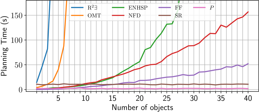
We also considered the LineExchange domain, which is a generalization of the domain in the Example. In this domain, $N=4$ robots are positioned in a line and need to exchange items while staying in their adjacent segments of length $D=2$. At the beginning, the first robot has $Q\in\mathbb{N}$ items and the goal is to transfer all the items to the last robot in the line. In Figure 1, we show how the planning time varies with $Q$: when $Q=1$, all the variables are essentially Boolean (since they have at most two possible values) and all the symbolic planners are outperformed by the search-based ones. As $Q$ increases, rolling-up the exchange actions becomes more important, and thus Patty and SpringRoll start to outperform the search-based planners. Patterns allow Patty to perform better than SpringRoll, while our $R^{2}\exists$ planner performs poorly because of the high number of assertions and variables produced.

Conclusions

We presented the pattern encoding which generalizes the state-of-the-art rolled-up and $R^{2}\exists$ encodings. We provided theoretical and experimental evidence of its benefits. We believe that our generalization provides a new starting point for the research in symbolic planning. Indeed, more research is needed to extend the ARPG construction for better patterns.

References

- Arxer and Scala (2023) Arxer, J. E.; and Scala, E. 2023. International Planning Competition 2023 - Numeric Tracks. https://ipc2023-numeric.github.io. Accessed: 2023-08-01.
- Barrett, Fontaine, and Tinelli (2016) Barrett, C.; Fontaine, P.; and Tinelli, C. 2016. The Satisfiability Modulo Theories Library (SMT-LIB). www.SMT-LIB.org. Accessed: 2024-01-06.
- Bofill, Espasa, and Villaret (2017) Bofill, M.; Espasa, J.; and Villaret, M. 2017. Relaxed Exists-Step Plans in Planning as SMT. In Sierra, C., ed., Proceedings of the Twenty-Sixth International Joint Conference on Artificial Intelligence, IJCAI 2017, Melbourne, Australia, August 19-25, 2017, 563–570. ijcai.org.
- Bonet and Geffner (2001) Bonet, B.; and Geffner, H. 2001. Planning as heuristic search. Artificial Intelligence, 129(1–2): 5–33.
- De Moura and Bjørner (2008) De Moura, L.; and Bjørner, N. 2008. Z3: An efficient SMT solver. In International conference on Tools and Algorithms for the Construction and Analysis of Systems, 337–340. Springer.
- Fox and Long (2003) Fox, M.; and Long, D. 2003. PDDL2.1: An Extension to PDDL for Expressing Temporal Planning Domains. Journal of Artificial Intelligence Research, 20: 61–124.
- Hoffmann (2003) Hoffmann, J. 2003. The Metric-FF Planning System: Translating“Ignoring Delete Lists”to Numeric State Variables. Journal of artificial intelligence research, 20: 291–341.
- Kautz and Selman (1992) Kautz, H. A.; and Selman, B. 1992. Planning as Satisfiability. In Neumann, B., ed., 10th European Conference on Artificial Intelligence, ECAI 92, Vienna, Austria, August 3-7, 1992. Proceedings, 359–363. John Wiley and Sons.
- Kuroiwa, Shleyfman, and Beck (2022) Kuroiwa, R.; Shleyfman, A.; and Beck, J. C. 2022. LM-Cut Heuristics for Optimal Linear Numeric Planning. In Proceedings of the International Conference on Automated Planning and Scheduling, volume 32, 203–212.
- Leofante et al. (2020) Leofante, F.; Giunchiglia, E.; Ábráham, E.; and Tacchella, A. 2020. Optimal Planning Modulo Theories. In Proceedings of the Twenty-Ninth International Joint Conference on Artificial Intelligence, 4128–4134. Yokohama, Japan: International Joint Conferences on Artificial Intelligence Organization. ISBN 978-0-9992411-6-5.
- McCarthy and Hayes (1969) McCarthy, J.; and Hayes, P. 1969. Some Philosophical Problems From the Standpoint of Artificial Intelligence. In Meltzer, B.; and Michie, D., eds., Machine Intelligence 4, 463–502. Edinburgh University Press.
- Rintanen, Heljanko, and Niemelä (2006) Rintanen, J.; Heljanko, K.; and Niemelä, I. 2006. Planning as satisfiability: parallel plans and algorithms for plan search. Artif. Intell., 170(12-13): 1031–1080.
- Scala, Haslum, and Thiebaux (2016) Scala, E.; Haslum, P.; and Thiebaux, S. 2016. Heuristics for Numeric Planning via Subgoaling. In Proceedings of the Twenty-Fifth International Joint Conference on Artificial Intelligence (IJCAI-16).
- Scala et al. (2016a) Scala, E.; Haslum, P.; Thiebaux, S.; and Ramirez, M. 2016a. Interval-Based Relaxation for General Numeric Planning. In Proceedings of the Twenty-second European Conference on Artificial Intelligence, 655–663.
- Scala et al. (2016b) Scala, E.; Ramirez, M.; Haslum, P.; and Thiebaux, S. 2016b. Numeric Planning with Disjunctive Global Constraints via SMT. Proceedings of the International Conference on Automated Planning and Scheduling, 26: 276–284.
- Scala et al. (2020) Scala, E.; Saetti, A.; Serina, I.; and Gerevini, A. E. 2020. Search-guidance mechanisms for numeric planning through subgoaling relaxation. In Proceedings of the International Conference on Automated Planning and Scheduling, volume 30, 226–234.