Toward fluid radiofrequency ablation of cardiac tissue: modeling, analysis and simulations

Abstract

This paper deals with the modeling, mathematical analysis and numerical simulations of a new model of nonlinear radiofrequency ablation of cardiac tissue. The model consists of a coupled thermistor and the incompressible Navier-Stokes equations that describe the evolution of temperature, velocity, and additional potential in cardiac tissue. Based on Schauder’s fixed-point theory, we establish the global existence of the solution in two- and three-dimensional space. Moreover, we prove the uniqueness of the solution under some additional conditions on the data and the solution. Finally, we discuss some numerical results for the proposed model using the finite element method.

1 Introduction

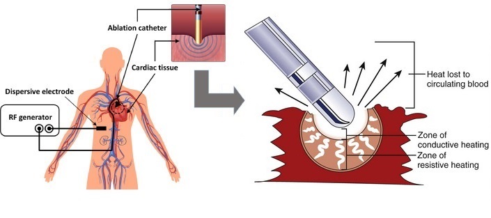
In recent years, radiofrequency ablation (RFA) techniques have been applied in various medical fields, for example in the elimination of cardiac arrhythmia, where the objective is to eliminate the tissue responsible for this disease or the destruction of tumors. During this procedure, catheters are directed into the heart to map its electrical activity and locate diseased areas, which are then removed through an ablation catheter, see Figure 2.

Figure 1: Radiofrequency ablation procedure in cardiac tissue .

For this reason, the desire to provide fast and low-cost essential information on the electrical and thermal behavior of ablation has motivated several theoretical and numerical studies to develop new techniques or to improve those currently used.

As is known, RFA models are usually described by a thermistor problem presented as a coupled system of nonlinear PDEs. These are the heat equation with Joule heating as the source and the current conservation equation with temperature-dependent electrical conductivity. In this context, many works in the literature deal with the precise modeling of the electrical and thermal characteristics of biological tissues, not only those that depend on temperature but also on time, i.e. to quantify the relationships between the characteristic values and the thermal damage function[3]. We refer the interested reader to  [16] for more details on modeling the study of radiofrequency ablation techniques. The aforementioned reference presents important issues involved in this methodology, including experimental validation, current limitations, especially those related to the lack of precise characterization of biological tissues, and suggestions and future perspectives of this field. For example, the application of saline infusion requires the derivation of a suitable model to follow the behavior of the tissue during the simultaneous application of RF energy and the cooling effect. It is worth mentioning that the author in [38] develops realistic modeling for large and medium blood vessels. While model derivation and fluid mechanics studies of blood flow, for example, in the carotid arteries, basilar trunk, and circle of Willis, are the subject of numerous contributions, see [22, 39] and references therein.

In this context, our paper deals with the mathematical analysis and numerical simulations of an RFA fluid model by coupling the thermistor model with the incompressible Navier-Stokes system. Our model takes into account the phenomena of viscous energy dissipation and electric field. Now, let’s present the mathematical formulation of the model below, which we will discuss in the next sections.

$$\left\{\begin{array}[]{rclll}\boldsymbol{v}_{t}+\nabla\cdot(\boldsymbol{v}\otimes\boldsymbol{v})-\nabla\cdot(\nu(\theta)\mathbb{D}(\boldsymbol{v}))+\nabla P&=&\boldsymbol{F}(\theta),&\text{ in }&\Omega_{T},\\ \nabla\cdot\boldsymbol{v}&=&0,&\text{ in }&\Omega_{T}\\ \boldsymbol{v}&=&\mathbf{0},&\text{ on }&\Sigma_{D},\\ -\mathbb{S}(\boldsymbol{v},P)\boldsymbol{n}&=&\mathbf{0},&\text{ on }&\Sigma_{N},\\ \boldsymbol{v}(\boldsymbol{x},0)&=&\boldsymbol{v}_{0},&\text{ on }&\Omega,\\ \theta_{t}-\nabla\cdot(\eta(\theta)k\nabla\theta)+\boldsymbol{v}\cdot\nabla\theta-\nu(\theta)\mathbb{D}(\boldsymbol{v}):\mathbb{D}(\boldsymbol{v})-(\sigma(\theta)\varrho\nabla\varphi)\cdot\nabla\varphi&=&0,&\text{ in }&\Omega_{T},\\ (\eta(\theta)k\nabla\theta)\cdot\boldsymbol{n}+\alpha\theta&=&\alpha\theta_{l},&\text{ on }&\Sigma,\\ \theta(x,0)&=&\theta_{0},&\text{ in }&\Omega,\\ -\operatorname{div}(\sigma(\theta)\varrho\nabla\varphi)&=&0,&\text{ in }&\Omega_{T},\\ (\sigma(\theta)\varrho\nabla\varphi)\cdot\boldsymbol{n}&=&g,&\text{ on }&\Sigma_{N},\\ \varphi&=&0,&\text{ on }&\Sigma_{D},\end{array}\right.$$ (1)

where $\Omega\subset\mathbb{R}^{d}$, $d=2,3$ is a bounded domain with a $C^{1,1}$ boundary $\partial\Omega=\Gamma$. We suppose that $\Gamma_{D}$ and $\Gamma_{N}$ are closed disjoint $(d-1)$-dimensional manifolds of class $C^{1,1}$ such that $\Gamma=\Gamma_{D}\cup\Gamma_{N}$ where $\Gamma_{D}$ represents solid surfaces and $\Gamma_{N}$ denotes the artificial part of the boundary $\partial\Omega$. Let $T\in(0,\infty)$ be fixed throughout the paper, $\Omega_{T}=\Omega\times(0,T)$, $\Sigma=\partial\Omega\times(0,T)$, $\Sigma_{N}=\Gamma_{N}\times(0,T)$ and $\Sigma_{D}=\Gamma_{D}\times(0,T)$. In model (1), $\boldsymbol{v}$ is the flow velocity, $P$ is the pressure scaled by the density $\rho$ and the parameter $\nu$ is the kinematic viscosity. Moreover, $\mathbb{D}(\boldsymbol{v})=\frac{1}{2}\left(\nabla\boldsymbol{v}+\nabla\boldsymbol{v}^{T}\right)$ is the strain rate tensor, $\mathbb{S}(\boldsymbol{v},P)=\nu(\theta)\mathbb{D}(\boldsymbol{v})-PI$ is the Cauchy stress tensor, $\boldsymbol{F}$ is a right hand side and $(\eta(\cdot)k)$ represents the heat conductivity. While $k$ is a prescribed function, $\eta$ is allowed to depend on the temperature $\theta$ and $\alpha$ is the heat transfer coefficient regulating the convective heat flux through the boundary $\partial\Omega$. The functions $\theta_{l}$ and $\theta_{0}$ are given boundary and initial data, respectively. The function $\sigma(\cdot)\varrho$ represents the electric conductivity, $\varrho$ is a given prescribed function, $g$ stands for a current which is induced via the boundary part $\Gamma_{N}$, and $\sigma$ is allowed to depend on the temperature $\theta$. At the inflow, we impose a constant velocity $\boldsymbol{v}$, since blood comes from the microcirculation, modeled by a quasi-steady/steady Stokes flow. At the wall, we impose $\boldsymbol{v}=0$, since intracranial veins are constrained between a nearly incompressible brain and the rigid skull and at the outflow, we impose in a first approximation $\mathbb{S}(\boldsymbol{v},p)n=0$, called do-nothing classical approach.

We mention that systems reduced to heat-potential coupled models (thermistors) or to Navier-Stokes-heat coupled models are widely discussed in the literature. Let us quote here some references for the theoretical analysis of the first coupling, that is to say, the models of thermal potential. Time-dependent thermistor equations in particular have been widely studied as described in  [18, 41, 6, 33]. Among these works: the existence of the solution using the maximum principle and the fixed point argument in [6], the existence of the weak solution for an arbitrarily large time interval using the Faedo-Galerkin method in [18]. Recently, the existence and uniqueness of the solution for the thermistor problem without non-degenerate assumptions in [33]. For the special case where the thermal conductivity is constant, the authors in [41] proved the existence and uniqueness of the solution in three-dimensional space and its continuity $\alpha$-Hölder, it is possible to obtain greater regularity of the solution by making appropriate assumptions about the initial and boundary conditions. Moreover, this system has motivated other areas of applied mathematics, such as optimal control and inverse problems, namely the identification of the frequency factor and the energy of the thermal damage function for different types of tissues such as liver, breast, heart, etc., and the development of rapid numerical simulations to predict tissue temperature and thus provide simultaneous guidance during an intervention [29, 40]. We also cite the two interesting works [35, 36] where the well-posed character is shown and the optimality conditions are derived by considering the parameter $g$ as a boundary check.

The theoretical studies of the second coupling have been the subject of several works, we refer the reader to  [15, 13, 12, 19] and the references contained therein. Among these works, the authors of [19] studied the case where viscosity and thermal conductivity are nonlinear and temperature dependent. In the aforementioned paper, the authors derived the existence of solutions, without restriction on the data, by Brouwer’s fixed point theorem. On the other hand, in [20] the authors have studied the existence and the uniqueness of the solution using the Brouwer fixed point, the Faedo-Galerkin method, and some compactness results for a model variant of this coupling namely, the globally modified Navier-Stokes problem coupled to the heat equation. The authors studied the stability of the discrete solution in time using the energy approach. We mention the paper [15] where the authors considered the external force in the heat equation containing an energy dissipation term. Moreover, they proved the existence of the solution for three-dimensional space using Galerkin’s method and Schauder’s fixed point theorem.

From a computational point of view, there are very few computational analyses for the general case. We mention the work in [5] where the semi-discretization in space by the finite volume method has been proposed to solve the thermistor problem. The $L^{2}$-norm and $H^{1}$-norm error estimates have been obtained for the piecewise linear approximation, a linearized $\theta$-Galerkin finite element method is proposed to solve the coupled system, and optimal error estimates are derived in different cases, including the standard Crank-Nicolson and shifted Crank-Nicolson schemes in [34]. Numerical methods and analysis for the thermistor system for special conductivities, namely, for the linear and the exponential choices, have been investigated by many authors [18, 31, 32, 4, 21]. For a constant thermic conductivity in two-dimensional space, the optimal $L^{2}$-norm error estimate of a mixed finite element method with a linearized semi-implicit Euler scheme was obtained in [4] under a weak time-step condition. The error analysis for the three-dimensional space is given in [21] using a linearized semi-implicit Euler scheme with a linear Galerkin finite element method. An optimal $L^{2}$-norm error estimate was obtained under specific conditions on the step size discretization. For the $d$-dimensional space $(d=2,3)$, the authors in [32] proved the time-step condition of commonly-used linearized semi-implicit schemes for the time-dependent nonlinear Joule heating equations with Galerkin finite element approximations and optimal error estimates of a Crank-Nicolson Galerkin method for the nonlinear thermistor equations [31] and backward differential formula type similarly schemes approximations [23]. Different methods have been considered to approximate the Navier-Stokes equations coupled to the heat equation [19, 37, 7]. The authors in [19] presented a convergence analysis for an iterative scheme based on the so-called coupled prediction scheme. Finally, the virtual element discretization of the Navier-Stokes equations coupled to the heat equation where the viscosity depends on temperature was studied in [7]. The authors showed that it is well-posed and proved optimal error estimates for this discretization.

In the present study, we analyze the proposed model (1) in a two- and three-dimensional space by placing it in an equivalent variational formulation. The global existence and uniqueness of the solutions are derived without restriction on the data by Schauder’s fixed-point theory. In addition, the variational formulation is discretized by the finite element method in a domain with fairly realistic geometry. Subsequently, some numerical experiments of the proposed model are provided. Besides the theoretical and numerical complexity of the proposed model, discussed later, we recall that the physical and biological properties of the tissues present obstacles. Indeed, all model variables must fall within specific ranges and the results of numerical experiments must be consistent with these criteria. For example, the electrical and thermal conductivities show significantly variable values due to phenomena associated with the high temperatures reached during RFA, such as the vaporization of water at temperatures close to $100\,^{\circ}C$ and the ensuing sudden increase in impedance, which hampers the delivery of RF power, thus limiting the size of the lesion. Additionally, the presence of the energy dissipation term due to viscosities $\displaystyle\nu(\theta)\mathbb{D}(\boldsymbol{v}):\mathbb{D}(\boldsymbol{v})$ and $\sigma(\theta)\varrho\nabla\varphi\cdot\nabla\varphi$ is one of the difficulties in studying such models. On the contrary, in the well-known Boussinesq system, when this term is ignored, the study is generally more intuitive. Compared to [15], our contribution concerned three parts, namely modeling, well-posedness and numerical simulations. Indeed, our proposed model (1) is improved by taking into account the potential effect. Thus, it contains coupling terms $(\sigma(\theta)\varrho\nabla\varphi)\cdot\nabla\varphi$ and $-\operatorname{div}(\sigma(\theta)\varrho\nabla\varphi)$ . Thus, from a modeling point of view, this is more close to reality. In addition, in this paper we prove the existence and also uniqueness of the solutions in two and three-dimensional spaces. Furthermore, this paper provides the numerical simulations.

The rest of this paper is organized as follows. In the next section, we introduce the basic notations and some appropriate functional spaces. Then, we formulate the problem according to a variational framework and introduce one of the main results of our work. In Section 3, we investigate the existence, uniqueness, and energy estimates of solutions to linearized (decoupled) initial boundary value problems for the Navier-Stokes, electric potential, and heat with non-smooth coefficients. Moreover, we prove the existence item of the main result using Schauder’s fixed point. To complete the proof of the main result, we prove the uniqueness of the solution. Finally, we discuss in Section 4 some numerical simulations in two-dimensional space by the finite element method.

2 Mathematical frameworks and variational formulation

We consider $p$, $q$, $r$, $p^{\prime}\in[1,\infty]$, where $p^{\prime}$ denotes the conjugate exponent to $p>1$ namely $1/p+1/p^{\prime}=1$. For an arbitrary $r\in[1,+\infty]$, $L^{r}(\Omega)$ is the usual Lebesgue space equipped with the norm $\|\cdot\|_{L^{r}(\Omega)}$, and $W^{m,r}(\Omega)$, $m\geq 0$ $(m$ need not to be an integer$)$, denotes the usual Sobolev space with the norm $\|\cdot\|_{W^{m,r}(\Omega)}$. By $C(0,T;E)$ we denote the space of all abstract functions $\psi$ such that $\psi$: $(0,T)\longmapsto E$ is continuous, where $E$ is a Banach space. Further, we denote by $W^{-m,p}(\Omega)$ the dual space of $W^{m,p^{\prime}}(\Omega)$. For simplicity reason, we denote shortly $\mathbf{W}^{m,p}(\Omega)\equiv W^{m,p}(\Omega)^{d}$, $\mathbf{L}^{r}(\Omega)\equiv L^{r}(\Omega)^{d}$, $\lambda(\cdot):=\sigma(\cdot)\varrho$ and $\gamma(\cdot):=\eta(\cdot)k$.

For the mathematical analysis of our model (1), we use the following embedding results (see [1, Theorem 7.58] and  [30])

$$\begin{array}[]{llll}W^{m,p}(\Omega)&\hookrightarrow L^{q}(\Omega),&\|\phi\|_{L^{q}{(\Omega)}}\leq c\|\phi\|_{W^{m,p}(\Omega)},&p\leq q<\infty,mp=d,\\ W^{m,p}(\Omega)&\hookrightarrow L^{q}(\Omega),&\|\phi\|_{L^{q}(\Omega)}\leq c\|\phi\|_{W^{m,p}(\Omega)},&p\leq q\leq dp/(d-mp),mp<d,\\ W^{m,p}(\Omega)&\hookrightarrow L^{\infty}(\Omega),&\|\phi\|_{L^{\infty}(\Omega)}\leq c\|\phi\|_{W^{m,p}(\Omega)},&mp>d,\end{array}$$ (2)

for every $\phi\in W^{m,p}(\Omega)$. Further, there exists a continuous operator $\mathfrak{R}_{0}:W^{m,p}(\Omega)\rightarrow L^{q}(\partial\Omega)$ such that

$$\|\mathfrak{R}_{0}(\phi)\|_{L^{q}(\partial\Omega)}\leq c\|\phi\|_{W^{m,p}(\Omega)}\;\forall\phi\in W^{m,p}(\Omega)\hbox{ with }\left\{\begin{array}[]{ll}1\leq mp<d,&q=\frac{dp-p}{d-mp},\\ p\geq\max\{1,d/m\},&q\in[1,\infty).\end{array}\right.$$ (3)

For $s$ be real number such that $s\leq m+1,s-1/p=k+\sigma$, where $k\geq 1$ is an integer and $0<\sigma<1$, the following mapping $\mathfrak{R}_{1}$ is continuous

$$\mathfrak{R}_{1}:W^{s,p}(\Omega) \rightarrow W^{s-1-1/p,p}(\Gamma),$$ (4)

$$\varphi \mapsto\frac{\partial\varphi}{\partial n}{\mid_{\Gamma}}.$$

Let consider the following spaces

$$\begin{array}[]{ll}\mathcal{E}_{\boldsymbol{v}}:=&\left\{\boldsymbol{v}\in\boldsymbol{C}^{\infty}(\overline{\Omega});\text{}\operatorname{div}\boldsymbol{v}=0,\text{}\operatorname{supp}\boldsymbol{v}\cap\Gamma_{D}=\emptyset\right\}\text{, }\\ \mathcal{E}_{\varphi}:=&\left\{\varphi\in C^{\infty}(\overline{\Omega});\text{}\operatorname{supp}\varphi\cap\Gamma_{D}=\emptyset\right\}\text{, }\\ \mathcal{E}_{\theta}:=&\left\{\theta\in C^{\infty}(\overline{\Omega});\text{}\operatorname{supp}\theta\text{ is compact }\right\},\end{array}$$

and let $\mathbf{V}_{\boldsymbol{v}}^{m,p}$ be the closure of $\mathcal{E}_{\boldsymbol{v}}$ in the norm of $\mathbf{W}^{m,p}(\Omega)$, $m\geq 0$ and $1\leq p\leq\infty$. Similarly, let $V_{\varphi}^{m,p}$ and $V_{\theta}^{m,p}$ are the closures of $\mathcal{E}_{\varphi}$ and $\mathcal{E}_{\theta}$ in the norm of $W^{m,p}(\Omega)$. Then $V_{\theta}^{m,p}$, $V_{\varphi}^{m,p}$ and $\mathbf{V}_{\boldsymbol{v}}^{m,p}$ are Banach spaces with the norms of the spaces $W^{m,p}(\Omega)$ and $\mathbf{W}^{m,p}(\Omega)$, respectively. Note that the Banach space $V_{\varphi}$ is defined by $V_{\varphi}=\{\phi\in{V}_{\varphi}^{1,2},\nabla\phi\in\mathbf{L}^{4}(\Omega)\}$ equipped with the norm

$${\|{\phi}\|}_{V_{\varphi}}:=\|\phi\|_{V_{\varphi}^{1,2}}+\|\nabla{\phi}\|_{\mathbf{L}^{4}(\Omega)}.$$

Finally, for $m>0,\mathbf{V}_{v}^{-m,p}$ denotes the dual space of $\mathbf{V}_{v}^{m,p^{\prime}}$ normed by

$${\|\mathbf{v}\|}_{\mathbf{V}_{v}^{-m,p}}=\sup_{\mathbf{0}\neq\mathbf{w}\in\mathbf{V}_{v}^{m,p^{\prime}}}\frac{|\langle\boldsymbol{v},\mathbf{w}\rangle|}{\|\mathbf{w}\|_{\mathbf{W}^{m,p^{\prime}}}},$$

where $\langle\cdot,\cdot\rangle$ denotes the duality pairing.

If the functions $\boldsymbol{v}$, $\boldsymbol{w}$, $\boldsymbol{z}$, $\theta$, $\phi$, $\varphi$, $\chi$ and $\psi$ are sufficiently smooth so that the following integrals make sense, we also introduce the following notations:

$$(\boldsymbol{v},\boldsymbol{w}) =\int_{\Omega}\boldsymbol{v}\cdot\boldsymbol{w}\mathrm{~{}d}x,\qquad (\theta,\psi)_{\Gamma} =\int_{\Gamma}\theta\psi\mathrm{d}\Gamma,$$

$$a_{u}(\theta;\boldsymbol{v},\boldsymbol{w}) =\int_{\Omega}\nu(\theta)\mathbb{D}(\boldsymbol{v}):\mathbb{D}(\boldsymbol{w})\mathrm{~{}d}x,\qquad \tilde{a}_{u}(\boldsymbol{v},\boldsymbol{w}) =\int_{\Omega}\mathbb{D}(\boldsymbol{v}):\mathbb{D}(\boldsymbol{w})\mathrm{~{}d}x,$$

$$a_{\theta}(\phi;\theta,\psi) =\int_{\Omega}\gamma(\phi)\nabla\theta\cdot\nabla\psi\mathrm{~{}d}x,\qquad \tilde{a}_{\theta}(\theta,\varphi) =\int_{\Omega}\nabla\theta\cdot\nabla\varphi\mathrm{~{}d}x,$$

$$c_{\varphi}(\phi,\varphi,\psi) =\int_{\Omega}\lambda(\phi)\nabla\varphi\cdot\nabla\varphi\psi\mathrm{~{}d}x,\qquad a_{\varphi}(\phi,\varphi,\chi) =\int_{\Omega}\lambda(\phi)\nabla\varphi\cdot\nabla\chi\mathrm{~{}d}x,$$

$$d(\boldsymbol{v},\theta,\psi) =\int_{\Omega}(\boldsymbol{v}\cdot\nabla\theta)\psi\mathrm{~{}d}x,\qquad e(\theta;\boldsymbol{v},\boldsymbol{w},\psi) =\int_{\Omega}\nu(\theta)\mathbb{D}(\boldsymbol{v}):\mathbb{D}(\boldsymbol{w})\psi\mathrm{~{}d}x,$$

$$b(\boldsymbol{v},\boldsymbol{w},\boldsymbol{z}) =\int_{\Gamma_{N}}(\boldsymbol{v}\otimes\boldsymbol{w}):(\boldsymbol{n}\otimes\boldsymbol{z})\mathrm{d}\Gamma-\int_{\Omega}(\boldsymbol{v}\otimes\boldsymbol{w}):\mathbb{D}(\boldsymbol{z})\mathrm{~{}d}x.$$

To formulate model (1) in a variational sense and then state the main result of the paper, the following smoothness property is needed.

Lemma 2.1 (cf [15])

Let $\boldsymbol{\mathcal{U}}$ a Banach space defined by

$$\boldsymbol{\mathcal{U}}:=\left\{\boldsymbol{z}\mid\boldsymbol{z}\in L^{\infty}\left(0,T;\mathbf{V}_{\boldsymbol{v}}^{0,4}\right)\cap L^{4}\left(0,T;\mathbf{V}_{\boldsymbol{v}}^{1,4}\right)\right\}\text{, }$$

equipped with the norm

$${\|\boldsymbol{z}\|}_{\boldsymbol{\mathcal{U}}}:=\|\boldsymbol{z}\|_{L^{\infty}\left(0,T;\mathbf{V}_{\boldsymbol{v}}^{0,4}\right)}+\|\boldsymbol{z}\|_{L^{4}\left(0,T;\mathbf{V}_{\boldsymbol{v}}^{1,4}\right)}.$$

Then

$$\boldsymbol{\mathcal{U}}\hookrightarrow L^{64/7}\left(0,T;\mathbf{W}^{7/16,4}\right).$$ (5)

In addition, for all $(\boldsymbol{v},\boldsymbol{w})\in\boldsymbol{\mathcal{U}}^{2}$, $b(\boldsymbol{v},\boldsymbol{w},\cdot)\in L^{4}\left(0,T;\mathbf{V}_{\boldsymbol{v}}^{-1,4}\right)$ and there exists some positive constant $C_{b},$ independent of $T,$ such that

$$\|b(\boldsymbol{v},\boldsymbol{w},\cdot)\|_{L^{4}\left(0,T;\mathbf{V}_{\boldsymbol{v}}^{-1,4}\right)}\leq C_{b}T^{1/32}{\|\boldsymbol{v}\|}_{\boldsymbol{\mathcal{U}}}{\|\boldsymbol{w}\|}_{\boldsymbol{\mathcal{U}}}\text{.}$$ (6)

We will solve the system (1) with the followings assumptions:

• The functions $\boldsymbol{F}=\boldsymbol{F}(\cdot)$, $\nu=\nu(\cdot)$, $\lambda=\lambda(\cdot)$ and $\gamma=\gamma(\cdot)$ being positives, bounded and continuous for the temperature. Without any further reference, we assume

  $$0\leq F_{i}(s)\leq C_{F}<+\infty\qquad \forall s\in\mathbb{R},i=1,...,d,$$ (7)

  $$0<\nu_{1}\leq\nu(s)\leq\nu_{2}<+\infty\qquad \forall s\in\mathbb{R},$$ (8)

  $$0<\lambda_{1}\leq\lambda(s)\leq\lambda_{2}<+\infty\qquad \forall s\in\mathbb{R},$$ (9)

  $$0<\gamma_{1}\leq\gamma(s)\leq\gamma_{2}<+\infty\qquad \forall s\in\mathbb{R},$$ (10)

  where $C_{F}$, $\nu_{1}$, $\nu_{2}$, $\lambda_{1}$, $\lambda_{2}$, $\gamma_{1}$ and $\gamma_{2}$ are positive constants.

• The initials data $\boldsymbol{v}_{0}\in\mathbf{V}_{\boldsymbol{v}}^{1/2,4}$, $\theta_{0}\in L^{2}$.

• The other assumptions on the data are,

  $$\mathbf{F}\in L^{4}\left(0,T;\mathbf{V}_{\boldsymbol{v}}^{-1,4}\right),\text{ }\theta_{l}\in L^{2}\left(0,T;V_{\theta}^{1,2}\right)\cap L^{2}\left(0,T;V_{\theta}^{-1,2}\right)\text{ and }\,g\in L^{4}\left(0,T;W^{-1/2,2}(\Gamma)\right).$$ (11)

• There exists a constant $C_{S}$ (to be specified later, cf (25)) such that

  $$C_{S}\left(\nu_{2}-\nu_{1}\right)<1.$$ (12)

• There exists $\beta\in\left(0,1/2\left(1-C_{S}\left(\nu_{2}-\nu_{1}\right)\right)\right)$ such that (recall that the constants $C_{F}$ and $C_{S}$ are defined in (7) and (12), respectively)

  $$C_{S}C_{E}C_{F}C_{d}(\Omega,T)+C_{S}\left\|\boldsymbol{v}_{0}\right\|_{\mathbf{V}_{\boldsymbol{v}}^{1/2,4}}\leq\frac{\beta^{2}}{C_{S}C_{b}T^{1/32}},$$ (13)

where $C_{d}(\Omega,T)=T^{1/4}d^{1/2}\operatorname{meas}(\Omega)^{1/4}$, $C_{E}$ is the constant of the embedding $\mathbf{W}^{1,4/3}\hookrightarrow~{}\mathbf{L}^{4/3}$ and $C_{b}$ is a given constant from $(\ref{cstb})$.

We will utilize the following notion of weak solution for our model (1).

Definition 2.1

(Weak solution). A triplet $(\boldsymbol{v},\theta,\varphi)$ is called variational solution of the problem (1) if $\boldsymbol{v}_{0}\in\mathbf{V}_{\boldsymbol{v}}^{1/2,4}$, $\theta_{0}\in L^{2}$, $\boldsymbol{v}\in\boldsymbol{\mathcal{U}}$, $\boldsymbol{v}_{t}\in L^{4}\left(0,T;\mathbf{V}_{\boldsymbol{v}}^{-1,4}\right)$, $\theta\in L^{2}\left(0,T;V_{\theta}^{1,2}\right)$, $\theta_{t}\in L^{2}\left(0,T;V_{\theta}^{-1,2}\right)$ and $\varphi\in L^{4}\left(0,T;V_{\varphi}\right)$, and the following variational formulations

$$\left\langle\boldsymbol{v}_{t},\boldsymbol{w}\right\rangle+a_{u}(\theta;\boldsymbol{v},\boldsymbol{w})+b(\boldsymbol{v},\boldsymbol{v},\boldsymbol{w}) = \left\langle\boldsymbol{F}(\theta),\boldsymbol{w}\right\rangle,$$ (14)

$$\left\langle\theta_{t},\psi\right\rangle+a_{\theta}(\theta;\theta,\psi)+d(\boldsymbol{v},\theta,\psi)+\alpha(\theta,\psi)_{\Gamma}-e(\theta;\boldsymbol{v},\boldsymbol{v},\psi)-c_{\varphi}(\theta,\varphi,\psi) = \alpha(\theta_{l},\psi)_{\Gamma,}$$ (15)

$$a_{\varphi}(\theta;\varphi,\chi) = {(g,\chi)}_{\Gamma_{N}},$$ (16)

hold for every $\left(\boldsymbol{w},\psi,\chi\right)\in\mathbf{V}_{\boldsymbol{v}}^{1,4/3}\times V_{\theta}^{1,2}\times V_{\varphi}^{1,2}$ and for almost every $t\in(0,T)$ and

$$\boldsymbol{v}(\boldsymbol{x},0) =\boldsymbol{v}_{0}(\boldsymbol{x}) \text{ in }\Omega,$$ (17)

$$\theta(\boldsymbol{x},0) =\theta_{0}(\boldsymbol{x}) \text{ in }\Omega.$$ (18)

Our main result is

Theorem 2.1

(Well-posedness).

1. Existence: Assume that assumptions (A1), (A2), (A3), (A4), and (A5) hold. Then System (14)-(16) has a weak solution $\left(\boldsymbol{v},\theta,\varphi\right)\in\boldsymbol{\mathcal{U}}\times C(0,T;V_{\theta}^{1,2})\times L^{4}\left(0,T;V_{\varphi}\right)$ in the sense of Definition 2.1.

2. Uniqueness: Let, in addition to assumptions (A1)-(A5) $\mathbf{F}$, $\nu$, $\lambda$ and $\gamma$ are Lipschitz continuous, i.e

   $$\left|\mathbf{F}\left(z_{1}\right)-\mathbf{F}\left(z_{2}\right)\right| \leq L_{\mathbf{F}}\left|z_{1}-z_{2}\right|\quad\forall z_{1},z_{2}\in\mathbb{R}\left(L_{\mathbf{F}}=\text{ const }>0\right),$$ (19)

   $$\left|\nu\left(z_{1}\right)-\nu\left(z_{2}\right)\right| \leq L_{\nu}\left|z_{1}-z_{2}\right|\quad\forall z_{1},z_{2}\in\mathbb{R}\left(L_{\nu}=\text{ const }>0\right),$$

   $$\left|\lambda\left(z_{1}\right)-\lambda\left(z_{2}\right)\right| \leq L_{\lambda}\left|z_{1}-z_{2}\right|\quad\forall z_{1},z_{2}\in\mathbb{R}\left(L_{\lambda}=\text{ const }>0\right),$$

   $$\left|\gamma\left(z_{1}\right)-\gamma\left(z_{2}\right)\right| \leq L_{\gamma}\left|z_{1}-z_{2}\right|\quad\forall z_{1},z_{2}\in\mathbb{R}\left(L_{\gamma}=\text{ const }>0\right),$$

   and if $\nabla\theta\in L^{s}(0,T;W^{1,2}(\Omega))$, $\boldsymbol{u}\in L^{s}(0,T;\boldsymbol{W}^{1,2}(\Omega))$ and $\varphi\in L^{s}(0,T;W^{1,2}(\Omega))$ where $s=\frac{8}{4-d}$, then the weak solution of problem $(\ref{eqvar1})-(\ref{eqvar3})$ is unique.

3 Well-posedness analysis

This section deals with the proof of Theorem 2.1. Let us briefly describe the rough idea of the proof. For given temperature, say $\overline{\theta}$, in the kinematic viscosity $\nu$ and the last term in the first line in $(\ref{DecoupledNS})$ i.e the right-hand side $\boldsymbol{F}$, we find $\boldsymbol{v}$, the solution of the decoupled Navier-Stokes equations $(\ref{DecoupledNS})$ via the Banach contraction principle. Further, we find $\varphi$, the solution of decoupled potential equation (21) using Lax-Milgram’s method with the electrical conductivity is also depend of $\overline{\theta}$. Now with $\boldsymbol{v}$ and $\varphi$ in hand, we find $\theta$, the solution of the linearized heat equation with the second member is the some of two terms, the dissipative energy and electric field. Finally, we show that the map $\overline{\theta}\rightarrow\theta$ is completely continuous and maps some ball independent of the choice $\overline{\theta}$ into itself. Hence, the existence of at least one solution follows from the Schauder’s point fixe theorem. In Section 3.5, the uniqueness of the solution is established under the assumptions of Lipschitz continuity of the data (see equation $(\ref{lipchtz})$) and higher regularity of $\theta$.

3.1 Well-posedness of decoupled Navier-Stokes system and decoupled potential equation

For an arbitrary fixed $\overline{\theta}\in L^{2}\left(0,T;L^{2}\right)$, we consider the decoupled Navier-Stokes problem

$$\left\{\begin{array}[]{rclll}\boldsymbol{v}_{t}-\nabla\cdot(\nu(\overline{\theta})\mathbb{D}(\boldsymbol{v}))+\nabla\cdot(\boldsymbol{v}\otimes\boldsymbol{v})+\nabla P&=&\boldsymbol{F}(\overline{\theta}),&\hbox{ in }\Omega_{T}\\ \nabla\cdot\boldsymbol{v}&=&0&\hbox{ in }\Omega_{T},\\ \boldsymbol{v}&=&0&\hbox{ on }\Sigma_{D},\\ -P\boldsymbol{n}+\nu(\overline{\theta})\mathbb{D}(\boldsymbol{v})\boldsymbol{n}&=&\mathbf{0}&\hbox{ on }\Sigma_{N},\\ \boldsymbol{v}(\boldsymbol{x},0)&=&\boldsymbol{v}_{0}(\boldsymbol{x})&\,\hbox{ in }\hbox{ }\Omega.\end{array}\right.$$ (20)

and the decoupled potential problem

$$\left\{\begin{array}[]{rclll}-\operatorname{div}(\lambda(\overline{\theta})\nabla\varphi)&=&0&\hbox{ in }&\Omega_{T},\\ (\lambda(\overline{\theta})\nabla\varphi)\cdot\boldsymbol{n}&=&g&\hbox{ on }&\Sigma_{N},\\ \varphi&=&0&\hbox{ on }&\Sigma_{D}.\end{array}\right.$$ (21)

Remark 3.1

In [15] the authors proved the existence and the uniqueness of the solution to the decoupled Navier-Stokes problem (20) such that $\boldsymbol{v}\in\boldsymbol{\mathcal{U}}$ with $\boldsymbol{v}_{t}\in L^{4}\left(0,T;\boldsymbol{V}_{\boldsymbol{v}}^{-1,4}\right)$ for $d=3$. For $d=2$, the new paper [14] prescribed an additional condition of the viscosity on $\Gamma_{N}$ i.e the homogeneous Neumann boundary condition and consider the small data. The authors shown that the solution satisfies $\boldsymbol{v}\in L^{\infty}\left(0,T;\boldsymbol{V}_{\boldsymbol{v}}^{s-1,2}\right)\cap L^{2}\left(0,T;\boldsymbol{V}_{\boldsymbol{v}}^{s,2}\right)$ with $\boldsymbol{v}_{t}\in L^{2}\left(0,T;\boldsymbol{V}_{\boldsymbol{v}}^{s-2,2}\right)$ for $s>1$.

We define the following nonlinear mapping

$$\begin{array}[]{lclll}\mathcal{S}_{1}:&L^{2}\left(0,T;L^{2}\right)&\rightarrow&\boldsymbol{\mathcal{U}}\times L^{4}\left(0,T;V_{\varphi}\right)\\ &\overline{\theta}&\mapsto&(\boldsymbol{v},\varphi)&\end{array}$$ (24)

where $\boldsymbol{v}$ is solution of (20) and $\varphi$ is solution of (21). The above mapping is well defined as we will show in the following (cf Theorem 3.2 and Theorem 3.5 ). In order to prove $\boldsymbol{v}$ is solution of (20), we need the following lemma.

Lemma 3.1 (The decoupled Stokes problem)

Let $\boldsymbol{f}\in L^{4}\left(0,T;\mathbf{V}_{\boldsymbol{v}}^{-1,4}\right)$ and $\boldsymbol{v}_{0}\in\mathbf{V}_{\boldsymbol{v}}^{1/2,4}$. Then there exists a unique function $\boldsymbol{v}\in\boldsymbol{\mathcal{U}}$ with $\boldsymbol{v}_{t}\in L^{4}\left(0,T;\boldsymbol{V}_{\boldsymbol{v}}^{-1,4}\right)$ satisfying

$$\left\langle\boldsymbol{v}_{t},\boldsymbol{w}\right\rangle+\tilde{a}_{u}\left(\nu_{2}\boldsymbol{v},\boldsymbol{w}\right)=\langle\boldsymbol{f},\boldsymbol{w}\rangle,$$

for all $\boldsymbol{w}\in\boldsymbol{V}_{\boldsymbol{v}}^{1,4/3}$ and almost every $t\in(0,T)$, $\boldsymbol{v}(\boldsymbol{.},0)=\boldsymbol{v}_{0}(\boldsymbol{.})\quad\hbox{ in }\Omega$. Moreover, $\boldsymbol{v}$ satisfying the following inequality

$${\|\boldsymbol{v}\|}_{\boldsymbol{\mathcal{U}}}\leq C_{S}\left(\|\boldsymbol{f}\|_{L^{4}\left(0,T;\mathbf{V}_{\boldsymbol{v}}^{-1,4}\right)}+\left\|\boldsymbol{v}_{0}\right\|_{\mathbf{V}_{\boldsymbol{v}}^{1/2,4}}\right),$$ (25)

where $C_{S}$ is a positive constant independent of $\boldsymbol{v}$, $\boldsymbol{f}$ and $\boldsymbol{v}_{0}$.

Proof 3.1.

We refer to [15, Theorem 4.1 and Corollary 4.2] for the proof.

The following theorem ensures the well-posedness of decoupled Navier-Stokes system $(\ref{DecoupledNS})$.

Theorem 3.2 (Well-posedness of System $(\ref{DecoupledNS})$).

Let $\overline{\theta}\in L^{2}\left(0,T;L^{2}\right)$ and $\boldsymbol{v}_{0}\in\mathbf{V}_{\boldsymbol{v}}^{1/2,4}$. Then there exists a unique function $\boldsymbol{v}\in\boldsymbol{\mathcal{U}}$ with $\boldsymbol{v}_{t}\in L^{4}\left(0,T;\mathbf{V}_{\boldsymbol{v}}^{-1,4}\right)$ such that

$$\left\{\begin{array}[]{rllll}\left\langle\boldsymbol{v}_{t},\boldsymbol{w}\right\rangle+a_{u}(\overline{\theta};\boldsymbol{v},\boldsymbol{w})+b(\boldsymbol{v},\boldsymbol{v},\boldsymbol{w})&=&\langle\boldsymbol{F}(\overline{\theta}),\boldsymbol{w}\rangle,&\forall\boldsymbol{w}\in\mathbf{V}_{\boldsymbol{v}}^{1,4/3}\hbox{ and a.e }t\in(0,T),\\ \boldsymbol{v}(\boldsymbol{x},0)&=&\boldsymbol{v}_{0}(\boldsymbol{x}),&\forall x\in\Omega.\end{array}\right.$$ (26)

Proof 3.3.

By Hölder inequality and the Sobolev embedding $(\ref{inject1})$, we infer

$$|(\boldsymbol{F}(\overline{\theta}),\boldsymbol{w})| \leq\|\boldsymbol{F}(\overline{\theta})\|_{\mathbf{L}^{4}}\|\boldsymbol{w}\|_{\boldsymbol{L}^{4/3}}$$

$$\leq C_{E}\|\boldsymbol{F}(\overline{\theta})\|_{\mathbf{L}^{4}}\|\boldsymbol{w}\|_{\boldsymbol{W}^{1,4/3}},$$

for every $\boldsymbol{w}\in\mathbf{W}^{1,4/3}$. Then,

$$\|\boldsymbol{F}(\overline{\theta})\|_{\boldsymbol{V_{u}}^{-1,4}} \leq C_{E}\left(\int_{\Omega}(|\boldsymbol{F}(\overline{\theta})|_{E})^{4}\mathrm{~{}d}x\right)^{1/4}$$

$$\leq C_{E}\left(\int_{\Omega}(d^{1/2}C_{F})^{4}\mathrm{~{}d}x\right)^{1/4}$$

$$\leq C_{E}C_{F}d^{1/2}\operatorname{meas}(\Omega)^{1/4},$$

where $|\cdot|_{E}$ denotes the Euclidean vector norm. Raising both sides and integrating over $(0,T)$ we get,

$$\|\boldsymbol{F}(\overline{\theta})\|_{L^{4}(0,T;\mathbf{V}_{\boldsymbol{v}}^{-1,4})} \leq C_{E}C_{F}C_{d}(\Omega,T).$$

Let $\overline{\boldsymbol{v}}\in\boldsymbol{\mathcal{U}}$. By Lemma 2.1 and Lemma 3.1, there exists the unique function $\boldsymbol{v}\in\boldsymbol{\mathcal{U}}$ with $\boldsymbol{v}_{t}\in L^{4}\left(0,T;\mathbf{V}_{\boldsymbol{v}}^{-1,4}\right)$ such that

$$\left\{\begin{array}[]{rclll}\left\langle\boldsymbol{v}_{t},\boldsymbol{w}\right\rangle+\tilde{a}_{u}\left(\nu_{2}\boldsymbol{v},\boldsymbol{w}\right)&=&(\boldsymbol{F}(\overline{\theta}),\boldsymbol{w})+\tilde{a}_{u}\left(\nu_{2}\overline{\boldsymbol{v}},\boldsymbol{w}\right)-a_{u}(\overline{\theta},\overline{\boldsymbol{v}},\boldsymbol{w})-b(\overline{\boldsymbol{v}},\overline{\boldsymbol{v}},\boldsymbol{w}),\\ \boldsymbol{v}(\boldsymbol{x},0)&=&\boldsymbol{v}_{0}(\boldsymbol{x})\qquad\qquad\qquad\qquad\qquad\qquad\qquad\hbox{ in }\Omega,\end{array}\right.$$

for every $\boldsymbol{w}\in\mathbf{V}_{\boldsymbol{v}}^{1,4/3}$ and almost every $t\in(0,T)$ satisfying the estimate

$$\begin{array}[]{ll}{\|\boldsymbol{v}\|}_{\boldsymbol{\mathcal{U}}}&\leq C_{S}\left(\|\boldsymbol{F}(\overline{\theta})\|_{L^{4}\left(0,T;\mathbf{V}_{\boldsymbol{v}}^{-1,4}\right)}+\|\tilde{a}_{u}\left(\nu_{2}\overline{\boldsymbol{v}},\boldsymbol{.}\right)-a_{u}(\overline{\theta},\overline{\boldsymbol{v}},\boldsymbol{.})\|_{L^{4}\left(0,T;\mathbf{V}_{\boldsymbol{v}}^{-1,4}\right)}+\|b(\overline{\boldsymbol{v}},\overline{\boldsymbol{v}},\cdot)\|_{L^{4}\left(0,T;\mathbf{V}_{\boldsymbol{v}}^{-1,4}\right)}+\left\|\boldsymbol{v}_{0}\right\|_{\mathbf{V}_{\boldsymbol{v}}^{1/2,4}}\right)\\ &\leq C_{S}\left(C_{E}C_{F}C_{d}(\Omega,T)+\left(\nu_{2}-\nu_{1}\right)\|\overline{\boldsymbol{v}}\|_{\boldsymbol{\mathcal{U}}}+C_{b}T^{1/32}\|\overline{\boldsymbol{v}}\|_{\boldsymbol{\mathcal{U}}}^{2}+\left\|\boldsymbol{v}_{0}\right\|_{\mathbf{V}_{\boldsymbol{v}}^{1/2,4}}\right).\end{array}$$

Let us define the ball

$$B:=\left\{\overline{\boldsymbol{v}}\in\boldsymbol{\mathcal{U}},{\|\overline{\boldsymbol{v}}\|}_{\boldsymbol{\mathcal{U}}}\leq\frac{\beta}{C_{S}C_{b}T^{1/32}}\right\}.$$ (27)

Under the assumptions (A4) and (A5), and for every $\overline{\boldsymbol{v}}\in B$, we have

$${\|\boldsymbol{v}\|}_{\boldsymbol{\mathcal{U}}} \leq C_{S}\left(C_{E}C_{F}C_{d}(\Omega,T)+\left\|\boldsymbol{v}_{0}\right\|_{\mathbf{V}_{\boldsymbol{v}}^{1/2,4}}+C_{b}T^{1/32}{\|\overline{\boldsymbol{v}}\|}_{\boldsymbol{\mathcal{U}}}^{2}+\left(\nu_{2}-\nu_{1}\right){\|\overline{\boldsymbol{v}}\|}_{\boldsymbol{\mathcal{U}}}\right)$$

$$\leq\frac{2\beta^{2}}{C_{S}C_{b}T^{1/32}}+C_{S}\left(\nu_{2}-\nu_{1}\right)\frac{\beta}{C_{S}C_{b}T^{1/32}}$$

$$\leq\frac{\beta\left(2\beta+C_{S}\left(\nu_{2}-\nu_{1}\right)\right)}{C_{S}C_{b}T^{1/32}}$$

$$<\frac{\beta}{C_{S}C_{b}T^{1/32}}.$$

Hence, the map $\mathcal{T}:\boldsymbol{\mathcal{U}}\rightarrow\boldsymbol{\mathcal{U}}$ with $\boldsymbol{\mathcal{T}}(\overline{\boldsymbol{v}})=\boldsymbol{v}$ maps $B$ into $B$. Further, by virtue of Lemma 3.1 and Lemma 2.1, for every $\overline{\boldsymbol{v}}_{1},\overline{\boldsymbol{v}}_{2}\in B$ we have

$${\left\|\boldsymbol{v}_{1}-\boldsymbol{v}_{2}\right\|}_{\boldsymbol{\mathcal{U}}} ={\left\|\mathcal{T}\left(\overline{\boldsymbol{v}}_{1}\right)-\mathcal{T}\left(\overline{\boldsymbol{v}}_{2}\right)\right\|}_{\boldsymbol{\mathcal{U}}}$$

$$\leq\left(C_{S}\left(\nu_{2}-\nu_{1}\right)+C_{S}C_{b}T^{1/32}\left({\left\|\overline{\boldsymbol{v}}_{1}\right\|}_{\boldsymbol{\mathcal{U}}}+{\left\|\overline{\boldsymbol{v}}_{2}\right\|}_{\boldsymbol{\mathcal{U}}}\right)\right)\left\|\overline{\boldsymbol{v}}_{1}-\overline{\boldsymbol{v}}_{2}\right\|_{\boldsymbol{\mathcal{U}}}$$

$$\leq\left(C_{S}\left(\nu_{2}-\nu_{1}\right)+2\beta\right){\left\|\overline{\boldsymbol{v}}_{1}-\overline{\boldsymbol{v}}_{2}\right\|}_{\boldsymbol{\mathcal{U}}}.$$

From the assumptions (A4) and (A5), it follows that $\left(C_{S}\left(\nu_{2}-\nu_{1}\right)+2\beta\right)<1$. Thus, the map $\mathcal{T}:\boldsymbol{\mathcal{U}}\rightarrow\boldsymbol{\mathcal{U}}$ with $\boldsymbol{\mathcal{T}}(\overline{\boldsymbol{v}})=\boldsymbol{v}$ is a contraction operator in the ball $B$. Using the Banach fixed point theorem, we deduce the existence of at least one fixed point $\boldsymbol{v}\in\boldsymbol{\mathcal{U}}$, such that $\boldsymbol{\mathcal{T}}(\boldsymbol{v})=\boldsymbol{v}$, which is uniquely determined in the ball $B$.
Let’s show that the solution is globally unique in the space $\boldsymbol{\mathcal{U}}$. Let $\boldsymbol{v}_{1}$, $\boldsymbol{v}_{2}\in\boldsymbol{\mathcal{U}}$ two variational solutions of the decoupled Navier-Stokes system (26) and noted $\boldsymbol{v}=\boldsymbol{v}_{1}-\boldsymbol{v}_{2}$, then $\boldsymbol{v}$ satisfied the following equation

$$\left\langle\partial_{t}\boldsymbol{v},\boldsymbol{w}\right\rangle+a_{\boldsymbol{v}}(\overline{\theta};\boldsymbol{v},\boldsymbol{w})+b\left(\boldsymbol{v},\boldsymbol{v}_{2},\boldsymbol{w}\right)+b\left(\boldsymbol{v}_{1},\boldsymbol{v},\boldsymbol{w}\right)=0$$

holds for all $\boldsymbol{w}\in V^{1,4/3}$ and almost every $t\in(0,T)$ and $\boldsymbol{v}(\boldsymbol{x},0)=\mathbf{0}$. Hence, we consider $\boldsymbol{w}=\boldsymbol{v}$ then we have

$$\frac{1}{2}\frac{\mathrm{d}}{\mathrm{d}t}\|\boldsymbol{v}(t)\|_{\mathbf{V}_{\boldsymbol{v}}^{0,2}}^{2}+\nu_{1}\|\boldsymbol{v}(t)\|_{\mathbf{V}_{\boldsymbol{v}}^{1,2}}^{2} \leq c\left(\left|b\left(\boldsymbol{v}_{1}(t),\boldsymbol{v}(t),\boldsymbol{v}(t)\right)\right|+\left|b\left(\boldsymbol{v}(t),\boldsymbol{v}_{2}(t),\boldsymbol{v}(t)\right)\right|\right)$$

$$\leq c_{1}\left\|\boldsymbol{v}_{1}(t)\right\|_{\mathbf{L}^{4}}\|\nabla\boldsymbol{v}(t)\|_{\mathbf{L}^{2}}\|\boldsymbol{v}(t)\|_{\mathbf{L}^{4}}+c_{2}\|\boldsymbol{v}(t)\|_{\mathbf{L}^{4}}^{2}\left\|\nabla\boldsymbol{v}_{2}(t)\right\|_{\mathbf{L}^{2}}.$$

By the interpolation inequality

$$\|\boldsymbol{v}(t)\|_{\mathbf{L}^{4}}\leq c\|\boldsymbol{v}(t)\|_{\mathbf{V}_{\boldsymbol{v}}^{1,2}}^{\zeta}\|\boldsymbol{v}(t)\|_{\mathbf{L}^{2}}^{1-\zeta},\hbox{ where }\zeta=d/4,$$

we get

$$\begin{array}[]{l}\displaystyle\frac{1}{2}\frac{\mathrm{d}}{\mathrm{d}t}\|\boldsymbol{v}(t)\|_{\mathbf{V}_{\boldsymbol{v}}^{0,2}}^{2}+\nu_{1}\|\boldsymbol{v}(t)\|_{\mathbf{V}_{\boldsymbol{v}}^{1,2}}^{2}\displaystyle\leq c_{1}\left\|\boldsymbol{v}_{1}(t)\right\|_{\mathbf{L}^{4}}\|\boldsymbol{v}(t)\|_{\mathbf{V}_{\boldsymbol{v}}^{1,2}}^{1+\zeta}\|\boldsymbol{v}(t)\|_{\mathbf{L}^{2}}^{1-\zeta}+c_{2}\|\boldsymbol{v}(t)\|_{\mathbf{V}_{\boldsymbol{v}}^{1,2}}^{2\zeta}\|\boldsymbol{v}(t)\|_{\mathbf{L}^{2}}^{2(1-\zeta)}{\left\|\boldsymbol{v}_{2}(t)\right\|}_{\mathbf{W}^{1,2}}.\end{array}$$

Applying Young’s inequality, we deduce

$$\frac{1}{2}\frac{\mathrm{d}}{\mathrm{d}t}\|\boldsymbol{v}(t)\|_{\mathbf{V}_{\boldsymbol{v}}^{0,2}}^{2}+\nu_{1}\|\boldsymbol{v}(t)\|_{\mathbf{V}_{\boldsymbol{v}}^{1,2}}^{2}\leq\delta\|\boldsymbol{v}(t)\|_{\mathbf{V}_{\boldsymbol{v}}^{1,2}}^{2}+c_{\delta}\|\boldsymbol{v}(t)\|_{\mathbf{L}^{2}}^{2}\left(\left\|\boldsymbol{v}_{1}(t)\right\|_{\mathbf{L}^{4}}^{\frac{2}{1-\zeta}}+\left\|\boldsymbol{v}_{2}(t)\right\|_{\mathbf{W}^{1,2}}^{\frac{1}{1-\zeta}}\right),$$ (28)

where $\delta>0$ can be chosen arbitrarily small and therefore

$$\frac{\mathrm{d}}{\mathrm{d}t}\|\boldsymbol{v}(t)\|_{\mathbf{V}_{\boldsymbol{v}}^{0,2}}^{2}\leq 2c_{\delta}\|\boldsymbol{v}(t)\|_{\mathbf{V}_{\boldsymbol{v}}^{0,2}}^{2}\left(\left\|\boldsymbol{v}_{1}(t)\right\|_{\mathbf{L}^{4}}^{\frac{2}{1-\zeta}}+\left\|\boldsymbol{v}_{2}(t)\right\|_{\mathbf{W}^{1,2}}^{\frac{1}{1-\zeta}}\right).$$

Finally, an application of Gronwall inequality and the fact that $\boldsymbol{v}(\boldsymbol{x},0)=\mathbf{0}$ lead to the uniqueness.

In order to ensure the well-posedness of the decoupled potential equation in space $V_{\varphi}$, we need the following regularity result of [17].

Lemma 3.4.

Let $\Omega\subset\mathbb{R}^{d}$ be a bounded domain with a smooth boundary. Assume that $f\in\boldsymbol{L}^{2}(\Omega)$ and $a\in C(\overline{\Omega})$ with $\min_{\overline{\Omega}}a>0$. Let $w$ be the weak solution of the following problem

$$\begin{cases}&-\nabla\cdot(a\nabla w)=\nabla\cdot f\quad\mbox{ in }\Omega,\\ &w=0\qquad\qquad\qquad\,\,\,\mbox{ on }\partial\Omega.\end{cases}$$

Then for each $p>2$, there exists a positive constant $c^{*}$ depending only on $d$, $\Omega$, $a$ and $p$ such that if $f\in\boldsymbol{L}^{p}(\Omega)$ then we have

$${\|\nabla w\|}_{\boldsymbol{L}^{p}}\leq c^{*}\left({\|f\|}_{\boldsymbol{L}^{p}}+{\|\nabla w\|}_{\boldsymbol{L}^{2}}\right)$$

For the decoupled problem (21), we have the following result.

Theorem 3.5 (Well-posedness of System (21)).

Let the function $\overline{\theta}\in L^{2}\left(0,T;L^{2}(\Omega)\right)$ and $g\in L^{4}\left(0,T;W^{-1/2,2}(\Gamma)\right)$ are be given. Then there exists a unique function $\varphi\in L^{4}\left(0,T;V_{\varphi}\right)$ solution of (21), such that

$$a_{\varphi}(\overline{\theta}(t),\varphi(t),\chi)=\langle g(t),\chi\rangle,$$ (29)

for every $\chi\in V_{\varphi}^{1,2}$ and almost every $t\in(0,T)$, and

$$\left\|\varphi\right\|_{L^{4}(0,T;V_{\varphi})}\leq c\left\|g\right\|_{L^{4}\left(0,T;W^{-1/2,2}(\Gamma)\right)}\hbox{,}$$ (30)

for some constant $c>0$ independent of $\overline{\theta}$, $\varphi$ and $\chi$.

Proof 3.6.

The existence of solution to the problem (21) in $V_{\varphi}^{1,2}$ results from the Lax-Milgram Theorem. The estimate of $\varphi$ in $V_{\varphi}^{1,2}$ that is

$$\left\|\varphi\right\|_{V_{\varphi}^{1,2}}\leq c\left\|g\right\|_{L^{2}(\Gamma)}\hbox{,}$$ (31)

where $c>0$ is a constant independent of $\overline{\theta}$, $\varphi$ and $g$. The regularity of the solution $\varphi$ follows from Lemma 3.4. In fact, since $g\in L^{4}\left(0,T;W^{-1/2,2}(\Gamma)\right)$, we can set $\phi\in V_{\varphi}$ such that $(\lambda(\overline{\theta})\nabla\phi)\cdot\boldsymbol{n}=g$, which is well defined according to the trace operator defined in (4). Moreover, let $a=\lambda(\overline{\theta})$ and $\varphi\in V_{\varphi}^{1,2}$ the solution of (21). Noted $w=\varphi-\phi\in V_{\varphi}^{1,2}$, then $w$ is the weak solution of the following problem:

$$-\nabla\cdot(a\nabla w) =\nabla\cdot f\quad \text{ in }\Omega,$$

$$w =0\quad \text{ on }\Gamma.$$

whith $f=\lambda(\overline{\theta})\nabla\phi\in L^{4}(\Omega)$. Then we have

$$\|\nabla\varphi\|_{L^{4}(\Omega)}\leq c^{*}\left(\|f\|_{L^{4}(\Omega)}+\|\nabla\varphi\|_{L^{2}(\Omega)}\right).$$

According to (31), we complete the proof.

3.2 Well-posedness of the decoupled heat equation

For a fixed $\boldsymbol{v}\in\boldsymbol{\mathcal{U}}$ and $\varphi\in L^{4}(0,T;V_{\varphi})$, consider the linear heat equation

$$\left\{\begin{array}[]{lllll}\theta_{t}-\nabla\cdot(\gamma(\overline{\theta})\nabla\theta)+\boldsymbol{v}\cdot\nabla\theta&=&\nu(\overline{\theta})\mathbb{D}(\boldsymbol{v}):\mathbb{D}(\boldsymbol{v})+(\lambda(\overline{\theta})\nabla{\varphi})\cdot\nabla{\varphi}&\text{ in }&\Omega_{T},\\ (\gamma(\overline{\theta})\nabla\theta)\cdot\boldsymbol{n}+\alpha\theta&=&\alpha\theta_{l}&\text{ on }&\Sigma,\\ \theta(\boldsymbol{x},0)&=&\theta_{0}(\boldsymbol{x})&\,\text{ in }&\Omega.\end{array}\right.$$ (35)

Concerning the well-posedness of the decoupled heat equation, we have the following theorem

Theorem 3.7.

Let $\overline{\theta}\in L^{2}\left(0,T;L^{2}\right)$, $\boldsymbol{v}\in\boldsymbol{\mathcal{U}}$ and $\varphi\in V_{\varphi}^{1,2}$ be the solution of the problem $(\ref{DecoupledNS})$ and $(\ref{DecoupledPhi})$ respectively. Further, let $\theta_{0}\in L^{2}$ and $\theta_{l}\in L^{2}\left(0,T;V_{\theta}^{1,2}\right)\cap L^{2}\left(0,T;V_{\theta}^{-1,2}\right)$. Then there exists the uniquely determined function $\theta\in L^{2}\left(0,T;V_{\theta}^{1,2}\right)$ with $\theta_{t}\in L^{2}\left(0,T;V_{\theta}^{-1,2}\right)$ such that

$$\left\langle\theta_{t},\psi\right\rangle+a_{\theta}(\overline{\theta};\theta,\psi)+d(\boldsymbol{v},\theta,\psi)+\alpha(\theta,\psi)_{\Gamma}=e(\overline{\theta};\boldsymbol{v},\boldsymbol{v},\psi)+c_{\varphi}(\overline{\theta},{\varphi},\psi)+\alpha\left\langle\theta_{l},\psi\right\rangle_{\Gamma},$$ (36)

for every $\psi\in V_{\theta}^{1,2}$ and almost every $t\in(0,T)$, and

$$\theta(\boldsymbol{x},0)=\theta_{0}(\boldsymbol{x})\quad\text{ in }\Omega\texttt{.}$$ (37)

Proof 3.8.

We posed $\langle h(t),.\rangle=e(\overline{\theta};\boldsymbol{v},\boldsymbol{v},\cdot)+c_{\varphi}(\overline{\theta},{\varphi},\cdot)+\alpha(\theta_{l},\cdot)$. Since for $\overline{\theta}\in L^{2}\left(0,T;L^{2}\right)$, $\boldsymbol{v}\in\boldsymbol{\mathcal{U}}$ and $\varphi\in L^{4}(0,T;V_{\varphi})$ we have even $e(\overline{\theta};\boldsymbol{v},\boldsymbol{v},\cdot)\in L^{2}\left(0,T;L^{2}\right)$ and $c_{\varphi}(\overline{\theta},{\varphi},.)\in L^{2}\left(0,T;W^{-1,2}\right)$, we conclude that $h\in L^{2}\left(0,T;W^{-1,2}\right)$. Then, the function $h$ is estimated by,

$$||h(t)||_{V_{\theta}^{-1,2}}\leq ||e(\overline{\theta};\boldsymbol{v},\boldsymbol{v},\cdot)||_{\boldsymbol{W}^{-1,2}}+||c_{\varphi}(\overline{\theta},{\varphi},\cdot)||_{W^{-1,2}}+\alpha||\theta_{l}||_{V_{\theta}^{-1,2}}$$ (38)

$$\leq ||\nu(\overline{\theta})\mathbb{D}(\boldsymbol{v}):\mathbb{D}(\boldsymbol{v})||_{L^{2}}+c{||\varphi||}_{V_{\varphi}}^{2}+\alpha||\theta_{l}||_{V_{\theta}^{-1,2}}$$

$$\leq c\left(||\boldsymbol{v}||^{2}_{\boldsymbol{W}^{1,4}}+{||\varphi||}_{V_{\varphi}}^{2}+||\theta_{l}||_{V_{\theta}^{-1,2}}\right).$$

Let $\left\{e_{n}\right\}_{n=1}^{\infty}$ be the orthogonal basis of the separable space $V_{\theta}^{1,2}$ such that

$$V_{\theta}^{1,2}=\overline{\bigcup_{k=1}^{\infty}\mathcal{V}_{n}}^{W^{1,2}}\quad,\quad\mathcal{V}_{n}=\operatorname{span}\left\{e_{1},e_{2},\ldots,e_{n}\right\}.$$

Define the Galerkin approximation $\theta_{n}\in W^{1,2}\left(0,T;\mathcal{V}_{k}\right)$

$$\theta_{n}(t)=\sum_{i=1}^{k}\zeta_{i}(t)e_{i},$$ (39)

where, $\zeta_{i}:I\rightarrow\mathbb{R}$ to be determined. Next, we consider the problem

$$\left\langle\frac{d}{dt}\theta_{n}(t),\psi\right\rangle+a_{\theta}\left(\overline{\theta}(t);\theta_{n}(t),\psi\right)+d\left(\boldsymbol{v}(t),\theta_{n}(t),\psi\right)+\alpha(\theta_{n}(t),\psi)_{\Gamma}=\langle h(t),\psi\rangle,$$ (40)

for every $\psi\in\mathcal{V}_{n}$ and almost every $t\in(0,T)$, and

$$\theta_{n}(0)=\theta_{n}^{0}.$$ (41)

The equations (40) and (41) represents the Cauchy problem for the system of linear ordinary differential equations with measurable coefficients, which ensures the existence and uniqueness of a generalized solution $\zeta$ on the time interval $(0,T)$ [24]. Since $\theta_{n}(t)\in\mathcal{V}_{n},$ let us take $\psi=\theta_{n}(t)$ in (40) to obtain

$$\frac{1}{2}\frac{d}{dt}\left\|\theta_{n}(t)\right\|_{L^{2}}^{2}+a_{\theta}\left(\overline{\theta}(t);\theta_{n}(t),\theta_{n}(t)\right)+\alpha(\theta_{n}(t),\theta_{n}(t))_{\Gamma}=\langle{h}(t),\theta_{n}(t)\rangle-d\left(\boldsymbol{v}(t),\theta_{n}(t),\theta_{n}(t)\right)$$

almost everywhere $t\in(0,T)$. Hence, we arrive at the estimate

$$\frac{1}{2}\frac{d}{dt}\left\|\theta_{n}(t)\right\|_{L^{2}}^{2}+\int_{\Omega}\gamma(\overline{\theta}(t))\left|\nabla\theta_{n}(t)\right|^{2}\mathrm{~{}d}x+\alpha\left\|\theta_{n}(t)\right\|_{L^{2}(\Gamma)}^{2}\leq\|h(t)\|_{V_{\theta}^{-1,2}}\left\|\theta_{n}(t)\right\|_{V_{\theta}^{1,2}}+\left|d\left(\boldsymbol{v}(t),\theta_{n}(t),\theta_{n}(t)\right)\right|.$$

Using the Gagliardo-Nirenberg interpolation inequality (cf. [2, Theorem 5.8])

$$\|\theta_{n}(t)\|_{L^{4}(\Omega)} \leq c\|\theta_{n}(t)\|_{W^{1,2}(\Omega)}^{\zeta}\|\theta_{n}(t)\|_{L^{2}(\Omega)}^{1-\zeta},\text{ where }\zeta=d/4,$$

and Young’s inequality with parameter $\delta$, $ab\leq\delta a^{p}+C(\delta)b^{q}$ with $a,b>0,\delta>0,1<p,q<\infty,1/p+1/q=1$ and $C(\delta)=(\delta p)^{-q/p}q^{-1}$, the last term can be estimated by

$$\left|d\left(\boldsymbol{v}(t),\theta_{n}(t),\theta_{n}(t)\right)\right| \leq\|\boldsymbol{v}(t)\|_{\mathbf{L}^{4}}\left\|\nabla\theta_{n}(t)\right\|_{\mathbf{L}^{2}}\left\|\theta_{n}(t)\right\|_{L^{4}}$$ (42)

$$\leq c\|\boldsymbol{v}(t)\|_{\mathbf{L}^{4}}\left\|\theta_{n}(t)\right\|_{W^{1,2}}^{1+\zeta}\left\|\theta_{n}(t)\right\|_{L^{2}}^{1-\zeta}$$

$$\leq\delta\left\|\theta_{n}(t)\right\|_{W^{1,2}}^{2}+C(\delta)\|\boldsymbol{v}(t)\|_{\mathbf{L}^{4}}^{2/(1-\zeta)}\left\|\theta_{n}(t)\right\|_{L^{2}}^{2}.$$

Choosing $\delta$ sufficiently small, we have

$$\frac{d}{dt}\left\|\theta_{n}(t)\right\|_{L^{2}}^{2}+c_{1}\left\|\theta_{n}(t)\right\|_{V_{\theta}^{1,2}}^{2}\leq c_{2}\|h(t)\|_{V_{\theta}^{-1,2}}^{2}+c_{3}\|\boldsymbol{v}(t)\|_{\mathbf{L}^{4}}^{2/(1-\zeta)}\left\|\theta_{n}(t)\right\|_{L^{2}}^{2}.$$ (43)

Using the Gronwall’s inequality yields

$$\left\|\theta_{n}(t)\right\|_{L^{2}}^{2}\leq\left[\left\|\theta_{n}^{0}\right\|_{L^{2}}^{2}+\int_{0}^{t}c_{2}\|h(s)\|_{V_{\theta}^{-1,2}}^{2}\mathrm{~{}d}s\right]\exp\left(\int_{0}^{t}c_{3}\|\boldsymbol{v}(s)\|_{\mathrm{L}^{4}}^{2/(1-\zeta)}\mathrm{~{}d}s\right)\quad\text{ for all $t\in(0,T)$.}$$ (44)

The estimates $(\ref{equ25})$ and $(\ref{equ26})$ imply that there exists some constants $C>0$ and $C^{\prime}>0$ such that

$$\left\|\theta_{n}(t)\right\|_{L^{\infty}\left(0,T;L^{2}\right)}\leq C,$$ (45)

$$\left\|\theta_{n}(t)\right\|_{L^{2}\left(0,T;V_{\theta}^{1,2}\right)}\leq C^{\prime}.$$ (46)

Now, from $(\ref{equ25})$ and using $(\ref{equ27})-(\ref{equ28})$ we deduce that $\left\{\left(\theta_{n}\right)_{t}\right\}_{n=1}^{\infty}$ is bounded in $L^{2}\left(0,T;V_{\theta}^{-1,2}\right)$ and allows us to consider a subsequence, again denoted by $\left\{\theta_{n}(t)\right\}_{n=1}^{\infty},$ such that

$$\theta_{n} \rightarrow \theta\text{ weakly in }L^{2}(0,T;V_{\theta}^{1,2}),$$ (47)

$$\left(\theta_{n}\right)_{t} \rightarrow \theta_{t}\text{ weakly in }L^{2}(0,T;V_{\theta}^{-1,2}),$$ (48)

$$\theta_{n} \rightarrow \theta\text{ strongly in }L^{2}(0,T;L^{2}),$$ (49)

$$\theta_{n} \rightarrow \theta\text{ almost everywhere in }\Omega_{T}\text{.}$$ (50)

Now, we can immediately pass to the limit in $(\ref{equ22})$ and, by $(\ref{equ29})-(\ref{equ32})$, we obtain the solution $\theta\in L^{2}\left(0,T;V_{\theta}^{1,2}\right)\cap W^{1,2}\left(0,T;V_{\theta}^{-1,2}\right)$, which satisfies $(\ref{equ18})-(\ref{equ19})$. Consequently, we obtain

$$\left\langle\theta_{t},\psi\right\rangle+a_{\theta}(\overline{\theta};\theta,\psi)+\alpha(\theta,\psi)_{\Gamma}=\langle h,\psi\rangle-d\left(\boldsymbol{v},\theta,\psi\right),$$ (51)

for every $\psi\in V_{\theta}^{1,2}$ and almost every $t\in(0,T)$ and the initial condition

$$\theta(\boldsymbol{x},0)=\theta_{0}(\boldsymbol{x})\quad\text{ in }\Omega.$$ (52)

Let $\psi=\theta(t)$ in $(\ref{equ33})$, then we get the estimate

$$\frac{1}{2}\frac{d}{dt}\left\|\theta(t)\right\|_{L^{2}}^{2}+\int_{\Omega}\gamma(\overline{\theta}(t))\left|\nabla\theta(t)\right|^{2}\mathrm{~{}d}x+\alpha\left\|\theta(t)\right\|_{L^{2}(\Gamma)}^{2}\leq\|h(t)\|_{V_{\theta}^{-1,2}}\left\|\theta(t)\right\|_{V_{\theta}^{1,2}}+\left|d\left(\boldsymbol{v}(t),\theta(t),\theta(t)\right)\right|.$$ (53)

Since the inequality $(\ref{equ24})$ is satisfied for $\theta\in L^{2}\left(0,T;V_{\theta}^{1,2}\right)$, using the Young inequality and choosing $\delta$ sufficiently small we get the following estimate

$$\frac{d}{dt}\left\|\theta(t)\right\|_{L^{2}}^{2}+c_{1}\left\|\theta(t)\right\|_{V_{\theta}^{1,2}}^{2}\leq c_{2}\|h(t)\|_{V_{\theta}^{-1,2}}^{2}+c_{3}\|\boldsymbol{v}(t)\|_{\mathbf{L}^{4}}^{2/(1-\zeta)}\left\|\theta(t)\right\|_{L^{2}}^{2}.$$ (54)

Moreover, by the Gronwall’s lemma, we find that

$$\left\|\theta(t)\right\|_{L^{2}}^{2}\leq\left[\left\|\theta({0})\right\|_{L^{2}}^{2}+\int_{0}^{t}c_{2}\|h(s)\|_{V_{\theta}^{-1,2}}^{2}\mathrm{~{}d}s\right]\exp\left(\int_{0}^{t}c_{3}\|\boldsymbol{v}(s)\|_{\mathrm{L}^{4}}^{2/(1-\zeta)}\mathrm{~{}d}s\right)\quad\text{for all }t\in(0,T).$$ (55)

Hence

$$\|\theta\|_{C\left(0,T;L^{2}\right)}^{2}\leq c_{1}\exp\left(c_{2}T\|\boldsymbol{v}\|_{L^{\infty}\left(0,T;\mathbf{L}^{4}\right)}^{2/(1-\zeta)}\right)\left[\left\|\theta_{0}\right\|_{L^{2}}^{2}+\|h\|_{L^{2}(0,T;V_{\theta}^{-1,2})}^{2}\right]\text{.}$$ (56)

For the uniqueness, suppose there are two solutions $\theta_{1}$, $\theta_{2}\in V_{\theta}^{1,2}$ of $(\ref{equ18})-(\ref{equ19})$ on $(0,T)$ and denote $\theta=\theta_{1}-\theta_{2}$. Then,

$$\left\langle\theta_{t},\psi\right\rangle+a_{\theta}(\overline{\theta};\theta,\psi)+d(\boldsymbol{v},\theta,\psi)+\alpha(\theta,\psi)_{\Gamma}=0,$$ (57)

for every $\psi\in V_{\theta}^{1,2}$ and almost every $t\in(0,T)$ and $\theta(x,0)=0$. Hence

$$\frac{d}{dt}\left\|\theta(t)\right\|_{L^{2}}^{2}+c_{1}\left\|\theta(t)\right\|_{V_{\theta}^{1,2}}^{2}\leq c_{2}\|\boldsymbol{v}(t)\|_{\mathbf{L}^{4}}^{2/(1-\zeta)}\left\|\theta(t)\right\|_{L^{2}}^{2}.$$ (58)

Now, the uniqueness follows from Gronwall’s inequality and the fact that $\theta(x,0)=0$. This completes the proof of the theorem.

Remark 3.9.

Note that from $(\ref{equ37})$ and $(\ref{estem-h})$ we have,

$$\left\|\theta(t)\right\|_{L^{2}}^{2}\leq\left[\left\|\theta({0})\right\|_{L^{2}}^{2}+\int_{0}^{t}c_{1}\left(||\boldsymbol{v}||^{2}_{\boldsymbol{W}^{1,4}}+{||\varphi||}_{V_{\varphi}}^{2}+||\theta_{l}||_{V_{\theta}^{-1,2}}\right)^{2}\mathrm{~{}d}s\right]\exp\left(\int_{0}^{t}c_{2}\|\boldsymbol{v}(s)\|_{\mathrm{L}^{4}}^{8}\mathrm{~{}d}s\right),$$ (59)

for all $t\in(0,T)$. Moreover, from the equations (27) and (30), $\theta$ is bounded in $C\left(0,T;L^{2}\right)$ independently of $\overline{\theta}$.

From Theorem 3.7, we can then define the following nonlinear mapping

$$\begin{array}[]{lclll}\mathcal{S}_{2}:&\boldsymbol{\mathcal{U}}\times L^{2}\left(0,T;V_{\varphi}\right)&\rightarrow&Y\\ &\left(\boldsymbol{v},\varphi\right)&\rightarrow&\theta\quad\hbox{solution of (\ref{DecoupledH})},\end{array}$$ (62)

where, the space $Y$ is defined by $Y:=\left\{\phi;\phi\in L^{2}\left(0,T;W^{1,2}\right),\phi_{t}\in L^{2}\left(0,T;V_{\theta}^{-1,2}\right)\right\}.$

3.3 Fixed point strategy

In order to prove the first item of Theorem 2.1, we apply the Schauder fixed point theorem and the lemma of Aubin-Lions [9]. So, we consider the Banach spaces $W^{1,2}$, $W^{-1,2}$ and $L^{2}$ satisfying the following embeddings $W^{1,2}\hookrightarrow\hookrightarrow L^{2}\hookrightarrow W^{-1,2}$. Then, the space $Y$ is compactly embedded into $L^{2}\left(0,T;L^{2}\right)$. Moreover, using the results of Theorem 3.2, Theorem 3.5 and Theorem 3.7, we can defined the mapping $\mathcal{S}$ by

$$\begin{array}[]{lclll}\mathcal{S}:&L^{2}\left(0,T;L^{2}\right)&\rightarrow&L^{2}\left(0,T;L^{2}\right)\\ &\overline{\theta}&\rightarrow&\mathcal{S}\left(\overline{\theta}\right)=\mathcal{S}_{2}\circ\mathcal{S}_{1}(\overline{\theta}):=\mathcal{S}_{2}(\mathcal{S}_{1}\left(\overline{\theta}\right)).\end{array}$$ (65)

Applying the interpolation theory and using some apriori estimates of $\boldsymbol{v}$, $\varphi$ and $\theta$, we show that $L^{2}\left(0,T;L^{2}\right)\rightarrow Y$ is completely continuous. Hence, using some operator theory results, we get the compactness of the operator $\mathcal{S}:L^{2}\left(0,T;L^{2}\right)\rightarrow L^{2}\left(0,T;L^{2}\right)$. Therefore, $\mathcal{S}$ is completely continuous if we prove its continuity. We show this in the following lemma.

Lemma 3.10.

The mapping $\mathcal{S}$ is continuous from $L^{2}\left(0,T;L^{2}\right)$ into $L^{2}\left(0,T;L^{2}\right)$.

Proof 3.11.

Let $\overline{\theta}$, $\overline{\theta}_{n}\in L^{2}\left(0,T;L^{2}\right)$, $\varphi$, $\varphi_{n}\in V_{\varphi}^{1,4}$ and $\boldsymbol{v},\boldsymbol{v}_{n}\in\boldsymbol{\mathcal{U}}$ with $\boldsymbol{v}_{t},\left(\boldsymbol{v}_{n}\right)_{t}\in L^{4}\left(0,T;\mathbf{V}_{\boldsymbol{v}}^{-1,4}\right)$ such that

$$a_{\varphi}(\overline{\theta},\varphi,\chi) = \langle g,\chi\rangle_{\Gamma_{N}},$$ (66)

$$a_{\varphi}(\overline{\theta}_{n},\varphi_{n},\chi) = \langle g,\chi\rangle_{\Gamma_{N}},$$ (67)

and

$$\begin{array}[]{rl}\left\langle\boldsymbol{v}_{t},\boldsymbol{w}\right\rangle+a_{u}(\overline{\theta};\boldsymbol{v},\boldsymbol{w})+b(\boldsymbol{v},\boldsymbol{v},\boldsymbol{w})&=(\boldsymbol{F}(\overline{\theta}),\boldsymbol{w}),\\ \left\langle\left(\boldsymbol{v}_{n}\right)_{t},\boldsymbol{w}\right\rangle+a_{u}\left(\overline{\theta}_{n};\boldsymbol{v}_{n},\boldsymbol{w}\right)+b\left(\boldsymbol{v}_{n},\boldsymbol{v}_{n},\boldsymbol{w}\right)&=\left(\boldsymbol{F}\left(\overline{\theta}_{n}\right),\boldsymbol{w}\right),\end{array}$$

for every $\chi\in V_{\varphi}^{1,2}$, $\boldsymbol{w}\in\mathbf{V}_{\boldsymbol{v}}^{1,4/3}$ and almost every $t\in(0,T)$, and

$$\boldsymbol{v}(\boldsymbol{x},0)=\boldsymbol{v}_{0}(\boldsymbol{x}),\quad\boldsymbol{v}_{n}(\boldsymbol{x},0)=\boldsymbol{v}_{0}(\boldsymbol{x}),\quad\text{ in }\Omega.$$

Now, we let the difference $\omega_{n}=\varphi-\varphi_{n}$. We substracte equations (66) and (67), to arrive at

$$a_{\varphi}(\overline{\theta},\omega_{n},\chi)=\int_{\Omega}[\lambda(\overline{\theta}_{n})-\lambda(\overline{\theta})]\nabla{\varphi}_{n}\nabla\chi\mathrm{~{}d}x$$ (68)

Next, we substitute $\chi=\omega_{n}$ in (68) to obtain

$$\lambda_{1}||\nabla\omega_{n}||_{\boldsymbol{L}^{2}}\leq||[\lambda(\overline{\theta}_{n})-\lambda(\overline{\theta})]\nabla{\varphi}_{n}||_{\boldsymbol{L}^{2}}.$$ (69)

According to the Poincaré inequality , there is exists a constant $c>0$ such that,

$$||\omega_{n}||_{L^{2}}\leq c||[\lambda(\overline{\theta}_{n})-\lambda(\overline{\theta})]\nabla{\varphi}_{n}||_{\boldsymbol{L}^{2}}.$$ (70)

In the following step, we let $\theta,\theta_{n}\in L^{2}\left(0,T;V_{\theta}^{1,2}\right)$ with $\theta_{t},\left(\theta_{n}\right)_{t}\in L^{2}\left(0,T;V_{\theta}^{-1,2}\right)$ be solutions of the equations

$$\begin{array}[]{rl}\left\langle\theta_{t},\psi\right\rangle+a_{\theta}(\overline{\theta};\theta,\psi)+d(\boldsymbol{v},\theta,\psi)+\alpha(\theta,\psi)_{\Gamma}&=e(\overline{\theta};\boldsymbol{v},\boldsymbol{v},\psi)+c_{\varphi}(\overline{\theta},{\varphi},\psi)+\alpha\langle\theta_{l},\psi\rangle_{\Gamma},\\ \left\langle(\theta_{n})_{t},\psi\right\rangle+a_{\theta}(\overline{\theta}_{n};\theta_{n},\psi)+d(\boldsymbol{v}_{n},\theta_{n},\psi)+\alpha(\theta_{n},\psi)_{\Gamma}&=e(\overline{\theta}_{n};\boldsymbol{v}_{n},\boldsymbol{v}_{n},\psi)+c_{\varphi}(\overline{\theta}_{n},{\varphi_{n}},\psi)+\alpha\langle\theta_{l},\psi\rangle_{\Gamma},\end{array}$$

for every $\psi\in V_{\theta}^{1,2}$ and almost every $t\in(0,T)$, and

$$\theta(x,0)=\theta_{0}(x),\quad\theta_{n}(x,0)=\theta_{0}^{n}(x)\quad\text{ in }\Omega.$$

Denote the differences $\sigma_{n}=\theta-\theta_{n}$ and $\boldsymbol{z}_{n}=\boldsymbol{v}-\boldsymbol{v}_{n}$. Then, for everv $\psi\in V_{\theta}^{1,2}$ and almost every $t\in(0,T)$ we have

$$\begin{array}[]{rl}\displaystyle\left\langle\left(\sigma_{n}\right)_{t},\psi\right\rangle+a_{\theta}\left(\overline{\theta};\sigma_{n},\psi\right)\displaystyle&=\displaystyle-\alpha(\sigma_{n},\psi)_{\Gamma}-\int_{\Omega}\left[\gamma\left(\overline{\theta}\right)-\gamma\left(\overline{\theta}_{n}\right)\right]\nabla\theta_{n}\cdot\nabla\psi\mathrm{d}\Omega-d\left(\boldsymbol{z}_{n},\theta,\psi\right)-d\left(\boldsymbol{v}_{n},\sigma_{n},\psi\right)\\ &\displaystyle\qquad+c_{\varphi}(\overline{\theta},{\varphi},\psi)-c_{\varphi}(\overline{\theta}_{n},{\varphi}_{n},\psi)+e(\overline{\theta};\boldsymbol{v},\boldsymbol{v},\psi)-e\left(\overline{\theta}_{n};\boldsymbol{v}_{n},\boldsymbol{v}_{n},\psi\right).\end{array}$$

Set $\psi=\sigma_{n}$ to get the estimates for terms on the right-hand side in previous equation,

$$K_{1}-K_{2} =\left|\int_{\Omega}\left(\lambda(\overline{\theta})\nabla\varphi\cdot\nabla\varphi-\lambda(\overline{\theta}_{n})\nabla\varphi_{n}\cdot\nabla\varphi_{n}\right)\sigma_{n}\mathrm{~{}d}x\right|$$

$$\leq\left|\int_{\Omega}\left(\lambda(\overline{\theta})\nabla\varphi\cdot\nabla\varphi-\lambda(\overline{\theta}_{n})\nabla\varphi\cdot\nabla\varphi_{n}\right)\sigma_{n}\mathrm{~{}d}x\right|+\left|\int_{\Omega}\left(\lambda(\overline{\theta}_{n})\nabla\varphi\cdot\nabla\varphi_{n}-\lambda(\overline{\theta}_{n})\nabla\varphi_{n}\cdot\nabla\varphi_{n}\right)\sigma_{n}\mathrm{~{}d}x\right|$$

$$\leq||\nabla\varphi||_{\boldsymbol{L^{2}}}||\lambda(\overline{\theta})\nabla\varphi-\lambda(\overline{\theta}_{n})\nabla\varphi_{n}||_{\boldsymbol{L^{2}}}||\sigma_{n}||_{L^{2}}+||\nabla\varphi_{n}||_{\boldsymbol{L^{2}}}||\lambda(\overline{\theta}_{n})\nabla\varphi-\lambda(\overline{\theta}_{n})\nabla\varphi_{n}||_{\boldsymbol{L^{2}}}||\sigma_{n}||_{L^{2}}$$

$$\leq\delta||\sigma_{n}||^{2}_{W^{1,2}}+C(\delta)\left(||\nabla\varphi||^{2}_{\boldsymbol{L^{2}}}||\lambda(\overline{\theta})\nabla\varphi-\lambda(\overline{\theta}_{n})\nabla\varphi_{n}||_{\boldsymbol{L^{2}}}^{2}+||\nabla\varphi_{n}||_{\boldsymbol{L^{2}}}^{2}||\lambda(\overline{\theta}_{n})\nabla\varphi-\lambda(\overline{\theta}_{n})\nabla\varphi_{n}||^{2}_{\boldsymbol{L^{2}}}\right)$$

$$\leq\delta||\sigma_{n}||^{2}_{W^{1,2}}+C(\delta)\left[||\nabla\varphi||^{2}_{\boldsymbol{L^{2}}}\left(\lambda_{2}||\nabla\omega_{n}||_{\boldsymbol{L^{2}}}+||[\lambda(\overline{\theta})-\lambda(\overline{\theta}_{n})]\nabla\varphi_{n}||_{\boldsymbol{L^{2}}}\right)^{2}+||\nabla\varphi_{n}||^{2}_{\boldsymbol{L^{2}}}\lambda_{2}||\nabla\omega_{n}||^{2}_{\boldsymbol{L^{2}}}\right],$$

where $K_{1}-K_{2}=\left|c_{\varphi}(\overline{\theta},{\varphi},\sigma_{n})-c_{\varphi}(\overline{\theta}_{n},{\varphi}_{n},\sigma_{n})\right|$, we keep the estimates:

$$\left|\int_{\Omega}\left[\gamma\left(\overline{\theta}\right)-\gamma\left(\overline{\theta}_{n}\right)\right]\nabla\theta_{n}\cdot\nabla\sigma_{n}\mathrm{~{}d}x\right|\leq\delta\left\|\sigma_{n}\right\|_{W^{1,2}}^{2}+C(\delta)\left\|\left(\gamma\left(\overline{\theta}\right)-\gamma\left(\overline{\theta}_{n}\right)\right)\nabla\theta_{n}\right\|_{\boldsymbol{L^{2}}}^{2},$$ (71)

and

$$\left|d\left(\boldsymbol{z}_{n},\theta,\sigma_{n}\right)\right| \leq\|\boldsymbol{z}_{n}\|_{\mathbf{L}^{4}}\left\|\nabla\theta\right\|_{\mathbf{L}^{2}}\left\|\sigma_{n}\right\|_{L^{4}}$$ (72)

$$\leq c\|\boldsymbol{z}_{n}\|_{\mathbf{L}^{4}}\left\|\theta\right\|_{W^{1,2}}\left\|\sigma_{n}\right\|_{W^{1,2}}$$

$$\leq\delta\left\|\sigma_{n}(t)\right\|_{W^{1,2}}^{2}+C(\delta)\|\boldsymbol{z}_{n}\|_{\mathbf{L}^{4}}^{2}\left\|\theta\right\|_{W^{1,2}}^{2}.$$

Furthermore

$$\left|d\left(\boldsymbol{v}_{n},\sigma_{n},\sigma_{n}\right)\right| \leq\delta\left\|\sigma_{n}\right\|_{W^{1,2}}^{2}+C(\delta)\left\|\boldsymbol{v}_{n}\right\|_{\boldsymbol{L^{4}}}^{2/(1-\zeta)}\left\|\sigma_{n}\right\|_{L^{2}}^{2},$$ (73)

$$\left|e\left(\overline{\theta};\boldsymbol{v},\boldsymbol{v},\sigma_{n}\right)-e\left(\overline{\theta}_{n};\boldsymbol{v}_{n},\boldsymbol{v}_{n},\sigma_{n}\right)\right|\leq\left|e\left(\overline{\theta};\boldsymbol{v},\boldsymbol{v},\sigma_{n}\right)-e\left(\overline{\theta}_{n};\boldsymbol{v},\boldsymbol{v},\sigma_{n}\right)\right|+\left|e\left(\overline{\theta}_{n};\boldsymbol{v}+\boldsymbol{v}_{n},\boldsymbol{z}_{n},\sigma_{n}\right)\right|.$$ (74)

The first term in $(\ref{equ51})$, can be estimated by

$$\left|e\left(\overline{\theta};\boldsymbol{v},\boldsymbol{v},\sigma_{n}\right)-e\left(\overline{\theta}_{n};\boldsymbol{v},\boldsymbol{v},\sigma_{n}\right)\right|\leq\delta\left\|\sigma_{n}\right\|_{W^{1,2}}^{2}+C(\delta)\left\|\left[\nu(\overline{\theta})-\nu\left(\overline{\theta}_{n}\right)\right]\mathbb{D}(\boldsymbol{v}):\mathbb{D}(\boldsymbol{v})\right\|_{L^{2}}^{2}$$

and

$$\left|e\left(\overline{\theta}_{n};\boldsymbol{v}+\boldsymbol{v}_{n},\boldsymbol{z}_{n},\sigma_{n}\right)\right| \leq c\nu_{2}\left\|\boldsymbol{v}_{n}+\boldsymbol{v}\right\|_{W^{1,4}}\left\|\boldsymbol{z}_{n}\right\|_{\mathbf{w}^{1,2}}\left\|\sigma_{n}\right\|_{L^{4}}$$

$$\leq c\nu_{2}\left\|\boldsymbol{v}_{n}+\boldsymbol{v}\right\|_{W^{1,4}}\left\|\boldsymbol{z}_{n}\right\|_{\mathbf{w}^{1,2}}\left\|\sigma_{n}\right\|_{W^{1,2}}$$

$$\leq\delta\left\|\sigma_{n}\right\|_{W^{1,2}}^{2}+C(\delta)\nu_{2}^{2}\left\|\boldsymbol{v}+\boldsymbol{v}_{n}\right\|_{\mathbf{w}^{1,4}}^{2}\left\|\boldsymbol{z}_{n}\right\|_{\mathbf{w}^{1,2}}^{2}.$$

This implies

$$\left|e\left(\overline{\theta};\boldsymbol{v},\boldsymbol{v},\sigma_{n}\right)-e\left(\overline{\theta}_{n};\boldsymbol{v}_{n},\boldsymbol{v}_{n},\sigma_{n}\right)\right| \leq\delta\left\|\sigma_{n}\right\|_{W^{1,2}}^{2}+C(\delta)\nu_{2}^{2}\left\|\boldsymbol{v}+\boldsymbol{v}_{n}\right\|_{\mathbf{w}^{1,4}}^{2}\left\|\boldsymbol{z}_{n}\right\|_{\mathbf{w}^{1,2}}^{2}+C(\delta)\left\|\left[\nu(\overline{\theta})-\nu\left(\overline{\theta}_{n}\right)\right]\mathbb{D}(\boldsymbol{v}):\mathbb{D}(\boldsymbol{v})\right\|_{L^{2}}^{2}.$$ (75)

Choosing $\delta$ sufficiently small we conclude

$$\frac{d}{dt}\left\|\sigma_{n}\right\|_{L^{2}}^{2}\leq\alpha_{n}(t)\left\|\sigma_{n}\right\|_{L^{2}}^{2}+\beta_{n}(t),$$ (76)

where

$$\begin{aligned} \alpha_{n}(t)=&C(\delta)\left\|\boldsymbol{v}_{n}\right\|_{\boldsymbol{L}^{4}}^{2/(1-\zeta)},\end{aligned}$$ (77)

and

$$\beta_{n}(t)= C(\delta)\left\|\left(\gamma(\overline{\theta})-\gamma\left(\overline{\theta}_{n}\right)\right)\nabla\theta_{n}\right\|_{\boldsymbol{L^{2}}}^{2}+C(\delta)\left\|\boldsymbol{z}_{n}\right\|_{L^{4}}^{2}\|\theta\|_{W^{1,2}}^{2}+C(\delta)\left\|\left[\nu(\overline{\theta})-\nu\left(\overline{\theta}_{n}\right)\right]\mathbb{D}(\boldsymbol{v}):\mathbb{D}(\boldsymbol{v})\right\|_{\boldsymbol{L^{2}}}^{2}$$ (78)

$$+C(\delta)\left[||\nabla\varphi||^{2}_{\boldsymbol{L^{2}}}\left(\lambda_{2}||\nabla\omega_{n}||_{\boldsymbol{L^{2}}}+||[\lambda(\overline{\theta})-\lambda(\overline{\theta}_{n})]\nabla\varphi_{n}||_{\boldsymbol{L^{2}}}\right)^{2}+||\nabla\varphi_{n}||^{2}_{\boldsymbol{L^{2}}}\lambda_{2}||\nabla\omega_{n}||^{2}_{\boldsymbol{L^{2}}}\right]$$

$$+C(\delta)\nu_{2}^{2}\left\|\boldsymbol{v}+\boldsymbol{v}_{n}\right\|_{\mathbf{w}^{1,4}}^{2}\left\|\boldsymbol{z}_{n}\right\|_{\mathbf{w}^{1,2}}^{2}.$$

Applying the Gronwall’s inequality to the estimate (76) we arrive at

$$\left\|\sigma_{n}(t)\right\|_{L^{2}}^{2}\leq\exp\left(\int_{0}^{t}\alpha_{n}(s)\mathrm{d}s\right)\left[\sigma_{n}(0)+\int_{0}^{t}\beta_{n}(s)\mathrm{d}s\right],$$ (79)

for all $0\leq t\leq T$. From the estimates $(\ref{equ36})-(\ref{equ37})$ we deduce that there exists some positive constant $C$, independent of $\theta_{n}$ and $\overline{\theta}_{n}$ such that

$$\left\|\theta_{n}\right\|_{L^{2}\left(0,T;W^{1,2}\right)}\leq C\text{.}$$

Recall that $\boldsymbol{z}_{n}\rightarrow\boldsymbol{0}$ in $\boldsymbol{\mathcal{U}}$ for $\overline{\theta}_{n}\rightarrow\overline{\theta}$ in $L^{2}\left(0,T;L^{2}\right)$ (for the proof see [15]). Moreover, by (69) and (70), we conclude $\nabla\omega_{n}\rightarrow\boldsymbol{0}$ and $\omega_{n}\rightarrow 0$ in $L^{2}(0,T;\boldsymbol{L^{2}})$ and $L^{2}(0,T;V_{\varphi}^{1,2})$ respectively, for $\overline{\theta}_{n}\rightarrow\overline{\theta}$ in $L^{2}\left(0,T;L^{2}\right)$. Hence, all terms on the right-hand side of (78) tend to zero. Since $\sigma_{n}(x,0)\rightarrow 0$, from (79) we deduce that $\sigma_{n}\rightarrow 0$ in $C\left(0,T;L^{2}\right),$ which obviously yields the convergence in $L^{2}\left(0,T;L^{2}\right)$, too. This achieves the proof.

3.4 Existence of the solution to the problem $(\ref{eqvar1})-(\ref{eqvar5})$

We conclude the proof by deriving some estimates of $\boldsymbol{v}$, $\varphi$ and $\theta$. Let $\overline{\theta}\in L^{2}\left(0,T;L^{2}\right)$. By Theorem 3.2 there exists the unique solution $\boldsymbol{v}\in B$ of the problem $(\ref{DecoupledNS})$. Moreover, by Theorem 3.5 there exists the unique solution $\varphi$ and it is bounded in $V_{\varphi}$ (see Eq. (30)). Furthermore, let $\theta$ be the uniquely determined solution of the problem $(\ref{DecoupledH})$, which is ensured by Theorem 3.7. Hence, by the a priori estimate $(\ref{normtheta})$, $\theta=\mathcal{S}(\overline{\theta})$ is bounded in $C\left(0,T;L^{2}\right)$ independently of $\overline{\theta}$. Consequently, there exists a fixed ball $M\subset L^{2}\left(0,T;L^{2}\right)$ defined by

$$M:=\left\{\theta\in L^{2}\left(0,T;L^{2}\right),\|\theta\|_{L^{2}\left(0,T;L^{2}\right)}\leq R\right\}$$ (80)

($R>0$ sufficiently large) such that $\mathcal{S}(M)\subset M,$ where the operator $\mathcal{S}:L^{2}\left(0,T;L^{2}\right)\rightarrow L^{2}\left(0,T;L^{2}\right)$ is completely continuous, which is ensured by Lemma 3.10. The existence of the solution of the problem $(\ref{eqvar1})-(\ref{eqvar5})$ follows from the Schauder fixed point theorem.

3.5 Proof of uniqueness

In this section, under additional assumptions on the problem data (see Theorems 2.1 item 2 ), we prove the uniqueness of the solution.

For this, suppose that there are two solutions $[\boldsymbol{v}_{1},\theta_{1},\varphi_{1}]$ and $[\boldsymbol{v}_{2},\theta_{2},\varphi_{2}]$ of the problem $(\ref{eqvar1})-(\ref{eqvar3})$. Denote $\boldsymbol{v}=\boldsymbol{v}_{1}-\boldsymbol{v}_{2}$, $\theta=\theta_{1}-\theta_{2}$ and $\varphi=\varphi_{1}-\varphi_{2}$. Then $\boldsymbol{v}$, $\theta$ and $\varphi$ satisfy the following equations

$$\left\langle\boldsymbol{v}_{t},\boldsymbol{w}\right\rangle+a_{u}\left({\theta}_{1};\boldsymbol{v},\boldsymbol{w}\right)+\int_{\Omega}\left[\nu({\theta}_{1})-\nu\left({\theta}_{2}\right)\right]\mathbb{D}\left(\boldsymbol{v}_{2}\right):\mathbb{D}(\boldsymbol{w})\mathrm{~{}d}x+b\left(\boldsymbol{v},\boldsymbol{v}_{2},\boldsymbol{w}\right)+b\left(\boldsymbol{v}_{1},\boldsymbol{v},\boldsymbol{w}\right)-(\boldsymbol{F}(\theta_{1})-\boldsymbol{F}(\theta_{2}),\boldsymbol{w}) =0$$ (81)

$$\left\langle\theta_{t},\psi\right\rangle+a_{\theta}\left({\theta}_{1};\theta,\psi\right)+d\left(\boldsymbol{v},\theta_{1},\psi\right)+d\left(\boldsymbol{v}_{2},\theta,\psi\right)+\alpha(\theta,\psi)_{\Gamma}+\int_{\Omega}\left[\gamma({\theta}_{1})-\gamma\left({\theta}_{2}\right)\right]\nabla\theta_{2}\cdot\nabla\psi\mathrm{~{}d}x$$

$$+c_{\varphi}({\theta}_{1},{\varphi}_{1},\psi)-c_{\varphi}({\theta}_{2},{\varphi}_{2},\psi)+e({\theta}_{1};\boldsymbol{v}_{1},\boldsymbol{v}_{1},\psi)-e\left({\theta}_{2};\boldsymbol{v}_{2},\boldsymbol{v}_{2},\psi\right) =0$$ (82)

$$a_{\varphi}({\theta}_{1},\varphi,\chi)-\int_{\Omega}[\lambda({\theta}_{2})-\lambda({\theta}_{1})]\nabla{\theta}_{2}\nabla\chi\mathrm{~{}d}x =0$$ (83)

for every $(\boldsymbol{w},\psi,\chi)\in V^{1,4/3}\times V_{\theta}^{1,2}\times V_{\varphi}^{1,2}$and almost every $t\in(0,T)$, and

$$\boldsymbol{v}(\boldsymbol{x},0) =\mathbf{0} \Omega,$$ in

$$\theta(\boldsymbol{x},0) =\mathbf{0} \Omega.$$ in

Now, we use $\boldsymbol{w}=\boldsymbol{v}(t)$ as a test function in $(\ref{uni1})$ to obtain the following inequality

$$\frac{1}{2}\frac{\mathrm{d}}{\mathrm{d}t}\|\boldsymbol{v}(t)\|_{\mathbf{V}_{\boldsymbol{v}}^{0,2}}^{2}+\nu_{1}\|\boldsymbol{v}(t)\|_{\mathbf{V}_{\boldsymbol{v}}^{1,2}}^{2} \leq c\left(\left|b\left(\boldsymbol{v}_{1}(t),\boldsymbol{v}(t),\boldsymbol{v}(t)\right)\right|+\left|b\left(\boldsymbol{v}(t),\boldsymbol{v}_{2}(t),\boldsymbol{v}(t)\right)\right|\right)+|(\boldsymbol{F}(\theta_{1})-\boldsymbol{F}(\theta_{2}),\boldsymbol{v}(t))|$$ (84)

$$\hskip 56.9055pt+\left|\int_{\Omega}(\nu({\theta}_{1})-\nu({\theta}_{2}))\mathbb{D}\left(\boldsymbol{v}_{2}\right):\mathbb{D}(\boldsymbol{v})\mathrm{~{}d}x\right|.$$

To estimate term by term on the right-hand side of $(\ref{testU})$, we use the Gagliardo-Nirenberg inequality (cf.[2, Theorem 5.8])

$$\|\boldsymbol{v}(t)\|_{\mathbf{L}^{4}}\leq c\|\boldsymbol{v}(t)\|_{\mathbf{V}_{\boldsymbol{v}}^{1,2}}^{\zeta}\|\boldsymbol{v}(t)\|_{\mathbf{L}^{2}}^{1-\zeta},\hbox{ where }\zeta=d/4,$$

the Young’s inequality with parameter $\delta$ and the Lipschitz continuity of $\boldsymbol{F}$ and $\nu$.
The first two terms can be estimate by

$$\left|b\left(\boldsymbol{v}_{1}(t),\boldsymbol{v}(t),\boldsymbol{v}(t)\right)\right|+\left|b\left(\boldsymbol{v}(t),\boldsymbol{v}_{2}(t),\boldsymbol{v}(t)\right)\right|\leq\delta\|\boldsymbol{v}(t)\|_{\mathbf{V}_{\boldsymbol{v}}^{1,2}}^{2}+c_{\delta}\|\boldsymbol{v}(t)\|_{\mathbf{L}^{2}}^{2}\left(\left\|\boldsymbol{v}_{1}(t)\right\|_{\mathbf{L}^{4}}^{\frac{2}{1-\zeta}}+\left\|\boldsymbol{v}_{2}(t)\right\|_{\mathbf{w}^{1,2}}^{\frac{1}{1-\zeta}}\right),$$ (85)

where we have used the inequality $(\ref{b+bestimat})$. In addition, the third term can estimate using Young inequality (immediately after we apply Hölder’s inequality) and Lipschitz continuity of $\boldsymbol{F}$. The result is

$$|\left(\boldsymbol{F}(\theta_{1})-\boldsymbol{F}(\theta_{2}),\boldsymbol{v}(t)\right)| \leq\|\boldsymbol{F}({\theta}_{1})-\boldsymbol{F}\left({\theta}_{2}\right)\|_{\mathbf{L}^{2}}\|\boldsymbol{v}(t)\|_{\mathbf{L}^{2}}$$ (86)

$$\leq L_{\boldsymbol{F}}\|\theta\|_{L^{2}}\|\boldsymbol{v}(t)\|_{\mathbf{L}^{2}}$$

$$\leq 1/2L_{\boldsymbol{F}}\left(\|\theta\|_{L^{2}}^{2}+\|\boldsymbol{v}(t)\|_{\mathbf{L}^{2}}^{2}\right)$$

$$\leq c(\|\theta\|_{L^{2}}^{2}+\|\boldsymbol{v}(t)\|_{\mathbf{L}^{2}}^{2}).$$

Similarly to (86), for the last term in (84) we get

$$\left|\int_{\Omega}\left(\nu({\theta}_{1})-\nu({\theta}_{2})\right)\mathbb{D}(\boldsymbol{v}_{2}):\mathbb{D}(\boldsymbol{v})\mathrm{~{}d}x\right| \leq\|(\nu({\theta}_{1})-\nu({\theta}_{2}))\|_{L^{4}}\|\mathbb{D}\left(\boldsymbol{v}_{2}\right)\|_{\mathbf{L}^{4}}\|\mathbb{D}(\boldsymbol{v})\|_{\mathbf{L}^{2}}$$ (87)

$$\leq L_{\nu}\|\theta\|_{L^{4}}\|\mathbb{D}\left(\boldsymbol{v}_{2}\right)\|_{\mathbf{L}^{4}}\|\boldsymbol{v}(t)\|_{\boldsymbol{W}{1,2}}$$

$$\leq c\|\theta\|_{L^{2}}^{1-\zeta}\|\theta\|_{W^{1,2}}^{\zeta}\|\mathbb{D}\left(\boldsymbol{v}_{2}\right)\|_{\mathbf{L}^{4}}\|\boldsymbol{v}(t)\|_{\boldsymbol{W}{1,2}}$$

$$\leq\delta\left(\|\boldsymbol{v}(t)\|_{\boldsymbol{W}{1,2}}^{2}+\|\theta\|_{W^{1,2}}^{2}\right)+C_{\delta}\|\theta\|_{L^{2}}^{2}\|\mathbb{D}\left(\boldsymbol{v}_{2}\right)\|_{\mathbf{L}^{4}}^{\frac{2}{1-\zeta}}.$$

Consequently, the estimates $(\ref{estem-b})-(\ref{estmD})$ imply

$$\frac{\mathrm{d}}{\mathrm{d}t}\|\boldsymbol{v}(t)\|_{\mathbf{V}_{\boldsymbol{v}}^{0,2}}^{2}+c\|\boldsymbol{v}(t)\|_{\mathbf{V}_{\boldsymbol{v}}^{1,2}}^{2} \leq\delta\left(\|\boldsymbol{v}(t)\|_{\boldsymbol{W}{1,2}}^{2}+\|\theta\|_{W^{1,2}}^{2}\right)+C_{\delta}R_{1}(t)\left(\|\boldsymbol{v}(t)\|_{\mathbf{L}^{2}}^{2}+\|\theta\|_{L^{2}}^{2}\right),$$ (88)

where $R_{1}(t)=\left(\left\|\boldsymbol{v}_{1}(t)\right\|_{\mathbf{L}^{4}}^{\frac{2}{1-\zeta}}+\left\|\boldsymbol{v}_{2}(t)\right\|_{\mathbf{w}^{1,2}}^{\frac{1}{1-\zeta}}+\|\mathbb{D}\left(\boldsymbol{v}_{2}\right)\|_{\mathbf{L}^{4}}^{2}+1\right)$.
Now, we substitute $\psi=\theta$ in (82), to obtain the following inequality

$$\begin{array}[]{l}\displaystyle\left\langle\theta_{t},\theta\right\rangle+a_{\theta}\left({\theta}_{1};\theta,\theta\right)+\alpha(\theta,\theta)_{\Gamma}\leq\left|\int_{\Omega}\left[\mu({\theta}_{1})-\mu\left({\theta}_{2}\right)\right]\nabla\theta_{2}\cdot\nabla\theta\mathrm{~{}d}x\right|+\left|d\left(\boldsymbol{v},\theta,\theta\right)\right|+\left|d\left(\boldsymbol{v}_{2},\theta,\theta\right)\right|+\left|c_{\varphi}({\theta}_{1},{\varphi}_{1},\theta)\right|\\ \hskip 170.71652pt+\left|c_{\varphi}({\theta}_{2},{\varphi}_{2},\theta)\right|+\left|e({\theta}_{1};\boldsymbol{v}_{1},\boldsymbol{v}_{1},\theta)-e\left({\theta}_{2};\boldsymbol{v}_{2},\boldsymbol{v}_{2},\theta\right)\right|.\end{array}$$

To get the estimates for terms on the right-hand side in the previous equation we use the Gagliardo-Nirenberg inequality, Hölder’s inequality, and Young inequality. Evidently, we have

$$|c_{\varphi}({\theta}_{1},{\varphi}_{1},\theta)-c_{\varphi}({\theta}_{2},{\varphi}_{2},\theta)| \leq\delta\|\theta\|_{W^{1,2}}^{2}+C_{\delta}\left(\|\nabla\varphi_{1}\|_{\boldsymbol{L}^{4}}^{\frac{2}{1-\zeta}}+\|\nabla\varphi_{1}\|_{\boldsymbol{L}^{4}}^{\frac{2}{1-\zeta}}\|\varphi\|_{{W}^{1,2}}^{\frac{2}{1-\zeta}}+\|\nabla\varphi_{2}\|_{\boldsymbol{L}^{4}}^{\frac{2}{1-\zeta}}\|\varphi\|_{{W}^{1,2}}^{\frac{2}{1-\zeta}}\right)\|\theta\|_{L^{2}}^{2}.$$ (89)

We keep the estimates:

$$\left|\int_{\Omega}\left[\gamma({\theta}_{1})-\gamma\left({\theta}_{2}\right)\right]\nabla\theta_{2}\cdot\nabla\theta\mathrm{~{}d}x\right|\leq\delta\left\|\theta\right\|_{W^{1,2}}^{2}+C(\delta)\left\|\nabla\theta_{2}\right\|_{L^{4}}^{\frac{2}{1-\zeta}}\left\|\theta\right\|_{L^{2}}^{2},$$ (90)

and

$$\left|d\left(\boldsymbol{v},\theta_{1},\theta\right)\right| \leq\|\boldsymbol{v}\|_{\mathbf{L}^{4}}\left\|\nabla\theta_{1}\right\|_{\mathbf{L}^{2}}\left\|\theta\right\|_{L^{4}}$$ (91)

$$\leq c\|\boldsymbol{v}\|_{\mathbf{W}^{1,2}}^{\zeta}\|\boldsymbol{v}\|_{\mathbf{L}^{2}}^{1-\zeta}\left\|\theta_{1}\right\|_{W^{1,2}}\left\|\theta\right\|_{W^{1,2}}^{\zeta}\left\|\theta\right\|_{L^{2}}^{1-\zeta}$$

$$\leq\delta(\left\|\theta(t)\right\|_{W^{1,2}}\|\boldsymbol{v}\|_{\mathbf{W}^{1,2}})+C(\delta)\left\|\theta_{1}\right\|_{W^{1,2}}^{\frac{1}{1-\zeta}}\|\boldsymbol{v}\|_{\mathbf{L}^{2}}\left\|\theta\right\|_{L^{2}}$$

$$\leq\delta/2\left(\left\|\theta(t)\right\|_{W^{1,2}}^{2}+\|\boldsymbol{v}\|_{\mathbf{W}^{1,2}}^{2}\right)+C(\delta)\left\|\theta_{1}\right\|_{W^{1,2}}^{\frac{1}{1-\zeta}}\left(\|\boldsymbol{v}\|_{\mathbf{L}^{2}}^{2}+\left\|\theta\right\|_{L^{2}}^{2}\right).$$

Moreover, we obtain

$$\left|d\left(\boldsymbol{v}_{2},\theta,\theta\right)\right| \leq\delta\left\|\theta\right\|_{W^{1,2}}^{2}+C(\delta)\left\|\boldsymbol{v}_{2}\right\|_{\boldsymbol{L^{4}}}^{2/(1-\zeta)}\left\|\theta\right\|_{L^{2}}^{2}.$$ (92)

The different of dissipatives terms can be estimated by

$$\left|e\left({\theta}_{1};\boldsymbol{v}_{1},\boldsymbol{v}_{1},\theta\right)-e\left({\theta}_{2};\boldsymbol{v}_{2},\boldsymbol{v}_{2},\theta\right)\right|\leq\left|e\left({\theta}_{1};\boldsymbol{v}_{1},\boldsymbol{v}_{1},\theta\right)-e\left({\theta}_{2};\boldsymbol{v}_{1},\boldsymbol{v}_{1},\theta\right)\right|+\left|e\left({\theta}_{2};\boldsymbol{v}_{1}+\boldsymbol{v}_{2},\boldsymbol{v},\theta\right)\right|.$$

The first terms can be estimated by

$$\left|e\left({\theta}_{1};\boldsymbol{v}_{1},\boldsymbol{v}_{1},\theta\right)-e\left({\theta}_{2};\boldsymbol{v}_{1},\boldsymbol{v}_{1},\theta\right)\right| \leq\|\nu({\theta}_{1})-\nu({\theta}_{2})\|_{L^{4}}\|\boldsymbol{v}_{1}\|_{\mathbf{w}^{1,4}}^{2}\left\|\theta\right\|_{L^{4}}$$ (93)

$$\leq cL_{\nu}\|\boldsymbol{v}_{1}\|_{\mathbf{w}^{1,4}}^{2}\left\|\theta\right\|_{L^{2}}^{1-\zeta}\left\|\theta\right\|_{W^{1,2}}^{\zeta+1}$$

$$\leq\delta\left\|\theta\right\|_{W^{1,2}}^{2}+C(\delta)\|\boldsymbol{v}_{1}\|_{\mathbf{w}^{1,4}}^{\frac{4}{1+\zeta}}\|\theta\|_{L^{2}}^{2},$$

and

$$\left|e\left({\theta}_{2};\boldsymbol{v}_{1}+\boldsymbol{v}_{2},\boldsymbol{v},\theta\right)\right| \leq c\nu_{2}\left\|\boldsymbol{v}_{2}+\boldsymbol{v}_{1}\right\|_{W^{1,4}}\left\|\boldsymbol{v}\right\|_{\mathbf{w}^{1,2}}\left\|\theta\right\|_{L^{4}}$$ (94)

$$\leq c\nu_{2}\left\|\boldsymbol{v}_{2}+\boldsymbol{v}_{1}\right\|_{W^{1,4}}\left\|\boldsymbol{v}\right\|_{\mathbf{w}^{1,2}}\left\|\theta\right\|_{L^{2}}^{1-\zeta}\left\|\theta\right\|_{W^{1,2}}^{\zeta}$$

$$\leq\delta\left\|\theta\right\|_{W^{1,2}}^{\frac{2\zeta}{1+\zeta}}\left\|\boldsymbol{v}\right\|_{\mathbf{w}^{1,2}}^{\frac{2}{1+\zeta}}+C(\delta)\left\|\boldsymbol{v}_{1}+\boldsymbol{v}_{2}\right\|_{\mathbf{w}^{1,4}}^{\frac{2}{1-\zeta}}\left\|\theta\right\|_{L^{2}}^{2}.$$

Collecting the previous results (89)-(94), we deduce that

$$\frac{d}{dt}\left\|\theta\right\|_{L^{2}}^{2}+c\left(\left\|\theta(t)\right\|_{W^{1,2}}^{2}+\|\boldsymbol{v}\|_{\mathbf{W}^{1,2}}^{2}\right)\leq\delta\left(\left\|\theta(t)\right\|_{W^{1,2}}^{2}+\|\boldsymbol{v}\|_{\mathbf{W}^{1,2}}^{2}\right)+C_{\delta}R_{2}(t)\left(\|\theta\|_{L^{2}}^{2}+\|\boldsymbol{v}\|_{\mathbf{L}^{2}}^{2}\right)$$ (95)

where $R_{2}(t)=\left(\|\nabla\varphi_{1}\|_{\boldsymbol{L}^{4}}^{\frac{2}{1-\zeta}}+\|\nabla\varphi_{1}\|_{\boldsymbol{L}^{4}}^{\frac{2}{1-\zeta}}\|\varphi\|_{{W}^{1,2}}^{\frac{2}{1-\zeta}}+\|\nabla\varphi_{2}\|_{\boldsymbol{L}^{4}}^{\frac{2}{1-\zeta}}\|\varphi\|_{{W}^{1,2}}^{\frac{2}{1-\zeta}}+\left\|\theta_{1}\right\|_{W^{1,2}}^{\frac{1}{1-\zeta}}+\left\|\boldsymbol{v}_{1}+\boldsymbol{v}_{2}\right\|_{\mathbf{w}^{1,4}}^{\frac{2}{1-\zeta}}+\|\boldsymbol{v}_{1}\|_{\mathbf{w}^{1,4}}^{\frac{4}{1+\zeta}}\right.\\ \left.\qquad\qquad\qquad\qquad+\left\|\boldsymbol{v}_{2}\right\|_{\boldsymbol{L^{4}}}^{2/(1-\zeta)}+\left\|\nabla\theta_{2}\right\|_{L^{4}}^{\frac{2}{1-\zeta}}\right).$
We make the sum of $(\ref{estmU})$ and $(\ref{estmtheta})$, and we use $\delta$ small to find

$$\frac{d}{dt}\left(\left\|\theta\right\|_{L^{2}}^{2}+\|\boldsymbol{v}\|_{\mathbf{L}^{2}}^{2}\right) \leq C_{\delta}^{\prime}\left(R_{1}(t)+R_{2}(t)\right)\left(\left\|\theta\right\|_{L^{2}}^{2}+\|\boldsymbol{v}\|_{\mathbf{L}^{2}}^{2}\right).$$ (96)

Applying the Gronwall’s inequality to $(\ref{estm-U-Theta})$ and the fact that $\boldsymbol{v}(x,0)=\theta(x,0)=0$, we arrive at $\theta=\boldsymbol{v}=0$.

Now, we use substitute $\chi=\varphi$ in (83) to get

$$c_{1}||\nabla\varphi||_{\boldsymbol{L}^{2}}^{2}\leq||[\lambda({\theta}_{2})-\lambda({\theta}_{1})]\nabla{\varphi}_{2}||_{\boldsymbol{L}^{2}}||\nabla\varphi||_{\boldsymbol{L}^{2}}.$$ (97)

Using the Lipschitz condition of $\lambda$ and according to the inequality of Poincaré and Young, there is a constant $c>0$ such that,

$${\|\varphi\|}_{W^{1,2}} \leq c\|[\lambda({\theta}_{2})-\lambda({\theta}_{1})]\nabla\varphi_{2}\|_{\boldsymbol{L}^{2}}^{2}$$ (98)

$$\leq c\|\theta\|_{L^{4}}^{2}\|\nabla\varphi_{2}\|_{\boldsymbol{L}^{4}}^{2}$$

$$\leq c\|\theta\|_{L^{2}}^{2(1-\zeta)}\|\theta\|_{W^{1,2}}^{2\zeta}\|\nabla\varphi_{2}\|_{\boldsymbol{L}^{4}}^{2}.$$

Finally, since $\theta=0$, we conclude that $\varphi=0$.

4 Numerical experiments

In order to illustrate the previous theoretical results, we perform numerical examples in a two dimensional space. We consider then a domain $\Omega$ as described in Figure 2.

Figure 2: Description of the computational domain $\Omega$.

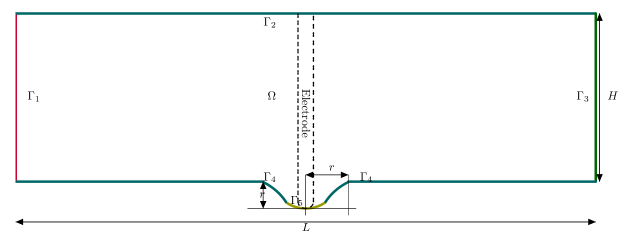
In the following, we fix values $L=1.5$, $H=0.5$ and $r=0.075$. We also assume that the thickness of the electrode is negligible, and we abound its effect in the numerical simulations. We prescribe the model boundaries, $\Gamma_{D}$ and $\Gamma_{N}$ of the mathematical model in terms of $\Gamma_{i},i=1,\cdots,5$ for each numerical test. For the time discretization, fixing an integer $M$, we define a time subdivision $t_{0}=0<\cdots<t_{M}=T$ and the time steps as $\tau_{n}={t_{n+1}-t_{n}},i=0,\cdots,M-1$. While we use a finite element discretization in space. Namely, we exploit the finite element P1-Bubble to compute the values of the velocity variable and the P1 finite element to approximate the temperature, pressure and potential unknowns. In the sequel, we keep the same notations of the variables $\boldsymbol{v}$, $P$, $\theta$ and $\varphi$ for the discrete versions.

Based on the specifications given in the literature, e.g., [26, 25, 27], we set the electrical, thermal, and flow-related material properties of the model components as follows. The electrical conductivity $\sigma$, thermal conductivity $\eta$, and blood conductivity $\nu$ have been modeled as a temperature-dependent function and are given by the following equation

$$\sigma(\theta) = \left\{\begin{array}[]{ll}\sigma_{0}\exp^{0.015\left(\theta-\theta_{b}\right)}&\text{ for }\theta\leq 99^{\circ}\mathrm{C}\\ 2.5345\sigma_{0}&\text{ for }99^{\circ}\mathrm{C}<\theta\leq 100^{\circ}\mathrm{C}\\ 2.5345\sigma_{0}\left(1-0.198\left(\theta-100^{\circ}\mathrm{C}\right)\right)&\text{ for }100^{\circ}\mathrm{C}<\theta\leq 105^{\circ}\mathrm{C}\\ 0.025345\sigma_{0}&\text{ for }\theta>105^{\circ}\mathrm{C}\end{array}\right.$$

$$\eta(\theta) = \left\{\begin{array}[]{ll}\eta_{0}+0.0012\left(\theta-\theta_{b}\right)&\text{ for }\theta\leq 100^{\circ}\mathrm{C}\\ \eta_{0}+0.0012\left(100^{\circ}\mathrm{C}-\theta_{b}\right)&\text{ for }\theta>100^{\circ}\mathrm{C}\end{array}\right.$$

where $\sigma_{0}=0.6$ and $\eta_{0}=0.54$ are the constant electrical conductivity and the thermal conductivity, respectively, at core body temperature, $\theta_{b}\left(=37^{\circ}\mathrm{C}\right)$. The viscosity and density of blood are $0.0021\mathrm{~{}Pa}\cdot\mathrm{s}$ and $1000\mathrm{~{}kg}/\mathrm{m}^{3}$, respectively, whereas those of saline are $0.001\mathrm{~{}Pa}\cdot\mathrm{s}$ and $1000\mathrm{~{}kg}/\mathrm{m}^{3}$, respectively, based on the material property of water.

We now deal with the reformulation of the studied model into an algebraic system of differential equations that allows us to use a time lag scheme. That is, given the solution of the heat equation at the previous time, we solve then the decoupled potential and Navier-Stokes equations (21)-(20) for time step $n-1$ as

$$\left\{\begin{array}[]{rclll}\boldsymbol{v}_{t}-\nabla\cdot(\nu({\theta}^{n-1})\mathbb{D}(\boldsymbol{v}))+\nabla\cdot(\boldsymbol{v}\otimes\boldsymbol{v})+\nabla P&=&\boldsymbol{F}({\theta}^{n-1})&\hbox{ in }\Omega_{T}\\ \nabla\cdot\boldsymbol{v}&=&0&\hbox{ in }\Omega_{T}\\ \boldsymbol{v}&=&0&\hbox{ on }\Sigma_{D}\\ -P\boldsymbol{n}+\nu({\theta}^{n-1})\mathbb{D}(\boldsymbol{v})\boldsymbol{n}&=&\mathbf{0}&\hbox{ on }\Sigma_{N}\\ \boldsymbol{v}(\boldsymbol{x},0)&=&\boldsymbol{v}_{0}(\boldsymbol{x})&\hbox{ in }\hbox{ }\Omega\end{array}\right.\hbox{ , }\left\{\begin{array}[]{rclll}-\operatorname{div}(\sigma({\theta}^{n-1})\nabla\varphi)&=&0&\hbox{ in }&\Omega_{T}\\ (\sigma({\theta}^{n-1})\nabla\varphi)\cdot\boldsymbol{n}&=&g&\hbox{ on }&\Sigma_{N}\\ \varphi&=&0&\hbox{ on }&\Sigma_{D}\\ \end{array}\right.$$ (101)

We get then the potential $\varphi^{n-1}$, the velocity $\boldsymbol{v}^{n-1}$ and the the pressure $P^{n-1}$ at the time step $n-1$. We solve then the temperature equation at time $n$.
A more interesting question is how to treat the temperature advection-diffusion equation. By default, not all discretizations of this equation are equally stable unless we use regularization techniques. To achieve this, we can use discontinuous elements which is more efficient for pure advection problems. But in the presence of diffusion terms, the discretization of the Laplace operator is cumbersome due to the large number of additional terms that must be integrated on each face between the cells. A better alternative is therefore to add some nonlinear viscosity $\tilde{\eta}(\theta)$ to the model that only acts in the vicinity of shocks and other discontinuities. $\tilde{\eta}(\theta)$ is chosen in such a way that if $\theta$ satisfies the original equations, the additional viscosity is zero. To achieve this, the literature contains a number of approaches. We will opt here for the stabilization strategy developed by Guermond and Popov [28] that builds on a suitably defined residual and a limiting procedure for the additional viscosity. To this end, let us define a residual $R_{\alpha}(\theta)$ as follows:

$$R_{\alpha}(\theta)=\left(\frac{\partial\theta}{\partial t}+\boldsymbol{v}\cdot\nabla\theta-\nabla\cdot\eta(\overline{\theta})\nabla\theta-\displaystyle\nu(\overline{\theta})\mathbb{D}(\boldsymbol{v}):\mathbb{D}(\boldsymbol{v})-\sigma(\overline{\theta})|\nabla\varphi|^{2}\right)\theta^{\alpha-1},\quad\alpha\in[1,2].$$

Note that $R_{\alpha}(\theta)$ will be zero if $\theta$ satisfies the temperature equation. Multiplying terms out, we get the following, entirely equivalent form:

$$R_{\alpha}(\theta)=\frac{1}{\alpha}\frac{\partial\left(\theta^{\alpha}\right)}{\partial t}+\frac{1}{\alpha}\boldsymbol{v}\cdot\nabla\left(\theta^{\alpha}\right)-\frac{1}{\alpha}\nabla\cdot\eta(\overline{\theta})\nabla\left(\theta^{\alpha}\right)+\eta(\overline{\theta})(\alpha-1)\theta^{\alpha-2}|\nabla\theta|^{2}-\gamma\theta^{\alpha-1}.$$

Using the latter, we can define the artificial viscosity as a piecewise constant function defined on each cell $K$ with diameter $h_{K}$ separately as follows:

$$\left.\tilde{\eta}_{\alpha}(\theta)\right|_{K}=\beta\|\boldsymbol{v}\|_{L^{\infty}(K)}\min\left\{h_{K},h_{K}^{\alpha}\frac{\left\|R_{\alpha}(\theta)\right\|_{L^{\infty}(K)}}{c(\boldsymbol{v},\theta)}\right\}$$

where, $\beta$ is a stabilization constant and $\displaystyle c(\boldsymbol{v},\theta)=c_{R}\|\boldsymbol{v}\|_{L^{\infty}(\Omega)}\operatorname{var}(\theta)|\operatorname{diam}(\Omega)|^{\alpha-2}$ where $\operatorname{var}(\theta)=\max_{\Omega}\theta-\min_{\Omega}\theta$ is the range of present temperature values and $c_{R}$ is a dimensionless constant.
If on a particular cell the temperature field is smooth, then we expect the residual to be small and the stabilization term that injects the artificial diffusion will be rather small, when no additional diffusion is needed. On the other hand, if we are on or near a discontinuity in the temperature field, then the residual will be large and the artificial viscosity will ensure the stability of the scheme.

We start our simulation with the following configurations. We impose a velocity ${\boldsymbol{v}}=\left(\begin{array}[]{l}y(H-y)\\ 0\end{array}\right)$ on boundary $\Gamma_{1}$, ${\boldsymbol{v}}=\left(\begin{array}[]{l}\displaystyle\frac{2}{r}(x-\frac{L}{2}+r)(\frac{L}{2}+r-x)(\frac{L}{2}-x)\\ \displaystyle\frac{-2}{r}(x-\frac{L}{2}+r)(\frac{L}{2}+r-x)y\end{array}\right)$ on boundary $\Gamma_{5}$, and on boundaries $\Gamma_{i},i=2,4$, we assume that the velocity is zero. While on the 3th boundary $\Gamma_{3}$, we assume that $-\mathbb{S}(\boldsymbol{v},P)\boldsymbol{n}=\mathbf{0}$. Concerning the temperature, on the boundaries $\Gamma_{i}$, $i=1,2,4$, we apply the condition $(\eta(\theta)\nabla\theta)\cdot\boldsymbol{n}+\alpha\theta=\alpha\theta_{l}$, with $\alpha=1$ and $\theta_{l}=\theta_{b}=37$. On $\Gamma_{3}$, we impose an artificial boundary condition, that is the homogeneous Neumann boundary conditions. While on $\Gamma_{5}$, we assume that the saline heat is $20$. For the potential equation, we fix $g=5$ on $\Gamma_{5}$ and the homogeneous Dirichlet condition in the remaining boundaries. In this test, we neglect the second member of the Navier-Stokes equations, so $\mathbf{F}=0$. The initial conditions for the heat transport equation and the Navier-Stokes system are constructed by solving the associated stationary equation.
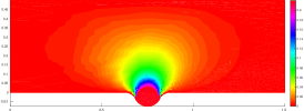
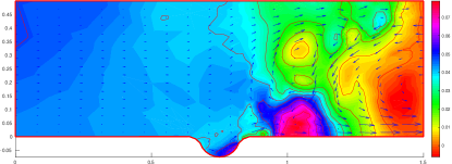
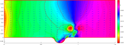
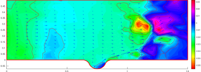
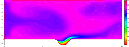
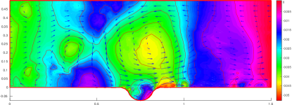
We then focus our reading for this test on the influence of the presence of the energy dissipation term due to viscosities $\displaystyle\nu(\theta)\mathbb{D}(\boldsymbol{v}):\mathbb{D}(\boldsymbol{v})$ and $\displaystyle\lambda(\theta)\nabla\varphi\cdot\nabla\varphi$. As we see in the potential figures (Figure 3 - column 3), with data $g>0$ on $\Gamma_{5}$ (the head of the electrode), we create a potential with a higher density in a neighborhood of the border $\Gamma_{5}$. 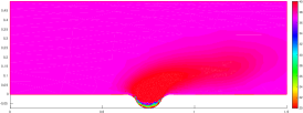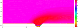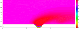In the same neighborhood, a temperature is produced. This shows the impact of the quadratic term $\displaystyle\lambda(\theta)\nabla\varphi\cdot\nabla\varphi$ as an energy source for the heat equation (Figure 3 - column 1). However, when there is a blood flow, the temperature produced will be moved to the outlet of the domain. This is a consequence of the transport term $\boldsymbol{v}\cdot\nabla T$. 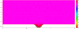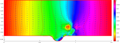In order to present these evolutions, we show in Figure 3 the results of numerical simulations at five different times $t=0$, $t=\frac{T}{4}$, $t=\frac{T}{2}$, $t=\frac{3T}{4}$ and $t=T$, where each row of the figure represents the corresponding time in the same order. 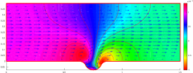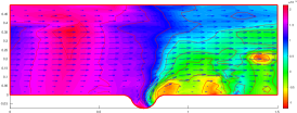In the first column, we show the heat transport. In the second column, we show the velocity field and the pressure, and in the third column, we show the potential intensity.

Figure 3: Test 1 : evolution of heat (column 1), velocity and pressure (column 2), and potential (column 3) at five time moments $t=0$ (line 1), $t=\frac{T}{4}$ (line 2), $t=\frac{T}{2}$ (line 3), $t=\frac{3T}{4}$ (line 4) and $t=T$ (line 5).

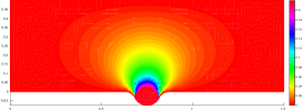
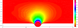
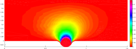
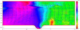
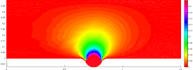
We notice that the potential evolves very slowly during the time iterations. This can be justified by the fact that the only data in the potential equation is the source $g$ which is constant and the electrical conductivity $\sigma(\theta)=\sigma_{0}\exp(0.015(\theta-\theta_{b}))$. As the temperature changes are counted between $38$ and $40$ as a maximum value, evolving the electrical conductivity at these points we find that $\sigma$ varies between $0.627$ and $0.610$, i.e. a variation of the order $10^{-2}$. This is consistent with the results obtained. This remark is also applicable to the velocity field. Indeed, we notice that the motion of the fluid is almost the same during the time iterations, except in small regions of the intersection of the saline fluid and the blood.

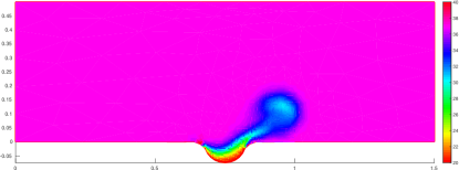
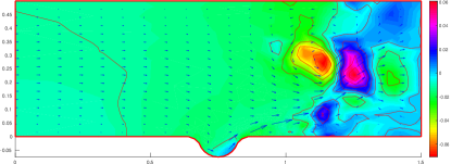
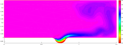
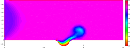
In the sequel, we are interested in the behavior of the heat when the fluid source term is non-zero, and also if we change the boundary condition in $\Gamma_{3}$. Impose a boundary condition on $\Gamma_{3}$ so as to limit the heat exchange with the exterior. Let us then consider the condition $(\eta(\theta)\nabla\theta)\cdot\boldsymbol{n}+\alpha\theta=\alpha\theta_{l}$ also on $\Gamma_{3}$, take the fluid source $\boldsymbol{F}=-\left(\begin{array}[]{l}0\\ 10^{-3}9.81/303\left(\theta-\theta_{b}\right)\end{array}\right)$ as in Boussinesq equations, and decrease $g$ to $1$.
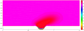
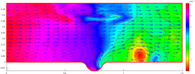
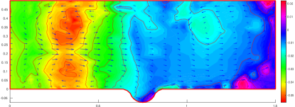
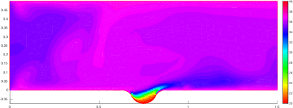
We omit here the figures of the solutions at the initial iterations since they are almost the same as in the previous test. We also omit the figures of the potential as there is no significant change during the iterations. We represent on Figure 4 the evolution of the heat (first column) and of the velocity and pressure (column 2) at times $t=\frac{T}{8}$, $t=\frac{T}{4}$, $t=\frac{T}{2}$ and $t=T$. We notice that decreasing $g$ involves a diminution of the potential in the domain and consequently the calculated heat is reduced. This allowed the possibility of cooling the domain by the saline fluid from $\Gamma_{5}$ (see Figure 4 - colomn 1). We also observe the rotation of the fluid in the areas subject to heat variations, especially in the area near the outlet boundary $\Gamma_{3}$. A result that we justify by the structure of the source term $F$, in particular the term $\theta-\theta_{b}$, indeed by the principle of maximum the velocity changes its sign according to the value of the temperature $\theta$ whether it is lower or higher than $\theta_{b}$. With this configuration we achieve a reduction of the temperature in certain areas of the domain. But this ceases to work from a certain level and the heat will be equilibrated because of the domain’s homogeneity. For this we can add other cooling factors. 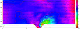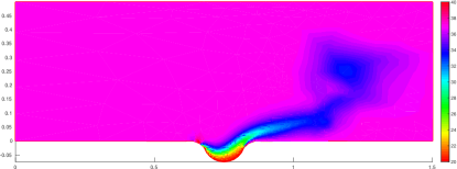We assume in the following test that the heat of the fluid will enter through $\Gamma_{1}$ with a different temperature than the domain one, i.e. $\theta=35$. The results of this choice are shown in Figure 5 with the same descriptions as in Figure 4.

Figure 4: Test 2 : evolution of heat (column 1), velocity and pressure (column 2) at four time moments $t=\frac{T}{8}$ (line 1), $t=\frac{T}{4}$ (line 2), $t=\frac{T}{2}$ (line 3) and $t=T$ (line 4).

Figure 5: Test 3 : evolution of heat (column 1), velocity and pressure (column 2) at four time moments $t=\frac{T}{8}$ (line 1), $t=\frac{T}{4}$ (line 2), $t=\frac{T}{2}$ (line 3) and $t=T$ (line 4).

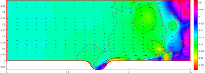
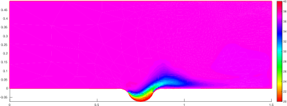
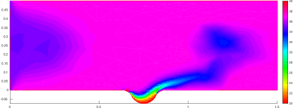
Let us now return to the effects of the source and dissipation terms. In fact, for quite large values of $g$, we have marked a rapid increase in the temperature as well as in the order of rotation of the fluid. Thus, we arrive at an explosion of the values.

5 Conclusion and perspectives

In this paper, a nonlinear fluid-heat-potential system modeling radiofrequency ablation phenomena in cardiac tissue has been proposed. The existence of the global solutions using Schauder’s fixed-point theory has been demonstrated, as well as their uniqueness under some additional conditions on the data, both in two-dimensional and three-dimensional space. Numerical simulations in different cases have been illustrated in a two-dimensional space using the finite element method.

The phenomena of radiofrequency ablation in different tissues are procedures that make it possible to predict the temperature of the tissues during these procedures. For this reason, we believe that this work opens up interesting perspectives, such as optimal control models and inverse problems, namely the identification of the frequency factor of different types of tissue.

As we were equipped in the last section, for $g$ large enough, we notice a rapid increase in temperature as well as in the order of rotation of the fluid. This motivates us to study particular cases where the source terms are less regular, the case $L^{1}$ for example.

Other perspectives consist in deriving system (1) from a kinetic-fluid model. This can improve our knowledge from the modeling point of view, as the kinetic (mesoscopic) scale gives a more detailed insight into the interactions of the cells. However, for more details, we refer the interested reader to [8]. Another interesting perspective could be to consider the stochastic aspect, see [10, 11, 42].

References

- Adams [1975] Adams, R et Fournier, J., 1975. espaces de sobolev, acad. Presse, New York 19.
- Adams [2003] Adams, Robert A et Fournier, J., 2003. Espaces de sobolev mathématiques pures et appliquées (amsterdam), 140.
- Ahmed et al. [2008] Ahmed, M., Liu, Z., Humphries, S., Nahum Goldberg, S., 2008. Computer modeling of the combined effects of perfusion, electrical conductivity, and thermal conductivity on tissue heating patterns in radiofrequency tumor ablation. International Journal of Hyperthermia 24, 577–588.
- Akrivis and Larsson [2005] Akrivis, G., Larsson, S., 2005. Linearly implicit finite element methods for the time-dependent joule heating problem. BIT Numerical Mathematics 45, 429–442.
- Allegretto et al. [1999] Allegretto, W., Liu, Y., Zhou, A., 1999. A box scheme for coupled systems resulting from microsensor thermistor problems. Dynamics of continuous discrete and impulsive systems 5, 209–223.
- Allegretto and Xie [1992] Allegretto, W., Xie, H., 1992. Existence of solutions for the time-dependent thermistor equations. IMA Journal of Applied Mathematics 48, 271–281.
- Antonietti et al. [2022] Antonietti, P.F., Vacca, G., Verani, M., 2022. Virtual element method for the navier–stokes equation coupled with the heat equation. arXiv preprint arXiv:2205.00954 .
- Atlas et al. [2020] Atlas, A., Bendahmane, M., Karami, F., Meskine, D., Zagour, M., 2020. Kinetic-fluid derivation and mathematical analysis of a nonlocal cross-diffusion-fluid system. Appl. Math. Model. 82, 379–408.
- Aubin [1963] Aubin, J.P., 1963. Un thorme de compacit. CR Acad. Sci. Paris 256, 3.
- Bendahmane et al. [2023] Bendahmane, M., Nzeti, H., Tagoudjeu, J., Zagour, M., 2023. Stochastic reaction–diffusion system modeling predator–prey interactions with prey-taxis and noises. Chaos 33, Paper No. 073103, 26.
- Bendahmane et al. [2022] Bendahmane, M., Tagoudjeu, J., Zagour, M., 2022. Odd-Even based asymptotic preserving scheme for a 2D stochastic kinetic-fluid model. J. Comput. Phys. 471, Paper No. 111649, 25.
- Beneš [2011] Beneš, M., 2011. Strong solutions to non-stationary channel flows of heat-conducting viscous incompressible fluids with dissipative heating. Acta applicandae mathematicae 116, 237–254.
- Beneš and Kučera [2007] Beneš, M., Kučera, P., 2007. Non-steady navier-stokes equations with homogeneous mixed boundary conditions and arbitrarily large initial condition. Carpathian Journal of Mathematics , 32–40.
- Beneš et al. [2022] Beneš, M., Pažanin, I., Radulović, M., 2022. On viscous incompressible flows of nonsymmetric fluids with mixed boundary conditions. Nonlinear Analysis: Real World Applications 64, 103424.
- Beneš and Tichỳ [2015] Beneš, M., Tichỳ, J., 2015. On coupled navier–stokes and energy equations in exterior-like domains. Computers and Mathematics with Applications 70, 2867–2882.
- Berjano [2006] Berjano, E.J., 2006. Theoretical modeling for radiofrequency ablation: state-of-the-art and challenges for the future. Biomedical engineering online 5, 1–17.
- Bulíček et al. [2016] Bulíček, M., Diening, L., Schwarzacher, S., 2016. Existence, uniqueness and optimal regularity results for very weak solutions to nonlinear elliptic systems. Analysis & PDE 9, 1115–1151.
- Cimatti [1992] Cimatti, G., 1992. Existence of weak solutions for the nonstationary problem of the joule heating of a conductor. Annali di Matematica pura ed applicata 162, 33–42.
- Deteix et al. [2014] Deteix, J., Jendoubi, A., Yakoubi, D., 2014. A coupled prediction scheme for solving the navier–stokes and convection-diffusion equations. SIAM Journal on Numerical Analysis 52, 2415–2439.
- Deugoue et al. [2021] Deugoue, G., Djoko, J., Fouape, A., 2021. Globally modified navier-stokes equations coupled with the heat equation: existence result and time discrete approximation. Journal of Applied Analysis & Computation 11, 2423–2458.
- Elliott and Larsson [1995] Elliott, C.M., Larsson, S., 1995. A finite element model for the time-dependent joule heating problem. Mathematics of computation 64, 1433–1453.
- Formaggia et al. [2009] Formaggia, L., Quarteroni, A., Veneziani, A., 2009. Cardiovascular mathematics, volume 1 of ms&a. modeling, simulation and applications.
- Gao [2016] Gao, H., 2016. Unconditional optimal error estimates of bdf–galerkin fems for nonlinear thermistor equations. Journal of Scientific Computing 66, 504–527.
- Gatica [1988] Gatica, J.A., 1988. Ordinary differential equations: Introduction to the theory of ordinary differential equations in the real domain (jaroslav kurzweil). SIAM Review 30, 512.
- González-Suárez and Berjano [2015] González-Suárez, A., Berjano, E., 2015. Comparative analysis of different methods of modeling the thermal effect of circulating blood flow during rf cardiac ablation. IEEE Transactions on Biomedical Engineering 63, 250–259.
- González-Suárez et al. [2016] González-Suárez, A., Berjano, E., Guerra, J.M., Gerardo-Giorda, L., 2016. Computational modeling of open-irrigated electrodes for radiofrequency cardiac ablation including blood motion-saline flow interaction. PloS one 11, e0150356.
- González-Suárez et al. [2018] González-Suárez, A., Pérez, J.J., Berjano, E., 2018. Should fluid dynamics be included in computer models of rf cardiac ablation by irrigated-tip electrodes? Biomedical engineering online 17, 1–14.
- Guermond et al. [2011] Guermond, J.L., Pasquetti, R., Popov, B., 2011. Entropy viscosity method for nonlinear conservation laws. Journal of Computational Physics 230, 4248–4267.
- Johnson and Saidel [2002] Johnson, P.C., Saidel, G.M., 2002. Thermal model for fast simulation during magnetic resonance imaging guidance of radio frequency tumor ablation. Annals of Biomedical Engineering 30, 1152–1161.
- Kufner et al. [1977] Kufner, A., John, O., Fucik, S., 1977. Function spaces. volume 3. Springer Science & Business Media.
- Li et al. [2014] Li, B., Gao, H., Sun, W., 2014. Unconditionally optimal error estimates of a crank–nicolson galerkin method for the nonlinear thermistor equations. SIAM Journal on Numerical Analysis 52, 933–954.
- Li and Sun [2013] Li, B., Sun, W., 2013. Error analysis of linearized semi-implicit galerkin finite element methods for nonlinear parabolic equations. International Journal of Numerical Analysis and Modeling 10, 622–633.
- Li and Yang [2015] Li, B., Yang, C., 2015. Uniform bmo estimate of parabolic equations and global well-posedness of the thermistor problem, in: Forum of Mathematics, Sigma, Cambridge University Press.
- Mbehou [2018] Mbehou, M., 2018. The theta-galerkin finite element method for coupled systems resulting from microsensor thermistor problems. Mathematical Methods in the Applied Sciences 41, 1480–1491.
- Meinlschmidt et al. [2017a] Meinlschmidt, H., Meyer, C., Rehberg, J., 2017a. Optimal control of the thermistor problem in three spatial dimensions, part 1: Existence of optimal solutions. SIAM Journal on Control and Optimization 55, 2876–2904.
- Meinlschmidt et al. [2017b] Meinlschmidt, H., Meyer, C., Rehberg, J., 2017b. Optimal control of the thermistor problem in three spatial dimensions, part 2: Optimality conditions. SIAM Journal on Control and Optimization 55, 2368–2392.
- Miroslav et al. [2009] Miroslav, B., Eduard, F., Josef, M., 2009. A navier–stokes–fourier system for incompressible fluids with temperature dependent material coefficients. Nonlinear Analysis: Real World Applications 10, 992–1015.
- Nolte et al. [2021] Nolte, T., Vaidya, N., Baragona, M., Elevelt, A., Lavezzo, V., Maessen, R., Schulz, V., Veroy, K., 2021. Study of flow effects on temperature-controlled radiofrequency ablation using phantom experiments and forward simulations. Medical Physics 48, 4754–4768.
- Quarteroni et al. [2017] Quarteroni, A., Manzoni, A., Vergara, C., 2017. The cardiovascular system: mathematical modelling, numerical algorithms and clinical applications. Acta Numerica 26, 365–590.
- Villard et al. [2005] Villard, C., Soler, L., Gangi, A., 2005. Radiofrequency ablation of hepatic tumors: simulation, planning, and contribution of virtual reality and haptics. Computer Methods in Biomechanics and Biomedical Engineering 8, 215–227.
- Yuan and Liu [1994] Yuan, G., Liu, Z., 1994. Existence and uniqueness of the cα solution for the thermistor problem with mixed boundary value. SIAM Journal on Mathematical Analysis 25, 1157–1166.
- Zagour [2023] Zagour, M., 2023. Toward multiscale derivation of behavioral dynamics: Comment to “what is life? active particles tools towards behavioral dynamics in social-biology and economics”, by b. bellomo, m. esfahanian, v. secchini, and p. terna. Physics of Life Reviews 46, 273–274.