Simplicial Representation Learning with Neural $k$-Forms

Abstract

Geometric deep learning extends deep learning to incorporate information about the geometry and topology data, especially in complex domains like graphs. Despite the popularity of message passing in this field, it has limitations such as the need for graph rewiring, ambiguity in interpreting data, and over-smoothing. In this paper, we take a different approach, focusing on leveraging geometric information from simplicial complexes embedded in $\mathbb{R}^{n}$ using node coordinates. We use differential $k$-forms in $\mathbb{R}^{n}$ to create representations of simplices, offering interpretability and geometric consistency without message passing. This approach also enables us to apply differential geometry tools and achieve universal approximation. Our method is efficient, versatile, and applicable to various input complexes, including graphs, simplicial complexes, and cell complexes. It outperforms existing message passing neural networks in harnessing information from geometrical graphs with node features serving as coordinates.

1 Introduction

Geometric deep learning (Bronstein et al., 2017) expanded the scope of deep learning methods to include information about the geometry–and, to a lesser extent, topology—of data, thus enabling their use in more complicated and richer domains like graphs. While the recent years have seen the development of a plethora of methods, the predominant paradigm of the field remains message passing (Veličković, 2023), which was recently extended to handle higher-order domains, including simplicial complexes (Ebli et al., 2020), cell complexes (Hajij et al., 2020), and hypergraphs (Heydari & Livi, 2022). However, despite its utility, the message passing paradigm is seen to increasingly suffer from inherent limitations, requiring graph rewiring (Gasteiger et al., 2019) or other strategies to prevent over-smoothing (Topping et al., 2022).

Our paper pursues a completely different path and strives to leverage additional geometric information from a data set to obtain robust and interpretable representations of the input data. Specifically, we consider input data in the form of simplicial complexes embedded in $\mathbb{R}^{n}$ via node coordinates. This type of complex can be built from any graph with node features, with node features acting as the coordinates, for example. Our key insight is the use of differential $k$-forms in $\mathbb{R}^{n}$. A $k$-form in $\mathbb{R}^{n}$ can integrated over any $k$-simplex embedded in $\mathbb{R}^{n}$ to produce a real number. Thus an $\ell$-tuple of $k$-forms produces an $\ell$-dimensional representation of the simplex independently of any message passing. From this perspective, $k$-forms play the role of globally consistent feature maps over the space of embedded $k$-simplices, possessing the geometric semantics and interpretability of integration. This enables us to use tools from differential geometry to prove a version of universal approximation, as well as a number of other theoretical results. Moreover, the structure of differential forms in $\mathbb{R}^{n}$ makes learning algorithms (computationally) feasible. In particular, a multi-layer perceptron with the right dimensions induces a $k$-form on $\mathbb{R}^{n}$ that can be integrated. This implies that learnable, finitely-parametrised differential forms can be woven into existing machine learning libraries and applied to common tasks in geometric deep learning. We find that our method is better capable of harnessing information from geometrical graphs than existing message passing neural networks. Next to being efficient, our method is also generally applicable to a wide variety of input complexes, including graphs, simplicial complexes, and cell complexes.

Organisation of Paper

We present the relevant background for simplicial complexes and differential forms in Section 2. In Section 3 we present the concept of neural $k$-forms and prove a universal approximation statement. We then show how neural $k$-forms induce a so-called integration matrix in Section 4, and use the properties of integration to prove a number of propositions. Finally, in Section 5, we perform a number of intuitive experiments and benchmark our method on standard examples in the graph and geometric deep learning literature.

Related Work

Several papers already focus on generalising graph neural networks (GNNs) to higher-dimensional domains, proposing simplicial neural networks (Ebli et al., 2020; Bodnar et al., 2021b; Bunch et al., 2020; Roddenberry et al., 2021; Keros et al., 2022; Giusti et al., 2022; Goh et al., 2022), methods that are capable of leveraging higher-order topological features of data (Hajij et al., 2023; Hensel et al., 2021; Horn et al., 2022), or optimisation algorithms for learning representations of simplicial complexes (Hacker, 2020). All of these methods operate on simplicial complexes via diffusion processes or message passing algorithms. Some works also extend message passing or aggregation schemes to cell complexes (Bodnar et al., 2021a; Hajij et al., 2020; 2023) or cellular sheaves (Hansen & Gebhart, 2019; Barbero et al., 2022). However, there are some limitations to the aforementioned methods, arising from the use of message passing or aggregation along a combinatorial structure. This process often results in over-smoothing (a regression to the mean for all node features, making them indistinguishable) or over-squashing (an inability to transport long-range node information throughout the graph), necessitating additional interventions such as graph rewiring (Gasteiger et al., 2019; Nguyen et al., 2023; Topping et al., 2022). Hence, there is a need for methods that go beyond message passing. Our work provides a novel perspective based on the integration of learnable $k$-forms on combinatorial domains like graphs or simplicial complexes embedded in $\mathbb{R}^{n}$, i.e. we assume the existence of (node/vertex) coordinates.

2 Background

This section introduces the required background of simplicial complexes and differential forms. We restrict our focus to simplices and differential forms in $\mathbb{R}^{n}$, given this is the only setting we will use in practice to make the theory more accessible. For additional background references, we recommend Nanda (2021) for computational topology and Lee (2003); Tao (2009) for differential forms.

Simplicial Complexes and Geometric Realisations

A combinatorial simplicial complex on a non-empty set $\mathcal{S}^{0}$ is a collection $\mathcal{S}$ of non-empty subsets of $\mathcal{S}^{0}$ satisfying, (1) that $\{v\}\in\mathcal{S}$ for each $v\in\mathcal{S}^{0}$, and (2) that if $\sigma\in\mathcal{S}$ and $\tau\subset\sigma$ then $\tau\in\mathcal{S}$. The complex is oriented if there is an ordering on the elements of $V$. The subsets of cardinality $(k+1)$ are called the $k$-dimensional simplices (or $k$-simplices) of $\mathcal{S}$, this set is denoted by $\mathcal{S}^{k}$. We denote the convex hull of $k$ points $x_{0},x_{1},\ldots,x_{k}$ in $\mathbb{R}^{n}$ by $[x_{0},x_{1},\ldots,x_{k}]$. Given a map $\phi\colon\mathcal{S}^{0}\to\mathbb{R}^{n}$, the (linear) geometric realisation of $\mathcal{S}$ with respect to $\phi$ is the subspace of $\mathbb{R}^{n}$ given by $\lvert\mathcal{S}\rvert_{\phi}=\bigcup_{\sigma\in\mathcal{S}}\lvert\sigma\rvert_{\phi}$, where $\lvert\sigma\rvert_{\phi}$ is the convex hull $[\phi(v_{0}),\phi(v_{1}),\ldots,\phi(v_{k})]$ of the embedded vertices of $\mathcal{S}^{0}$. The standard geometric $k$-simplex is the subspace of $\mathbb{R}^{k}$ given by $\Delta^{k}=[t_{0},t_{1},\ldots,t_{k}]$ where $t_{0}=0$ and $t_{i}$ is the standard orthonormal $i$-th basis vector in $\mathbb{R}^{k}$. The embedding of $\mathcal{S}$ determines a unique linear map ${\left.\kern-1.2pt\phi\vphantom{\big{|}}\right|_{\sigma}}\colon\Delta^{k}\to\mathbb{R}^{n}$ for every $\sigma\in\mathcal{S}^{k}$ and $k\in\mathbb{N}$ which is determined by mapping the vertices $t_{0},t_{1},\ldots,t_{k}$ of $\Delta^{k}$ to the embedded vertices $\phi(v^{\sigma}_{1}),\phi(v^{\sigma}_{2})\ldots\phi(v^{\sigma}_{k})$ of $\sigma$. We will often denote the embedding function over the entire complex by $\phi:\mathcal{S}\to\mathbb{R}^{n}$.

Chains and Cochains over $\mathbb{R}$

For an oriented simplicial complex $\mathcal{S}$, the simplicial $k$-chains $C_{k}(\mathcal{S};\mathbb{R})$ is the vector space

$$C_{k}(\mathcal{S};\mathbb{R})=\Bigg{\{}\sum_{i}\lambda_{i}\sigma_{i}\mid\sigma_{i}\in\mathcal{S}^{k},\lambda_{i}\in\mathbb{R}\Bigg{\}}$$ (1)

of formal linear combinations of $k$-simplices in $\mathcal{S}$. The simplicial $k$-cochains $C^{k}(\mathcal{S};\mathbb{R})$ over $\mathbb{R}$ is the dual space $\mathsf{Hom}(C_{k}(\mathcal{S});\mathbb{R})$ of linear functionals over the simplicial $k$-chains. A (smooth) singular simplex in $\mathbb{R}^{n}$ is a continuous (resp. smooth) map $\sigma\colon\Delta^{k}\to\mathbb{R}^{n}$. Similar to above, the singular $k$-chains is the (infinite dimensional) $\mathbb{R}$-vector space

$$C_{k}^{sing}(\mathbb{R}^{n};\mathbb{R})=\Bigg{\{}\sum_{i}\lambda_{i}\sigma_{i}\mid\sigma_{i}:\Delta^{k}\to\mathbb{R}^{n},\lambda_{i}\in\mathbb{R}\Bigg{\}}$$ (2)

consisting of finite formal linear combinations of singular simplices in $\mathbb{R}^{n}$. The singular cochains $C^{k}_{sing}(\mathbb{R}^{n})$ over $\mathbb{R}$ is the dual space $\mathsf{Hom}(C_{k}^{sing}(\mathbb{R}^{n});\mathbb{R})$ of linear functionals over the singular chains. When $\mathcal{S}$ has an embedding $\phi\colon\mathcal{S}\to\mathbb{R}^{n}$, there is a linear map

$$\phi^{*}\colon C^{k}_{sing}(\mathbb{R}^{n};\mathbb{R})\to C^{k}(\mathcal{S};\mathbb{R}),$$ (3)

which takes a singular cochain $\gamma\in C^{k}_{sing}(\mathbb{R}^{n};\mathbb{R})$ to the simplicial cochain determined by the formula $\phi^{*}\gamma(\sigma)=\gamma({\left.\kern-1.2pt\phi\vphantom{\big{|}}\right|_{\sigma}})$.

Differential Forms

Intuitively, a differential form in $\mathbb{R}^{n}$ is a function that assigns volume to $k$-vectors $v_{1}\otimes v_{2}\otimes\ldots\otimes v_{k}$ of tangent vectors $v_{i}\in T_{p}(\mathbb{R}^{n})$ at a point $p\in\mathbb{R}^{n}$. The space of $k$-vectors at a point $p$ is formalised algebraically as the $k$-th tensor product $\otimes_{k}T_{p}(\mathbb{R}^{n})$ (see Appendix A). A $k$-form $\omega\in\Omega^{k}(\mathbb{R}^{n})$ locally acts like a multi-linear alternating function $\omega_{p}:\bigotimes_{k}T_{p}(\mathbb{R}^{n})\to\mathbb{R}$ at every point $p\in\mathbb{R}^{n}$: $\omega_{p}$ take as input a $k$-vector $v_{1}\otimes v_{2}\otimes\ldots\otimes v_{k}$ in the $k$-th tensor of the tangent space at $p$ and outputs a real number. Alternating multi-linearity is a generalisation of the properties of the determinant as a measure of signed volume. Thus, one interprets this number as the oriented volume of the $k$-tangent vector $v_{1}\otimes v_{2}\otimes\ldots\otimes v_{k}$ with respect to $\omega$. There is an isomorphism between $1$-forms and vector fields in $\mathbb{R}^{n}$ which enables visualizing $1$-forms in practice. Namely, a vector field $\eta:\mathbb{R}^{n}\to T_{*}(\mathbb{R}^{n})$ corresponds to a unique $1$-form $\omega$ which evaluates on $v\in T_{p}(\mathbb{R}^{n})$ by $\omega_{p}(v)=\langle\eta(p),v\rangle_{p}$ where the inner product is induced by the standard Riemannian structure on $\mathbb{R}^{n}$.

Standard Decomposition

Let $x_{1},x_{2},\ldots,x_{n}:\mathbb{R}^{n}\to\mathbb{R}$ be the standard coordinate functions. Each of these features an assigned $1$-form $dx_{i}\in\Omega^{1}(\mathbb{R}^{n})$ called the differential of $x_{i}$, which is locally the linear dual to the unit vector field $\partial/\partial x_{i}$ in direction $x_{i}$. A multi-index $I$ of length $k$ is an ordered $k$-tuple $(i_{1},\ldots,i_{k})$ of positive integers. For a multi-index $I$ of length $k$ and $p\in\mathbb{R}^{n}$, the $k$-form $dx_{I}:=dx_{i_{1}}\wedge\ldots\wedge d{x_{i_{k}}}$ is the differential form that returns the standard volume of a $k$-parallelepiped projected in the $k$-subspace of the tangent space $T_{p}{\mathbb{R}^{n}}$ spanned by the dimensions in $I$. Multi-indices allow us to express $k$-forms $\omega\in\Omega^{k}(\mathbb{R}^{n})$ in a useful canonical form, i.e.

$$\omega=\sum\alpha_{I}dx_{I},$$ (4)

where $I$ ranges over all $\binom{n}{k}$ strictly increasing multi-indices of length $k$. The scaling functions $\alpha_{I}\colon\mathbb{R}^{n}\to\mathbb{R}$ induce multi-linear alternating functions $\omega_{p}=\sum\alpha_{I}(p)(dx_{I})_{p}\colon\bigotimes_{k}T_{p}\mathbb{R}^{n}\to\mathbb{R}.$. Intuitively, $\alpha_{I}\colon\mathbb{R}^{n}\to\mathbb{R}$ describes an oriented rescaling of an infinitesimal $k$-volume in the $I$-subspace at each tangent space $T_{p}(\mathbb{R}^{n})$. We call a $k$-form compactly supported/smooth/linear if the scaling functions $\alpha_{I}$ are compactly supported/smooth/linear, respectively (see Appendix A).

Integration

Sufficiently well-behaved $k$-forms can be a integrated over $k$-simplices smoothly embedded in $\mathbb{R}^{n}$ to produce a real value. Let $D\phi(t)$ be the Jacobian matrix of $\phi$ at $t\in\Delta^{k}$. Let $\varepsilon^{I}:M^{n\times k}(\mathbb{R})\to\mathbb{R}$ be the function that evaluates the determinant of the $I$-rows of a matrix $M$ for a multi-index $I=(i_{1},\ldots,i_{k})$. In our setting, the integral of $\omega$ over $\phi$ can be expressed as

$$\int_{\phi}\omega=\sum_{I}\int_{\Delta^{k}}\alpha_{I}(\phi(t))\varepsilon^{I}\big{(}D\phi(t)\big{)}dt$$ (5)

where the integral is interpreted as a standard Riemann integral over the (compact) subset $\Delta^{k}\subseteq\mathbb{R}^{k}$. Equation 5 implies that the integral is well-defined if $\phi$ is a $C^{1}$ embedding function and $\alpha_{I}\circ\phi$ is integrable. In practice, this integral is approximated with a finite Riemann sum. We provide more background on integration of forms in Appendix A.

3 Neural $k$-Forms

Neural $k$-forms

Drawing on the decomposition of $k$-forms in Eq. 4, an MLP with the correct dimensions induces a $k$-form. For a multi-index $I$, let $\pi_{I}\colon\mathbb{R}^{\binom{n}{k}}\to\mathbb{R}$ be the projection onto the $I$-th component, noting that the length $k$ multi-indices over $n$ are in correspondence with the dimensions of $\mathbb{R}^{\binom{n}{k}}$. For brevity, we write $\psi_{I}:=\pi_{I}\circ\psi:\mathbb{R}^{\binom{n}{k}}\to\mathbb{R}$.

Definition 1.

Let $\psi\colon\mathbb{R}^{n}\to\mathbb{R}^{\binom{n}{k}}$ be an MLP. The neural $k$-form $\omega^{\psi}\in\Omega^{k}(\mathbb{R}^{n})$ associated to $\psi$ is the $k$-form $\omega^{\psi}=\sum_{I}\psi_{I}dx_{I}$.

Intuitively, the output dimensions in $\mathbb{R}^{\binom{n}{k}}$ of the MLP determine the scaling functions $\psi_{I}=\pi_{I}\circ\psi:\mathbb{R}^{n}\to\mathbb{R}^{\binom{n}{k}}\to\mathbb{R}$ of the neural $k$-form $\omega^{\psi}$. Using the standard decomposition in Equation 4, these functions completely specify $\omega^{\psi}$. In that case the activation function is a sigmoid function or $\tanh$, Definition 1 produces smooth $k$-forms, whereas for a ReLU activation function, one obtains piecewise linear $k$-forms. For an MLP of the form $\psi\colon\mathbb{R}^{n}\to\mathbb{R}^{\binom{n}{k}\times\ell}$, we think of $\psi$ as inducing a tuple of $\ell$ different ‘feature’ $k$-forms, all of which are learnable and depend on the parameters of the underlying MLP.

Cochains and Representation Learning

Representation learning is the process of turning data into vectors in $\mathbb{R}^{\ell}$, from which one can use the standard tools of machine learning to classify and predict attributes of the data. In graph learning, and simplicial learning more generally, data comes in the form of simplices and simplicial complexes. From the representation learning perspective, a tuple of $\ell$ singular cochains $\psi:=(\psi_{1},\ldots,\psi_{\ell})$ is equivalent to specifying an $\ell$-dimensional representation of every simplex $\sigma\colon\Delta^{k}\to\mathbb{R}^{n}$ by evaluating $\psi(\sigma)$ component-wise. Using this paradigm, we consider each singular cochain to be a feature map on the space of linear combinations of embedded simplices.

Learnable Cochains via Neural Forms

The space of all possible singular cochains is enormous and difficult to parse directly. Ideally, one wishes for a subset of singular cochains which depend on a finite number of learnable parameters. The integration of neural forms provides a natural, easy-to-implement and interpretable framework for constructing finitely-parametrisable, learnable singular cochains in practice. Indeed, integration of $k$-forms defines a linear map

$$\int\colon\Omega^{k}(\mathbb{R}^{n})\to C^{k}_{sing}(\mathbb{R}^{n};\mathbb{R})$$ (6)

called the De Rham map. For a $k$-form $\omega\in\Omega^{k}(\mathbb{R}^{n})$, the De Rham map returns the singular cochain $\int_{(-)}\omega\in C^{k}_{sing}(\mathbb{R}^{n})$ whose value on an embedded simplex $\phi\colon\Delta^{k}\to\mathbb{R}^{n}$ is given by $\int_{\phi}\omega\in\mathbb{R}$ using Equation 5 and is extended to chains linearly. Thus, a neural $k$-form $\omega^{\psi}$ induces a singular cochain $\int_{(-)}\omega^{\psi}$, which is finitely parametrised and learnable in practice.

Remark 2.

A neural $0$-form over $\mathbb{R}^{n}$ with $\ell$ features is an MLP $\psi$ from $\mathbb{R}^{n}$ to $\mathbb{R}^{\ell}$. The $0$-simplices $p\in\mathbb{R}^{n}$ are points in $\mathbb{R}^{n}$, and integration of a $0$-form corresponds to the evaluation $\psi(p)$. In this way, neural $k$-forms are a direct extension of MLPs to higher-dimensional simplices in $\mathbb{R}^{n}$.

Universal Approximation

We would like to know which $k$-forms on $\mathbb{R}^{n}$ are possible to approximate with neural $k$-forms. The following proposition translates the well-known Universal Approximation Theorem (Cybenko (1989); Hornik et al. (1989)) for neural networks into the language of neural $k$-forms. Here, the norm $\lVert\,\,\,\rVert_{\Omega_{c}(\mathbb{R}^{n})}$ on $k$-forms is induced by the standard Riemannian structure on $\mathbb{R}^{n}$, as explained in Appendix C.

Theorem 3.

Let $\alpha\in C(\mathbb{R},\mathbb{R})$ be a non-polynomial activation function. For every $n\in\mathbb{N}$ and compactly supported $k$-form $\eta\in\Omega^{k}_{c}(\mathbb{R}^{n})$ and $\epsilon>0$ there exists a neural $k$-form $\omega^{\psi}$ with one hidden layer such that $\lVert\omega^{\psi}-\eta\rVert_{\Omega_{c}(\mathbb{R}^{n})}<\epsilon$.

4 Integration Matrices

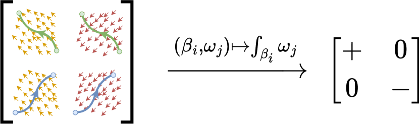
Figure 1: An integration matrix with data in dimension $1$, where embedded oriented $1$-simplices correspond to paths and $1$-forms are canonically identified with vector fields (see Appendix A for details). Integration of a $1$-form against a path corresponds to path integration against the respective vector field. Thus, integration of the paired paths and $1$-forms in the left matrix recovers real values with the signs given in the right matrix.

Most simplicial neural networks follow a similar procedure. The key step is that the $k$-simplices of each simplicial complex $\mathcal{S}$ are replaced with a matrix $X_{\mathcal{S}}(\beta,\gamma)$ containing a selection of $\ell$ simplicial cochains $(\gamma_{1},\ldots,\gamma_{\ell})$ as columns. This can be thought of as a matrix containing evaluations $\gamma_{j}(\beta_{i})$ with respect to some basis $(\beta_{1},\ldots,\beta_{s})$ for the simplicial $k$-chains $C_{k}(\mathcal{S};\mathbb{R})$. One issue with this approach is that there is no canonical initialisation when one starts with only the data of a set of embedded finite simplicial complexes. We address this issue by introducing the integration matrix induced by a neural $k$-form. This produces the same data type, but has the advantage that the feature cochains correspond to integration of the same form defined over the ambient space.

Integration Matrices

For an embedded finite simplicial complex, an $\ell$-tuple $\omega=(\omega_{1},\omega_{2},\ldots,\omega_{\ell})$ of $k$-forms induces a matrix suitable to simplicial learning algorithms in a natural way via integration. Let $\phi\colon\mathcal{S}\to\mathbb{R}^{n}$ be an embedding of a simplicial complex and $\beta=(\beta_{1},\beta_{2},\ldots,\beta_{m})\in C_{k}(\mathcal{S};\mathbb{R})$ be a set of specified $k$-chains.

Definition 4.

The integration matrix with respect to $\beta$ and $\omega$ is $X_{\phi}(\beta,\omega)=\big{[}\int_{\beta_{i}}\omega_{j}\big{]}_{i,j}.$

The integral of $\omega$ over a simplicial chain $\beta=\sum\lambda_{a}\sigma_{a}\in C_{k}(\mathcal{S};\mathbb{R})$ with respect to the embedding $\phi:\mathcal{S}\to\mathbb{R}^{n}$ corresponds to the integral

$$\int_{\beta}\omega=\sum\lambda_{a}\int_{\left.\kern-1.2pt\phi\vphantom{\big{|}}\right|_{\sigma_{a}}}\omega.$$ (7)

Using Definition 1, if $\psi\colon\mathbb{R}^{n}\to\mathbb{R}^{\binom{n}{k}\times\ell}$ is an MLP, then an integration matrix $X_{\phi}(\beta,\omega^{\psi})$ can be constructed using neural $k$-forms. From another perspective, the $\ell$-tuple of $k$-forms $(\omega_{1},\omega_{2},\ldots,\omega_{\ell})$ induces an $\ell$-tuple of simplicial cochains $C^{k}(\mathcal{S};\mathbb{R})$ on $\mathcal{S}$ via the composition

$$\Omega^{k}(\mathbb{R}^{n})\xrightarrow{\int}C^{k}_{sing}(\mathbb{R}^{n};\mathbb{R})\xrightarrow{\phi^{*}}C^{k}(\mathcal{S};\mathbb{R})$$ (8)

of the De Rham map from Eq. 6 and the restriction map from Eq. 3. Each column of the integration matrix $X_{\phi}(\beta,\omega)$ corresponds to evaluation of such a simplicial cochain over the $k$-chains $\beta=(\beta_{1},\beta_{2},\ldots,\beta_{m})$.

Remark 5 (Interpretability).

The key point is that the integration matrices of two different simplicial complexes $\phi\colon\mathcal{S}\to\mathbb{R}^{n}$ and $\phi^{\prime}\colon\mathcal{S}^{\prime}\to\mathbb{R}^{n}$ embedded in $\mathbb{R}^{n}$ have a shared interpretation. That is, the $j$-th column of both of their integration matrices corresponds to integration of their $k$-simplices against the same feature $k$-form $\omega_{j}\in\Omega^{k}(\mathbb{R}^{n})$.

Basic Properties

There are a number of useful basic properties about integration matrices that follow from the well-known properties of integration and theory of MLPs. In the next proposition, we conceptualise

$$\beta=(\beta_{1},\ldots,\beta_{m})^{T}\in M^{m\times 1}\Big{(}C_{k}(\mathcal{S};\mathbb{R})\Big{)}\text{ and }\omega=(\omega_{1},\ldots,\omega_{\ell})\in M^{1\times\ell}\Big{(}\Omega^{k}(\mathbb{R}^{n})\Big{)}$$ (9)

as chain-valued column and $k$-form valued row vectors respectively. Real-valued matrices act on both vectors by scalar multiplication and linearity.

Proposition 6 (Multi-linearity).

Let $\phi:\mathcal{S}\to\mathbb{R}^{n}$ be an embedded simplicial complex. For any matrices $L\in M^{m^{\prime}\times m}(\mathbb{R})$ and $R\in M^{\ell\times\ell^{\prime}}(\mathbb{R})$ we have

$$X_{\phi}(L\beta,\omega R)=LX_{\phi}(\beta,\omega)R$$ (10)

A staple requirement of geometric deep learning architectures is that they should be permutation and orientation equivariant. In our setting these properties are a direct corollary of Proposition 6.

Corollary 7 (Equivariance).

Let $\beta=(\beta_{1},\ldots,\beta_{m})$ be a basis for the $k$-chains $C_{k}(\mathcal{S};\mathbb{R})$ of an embedded oriented simplicial complex $\phi:\mathcal{S}\to\mathbb{R}^{n}$.

1. (Permutation) $X_{\phi}(P\beta,\omega)=PX_{\phi}(\beta,\omega)$ for all permutation matrices $P\in M^{m\times m}(\mathbb{R})$.

2. (Orientation) $X_{\phi}(Q\beta,\omega)=QX_{\phi}(\beta,\omega)$ for all signature matrices $Q\in M^{m\times m}(\mathbb{R})$.

Readout Layers

Once a simplicial complex is transformed into an integration matrix, it is then fed into a readout layer (as for standard simplicial or graph neural networks). The output of a readout layer is a single representation of the entire complex, and should not depend on the number of simplices if one wishes to compare representations among different complexes. Common read-out layers include summing column entries, and $L_{1}$ or $L_{2}$ norm of the columns. Note that only the latter two are invariant under change of orientation.

Architecture and Parameters

Figure 2 illustrates a schematic of the basic pipeline. The fixed data is a set of embedded simplicial complexes $\phi:\mathcal{S}\to\mathbb{R}^{n}$ each equipped with a collection of $k$-chains $\beta_{1},\beta_{2},\ldots\in C_{k}(\mathcal{S};\mathbb{R})$. If no chains are provided, one can take the standard basis of oriented $k$-simplices of each simplicial complex as the input chains. If $\mathcal{S}$ is a graph with node features then the edges are determined by linear interpolation of the node embeddings by default. There are two stages each with separate hyper-parameters and design choices; (1) generating the integration matrices via a learnable neural $k$-form and (2) processing the integration matrices with a read-out followed by a pipeline adapted to the learning task.

In the first stage, we initialise a neural network $\psi:\mathbb{R}^{n}\to\mathbb{R}^{\binom{n}{k}\times\ell}$ with a user-determined activation and hyperparameters (layers, hidden dimensions etc). The integer $\ell$ is a hyper-parameter that represents the number of feature $k$-forms that the network will output. Integrals of chains $\beta_{i}$ against feature forms $\omega^{\psi}_{j}$ are calculated by a finite approximation (Appendix B) of the integral formula

$$\int_{{\left.\kern-1.2pt\phi\vphantom{\big{|}}\right|_{\sigma}}}\omega_{j}=\sum_{I}\int_{\Delta^{k}}\psi_{I,j}({\left.\kern-1.2pt\phi\vphantom{\big{|}}\right|_{\sigma}}(t))\varepsilon^{I}\big{(}D{\left.\kern-1.2pt\phi\vphantom{\big{|}}\right|_{\sigma}}(t)\big{)}dt$$ (11)

appearing in Equation 5 and taking linear sums to recover the integrals of chains $\beta_{i}=\sum\lambda\sigma$. This shows that the entries of the integration matrix $X_{\phi}(\beta,\omega^{\psi})$ depend smoothly on the component functions $\psi_{I,j}$ of the underlying MLP. Note the absence of message-passing in the framework.

Remark 8.

The input to the MLP $\psi:\mathbb{R}^{n}\to\mathbb{R}^{\binom{n}{k}\times\ell}$ is the ambient feature space $\mathbb{R}^{n}$ and the outputs correspond to the $\binom{n}{k}$ scaling functions of the $\ell$ feature $k$-forms. This is a slightly subtle but important point; the input to the MLP is not the embedded simplicial complex or chains.

In the second stage one produces a loss function on the space of integration matrices. The first step is to apply a read-out layer which maps the integration matrix $X_{\phi}(\beta,\omega^{\psi})$ to a vector in $\mathbb{R}^{\ell^{\prime}}$. Any standard machine learning architecture $\mathbb{R}^{\ell^{\prime}}\to\mathbb{R}^{m}$ for processing vectors can be applied from this point, which provides a second set of learnable parameters and design choices. The loss function enables backpropagation through to the parameters of the underlying MLP $\psi$, thus updating the neural $k$-form $\omega^{\psi}$.

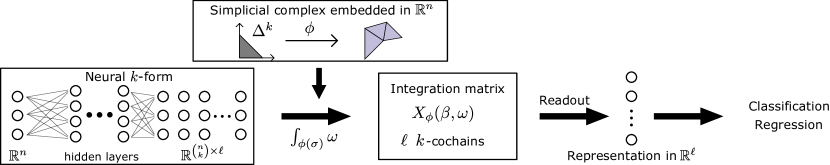
Figure 2: A schematic of our proposed neural $k$-form learning architecture.

Implementation

Our methods can be realised using any deep learning framework that permits training an MLP. We created a proof-of-concept implementation using PyTorch-Geometric (Fey & Lenssen, 2019) and PyTorch-Lightning (Falcon & The PyTorch Lightning team, 2019) and are working on making it available.

5 Experiments and Examples

Synthetic Path Classification

Our first experiment is classifying paths in $\mathbb{R}^{2}$. The goal of the experiment is pedagogical; it illustrates how to interpret the learned $1$-forms rather than benchmark the method. A piecewise linear path in $\mathbb{R}^{n}$ is a simplicial complex determined by an ordered sequence of node embeddings. The $1$-simplices are linear maps $\sigma_{i}:I\to\mathbb{R}^{n}$ from the $i$-th embedded node and to the $(i+1)$-st embedded node, where the full path corresponds to the $1$-chain $\sum_{i}\sigma_{i}$. The integral of this chain against a 1-form corresponds to the path integral. In Figure 3(a) we show three classes of piece-wise linear paths in $\mathbb{R}^{2}$ that we will classify using our method.

The idea is that we will learn three $1$-forms which correspond to each class. To initialise the three $1$-forms in $\mathbb{R}^{2}$, we randomly initialise an MLP $\psi:\mathbb{R}^{2}\to\mathbb{R}^{2\times 3}$. A forward pass consists of two stages: integration of the $1$-simplices in the path against each of the three forms to produce an integration matrix and (2) taking a column sum and applying softmax to produce a distribution over which we perform CrossEntropyLoss. The $i$-th column sum corresponds to a path integral of the path against the $i$-th form; the prediction of a path is thus determined by which feature $1$-form produces the highest path integral. Backpropagation against this loss function thus attempts to modify the $i$-th $1$-form so that it produces a more positive path integral against the paths in class $i$ and more negative otherwise.

In Figure 3(a), we plot the feature $1$-forms as vector fields over their corresponding classes of paths. Note the vector fields are randomly initialised and updated while the paths are the fixed data points. The learned $1$-forms of each class resemble vector fields that roughly reproduce the paths in their class as integral flow lines, and are locally orthogonal or negatively correlated to paths in the other classes. This is a direct result of the objective function, which attempts to maximise the path integral within each class and minimise it for others. In Figure 3(b) we plot the paths as points colored by class, where the coordinates correspond to the path integrals against the three learned $1$-forms. We see a clear separation between the classes, indicating that the representations trivialise the downstream classification task. We also compare the model with a standard MLP in Appendix E.

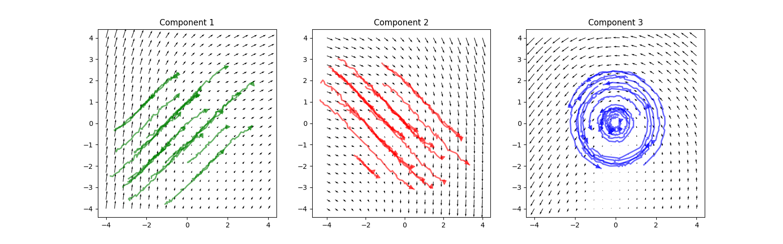
(a) Learned $1$-forms corresponding to paths in each class.

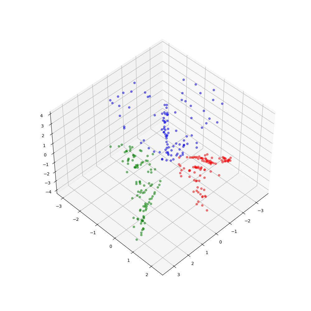
(b) Path Representations.

Figure 3: Synthetic Path Classification via Learnable $1$-forms.

Synthetic Surface Classification

In this example we demonstrate how our framework is of interest to deal with higher dimensional data, i.e. simplicial complexes of dimension $k\geq 2$. Conceptually the difficulty is going from 1-dimensional objects to $k$-dimensional objects with any $k\geq 2$. We restrict ourselves to $k=2$ since higher dimensions are similar to this case. The data we consider here are triangulated surfaces embedded in $\mathbb{R}^{3}$, the underlying combinatorial complex is always the same – a triangulation of a square but the embeddings are different. For a given surface, the embedding of each $2$-simplex is given by linear interpolation between the coordinates of its three vertices in $\mathbb{R}^{3}$. We consider two classes of surfaces, in the first class the embdeddings of the nodes are obtained by sampling along a sinusoidal surface in the $x$-direction and the second class is given by a surface following a sinusoidal shape in the $y$-direction, in each case with added translation and noise.

We use learnable $2$-foms $\omega_{1},\omega_{2}$ on $\mathbb{R}^{3}$ represented by an MLP $\psi:\mathbb{R}^{3}\to\mathbb{R}^{3\times 2}$. In a forward pass of the model we integrate the $2$-forms given by the MLP over the $2$-simplices of a surface. Each point in $\mathbb{R}^{3}$ has a value in $\mathbb{R}^{3\times 2}$ given by the MLP evaluated at that point. The process of integrating over the $2$-simplices corresponds to integrating the point-wise evaluation of the MLP over the regions of $\mathbb{R}^{3}$ defined by each embedded $2$-simplex. This process gives the integration matrix of the forms $\omega_{1},\omega_{2}$ over the $2$-simplices of the complex.

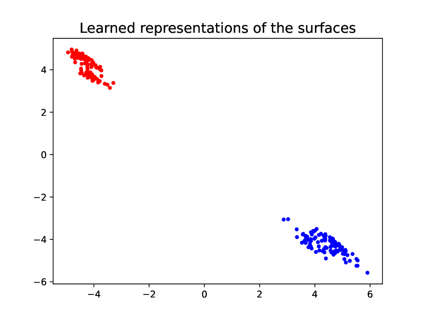
Figure 4: Synthetic surface classification via learnable $2$-forms.

The next step is the readout layer where one sums the entries in each column of the integration matrix, corresponding to summing the value of each cochain over the simplicial complex, giving the total surface integral. As there are two $2$-forms this yields a vector representation in $\mathbb{R}^{2}$, each entry corresponding to a $2$-form. Finally, these representations are then passed through a softmax for classification and CrossEntropyLoss is used as a loss function. The MLP is then updated bybackpropagation.

In Figure 4, we plot the representations in $\mathbb{R}^{2}$ learned through the model described above. Each point represents a surface in the data set and the color is given by the class of the corresponding surface, showing the clear separation learned by the neural $2$-forms. Further details can be found in Appendix E.2.

Table 1: Results (mean accuracy and standard deviation of a $5$-fold cross-validation) on small graph benchmark datasets that exhibit ‘geometrical’ node features. Parameter numbers are approximate because the number of classes differ.

	Params.	BZR	COX2	DHFR	Letter-low	Letter-med	Letter-high
EGNN (Satorras et al., 2021)	1M	$79.51$ p m 1.87	$78.16$ p m 0.46	$64.02$ p m 2.68	$93.20$ p m 0.68	$65.91$ p m 1.60	$68.98$ p m 1.80
GAT (Veličković, 2022)	5K	$81.48$ p m 2.90	$80.73$ p m 2.45	$73.02$ p m 2.54	$90.04$ p m 2.23	$63.69$ p m 5.97	$43.73$ p m 4.13
GCN (Kipf & Welling, 2017)	5K	$79.75$ p m 0.68	$79.88$ p m 1.65	$70.12$ p m 5.43	$81.38$ p m 1.57	$62.00$ p m 2.07	$43.06$ p m 1.67
GIN (Xu et al., 2019)	9K	$79.26$ p m 1.03	$78.38$ p m 0.79	$68.52$ p m 7.38	$85.00$ p m 0.59	$67.07$ p m 2.47	$50.93$ p m 3.47
N$k$F (ours)	4K	$78.77$ p m 0.55	$80.30$ p m 2.42	$64.42$ p m 2.09	$93.42$ p m 1.94	$67.69$ p m 1.28	$62.93$ p m 4.13

Real-World Graphs

In this experiment we attempt to use our model to leverage the geometry of non-equivariant node features in graph classification for a set of benchmark datasets. The basic architecture of the model follows that described in the Architecture and Parameters section. Graphs are represented as a $1$-chain consisting of all their edges. We randomly initialise a set of $\ell$ feature $1$-forms, produce and read-out the integration matrices before feeding through a simple MLP classifer and performing backpropagtion. We use an L2-column readout layer so the network is invariant under edge orientations. Please refer to Section E.3 for specific architectural details. We use state-of-the-art graph neural networks (GNNs) following a recently-described benchmark (Dwivedi et al., 2023), experimenting with different numbers of layers. As an additional comparison partner, we also use a recent equivariant GNN architecture that is specifically geared towards analysing data with an underlying geometry (Satorras et al., 2021).

Table 1 depicts the results on smaller graph datasets in the TU dataset (Morris et al. (2020)) Here the node features that carry both equivariant information (corresponding to 3D coordinates of molecules, for instance) and non-equivariant information (one-hot atomic type, weight etc.). For the non-equivariant models (ours, GCN, GAT) the position features are omitted. Overall, our method exhibits competitive performance, in particular given the fact that it does not make use of any message passing and has a smaller parameter footprint. In Table 2 we compare our model on the larger datasets in the ‘MoleculetNet’ benchmark (Wu et al., 2018). Note that the datasets we have chosen have no provided ’positional’ node features, so the given node features (i.e. atomic weights, valence, etc.) are not equivariant and cannot be compared with EGNN. As LABEL:tab:Benchmarkdatasets_large shows, our model based on neural $k$-forms outperforms state-of-the-art graph neural networks in terms of AUROC, using a fraction of the number of parameters (this also holds for accuracy and average precision, which are, however, not typically reported for these data sets).

Table 2: Results (mean AUROC and standard deviation of $5$ runs) on benchmark datasets from the ‘MoleculeNet’ database (Wu et al., 2018). While the GNNs also train for smaller numbers of parameters, we observed significant drops in predictive performance. We thus report only the best results for GNNs, using the most common models described in the literature.

	Params.	BACE	BBBP	HIV
GAT (Veličković et al., 2018)	135K	$69.52$ p m 17.52	$76.51$ p m 3.36	$56.38$ p m 4.41
GCN (Kipf & Welling, 2017)	133K	$66.79$ p m 1.56	$73.77$ p m 3.30	$68.70$ p m 1.67
GIN (Xu et al., 2019)	282K	$42.91$ p m 18.56	$61.66$ p m 19.47	$55.28$ p m 17.49
N$k$F (ours)	9K	$83.50$ p m 0.55	$86.41$ p m 3.64	$76.70$ p m 2.17

6 Discussion

Summary

We developed neural $k$-forms, a method for learning representations of simplicial cochains to solve tasks on embedded graphs and simplicial complexes. Deviating from the predominant paradigms in geometric deep learning, our method adopts a fundamentally different novel perspective based on integration of forms in the ambient feature space. We have shown the feasibility of the method through a comprehensive experimental suite, demonstrating its effectiveness using only a very small number of parameters. Notably, our method does not utilise any kind of message passing, and we hypothesise that it is possible that this implies that issues like over-smoothing may affect our method less than graph neural networks.

Limitations

A conceptual limitation is that we require (at least) the existence of node or vertex coordinates, i.e. our method only operates on embedded complexes. The computational feasibility of higher order $k$-forms in large embedding spaces is another possible limitation. Indeed, the number of monomial $k$-forms in $\mathbb{R}^{n}$ is $\binom{n}{k}$, and similar issues arise for numerical integration over higher dimensional simplices. Further, we have only benchmarked our method on graph classification tasks. It remains to be seen whether the method performs as well on graph regression tasks, as well as for benchmark learning tasks on higher dimensional simplicial complexes. Finally, our model currently has no scheme for dealing with node features which are equivariant with respect to the embedding space.

Outlook

We aim to study these issues, as well as the behaviour of our methods in the context of long-range dependencies, in a follow-up work. In addition, since our neural $k$-form formulation is equivalent to an MLP, the learning process may benefit from the plethora of existing methods and tricks that are applied to optimise MLPs in practice. We argue that our experiments point towards the utility of using a geometric interpretation of our representations as integrals over $k$-forms may provide valuable insights to practitioners. Lastly, we provide a small example of a Convolutional $1$-form network in Appendix D that may lead to better incorporation of equivariant node embeddings. We provide this auxiliary example as part of a broader future work program of rebuilding common ML architectures on top of neural $k$-forms rather than message passing schemes.

Appendix A Differential Forms in $\mathbb{R}^{n}$ Background

In this section, we provide a basic background in the theory of differential forms. The more complete references see (Lee, 2003) for basic differential geometry, and (Jost, 2017) for Riemannian geometry of $k$-forms. See (Tao, 2009) for a short but illuminating article on the intuition behind differential forms.

Tangent and Cotangent Bundles on $\mathbb{R}^{n}$

In $\mathbb{R}^{n}$, the tangent space $T_{p}(\mathbb{R}^{n})$ at a point $p\in\mathbb{R}^{n}$ is the vector space space spanned by the partial derivatives $\partial/\partial x_{i}(p)$. The cotangent space at $p$ is the linear dual $T^{*}(\mathbb{R}^{n})$ of the tangent space; i.e. the space of linear maps $\mathsf{Hom}_{\mathbb{R}}(T_{p}(\mathbb{R}^{n}),\mathbb{R})$. Note that both spaces are isomorphic to $\mathbb{R}^{n}$. The tangent bundle is the space $T(\mathbb{R}^{n})=\sqcup_{p}T_{p}(\mathbb{R}^{n})$ consisting of gluing all tangent space together, where the topology is induced by the projection map $\pi:T(\mathbb{R}^{n})\to\mathbb{R}^{n}$. Likewise, the cotangent bundle is the space $T^{*}(\mathbb{R}^{n})=\sqcup_{p}T_{p}^{*}(\mathbb{R}^{n})$.

The space of vector fields $\mathfrak{X}(\mathbb{R}^{n})$ over $\mathbb{R}^{n}$ is the space of sections of the tangent bundle; that is, maps $v:\mathbb{R}^{n}\to T_{*}(\mathbb{R}^{n})$ such that $\pi\circ v=id_{\mathbb{R}^{n}}$. Vector fields decompose into the form $\sum_{i}v_{i}(p)\partial/\partial x_{i}(p)$, where $v_{i}:\mathbb{R}^{n}\to\mathbb{R}$. The space of $1$-forms $\Omega^{1}(\mathbb{R}^{n})$ over $\mathbb{R}^{n}$ consists of the sections $\omega:\mathbb{R}^{n}\to T^{*}(\mathbb{R}^{n})$ of the cotangent bundle.

Riemannian Structure on $\mathbb{R}^{n}$

The space $\mathbb{R}^{n}$ is a Riemannian manifold. That is, it has a non-degenerate bilinear form

$$\langle-,-\rangle_{p}:T_{p}(\mathbb{R}^{n})\otimes T_{p}(\mathbb{R}^{n})\to\mathbb{R}.$$ (12)

The inner product is defined on by linear extension of the formula

$$\langle\partial/\partial x_{i}(p),\partial/\partial x_{j}(p)\rangle_{p}=\langle x_{i},x_{j}\rangle$$ (13)

where the second inner product is the standard inner product on $\mathbb{R}^{n}$. Over $\mathbb{R}^{n}$, the spaces of vector fields and $1$-forms are isomorphic via the sharp isomorphism

$$\#:\mathfrak{X}(\mathbb{R}^{n}) \to\Omega^{1}(\mathbb{R}^{n})$$ (14)

$$\sum_{i}v_{i}\partial/\partial x_{i} \mapsto\sum_{i}v_{i}dx_{i}$$ (15)

where $dx_{i}$ is the $1$-form which is locally $dx_{i}(p)=\langle-,\partial/\partial x_{i}(p)\rangle_{p}:T_{p}(\mathbb{R}^{n})\to\mathbb{R}$.

Exterior Products

Let $V$ be a real vector space. Recall that an alternating $k$-covector on $V$ is a map

$$\alpha:\bigotimes_{k}V\to\mathbb{R}$$ (16)

that is alternating with respect to permutations. That is, that

$$\alpha(v_{1},v_{2},\ldots,v_{k})=(-1)^{sgn(\tau)}\alpha(v_{\tau(1)},v_{\tau(2)},\ldots,v_{\tau(k)}).$$ (17)

The $k$-th exterior product $\Lambda^{k}(V^{*})$ over $V$ is the space of alternating $k$-covectors.

$k$-Forms

The $k$-th exterior product of the cotangent bundle $\Lambda^{k}T^{*}(\mathbb{R}^{n})$ is the tensor bundle defined by locally taking the $k$-th exterior product $\Lambda^{k}T^{*}_{p}(\mathbb{R}^{n})$ of each cotangent space. A differential $k$-form $\omega\in\Omega^{k}(\mathbb{R}^{n})$ over a $\mathbb{R}^{n}$ is a smooth section of the $k$-th exterior product of the cotangent bundle $\Lambda^{k}T^{*}M$. The space of forms $\Omega^{*}(\mathbb{R}^{n})$ of any dimension has an algebra structure given by the wedge product. The wedge product is multi-linear and satisfies anti-commutativity

$$dx_{i}\wedge dx_{j}=-dx_{j}\wedge dx_{i}$$ (18)

as well as permutation equivariance

$$dx_{i_{1}}\wedge\ldots\wedge dx_{i_{k}}=(-1)^{sgn(\tau)}dx_{i_{\tau(1)}}\wedge\ldots\wedge dx_{i_{\tau(k)}}$$ (19)

for permutations $\tau$. As described in the body of the paper, $k$-forms have a canonical monomial decomposition given by

$$\omega=\sum_{I}\alpha_{I}dx_{I}.$$ (20)

where $dx_{I}=dx_{i_{1}}\wedge\ldots\wedge dx_{i_{k}}$ for a multi-index $I=(i_{1},\ldots,i_{k})$ and scaling maps $\alpha_{I}:\mathbb{R}^{n}\to\mathbb{R}$.

Types of $k$-forms

Differential $k$-forms are $k$-forms where the scaling maps $\alpha_{I}$ are smooth; this is equivalent to the condition $\omega$ that is a smooth section of $k$-th exterior product of the cotangent bundle. When working with both neural $k$-forms and over non-compact spaces like $\mathbb{R}^{n}$, we often need to define other types of forms.

1. A $k$-form $\omega\in\Omega^{k}_{c}(\mathbb{R}^{n})$ is compactly supported whenever each of the $\alpha_{I}$ are compactly supported.

2. A $k$-form $\omega\in L_{2}\Omega^{k}(\mathbb{R}^{n})$ is $L_{2}$ whenever each $\alpha_{I}$ is square integrable.

3. A $k$-form $\omega\in\Omega^{k}_{PL}(\mathbb{R}^{n})$ is piecewise linear if there exists a triangulation of $\mathbb{R}^{n}$ such that each $\alpha_{I}$ is piece-wise smooth over the triangulation.

Inner Products on $k$-forms

The choice of Riemannian metric on $\mathbb{R}^{n}$ extends to an inner product on the $k$-th exterior product of the cotangent space by

$$\langle-,-\rangle_{p}:\Lambda^{k}T^{*}_{p}(\mathbb{R}^{n})\otimes\Lambda^{k}T^{*}_{p}(\mathbb{R}^{n}) \to\mathbb{R}$$

$$\langle\omega_{1}\wedge\ldots\wedge\omega_{k},\eta_{1}\wedge\ldots\wedge\eta_{k}\rangle_{p} \mapsto\det\langle\omega_{i},\eta_{j}\rangle_{i,j}.$$

where $\omega^{i},\eta_{j}\in\Omega^{1}(\mathbb{R}^{n})$. This induces an inner product over the compactly supported $k$-forms $\Omega_{c}^{k}(M)$ by integration

$$\langle\omega_{1}\wedge\ldots\wedge\omega_{k},\eta_{1}\wedge\ldots\wedge\eta_{k}\rangle=\int_{p\in\mathbb{R}^{n}}\langle\omega_{1}\wedge\ldots\wedge\omega_{k},\eta_{1}\wedge\ldots\wedge\eta_{k}\rangle_{p}\,dVol(\mathbb{R}^{n})$$ (21)

against the volume form $Vol(\mathbb{R}^{n})$ on $\mathbb{R}^{n}$.

Orthonormal Coframes

Equip $\mathbb{R}^{n}$ with the usual Riemannian structure, the compactly supported $k$-forms $\Omega^{k}_{c}(\mathbb{R}^{n})$ with the inner product $\langle-,-\rangle_{\Omega}$ described above and induced norm

$$\lVert\omega\rVert^{2}_{\Omega}=\langle\omega,\omega\rangle_{\Omega}$$

for $\omega\in\Omega^{k}_{c}(\mathbb{R}^{n})$. With this structure, the monomial $k$-forms form an orthornomal coframe in the sense that

$$\langle dx^{I},dx^{I^{\prime}}\rangle_{p}=\begin{cases}1&\text{if }I=I^{\prime}\\ 0&\text{else}\end{cases}$$ (22)

for each $p\in\mathbb{R}^{n}$.

Integration of $k$-forms

Following (Taylor, 2006), we define integration of monomial $k$-forms $\omega=\sum_{I}\alpha_{I}dx_{I}$ then extend via linearity to arbitary $k$-forms. Let $\phi:\Delta^{k}\to\mathbb{R}^{n}$ be a smooth map and coordinatize $\Delta^{k}$ with $(t_{1},t_{2},\ldots,t_{k})$ as above.

The pullback map of $\phi$ is a map $\phi^{*}:\Omega(\mathbb{R}^{n})\to\Omega(\Delta^{k})$ taking forms on $\mathbb{R}^{n}$ to forms on $\Delta^{k}$. In coordinates, the pullback $\phi^{*}\omega\in\Omega^{k}(\Delta^{k})$ of $\omega$ along $\phi$ is defined by the formula

$$\phi^{*}\omega=\sum_{I}\alpha_{I}(\phi^{*}dx_{i_{1}})\wedge(\phi^{*}dx_{i_{2}})\wedge\ldots\wedge(\phi^{*}dx_{i_{k}})$$ (23)

where

$$\phi^{*}dx_{i}=\sum_{j}\dfrac{\partial\phi_{i}}{\partial t_{j}}dt_{j}$$ (24)

and $\phi_{i}$ is the $x_{i}$-component of $\phi$. Note that by the monomial decomposition in Equation 4, the pullback can be written as

$$\phi^{*}\omega=fdt_{1}\wedge dt_{2}\wedge\ldots\wedge dt_{k}$$ (25)

for some smooth function $f:\Delta^{k}\to\mathbb{R}$.

We define the integral $\int_{\phi}$ to be the standard Riemann integral

$$\int_{\phi}\omega:=\int_{\Delta^{k}}fdt_{1}dt_{2}\ldots dt_{k}.$$ (26)

The function $f$ can be computed explicitly by unwinding 23 using the algebraic relations 18 and 19. Namely, for the monomial $k$-form $\omega=\alpha_{I}dx_{I}$ we have

$$\phi^{*}\omega =\alpha_{I}(\phi)\Big{(}\sum_{j}\dfrac{\partial\phi_{i_{1}}}{\partial t_{j}}dt_{j}\Big{)}\wedge\ldots\wedge\Big{(}\sum_{j}\dfrac{\partial\phi_{i_{k}}}{\partial t_{j}}dt_{j}\Big{)}$$ (27)

$$=\alpha_{I}(\phi)\Bigg{(}\sum_{\tau}sgn(\tau)\dfrac{\partial\phi_{i_{1}}}{\partial t_{\tau(1)}}\cdots\dfrac{\partial\phi_{i_{k}}}{\partial t_{\tau(k)}}\Bigg{)}dt_{1}\wedge\ldots\wedge dt_{k}$$ (28)

$$=\alpha_{I}(\phi)\varepsilon^{I}(D\phi)dt_{1}\wedge\ldots\wedge dt_{k}$$ (29)

The above calculation in conjunction with 26 recovers the formula for the integral

$$\int_{\phi}\omega=\sum_{I}\int_{\Delta^{k}}\alpha_{I}(\phi)\varepsilon^{I}(D\phi)dt$$ (30)

of a general $k$-form $\omega$ given in 5.

Remark 9.

In the special case that $\phi$ is an affine map, then the Jacobian is expressed as

$$D\phi_{i,j}=\Big{[}\phi^{i}(t_{j})-\phi^{i}(t_{0})\Big{]}_{i,j}$$

Properties of Integration

Throughout the paper, we refer to the linearity and orientation equivariance of integration of forms over simplices. These are a consequence of the following theorem.

Proposition 10 ((Lee, 2003), 16.21).

Suppose $M$ is an $n$-manifold with corners and $\omega,\eta\in\Omega^{n}(M)$ are smooth $n$-forms. Then

1. For $a,b\in\mathbb{R}$ we have

   $$\int_{M}a\omega+b\eta=a\int_{M}\omega+b\int_{M}\eta$$

2. Let $-M$ denote $M$ with the opposite orientation. Then

   $$\int_{-M}\omega=-\int_{M}\omega.$$

Appendix B Integration of $k$-forms in Practice

We give further practical details on how to approximate integrals in the case of $2$-forms. For more detailed and accessible introductions we recommend the following references (Taylor, 2006; Tao, 2009).

Explicit computations for $2$-forms

In Section 5 we use integration of $2$-forms on $2$-dimensional simplicial complexes in order to classify surfaces. We will derive an explicit method to approximate the integral of $2$-forms in $\mathbb{R}^{n}$ over an embedded $2$-simplex based on the theory above.

Recall that a $2$-form $\omega\in\Omega^{2}(\mathbb{R}^{n})$ can be written in coordinates as

$$\omega=\sum_{0\leq i<j\leq n}\alpha_{i,j}dx_{i}\wedge dx_{j},$$ (31)

where $\alpha_{i,j}:\mathbb{R}^{n}\longrightarrow\mathbb{R}$ are smooth maps. We consider a map $\phi:\Delta^{2}\longrightarrow\mathbb{R}^{n}$ giving the embedding of the standard $2$ simplex in $\mathbb{R}^{n}$. Using the expression from Equation 26:

$$\int_{\phi(\Delta^{2})}\omega=\int_{\Delta^{2}}\phi^{*}(\omega)$$

we will show how to integrate $\omega$ on the embedded simplex $\phi(\Delta^{2})$.

Using local coordinates to express the embedding $\phi(t_{1},t_{2})=(x_{1},\dots,x_{n})$ we can write out explicitly the pullback of a $2$-form $\omega\in\Omega^{2}(\mathbb{R}^{n})$ via the map $\phi$:

$$\phi^{*}\big{(}\sum_{0\leq i<j\leq n}\alpha_{i,j}dx_{i}\wedge dx_{j}\big{)}=\sum_{0\leq i<j\leq n}\big{(}\alpha_{i,j}\circ\phi\big{)}\big{(}\frac{\partial x_{i}}{\partial t_{1}}dt_{1}+\frac{\partial x_{i}}{\partial t_{2}}dt_{2}\big{)}\wedge\big{(}\frac{\partial x_{j}}{\partial y_{1}}dt_{1}+\frac{\partial x_{j}}{\partial t_{2}}dt_{2}\big{)}$$

$$=\sum_{0\leq i<j\leq n}\big{(}\alpha_{i,j}\circ\phi\big{)}\Big{(}\big{(}\frac{\partial x_{i}}{\partial t_{1}}dt_{1}\wedge\frac{\partial x_{j}}{\partial t_{2}}dt_{2}\big{)}+\big{(}\frac{\partial x_{i}}{\partial t_{2}}dt_{2}\wedge\frac{\partial x_{j}}{\partial t_{1}}dt_{1}\big{)}\Big{)}$$

$$=\sum_{0\leq i<j\leq n}\big{(}\alpha_{i,j}\circ\phi\big{)}\Big{(}\underbrace{\frac{\partial x_{i}}{\partial t_{1}}\frac{\partial x_{j}}{\partial t_{2}}-\frac{\partial x_{i}}{\partial t_{2}}\frac{\partial x_{j}}{\partial t_{1}}}_{A}\Big{)}dt_{1}\wedge dt_{2}$$ (32)

In the computational context that we consider we want to integrate a $2$-form on the $2$-simplices of a complex embedded in $\mathbb{R}^{n}$. We set some notation here, each $2$-simplex $\sigma\in X$ is the image of an affine map $\phi(t)=\Phi t+b:\Delta^{2}\longrightarrow\mathbb{R}^{n}$, where $\Phi=D\phi=[\phi_{i,1},\phi_{i,2}]_{0\leq i\leq n}$ is a $(n\times 2)$-matrix. Since $\phi$ is an affine map the term $A$ in 32 becomes

$$A=\varepsilon^{(i,j)}(D\phi)=\det\Phi_{i}^{j},$$ (33)

with $\Phi_{i}^{j}$ denoting the $(2\times 2)-$submatrix of $\Phi$ corresponding to the rows $i$ and $j$.

Putting all this together we obtain:

$$\phi^{*}(\omega)=\sum_{0\leq i<j\leq n}\alpha_{i,j}(\phi)\det\Phi_{i}^{j}dt_{1}\wedge dt_{2}.$$ (34)

So the integration becomes

$$\int_{\phi(\Delta^{2})}\omega=\int_{\Delta^{2}}\phi^{*}(\omega)=\int_{\Delta^{2}}\underbrace{\sum_{0\leq i<j\leq n}\alpha_{i,j}(\phi)\det\Phi_{i}^{j}}_{g}dt_{1}\wedge dt_{2}.$$ (35)

Computationally we cannot perform exact integration of $2$-forms so in practise we approximate the integral on $\Delta^{2}$ above by a finite sum, as is done with Riemann sums in the classical case. To do so the first step is to subdivide the domain of integration $\Delta^{2}$ into a collection $\mathcal{S}$ of smaller simplices with vertices denoted by $v$. Then the integral is approximated by summing the average value of the map $g$ on each simplex of the subdivision:

$$\int_{\Delta^{2}}gdt_{1}\wedge dt_{2}\approx\sum_{s\in\mathcal{S}^{2}}\frac{1}{3}\sum_{v\in s}g(v)\cdot vol(s).$$ (36)

An explicit method of this sort can be easily generalized to higher dimensional simplices in order to compute integrals of $k$-forms on $k$-dimensional simplicial complexes.

Appendix C Proofs

Universal Approximation I

We start with the proof of Proposition 3. First, recall the well-known following universal approximation theorem for neural networks. We cite here a version appearing in (Pinkus, 1999).

Theorem 11 (Universal Approximation Theorem, Thm 3.1 (Pinkus, 1999)).

Let $\sigma\in C(\mathbb{R},\mathbb{R})$ be a non-polynomial activation function. For every $n,\ell\in\mathbb{N}$, compact subset $K\subset\mathbb{R}^{n}$, function $f\in C(K,\mathbb{R}^{\ell})$ and $\epsilon>0$ there exists:

• an integer $j\in\mathbb{N}$;

• a matrix $W_{1}\in\mathbb{R}^{j\times n}$;

• a bias vector $b\in\mathbb{R}^{j}$ and

• a matrix $W_{2}\in\mathbb{R}^{\ell\times j}$

such that

$$\lVert f-g\rVert_{\infty}<\varepsilon$$

where $g$ is the single hidden layer MLP

$$g(x)=W_{2}\sigma(W_{1}x+b).$$

Theorem 3.

Let $\alpha\in C(\mathbb{R},\mathbb{R})$ be a non-polynomial activation function. For every $n\in\mathbb{N}$ and compactly supported $k$-form $\eta\in\Omega^{k}_{c}(\mathbb{R}^{n})$ and $\epsilon>0$ there exists a neural $k$-form $\omega^{\psi}$ with one hidden layer such that

$$\lVert\omega^{\psi}-\eta\rVert_{\Omega}<\epsilon.$$

Proof.

Denote the scaling functions of $\eta$ by

$$\eta=\sum\eta_{I}dx_{I}.$$

Since $\eta$ is compactly supported, each $\eta_{I}$ is compactly supported over some domain $D$. By 11, for any $\varepsilon>0$ there exists a one layer MLP $\psi:\mathbb{R}^{n}\to\mathbb{R}^{\binom{n}{k}}$ such that

$$\lVert\psi-\bigoplus_{I}\eta_{I}\rVert_{\infty}<\varepsilon/Vol(D)^{1/2}.$$

Using the orthogonality form Equation 22, we have that

$$\lVert\omega^{\psi}-\eta\rVert^{2}_{p}=\langle\omega^{\psi}-\eta,\omega^{\psi}-\eta\rangle_{p}=\sum_{I}(\psi_{I}(p)-\eta_{I}(p))^{2}=\lVert\psi(p)-\oplus_{I}\eta_{I}(p)\rVert_{\mathbb{R}^{\binom{n}{k}}}^{2}\leq\varepsilon^{2}/Vol(D).$$

Integrating the above, we attain

$$\lVert\omega^{\psi}-\eta\rVert^{2}_{\Omega} \leq\int_{D}\langle\omega^{\psi}-\eta,\omega^{\psi}-\eta\rangle_{p}dVol(\mathbb{R}^{n})$$

$$<\varepsilon^{2}/Vol(D)\int_{D}dVol(\mathbb{R}^{n})$$

$$=\varepsilon^{2}$$

proving the result. ∎

Equivariance

Integration is linear in both $k$-forms (Lee (2003), 16.21) and embedded simplicial chains 7 in the sense that it defines a bilinear pairing

$$\int:C_{k}^{sing}(\mathcal{S};\mathbb{R})\otimes\Omega^{k}(\mathbb{R}^{n})\to\mathbb{R}$$ (37)

for some embedded simplicial complex $\phi:\mathcal{S}\to\mathbb{R}^{n}$. This property directly implies the kind of multi-linearity described in Proposition 6. We present a proof here for completeness.

Proposition 6 (Multi-linearity).

Let $\phi:\mathcal{S}\to\mathbb{R}^{n}$ be an embedded simplicial complex. For any matrices $L\in M^{m^{\prime}\times m}(\mathbb{R})$ and $R\in M^{\ell\times\ell^{\prime}}(\mathbb{R})$ we have

$$X_{\phi}(L\beta,\omega R)=LX_{\phi}(\beta,\omega)R$$ (38)

Proof.

On the left we have

$$X_{\phi}(L\beta,\omega)_{i,j} =X\Big{(}\sum_{k}L_{1,k}\beta_{k},\ldots,\sum_{k}L_{m^{\prime},k}\beta_{k},\omega\Big{)}_{i,j}$$ (39)

$$=\int_{\sum_{k}L_{i,k}\beta_{k}}\omega_{j}$$ (40)

$$=\sum_{k}L_{i,k}\int_{\beta_{k}}\omega_{j}$$ (41)

$$=\Big{[}LX_{\phi}(\beta,\omega)\Big{]}_{i,j}.$$ (42)

Similarly, on the right we have

$$X_{\phi}(\beta,\omega R)_{i,j} =X_{\phi}(\beta,\sum_{k}R_{k,1}\omega_{k},\ldots,\sum_{k}R_{k,\ell^{\prime}}\omega_{k}\Big{)}_{i,j}$$ (43)

$$=\int_{\beta_{i}}\sum R_{k,j}\omega_{k}$$ (44)

$$=\sum_{k}R_{k,j}\int_{\beta_{i}}\omega_{k}$$ (45)

$$=\Big{[}X_{\phi}(\beta,\omega)R\Big{]}_{i,j}$$ (46)

∎

Appendix D Additional Experiments

D.1 Convolutional $1$-form Networks

Convolution and Equivariance

Beyond orientation and permuation equivariance, the node embeddings themselves may be equivariant with respect to a group action on the feature space. The class of geometric graph neural networks Han et al. (2022) were designed specifically to deal with such equivariances. The lesson from image processing is that translation equivariance can be mitigated via convolution. In this paradigm processing embedded (oriented) graphs with learnable, ‘template’ $1$-forms is directly analogous to processing images with learnable convolutional filters. To make this connection precise, we will perform a small example to classify oriented graphs.

Synthetic Data

In Figure 5, there are two classes of cycle and star graphs. The cycle graphs have clockwise orientation and the star graph are oriented so edges point inwards. Each data-point is a simplicial complex representing the disjoint union of either three cycle or star graphs which are randomly recentered around the unit square. The chains on each complex are initialised using the standard oriented $1$-simplices as a basis.

Architecture

We initialise a neural network $\psi:\mathbb{R}^{2}\to\mathbb{R}^{2\times 2}$ with a single 64-dimensional hidden layer and ReLU activation which corresponds to two feature $1$-forms. To perform a convolutional pass, we first discretize the unit square to produce a set of translations. At each translation, we restrict the embedded graph to the subgraph within a neighbourhood and weight it by the local node density approximated by a standard kernel density estimator. This is equivalent to translating the $1$-form by the corresponding (negative) vector in $\mathbb{R}^{2}$ and integrating over a small neighbourhood (whose area is a hyperparameter). Integration produces an integration matrix at each point with two columns, and taking the column sum represents the oriented integral of the two convolutional filters against the local neighbourhood of the oriented graph. CrossEntropyLoss is calculated by summing the integrals over all translations and applying softmax.

Interpreting the Results

The integrals are shown in Figure 5 as a colouring of each point in the grid of translations. We plot the learned ’template’ 1-forms next to an example of their respective classes. By the construction of the objective function, the algorithm is trying to maximise the sum of the integrals across all translations within the class. As in the synthetic paths example, the learned filters successfully capture the interpretable, locally relevant structure; the edges in each class resemble flow-lines of the learned vector field in different local neighbourhoods around the relevant translations.

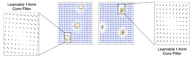
Figure 5: A convolutional $1$-form network with the learned convolutional filters forms.

D.2 Visualising Simplicial Laplacian $1$-Eigenvectors

In this example, we show how we can use neural $1$-form to visualise the $1$-eigenvectors of the simplicial Laplacian of a Rips complex in $\mathbb{R}^{2}$ (Figure 6). The idea is that we start with a collection of eigenvectors of simplicial $1$-cochains, and learn $1$-forms which integrate to them. We see the results in Figure 6(b), where the three eigenvectors belong to the harmonic, gradient-like and curl components of the simplicial Hodge decomposition respectively.

First we generate a point cloud in $\mathbb{R}^{2}$ as a noisey approximation of a circle, then take the Rips complex for a fixed parameter $\varepsilon$. We then calculate the first $9$ eigenvectors of the $1$-simplicial Laplacian, sorted by increasing eigenvalue, and store them as columns of a matrix $Y$ with respect to the standard basis $\beta$. We initialise $9$ neural $1$-forms

$$\omega=(\omega_{1},\omega_{2},\ldots,\omega_{9})\in\bigoplus_{\ell}\Omega^{1}_{PL}(\mathbb{R}^{2})$$

on $\mathbb{R}^{2}$ using a ReLU activation function. Our loss function is then

$$\mathcal{L}(\omega)=\lVert X_{\phi}(\beta,\omega)-Y\rVert$$

where the norm is the standard matrix norm, and $X_{\phi}(\beta,\omega)$ is the evaluation matrix yielded from integrating $\omega$ over $\beta$. When $\mathcal{L}$ is small, the $1$-forms over $\mathbb{R}^{2}$ will correspond to the selected simplicial eigenvectors when integrated over the complex.

Figure 6 shows the results—one notes that the different $1$-forms appear to coalesce around geometric features in the underlying point cloud. Additionally, it is important to observe that the Laplacian $1$-eigenvectors can be categorized into three distinct classes depending on their membership within the components of the Hodge decomposition:

1. The first class consists of eigenvectors that belong to the image of the adjoint of the differential operator $d^{1}$,

2. The second class comprises eigenvectors that reside within the kernel of the Laplacian operator $\Delta^{1}$,

3. Lastly, the third class includes eigenvectors that are part of the image of the differential operator $d^{0}$.

These classes correspond, in the context of simplicial structures, to analogues of rotational, harmonic, and gradient-like vector fields found in Riemannian manifolds. By referring to Fig. 6(b), one can visually identify the class to which each eigenvector belongs based on whether or not there exists rotational structure. We have color-coded these as green, red, and blue, respectively.

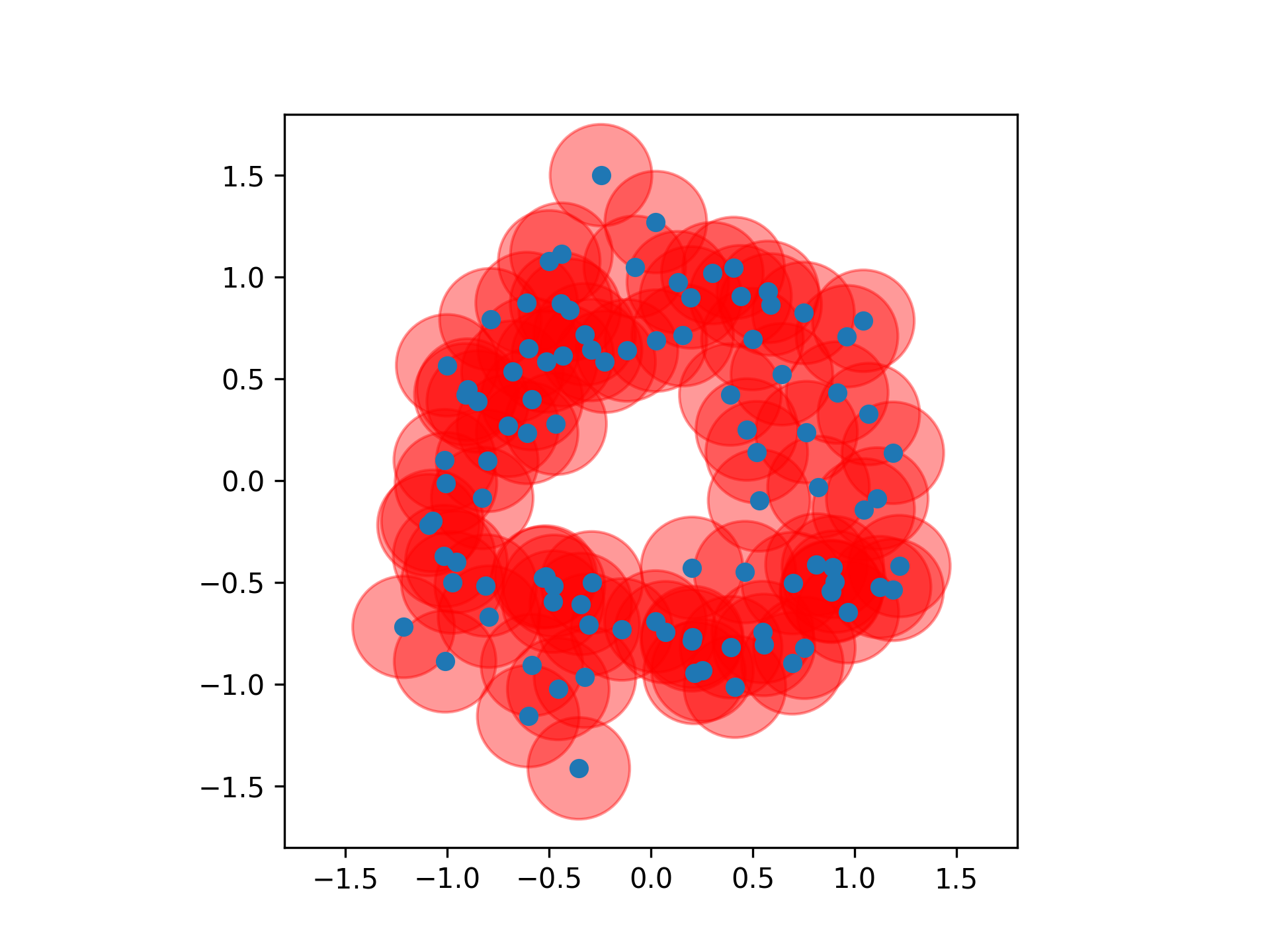
(a) Čech Cover

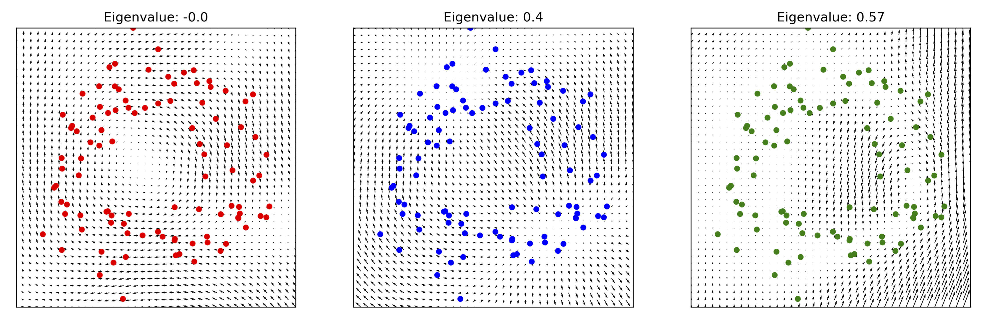
(b) Learned $1$-forms

Figure 6: Approximating the $1$-eigenvectors of the simplicial Laplacian with learnable $1$-forms using the Čech Cover of a point cloud.

Appendix E Experimental Setup and Implementation Details

E.1 Synthetic Path Classification

Synthetic Path Classification

We initialise neural $1$-forms $\omega_{1},\omega_{2},\omega_{3}\in\Omega^{1}_{PL}(\mathbb{R}^{2})$ with ReLU activation for each of the three classes. Each path $p$ is represented as an oriented simplicial complex, where the orientation is induced by the direction of the path. Letting $\beta$ be the standard basis, the three $1$-forms generate an evaluation matrix $X_{\phi}(\beta,\omega)$ whose entries are the integration of the $1$-form $\int_{e_{i}}\omega_{j}$ against each $1$-simplex in the paths.

The readout function sums the entries in each column, which by the linearity of integration, represents the path integral along $p$ against each $\omega_{i}$. In short, each path $p$ is represented as a vector in $\mathbb{R}^{3}$ using the map

$$p\mapsto(\int_{p}\omega_{1},\int_{p}\omega_{2},\int_{p}\omega_{3})\in\mathbb{R}^{3}.$$ (47)

We then use cross-entropy loss between this vector and the class vector. In this design, each $1$-form corresponds to a class, and a path should ideally have a high path integral against this form if and only if it belongs to the class.

Comparison with Neural Networks. In our synthetic experiment, we test whether edge data is necessary by examining whether we can attain comparable results using only the embedded vertices of the path.

In our context, the right framework to analyse the vertices is a set of $0$-forms on $\mathbb{R}^{2}$ - in other words, scalar functions over $\mathbb{R}^{2}$. We use the same setup as before, where we initialise three functions $f_{1},f_{2},f_{3}\in\Omega_{PL}^{0}(\mathbb{R}^{2})$ corresponding to the three classes. Integration of the vertices in the path against each of $f_{i}$ simply corresponds to evaluating $f_{i}$ at the vertex. Summing the columns of the evaluation matrix then sums up the value of $f_{i}$ at all points in a path. In this sense, each $f_{i}$ functions much like an approximated ’density’ for the vertices of each class - albeit with negative values.

In Figure 7, we show example paths from each class against the learned scalar function representing that class. In this example, the vertices of paths in each class have a similar density. One sees that the algorithm learns something reasonable, picking out minor fluctuations in density, but struggles overall to separate out the classes. With the same number of parameters and training time, the algorithm is only able to achieve a training accuracy of 37%.

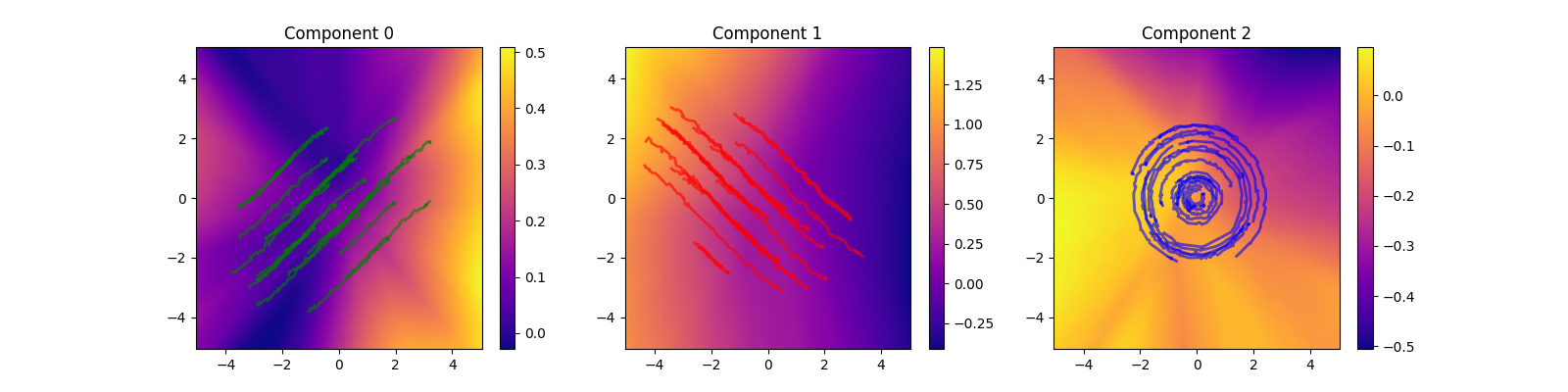
Figure 7: Learned $0$-forms for Synthetic Path Classifcation.

E.2 Synthetic Surface Classification

We consider two classes of synthetic surfaces obtained by embedding a triangulated square in $\mathbb{R}^{3}$. The embedding of the vertices of the triangulated square are given by functions of the type $\phi_{1}(x,y)=sin(x)+\epsilon(x,y)$ for the first class and $\phi_{2}(x,y)=sin(y)+\epsilon(x,y)$ for the second class, where $\epsilon$ is random noise. We initialise two neural $2$-forms $\omega_{1},\omega_{2}\in\Omega^{2}_{PL}(\mathbb{R}^{3})$ with ReLU activation for each of the classes. Letting $\beta$ be the standard basis, the two $2$-forms generate an evaluation matrix $X_{\phi}(\beta,\omega)$ whose entries are the integration of the $2$-form $\int_{e_{i}}\omega_{j}$ against each $2$-simplex in the surfaces. The readout function sums the entries in each column, which represents the integral of each $\omega_{i}$ over the entire surface, thus yielding a representation of the surfaces in $\mathbb{R}^{2}$ in the following way

$$s\mapsto(\int_{s}\omega_{1},\int_{s}\omega_{2},)\in\mathbb{R}^{2}.$$ (48)

Finally, we use the cross entropy loss function to classify the surfaces into the two classes. In this design, each $2$-form corresponds to a class, and a surface should ideally have a high integral against this form if and only if it belongs to the class.

Figure 8 shows the integral of $\omega_{1}$ on surfaces taken from each of the two classes. This integral is positive for elements of the first class and negative for elements of the second class. Similarly the values for the integral of $\omega_{2}$ is negative on surfaces of the first class and positive on elements of the second class.

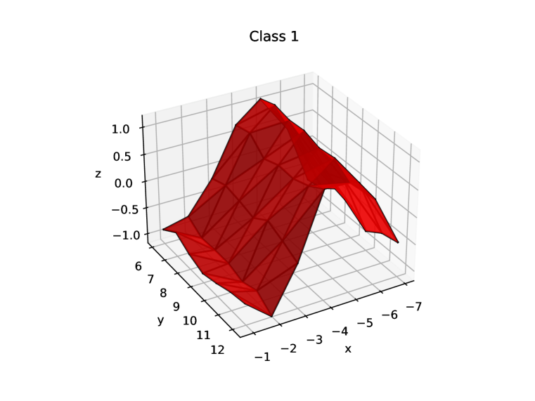
(a) Integral of $\omega_{1}$ on a representative of the first class.

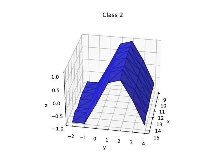
(b) Integral of $\omega_{1}$ on a representative of the first class.

Figure 8: Representative surfaces of each classes, colored by the integral of the learned $2$-form $\omega_{1}$ over the surface. The integral of $\omega_{1}$ over elements of the first class yields positive values whereas the integral of the same form over elements of the second class yields negative values. For the form $\omega_{2}$ the opposite is true.

E.3 Graph Benchmark Datasets

For the small graph benchmark datasets (AIDS, BZR, COX2, DHFR, Letter-low, Letter-med, Letter-high), we use a learning rate of $1e-3$, a batch size of $16$, a hidden dimension of $16$, and $h=5$ discretisation steps for all $k$-forms. For our comparison partners, i.e. for the graph neural networks, we use $h$ hidden layers to permit message passing, followed by additive pooling. As a result, all models have roughly equivalent parameter budgets, with our model having access to the smallest number of parameters.

Architectures.

Our model architectures for our comparison partners follow the implementations described in the respective papers (Kipf & Welling, 2017; Veličković et al., 2018; Xu et al., 2019). We make use of the pytorch-geometric package and use the classes GAT, GCN, and GIN, respectively. Our own model consists of a learnable vector field and a classifier network. Letting $H$ refer to the hidden dimension and $D_{\text{in}}$, $D_{\text{out}}$ to the input/output dimension, respectively, we realise the vector field as an MLP of the form Linear[$D_{\text{in}}$,$H$] - ReLU - Linear[$H$,$H/2$] - ReLU - Linear[$H/2$,$D_{\text{out}}$]. The classifier network consists of another MLP, making use the number of steps $h$ for the discretisation of our cochains. It has an architecture of Linear[$h$,$H$] - ReLU - Linear[$H$,$H/2$] - ReLU - Linear[$H/2$,$c$], where $c$ refers to the number of classes.

Training.

We train all models in the same framework, allocating at most $100$ epochs for the training. We also add early stopping based on the validation loss with a patience of $40$ epochs. Moreover, we use a learning rate scheduler to reduce the learning rate upon a plateau.

References

- Barbero et al. (2022) Federico Barbero, Cristian Bodnar, Haitz Sáez de Ocáriz Borde, Michael Bronstein, Petar Veličković, and Pietro Liò. Sheaf Neural Networks with Connection Laplacians, 2022. URL https://arxiv.org/abs/2206.08702.
- Bodnar et al. (2021a) Cristian Bodnar, Fabrizio Frasca, Nina Otter, Yu Guang Wang, Pietro Liò, Guido Montufar, and Michael M. Bronstein. Weisfeiler and lehman go cellular: CW networks. In Advances in Neural Information Processing Systems, 2021a. URL https://openreview.net/forum?id=uVPZCMVtsSG.
- Bodnar et al. (2021b) Cristian Bodnar, Fabrizio Frasca, Yu Guang Wang, Nina Otter, Guido Montúfar, P. Liò, and M. Bronstein. Weisfeiler and Lehman go Topological: Message Passing Simplicial Networks. Proceedings of the 38th International Conference on Machine Learning PMLR, 139:1026–1037, 2021b.
- Bronstein et al. (2017) Michael M. Bronstein, Joan Bruna, Yann LeCun, Arthur Szlam, and Pierre Vandergheynst. Geometric deep learning: Going beyond Euclidean data. IEEE Signal Processing Magazine, 34(4):18–42, 2017. doi: 10.1109/MSP.2017.2693418.
- Bunch et al. (2020) Eric Bunch, Qian You, Glenn Fung, and Vikas Singh. Simplicial 2-complex convolutional neural nets, 2020. URL https://arxiv.org/abs/2012.06010.
- Cybenko (1989) G. Cybenko. Approximation by superpositions of a sigmoidal function. Mathematics of Control, Signals, and Systems, 2(4):303–314, 1989. doi: 10.1007/bf02551274.
- Dwivedi et al. (2023) Vijay Prakash Dwivedi, Chaitanya K. Joshi, Anh Tuan Luu, Thomas Laurent, Yoshua Bengio, and Xavier Bresson. Benchmarking Graph Neural Networks. Journal of Machine Learning Research, 24(43):1–48, 2023.
- Ebli et al. (2020) Stefania Ebli, Michaël Defferrard, and Gard Spreemann. Simplicial Neural Networks. In Topological Data Analysis and Beyond workshop at NeurIPS, 2020. URL https://arxiv.org/abs/2010.03633.
- Falcon & The PyTorch Lightning team (2019) William Falcon and The PyTorch Lightning team. PyTorch Lightning, March 2019. URL https://github.com/Lightning-AI/lightning.
- Fey & Lenssen (2019) Matthias Fey and Jan Eric Lenssen. Fast Graph Representation Learning with PyTorch Geometric, May 2019. URL https://github.com/pyg-team/pytorch_geometric.
- Gasteiger et al. (2019) Johannes Gasteiger, Stefan Weiß enberger, and Stephan Günnemann. Diffusion improves graph learning. In H. Wallach, H. Larochelle, A. Beygelzimer, F. d'Alché-Buc, E. Fox, and R. Garnett (eds.), Advances in Neural Information Processing Systems, volume 32. Curran Associates, Inc., 2019.
- Giusti et al. (2022) L. Giusti, C. Battiloro, P. Di Lorenzo, S. Sardellitti, and S. Barbarossa. Simplicial Attention Neural Networks, 2022. URL https://arxiv.org/abs/2203.07485.
- Goh et al. (2022) Christopher Wei Jin Goh, Cristian Bodnar, and Pietro Liò. Simplicial Attention Networks, 2022. URL https://arxiv.org/abs/2204.09455.
- Hacker (2020) Celia Hacker. k-simplex2vec: a simplicial extension of node2vec. In Topological Data Analysis and Beyond workshop at NeurIPS, 2020. URL https://arxiv.org/abs/2010.05636.
- Hajij et al. (2020) Mustafa Hajij, Kyle Istvan, and Ghada Zamzmi. Cell Complex Neural Networks. CoRR, abs/2010.00743, 2020. URL https://arxiv.org/abs/2010.00743.
- Hajij et al. (2023) Mustafa Hajij, Ghada Zamzmi, Theodore Papamarkou, Nina Miolane, Aldo Guzmán-Sáenz, Karthikeyan Natesan Ramamurthy, Tolga Birdal, Tamal K. Dey, Soham Mukherjee, Shreyas N. Samaga, Neal Livesay, Robin Walters, Paul Rosen, and Michael T. Schaub. Topological Deep Learning: Going Beyond Graph Data, 2023. URL https://arxiv.org/abs/2206.00606.
- Han et al. (2022) Jiaqi Han, Yu Rong, Tingyang Xu, and Wenbing Huang. Geometrically equivariant graph neural networks: A survey, 2022.
- Hansen & Gebhart (2019) Jakob Hansen and Thomas Gebhart. Sheaf Neural Networks. CoRR, 2019. URL https://arxiv.org/abs/2012.06333.
- Hensel et al. (2021) Felix Hensel, Michael Moor, and Bastian Rieck. A survey of Topological Machine Learning Methods. Frontiers in Artificial Intelligence, 4, 2021. doi: 10.3389/frai.2021.681108. URL https://www.frontiersin.org/articles/10.3389/frai.2021.681108.
- Heydari & Livi (2022) Sajjad Heydari and Lorenzo Livi. Message Passing Neural Networks for Hypergraphs. In Elias Pimenidis, Plamen Angelov, Chrisina Jayne, Antonios Papaleonidas, and Mehmet Aydin (eds.), Artificial Neural Networks and Machine Learning – ICANN 2022, pp. 583–592, Cham, Switzerland, 2022. Springer.
- Horn et al. (2022) Max Horn, Edward De Brouwer, Michael Moor, Yves Moreau, Bastian Rieck, and Karsten Borgwardt. Topological Graph Neural Networks. In International Conference on Learning Representations (ICLR), 2022. URL https://openreview.net/forum?id=oxxUMeFwEHd.
- Hornik et al. (1989) Kurt Hornik, Maxwell Stinchcombe, and Halbert White. Multilayer feedforward networks are universal approximators. Neural Networks, 2(5):359–366, 1989. doi: 10.1016/0893-6080(89)90020-8.
- Jost (2017) Jürgen Jost. Riemannian Geometry and Geometric Analysis. Universitext. Springer, 2017. ISBN 978-3-319-61859-3. doi: 10.1007/978-3-319-61860-9.
- Keros et al. (2022) Alexandros D Keros, Vidit Nanda, and Kartic Subr. Dist2Cycle: A simplicial neural network for homology localization. Proceedings of the AAAI Conference on Artificial Intelligence, 36(7):7133–7142, 2022. doi: 10.1609/aaai.v36i7.20673.
- Kipf & Welling (2017) Thomas N. Kipf and Max Welling. Semi-Supervised Classification with Graph Convolutional Networks. In International Conference on Learning Representations, 2017. URL https://openreview.net/forum?id=SJU4ayYgl.
- Lee (2003) John M. Lee. Introduction to Smooth Manifolds, volume 218 of Graduate Texts in Mathematics. Springer New York, New York, NY, 2003. doi: 10.1007/978-0-387-21752-9.
- Morris et al. (2020) Christopher Morris, Nils M. Kriege, Franka Bause, Kristian Kersting, Petra Mutzel, and Marion Neumann. Tudataset: A collection of benchmark datasets for learning with graphs. In ICML 2020 Workshop on Graph Representation Learning and Beyond (GRL+ 2020), 2020. URL www.graphlearning.io.
- Nanda (2021) Vidit Nanda. Lecture notes in computational algebraic topology, February 2021.
- Nguyen et al. (2023) Khang Nguyen, Nong Minh Hieu, Vinh Duc Nguyen, Nhat Ho, Stanley Osher, and Tan Minh Nguyen. Revisiting over-smoothing and over-squashing using Ollivier–Ricci curvature. In Andreas Krause, Emma Brunskill, Kyunghyun Cho, Barbara Engelhardt, Sivan Sabato, and Jonathan Scarlett (eds.), Proceedings of the 40th International Conference on Machine Learning (ICML), number 202 in Proceedings of Machine Learning Research, pp. 25956–25979. PMLR, 2023.
- Pinkus (1999) Allan Pinkus. Approximation theory of the MLP model in neural networks. Acta Numerica, 8:143–195, 1999. doi: 10.1017/S0962492900002919.
- Roddenberry et al. (2021) T. Mitchell Roddenberry, Nicholas Glaze, and Santiago Segarra. Principled simplicial neural networks for trajectory prediction. CoRR, 2021. doi: 10.48550/ARXIV.2102.10058. URL https://arxiv.org/abs/2102.10058.
- Satorras et al. (2021) Víctor Garcia Satorras, Emiel Hoogeboom, and Max Welling. E(n) equivariant graph neural networks. In Marina Meila and Tong Zhang (eds.), Proceedings of the 38th International Conference on Machine Learning, volume 139 of Proceedings of Machine Learning Research, pp. 9323–9332. PMLR, 2021.
- Tao (2009) Terence Tao. Iii.16 differential forms and integration. In Timothy Gowers, June Barrow-Green, and Imre Leader (eds.), The Princeton Companion to Mathematics, pp. 175–180. Princeton University Press, Princeton, 2009. doi: 10.1515/9781400830398.175.
- Taylor (2006) M.E. Taylor. Measure Theory and Integration. Graduate studies in mathematics. American Mathematical Society, 2006. ISBN 9780821841808. URL https://books.google.de/books?id=AwUPCgAAQBAJ.
- Topping et al. (2022) Jake Topping, Francesco Di Giovanni, Benjamin Paul Chamberlain, Xiaowen Dong, and Michael M. Bronstein. Understanding over-squashing and bottlenecks on graphs via curvature. In International Conference on Learning Representations, 2022. URL https://openreview.net/forum?id=7UmjRGzp-A.
- Veličković (2022) Petar Veličković. Message passing all the way up, 2022.
- Veličković (2023) Petar Veličković. Everything is connected: Graph neural networks. Current Opinion in Structural Biology, 79:102538, 2023. doi: 10.1016/j.sbi.2023.102538.
- Veličković et al. (2018) Petar Veličković, Guillem Cucurull, Arantxa Casanova, Adriana Romero, Pietro Liò, and Yoshua Bengio. Graph attention networks. In International Conference on Learning Representations, 2018. URL https://openreview.net/forum?id=rJXMpikCZ.
- Wu et al. (2018) Zhenqin Wu, Bharath Ramsundar, Evan N. Feinberg, Joseph Gomes, Caleb Geniesse, Aneesh S. Pappu, Karl Leswing, and Vijay Pande. Moleculenet: A benchmark for molecular machine learning. Chemical Science, 9:513–530, 2018. doi: 10.1039/C7SC02664A.
- Xu et al. (2019) Keyulu Xu, Weihua Hu, Jure Leskovec, and Stefanie Jegelka. How Powerful are Graph Neural Networks? In International Conference on Learning Representations, 2019. URL https://openreview.net/forum?id=ryGs6iA5Km.