A shooting-Newton procedure for solving fractional terminal value problems

Abstract

In this paper we consider the numerical solution of fractional terminal value problems: namely, terminal value problems for fractional differential equations. In particular, the proposed method uses a Newton-type iteration which is particularly efficient when coupled with a recently-introduced step-by-step procedure for solving fractional initial value problems, i.e., initial value problems for fractional differential equations. As a result, the method is able to produce spectrally accurate solutions of fractional terminal value problems. Some numerical tests are reported to make evidence of its effectiveness.

1 Introduction

Fractional differential equations have gained more and more importance in many applications: we refer, e.g., to the classical references Di2010 ; Po1999 for an introduction.

The present contribution is addressed for solving fractional terminal value problems namely, terminal value problems for fractional differential equations (in short, FDE-TVPs) in the form

$$y^{(\alpha)}(t)=f(y(t)),\qquad t\in[0,T],\qquad y(T)=\eta\in\mathbb{R}^{m},$$ (1)

where, for the sake of brevity, we have omitted the argument $t$ for $f$. Here, for  $\alpha\in(0,1)$,  $y^{(\alpha)}(t)\equiv D^{\alpha}y(t)$  is the Caputo fractional derivative:

$$D^{\alpha}g(t)=\frac{1}{\Gamma(1-\alpha)}\int_{0}^{t}(t-x)^{-\alpha}\left[\frac{\mathrm{d}}{\mathrm{d}x}g(x)\right]\mathrm{d}x.$$ (2)

The Riemann-Liouville integral associated to (2) is given by:

$$I^{\alpha}g(t)=\frac{1}{\Gamma(\alpha)}\int_{0}^{t}(t-x)^{\alpha-1}g(x)\mathrm{d}x.$$ (3)

Usually, one solves fractional initial value problems, that is, initial value problems for fractional differential equations (in short, FDE-IVPs) (see, e.g. DiFoFr2005 ; Ga2015 ; Ga2018 ; LYC16 ; Lu1985 ; SOG17 ):

$$y^{(\alpha)}(t)=f(y(t)),\qquad t\in[0,T],\qquad y(0)=\rho_{0}\in\mathbb{R}^{m},$$ (4)

whose solution is

$$y(t)=\rho_{0}+I^{\alpha}f(y(t))\equiv\rho_{0}+\frac{1}{\Gamma(\alpha)}\int_{0}^{t}(t-x)^{\alpha-1}f(y(x))\mathrm{d}x,\qquad t\in[0,T].$$ (5)

However, under mild hypothesis on $f$, also the FDE-TVP is well-posed FoMo2011 , and its numerical solution has been considered by many authors (see, e.g., DiUl2023 ; FoMo2011 ; G2021 ; GK2021 ; LLZ2021 ; SWB2021 ). In particular, the scalar case of (1) ($m=1$) allows using a shooting procedure coupled with the bisection method Di2015 ; FoMoRe2014 or, more recently, with the secant method DiUl2023 . Clearly, by their very definition, both methods cannot be applied for solving vector problems. Motivated by this drawback, in this paper, we propose an alternative approach, based on a straight Newton procedure, able to handle vector problems, too. The procedure takes advantage of a recently introduced method for solving FDE-IVPs, able to obtain spectrally accurate approximations BBBI2023 . This latter approach has been derived as an extension of Hamiltonian Boundary Value Methods (HBVMs), special low-rank Runge-Kutta methods originally devised for Hamiltonian problems (see, e.g., BI2016 ; BI2018 ), and later extended along several directions (see, e.g., ABI2019 ; ABI2022-1 ; ABI2023 ; BBBI2023 ; BFCIV2022 ; BI2022 ), including the numerical solution of FDEs. A main feature of HBVMs is the fact that they can gain spectrally accuracy, when approximating ODE-IVPs ABI2020 ; BMIR2019 ; BMR2019 , and such a feature has been recently extended to the FDE case BBBI2023 .

With this premise, the structure of the paper is as follows: in Section 2 we sketch the shooting-Newton procedure for solving (1); in Section 3 we recall the main facts about the (possibly spectrally accurate) numerical solution of FDE-IVPs proposed in BBBI2023 , along with its extension for the shooting-Newton procedure; in Section 4 we report a few numerical tests, including the case of vector problems; at last, a few conclusions are given in Section 5.

2 The shooting-Newton procedure

To begin with, let us introduce a perturbation result concerning the solution of the FDE-IVP (4). In particular, let us denote by $y(t,\rho_{0})$ the solution of this problem, in order to emphasize its dependence from the initial condition. The following result holds true.

Theorem 2.1

For $t\in[0,T]$, one has:

$$\frac{\partial}{\partial\rho_{0}}y(t,\rho_{0})=\Phi(t,\rho_{0}),$$ (6)

the solution of the fractional variational problem 

$$\Phi^{(\alpha)}(t,\rho_{0})=f^{\prime}(y(t,\rho_{0}))\Phi(t,\rho_{0}),\qquad t\in[0,T],\qquad\Phi(0,\rho_{0})=I,$$ (7)

explicitly given by:

$$\Phi(t,\rho_{0})=I+\frac{1}{\Gamma(\alpha)}\int_{0}^{t}(t-x)^{\alpha-1}f^{\prime}(y(x,\rho_{0}))\Phi(x,\rho_{0})\mathrm{d}x.$$ (8)

Proof

In fact, from (2) and (4), one has:

$$D^{\alpha}\frac{\partial}{\partial\rho_{0}}y(t,\rho_{0})\,=\,\frac{\partial}{\partial\rho_{0}}D^{\alpha}y(t)\,=\,\frac{\partial}{\partial\rho_{0}}f(y(t,\rho_{0}))\,=\,f^{\prime}(y(t,\rho_{0}))\frac{\partial}{\partial\rho_{0}}y(t,\rho_{0}),$$

and

$$\left.\frac{\partial}{\partial\rho_{0}}y(t,\rho_{0})\right|_{t=0}\,=\,\frac{\partial}{\partial\rho_{0}}\rho_{0}\,=\,I.$$

Consequently, (6)-(7) follows and, therefore, also (8) follows from (3) and (5).  $\Box{~{}}$

Remark 1

Hereafter, in order to guarantee the well-posedness of problem (1), if $y(0)=\rho^{*}$ is the initial value of (4) fulfilling the FDE-TVP, i.e.,

$$y(T,\rho^{*})=\eta,$$ (9)

we shall assume that (see (6))

$$\det\left(\Phi(T,\rho^{*})\right)\neq 0.$$ (10)

Assuming that $f$ is continuously differentiable in a neighborhood of the solution, in turn (10) implies that

$$\exists\,\delta>0~{}s.t.~{}\|\rho^{*}-\rho\|\leq\delta~{}\Rightarrow~{}\det\left(\Phi(T,\rho)\right)\neq 0.$$ (11)

The previous results allow us stating the shooting-Newton procedure for solving (1) sketched in Table 1, where a suitable stopping criterion has to be adopted. Moreover, the starting approximation $\rho_{0}$ for the shooting-Newton iteration has to be chosen in some way, possibly exploiting any additional information; conversely, the choice $\rho_{0}=\eta$ (i.e., the final value in (1)) can be considered, as proposed in DiUl2023 .

Table 1: Algorithm 1: the shooting-Newton procedure.

$${\rm fix~{}}\rho_{0}$$

$${\rm for~{}~{}}\ell = 0,1,\dots$$

$${\rm solve:}~{}\,y^{(\alpha)}(t,\rho_{\ell})=f(y(t,\rho_{\ell})),\qquad\qquad~{}\,\,t\in[0,T],\qquad y(0,\rho_{\ell})=\rho_{\ell}$$

$${\rm and}~{}~{}\quad\Phi^{(\alpha)}(t,\rho_{\ell})=f^{\prime}(y(t,\rho_{\ell}))\Phi(t,\rho_{\ell}),\quad t\in[0,T],\qquad\Phi(0,\rho_{\ell})=I$$

$${\rm set:~{}}\quad\rho_{\ell+1}=\rho_{\ell}-\Phi(T,\rho_{\ell})^{-1}\left[y(T,\rho_{\ell})-\eta\right]$$

$${\rm end~{}~{}}$$

Remark 2

Though the procedure described in Algorithm 1 appears to be easily derived, at the best of our knowledge, it has not yet been considered for solving FDE-TVPs, so far. Moreover, the use of the variational problem, involved in its implementation and described in the next section, is novel as well.

The following straightforward convergence result holds true.

Theorem 2.2

Assume that, in a neighborhood of the solution $\xi=\rho^{*}$:

• $f$ is continuously differentiable,

• $\Phi(T,\xi)^{-1}$ is differentiable.

Then, the shooting-Newton procedure given in Table 1 converges in a suitable neighborhood of $\rho^{*}$.

Proof

In fact, from (9) it follows that $\rho^{*}$ is a fixed-point of the corresponding iteration function,

$$\Psi(\xi):=\xi-\Phi(T,\xi)^{-1}\left[y(T,\xi)-\eta\right],$$

whose Jacobian (recall (6)) vanishes at $\xi=\rho^{*}$. Consequently, from the Perron Theorem (LT1988, , Corollary 4.7.2), exponential convergence is granted, in a suitable neighborhood of $\rho^{*}$.  $\Box{~{}}$

Further, if convergent, the procedure converges quadratically. However, to prove this statement, we need to recall some well-known results about the Taylor theorem. In more detail, with reference to (6), assume that $\Phi(T,\xi)$ is continuously differentiable in a suitable neighborhood of the solution. Then, by setting $y_{i}$ the $i$-th entry of $y$, for a given $\rho$ suitably close to $\rho_{\ell}$ there exists $\theta_{i}\in[0,1]$ such taht:

$$y_{i}(T,\rho) = y_{i}(T,\rho_{\ell})+\left.\frac{\partial}{\partial\xi}y_{i}(T,\xi)\right|_{\xi=\rho_{\ell}}(\rho-\rho_{\ell})$$

$$+\frac{1}{2}(\rho-\rho_{\ell})^{\top}\left.\frac{\partial^{2}}{\partial\xi^{2}}y_{i}(T,\xi)\right|_{\xi=\rho_{\ell}+\theta_{i}(\rho-\rho_{\ell})}(\rho-\rho_{\ell}),\qquad i=1,\dots,m,$$

with $\frac{\partial^{2}}{\partial\xi^{2}}y_{i}(T,\xi)$ is the Hessian matrix of $y_{i}(T,\xi)$. The previous relations can be written in vector form as follows:

$$y(T,\rho)=y(T,\rho_{\ell})+\Phi(T,\rho_{\ell})(\rho-\rho_{\ell})+\frac{1}{2}\Phi^{\prime}(T,\Sigma_{\ell}(\rho))\left((\rho-\rho_{\ell}),(\rho-\rho_{\ell})\right),$$

with

$$\Sigma_{\ell}(\rho)=\left(\begin{array}[]{ccc}\rho_{\ell}+\theta_{1}(\rho-\rho_{\ell}),&\dots,&\rho_{\ell}+\theta_{m}(\rho-\rho_{\ell})\end{array}\right)\in\mathbb{R}^{m\times m},$$

and $\Phi^{\prime}(T,\Sigma_{\ell}(\rho))$ denoting the derivative of $\Phi$, whose $i$-th “slice” is evaluated in the $i$-th column of $\Sigma_{\ell}(\rho)$. With this premise, we can now state the following result.

Theorem 2.3

Assume that, in a neighborhood of the solution $\xi=\rho^{*}$, $\Phi(T,\xi)$ is continuously differentiable. Then, if convergent, the shooting-Newton procedure given in Table 1 converges quadratically.

Proof

By using the notation about the Taylor theorem exposed before, one has:

$$0 = y(T,\rho^{*})-\eta$$

$$= y(T,\rho_{\ell})-\eta+\Phi(T,\rho_{\ell})\left(\rho^{*}-\rho_{\ell}\right)+\frac{1}{2}\Phi^{\prime}(T,\Sigma_{\ell}(\rho^{*}))\left((\rho^{*}-\rho_{\ell}),(\rho^{*}-\rho_{\ell})\right).$$

Consequently, considering that 

$$\rho_{\ell+1}=\rho_{\ell}-\Phi(T,\rho_{\ell})^{-1}[y(T,\rho_{\ell})-\eta],$$

and setting $e_{\ell}=\rho^{*}-\rho_{\ell}$ the error at step $\ell$, one derives:

$$e_{\ell+1}=-\frac{1}{2}\Phi(T,\rho_{\ell})^{-1}\Phi^{\prime}(T,\Sigma_{\ell}(\rho^{*}))\left(e_{\ell},e_{\ell}\right).$$

Passing to norms, one eventually obtains

$$\frac{\|e_{\ell+1}\|}{\|e_{\ell}\|^{2}}\leq\frac{1}{2}\|\Phi(T,\rho_{\ell})^{-1}\|\,\|\Phi^{\prime}(T,\Sigma_{\ell}(\rho^{*}))\|.$$

Consequently,

$$\lim_{\ell\rightarrow\infty}\frac{\|e_{\ell+1}\|}{\|e_{\ell}\|^{2}}\leq\frac{1}{2}\|\Phi(T,\rho^{*})^{-1}\|\,\|\Phi^{\prime}(T,\Sigma^{*})\|,$$

where $\Sigma^{*}$ now denotes the matrix with all the columns equal to $\rho^{*}$.  $\Box{~{}}$

An interesting additional feature is given by the following result.

Theorem 2.4

For problems in the form

$$y^{(\alpha)}=A(t)y+b(t),\qquad t\in[0,T],\qquad y(T)=\eta\in\mathbb{R}^{m},$$

with $A(t)$ and $b(t)$ continuous functions, the algorithm described in Table 1 converges in exactly one iteration.

Proof

In fact, in such a case, the variational problem (7) simplifies to

$$\Phi^{(\alpha)}(t)=A(t)\Phi(t),\qquad t\in[0,T],\qquad\Phi(0)=I,$$

i.e., $\Phi(t)$ does not depend on the initial condition. Further, by using the same notation as above,

$$\left[y(t,\rho_{0})-y(t,\rho^{*})\right]^{(\alpha)}=A(t)\left[y(t,\rho_{0})-y(t,\rho^{*})\right],\qquad t\in[0,T],$$

whose solution is given by

$$\left[y(t,\rho_{0})-y(t,\rho^{*})\right]=\Phi(t)\left[\rho_{0}-\rho^{*}\right],\qquad t\in[0,T].$$

Consequently, at $t=T$ one has:

$$\left[y(T,\rho_{0})-\eta\right]=\Phi(T)\left[\rho_{0}-\rho^{*}\right].$$

That is,

$$\rho^{*}=\rho_{0}-\Phi(T)^{-1}\left[y(T,\rho_{0})-\eta\right],$$

so that convergence is gained in exactly one iteration.  $\Box{~{}}$

3 Implementing the algorithm

Following the approach in BBBI2023 , let us now explain the way we compute $y(T,\rho_{\ell})$ and $\Phi(T,\rho_{\ell})$ in Algorithm 1. From (5) and (8), we have to compute:

$$y(T,\rho_{\ell})~{}=~{}\rho_{\ell}+\frac{1}{\Gamma(\alpha)}\int_{0}^{T}(T-x)^{\alpha-1}f(y(x,\rho_{\ell}))\mathrm{d}x,$$ (12)

and

$$\Phi(T,\rho_{\ell})~{}=~{}I+\frac{1}{\Gamma(\alpha)}\int_{0}^{T}(T-x)^{\alpha-1}f^{\prime}(y(x,\rho_{\ell}))\Phi(x,\rho_{\ell})\mathrm{d}x.$$ (13)

To begin with, in order to obtain a piecewise approximation to the solution of the two problems, we consider a partition of the integration interval in the form:

$$t_{n}=t_{n-1}+h_{n},\qquad n=1,\dots,N,$$ (14)

where

$$t_{0}=0,\qquad t_{N}=T\equiv\sum_{n=1}^{N}h_{n}.$$ (15)

In general, for coping with possible singularities in the derivative of the vector field at the origin, we shall consider the following graded mesh,

$$h_{n}=r^{n-1}h_{1},\qquad n=1\dots,N,$$ (16)

where $r>1$ and $h_{1}>0$ satisfy, by virtue of (15)-(16),

$$h_{1}\frac{r^{N}-1}{r-1}=T.$$ (17)

Clearly, when a uniform mesh is considered then, in (16), $r=1$ and $h_{1}=h:=T/N$, so that $h_{n}=h$, $n=1,\dots,N$.

By setting

$$y_{n}(ch_{n},\rho_{\ell}):=y(t_{n-1}+ch_{n},\rho_{\ell}),\qquad c\in[0,1],\qquad n=1,\dots,N,$$ (18)

the restriction of the solution of (12) on the interval $[t_{n-1},t_{n}]$, and taking into account (14)–(16), one then obtains:

$$y(T,\rho_{\ell})~{}\equiv~{}y_{N}(h_{N},\rho_{\ell})~{}=~{}\rho_{\ell}+\frac{1}{\Gamma(\alpha)}\int_{0}^{T}(T-x)^{\alpha-1}f(y(x,\rho_{\ell}))\mathrm{d}x$$ (19)

$$= ~{}\rho_{\ell}+\frac{1}{\Gamma(\alpha)}\sum_{n=1}^{N}\int_{t_{n-1}}^{t_{n}}(t_{N}-x)^{\alpha-1}f(y(x,\rho_{\ell}))\mathrm{d}x$$

$$= ~{}\rho_{\ell}+\frac{1}{\Gamma(\alpha)}\sum_{n=1}^{N}\int_{0}^{h_{n}}(t_{N}-t_{n-1}-x)^{\alpha-1}f(y_{n}(x,\rho_{\ell}))\mathrm{d}x$$

$$= ~{}\rho_{\ell}+\frac{1}{\Gamma(\alpha)}\sum_{n=1}^{N}h_{n}^{\alpha}\int_{0}^{1}\left(\frac{r^{N-n+1}-1}{r-1}-\tau\right)^{\alpha-1}f(y_{n}(\tau h_{n},\rho_{\ell}))\mathrm{d}\tau.\qquad$$

In case of a constant stepsize $h=T/N$ is used, the previous equation becomes:

$$y(T,\rho_{\ell}) \equiv y_{N}(h,\rho_{\ell})$$ (20)

$$= \rho_{\ell}+\frac{h^{\alpha}}{\Gamma(\alpha)}\sum_{n=1}^{N}\int_{0}^{1}\left(N-n+1-\tau\right)^{\alpha-1}f(y_{n}(\tau h,\rho_{\ell}))\mathrm{d}\tau.\quad$$

Similarly, for (13), by setting

$$\Phi_{n}(ch_{n},\rho_{\ell}):=\Phi(t_{n-1}+ch_{n},\rho_{\ell}),\qquad c\in[0,1],\qquad n=1,\dots,N,$$ (21)

the restriction of the solution on the interval $[t_{n-1},t_{n}]$, again by virtue of (14)–(16), one obtains:

$$\Phi(T,\rho_{\ell})~{}\equiv~{}\Phi_{N}(h_{N},\rho_{\ell})$$

$$= I+\frac{1}{\Gamma(\alpha)}\int_{0}^{T}(T-x)^{\alpha-1}f^{\prime}(y(x,\rho_{\ell}))\Phi(x,\rho_{\ell})\mathrm{d}x$$

$$= I+\frac{1}{\Gamma(\alpha)}\sum_{n=1}^{N}\int_{t_{n-1}}^{t_{n}}(t_{N}-x)^{\alpha-1}f^{\prime}(y(x,\rho_{\ell}))\Phi(x,\rho_{\ell})\mathrm{d}x$$

$$= I+\frac{1}{\Gamma(\alpha)}\sum_{n=1}^{N}\int_{0}^{h_{n}}(t_{N}-t_{n-1}-x)^{\alpha-1}f^{\prime}(y_{n}(x,\rho_{\ell}))\Phi_{n}(x,\rho_{\ell})\mathrm{d}x$$

$$= I+\frac{1}{\Gamma(\alpha)}\sum_{n=1}^{N}h_{n}^{\alpha}\int_{0}^{1}\left(\frac{r^{N-n+1}-1}{r-1}-\tau\right)^{\alpha-1}f^{\prime}(y_{n}(\tau h_{n},\rho_{\ell}))\Phi_{n}(\tau h_{n},\rho_{\ell})\mathrm{d}\tau,$$

and, in case of a constant stepsize $h=T/N$,

$$\Phi(T,\rho_{\ell})~{}\equiv~{}\Phi_{N}(h,\rho_{\ell})$$ (23)

$$= I+\frac{h^{\alpha}}{\Gamma(\alpha)}\sum_{n=1}^{N}\int_{0}^{1}\left(N-n+1-\tau\right)^{\alpha-1}f^{\prime}(y_{n}(\tau h,\rho_{\ell}))\Phi_{n}(\tau h,\rho_{\ell})\mathrm{d}\tau.\qquad$$

3.1 Piecewise quasi-polynomial approximation

The previous functions are then approximated via a piecewise quasi-polynomial approximation, as described in BBBI2023 , which we here briefly recall, and generalize to the approximation of the fundamental matrix solution, too. In more detail, with reference to (18) and (21), we shall look for approximations:

$$\sigma_{n}(ch_{n},\rho_{\ell}) \simeq y_{n}(ch_{n},\rho_{\ell}),$$ (24)

$$\Psi_{n}(ch_{n},\rho_{\ell}) \simeq \Phi_{n}(ch_{n},\rho_{\ell}),\qquad c\in[0,1],\qquad n=1,\dots,N,$$

and, consequently,

$$y(T,\rho_{\ell})\simeq\sigma_{N}(h_{N},\rho_{\ell}),\qquad\Phi(T,\rho_{\ell})\simeq\Psi_{N}(h_{N},\rho_{\ell}).$$ (25)

Following steps similar to those in (BBBI2023, , Section 2), we consider the expansion of the vector field along the orthonormal polynomial basis, w.r.t. the weight function

$$\omega(x)=\alpha(1-x)^{\alpha-1},\qquad s.t.\qquad\int_{0}^{1}\omega(x)\,\mathrm{d}x=1,$$

resulting into a scaled and shifted family of Jacobi polynomials:

$$P_{j}(x):=\sqrt{\frac{2j+\alpha}{\alpha}}\bar{P}^{(a-1,0)}(2x-1),\qquad x\in[0,1],\qquad j=0,1,\dots.$$

In so doing, for $n=1,\dots,N$, one obtains:

$$f(y_{n}(ch_{n},\rho_{\ell}))=\sum_{j\geq 0}P_{j}(c)\gamma_{j}(y_{n},\rho_{\ell}),\qquad c\in[0,1],$$

with

$$\gamma_{j}(y_{n},\rho_{\ell})=\alpha\int_{0}^{1}(1-\tau)^{\alpha-1}P_{j}(\tau)f(y_{n}(\tau h_{n},\rho_{\ell}))\mathrm{d}\tau,\qquad j=0,1,\dots.$$

The approximations are derived by truncating the infinite series to a finite sum with $s$ terms. Consequently, for $n=1,\dots,N$, one obtains:

$$\sigma_{n}(ch_{n},\rho_{\ell})=\phi_{n-1}^{\alpha}(c,\rho_{\ell})+h_{n}^{\alpha}\sum_{j=0}^{s-1}\gamma_{j}(\sigma_{n},\rho_{\ell})I^{\alpha}P_{j}(c),\qquad c\in[0,1],$$ (26)

with

$$\gamma_{j}(\sigma_{n},\rho_{\ell})=\alpha\int_{0}^{1}(1-\tau)^{\alpha-1}P_{j}(\tau)f(\sigma_{n}(\tau h_{n},\rho_{\ell}))\mathrm{d}\tau,\qquad j=0,\dots,s-1.\quad$$ (27)

and

$$\phi_{n-1}^{\alpha}(c,\rho_{\ell})~{}=$$ (28)

$$\rho_{\ell}+\frac{1}{\Gamma(\alpha)}\sum_{\nu=1}^{n-1}h_{\nu}^{\alpha}\sum_{j=0}^{s-1}J_{j}^{\alpha}\left(\frac{r^{n-\nu}-1}{r-1}+cr^{n-\nu}\right)\gamma_{j}(\sigma_{\nu},\rho_{\ell}),$$

having set, for $x>1$, 

$$J_{j}^{\alpha}(x):=\int_{0}^{1}(x-\tau)^{\alpha-1}P_{j}(\tau)\mathrm{d}\tau,\qquad j=0,\dots,s-1.$$ (29)

If a constant stepsize $h=T/N$ is used, then (28) reads:

$$\phi_{n-1}^{\alpha}(c,\rho_{\ell})=\rho_{\ell}+\frac{h^{\alpha}}{\Gamma(\alpha)}\sum_{\nu=1}^{n-1}\sum_{j=0}^{s-1}J_{j}^{\alpha}(n-\nu+c)\gamma_{j}(\sigma_{\nu},\rho_{\ell}),$$ (30)

and similarly one modifies (26) and (27).

It can be shown (see BBBI2023 ) that $\phi_{n-1}^{\alpha}(c,\rho_{\ell})$ is nothing but the approximation of the memory term

$$G_{n-1}^{\alpha}(c,\rho_{\ell})$$

$$= \rho_{\ell}+\frac{1}{\Gamma(\alpha)}\sum_{\nu=1}^{n-1}h_{\nu}^{\alpha}\int_{0}^{1}\left(\frac{r^{n-\nu}-1}{r-1}+cr^{n-\nu}-\tau\right)^{\alpha-1}f(y_{n}(\tau h_{n},\rho_{\ell}))\mathrm{d}\tau,$$

such that, for all $c\in[0,1]$, and $n=1,\dots,N$:

$$y_{n}(ch_{n},\rho_{\ell})=G_{n-1}^{\alpha}(c,\rho_{\ell})+\frac{h_{n}^{\alpha}}{\Gamma(\alpha)}\int_{0}^{c}\left(c-\tau\right)^{\alpha-1}f(y_{n}(\tau h_{n},\rho_{\ell}))\mathrm{d}\tau.$$ (31)

As matter of fact, (19) corresponds to set $n=N$ and $c=1$ in (31).

Similarly, when a constant stepsize $h=T/N$ is used, then

$$G_{n-1}^{\alpha}(c,\rho_{\ell})=\rho_{\ell}+\frac{h^{\alpha}}{\Gamma(\alpha)}\sum_{\nu=1}^{n-1}\int_{0}^{1}\left(n-\nu+c-\tau\right)^{\alpha-1}f(y_{n}(\tau h,\rho_{\ell}))\mathrm{d}\tau,$$

and (31) still formally holds, upon replacing $h_{n}$ with $h$. Consequently, (20) corresponds again to set $n=N$ and $c=1$ in (31).

The Fourier coefficients (27) can be approximated up to machine precision by using the Gauss-Jacobi formula of order $2k$ based at the zeros of $P_{k}(x)$, $c_{1},\dots,c_{k}$, with corresponding weights $b_{1},\dots,b_{k}$, by choosing $k$ large enough. As is explained in (BBBI2023, , Section 3), this allows formulating the discrete problem for computing them as:

$${\bm{\gamma}}^{n}={\cal P}_{s}^{\top}\Omega\otimes I_{m}f\left({\bm{\phi}}_{n-1}^{\alpha}+h_{n}^{\alpha}{\cal I}_{s}^{\alpha}\otimes I_{m}{\bm{\gamma}}^{n}\right),$$ (32)

with, by setting $\gamma_{j}^{n}(\rho_{\ell})$, $j=0,\dots,s-1$, the approximation to $\gamma_{j}(\sigma_{n},\rho_{\ell})$ obtained by using the Gauss-Jacobi quadrature formula,

$${\bm{\gamma}}^{n}=\left(\begin{array}[]{c}\gamma_{0}^{n}(\rho_{\ell})\\ \vdots\\ \gamma_{s-1}^{n}(\rho_{\ell})\end{array}\right)\in\mathbb{R}^{sm},\qquad{\bm{\phi}}_{n-1}^{\alpha}=\left(\begin{array}[]{c}\phi_{n-1}(c_{1},\rho_{\ell})\\ \vdots\\ \phi_{n-1}(c_{k},\rho_{\ell})\end{array}\right)\in\mathbb{R}^{km},$$

and

$${\cal P}_{s}=\left(\begin{array}[]{ccc}P_{0}(c_{1})&\dots&P_{s-1}(c_{1})\\ \vdots&&\vdots\\ P_{0}(c_{k})&\dots&P_{s-1}(c_{k})\end{array}\right),\quad{\cal I}_{s}^{\alpha}=\left(\begin{array}[]{ccc}I^{\alpha}P_{0}(c_{1})&\dots&I^{\alpha}P_{s-1}(c_{1})\\ \vdots&&\vdots\\ I^{\alpha}P_{0}(c_{k})&\dots&I^{\alpha}P_{s-1}(c_{k})\end{array}\right)\quad\in\mathbb{R}^{k\times s},$$

$$\Omega=\left(\begin{array}[]{ccc}b_{1}\\ &\ddots\\ &&b_{k}\end{array}\right)\in\mathbb{R}^{k\times k}.$$

Remark 3

It is worth noticing that the discrete problem (32) has (block) dimension $s$, independently of $k$. This, in turn, allows using relatively large values of $k$, in order to have an accurate approximation of the Fourier coefficients, without increasing too much the computational cost.

Moreover, the vector ${\bm{\phi}}_{n-1}^{\alpha}$ in (32) only depends on known quantities, computed at the previous timesteps.

Further, we observe that also the matrices ${\cal P}_{s}$, ${\cal I}_{s}^{\alpha}$, as well as all the required integrals (29), can be computed in advance, once for all, and they can be used for each new approximation $\rho_{\ell}$ in Algorithm 1. Additionally, it is worth mentioning that, since they only depend on $s,k,\alpha,r$, in principle they could be tabulated, without needing to be evaluated.

Considering that

$${\cal I}^{\alpha}P_{j}(1)=\frac{1}{\Gamma(\alpha)}\int_{0}^{1}(1-x)^{\alpha-1}P_{j}(x)\mathrm{d}x=\frac{\delta_{j0}}{\Gamma(\alpha+1)},\qquad j=0,\dots,s-1,$$

the approximations of the solution at $t_{n}$ is given by:

$$y(t_{n},\rho_{\ell})\simeq\sigma_{n}(h_{n},\rho_{\ell})\equiv\phi_{n-1}^{\alpha}(1,\rho_{\ell})+\frac{h_{n}^{\alpha}}{\Gamma(\alpha+1)}\gamma_{0}^{n}(\rho_{\ell}),\qquad n=1,\dots,N.$$ (33)

Definition 1

We shall refer to the method defined by (32)-(33), as a Fractional HBVM with parameters $k$ and $s$, in short FHBVM$(k,s)$.

In particular, from (25) and (33) one obtains, considering that $t_{N}=T$:

$$y(T,\rho_{\ell})\simeq\sigma_{N}(h_{N},\rho_{\ell})\equiv\phi_{N-1}^{\alpha}(1,\rho_{\ell})+\frac{h_{N}^{\alpha}}{\Gamma(\alpha+1)}\gamma_{0}^{N}(\rho_{\ell}).$$ (34)

Remark 4

When $\alpha=1$, the polynomials $\{P_{j}\}_{\geq 0}$, become the usual Legendre polynomials orthomormal in $[0,1]$. Consequently, a FHBVM$(k,s)$ method reduces to a standard HBVM$(k,s)$ method, when $\alpha=1$.

In a similar way, for $n=1,\dots,N$:

$$\Psi_{n}(ch_{n},\rho_{\ell})=\Theta_{n-1}^{\alpha}(c,\rho_{\ell})+h_{n}^{\alpha}\sum_{j=0}^{s-1}\Gamma_{j}(\sigma_{n},\rho_{\ell})I^{\alpha}P_{j}(c),\qquad c\in[0,1],$$ (35)

with

$$\Gamma_{j}(\sigma_{n},\rho_{\ell}) = \alpha\int_{0}^{1}(1-\tau)^{\alpha-1}P_{j}(\tau)f^{\prime}(\sigma_{n}(\tau h_{n},\rho_{\ell}))\Psi_{n}(\tau h_{n},\rho_{\ell})\mathrm{d}\tau,$$ (36)

$$\qquad\qquad j=0,\dots,s-1,$$

and (see (29))

$$\Theta_{n-1}^{\alpha}(c,\rho_{\ell})~{}=$$ (37)

$$I+\frac{1}{\Gamma(\alpha)}\sum_{\nu=1}^{n-1}h_{\nu}^{\alpha}\sum_{j=0}^{s-1}J_{j}^{\alpha}\left(\frac{r^{n-\nu}-1}{r-1}+cr^{n-\nu}\right)\Gamma_{j}(\sigma_{\nu},\rho_{\ell}).$$

Similarly as in (30), when a constant stepsize $h=T/N$ is used, then (37) becomes:

$$\Theta_{n-1}^{\alpha}(c,\rho_{\ell})=I+\frac{h^{\alpha}}{\Gamma(\alpha)}\sum_{\nu=1}^{n-1}\sum_{j=0}^{s-1}J_{j}^{\alpha}(n-\nu+c)\Gamma_{j}(\sigma_{\nu},\rho_{\ell}).$$ (38)

As done for (27), by approximating the integrals in (36) by using the same Gauss-Jacobi formula as before, from (35) and (36) one derives a discrete problem in the form

$${\bm{\Gamma}}^{n}={\cal P}_{s}^{\top}\Omega\otimes I_{m}f^{\prime}\left({\bm{\phi}}_{n-1}^{\alpha}+h_{n}^{\alpha}{\cal I}_{s}^{\alpha}\otimes I_{m}{\bm{\gamma}}^{n}\right)\left[{\bm{\Theta}}_{n-1}^{\alpha}+h_{n}^{\alpha}{\cal I}_{s}^{\alpha}\otimes I_{m}{\bm{\Gamma}}^{n}\right],$$ (39)

where ${\bm{\phi}}_{n-1}^{\alpha}$ and ${\bm{\gamma}}^{n}$ have been already computed in (32),

$$f^{\prime}\left({\bm{\phi}}_{n-1}^{\alpha}+h_{n}^{\alpha}{\cal I}_{s}^{\alpha}\otimes I_{m}{\bm{\gamma}}^{n}\right)\in\mathbb{R}^{km\times km}$$

is the block diagonal matrix whose diagonal blocks are given by the corresponding evaluations of the Jacobian of $f$,

$${\bm{\Theta}}_{n-1}^{\alpha}=\left(\begin{array}[]{c}\Theta_{n-1}^{\alpha}(c_{1},\rho_{\ell})\\ \vdots\\ \Theta_{n-1}^{\alpha}(c_{k},\rho_{\ell})\end{array}\right)\in\mathbb{R}^{km\times m},$$

and, by setting $\Gamma_{j}^{n}(\rho_{\ell})$, $j=0,\dots,s-1$, the approximation to $\Gamma_{j}(\sigma_{n},\rho_{\ell})$ obtained through the Gauss-Jacobi formula,

$${\bm{\Gamma}}^{n}=\left(\begin{array}[]{c}\Gamma_{0}^{n}(\rho_{\ell})\\ \vdots\\ \Gamma_{s-1}^{n}(\rho_{\ell})\end{array}\right)\in\mathbb{R}^{sm\times m},$$

with the approximation of the solution at $t_{n}$ given by:

$$\Phi(t_{n},\rho_{\ell})\simeq\Psi_{n}(h_{n},\rho_{\ell})\equiv\Theta_{n-1}^{\alpha}(1,\rho_{\ell})+\frac{h_{n}^{\alpha}}{\Gamma(\alpha+1)}\Gamma_{0}^{n}(\rho_{\ell}),\qquad n=1,\dots,N.$$ (40)

As is clear, (39)-(40) define the application of the FHBVM$(k,s)$ method to the variational problem.

We observe that considerations similar to those made in Remark 3 for (32) can be now repeated for (39), with the additional fact that (39) amounts to just solving a linear system of equations.

At last, from (25) and (40) one eventually obtains:

$$\Phi(T,\rho_{\ell})\simeq\Psi_{N}(h_{N},\rho_{\ell})\equiv\Theta_{N-1}^{\alpha}(1,\rho_{\ell})+\frac{h_{N}^{\alpha}}{\Gamma(\alpha+1)}\Gamma_{0}^{N}(\rho_{\ell}).$$ (41)

Remark 5

By choosing values of $s$, and $k\geq s$, large enough, it can be seen, as is shown in BBBI2023 , that the approximations (34) and (41) provided by a FHBVM$(k,s)$ method can be accurate up to machine precision. As matter of fact, this amounts to use the method as a spectrally accurate method in time. This kind of approximations will be considered in the implementation of the algorithm listed in Table 1, which we shall use for the numerical tests reported in Section 4.

3.2 Error estimation

It is worth mentioning that the procedure explained in the previous section allows to derive, as a by-product, an estimate for the error in the computed solution, due to the fact that, in Algorithm 1, the iteration is stopped when, for a suitably small tolerance $tol$,

$$|\rho_{\ell+1}-\rho_{\ell}|\leq tol.$$ (42)

In fact, in such a case, one expects that $|\rho_{\ell+1}-\rho^{*}|\approx tol$ as well. Consequently, by considering that at the mesh points, for $n=1,\dots,N$:

$$y(t_{n},\rho_{\ell})\simeq\sigma_{n}(h_{n},\rho_{\ell})\equiv\phi_{n-1}^{\alpha}(1,\rho_{\ell})+\frac{h_{n}^{\alpha}}{\Gamma(\alpha+1)}\gamma_{0}^{n}(\rho_{\ell}),$$ (43)

and, similarly,

$$\Phi(t_{n},\rho_{\ell})\simeq\Psi_{n}(h_{n},\rho_{\ell})\equiv\Theta_{n-1}^{\alpha}(1,\rho_{\ell})+\frac{h_{n}^{\alpha}}{\Gamma(\alpha+1)}\Gamma_{0}^{n}(\rho_{\ell}),$$

by virtue of the perturbation result of Theorem 2.1, one derives the estimates

$$\|y(t_{n},\rho^{*})-y(t_{n},\rho_{\ell})\|\approx 2\cdot tol\cdot\|\Psi_{n}(h_{n},\rho_{\ell})\|,\qquad n=1,\dots,N.$$ (44)

4 Numerical Tests

We here report a few numerical tests to illustrate the theoretical findings. For all tests, we use $k=22$ and $s=20$, so that we are going to use a FHBVM(22,20) method. In other words, we use a local polynomial approximation of degree $s-1=19$ for the vector field, coupled with a Gauss-Jacobi quadrature formula of order $2k=44$ for approximating the Fourier coefficients (27) and (36). We have used straightforward fixed-point iterations, derived from (32) and (39), respectively, to solve the corresponding discrete problems. Namely,

$${\bm{\gamma}}^{n,j+1}={\cal P}_{s}^{\top}\Omega\otimes I_{m}f\left({\bm{\phi}}_{n-1}^{\alpha}+h_{n}{\cal I}_{s}^{\alpha}\otimes I_{m}{\bm{\gamma}}^{n,j}\right),\qquad j=0,1,\dots,$$

starting from ${\bm{\gamma}}^{n,0}={\bm{0}}$, for (32), and similarly for (39). The iterations are carried out until full machine accuracy is gained, so that we expect full machine accuracy for the computed approximation (41) to $\Phi(T,\rho_{\ell})$, as well as a corresponding fully accurate discrete solution (43). We consider the same scalar test problems in (DiUl2023, , Section 5), along with a few additional vector problems.

For all problems, (see (1)) the initial guess $\rho_{0}=\eta$ has been considered. All numerical tests have been performed in Matlab^© (Rel. 2023b) on a Silicon M2 laptop with 16GB of shared memory. The iteration of Algorithm 1 is stopped by using a tolerance $tol=10^{-14}$ in (42).

4.1 Example 1

The first problem is given by:

$$y^{(0.3)} = -|y|^{1.5}+\frac{8!}{\Gamma(8.7)}t^{7.7}-3\frac{\Gamma(5.15)}{\Gamma(4.85)}t^{3.85}+\left(\frac{3}{2}t^{0.15}-t^{4}\right)^{3}+\frac{9}{4}\Gamma(1.3),$$ (45)

$$\qquad t\in[0,1],\qquad y(1)=\frac{1}{4},$$

whose solution is

$$y(t)=t^{8}-3\,t^{4.15}+\frac{9}{4}\,t^{0.3}.$$ (46)

In this case, we use a uniform mesh with stepsize $h=1/10$. The method converges in 4 iterations producing the following approximations:

$\ell$	$\rho_{\ell}$
0	2.500000000000000e-01
1	-6.974105632991501e-03
2	-6.267686473630449e-06
3	-5.040632537594832e-12
4	-2.508583045846617e-15

It is possible to appreciate the quadratic convergence of the iteration in the first iterations (in the last one, roundoff errors clearly dominate). The maximum error on the final solution is $\approx 6\cdot 10^{-15}$, whereas the estimated one, by using (44), is $2\cdot 10^{-14}$.

4.2 Example 2

The second problem is given by:

$$y^{(0.3)} = -\frac{3}{2}\,y,\qquad t\in[0,7],$$

$$y(7) = \frac{14}{5}E_{0.3}\left(-\frac{3}{2}\,7^{\,0.3}\right)\simeq.6476128469955936,$$ (47)

with $E_{0.3}$ the Mittag-Leffler function of order 0.3, with solution

$$y(t)=\frac{14}{5}E_{0.3}\left(-\frac{3}{2}\,t^{\,0.3}\right).$$ (48)

We refer to Ga2015ml and the accompanying software  ml.m, for an efficient Matlab^© implementation of the Mittag-Leffler function.

In this case a uniform mesh is not appropriate, since the vector field is proportional to the solution, which has a singularity in the first derivative at the origin. Consequently, we use a graded mesh, according to (16), with $h_{1}=10^{-14}$ and $N=500$. Taking into account (17), this implies $r\simeq 1.064914852480467$. According to the result of Theorem 2.4, the method converges in one iteration:

$\ell$	$\rho_{\ell}$
0	.6476128469955936
1	2.799999999999968

The maximum error on the final solution is $\approx 2\cdot 10^{-13}$, whereas the estimated one, by using is (44), is $2\cdot 10^{-14}$ (in this case, the maximum error is essentially close to the origin, where there is the singularity of the derivative).

4.3 Example 3

The third problem is given by:

$$y^{(0.7)} = \frac{1}{t+1}\sin(t\cdot y),\qquad t\in[0,20],$$

$$y(20) = 0.8360565285776644,$$ (49)

which corresponds to the initial value $y(0)=1$. In such a case, the solution is not known in closed form, and the final value has been taken from a reference solution computed by using the FHBVM(22,20) method with a constant stepsize $h=0.02$ (i.e., by using 1000 timesteps). This solution is depicted in Figure 1, and the estimated error (by using a doubled mesh) is $\approx 1.8\cdot 10^{-14}$.

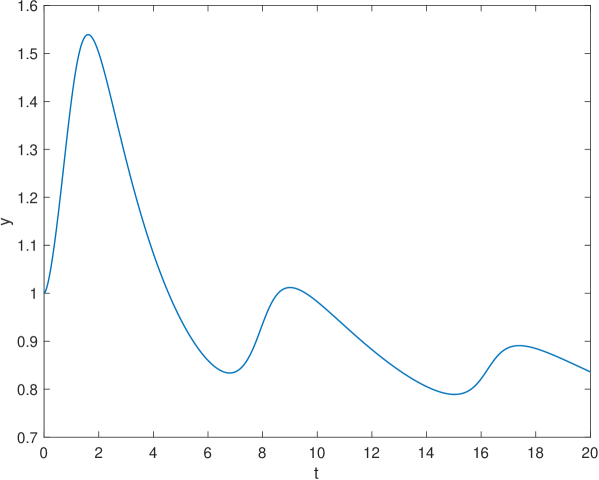
Figure 1: Reference solution for problem (49).

For solving problem (49), we use a uniform mesh with stepsize $h=20/400=1/20$. The method converges in 6 iterations, producing the following approximations:

$\ell$	$\rho_{\ell}$
0	.8360565285776644
1	1.115178544783084
2	1.057854760373079
3	1.006528883050734
4	.9999714859685488
5	.9999999991678453
6	.9999999999999855

Also in the case, it is possible to appreciate a quadratic-like convergence of the iteration. The maximum error in the final solution is $\approx 2\cdot 10^{-14}$, whereas the estimated one, by using is (44), is $6\cdot 10^{-14}$.

4.4 Example 4

We now consider the following linear FDE-TVP:

$$y^{(0.5)} = \left(\begin{array}[]{rr}-3&~{}0\\ -2&~{}-1\end{array}\right)y,\qquad t\in[0,2],$$

$$y(2) = \left(\begin{array}[]{c}2\,E_{0.5}\left(-3\cdot 2^{0.5}\right)\\[2.84526pt] E_{0.5}\left(-2^{0.5}\right)\end{array}\right)\simeq\left(\begin{array}[]{r}.2591172572977875\\[2.84526pt] .5953212597441289\end{array}\right),$$

having solution

$$y(t)=\left(\begin{array}[]{c}2\,E_{0.5}\left(-3\cdot t^{0.5}\right)\\[2.84526pt] E_{0.5}\left(-t^{0.5}\right)\end{array}\right),$$

corresponding to the initial value $y(0)=(2,\,3)^{\top}$. Since the vector field is linearly related to the solution, which has a singularity in the first derivative at the origin, we use a graded mesh with $h_{1}=10^{-14}$ and $N=100$. According to the result of Theorem 2.4, convergence is gained in just one iteration:

$\ell$	$\rho_{\ell}$
0	.2591172572977875	.5953212597441289
1	2.000000000000012	3.000000000000012

The maximum error in the final solution is $\approx 7\cdot 10^{-15}$, whereas the estimated one, by using (44), is $2\cdot 10^{-14}$.

4.5 Example 5

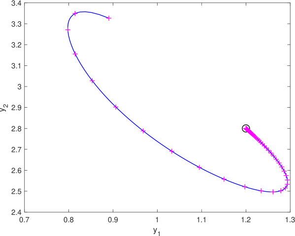
Figure 2: Reference solution for problem (52) (solid line). The circle denotes the actual initial condition, whereas the pluses denote the final approximate solution.

We now consider the following fractional Brusselator model:

$$y_{1}^{(0.7)} = 1-4y_{1}+y_{1}^{2}y_{2},$$ (52)

$$y_{2}^{(0.7)} = 3y_{1}-y_{1}^{2}y_{2},\qquad t\in[0,5],$$

$$y(5) = \left(\begin{array}[]{c}.8904632063462272\\[2.84526pt] 3.326603532694057\end{array}\right).$$ (55)

In such a case, the solution is not explicitly known, and we have computed the final value starting from $y(0)=(1.2,\,2.8)^{\top}$ by using the FHBVM(22,20) method with a graded mesh with $h_{1}=10^{-14}$ and $N=1000$: the reference solution is plotted in Figure 2 in solid line, with the initial condition marked by the circle. We solve the problem by using the FHBVM(22,20) method on a graded mesh with $h_{1}=10^{-14}$ and $N=200$. In so doing, the algorithm described in Table 1 converges in 5 iterations, with a quadratic-like order, obtaining the following results:

$\ell$	$\rho_{\ell}$
0	.8904632063462272	3.326603532694057
1	1.195221947994766	2.798766749634182
2	1.199608077826518	2.800213499824565
3	1.199998157974212	2.800001859877902
4	1.199999999973615	2.800000000034993
5	1.199999999999924	2.800000000000298

The maximum estimated error in the final solution is $\approx 10^{-13}$, whereas that in the final point is $\approx 4\cdot 10^{-16}$.

4.6 Example 6

As a last example, we consider a family of problems with $y\in\mathbb{R}^{2\nu}$ and

$$y^{(0.7)}=\left(\begin{array}[]{cc}&I_{\nu}\\ -I_{\nu}\end{array}\right)y+\cos(D_{\nu}y),\qquad t\in[0,5],$$ (56)

where $I_{\nu}\in\mathbb{R}^{\nu\times\nu}$ is the identity matrix, the function $\cos$ is meant to be applied in vector mode, and

$$D_{\nu}=\mathrm{diag}\left(1,\,2,\,\dots,2\nu\right)^{-1}.$$

The reference solution at $t=5$ has been computed by using the FHBVM(22,20) method on a graded mesh with $N=300$ and $n_{1}=10^{-14}$, solving (56) starting from the initial value with entries:

$$y_{i}(0)=\frac{1}{i}\cos\left((i-1)\frac{\pi}{\nu}\right),\qquad i=1,\dots,2\nu.$$ (57)

We solve the FDE-TVP (56) with $y(5)$ given, by using the FHBVM(22,20) method on a graded mesh with $N=35$ and $h_{1}=10^{-8}$, for $\nu=1,\dots,25$, thus solving FDE-TVPs having dimension 2, 4, …, 50.

The algorithm in Table 1 turns out to always converge in 5 iterations, except the problem of dimension 2 (i.e., for $\nu=1$), where convergence is obtained in 4 iterations. The error in the computed initial value is always less than $2\cdot 10^{-13}$. In Figure 3 is the plot of the execution mean times (over 5 runs) of the algorithm versus the dimension of the problem. In more detail, the figure plots:

• the total execution time (all times are in sec);

• the time for computing the required memory terms $\phi_{n-1}^{\alpha}(c,\rho_{\ell})$ (28) in the local problems (LPs);

• the time for solving the local problems (32) ;

• the time for computing the memory terms (37) in the local variational problems (LVPs);

• the time for solving the local variational problems (39).

According to Remark 3, we have not considered the pre-processing time for evaluating the integrals $I^{\alpha}P_{j}$ in (26) and $J_{j}^{\alpha}(x)$ (29), also because they require an extended precision arithmetic (quadruple precision would be enough) but, at the moment, they are computed symbolically in Matlab, and not numerically, so that this part of the code is not yet optimized.

From the obtained results, one may conclude that most of the computational time is spent in the solution of the variational problem: in particular, the evaluation of the memory terms for the local variational problems. Despite this, Algorithm 1, proves to be very effective, solving all problems with execution times ranging from approximately $10^{-1}$ sec to about 5 sec.

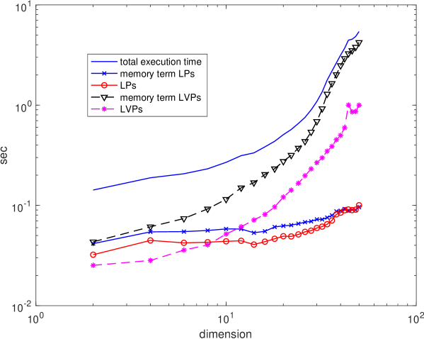
Figure 3: Execution times of Algorithm 1 for solving problem (56), with $y(5)$ given, for dimensions ranging from 2 to 50. See the text for details.

5 Conclusions

In this paper we have described a novel shooting procedure which, coupled with the Newton method, proves very appealing for numerically solving terminal value problems for fractional differential equations. The implementation details of the given procedure have been thoroughly given, when the underlying numerical methods are FHBVMs. These latter methods, when used as spectrally accurate methods in time, allow deriving very accurate solutions, along with a suitable estimate of the error in the computed solution. Numerical tests on both scalar and vector problems confirm the effectiveness of the approach.

Further directions of investigations include the extension for solving two-point boundary value problems, as well as the efficient numerical solution of the generated discrete problems. In particular, the solution of the local variational problems, due to the fact that they amount to solving just linear systems of algebraic equations.

Declarations.

The authors declare no conflict of interests, nor competing interests. No funding was received for conducting this study.

Data availability.

All data reported in the manuscript have been obtained by a Matlab^© implementation of the methods presented. They can be made available on request.

References

• (1) P. Amodio, L. Brugnano, F. Iavernaro. Spectrally accurate solutions of nonlinear fractional initial value problems. AIP Conf. Proc. 2116 (2019) 140005. https://doi.org/10.1063/1.5114132
• (2) P. Amodio, L. Brugnano, F. Iavernaro. Analysis of Spectral Hamiltonian Boundary Value Methods (SHBVMs) for the numerical solution of ODE problems. Numer. Algorithms 83 (2020) 1489–1508. https://doi.org/10.1007/s11075-019-00733-7
• (3) P. Amodio, L. Brugnano, F. Iavernaro. Arbitrarily high-order energy-conserving methods for Poisson problems. Numer. Algoritms 91 (2022) 861–894. https://doi.org/10.1007/s11075-022-01285-z
• (4) P. Amodio, L. Brugnano, F. Iavernaro. A note on a stable algorithm for computing the fractional integrals of orthogonal polynomials. Applied Mathematics Letters 134 (2022) 108338. https://doi.org/10.1016/j.aml.2022.108338
• (5) P. Amodio, L. Brugnano, F. Iavernaro. (Spectral) Chebyshev collocation methods for solving differential equations. Numer. Algoritms 93 (2023) 1613–1638. https://doi.org/10.1007/s11075-022-01482-w
• (6) L. Brugnano, K. Burrage, P. Burrage, F. Iavernaro. A spectrally accurate step-by-step method for the numerical solution of fractional differential equations. arXiv:2310.10526 [math.NA] https://doi.org/10.48550/arXiv.2310.10526 (submitted)
• (7) L. Brugnano, G. Frasca-Caccia, F. Iavernaro, V. Vespri. A new framework for polynomial approximation to differential equations. Adv. Comput. Math. 48 (2022) 76 https://doi.org/10.1007/s10444-022-09992-w
• (8) L. Brugnano, F. Iavernaro. Line Integral Methods for Conservative Problems. Chapman et Hall/CRC, Boca Raton, FL, USA, 2016.
• (9) L. Brugnano, F. Iavernaro. Line Integral Solution of Differential Problems. Axioms 7(2) (2018) 36. https://doi.org/10.3390/axioms7020036
• (10) L. Brugnano, F. Iavernaro. A general framework for solving differential equations. Ann. Univ. Ferrara Sez. VII Sci. Mat. 68 (2022) 243–258. https://doi.org/10.1007/s11565-022-00409-6
• (11) L. Brugnano, J.I. Montijano, F. Iavernaro, L. Randéz. Spectrally accurate space-time solution of Hamiltonian PDEs. Numer. Algorithms 81 (2019) 1183–1202. https://doi.org/10.1007/s11075-018-0586-z
• (12) L. Brugnano, J.I. Montijano, F. Iavernaro, L. Randéz. On the effectiveness of spectral methods for the numerical solution of multi-frequency highly-oscillatory Hamiltonian problems. Numer. Algorithms 81 (2019) 345–376. https://doi.org/10.1007/s11075-018-0552-9
• (13) K. Diethelm. The analysis of fractional differential equations. An application-oriented exposition using differential operators of Caputo type. Lecture Notes in Math., 2004. Springer-Verlag, Berlin, 2010.
• (14) K. Diethelm. Increasing the efficiency of shooting methods for terminal value problems of fractional order. J. Comput. Phys. 293 (2015) 135–141. https://doi.org/10.1016/j.jcp.2014.10.054
• (15) K. Diethelm, N.J. Ford, A.D. Freed. Detailed error analysis for a fractional Adams method. Numer. Algorithms 36 (2004) 31–52. https://doi.org/10.1023/B:NUMA.0000027736.85078.be
• (16) K. Diethelm, F. Uhlig. A new approach to shooting methods for terminal value problems of fractional differential equations. J. Sci. Comput. 97 (2023) 38. https://doi.org/10.1007/s10915-023-02361-9
• (17) N.J. Ford, M.L. Morgado. Fractional boundary value problems: analysis and numerical algorithms. Fract. Calc. Appl. Anal. 14 (2011) 554–567. https://doi.org/10.2478/s13540-011-0034-4
• (18) N.J. Ford, M.L. Morgado, M. Rebelo. High order numerical methods for fractional terminal value problems. Comput. Methods Appl. Math. 14 (2014) 55–70. https://doi.org/10.1515/cmam-2013-0022
• (19) R. Garrappa, Numerical evaluation of two and three parameter Mittag-Leffler functions. SIAM J. Numer. Anal. 53, No. 3 (2015) 1350–1369. https://doi.org/10.1137/140971191
• (20) R. Garrappa. Trapezoidal methods for fractional differential equations: Theoretical and computational aspects. Math. Comp. Simul. 110 (2015) 96–112. http://doi.org/10.1016/j.matcom.2013.09.012.
• (21) R. Garrappa. Numerical solution of fractional differential equations: a survey and a software tutorial. Mathematics 6(2) (2018) 16. http://doi.org/10.3390/math6020016
• (22) Z. Gu. Spectral collocation method for nonlinear Riemann-Liouville fractional terminal value problems. J. Compt. Appl. math. 398 (2021) 113640. https://doi.org/10.1016/j.cam.2021.113640
• (23) Z. Gu, Y. Kong. Spectral collocation method for Caputo fractional terminal value problems. Numer. Algorithms 88 (2021) 93–111. https://doi.org/10.1007/s11075-020-01031-3
• (24) C. Li, M.-M. Li, H. Zhou. Terminal value problem for a generalized fractional ordinary differential equation. Math. Meth. Appl. Sci. 44 (2021) 12963–12979. https://doi.org/10.1002/mma.7600
• (25) C. Li, Q. Yi, A. Chen. Finite difference methods with non-uniform meshes for nonlinear fractional differential equations. J. Comput. Phys. 316 (2016) 614–631. https://doi.org/10.1016/j.jcp.2016.04.039
• (26) Ch. Lubich. Fractional Linear Multistep Methods for Abel-Volterra Integral Equations of the Second Kind. Math. Comp. 45, No. 172 (1985) 463–469. https://doi.org/10.1090/S0025-5718-1985-0804935-7
• (27) I. Podlubny. Fractional differential equations. An introduction to fractional derivatives, fractional differential equations, to methods of their solution and some of their applications. Academic Press, Inc., San Diego, CA, 1999.
• (28) B. Shiri, G.-C. Wu, D. Baleanu. Terminal value problems for the nonlinear systems of fractional differential equations. Appl. Numer. Math. 170 (2021) 162–178. https://doi.org/10.1016/j.apnum.2021.06.015
• (29) M. Stynes, E. O’Riordan, J.L. Gracia. Error analysis of a finite difference method on graded meshes for a time-fractional diffusion equation. SIAM J. Numer. Anal. 55 (2017) 1057–1079. https://doi.org/10.1137/16M1082329
• (30) V. Lakshmikantham, D. Trigiante. Theory of Difference Equations: Numerical Methods and Applications. Academic Press Inc., Boston, 1988.