M³T: Multi-Scale Memory Matching for Video Object
Segmentation and Tracking

Abstract

Video Object Segmentation (VOS) has became increasingly important with availability of larger datasets and more complex and realistic settings, which involve long videos with global motion (e.g, in egocentric settings), depicting small objects undergoing both rigid and non-rigid (including state) deformations. While a number of recent approaches have been explored for this task, these data characteristics still present challenges. In this work we propose a novel, DETR-style encoder-decoder architecture, which focuses on systematically analyzing and addressing aforementioned challenges. Specifically, our model enables on-line inference with long videos in a windowed fashion, by breaking the video into clips and propagating context among them using time-coded memory. We illustrate that short clip length and longer memory with learned time-coding are important design choices for achieving state-of-the-art (SoTA) performance. Further, we propose multi-scale matching and decoding to ensure sensitivity and accuracy for small objects. Finally, we propose a novel training strategy that focuses learning on portions of the video where an object undergoes significant deformations – a form of “soft” hard-negative mining, implemented as loss-reweighting. Collectively, these technical contributions allow our model to achieve SoTA performance on two complex datasets – VISOR [10] and VOST [34]. A series of detailed ablations validate our design choices as well as provide insights into the importance of parameter choices and their impact on performance.

Abstract

This document provides additional material that is supplemental to our main submission. Section 6 describes the associated supplemental video. Section 7 includes additional implementation and dataset details, followed by Section 8 for additional experimental results and ablation studies. Finally, Section 9 details the societal impact of our work as standard practice in computer vision research.

Figure 1: Illustration of Our Approach. Given the first frame and the mask for the object of interest, our model adeptly tracks the object through the video via producing a sequence of segmentation masks. Despite potential transformations for the object, our approaches achieve decent performance in long videos (>20 sec) and videos with small object (<0.3% frame area). ${\dagger}$ denotes results reproduced by us using official code.

1 Introduction

Semi-automatic Video Object Segmentation (Semi-VOS) involves segmenting an object of interest in a video sequence given the provided initial mask in the first frame. This task has attracted significant attention in the literature [46] and is both interesting and challenging, involving aspects of detection/segmentation and temporal tracking.

Previous work on Semi-VOS often leverages memory matching, first proposed by Space-Time Memory networks (STM) [28]. The idea is simple, to encode the initial frame-mask pair (and, possibly later, frames and their inferred masks, as pairs) in neural memory, in order to perform spatiotemporal matching that helps mask prediction in new frame(s). A recent development focused on performing per-clip inference while utilizing this spatiotemporal memory matching instead of per-frame inference [29]. However, such approaches are challenged when objects are small (i.e., object size is small compared to patches used for matching) or when objects undergo significant deformations.

Recently, there has been rise in the Semi-VOS datasets dedicated to egocentric videos which focus on such complex deformations and long videos [34, 10]. In these datasets, objects can undergo extreme state changes, e.g., a banana being peeled/cut; or objects being molded into different shapes. Previous Semi-VOS approaches, especially memory-based ones, tend to face difficulty in such complex deformation scenarios [34]. Recent memory-based techniques that handled long videos [7, 16] or were able to associate multiple objects without adhoc post-processing [43] have shown relatively better performance. Nonetheless, current methods are not equipped with mechanisms specifically designed for these extreme state changes or small objects.

In this paper we focus on addressing the aforementioned challenges by proposing a novel DETR-style encoder-decoder framework for Semi-automatic Video Object Segmentation, featuring a clip-based windowed approach that excels in capturing objects in long videos, along with an incorporated multi-scale query-memory matching that enables adept handling of scenarios involving small and deforming objects. Illustration of our approach and improvements it achieves are shown in Fig. 1. The proposed multi-scale query-memory allows better local matching, which has significant impact on ability to deal with small objects or objects undergoing complex deformations. Further, the learned time-coding, within this memory, allows our model to leverage recency (nearby frames tend to be more relevant when segmenting a current one). Finally, based on an observation that abrupt state changes tend to deteriorate the performance, we propose a novel training strategy that focuses learning on portions of the video where object undergoes significant deformation. This can be thought of as a form of “soft” hard-negative mining, which, in practice, is implemented as loss-reweighting. Collectively, these design choices lead to SoTA performance on two challenging datasets – VISOR [10] and VOST [34].

Our contributions can be summarized as follows: (1) We propose a novel DETR-style encoder-decoder clip-based framework for Semi-VOS, capable of dealing with arbitrary long videos in windowed fashion. As part of this framework, we (2) introduce a novel multi-scale time-coded memory, designed to be particularly effective for objects that are small or can undergo complex deformations. We further, (3) introduce transformation-aware training objective that guides the model to focus learning on portions of the video where an object is transformed, thereby enhancing its ability to track objects across such changes. Finally, (4) through a series of detailed ablations we validate our design as well as provide insights into the importance of parameter choices (e.g., shorter clip and longer memory length) and their impact on performance. Experimental results demonstrate superior performance of our approach compared with previous state-of-the-art Semi-VOS techniques, resulting in $\approx 7\%$ improvement in VISOR [10] and $\approx 1\%$ in VOST [34] for all metrics. Especially, on longer videos and small objects of VOST, we outperform the next best method by $7\%$ and $2\%$, respectively.

2 Related Works

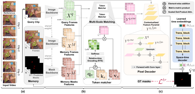
Figure 2: Overview of our approach. We divide an input video into non-overlapping clips of length $L$. For a query clip, we retrieve information on previous clips from our (a) Clip-based Memory in the form of frames and predicted (or initial reference) masks. We use a 2D-CNN backbone to obtain features for query frames $X^{q}$, and features for memory frames and masks, $X^{M}$ and $Y^{M}$ respectively. We then use our proposed (b) Multi-Scale Matching Encoder to perform dense matching at multiple-scales with frame features of the query clip $X^{q}$ and memory frames $X^{M}$, and use the resulting similarity between frames to obtain query clip’s mask features $Y^{q,enc}$ as a weighted combination of the memory mask features $Y^{M}$. In doing so, we modulate the similarity using our proposed Relative-Time Encoding (RTE) to learn recency of information in memory, thereby facilitating propagation over long-time spans. We then use (c) Multi-Scale Decoder to aggregate the resulting query clip’s mask features $Y^{q,enc}$ with clip’s frame features $X^{q}$ using Pixel Decoder to give contexualized feature pyramid $Y^{q,fpn}$. Finally, we use Space-Time Decoder to decode mask predictions $\hat{Y}^{q}$, by refining learned time embeddings on the contextualized feature pyramid $Y^{q,fpn}$. We update the memory with the predictions from last frame (=$L^{th}$ index) in the query clip, implemented as FIFO queue. During training, we use our transformation-aware loss $\mathcal{L}^{tr}$ to form segmentation loss for the entire video.

Video Object Segmentation (VOS). Video object segmentation separates foreground object(s) in a video from the background in a class agnostic manner. This task has two sub-categories [46]: automatic and semi-automatic. The former defines foreground object(s) based on their saliency in terms of appearance and motion, while the latter defines them based on manually initialized masks in the first frame of the video. In this work, we focus on semi-automatic formulation. Note, previously, this task was referred to as semi-supervised [30], which we avoid to reduce confusion with techniques that use additional unlabelled data [46].

Semi-automatic VOS (Semi-VOS). Semi-automatic methods perform segmentation and tracking with various challenges in terms of occlusions, objects deformation, motion blur, tracking of small objects and differentiating similar ones. Recently, there are some benchmarks proposed on egocentric videos [10, 34, 45] with few focusing on objects undergoing extreme state changes, e.g., eggs being broken. Tracking objects under these extreme changes, where shape, consistency, colour and texture of the object drastically change, presents additional challenges.

Semi-VOS approaches can be categorized into online fine-tuning based [38, 41, 36, 4], propagation based [20, 19, 3] and matching based [17, 37, 28, 43] methods. Matching based methods, usually relying on memory-based techniques, have proven to be most effective and robust [28, 43, 29, 7]. We build on this line of works, but propose an approach that is specifically designed to accommodate the aforementioned challenges in egocentric videos.

Role of memory in VOS. Space-Time Memory (STM) [28] proposed a memory-based technique that spawned multiple consequent approaches [43, 7, 29, 16]. AOT [43] extended memory reading to track multiple objects simultaneously, while incorporating both global and local attention mechanisms. XMem [7] extended the use of memory for long-video sequences by creating memory modules at three different time-levels: long-term, short-term and per-frame. While previous methods focused on per-frame inference, PCVOS [29] proposed inference and updates to memory on a clip-level. Overall, these methods focused on matching with the memory bank on a single-spatial scale. However, in this work, we propose multi-scale memory matching and decoding which is particularly effective for small objects. Similar to PCVOS [29], we use clip-based memory updates, but in addition we propose a relative time-encoding for memory to learn recency, particularly useful for long-videos. Compared to XMem [7], our time-encoding is learned on per-frame level instead of three explicit time-levels. Finally, unlike previous works we propose a transformation-aware loss that takes state changes into account as a form of hard-negative mining during train.

3 Approach

Given a video, a reference frame and the corresponding ground-truth segmentation mask indicating the object of interest, our goal is to predict the sequence of segmentation masks of the object for all the frames in the video.

3.1 Overview

Our model builds on DETR-style video encoder-decoder architectures [5, 40, 6]. Our motivation is to track objects through challenging scenarios (e.g., tracking small objects) and under extreme state changes across long videos. Therefore we endow the aforementioned architecture with three key components; (i) multi-scale matching encoder, (ii) clip-based memory, and (iii) multi-scale decoder.

Given an input video and ground-truth segmentation mask of a desired object, we make predictions by sub-dividing the video into non-overlapping clips, and processing the resulting clips in a sequential order while propagating information through the use of the clip-based memory.

Fig. 2 shows an overview of our approach. For each query clip, we encode frames in the clip using a 2D-CNN visual backbone, yielding frame-features (or tokens) at multiple-scales or feature hierarchies. Mask predictions of previous video clips or ground-truth, for the first frame, are taken as memory. We perform dense token matching between frame features of the query clip and memory at multiple-scales using our Multi-Scale Matching Encoder to obtain similarity between the query and past clips. In particular, we use Relative Time Encoding (RTE) for memory to encode relative time difference of past clips w.r.t. the current query clip. Thus, our approach enables more accurate long temporal context modelling. We use the resulting similarity to obtain encoded mask features for the query clip as a weighted combination of the memory mask features. Such multi-scale matching enables propagating object mask from memory, which is especially useful to track small objects. We then obtain feature-pyramid for decoding by incorporating the query clip frame-features with encoded mask features in a multi-scale fashion. Finally, we use Space-Time Decoder [40] to decode mask predictions from feature pyramid for the query clip. We then update the memory with the query clip frame features and mask predictions to be used for the next clip. During training, we use Transformation-aware Reweighting to re-weigh clip segmentation loss [5] over time. This can be interperted as a form of “soft” hard-negative mining, to account for object transformations which are tightly coupled to the change in relative area, position and number of connected parts of the ground-truth object. We discuss details of our proposed modules in the following sections.

3.2 Multi-scale Matching Encoder

For a query video clip of length $L$, we encode each frame independently using a ResNet [14] to obtain frame features $X^{q}=\{\mathbf{x}^{q}_{s}\}_{s\leq S}$, where $\mathbf{x}^{q}_{s}\in\mathbb{R}^{L\times h_{s}\times w_{s}\times d_{s}}$ is the feature map of query clip at scale $s$. The total number of scales are denoted by $S$, and $h_{s}$, $w_{s}$ and $d_{s}$ are height, width and channels of the feature map at scale $s$.

Inspired by previous work [21], originally designed for few-shot tasks and operating on single images, we propose a multi-scale query-memory matching module for dense prediction tasks. We compute similarity between frame features of query and memory at multiple-scales, and obtain mask features for the query clip as a weighted combination of the memory mask features. We define a memory with a maximum size of $N$, and the elements stored in the memory are denoted as $\{X^{M},Y^{M}\}$ , where $X^{M}=\{\mathbf{x}^{m}_{s}\}_{s\leq S}$, $Y^{M}_{i}=\{\mathbf{y}^{m}_{s}\}_{s\leq S}$ are frame and mask features respectively in memory, s.t. $\mathbf{x}^{m}_{s},\mathbf{y}^{m}_{s}\in\mathbb{R}^{n\times h_{s}\times w_{s}\times d_{s}}$, with a total size of $n$ ($n\leq N$). The memory contains features of past video clip frames and predicted masks (along with the reference ground-truth frame). We describe update operations applied to memory in Sec. 3.4.

For each scale $s$, we use multi-head attention layer (MHA) for token matching [35, 21], where we get tokens for query frames $\{\mathbf{q}_{s}\}_{s\leq S}$ and memory $\{\mathbf{k}_{s},\mathbf{v}_{s}\}_{s\leq S}$ by applying linear projection and adding 2D positional encoding to query frame features $X^{q}$, and memory frame and mask features $\{X^{M},Y^{M}\}$ respectively, where $\mathbf{q}_{s}\in\mathbb{R}^{Lh_{s}w_{s}\times d}$ and $\mathbf{k}_{s},\mathbf{v}_{s}\in\mathbb{R}^{nh_{s}w_{s}\times d}$ after flattening the tokens, and $d$ is hidden dimension. The query clip’s encoded mask tokens are obtained for each scale $s$ using,

$$\mathbf{y}^{q,enc}_{s}=\text{MHA}(\mathbf{q}_{s},\mathbf{k}_{s},\mathbf{v}_{s})=\left[\mathbf{o}_{1},...,\mathbf{o}_{H}\right]w_{s}^{O},$$ (1)

$$\mathbf{o}_{h}={\tt Softmax}\left(\frac{\mathbf{q}_{s}w_{h,s}^{Q}(\mathbf{k}_{s}w_{h,s}^{K})^{T}}{\sqrt{d_{H}}}\right)\mathbf{v}_{s}w_{h,s}^{V},$$ (2)

where $H$ is number of heads, $d_{H}$ is the channels, $w^{Q}_{h,s},w^{K}_{h,s},w^{V}_{h,s}\in\mathbb{R}^{d\times d_{H}}$ and $w_{s}^{O}\in\mathbb{R}^{Hd_{H}\times d}$ for scale $s$ and $\left[.\right]$ is the concatenation operator. After reshaping the encoded mask tokens, we obtain the query clip’s encoded mask features denoted as $Y^{q,enc}=\{\mathbf{y}^{q,enc}_{s}\}_{s\leq S}$, where $\mathbf{y}^{q,enc}_{s}\in\mathbb{R}^{L\times h_{s}\times w_{s}\times d}$.

Relative Time Encoding (RTE). As described above, the token matching in previous work [21] is designed for static image object segmentation tasks. However, in our setting of video object segmentation, images stored in the memory form a sequence of frames from the given video, and the visual appearance of the foreground object may change significantly, especially in videos with object transformations. To address this issue, we propose Relative-Time Encoding (RTE) for our matching encoder to learn the importance of each frame in the memory when conducting token matching, thereby reducing the potential drift in matching on frames in the memory far from the current timestep.

Specifically, RTE makes the matching dependent on time by modulating similarity weights in Eq. 2 and helps learn associations based on recency, which is especially useful for extending memory over long-time spans. In particular, based on the memory bank size (=$N$), we define a learnable embedding set as $\{e_{i}\in\mathbb{R}^{1\times i}\}_{i=1}^{N}$. Depending on the number of elements $n$ in the memory, we select the corresponding $e_{n}$ to modulate the similarity weights. Specifically, we first expand $e_{n}\in\mathbb{R}^{1\times n}$ to $E_{n}\in\mathbb{R}^{Lh_{s}w_{s}\times nh_{s}w_{s}}$ by broadcasting the values along the 1-dim and reshaping. And then, we incorporate RTE into Eq. 2 as follows,

$$\mathbf{o}_{h}={\tt Softmax}\left(E_{n}\circ\frac{\mathbf{q}_{s}w_{h,s}^{Q}(\mathbf{k}_{s}w_{h,s}^{K})^{T}}{\sqrt{d_{H}}}\right)\mathbf{v}_{s}w_{h,s}^{V},$$ (3)

where $\circ$ represent element-wise multiplication. Please refer to Experiments (Sec. 4.4) for more details.

3.3 Multi-scale Decoder

We obtain feature pyramid (see [6]) by contexualizing query frame features with the encoded mask features. The motivation is that the use of such high-resolution feature pyramid during decoding would lead to better performance for small objects. And finally, we make use of Space-Time Decoder [40] to decode mask predictions from the contextualized feature pyramid for the query clip.

Contexualized feature pyramid. We obtain feature pyramid for the query clip’s mask features $Y^{q,fpn}$ by aggregating query clip’s image features $X^{q}$ with the encoded multi-scale mask features $Y^{q,enc}$. Specifically, for each scale $s$ in 32, 16, and 8 output stride, we add $\mathbf{y}^{q,enc}_{s}$ to contextualize the feature pyramid with the encoded mask features for query clip, as shown in Fig. 2 (c).

$$\tilde{\mathbf{y}}^{q,fpn}_{s}={\tt Conv2D}(\mathbf{x}^{q}_{s})+{\tt Upsample}(\mathbf{y}^{q,fpn}_{s-1})+\mathbf{y}^{q,enc}_{s}$$ (4)

$$\mathbf{y}^{q,fpn}_{s}={\tt Conv2D}\left(\tilde{\mathbf{y}}^{q,fpn}_{s}\right),$$ (5)

where Conv2D and Upsample operations are applied frame-wise. Different from conventional FPN [24, 6], we aggregate frame features with the encoded mask features (last term in Eq. 4) to obtain feature pyramid $Y^{q,fpn}=\{\mathbf{y}^{q,fpn}_{s}\}_{s\leq S}$, where $\mathbf{y}^{q,fpn}_{s}\in\mathbb{R}^{L\times h_{s}\times w_{s}\times d}$.

Space-Time Decoder.

We use learned time embeddings $\{\mathbf{t}_{j}\}_{j\leq L}\in\mathbb{R}^{d}$, equal to the length of query clip, and refine them over multiple decoder blocks using the encoded contextualized features $Y^{q,fpn}$ to obtain final mask predictions. In particular, within each decoder block, space-time attention is factorized over time and space by performing temporal self-attention and spatial frame-wise cross-attention operations, interleaved with feed-forward and normalization layers [40]. First, the temporal self-attention allows time embeddings to attend to each other, thereby facilitating temporal interactions across the video clip. Second, the frame-wise cross-attention performs cross-attention with each frame separately, where for a $j^{th}$ frame, the corresponding time embedding $\mathbf{t}_{j}$ cross-attends to its encoded contextualized features $\mathbf{y}^{q,fpn}_{j,s}\in\mathbb{R}^{h_{s}\times w_{s}\times d}$. By stacking multiple decoder blocks, the time embeddings gets refined in a hierarchical manner to give $\{\mathbf{\hat{t}}_{j}\}_{j\leq L}$, and the final mask prediction is obtained by taking dot-product of $\{\mathbf{\hat{t}}_{j}\}_{j\leq L}\in\mathbb{R}^{d}$ with the highest scale (=$S^{th}$) contextualized feature $\{\mathbf{y}^{q,fpn}_{j,S}\}_{j\leq L}\in\mathbb{R}^{h\times w\times d}$ frame-wise to yield $\hat{Y}^{q}=\{\mathbf{\hat{y}}^{q}_{j}\}_{j\leq L}\in[0,1]^{h\times w}$, as per-pixel probabilities.

The stacking of multi-scale decoding blocks and the use of multi-scale contextualized features is similar to Mask2Former [6]. Specifically, we use $6$ decoder blocks, where each block receives contextualized features starting from lowest scale $s$ in a round-robin fashion with the appropriate addition of positional encoding and scale-embedding.

Unlike PCVOS [29], which performs encoding for each frame in query clip independently and performs intra-clip refinement through dense transformer-based attention, we make use of temporal self-attention of time-embeddings to share information within clips in order to account for intra-clip refinement.

3.4 Clip-based Memory Module

We divide the input video into non-overlapping clips of length $L$, and process the video and update memory sequentially one clip at a time. The intuition being that clip-level updates to memory, compared to updates at every frame, trades-off performance with compute time and GPU memory, and at the same time enables long-range modelling [29]. In particular, we perform an update to memory $\{X^{M},Y^{M}\}$ by appending features for frame and predicted mask of the last frame in the query clip (=$L^{th}$ index), i.e., $\{X^{q}_{L},\hat{Y}^{q}_{L}\}$. The memory is implemented as a FIFO (first-in-first-out) queue, which initially gets populated with the features of frame and ground-truth mask of the initial reference frame. We keep the reference frame fixed in memory (as the first index in memory), to have a notion of the initial state of the object if in case there is too much divergence [16]. Lastly, we use the same visual backbone used for frames to encode masks as well.

3.5 Transformation-aware Reweighting

In our case, objects within a video may undergo transformations, leading to significant changes in their visual appearance and shape. However, treating frames uniformly when forming video-level loss, as done in previous VOS works [43, 29] could lead to sub-optimal solutions. The reason being that majority of frames contributing to learning are relatively simple, causing redundancy over long-time spans, resulting in failure to track objects of interest post complex transformations.

To address this issue, we frame our objective as an unbalanced learning problem, where the object transformation only occupies a small part of the entire video. We design a reweighting factor to enable the model to place greater emphasis on objects during transformations. Specifically, we define our transformation-aware video-level loss as $\mathcal{L}^{\text{tr}}_{\text{total}}=\alpha_{1}\mathcal{L}_{\text{dice}}+\alpha_{2}\mathcal{L}^{\text{tr}}_{\text{focal}}$, where $\mathcal{L}_{\text{dice}}$ is image-based DICE/F-1 loss [27], and $\mathcal{L}^{\text{tr}}_{\text{focal}}=\frac{1}{L}\sum^{L}_{t=1}w^{t}\times l^{t}_{focal}$, where $l^{t}_{focal}$ is the focal loss [25] for $t$-th frame, and $w^{t}$ denotes weight assigned to $t^{th}$ frame. $\alpha_{1}$ and $\alpha_{2}$ are hyperparameters to modulate relative importance of loss terms. Overall, we aim to assign higher weights to frames where the object of interest undergoes transformation. In our fully-supervised setting, we generate weights using ground-truth segmentation masks for the frames in a video, denoted as $M_{1},M_{2},\dots,M_{L}$. Empirically, we found that simply computing the change in area of consecutive ground truth masks is a good indicator to identify frames containing complex transformations. Our observation is that during transformation phase, the object gets split/cut, molded, sheared into a different state, resulting in noticeable change in the area of the mask. Based on this, we formulate the weights $\{w^{t}\}_{t\leq L}$ as,

$$w^{t}=\frac{e^{\delta^{t}/\tau}}{\sum^{L}_{t=1}e^{\delta^{t}/\tau}}\times L\text{, where }$$ (6)

$$\delta^{t}=\frac{\|\mathcal{A}(M^{t})-\mathcal{A}(M^{t-1})\|}{\sum^{L}_{t=1}\|\mathcal{A}(M^{t})-\mathcal{A}(M^{t-1})\|/L}.$$ (7)

We note that $\mathcal{A}(M)$ represents the foreground area of the given mask $M$, and $\tau$ is a temperature parameter for the Softmax operation. Note that we also explore alternate methods to compute $\delta^{t}$ as a function of change in the number of connected components and change in the center of mass of object of interest. Please find details in the Suppl. materials.

4 Experiments

We empirically show our method’s ability to achieve high-quality video object segmentation and tracking with long-term pixel-level consistency during object transformations. Our approach outperforms existing state-of-the-art methods on VISOR [10] and VOST [34] benchmarks. Lastly, we conduct extensive analyses to validate our design choices.

Approach	Pre-train Static	Fine-Tune VISOR	$\mathcal{J}\&\mathcal{F}$	$\mathcal{J}$	$\mathcal{F}$	$\mathcal{J}\&\mathcal{F}_{\text{unseen}}$
STM [28, 10]	✓		56.9	55.5	58.2	48.1
STM [28, 10]	✓	✓	75.8	73.6	78.0	71.2
M3T (Ours)	✓		63.7	61.5	65.9	56.3
M3T (Ours)	✓	✓	82.9	80.6	85.1	81.5

Table 1: Val performance on VISOR. Under similar pre-training and backbone configurations, our method outperforms best reported results, with a marginal drop in unseen performance (=$1.4\%$) compared to STM [28, 10] (=$4.6\%$). Performance numbers on STM [28] are reported from VISOR [10].

4.1 Implementation Details

We follow a two-stage training protocol similar to prior works [46, 28, 43, 22], where we first pre-train our model using synthetic video sequences generated from static image datasets [8, 12, 13, 33, 23], and then fine-tune on target benchmarks. Consistent with prior works, we use ResNet-50 [14] as the backbone for image encoder and mask encoder with shared weights. In our Multi-Scale Matching Encoder, if not specified, we use feature maps from last two layers of the visual backbone at strides $32$ and $16$. During training, we use video length of 12, with clip length $L=2$, and a memory bank size of $N=7$. We use AdamW [26] optimizer with $2e^{-5}$ learning rate over 20 epochs with $624$ and $480$ image resolution for VOST and VISOR respectively. For the clip-based memory, we retain the ground truth for the initial reference frame and mask as the first element. We perform updates by storing the last frame and its predicted mask features for each clip in the memory in a FIFO fashion. During inference, we process the entire video clip-by-clip to predict the results. Details in Suppl.

4.2 Datasets and Evaluation

We evaluate on two benchmark datasets consisting of egocentric videos with pixel-level mask annotations. (1) VISOR [10] contains $7,836$ videos, sourced from Epic-Kitchens [9] dataset, with an average video length of $12.0$ seconds or $6$ frames per video at $0.5$ FPS, and (2) VOST [34] is a recently proposed dataset designed for video object segmentation under complex transformations. The videos in VOST have longer duration and more complex transformations compared to VISOR. VOST contains $713$ videos with an average length of $21.2$ seconds or $106$ frames per video at $5$ FPS. More details are in the Suppl.

To evaluate quality of our predicted masks, we use metrics commonly used in Video Object Segmentation, i.e., a combination of region similarity ($\mathcal{J}$) and contour accuracy ($\mathcal{F}$) [34, 10, 30, 39, 31]. We note that, VOST [34] introduced an additional metric, $J_{tr}$, designed to evaluate predictions occurring after object transformations. Unlike the standard $J$, $J_{tr}$ evaluates on last $25\%$ of frames in a video sequence, capturing performance of object transformations occurring later in videos. Moreover, following VISOR [10], we additionally report results on both seen and unseen subsets of the validation set to assess model’s generalization.

4.3 Main Results

Approach	Pre-training	VOST
		$\mathcal{J}_{\text{tr}}$	$\mathcal{J}$
OSMN-Match [41]	Static + DAVIS [31]	7.0	8.7
OSMN-Tune [41]	Static + DAVIS	17.6	23.0
CRW [18]	ImageNet [11] + DAVIS	13.9	23.7
HODOR-Img [1]	COCO [23] + DAVIS	13.9	26.2
HODOR-Vid [1]	COCO + DAVIS	25.4	37.1
CFBI [42]	ImageNet + COCO + DAVIS	32.0	45.0
CFBI+ [44]	Static + DAVIS	32.6	46.0
XMem [7]	Static + DAVIS	33.8	44.1
AOT† [43]	Static	35.1	47.1
AOT [43]	Static + DAVIS	36.4	48.7
M3T (Ours)	Static	36.5	48.2
M3T (Ours)	Static + DAVIS	37.7	49.3

Table 2: Val performance on VOST. Our method outperforms the best reported results on both $\mathcal{J}$ and $\mathcal{J}_{\text{tr}}$ metrics. We note that Static represents a collection of image datasets [8, 12, 13, 33, 23]. Performance numbers on the above prior works are reported from VOST [34]. ^† denotes results reproduced by us using official code.

	OSMN Tune [41]	CFBI+ [44]	HODOR Vid [1]	AOT [43]	M3T (Ours) (diff with AOT [43])
All	17.6	32.6	25.4	36.4	37.7 (+1.3)
LNG	12.4	30.4	25.0	34.7	41.9 (+7.2)
MI	14.7	26.4	20.6	27.2	29.2 (+2.0)
SM	14.4	23.3	16.6	24.7	26.6 (+1.9)

Table 3: Quantitative analysis of various factors in VOST val set. We report $\mathcal{J}_{\text{tr}}$ score for each case. LNG: the subset comprising long videos, MI: the subset with multi-instances and SM: the subset with small objects. We report the gain, (.), w.r.t the best reported model, AOT [43]. ^† denotes results reproduced by us using official code.

Comparison to prior works.

Table 1 shows comparison on VISOR. Our model outperforms the previous best model STM [28] by $7.1\%$ on $\mathcal{J}\&\mathcal{F}$ and $10.3\%$ on $\mathcal{J}\&\mathcal{F}_{\text{unseen}}$. We note that, in unseen setting, STM [28] reports a considerable $4.6\%$ ($75.8\rightarrow$ 71.2) drop in $\mathcal{J}\&\mathcal{F}_{\text{unseen}}$, whereas our method only shows $1.4\%$ ($82.9\rightarrow$ 81.5) drop. This suggests stronger generalization ability of our proposed approach and its robustness in new environments.

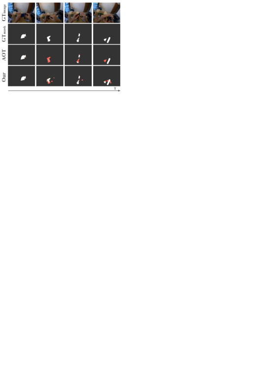
Figure 3: Qualitative comparison on VOST. Best viewed in color; red indicates incorrect predictions. Our method is able to track and delineate the object’s boundary with fine details under complex deformation, e.g. cutting onions, compared to best prior work, AOT [43].

To further validate our ability to track objects in long-videos with complex object transformations, we report results on VOST dataset in Table 2. Our model outperforms the previous best model, AOT [43], both in terms of $\mathcal{J}$ and $\mathcal{J}_{\text{tr}}$ under the same pre-training and backbone configuration. Notably, our model achieves comparable performance without relying on the additional DAVIS [31] dataset in the pre-training phase.

Furthermore, in order to quantitatively investigate various factors affecting the performance, e.g., video length (LNG) (>20 sec), the presence of multiple instances (MI), and small objects (SM) (<0.3% frame area), we follow the evaluation protocol outlined in VOST [34] by evaluating on subsets of validation data representing the above mentioned factors. The comparison is shown in Table 3. Our method achieves best scores compared to all previous methods, reported in VOST [34], in terms of the three factors (i.e., LNG, MI, and SM), confirming the tracking capability of our model in challenging scenarios. Specifically, we show the highest gain w.r.t. AOT [43], in the long video (LNG) case ($+7.2\%$) due to our multi-scale query-memory matching and decoding framework.

Qualitative results. We compare our proposed method with the prior best model, AOT [43], on VOST. Qualitative examples are shown in Fig. 3. We select an example from the validation set, present in both the long video and multi-instance subset. We observe that AOT’s outputs struggle to maintain long-term consistency for the same object across the long sequence, resulting in confusion between different parts of multiple “onions” while cutting one. In contrast, our method, which incorporates a clip-based memory module and the multi-scale matching and decoding strategy, effectively preserves consistency across long sequences for the objects. This enables us to generate accurate masks for each object without mixing them. For video version of this example and additional qualitative results, please refer to our supplementary materials.

#	Video	$L$	Memory		$\mathcal{L}^{\text{tr}}_{\text{focal}}$	Scales	$\mathcal{J}_{\text{tr}}$	$\mathcal{J}$
	length		$N$	RTE
w/ different video lengths
(1)	9	2	3	$\checkmark$		2	30.7	44.5
(2)	12	2	3	$\checkmark$		2	32.9	45.4
(3)	12	2	7	$\checkmark$		2	33.7	47.2
(4)	15	2	7	$\checkmark$		2	32.6	47.0
w/ different memory bank sizes, $N$
(5)	12	2	1	$\checkmark$		2	27.4	40.5
(6)	12	2	3	$\checkmark$		2	32.9	45.4
(7)	12	2	5	$\checkmark$		2	32.0	45.8
(8)	12	2	7	$\checkmark$		2	33.7	47.2
w/ different clip lengths, $L$
(9)	12	1	7	$\checkmark$		2	32.3	47.1
(10)	12	2	7	$\checkmark$		2	33.7	47.2
(11)	12	2	5	$\checkmark$		2	32.0	45.8
(12)	12	3	5	$\checkmark$		2	34.9	46.5
w/ or w/o RTE
(13)	12	2	7			2	31.4	45.3
(14)	12	2	7	$\checkmark$		2	33.7	47.2
Number of scales used in multiscale matching
(15)	12	2	7			1	22.5	33.9
(16)	12	2	7			2	31.4	45.3
(17)	6	2	4			3	27.2	40.2
w/ or w/o Transformation-aware Loss $\mathcal{L}^{\text{tr}}_{\text{focal}}$
(18)	12	2	7			2	32.3	45.6
(19)	12	2	7		$\checkmark$	2	33.5	46.6
(20)	12	2	7	$\checkmark$	$\checkmark$	2	36.5	48.2

Table 4: Ablation study on VOST val set. We examine various parameter combinations, where BS represents the bank size of the memory, and RTE denotes relative time encoding. Note that numbers with $\underline{\text{underline}}$ represents best performance within ablation group, and bold the overall best.

4.4 Ablation Study and Model Analysis

To verify the effectiveness of key design elements in our model, we conduct ablation studies and model analysis with different settings on VOST [34]. The results are shown in Table 4. We consider six different cases,

Video length. We examine the impact of video length used during training. Rows (1-4) show that a video length of $12$ achieves the best performance when compared to shorter (i.e., $9$) and longer (i.e., $15$) video lengths.

Bank size ($N$). Rows (5-8) indicate that increase in the memory bank size results in better performance. However, this expansion requires extending the video length to store more frames in memory, demanding additional computational resources. GPU memory limitations cap our memory bank size at $7$. We believe that training on GPUs that can accommodate larger memory bank, could lead to further improvements.

Clip length ($L$). Rows (9-12) show that clip-level inference and memory updates perform better than frame-level ($L=1$). In addition, PCVOS [29] found that using even longer clip lengths ($>10$) results in decrease in performance. In our case, building on the above trade-off on clip length, and taking into account our design choices (multi-scale matching and decoding) together with limitations on GPU memory, we use clip length of $2$ for our final model.

Relative-time encoding (RTE). Rows (13-14) show that our proposed time-coded memory improves the results. We visualize the learned embeddings ($e_{n}\in\mathbb{R}^{1\times n}$) of our RTE in Fig. 4 in the case of $n=\{4,5,6\}$, where $n$ is the number of frames in memory. The results indicate that our RTE equips the model with the flexibility to determine the importance of each frame in memory during the matching process. Notably, we observe that during matching, a query frame relies more on the two closest frames (indices $0$ and $1$) compared to those farther away. Moreover, regardless of the number of frames in the memory, the first frame always holds significance as it represents the ground truth / reference mask. For the complete version of these qualitative results, please see Suppl.

Multi-scale matching encoder. Rows (15-17) show that using single-scale (=$1$) results in significantly lower performance, confirming the need for our multi-scale matching and decoding. Training on three-scales (row 17) faces GPU memory limitations which requires lowering video length and memory bank size, leading to lower performance compared to two-scales (row 16). We also qualitatively explore the effectiveness of this multi-scale design in Fig. 5. We select a video featuring small objects, and plot attention heat maps produced by our multi-scale matching encoder. We observe that our model is able to finely match small objects in feature maps at multiple-scales. In particular, in the third column (or frame), we observe that the attention at the coarse-scale (=$1$) is scattered on human hand and other parts of the frame, however on finer-scale (=$2$), it successfully attends to the object of interest. These findings illustrate the ability of our multi-scale matching to capture small objects. We provide additional results in the Suppl.

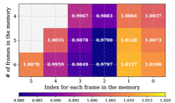
Figure 4: Visualization of RTE. Value in each grid represents the learned importance score for each frame w.r.t. different number of frames in the memory ($n$). Lighter colors indicate higher scores.

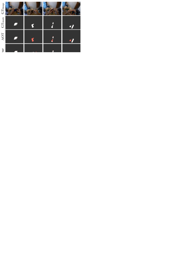
Figure 5: Visualization of the attention maps in the multi-scale matching modules. Scale 1 has a resolution of $\frac{1}{32}$ of the input frame, and scale 2 is at $\frac{1}{16}$ resolution. Best viewed in color; lighter colors indicate higher attention scores. The red box in the first frame denotes the object of interest in the query frame.

Transformation-aware reweighting. Rows (18-20) confirm the efficacy of our proposed loss which incorporates a “soft” hard negative-mining on video-level loss during training. Based on the above observations, we choose the final model configuration for optimal performance during training: a video length of $12$ frames, a clip length of $2$, a memory bank size of $7$, with RTE, with multi-scale matching using $2$ scales and with transformation-aware loss.

We provide further ablations on the relative-time encoding and transformation-aware loss in the Suppl. materials.

5 Conclusion

In this paper, we proposed a novel multi-scale memory matching and decoding scheme with clip-based time-coded memory for Semi-VOS task, designed to cope with complex object transformations, small objects and long video tracking. Moreover, we proposed a technique for hard negative mining through a novel transformation-aware loss. Our results show that the proposed model outperforms previous state-of-the-art on Semi-VOS across two benchmarks, with significant gains on VISOR benchmark up to 10%.

Supplementary Material

6 Supplemental Video

We include an accompanying supplemental video - video_demo.mp4 - as part of the supplemental materials. In this video we show qualitative segmentation results of our approach on the two benchmarks VOST [34] and VISOR [10]. For VOST, we show predictions on three videos showing our method’s capability on small and multiple instances of objects compared to the previous best state-of-the-art method, AOT [43]. We additionally include a failure case as well. For VISOR, we show three videos showing our method’s tracking capability over the previous best method, STM [28], including a failure case as well. The video is in MP4 format and $3$ minutes $10$ seconds long. The codec used for the realization of the provided video is H.264 (x264).

7 Implementation and dataset details

Training.

During training, we use AdamW [26] optimizer with weight decay $1e^{-4}$, learning rate $1e^{-5}$ for the backbone and $2e^{-4}$ for the rest of the model. We train for 20 epochs and reduce learning rate by $1/10^{th}$ factor at the $8^{th}$ and $16^{th}$ epoch. Similar to AOT [43], we use random resizing and cropping for data augmentation, avoiding additional augmentations to ensure a fair comparison. We uniformly use batch size of $1$ per GPU, and conduct experiments on VOST and VISOR datasets using $4$ Nvidia A40 and $8$ Nvidia T4 GPUs respectively. We use video lengths of $12$ and $6$ for VOST and VISOR respectively, necessitating the use of higher GPU memory in the case of VOST compared to VISOR. The input image resolution is set to $480$ and $624$ pixels on shorter side (keeping the aspect ratio same) on VISOR and VOST respectively.

Architecture.

Our model is built on ResNet-50 [14] backbone, which excludes dilation in the last convolutional block compared to STM and related approaches [28, 29]. The backbone is shared for encoding both the images and masks. Keeping in line with TubeDETR [40], we use fixed-sinusoidal 2D positional embedding for both image and mask features. For multi-scale query matching, we use a multi-head attention layer [21] with a hidden size of $256$ and $4$ heads for each scale. We perform LayerNorm [2] on queries and keys before multi-head attention, and on output after the multi-head attention. We use GELU [15] activation function on the residual connection for the output, and use a $10\%$ attention dropout to reduce overfitting.

Our decoder consists of a pixel decoder [6] and a space-time transformer decoder [40] used after the multi-scale matching encoder. The pixel decoder [6] produces feature-pyramid at four scales using a combination of lateral and output Conv layers, with the hidden dimension / output channel size of $256$. And the space-time transformer decoder [40] incorporates $6$ layers of multi-head attention, comprising $8$ heads with a hidden dimension of $256$. For the output, we use ReLU as the activation function and maintain a $10\%$ dropout rate during training.

Dataset	Videos (train/val)	Frames (train/val)	Avg. len. (sec)	Ann. fps	Avg. obj size (% of frame)
VISOR	5.3k / 1.2k	33k / 7.7k	12.0	0.5	6.67
VOST	572 / 70	60k / 8k	21.2	5.0	2.57

Table 5: Dataset statistics for VISOR and VOST. Avg. len. stands for average video length, and Ann. fps denotes annotation frames per second.

Dataset.

The data statistics for VOST [34] and VISOR [10] are outlined in Tab. 5. Notably, the videos in VOST are twice as long in duration compared to VISOR. In particular, for VOST, the average length of videos is $21.2$ seconds, annotated at $5$ frames-per-second (fps). This amounts to approximately $106$ annotated frames per video on average. In comparison, VISOR includes $6$ annotated frames per video with a much lower $0.5$ annotation frame rate (fps).

Both datasets focus on egocentric videos, thereby resulting in relatively smaller average object sizes in comparison to the conventional video object segmentation datasets [31]. Specifically, VOST’s average object size equates to $2.57\%$ of the frame size, whereas VISOR’s average object size corresponds to $6.67\%$ of the frames. This indicates that designing a model tailored for objects of various sizes (including small objects) is essential in egocentric videos, which is tied to various applications in robotics and augmented/virtual reality.

8 Additional experimental results

In this section, we provide additional quantitative and qualitative results, along with additional visualization and analysis.

8.1 Additional quantitative results

VOST subsets ablations.

Figure 6: Performance breakdown w.r.t. small object size. We show performance comparison of AOT [43] and our method on subsets of different object sizes. We observe that 1) with smaller object size, the performance decreases confirming the complexity of the task, and 2) our method outperforms on all small object subsets compared to AOT [43] demonstrating the effectiveness of our method on small objects (SM). # video denotes the number of videos.

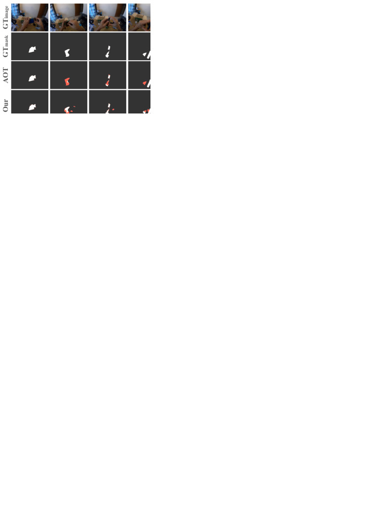
Figure 7: Performance breakdown w.r.t. video length. We show performance comparison of AOT [43] and our method on subsets of different video lengths. We observe that 1) performance decreases in long duration scenarios, demonstrating the complexity in long videos, and 2) our method generally outperforms AOT [43] on long-range subsets, especially upto $10\%$ on videos longer than $34$ secs. # video denotes the number of videos.

In the main paper, we evaluate across various subsets of validation data to measure capability of the model across different aspects of the problem, which includes long videos (LNG) and small objects (SM) subsets. To further demonstrate our model’s performance in these challenging scenarios, we provide a breakdown of results on the subsets at a granular level. The results on small objects (SM) subset is shown in Fig. 6, where we plot $\mathcal{J}_{\text{tr}}$ scores on different object size ranges (as a percentage of the frame size). We observe that performance decreases as object size decreases, dropping from $\sim 65$ to as low as $25$ with objects smaller than $0.2\%$ of the frame size, further confirming the complexity of the task. However, we note that our model consistently outperforms the prior best model, AOT [43], across all subsets, highlighting the effectiveness of our multi-scale object tracking design.

Additionally, the results based on video length subsets is shown in Fig. 7, illustrating the $\mathcal{J}_{\text{tr}}$ scores on different video length ranges. Notably, while the model demonstrates strong performance in shorter videos (i.e., less than $16$ sec), tracking objects becomes challenging in longer setting, with performance (in $\mathcal{J}_{\text{tr}}$-score) dropping from $43$ to $17$ in videos longer than $40$ sec (or containing more than $200$ frames). Despite this, our model outperforms AOT by $\sim 10\%$ in longer video setting (i.e., video length between $34$ and $40$ sec) - confirming the effectiveness of our clip-based memory and matching strategies in long-range scenarios.

8.2 Additional ablation studies

Idx	Bank size	Clip length	$\mathcal{J}_{\text{tr}}$	$\mathcal{J}$
(1)	9	1	35.5	47.4
(2)	9	2	37.7	49.3
(3)	9	3	32.7	44.2
(4)	9	4	32.8	44.7

Table 6: Performance w.r.t. clip lengths during inference. We observe a peak in distribution of performance w.r.t. clip lengths during inference. This suggests that while larger clip lengths (going from $1$ to $2$) allow for accommodating context from longer time spans, it leads to decrease in performance with further increase ($2+$) as information at granular time-scale is lost. Bold number denotes the best performance.

Idx	Bank size	Clip length	$\mathcal{J}_{\text{tr}}$	$\mathcal{J}$
(1)	7	2	36.2	48.2
(2)	8	2	36.2	48.1
(3)	9	2	37.7	49.3
(4)	10	2	36.2	48.2
(5)	11	2	36.4	48.9
(6)	12	2	35.4	47.8

Table 7: Performance w.r.t. bank size during inference. We observe a peak in performance w.r.t. bank sizes. This suggests that, on one hand, increase in bank size leads to increase in model’s capacity to perform matching with more number of elements in memory (or longer-context) which translates to increase in performance. But, on the other hand, we observe decrease in performance upon further increase in bank size, suggesting that since the model was not trained on larger bank sizes, it fails to effectively utilize them. Bold number denotes the best performance.

Memory ablations.

In Section 3.4, we introduced the memory module implemented as a FIFO (first-in-first-out) queue, initially populated with the features of the frame and the ground-truth mask from the initial reference frame. During training, due to computational limitations, we set the memory bank size to 7 and clip-length of 2 for the memory module. However, during inference, when gradients are not computed, we have more GPU memory at our disposal, allowing us to expand the bank size and utilize smaller clip-lengths to include more frames in memory, potentially improving predictions [32]. Note that we apply linear interpolation on RTE to expand it accordingly for larger bank size. Hence, in this subsection, we delve into the impact of employing different bank sizes and clip lengths for the memory module during inference. The corresponding results are presented in Tab. 6 and Tab. 7. In Tab. 6, we observe a performance decrease as clip length increases, corroborating the observations made by a prior clip-based method PCVOS [29]. This suggests that larger clip lengths might enable tracking global features across lengthy videos, but it entails less frequent update to the memory possibly compromising the tracking. On the other hand, the results from testing with different bank sizes are shown in Tab. 7. We observe a slight increase in performance from increasing the bank size from $7$ to $9$, but decrease in performance with the further increase. This suggests that enabling the model to include more frames in memory during inference results in increase in model’s capacity to perform more accurate matching over longer-contexts, but reaches a peak in performance as the model was not trained on larger bank sizes to effectively use them.

Transformation-aware loss ablations.

Method	Re-weighting	$\mathcal{J}_{\text{tr}}$	$\mathcal{J}$
Baseline	-	34.6	46.1
(1)	Connected components	35.4	46.3
(2)	Center of mass	34.9	45.2
(3)	Masked area	36.5	48.2

Table 8: Performance w.r.t. different re-weighting methods used in transformation-aware loss. During training, we compute weights (or importance) of each frame while computing total loss using different methods: 1) Connected components: weights proportional to relative change in the number of connected components, 2) Center of mass: weights proportional to relative change in center of mass, and 3) Masked area: weights proportional to relative change in area of foreground objects. We observe best performance when re-weighting our loss with the Masked Area method.

Method	Re-weighting		$\mathcal{J}_{\text{tr}}$	$\mathcal{J}$
	Dice loss	Focal loss
Baseline			34.6	46.1
(1)	✓		33.2	45.4
(2)		✓	36.5	48.2
(3)	✓	✓	33.4	46.0

Table 9: Performance w.r.t. reweighting combinations of Dice and Focal segmentation loss. We observe best performance when reweighting Focal loss (case 2) only, which we use as a default setting for all our experiments.

As mentioned in Section 3.5, we compute weights for each frame in the proposed re-weighting objective in different ways. Specifically, we explored three different methods: connected components, center of mass, and masked area. For the masked area, we compute the changes in the foreground area of the binary masks. For the center of mass, we calculate the changes in the relative center of mass. The relative center of mass is calculated as the center of the foreground binary mask, considering the top-left corner of the mask as the origin.. Lastly, for the connected components method, we employ OpenCV tools to identify the number of distinct groups or regions within the mask. The results of these approaches are presented in Tab. 8. Notably, simply using the change in the masked area as the weights in the proposed objective yielded the most improvement, resulting in $\sim 2\%$ boost for both $\mathcal{J}^{\text{mean}}$ and $\mathcal{J}_{\text{tr}}^{\text{mean}}$. Based on this observation, we adopted the use of masked area as the default method for computing the weights in our experiments.

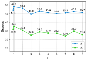
Figure 8: Performance w.r.t. different $\tau$ used in the transformation-aware reweighting. We observe peak in performance ($\mathcal{J}_{\text{tr}}$) at $\tau=1.0$, which we use as a default setting for all our experiments.

Additionally, we note that our transformation-aware re-weighting strategy can be applied to individual or different combinations of the component segmentationlosses (DICE [27] and Focal [25]) computed at the frame-level. We observe in Tab. 9 that applying re-weighting only to the Focal loss yields the best performance. Therefore, in our experiments, we use re-weighting on the focal loss alone as the default setting to achieve optimal performance.

Lastly, in our novel re-weighting loss we introduced a parameter, denoted as $\tau$, in the normalization process. This parameter allows us to control the smoothness of the weights assigned to each frame. In Fig. 8, we empirically assess the effectiveness of different values of $\tau$. We observe that smaller values of $\tau$ result in higher performance. However, when $\tau$ falls below 1.0, the weights become overly sharp, causing a decrease in performance. Note that the larger the value of $\tau$ the smoother the weights become. Based on these results, we used $\tau=1.0$ as our default setting for the re-weighting loss.

8.3 Additional qualitative results

Figure 9: Qualitative comparison on VOST for different model ablations. Best viewed in color; red indicates incorrect predictions.

VOST.

Figure 10: Qualitative results on VISOR. Best viewed in color; red indicates incorrect predictions.

We conduct a qualitative ablation of our proposed approach in Fig. 9. When comparing our model’s performance (third row) and that without multi-scale (or single-scale) matching (last row), we observe that performing matching on a single-scale allows the model to locate the object of interest. However, it struggles to perform precise segmentation, resulting in false positives.

Additionally, when comparing our model (third row), ours without RTE (fourth row) and ours without re-weighting (fifth row), we notice that the baselines fail to track the object after transformations. This leads to false positives again, e.g., from confusing a wristband for a chili. Conversely, our best model adeptly captures the chili without confusion even after the chili is cut, thereby confirming the effectiveness of our design in video object segmentation, particularly in handling transformations.

VISOR.

To illustrate our prediction results on VISOR, we provide qualitative results in Fig. 10. In this example, the target video contains 6 objects of interest with different appearance and size. Our model is able to, not only track all objects without confusion, but also capture the objects with tiny size. This demonstrates the effectiveness of our model in challenging scenarios.

8.4 Additional Visualization and Analysis

Multi-scale matching

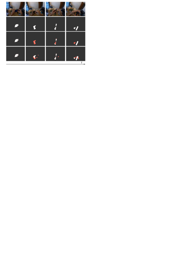
Figure 11: Visualization of the attention maps in the multi-scale matching modules. Scale 1 has a resolution of $\frac{1}{32}$ of the input frame, and scale 2 is at $\frac{1}{16}$ resolution. Best viewed in color; lighter colors indicate higher attention scores. The red box in the first frame denotes the object of interest in the query frame.

We visualize our multi-scale matching on VOST in Fig. 11. For the top-side results, we select a video with multiple instances. Traditional approaches, which only consider matching on a single scale (i.e., scale 1), may struggle when dealing with objects with similar visual appearances at coarse feature maps. This limitation is evident in the matching attention results at scale 1, where the model might confuse different onions and fail to distinguish between them. In contrast, our multi-scale design, depicted in the scale 2 matching attention results, enables the model to capture subtle visual differences between two onions, focusing more accurately on the correct onion.

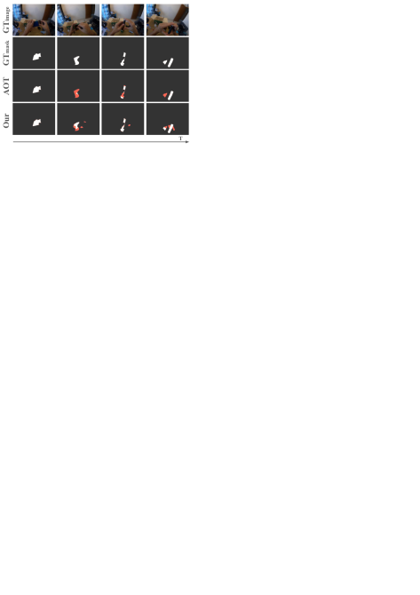
Figure 12: Visualization of Transformation-aware reweighting.

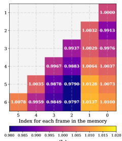
Figure 13: Visualization of RTE. Value in each grid represents the learned importance score for each frame w.r.t. different number of frames in the memory ($n$). Lighter colors indicate higher scores.

Figure 14: Failure case. Best viewed in color; red indicates incorrect predictions.

For the bottom-side results, we select a video with small instances. In the last attention map results, the model struggles to match the object on the coarse features (scale 1), confusing the object of interest with the human hand and other objects. However, in finer features (scale 2) matching, it successfully attends to the object of interest (the herbs being cut). These findings illustrate that our multi-scale matching not only allows the model to capture smaller objects but also potentially prevents the model from confusing objects with similar visual appearance.

Transformation-aware re-weighting

In Section 3.5 in the main submission, we propose the transformation-aware re-weighting to enable the model to place greater emphasis on objects during transformations. In this subsection, we provide examples of training data along with the calculated weights $w^{t}$ for re-weighting to illustrate how this mechanism operates in practical scenarios. These results are showcased in Fig. 12. The figure depicts a video sequence where a person starts cutting an eggplant in the second frame, leading to a significant change in the foreground mask’s area. Our designed re-weighting strategy calculates weights for each frame based on these observed area changes. The weights, displayed in the first row, highlight the highest peak occurring in the second frame, aligning to the frame with the highest degree in object transformation. Consequently, applying these computed weights to re-weight the loss enables us to focus on frames where objects undergo complex transformations.

Relative Time Encoding

As outlined in Section 3.2 in the main submission, our multi-scale matching encoder integrates relative-time-encoding (RTE) to discern the significance of each frame within the memory. In this subsection, we present a qualitative demonstration of the learned embeddings in RTE, depicted in Fig. 13. The results showcase the outcomes obtained using element-wise multiplication in Eq. 3. As for the results in Fig. 13, we re The findings in both figures illustrate how our RTE highlights the importance of frames during the matching module. Notably, the results reveal that the matching of the current frame heavily relies on its neighboring frames compared to those further away in the sequence. Furthermore, regardless of the number of frames in the memory, the first couple of frames in the memory always hold significance, as it represents the ground truth mask and its neighbouring frame.

8.5 Limitation and failure cases

While our method excels in video object segmentation with object shape and appearance transformations, yet it still faces various challenges as follows: (1) Object moves out of frame: In our video demonstration (“video$\_$demo.mp4”), there is a scenario where the object of interest temporarily moves out of the field of view. Our model, like prior methods such as AOT, struggles to successfully track the object upon its return. When the object is out of view, methods relying on matching the current frame with previous frames encounter difficulties in retrieving it due to the lack of the object presence in the frame history. (2) Object occlusion: We illustrate this type of failure in Fig. 14. In this figure, a worker is spreading cement, and our model, along with other methods, can track both the shovel and cement initially. However, once the shovel obstructs the view of the cement in the subsequent frames, the models lose track of the cement and can only track the shovel. Occlusion events like this, pose challenges for current video object segmentation approaches. These cases present significant challenges for existing video object segmentation methodologies. We leave these directions for future research.

9 Societal impact

Semi-automatic video object segmentation has multiple positive societal impacts as it can be used for a variety of useful applications, e.g. robot manipulation and augmented/virtual reality. The ability to track and segment objects in a class agnostic manner can be used in such application areas to enable better human interaction with the environment and improve the user experience. The ability to track under complex transformations is crucial when deploying in the wild in these applications.

However, as with many artificial intelligence algorithms, segmentation and tracking can have negative societal impacts, e.g., through application to target tracking in military systems. To some extent, movements are emerging to limit such applications, e.g. pledges on the part of researchers to ban the use of artificial intelligence in weaponry systems. We have participated in signing that pledge and are supporters of its enforcement through international laws.

References

- Athar et al. [2022] Ali Athar, Jonathon Luiten, Alexander Hermans, Deva Ramanan, and Bastian Leibe. Hodor: High-level object descriptors for object re-segmentation in video learned from static images. In CVPR, 2022.
- Ba et al. [2016] Jimmy Lei Ba, Jamie Ryan Kiros, and Geoffrey E Hinton. Layer normalization. arXiv preprint arXiv:1607.06450, 2016.
- Bao et al. [2018] Linchao Bao, Baoyuan Wu, and Wei Liu. Cnn in mrf: Video object segmentation via inference in a cnn-based higher-order spatio-temporal mrf. In CVPR, 2018.
- Caelles et al. [2017] Sergi Caelles, Kevis-Kokitsi Maninis, Jordi Pont-Tuset, Laura Leal-Taixé, Daniel Cremers, and Luc Van Gool. One-shot video object segmentation. In CVPR, 2017.
- Carion et al. [2020] Nicolas Carion, Francisco Massa, Gabriel Synnaeve, Nicolas Usunier, Alexander Kirillov, and Sergey Zagoruyko. End-to-end object detection with transformers. In ECCV, 2020.
- Cheng et al. [2022] Bowen Cheng, Ishan Misra, Alexander G Schwing, Alexander Kirillov, and Rohit Girdhar. Masked-attention mask transformer for universal image segmentation. In CVPR, 2022.
- Cheng and Schwing [2022] Ho Kei Cheng and Alexander G Schwing. Xmem: Long-term video object segmentation with an atkinson-shiffrin memory model. In ECCV, 2022.
- Cheng et al. [2014] Ming-Ming Cheng, Niloy J Mitra, Xiaolei Huang, Philip HS Torr, and Shi-Min Hu. Global contrast based salient region detection. TPAMI, 2014.
- Damen et al. [2022] Dima Damen, Hazel Doughty, Giovanni Maria Farinella, , Antonino Furnari, Jian Ma, Evangelos Kazakos, Davide Moltisanti, Jonathan Munro, Toby Perrett, Will Price, and Michael Wray. Rescaling egocentric vision: Collection, pipeline and challenges for epic-kitchens-100. International Journal of Computer Vision (IJCV), 130:33–55, 2022.
- Darkhalil et al. [2022] Ahmad Darkhalil, Dandan Shan, Bin Zhu, Jian Ma, Amlan Kar, Richard Higgins, Sanja Fidler, David Fouhey, and Dima Damen. Epic-kitchens visor benchmark: Video segmentations and object relations. In NeurIPS, 2022.
- Deng et al. [2009] Jia Deng, Wei Dong, Richard Socher, Li-Jia Li, Kai Li, and Li Fei-Fei. Imagenet: A large-scale hierarchical image database. In CVPR, 2009.
- Everingham et al. [2010] Mark Everingham, Luc Van Gool, Christopher KI Williams, John Winn, and Andrew Zisserman. The pascal visual object classes (voc) challenge. IJCV, 2010.
- Hariharan et al. [2011] Bharath Hariharan, Pablo Arbeláez, Lubomir Bourdev, Subhransu Maji, and Jitendra Malik. Semantic contours from inverse detectors. In ICCV, 2011.
- He et al. [2016] Kaiming He, Xiangyu Zhang, Shaoqing Ren, and Jian Sun. Deep residual learning for image recognition. In CVPR, 2016.
- Hendrycks and Gimpel [2016] Dan Hendrycks and Kevin Gimpel. Gaussian error linear units (gelus). arXiv preprint arXiv:1606.08415, 2016.
- Hong et al. [2023] Lingyi Hong, Wenchao Chen, Zhongying Liu, Wei Zhang, Pinxue Guo, Zhaoyu Chen, and Wenqiang Zhang. Lvos: A benchmark for long-term video object segmentation. In ICCV, 2023.
- Hu et al. [2018] Yuan-Ting Hu, Jia-Bin Huang, and Alexander G Schwing. Videomatch: Matching based video object segmentation. In ECCV, 2018.
- Jabri et al. [2020] Allan Jabri, Andrew Owens, and Alexei Efros. Space-time correspondence as a contrastive random walk. In NeurIPS, 2020.
- Jampani et al. [2017] Varun Jampani, Raghudeep Gadde, and Peter V Gehler. Video propagation networks. In CVPR, 2017.
- Jang and Kim [2017] Won-Dong Jang and Chang-Su Kim. Online video object segmentation via convolutional trident network. In CVPR, 2017.
- Kim et al. [2023] Donggyun Kim, Jinwoo Kim, Seongwoong Cho, Chong Luo, and Seunghoon Hong. Universal few-shot learning of dense prediction tasks with visual token matching. In ICLR, 2023.
- Liang et al. [2020] Yongqing Liang, Xin Li, Navid Jafari, and Jim Chen. Video object segmentation with adaptive feature bank and uncertain-region refinement. In NeurIPS, 2020.
- Lin et al. [2014] Tsung-Yi Lin, Michael Maire, Serge Belongie, James Hays, Pietro Perona, Deva Ramanan, Piotr Dollár, and C Lawrence Zitnick. Microsoft coco: Common objects in context. In ECCV, 2014.
- Lin et al. [2017a] Tsung-Yi Lin, Piotr Dollár, Ross Girshick, Kaiming He, Bharath Hariharan, and Serge Belongie. Feature pyramid networks for object detection. In CVPR, 2017a.
- Lin et al. [2017b] Tsung-Yi Lin, Priya Goyal, Ross Girshick, Kaiming He, and Piotr Dollár. Focal loss for dense object detection. In ICCV, 2017b.
- Loshchilov and Hutter [2017] Ilya Loshchilov and Frank Hutter. Decoupled weight decay regularization. arXiv preprint arXiv:1711.05101, 2017.
- Milletari et al. [2016] Fausto Milletari, Nassir Navab, and Seyed-Ahmad Ahmadi. V-net: Fully convolutional neural networks for volumetric medical image segmentation. In 3DV, 2016.
- Oh et al. [2019] Seoung Wug Oh, Joon-Young Lee, Ning Xu, and Seon Joo Kim. Video object segmentation using space-time memory networks. In ICCV, 2019.
- Park et al. [2022] Kwanyong Park, Sanghyun Woo, Seoung Wug Oh, In So Kweon, and Joon-Young Lee. Per-clip video object segmentation. In CVPR, 2022.
- Perazzi et al. [2016] Federico Perazzi, Jordi Pont-Tuset, Brian McWilliams, Luc Van Gool, Markus Gross, and Alexander Sorkine-Hornung. A benchmark dataset and evaluation methodology for video object segmentation. In CVPR, 2016.
- Pont-Tuset et al. [2017] Jordi Pont-Tuset, Federico Perazzi, Sergi Caelles, Pablo Arbeláez, Alex Sorkine-Hornung, and Luc Van Gool. The 2017 davis challenge on video object segmentation. arXiv preprint arXiv:1704.00675, 2017.
- Press et al. [2021] Ofir Press, Noah A Smith, and Mike Lewis. Train short, test long: Attention with linear biases enables input length extrapolation. arXiv preprint arXiv:2108.12409, 2021.
- Shi et al. [2015] Jianping Shi, Qiong Yan, Li Xu, and Jiaya Jia. Hierarchical image saliency detection on extended cssd. 2015.
- Tokmakov et al. [2023] Pavel Tokmakov, Jie Li, and Adrien Gaidon. Breaking the” object” in video object segmentation. In CVPR, 2023.
- Vaswani et al. [2017] Ashish Vaswani, Noam Shazeer, Niki Parmar, Jakob Uszkoreit, Llion Jones, Aidan N Gomez, Łukasz Kaiser, and Illia Polosukhin. Attention is all you need. In NeurIPS, 2017.
- Voigtlaender and Leibe [2017] Paul Voigtlaender and Bastian Leibe. Online adaptation of convolutional neural networks for video object segmentation. arXiv preprint arXiv:1706.09364, 2017.
- Voigtlaender et al. [2019] Paul Voigtlaender, Yuning Chai, Florian Schroff, Hartwig Adam, Bastian Leibe, and Liang-Chieh Chen. Feelvos: Fast end-to-end embedding learning for video object segmentation. In CVPR, 2019.
- Xiao et al. [2018] Huaxin Xiao, Jiashi Feng, Guosheng Lin, Yu Liu, and Maojun Zhang. Monet: Deep motion exploitation for video object segmentation. In CVPR, 2018.
- Xu et al. [2018] Ning Xu, Linjie Yang, Yuchen Fan, Jianchao Yang, Dingcheng Yue, Yuchen Liang, Brian Price, Scott Cohen, and Thomas Huang. Youtube-vos: Sequence-to-sequence video object segmentation. In ECCV, 2018.
- Yang et al. [2022] Antoine Yang, Antoine Miech, Josef Sivic, Ivan Laptev, and Cordelia Schmid. Tubedetr: Spatio-temporal video grounding with transformers. In CVPR, 2022.
- Yang et al. [2018] Linjie Yang, Yanran Wang, Xuehan Xiong, Jianchao Yang, and Aggelos K Katsaggelos. Efficient video object segmentation via network modulation. In CVPR, 2018.
- Yang et al. [2020] Zongxin Yang, Yunchao Wei, and Yi Yang. Collaborative video object segmentation by foreground-background integration. In ECCV, 2020.
- Yang et al. [2021a] Zongxin Yang, Yunchao Wei, and Yi Yang. Associating objects with transformers for video object segmentation. In NeurIPS, 2021a.
- Yang et al. [2021b] Zongxin Yang, Yunchao Wei, and Yi Yang. Collaborative video object segmentation by multi-scale foreground-background integration. TPAMI, 2021b.
- Yu et al. [2023] Jiangwei Yu, Xiang Li, Xinran Zhao, Hongming Zhang, and Yu-Xiong Wang. Video state-changing object segmentation. In ICCV, 2023.
- Zhou et al. [2022] Tianfei Zhou, Fatih Porikli, David J Crandall, Luc Van Gool, and Wenguan Wang. A survey on deep learning technique for video segmentation. TPAMI, 2022.