The Effective Horizon Explains Deep RL
Performance in Stochastic Environments

Abstract

Reinforcement learning (RL) theory has largely focused on proving minimax sample complexity bounds. These require strategic exploration algorithms that use relatively limited function classes for representing the policy or value function. Our goal is to explain why deep RL algorithms often perform well in practice, despite using random exploration and much more expressive function classes like neural networks. Our work arrives at an explanation by showing that many stochastic MDPs can be solved by performing only a few steps of value iteration on the random policy’s Q function and then acting greedily. When this is true, we find that it is possible to separate the exploration and learning components of RL, making it much easier to analyze. We introduce a new RL algorithm, SQIRL, that iteratively learns a near-optimal policy by exploring randomly to collect rollouts and then performing a limited number of steps of fitted-Q iteration over those rollouts. We find that any regression algorithm that satisfies basic in-distribution generalization properties can be used in SQIRL to efficiently solve common MDPs. This can explain why deep RL works with complex function approximators like neural networks, since it is empirically established that neural networks generalize well in-distribution. Furthermore, SQIRL explains why random exploration works well in practice, since we show many environments can be solved by effectively estimating the random policy’s Q-function and then applying zero or a few steps of value iteration. We leverage SQIRL to derive instance-dependent sample complexity bounds for RL that are exponential only in an “effective horizon” of lookahead—which is typically much smaller than the full horizon—and on the complexity of the class used for function approximation. Empirically, we also find that SQIRL performance strongly correlates with PPO and DQN performance in a variety of stochastic environments, supporting that our theoretical analysis is predictive of practical performance.

1 Introduction

The theory of reinforcement learning (RL) does not quite predict the practical successes (and failures) of deep RL. Specifically, there are two gaps between theory and practice. First, RL theoreticians focus on strategic exploration, while most deep RL algorithms explore randomly (e.g., they initialize from the random policy or use $\epsilon$-greedy exploration). Explaining why random exploration works in practice is difficult because theorists can show that randomly exploring algorithms’ worst-case sample complexity is exponential in the horizon. Thus, most recent progress in the theory of RL has focused on strategic exploration algorithms, which use upper confidence bound (UCB) bonuses to effectively explore the state space of an environment. Second, RL theory struggles to explain why deep RL can learn efficiently while using complex function approximators like deep neural networks. This is because UCB-type algorithms only work in highly-structured environments where they can use simple function classes to represent value functions and policies.

Our goal is to bridge these two gaps: to explain why random exploration works despite being exponentially bad in the worst-case, and to understand why deep RL succeeds despite using deep neural networks for function approximation. Some recent progress has been made on the former problem by Laidlaw et al. (2023), who analyze when random exploration will succeed in deterministic environments. Their analysis begins by demonstrating a surprising property: in many deterministic environments, it is optimal to act greedily according to the Q-function of the policy that takes actions uniformly at random. This inspires their definition of a property of deterministic environments called the “effective horizon,” which is roughly the number of lookahead steps a Monte Carlo planning algorithm needs to solve the environment when relying on random rollouts to evaluate leaf nodes. They then show that a randomly exploring RL algorithm called Greedy Over Random Policy (GORP) has sample complexity exponential only in the effective horizon rather than the full horizon. While the effective horizon is sometimes equal to the full horizon, they show it is much smaller for many benchmark environments where deep RL succeeds; conversely, when the effective horizon is high, deep RL rarely works.

In this work, we take inspiration from the effective horizon to analyze RL in stochastic environments with function approximation. A major challenge of understanding RL in this setting is the complex interplay between exploration and function approximation. This has made strategic exploration algorithms based on upper confidence bound (UCB) bonuses difficult to analyze because the bonuses must be carefully propagated through the function approximators. The same issue makes it hard to understand deep RL algorithms, in which the current exploration policy affects the data the function approximators are trained on, which in turn affects future exploration. Our idea is to leverage the effective horizon assumption—that limited lookahead followed by random rollouts is enough to arrive at the optimal action—to separate exploration and learning in RL.

We introduce a new RL algorithm, SQIRL (shallow Q-iteration via reinforcement learning), that generalizes GORP to stochastic environments. SQIRL iteratively learns a policy by alternating between collecting data through purely random exploration and then training function approximators on the collected data. During the training phase, SQIRL uses regression to estimate the random policy’s Q-function and then fitted Q-iteration to approximate a few steps of value iteration. The advantage of this algorithm is that it only relies on access to a regression oracle that can generalize in-distribution from i.i.d. samples, which we know works even with neural networks. Thus, unlike strategic exploration algorithms which work for only limited function classes, SQIRL helps explain why RL can work with expressive function classes. Furthermore, the way SQIRL leverages the effective horizon property helps explain why RL works in practice using random exploration.

Theoretically, we prove instance-dependent sample complexity bounds for SQIRL that depend on a stochastic version of the effective horizon as well as properties of the regression oracle used. We demonstrate empirically that the effective horizon assumptions are satisfied in many stochastic benchmark environments. Furthermore, we show that a wide variety of function approximators can be used within SQIRL. For instance, our bounds hold for least-squares regression with function classes of finite pseudo-dimension, including linear functions, neural networks, and many others.

To strengthen our claim that SQIRL can often explain why deep RL succeeds while using random exploration and neural networks, we compare its performance to PPO (Schulman et al., 2017) and DQN (Mnih et al., 2015) in over 150 stochastic environments. We implement SQIRL using least-squares neural network regression and evaluate its empirical sample complexity, along with that of PPO and DQN, in sticky-action versions of the BRIDGE environments from Laidlaw et al. (2023). We find that in environments where both PPO and DQN converge to an optimal policy, SQIRL does as well 89% of the time; when both PPO and DQN fail, SQIRL only succeeds 2% of the time. The strong performance of SQIRL in these stochastic environments implies both that the effective horizon of most of the environments is low and that our regression oracle assumption is met by the neural networks used in SQIRL. Furthermore, the strong relationship between the performance of SQIRL and that of deep RL algorithms suggests that deep RL generally succeeds using the same properties.

These empirical results, combined with our theoretical contributions, show that the effective horizon and the SQIRL algorithm can help explain when and why deep RL works even in stochastic environments. There are still some environments in our experiments where SQIRL fails while PPO or DQN succeeds, suggesting lines of inquiry for future research to address. However, we find that SQIRL’s performance is as similar to PPO and DQN as their performance is to each other’s, suggesting that SQIRL and the effective horizon explain a significant amount of deep RL’s performance.

(a) The GORP algorithm.

(b) The SQIRL algorithm.

Figure 1: We introduce the shallow Q-iteration via reinforcement learning (SQIRL) algorithm, which uses random exploration and function approximation to efficiently solve environments with a low stochastic effective horizon. SQIRL is a generalization of the GORP algorithm (Laidlaw et al., 2023) to stochastic environments. In the figure, both algorithms are shown solving the first timestep of a 2-QVI-solvable MDP. The GORP algorithm (left) uses random rollouts to estimate the random policy’s Q-values at the leaf nodes of a “search tree” and then backs up these values to the root node. It is challenging to generalize this algorithm to stochastic environments because both the initial state and transition dynamics are random. This makes it impossible to perform the steps of GORP where it averages over random rollouts and backs up values along deterministic transitions. SQIRL replaces these steps with regression of the random policy’s Q-values at leaf nodes and fitted Q-iteration (FQI) for backing up values, allowing it to efficiently learn in stochastic environments.

2 Setup and Related Work

We consider the setting of an episodic Markov decision process (MDP) with finite horizon. The MDP comprises a horizon $T\in\mathbb{N}$, states $s\in\mathcal{S}$, actions $a\in\mathcal{A}$, initial state distribution $p_{1}(s_{1})$, transitions $p_{t}(s_{t+1}\mid s_{t},a_{t})$, and reward $R_{t}(s_{t},a_{t})$ for $t\in[T]$, where $[n]$ denotes the set $\{1,\dots,n\}$. We assume that $A=|\mathcal{A}|\geq 2$ is finite. While we do not explicitly consider discounted MDPs, our analysis is easily extendable to incorporate a discount rate.

An RL agent interacts with the MDP for a number of episodes, starting from a state $s_{1}\sim p(s_{1})$. At each step $t\in[T]$ of an episode, the agent observes the state $s_{t}$, picks an action $a_{t}$, receives reward $R(s_{t},a_{t})$, and transitions to the next state $s_{t+1}\sim p(s_{t+1},s_{t},a_{t})$. A policy $\pi$ is a set of functions $\pi_{1},\ldots,\pi_{t}:\mathcal{S}\to\Delta(\mathcal{A})$, which defines for each state and timestep a distribution $\pi_{t}(a\mid s)$ over actions. If a policy is deterministic at some state, then with slight abuse of notation we denote $a=\pi_{t}(s)$ to be the action taken by $\pi_{t}$ in state $s$. We assume that the total reward $\sum_{t=1}^{t}R_{t}(s_{t},a_{t})$ is bounded almost surely in $[0,1]$; any bounded reward function can benormalized to satisfy this assumption.

Using a policy to select actions in an MDP induces a distribution over states and actions with $a_{t}\sim\pi_{t}(\cdot\mid s_{t})$. We use $P_{\pi}$ and $E_{\pi}$ to refer to the probability measure and expectation with respect to this distribution for a particular policy $\pi$. We denote a policy’s Q-function $Q^{\pi}_{t}:\mathcal{S}\times\mathcal{A}\to\mathbb{R}$ and value function $V^{\pi}_{t}:\mathcal{S}\to\mathbb{R}$ for each $t\in[T]$, defined as:

$$\textstyle Q^{\pi}_{t}(s,a)=E_{\pi}\left[\sum_{t^{\prime}=t}^{T}R_{t^{\prime}}(s_{t^{\prime}},a_{t^{\prime}})\mid s_{t}=s,a_{t}=a\right]\quad V^{\pi}_{t}(s)=E_{\pi}\left[\sum_{t^{\prime}=t}^{T}R_{t^{\prime}}(s_{t^{\prime}},a_{t^{\prime}})\mid s_{t}=s\right]$$

Let $J(\pi)=E_{s_{1}\sim p(s_{1})}[V^{\pi}_{1}(s_{1})]$ denote the expected return of a policy $\pi$. The objective of an RL algorithm is to find an $\epsilon$-optimal policy, i.e., one such that $J(\pi)\geq J^{*}-\epsilon$ where $J^{*}=\max_{\pi^{*}}J(\pi^{*})$.

Suppose that after interacting with the environment for $n$ timesteps (i.e., counting one episode as $T$ timesteps), an RL algorithm returns a policy $\pi^{n}$. We define the $(\epsilon,\delta)$ sample complexity $N_{\epsilon,\delta}$ of an RL algorithm as the minimum number of timesteps needed to return an $\epsilon$-optimal policy with probability at least $1-\delta$, where the randomness is over the environment and the RL algorithm:

$$\textstyle N_{\epsilon,\delta}=\min\left\{n\in\mathbb{N}\mid\mathbb{P}\left(J(\pi^{n})\geq J^{*}-\epsilon\right)\geq 1-\delta\right\}.$$

2.1 Related work

As discussed in the introduction, most prior work in RL theory has focused finding strategic exploration-based RL algorithms which have minimax regret or sample complexity bounds (Jiang et al., 2017; Azar et al., 2017; Jin et al., 2018; 2019; Sun et al., 2019; Yang et al., 2020; Dong et al., 2020; Domingues et al., 2021), i.e., they perform well in worst-case environments. However, since the worst-case bounds for random exploration are exponential in the horizon (Koenig & Simmons, 1993; Jin et al., 2018), minimax analysis cannot explain why random exploration works well in practice. Furthermore, while strategic exploration has been extended to broader and broader classes of function approximators (Jin et al., 2021; Du et al., 2021; Foster et al., 2021; Chen et al., 2022), even the broadest of these still requires significant linear or low-rank structure in the environment. This also limits the ability of strategic exploration analysis to explain or improve on practical deep RL algorithms that use neural networks to succeed in unstructured environments.

A much smaller set of work has analyzed random exploration (Liu & Brunskill, 2019; Dann et al., 2022) and more general function approximators (Malik et al., 2021) in RL. However, Laidlaw et al. (2023) show that the sample complexity bounds in these papers fail to explain empirical RL performance even in deterministic environments. While Laidlaw et al. (2023)’s effective horizon property does seem to explain deep RL performance in deterministic environments, it remains an open question whether it can be extended to stochastic ones.

The SQIRL algorithm is partially inspired by fitted Q-iteration (FQI) (Ernst et al., 2005). Our sample complexity bounds are proved using similar methods to previous analyses of error propagation in FQI (Antos et al., 2007; Munos & Szepesvári, 2008). While other works have analyzed FQI for planning (Hallak et al., 2023) or model-based RL (Argenson & Dulac-Arnold, 2021), our analysis is novel because it uses FQI in a model-free RL algorithm which leverages the effective horizon assumption to perform well in realistic environments.

3 The Stochastic Effective Horizon and SQIRL

Figure 2: Among sticky-action versions of the MDPs in the Bridge dataset, more than half can be approximately solved by acting greedily with respect to the random policy’s Q-function ($k=1$); many more can be by applying just a few steps of Q-value iteration before acting greedily ($2\leq k\leq 5$). When $k$ is low, we observe that deep RL algorithms like PPO are much more likely to solve the environment.

We now present our main theoretical findings extending the effective horizon property and GORP algorithm to stochastic environments. The effective horizon was motivated in Laidlaw et al. (2023) by a surprising property that the authors show holds in many deterministic MDPs: acting greedily with respect to the Q-function of the random policy, i.e. ${\pi^{\text{rand}}}_{t}(a\mid s)=1/A\quad\forall s,a,t$, gives an optimal policy. Even when this property doesn’t hold, the authors find that apply a few steps of value iteration to the random policy’s Q-function and then acting greedily is often optimal; they call this property $k$-QVI-solvability. To establish a definition of the effective horizon in stochastic environments, we begin by investigating whether this property holds as commonly in stochastic environments.

To define $k$-QVI-solvability, we introduce some notation. One step of Q-value iteration transforms a Q-function $Q$ to $Q^{\prime}=\text{QVI}(Q)$, where

$$\textstyle Q^{\prime}_{t}(s_{t},a_{t})=R_{t}(s_{t},a_{t})+E_{s_{t+1}}\left[\max_{a\in\mathcal{A}}Q_{t+1}\left(s_{t+1},a\right)\right].$$

We also denote by $\Pi(Q)$ the set of policies which act greedily with respect to the Q-function $Q$; that is,

$$\textstyle\Pi\left(Q\right)=\Big{\{}\pi\;\Big{|}\;\forall s,t\quad\pi_{t}(s)\in\arg\max_{a\in\mathcal{A}}Q_{t}(s,a)\Big{\}}.$$

Furthermore, we define a sequence of Q-functions $Q^{1},\dots,Q^{T}$ by letting $Q^{1}=Q^{\pi^{\text{rand}}}$ be the Q-function of the random policy and $Q^{i+1}=\text{QVI}(Q^{i})$.

Definition 3.1 ($k$-QVI-solvable).

We say an MDP is $k$-QVI-solvable for some $k\in[T]$ if every policy in $\Pi(Q^{k})$ is optimal.

If acting greedily on the random policy’s Q-values is optimal, then an MDP is 1-QVI-solvable; $k$-QVI-solvability extends this to cases where value iteration must be applied to the Q-function before acting greedily.

To see if stochastic environments are commonly $k$-QVI-solvable for small values of $k$, we constructed sticky-action versions of the 155 deterministic MDPs in the Bridge dataset (Laidlaw et al., 2023). Sticky actions are a common and effective method for turning deterministic MDPs into stochastic ones (Machado et al., 2018) by introducing a 25% chance at each timestep of repeating the action from the previous timestep, regardless of the new action taken. We analyzed the minimum values of $k$ for which these MDPs are approximately $k$-QVI-solvable, i.e., where one can achieve at least 95% of the optimal return (measured from the minimum return) by acting greedily with respect to $Q^{k}$. The results are shown in Figure 2. Many environments are approximately $k$-QVI-solvable for very low values of $k$; more than half are approximately 1-QVI-solvable. Furthermore, these are the environments where deep RL algorithms like PPO are most likely to find an optimal policy, suggesting that $k$-QVI-solvability is key to deep RL’s success in stochastic environments.

While many of the sticky-action stochastic MDPs created from the Bridge dataset are $k$-QVI-solvable for small $k$, this alone is not enough to guarantee that random exploration can lead to efficient RL. Laidlaw et al. (2023) define the effective horizon by combining $k$ with a measure of how precisely $Q^{k}$ needs to be estimated to act optimally.

Definition 3.2 ($k$-gap).

If an MDP is $k$-QVI-solvable, we define its $k$-gap as

$$\textstyle\Delta_{k}=\inf_{(t,s)\in[T]\times\mathcal{S}}\big{(}\max_{a^{*}\in\mathcal{A}}Q^{k}_{t}(s,a^{*})-\max_{a\not\in\arg\max_{a}Q^{k}_{t}(s,a)}Q^{k}_{t}(s,a)\big{)}.$$

Intuitively, the smaller the $k$-gap, the more precisely an algorithm must estimate $Q^{k}$ in order to act optimally in an MDP which is $k$-QVI-solvable. We can now define the stochastic effective horizon, which we show is closely related to the effective horizon in deterministic environments:

Definition 3.3 (Stochastic effective horizon).

Given $k\in[T]$, define ${\bar{H}}_{k}=k+\log_{A}(1/\Delta_{k}^{2})$ if an MDP is $k$-QVI-solvable and otherwise let ${\bar{H}}_{k}=\infty$. We define the stochastic effective horizon as ${\bar{H}}=\min_{k}{\bar{H}}_{k}$.

Lemma 3.4.

The deterministic effective horizon $H$ is bounded as

$$\textstyle H\leq\min_{k}\left[{\bar{H}}_{k}+\log_{A}O\left(\log\left(TA^{k}\right)\right)\right].$$

Furthermore, if an MDP is $k$-QVI-solvable, then with probability at least $1-\delta$, GORP will return an optimal policy with sample complexity at most $O(kT^{2}A^{{\bar{H}}_{k}}\log\left(TA/\delta\right))$.

We defer all proofs to the appendix. Lemma 3.4 shows that our definition of the stochastic effective horizon is closely related to the deterministic effective horizon definition: it is an upper-bound up to logarithmic factors. Furthermore, it can bound the sample complexity of the GORP algorithm in deterministic environments. The advantage of the stochastic effective horizon definition is that it does not rely on the GORP algorithm, but is rather defined based on basic properties of the MDP; thus, it equally applies to stochastic environments. However, it is still unclear how a low effective horizon can lead to provably efficient RL in stochastic MDPs.

Algorithm 1 The greedy over random policy (GORP) algorithm, used to define the effective horizon in deterministic environments.

1:procedure GORP($k,m{}$)

2:     for $i=1,\ldots,T$ do

3:         for $a_{i:i+k-1}\in\mathcal{A}^{k}$ do

4:               sample $m{}$ episodes following $\pi_{1},\ldots,\pi_{i-1}$, then actions $a_{i:i+k-1}$, and finally ${\pi^{\text{rand}}}$.

5:               $\hat{Q}_{i}(s_{i},a_{i:i+k-1})\leftarrow$ $\frac{1}{m{}}\sum_{j=1}^{m{}}\sum_{t=i}^{T}\gamma^{t-i}R(s_{t}^{j},a_{t}^{j})$.

6:         end for

7:          $\pi_{i}(s_{i})\leftarrow\arg\max_{a_{i}\in\mathcal{A}}$ $\max_{a_{i+1:i+k-1}\in\mathcal{A}^{k-1}}\hat{Q}_{i}(s_{i},a_{i},a_{i+1:i+k-1}).$

8:     end for

9:     return $\pi$

10:end procedure

3.1 SQIRL

To show that the stochastic effective horizon can provide insight into when and why deep RL succeeds, we introduce the shallow Q-iteration via reinforcement learning (SQIRL) algorithm. Recall the two theory-practice divides we aim to bridge: first, understanding why random exploration works in practice despite being exponentially inefficient in theory; and second, explaining why using deep neural networks for function approximation is feasible in practice despite having little theoretical justification. SQIRL is designed to address both of these. It generalizes the GORP algorithm to stochastic environments, giving sample complexity exponential only in the stochastic effective horizon ${\bar{H}}$ rather than the full horizon $T$. It also allows the use of a wide variety of function approximators that only need to satisfy relatively mild conditions; these are satisfied by neural networks and many other function classes.

GORP

The GORP algorithm (Algorithm 1 and Figure 1(a)) is difficult to generalize to the stochastic case because many of its components are specific to deterministic environments. In particlular, GORP learns a sequence of actions that solve a deterministic MDP by simulating a Monte Carlo planning algorithm. At each iteration, it collects $m$ episodes for each $k$-long action sequence by playing the previous learned actions, the $k$-long action sequence, and then sampling from the ${\pi^{\text{rand}}}$. Then, it picks the action sequence with the highest mean return across the $m$ episodes and adds it to the sequence of learned actions.

At first, it seems very difficult to translate GORP to the stochastic setting. It learns an open-loop sequence of actions, while stochastic environments can only be solved by a closed-loop policy. It also relies on being able to repeatedly reach the same states to estimate their Q-values, which in a stochastic MDP is often impossible due to randomness in the transitions.

Regressing the random policy’s Q-function

To understand how we overcome these challenges, start by considering the first iteration of GORP ($i=1$) when $k=1$. In this case, GORP simply estimates the Q-function of the random policy ($Q^{1}=\smash{Q^{\pi^{\text{rand}}}}$) at the start state $s_{1}$ for each action as an empirical average over random rollouts. The difficulty in stochastic environments is that the start state $s_{1}$ is sampled from a distribution $p(s_{1})$ instead of being fixed. How can we precisely estimate $Q^{1}(s_{1},a)$ over a variety of states and actions when we may never sample the same start state twice? Our key insight is to replace an average over random rollouts with regression of the Q-function from samples of the form $(s_{1},a_{1},y)$, where $y=\smash{\sum_{t=1}^{T}R_{t}(s_{t},a_{t})}$. Standard regression algorithms attempt to estimate the conditional mean $E[y\mid s_{1},a_{1}]$. Since in this case $E[y\mid s_{1},a_{1}]=Q^{1}_{1}(s_{1},a_{1})$, if our regression algorithm works well then it should output $\hat{Q}^{1}_{1}\approx Q^{1}_{1}$.

If we can precisely regress $\hat{Q}^{1}_{1}\approx Q^{1}_{1}$, then for most states $s_{1}$ we should have $\arg\max_{a}\hat{Q}^{1}_{1}(s_{1},a)\subseteq\arg\max_{a}Q^{1}_{1}(s_{1},a)$. This, combined with the MDP being 1-QVI-solvable, means that by setting $\pi_{1}(s_{1})\in\arg\max_{a}\hat{Q}^{1}_{1}(s_{1},a)$, i.e., by acting greedily according to $\hat{Q}^{1}_{1}$ for the first timestep, $\pi_{1}$ should take optimal actions most of the time. Furthermore, if we fix $\pi_{1}$ for the remainder of training, then this means there is a fixed distribution over $s_{2}$, meaning we can also regress $\hat{Q}^{1}_{2}\approx Q^{1}_{2}$, and thus learn $\pi_{2}$; then we can repeat this process as in GORP to learn policies $\pi_{3},\dots,\pi_{T}$ for all timesteps.

Extending to $k-1$ steps of Q iteration

While this explains how to extend GORP to stochastic environments when $k=1$, what about when $k>1$? In this case, GORP follows the first action of the $k$-action sequence with the highest estimated return. However, in stochastic environments, it rarely makes sense to consider a fixed $k$-sequence, since generally after taking one action the agent must base its next action the specific state it reached. Thus, again it is unclear how to extend this part of GORP to the stochastic case. To overcome this challenge, we combine two insights. First, we can reformulate picking the (first action of the) action sequence with the highest estimated return as a series of Bellman backups, as shown in Figure 1(a).

Approximating backups with fitted Q iteration

Our second insight is that we can implement these backups in stochastic environments via fitted-Q iteration (Ernst et al., 2005), which estimates $Q^{j}_{t}$ by regressing from samples of the form $(s_{t},a_{t},y)$, where $y=R_{t}(s_{t},a_{t})+\max_{a_{t+1}\in\mathcal{A}}Q^{j-1}_{t+1}(s_{t+1},a_{t+1})$. Thus, we can implement the $k-1$ backups of GORP by performing $k-1$ steps of fitted-Q iteration. This allows us to extend GORP to stochastic environments when $k>1$. Putting together these insights gives the shallow Q-iteration via reinforcement learning (SQIRL) algorithm, which is presented in full as Algorithm 2.

1:procedure SQIRL($k$, $m$, Regress)

2:     for $i=1,\ldots,T$ do

3:         Collect $m$ episodes by following $\pi_{t}$ for $t<i$ and ${\pi^{\text{rand}}}$ thereafter to obtain $\{(s^{j}_{t},a^{j}_{t},y^{j}_{t})\}_{j=1}^{m}$.

4:         $\hat{Q}^{1}_{i+k-1}\leftarrow\textsc{Regress}(\{(s^{j}_{i+k-1},a^{j}_{i+k-1},\sum_{t=i+k-1}^{T}R_{t}(s^{j}_{t},a^{j}_{t}))\}_{j=1}^{m})$.

5:         for $t=i+k-2,\ldots,i$ do

6:              $\hat{Q}^{i+k-t}_{t}\leftarrow\textsc{Regress}(\{(s^{j}_{t},a^{j}_{t},R_{t}(s^{j}_{t},a^{j}_{t})+\max_{a\in\mathcal{A}}\hat{Q}^{i+k-t-1}_{t+1}(s^{j}_{t+1},a))\}_{j=1}^{m})$.

7:         end for

8:         Define $\pi_{i}$ by $\pi_{i}(s)\leftarrow\arg\max_{a}\hat{Q}^{k}_{i}(s,a)$.

9:     end for

10:return $\pi_{1},\ldots,\pi_{T}$.

11:end procedure

Algorithm 2 The shallow Q-iteration via reinforcement learning (SQIRL) algorithm.

Regression assumptions

To implement the regression and FQI steps, SQIRL uses a regression oracle $\textsc{Regress}(\{(s^{j},a^{j},y^{j})_{j=1}^{m}\})$ which takes as input a dataset of tuples $(s^{j},a^{j},y^{j})$ for $j\in[m]$ and outputs a function $\smash{\hat{Q}}:\mathcal{S}\times\mathcal{A}\to[0,1]$ that aims to predict $E[y\mid s,a]$. In order to analyze the sample complexity of SQIRL, we require the regression oracle to satisfy some basic properties, which we formalize in the following assumption.

Assumption 3.5 (Regression oracle conditions).

Suppose the codomain of the regression oracle $\textsc{Regress}(\cdot)$ is $\mathcal{H}$. Define $\mathcal{V}=\{V(s)=\max_{a\in\mathcal{A}}Q(s,a)\mid Q\in\mathcal{H}\}$ as the class of possible value functions induced by outputs of Regress. We assume there are functions $F:(0,1]\to(0,\infty)$ and $G:[1,\infty)\times(0,1]\to(0,\infty)$ such that the following conditions hold.

(Regression)

Let $Q=Q^{1}_{t}$ for any $t\in[T]$. Suppose a dataset $\{(s,a,y)\}_{j=1}^{m}$ is sampled i.i.d. from a distribution $\mathcal{D}$ such that $y\in[0,1]$ almost surely and $E_{\mathcal{D}}[y\mid s,a]=Q(s,a)$. Then with probability greater than $1-\delta$ over the sample,

$$\textstyle E_{\mathcal{D}}\big{[}(\hat{Q}(s,a)-Q(s,a))^{2}\big{]}\leq O(\frac{\log m}{m}F(\delta))\qquad\text{where}\quad\hat{Q}=\textsc{Regress}\big{(}\{(s^{j},a^{j},y^{j})\}_{j=1}^{m}\big{)}.$$

(Fitted Q-iteration)

Let $Q=Q^{i}_{t}$ for any $t\in[T-1]$ and $i\in[k-1]$; define $V(s)=\max_{a\in\mathcal{A}}Q^{i-1}_{t+1}(s,a)$. Suppose a dataset $\{(s,a,s^{\prime})\}_{j=1}^{m}$ is sampled i.i.d. from a distribution $\mathcal{D}$ such that $s^{\prime}\sim p_{t}(\cdot\mid s,a)$. Then with probability greater than $1-\delta$ over the sample, we have for all $\hat{V}\in\mathcal{V}$ uniformly,

$$\textstyle E_{\mathcal{D}}\big{[}(\hat{Q}(s,a)-Q(s,a))^{2}\big{]}^{1/2}\leq\alpha E_{\mathcal{D}}\big{[}(\hat{V}(s^{\prime})-V(s^{\prime}))^{2}\big{]}^{1/2}+O\Big{(}\sqrt{\frac{\log m}{m}G(\alpha,\delta)}\Big{)}$$

$$\qquad\textstyle\text{where}\quad\hat{Q}=\textsc{Regress}(\{(s^{j},a^{j},R_{t}(s^{j},a^{j})+\hat{V^{\prime}}(s^{\prime j}))\}_{j=1}^{m}).$$

While the conditions in Assumption 3.5 may seem complex, they are relatively mild: we show in Appendix A that they are satisfied by a broad class of regression oracles. The first condition simply says that the regression oracle can take i.i.d. unbiased samples of the random policy’s Q-function and accurately estimate it in-distribution. The error must decrease as $\smash{\widetilde{O}(F(\delta)/m)}$ as the sample size $m$ increases for some $F(\delta)$ which depends on the regression oracle. For instance, we will show that least-squares regression over a hypothesis class of pseudo-dimension $d$ dimensions satisfies the first condition with $F(\delta)=\smash{\widetilde{O}(d+\log(1/\delta))}$.

The second condition is a bit more unusual. It controls how error propagates from an approximate value function at timestep $t+1$ to a Q-function estimated via FQI from the value function at timestep $t$. In particular, the assumption requires that the root mean square (RMS) error in the Q-function be at most $\alpha$ times the RMS error in the value function, plus an additional term of $\smash{\widetilde{O}(\sqrt{G(\alpha,\delta)/m})}$ where $G(\alpha,\delta)$ can again depend on the regression oracle used. In linear MDPs, we can show that this condition is also satisfied by linear regression with $\alpha=1$ and $G(1,\delta)=\smash{\widetilde{O}(d+\log(1/\delta))}$.

Given a regression oracle that satisfies Assumption 3.5, we can prove our main theoretical result: the following upper bound on the sample complexity of SQIRL.

Theorem 3.6 (SQIRL sample complexity).

Fix $\alpha\geq 1$, $\delta\in(0,1]$, and $\epsilon\in(0,1]$. Suppose Regress satisfies Assumption 3.5 and let $D=F(\frac{\delta}{kT})+G(\alpha,\frac{\delta}{kT})$. Then if the MDP is $k$-QVI-solvable for some $k\in[T]$, there is a univeral constant $C$ such that SQIRL (Algorithm 2) will return an $\epsilon$-optimal policy with probability at least $1-\delta$ if $m\geq C\frac{kT\alpha^{2(k-1)}A^{k}D}{\Delta_{k}^{2}\epsilon}\log\frac{kT\alpha AD}{\Delta_{k}\epsilon}$. Thus, the sample complexity of SQIRL is

$$N_{\epsilon,\delta}^{\text{SQIRL}}=\widetilde{O}\left(kT^{3}\alpha^{2(k-1)}A^{{\bar{H}}_{k}}D\log(\alpha D)/\epsilon\right).$$ (1)

To understand the bound on the sample complexity of SQIRL given in (1), first compare it to GORP’s sample complexity in Lemma 3.4. Like GORP, SQIRL has sample complexity exponential in only the effective horizon. As we will see, in many cases we can set $\alpha=1$ and $D\asymp d+\log(kT/\delta)$, where $d$ is the pseudo-dimension of the hypothesis class used by the regression oracle. Then, the sample complexity of SQIRL is $\widetilde{O}(kT^{3}A^{{\bar{H}}_{k}}d/\epsilon)$—ignoring log factors, just a $Td/\epsilon$ factor more than the sample complexity of GORP. The additional factor of $d$ is necessary because SQIRL must learn a Q-function that generalizes over many states, while GORP can estimate the Q-values at a single state in deterministic environments. The $1/\epsilon$ dependence on the desired suboptimality is standard for stochastic environments; for instance, see the strategic exploration bounds in Table 1.

Setting	Sample complexity bounds
	Strategic exploration	SQIRL
Tabular MDP	$\widetilde{O}(TSA/\epsilon^{2})$	$\widetilde{O}(kT^{3}SA^{{\bar{H}}_{k}+1}/\epsilon)$
Linear MDP	$\widetilde{O}(T^{2}d^{2}/\epsilon^{2})$	$\widetilde{O}(kT^{3}dA^{{\bar{H}}_{k}}/\epsilon)$
Q-functions with finite pseudo-dimension	—	$\widetilde{O}(k5^{k}T^{3}dA^{{\bar{H}}_{k}}/\epsilon)$

Table 1: A comparison of our bounds for the sample complexity of SQIRL with bounds from the literature on strategic exploration (Azar et al., 2017; Jin et al., 2018; 2021; Chen et al., 2022). SQIRL can solve stochastic MDPs with a sample complexity that is exponential only in the effective horizon ${\bar{H}}_{k}$. Also, since SQIRL only requires a regression oracle that can estimate Q-functions, it can be used with a wide variety of function classes, including any with finite pseudo-dimension. In contrast, it is difficult to extend the bounds for strategic exploration to more general function classes.

Types of regression oracles

In Appendix A, we show that a broad class of regression oracles satisfy Assumption 3.5. This gives sample complexity bounds shown in Table 1 for SQIRL in tabular and linear MDPs, two settings which are well studied in the strategic exploration literature. However, we find that SQIRL can also solve a much broader range of environments than strategic exploration. For instance, if the regression oracle is implemented via least-squares optimization over a hypothesis class with finite pseudo-dimension $d$, and that hypothesis class contains $Q^{1},\ldots,Q^{k}$, then we obtain a $\widetilde{O}(k5^{k}T^{3}dA^{{\bar{H}}_{k}}/\epsilon)$ bound on SQIRL’s sample complexity. In contrast, it has thus far proven intractable to study strategic exploration algorithms in such general environments.

When considering our bounds on SQIRL, note that in realistic cases $k$ is quite small. As shown in Figure 2, many environments can be approximately solved with $k=1$. We also run all experiments in Section 4 with $k\leq 3$. Thus, although SQIRL’s sample complexity is exponential in $k$, in practice this is fine. Overall, our analysis of the SQIRL algorithm shows theoretically why RL can succeed in complex environments while using random exploration and function approximation. We now turn to validating our theoretical insights empirically.

4 Experiments

While our theoretical results strongly suggest that SQIRL and the stochastic effective horizon can explain deep RL performance, we also want to validate these insights empirically. To do so, we implement SQIRL using deep neural networks for the regression oracle and compare its performance to two common deep RL algorithms, PPO (Schulman et al., 2017) and DQN (Mnih et al., 2015). We evaluate the algorithms in sticky-action versions of the Bridge environments from Laidlaw et al. (2023). These environments are a challenging benchmark for RL algorithms because they are stochastic and have high-dimensional states that necessitate neural network function approximation.

In practice, we slightly modify Algorithm 2 for use with deep neural networks. Following standard practice in deep RL, we use a single neural network to regress the Q-function across all timesteps, rather than using a separate Q-network for each timestep. However, we still “freeze” the greedy policy at each iteration (line 8 in Algorithm 2) by storing a copy of the network’s weights from iteration $i$ and using it for acting on timestep $i$ in future iterations. Second, we stabilize training by using a replay buffer to store the data collected from the environment and then sampling batches from it to train the Q-network. Note that neither of these changes the core algorithm: our implementation is still entirely based around iteratively estimating $Q^{k}$ by using regression and fitted-Q iteration.

Algorithm Envs. solved PPO 98 DQN 78 SQIRL 77 GORP 29 Table 2: The number of sticky-action Bridge environments (out of 155) solved by four RL algorithms. Our SQIRL algorithm solves more than 3/4 of the environments that PPO does and roughly as many as DQN. Meanwhile, GORP (Laidlaw et al., 2023) fails in most because it is not designed for stochastic environments.   Algorithms Sample complexity comparison Correl. Median ratio SQIRL PPO 0.80 1.19 SQIRL DQN 0.56 0.85 PPO DQN 0.55 0.56 Table 3: A comparison of the empirical sample complexities of SQIRL, PPO, and DQN in the sticky-action Bridge environments. SQIRL’s sample complexity has higher Spearman correlation with PPO and DQN than they do with each other. Furthermore, SQIRL tends to have just slightly worse sample complexity then PPO and a bit better sample complexity than DQN.

In each environment, we run PPO, DQN, SQIRL, and GORP for 5 million timesteps. We use the Stable-Baselines3 implementations of PPO and DQN (Raffin et al., 2021). During training, we evaluate the latest policy every 10,000 training timesteps for 100 episodes. We also calculate the exact optimal return using the tabular representations of the environments from the Bridge dataset; we modify the tabular representations to add sticky actions and then run value iteration. If the mean evaluation return of the algorithm reaches the optimal return, we consider the algorithm to have solved the environment. We say the empirical sample complexity of the algorithm in the environment is the number of timesteps needed to reach that optimal return.

Figure 3: The empirical sample complexity of SQIRL correlates closely with that of PPO and DQN, suggesting that our theoretical analysis of SQIRL is a powerful tool for understanding when and why deep RL works in stochastic environments.

Since SQIRL takes parameters $k$ and $m$, we need to tune these parameters for each environment. For each $k\in\{1,2,3,4,5\}$, we perform a binary search over values of $m$ to find the smallest value for which SQIRL solves the environment. We also slightly tune the hyperparameters of PPO and DQN; see Appendices C and D for all experiment details and results. We do not claim that SQIRL is as practical as PPO or DQN, since it requires much more hyperparameter tuning; instead, we mainly see SQIRL as a tool for understanding deep RL.

The results of our experiments are shown in Tables 2 and 3 and Figure 3. Table 2 lists the number of environments solved by each algorithm. GORP barely solves any of the sticky-action Bridge environments, validating that our evaluation environments are stochastic enough that function approximation is necessary to solve them. In contrast, we find that SQIRL solves about three-quarters as many environments as PPO and about the same number as DQN. This shows that SQIRL is not simply a useful algorithm in theory—it can solve a wide variety of stochastic environments in practice. It also suggests that the assumptions we introduce in Section 3 hold for RL in realistic environments with neural network function approximation. If the effective horizon was actually high, or if neural networks could not effectively regression the random policy’s Q-function, we would not expect SQIRL to work as well as it does.

Table 2 and Figure 3 compare the empirical sample complexities of PPO, DQN, and SQIRL. In Table 2, we report the Spearman correlation between the sample complexities of each pair of algorithms in the environments they both solve. We find that SQIRL’s sample complexity correlates better with that of PPO and DQN than they correlate with each other. We also report the median ratio of the sample complexities of each pair of algorithms to see if they agree in absolute scale. We find that SQIRL tends to have similar sample complexity to both PPO and DQN; it typically performs slightly better than DQN and slightly worse than PPO. The fact that there is a close match between the performance of SQIRL and deep RL algorithms—when deep RL has low sample complexity, so does SQIRL, and vice versa—suggests that our theoretical explanation for why SQIRL succeeds is also a good explanation for why deep RL succeeds.

Full-length Atari games

Besides the Bridge environments, which have relatively short horizons, we also compared SQIRL to deep RL algorithms in full-length Atari games. We use the standard Atari evaluation setup from Stable-Baselines3 (Raffin et al., 2021), except that we disable episode restart on loss of life as this does not fit into our RL formalism. A comparison of the learning curves for SQIRL, PPO, and DQN is shown in Figure 4.

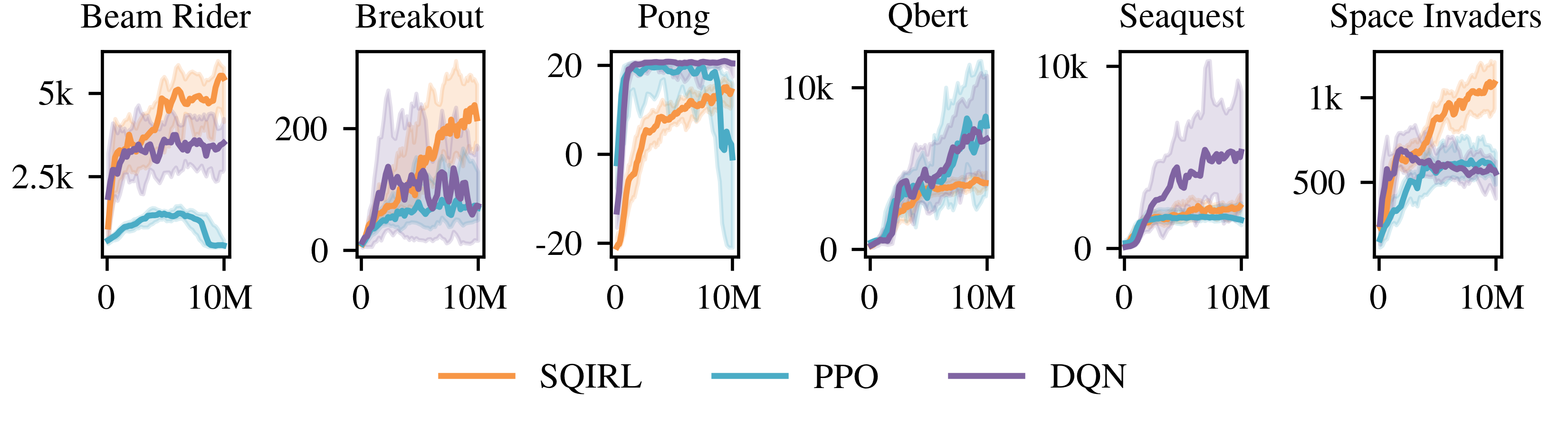
Figure 4: The performance of SQIRL in standard full-length Atari environments is comparable to PPO and DQN. This suggests that PPO and DQN succeed in standard benchmarks for similar reasons that SQIRL succeeds. Thus, our theoretical analysis of SQIRL based on the effective horizon can help explain deep RL performance in these environments.

SQIRL performs comparably to PPO and DQN: it achieves higher reward than both in three of the six games and worse reward than both in only two. This implies that our conclusions from the experiments in the Bridge environments are applicable more broadly: that the stochastic effective horizon is likely low in these environments; that neural networks are able to efficiently regress the Q-function of the random policy; and that these properties lead to the success of deep RL.

5 Conclusion

We have presented theoretical and empirical evidence that SQIRL and the effective horizon can help explain why deep RL succeeds in stochastic environments. Previous theoretical work has not satisfactorily explained why random exploration and complex function approximators should enable efficient RL. However, we leverage regression, fitted Q-iteration, and the low effective horizon assumption to close the theory-practice gap. We hope this paves the way for work that further advances our understanding of deep RL performance or builds improved algorithms based on our analysis.

Appendix

Appendix A Least-squares regression oracles

In this appendix, we prove that many least-squares regression oracles satisfy Assumption 3.5 and thus can be used in SQIRL. These regression oracles minimize the empirical least-squares loss on the training data over some hypothesis class $\mathcal{H}$: $\textsc{Regress}(\{(s^{j},a^{j},y^{j})\}_{j=1}^{m})=\arg\min_{Q\in\mathcal{H}}\frac{1}{m}\sum_{j=1}^{m}(Q(s^{j},a^{j})-y^{j})^{2}$. Proving that Assumption 3.5 is satisfied for such an oracle depends on some basic properties of $\mathcal{H}$. First, we require that $\mathcal{H}$ is of bounded complexity, since otherwise it is impossible to learn a Q-function that generalizes well. We formalize this by requiring a simple bound on the covering number of $\mathcal{H}$:

Definition A.1.

Suppose $\mathcal{H}$ is a hypothesis class of functions $Q:\mathcal{S}\times\mathcal{A}\to[0,1]$. We say $\mathcal{H}$ is a VC-type hypothesis class if for any probability measure $P$ over $\mathcal{S}\times\mathcal{A}$, the $L_{2}(P)$ covering number of $\mathcal{H}$ is bounded as $N(\mathcal{H},L_{2}(P);\epsilon)\leq\left(\frac{B}{\epsilon}\right)^{d}$, where $\|Q-Q^{\prime}\|_{L_{2}(P)}^{2}=E_{P}[\left(Q(s,a)-Q^{\prime}(s,a)\right)^{2}]$.

Many hypothesis classes are VC-type. For instance, if $\mathcal{H}$ has finite pseudo-dimension $d$, then it is VC-type with $d=d$ and $B=O(1)$. If $\mathcal{H}$ is parameterized by $\theta$ in a bounded subset of $\mathbb{R}^{d}$ and $Q^{\theta}$ is Lipschitz in its parameters, then $\mathcal{H}$ is also VC-type with $d=d$ and $B=O(\log(\rho L))$, where $\|\theta\|_{2}\leq\rho$ and $L$ is the Lipschitz constant. See Appendix A.1 for more information.

Besides bounding the complexity of $\mathcal{H}$, we also need it to be rich enough to fit the Q-functions in the MDP. We formalize this in the following two conditions.

Definition A.2.

We say $\mathcal{H}$ is $k$-realizable if for all $i\in[k]$ and $t\in[T]$, $Q^{i}_{t}\in\mathcal{H}$.

Definition A.3.

We say $\mathcal{H}$ is closed under QVI if for any $t\in\{2,\dots,T\}$, $\hat{Q}_{t}\in\mathcal{H}$ implies that $\text{QVI}(\hat{Q}_{t})\in\mathcal{H}$.

Assuming that $\mathcal{H}$ is $k$-realizable is very mild: we would expect that function approximation-based RL would not work at all if the function approximators cannot fit Q-functions in the MDP. The second assumption, that $\mathcal{H}$ is closed under QVI, is more restrictive. However, it turns out this is not necessary for proving that Assumption 3.5 is satisfied; if $\mathcal{H}$ is not closed under QVI, then it just results in slightly worse sample complexity bounds.

Theorem A.4.

Suppose $\mathcal{H}$ is $k$-realizable and of VC-type for constants $B$ and $d$. Then least squares regression over $\mathcal{H}$ satisfies Assumption 3.5 with

$$\textstyle F(\delta) =O\left(d\log(Bd)+\log(1/\delta)\right)$$

$$\textstyle G(\alpha,\delta) =O\left(\left(d\log(ABd/(\alpha-2))+\log(1/\delta)\right)/(\alpha-2)^{4}\right).$$

Furthermore, if $\mathcal{H}$ is also closed under QVI, then we can remove all $(\alpha-2)$ factors in $G$.

Theorem A.4 allows us to immediately bound the sample complexity bounds of SQIRL in a number of settings. For instance, consider a linear MDP with state-action features $\phi(s,a)\in\mathbb{R}^{d}$. We can let $\mathcal{H}=\{\hat{Q}(s,a)=w^{\top}\phi(s,a)\mid w^{\top}\phi(s,a)\in[0,1]\quad\forall(s,a)\in\mathcal{S}\times\mathcal{A}\}$. This hypothesis class is realizable for any $k$, closed under QVI, and of VC-type, meaning SQIRL’s sample complexity is at most $\widetilde{O}(kT^{3}dA^{{\bar{H}}_{k}}/\epsilon)$. Since tabular MDPs are a special case of linear MDPs with $d=SA$, this gives bounds for the tabular case as well. Table 1 shows a comparison between these bounds and previously known bounds for strategic exploration.

However, our analysis can also handle much more general cases than any strategic exploration bounds in the literature. For instance, suppose $\mathcal{H}$ consists of neural networks with $n$ parameters and $\ell$ layers, and say that $\mathcal{H}$ is $k$-realizable, but not necessarily closed under QVI. Then $\mathcal{H}$ has pseudo-dimension of $d=O(n\ell\log(n))$ (Bartlett et al., 2017) and we can bound the sample complexity of SQIRL by $\widetilde{O}(k5^{k}T^{3}n\ell A^{{\bar{H}}_{k}}/\epsilon)$, where we use $\alpha=\sqrt{5}$.

A.1 VC-type hypothesis classes

We now describe two cases when hypothesis classes are of VC-type; thus, by Theorem A.4 these hypothesis classes satisfy Assumption 3.5 and can be used as part of SQIRL.

Example A.5.

We say $\mathcal{H}$ has pseudo-dimension $d$ if the collection of all subgraphs of the functions in $\mathcal{H}$ forms a class of sets with VC dimension $d$. Then by Theorem 2.6.7 of van der Vaart & Wellner (1996), $\mathcal{H}$ is a VC-type class with

$$N(\mathcal{H},L_{2}(P);\epsilon)\leq Cd(16e)^{d}\left(\frac{1}{\epsilon}\right)^{2(d-1)}=O\left(\left(\frac{4e}{\epsilon}\right)^{2d}\right).$$

Example A.6.

Suppose $\mathcal{H}$ is parameterized by $\theta\in\Theta\subseteq\mathbb{R}^{d}$ with $\|\theta\|_{2}\leq B\;\forall\theta$, and $Q_{\theta}(s,a)$ is Lipschitz in $\theta$, i.e.,

$$\left|Q_{\theta}(s,a)-Q_{\theta^{\prime}}(s,a)\right|\leq L\|\theta-\theta^{\prime}\|_{2}\quad\forall\theta,\theta^{\prime}\in\Theta.$$

By Corollary 4.2.13 of Vershynin (2018), the $\epsilon$-covering number of $\{\theta\in\mathbb{R}^{d}\mid\|\theta\|_{2}\leq B\}$ is bounded as $(1+2B/\epsilon)^{d}$. Therefore, the $\epsilon$-packing number of $\mathcal{H}$ is bounded as $(1+4B/\epsilon)^{d}$ (Lemma 4.2.8 of Vershynin (2018)); this in turn implies that the $\epsilon$ packing number of $\Theta$ is bounded identically, since any $\epsilon$-packing of $\Theta$ is also an $\epsilon$-packing of $\mathcal{H}$, which means that the $\epsilon$-covering number of $\Theta$ is also bounded as $(1+4B/\epsilon)^{d}$. If we take $\mathcal{N}_{\epsilon/L}$ to be an $\epsilon/L$-covering of $\Theta$, then for any $Q_{\theta}$, there must be some $\theta^{\prime}\in\mathcal{N}_{\epsilon/L}$ such that $\|\theta-\theta^{\prime}\|_{2}\leq\epsilon/L$, which implies for any probability measure $P$ that

$$\|Q_{\theta}(s,a)-Q_{\theta^{\prime}}(s,a)\|_{L_{2}(P)} =E_{P}\left[\left(Q_{\theta}(s,a)-Q_{\theta^{\prime}}(s,a)\right)^{2}\right]^{1/2}$$

$$\leq E_{P}\left[L^{2}\|\theta-\theta^{\prime}\|_{2}^{2}\right]^{1/2}$$

$$=L\|\theta-\theta^{\prime}\|_{2}\leq\epsilon.$$

Thus $\{Q_{\theta}\mid\theta\in\mathcal{N}_{\epsilon/L}\}$ is an $\epsilon$-covering of $\mathcal{H}$, which implies that the $L_{2}(P)$ covering number of $\mathcal{H}$ is bounded as

$$N(\mathcal{H},L_{2}(P);\epsilon)\leq N(\Theta,L_{2}(P);\epsilon/L)\leq(1+4BL/\epsilon)^{d}=O\left(\left(\frac{4BL}{\epsilon}\right)^{d}\right).$$

Appendix B Proofs

B.1 Proof of Lemma 3.4

See 3.4

Proof.

The bound on $H$ follows immediately from Theorem 5.4 of Laidlaw et al. (2023) by noticing that in our setting, the Q and value functions are always upper-bounded by 1. The bound the sample complexity of GORP then follows from Lemma 5.3 of Laidlaw et al. (2023). ∎

B.2 Proof of Theorem 3.6

To prove our bounds on the sample complexity of SQIRL, we first introduce a series of auxiliary lemmas.

Lemma B.1.

Suppose that an MDP is $k$-QVI solvable and we iteratively find deterministic policies $\pi_{1},\ldots,\pi_{T}$ such that for each $t$, $P_{\pi}(\pi_{t}(s_{t})\not\in\arg\max_{a}Q^{k}_{t}(s_{t},a))\leq\epsilon/T$, where states $s_{t}$ are sampled by following policies $\pi_{1},\ldots,\pi_{t-1}$ for timesteps 1 to $t-1$. Then $\pi$ is $\epsilon$-optimal in the overall MDP, i.e.

$$J(\pi)\geq\max_{\pi^{*}}J(\pi^{*})-\epsilon.$$

Proof.

Let $\mathcal{E}$ denote the event that there is some $t\in[T]$ when $a_{t}\not\in\arg\max_{a}Q^{k}_{t}(s_{t},a)$. By a union bound, we have $P_{\pi}(\mathcal{E})\leq\epsilon$. Now, let $\pi^{*}$ be a policy in $\Pi(Q^{k})$ that agrees with $\pi$ at all states and timesteps where $\pi_{t}(s)\in\arg\max_{a}Q^{k}_{t}(s,a)$. We can write $\tilde{\mathcal{E}}$ as the event that $\exists t\in[T]$, $\pi(s_{t})\neq\pi^{*}(s_{t})$, which is equivalent to $\mathcal{E}$ under the distribution induced by $\pi$. We can now decompose $J(\pi)$ as

$$J(\pi) =E_{\pi}\left[\sum_{t=1}^{T}R_{t}(s_{t},a_{t})\right]$$

$$\geq E_{\pi}\left[\sum_{t=1}^{T}R_{t}(s_{t},a_{t})\mid\neg\mathcal{E}\right]P_{\pi}(\neg\mathcal{E})$$

$$=E_{\pi^{*}}\left[\sum_{t=1}^{T}R_{t}(s_{t},a_{t})\mid\neg\tilde{\mathcal{E}}\right]P_{\pi}(\neg\mathcal{E})$$

$$=E_{\pi^{*}}\left[\sum_{t=1}^{T}R_{t}(s_{t},a_{t})\mid\neg\tilde{\mathcal{E}}\right]P_{\pi}(\neg\mathcal{E})+E_{\pi^{*}}\left[\sum_{t=1}^{T}R_{t}(s_{t},a_{t})\mid\tilde{\mathcal{E}}\right](P_{\pi}(\mathcal{E})-P_{\pi}(\mathcal{E}))$$

$$=E_{\pi^{*}}\left[\sum_{t=1}^{T}R_{t}(s_{t},a_{t})\right]-E_{\pi^{*}}\left[\sum_{t=1}^{T}R_{t}(s_{t},a_{t})\mid\tilde{\mathcal{E}}\right]P_{\pi}(\mathcal{E})$$

$$\geq J(\pi^{*})-\epsilon.$$

∎

Lemma B.2.

Let $\mathcal{D}$ be a distribution over states and actions such that $P_{\mathcal{D}}(a\mid s)=1/A$ for all $s\in\mathcal{S}$, $a\in\mathcal{A}$. Then for any $Q$ and $\hat{Q}:\mathcal{S}\times\mathcal{A}\to[0,1]$, defining $V(s)=\max_{a\in\mathcal{A}}Q(s,a)$ and $\hat{V}$ analogously, we have

$$E_{\mathcal{D}}\left[\left(\hat{V}(s)-V(s)\right)^{2}\right]\leq AE_{\mathcal{D}}\left[\left(\hat{Q}(s,a)-Q(s,a)\right)^{2}\right].$$

Proof.

We have

$$E_{\mathcal{D}}\left[\left(\hat{V}(s)-V(s)\right)^{2}\right] =E_{\mathcal{D}}\left[\left(\max_{a\in\mathcal{A}}\hat{Q}(s,a)-\max_{a\in\mathcal{A}}Q(s,a)\right)^{2}\right]$$

$$\leq E_{\mathcal{D}}\left[\max_{a\in\mathcal{A}}\left(\hat{Q}(s,a)-Q(s,a)\right)^{2}\right]$$

$$\leq E_{\mathcal{D}}\left[\sum_{a\in\mathcal{A}}\left(\hat{Q}(s,a)-Q(s,a)\right)^{2}\right]$$

$$=AE_{\mathcal{D}}\left[\frac{1}{A}\sum_{a\in\mathcal{A}}\left(\hat{Q}(s,a)-Q(s,a)\right)^{2}\right]$$

$$=AE_{\mathcal{D}}\left[\left(\hat{Q}(s,a)-Q(s,a)\right)^{2}\right],$$

where the final equality follows from the fact that $P_{\mathcal{D}}(a\mid s)=1/A$. ∎

Lemma B.3.

Suppose the MDP is $k$-QVI solvable and let $\pi_{i}$ be the policy constructed by stochastic GORP at timestep $i$. Then with probability at least $1-\delta/T$,

$$P_{\pi}\left(\pi_{i}(s)\notin\arg\max_{a}Q^{k}_{i}(s,a)\right)\leq O\left(\frac{\alpha^{2k-2}A^{k}\left(F(\frac{\delta}{kT})+G(\alpha,\frac{\delta}{kT})\right)\log m}{m\Delta_{k}^{2}}\right).$$

Proof.

Let all expectations and probabilities $E$ and $P$ be with respect to the distribution of states and actions induced by following $\pi_{1},\ldots,\pi_{i-1}$ for $t<i$ and ${\pi^{\text{rand}}}$ thereafter. To simplify notation, we write for any $Q_{t},Q^{\prime}_{t}:\mathcal{S}\times\mathcal{A}\to[0,1]$ or $V_{t},V^{\prime}_{t}:\mathcal{S}\to[0,1]$,

$$\left\|Q_{t}-Q^{\prime}_{t}\right\|_{2}^{2} =E\left[\left(Q_{t}(s_{t},a_{t})-Q^{\prime}_{t}(s_{t},a_{t})\right)^{2}\right]$$

$$\left\|V_{t}-V^{\prime}_{t}\right\|_{2}^{2} =E\left[\left(V_{t}(s_{t})-V^{\prime}_{t}(s_{t})\right)^{2}\right].$$

Let $\hat{V}^{i+k-t}_{t}(s)=\max_{a\in\mathcal{A}}\hat{Q}^{i+k-t}_{t}(s,a)$ and $V^{i+k-t}_{t}(s)=\max_{a\in\mathcal{A}}Q^{i+k-t}_{t}(s,a)$. Consider the following three facts:

1. By Assumption 3.5 part 1, with probability at least $1-\delta/(kT)$,

   $$\left\|\hat{Q}^{1}_{i+k-1}-Q^{1}_{i+k-1}\right\|_{2}^{2}\leq C_{1}\frac{F(\frac{\delta}{kT})\log m}{m}.$$

2. By Lemma B.2, for all $t\in\{2,\ldots,k\}$,

   $$\left\|\hat{V}^{i+k-t}_{t}-V^{i+k-t}_{t}\right\|_{2}^{2}\leq A\left\|\hat{Q}^{i+k-t}_{t}-Q^{i+k-t}_{t}\right\|_{2}^{2}.$$

3. By Assumption 3.5 part 2, for any $t\in\{1,\ldots,k-1\}$, with probability at least $1-\delta/(kT)$

   $$\left\|\hat{Q}^{i+k-t}_{t}-Q^{i+k-t}_{t}\right\|_{2}\leq\alpha\left\|\hat{V}^{i+k-t-1}_{t+1}-V^{i+k-t-1}_{t+1}\right\|_{2}+\sqrt{C_{2}\frac{G(\alpha,\frac{\delta}{kT})\log m}{m}}.$$

   Note that it is key that this bound is uniform over all $\hat{V}^{i+k-t-1}_{t+1}\in\mathcal{V}$, since $\hat{V}^{i+k-t-1}_{t+1}$ is estimated based on the same data used to regress $\hat{Q}^{i+k-t}_{t}$.

Via a union bound all of the above facts hold with probability at least $1-\delta/T$. We will combine them to recursively show for $t\in\{1,\ldots,k\}$,

$$\left\|\hat{Q}^{i+k-t}_{t}-Q^{i+k-t}_{t}\right\|_{2}\leq\left(4(\alpha\sqrt{A})^{k-t}-3\right)\sqrt{\frac{D\log m}{m}}\qquad\text{where}\quad D={\textstyle C_{1}F(\frac{\delta}{kT})+C_{2}G(\alpha,\frac{\delta}{kT})}.$$ (2)

The base case $t=k$ is true by fact 1. Now let $t<k$ and assume the above holds for $t+1$. By facts 2 and 3,

$$\left\|\hat{Q}^{i+k-t}_{t}-Q^{i+k-t}_{t}\right\|_{2} \leq\alpha\left\|\hat{V}^{i+k-t-1}_{t+1}-V^{i+k-t-1}_{t+1}\right\|_{2}+\sqrt{C_{2}\frac{G(\alpha,\frac{\delta}{kT})\log m}{m}}$$

$$\leq\alpha\sqrt{A}\left\|\hat{Q}^{i+k-t-1}_{t+1}-Q^{i+k-t-1}_{t+1}\right\|_{2}+\sqrt{C_{2}\frac{G(\alpha,\frac{\delta}{kT})\log m}{m}}$$

$$\leq\alpha\sqrt{A}\left(4(\alpha\sqrt{A})^{k-t-1}-3\right)\sqrt{\frac{D\log m}{m}}+\sqrt{\frac{D\log m}{m}}$$

$$=\left(4(\alpha\sqrt{A})^{k-t}-3\alpha\sqrt{A}+1\right)\sqrt{\frac{D\log m}{m}}$$

$$\leq\left(4(\alpha\sqrt{A})^{k-t}-3\right)\sqrt{\frac{D\log m}{m}},$$

where the last inequality follows from $A\geq 2$ and $\alpha\geq 1$. Thus, by setting $t=i$ in (2), we see that with probability at least $1-\delta/T$,

$$\left\|\hat{Q}^{k}_{i}-Q^{k}_{i}\right\|_{2}^{2}\leq O\left(\frac{\alpha^{2k-2}A^{k-1}\left(F(\frac{\delta}{kT})+G(\alpha,\frac{\delta}{kT})\right)\log m}{m}\right)$$ (3)

$$P_{\pi}(\pi_{i}(s_{i})\notin\arg\max_{a}Q^{k}_{i}(s_{i},a)$$

$$\leq P_{\pi}\left(\arg\max_{a}\hat{Q}^{k}_{i}(s_{i},a)\not\subseteq\arg\max_{a}Q^{k}_{i}(s_{i},a)\right)$$

$$\overset{\text{(i)}}{\leq}P_{\pi}\left(\exists a\in\mathcal{A}\quad\text{s.t.}\quad\left|\hat{Q}^{k}_{i}(s_{i},a)-Q^{k}_{i}(s_{i},a)\right|\geq\Delta_{k}/2\right)$$

$$\leq\sum_{a\in\mathcal{A}}P_{\pi}\left(\left|\hat{Q}^{k}_{i}(s_{i},a)-Q^{k}_{i}(s_{i},a)\right|\geq\Delta_{k}/2\right)$$

$$=A\left(\frac{1}{A}\sum_{a\in\mathcal{A}}P_{\pi}\left(\left|\hat{Q}^{k}_{i}(s_{i},a)-Q^{k}_{i}(s_{i},a)\right|\geq\Delta_{k}/2\right)\right)$$

$$=AP_{\pi}\left(\left|\hat{Q}^{k}_{i}(s_{i},a_{i})-Q^{k}_{i}(s_{i},a_{i})\right|\geq\Delta_{k}/2\right)$$

$$\overset{\text{(ii)}}{\leq}\frac{A}{(\Delta_{k}/2)^{2}}E_{\pi}\left[\left(\hat{Q}^{k}_{i}(s_{i},a_{i})-Q^{k}_{i}(s_{i},a_{i})\right)^{2}\right]$$

$$=\frac{A}{(\Delta_{k}/2)^{2}}\left\|\hat{Q}^{k}_{i}-Q^{k}_{i}\right\|_{2}^{2}$$

$$=O\left(\frac{\alpha^{2k-2}A^{k}\left(F(\frac{\delta}{kT})+G(\alpha,\frac{\delta}{kT})\right)\log m}{m\Delta_{k}^{2}}\right).$$

Here, (i) follows from Definition 3.2 of the $k$-gap and (ii) follows from Markov’s inequality. ∎

See 3.6

Proof.

Given the lower bound on $m$, we can bound

$$\frac{\log m}{m}=O\left(\frac{\Delta_{k}^{2}\epsilon}{T\alpha^{2k-2}A^{k}D}\right).$$

Combining this with Lemma B.3, we see that with probability at least $1-\delta$, for all $i\in[T]$

$$P_{\pi}\left(\pi_{i}(s_{i})\notin\arg\max_{a}Q^{k}_{i}(s_{i},a)\right)\leq\epsilon/T.$$

Thus, by Lemma B.1, $\pi$ is $\epsilon$-optimal in the overall MDP $\mathcal{M}$. ∎

B.3 Proof of Theorem A.4

See A.4

Proof.

Throughout the proof, we will use the notation that $\|Q-Q^{\prime}\|_{2}^{2}=E_{\mathcal{D}}[(Q(s,a)-Q^{\prime}(s,a))^{2}]$ and $\|V-V^{\prime}\|_{2}^{2}=E_{\mathcal{D}}[(V(s^{\prime})-V^{\prime}(s^{\prime}))^{2}]$.

First, we will prove the regression part of Assumption 3.5. To do so, we use results on least-squares regression from Koltchinskii (2006). Note that our definition of VC-type classes coincides with condition (2.1) in Koltchinskii (2006). By combining Example 3 from Section 2.5 and Theorem 13 of Koltchinskii (2006), we have that for any $\bar{Q}(s,a)$ with $\mathbb{E}[y\mid s,a]=\bar{Q}(s,a)$, and for any $\lambda\in(0,1]$,

$$\mathbb{P}\left(\left\|\hat{Q}-\bar{Q}\right\|_{2}^{2}\leq(1+\lambda)\inf_{\tilde{Q}\in\mathcal{H}}\left\|\tilde{Q}-\bar{Q}\right\|_{2}^{2}+O\left(\frac{d}{m\lambda^{2}}\log\left(\frac{Bdm}{\lambda}\right)+\frac{u+1}{\lambda m}\right)\right)\leq\log\left(\frac{em}{u}\right)e^{-u}.$$

$$\text{where}\qquad\hat{Q}=\textsc{Regress}(\{(s^{j},a^{j},y^{j})\}_{j=1}^{m}).$$ (4)

If we set

$$u=\log\left(\frac{e+\log m}{\delta}\right)\geq 1,$$

then the right-hand side of (4) is bounded as

$$\log\left(\frac{em}{u}\right)e^{-u}\leq\log(em)e^{-u}=\log(em)\frac{\delta}{e+\log m}<\delta.$$

Thus, plugging this value of $u$ into (4), we have that with probability at least $1-\delta$,

$$\left\|\hat{Q}-\bar{Q}\right\|_{2}^{2}\leq(1+\lambda)\inf_{\tilde{Q}\in\mathcal{H}}\left\|\tilde{Q}-\bar{Q}\right\|_{2}^{2}+O\left(\frac{d\log\left(\frac{Bdm}{\lambda}\right)+\log\frac{m}{\delta}}{m\lambda^{2}}\right).$$ (5)

For the regression condition of Assumption 3.5, we have $\bar{Q}=Q_{t}^{k}\in\mathcal{H}$. Thus, $\inf_{\tilde{Q}\in\mathcal{H}}\|\tilde{Q}-\bar{Q}\|_{2}^{2}=0$, and we can set $\lambda=1$ in (5) to obtain

$$\left\|\hat{Q}-Q_{t}^{k}\right\|_{2}^{2}\leq O\left(\frac{d\log(Bdm)+\log\frac{m}{\delta}}{m}\right),$$

leading to the desired bound of

$$F(\delta)=O\left(d\log(Bd)+\log\frac{1}{\delta}\right).$$

To the fitted Q-iteration condition of Assumption 3.5, we begin by defining a norm $\rho$ on $\mathcal{V}\times\mathcal{H}$ by

$$\rho\Big{(}(V,Q),(V^{\prime},Q^{\prime})\Big{)}=\max\{\|V-V^{\prime}\|_{2},\|Q-Q^{\prime}\|_{2}\}.$$

Note that since we showed in Lemma B.2 that

$$E_{\mathcal{D}}\left[\left(V(s^{\prime})-V^{\prime}(s^{\prime})\right)^{2}\right]\leq AE_{\mathcal{D},a^{\prime}\sim\text{Unif}(\mathcal{A})}\left[\left(Q(s^{\prime},a^{\prime})-Q^{\prime}(s^{\prime},a^{\prime})\right)^{2}\right]$$

$$\quad\text{where}\quad V(s^{\prime})=\max_{a^{\prime}\in\mathcal{A}}Q(s^{\prime},a^{\prime}),V^{\prime}(s^{\prime})=\max_{a^{\prime}\in\mathcal{A}}Q^{\prime}(s^{\prime},a^{\prime}),$$

this implies that any $\epsilon$-cover of $\mathcal{H}$ is also an $\epsilon\sqrt{A}$-cover of $\mathcal{V}$ with respect to $L_{2}(P)$ for any distribution $P$ over $s^{\prime}$. Thus, by the definition of VC-type classes, we have

$$N(\mathcal{V},L_{2}(\mathcal{D});\epsilon) \leq\left(\frac{B\sqrt{A}}{\epsilon}\right)^{d}$$

$$N(\mathcal{H},L_{2}(\mathcal{D});\epsilon) \leq\left(\frac{B}{\epsilon}\right)^{d}$$

$$N(\mathcal{V}\times\mathcal{H},\rho;\epsilon) \leq\left(\frac{B\sqrt{A}}{\epsilon}\right)^{d}\left(\frac{B}{\epsilon}\right)^{d}\leq\left(\frac{B\sqrt{A}}{\epsilon}\right)^{2d}.$$

Now define $\mathcal{W}\subseteq\mathcal{V}\times\mathcal{H}$ as

$$\mathcal{W}=\left\{(\hat{V},\hat{Q})\in\mathcal{V}\times\mathcal{H}\;\middle|\;\hat{Q}=\textsc{Regress}\left(\left\{(s^{j},a^{j},R_{t}(s^{j},a^{j})+\hat{V}(s^{\prime j}))\right\}_{j=1}^{m}\right)\right\}.$$

By properties of packing and covering numbers, since any $\epsilon$-packing of $\mathcal{W}$ is also an $\epsilon$-packing of $\mathcal{V}\times\mathcal{H}$, we have

$$N(\mathcal{W},\rho;\epsilon)\leq M(\mathcal{W},\rho;\epsilon/2)\leq M(\mathcal{V}\times\mathcal{H},\rho;\epsilon/2)\leq N(\mathcal{V}\times\mathcal{H},\rho;\epsilon/2)\leq\left(\frac{2B\sqrt{A}}{\epsilon}\right)^{2d}.$$

Thus, let $\mathcal{N}_{1/\sqrt{m}}$ be a $1/\sqrt{m}$-covering of $\mathcal{W}$ with size at most $(2B\sqrt{Am})^{2d}$.

Fix any $(\hat{V},\hat{Q})\in\mathcal{N}_{1/\sqrt{m}}$ and define $\bar{Q}(s,a)=E[R_{t}(s,a)+\hat{V}(s^{\prime})\mid s,a]$. Then by an identical argument to (5), with probability at least $1-\delta$, for any $\lambda\in(0,1]$,

$$\left\|\hat{Q}-\bar{Q}\right\|_{2}^{2}\leq(1+\lambda)\inf_{\tilde{Q}\in\mathcal{H}}\left\|\tilde{Q}-\bar{Q}\right\|_{2}^{2}+O\left(\frac{d\log\left(\frac{Bdm}{\lambda}\right)+\log\frac{m}{\delta}}{m\lambda^{2}}\right).$$

We can extend this to a bound on all $(\hat{V},\hat{Q})\in\mathcal{N}_{1/\sqrt{m}}$ by dividing $\delta$ by $|\mathcal{N}_{1/\sqrt{m}}|$ and applying a union bound. Thus, with probability at least $1-\delta$, for all $(\hat{V},\hat{Q})\in\mathcal{N}_{1/\sqrt{m}}$ and any $\lambda\in(0,1]$,

$$\left\|\hat{Q}-\bar{Q}\right\|_{2}^{2} \leq(1+\lambda)\inf_{\tilde{Q}\in\mathcal{H}}\left\|\tilde{Q}-\bar{Q}\right\|_{2}^{2}+O\left(\frac{d\log\left(\frac{Bdm}{\lambda}\right)+d\log(BAm)+\log\frac{m}{\delta}}{m\lambda^{2}}\right)$$

$$=(1+\lambda)\inf_{\tilde{Q}\in\mathcal{H}}\left\|\tilde{Q}-\bar{Q}\right\|_{2}^{2}+O\left(\frac{d\log\left(\frac{BAdm}{\lambda}\right)+\log\frac{m}{\delta}}{m\lambda^{2}}\right).$$

Finally, we extend this to a bound over all $(\hat{V},\hat{Q})\in\mathcal{W}$. For any $(\hat{V},\hat{Q})\in\mathcal{W}$, there must be some $(\hat{V}^{\prime},\hat{Q}^{\prime})\in\mathcal{N}_{1/\sqrt{m}}$ such that $\rho((\hat{V},\hat{Q}),(\hat{V}^{\prime},\hat{Q}^{\prime}))\leq 1/\sqrt{m}$. Let $\bar{Q}^{\prime}(s,a)=E[R_{t}(s,a)+\hat{V}^{\prime}(s^{\prime})\mid s,a]$. Then

$$\|\bar{Q}-\bar{Q}^{\prime}\|_{2}^{2} =E_{\mathcal{D}}\left[\left(\bar{Q}(s,a)-\bar{Q}^{\prime}(s,a)\right)^{2}\right]$$

$$=E_{\mathcal{D}}\left[\left(E_{\mathcal{D}}\left[\hat{V}(s^{\prime})-\hat{V}^{\prime}(s^{\prime})\right]\right)^{2}\right]$$

$$\leq E_{\mathcal{D}}\left[\left(\hat{V}(s^{\prime})-\hat{V}^{\prime}(s^{\prime})\right)^{2}\right]\leq\frac{1}{m},$$

where the second-to-last inequality follows from Jensen’s inequality. Thus, by the triangle inequality,

$$\left\|\hat{Q}-\bar{Q}\right\|_{2} \leq\left\|\hat{Q}-\hat{Q}^{\prime}\right\|_{2}+\left\|\hat{Q}^{\prime}-\bar{Q}^{\prime}\right\|_{2}+\left\|\bar{Q}^{\prime}-\bar{Q}\right\|_{2}$$

$$\leq\left\|\hat{Q}^{\prime}-\bar{Q}^{\prime}\right\|_{2}+\frac{2}{\sqrt{m}}$$

$$\leq\sqrt{1+\lambda}\inf_{\tilde{Q}^{\prime}\in\mathcal{H}}\left\|\tilde{Q}^{\prime}-\bar{Q}^{\prime}\right\|_{2}+O\left(\sqrt{\frac{d\log\left(\frac{BAdm}{\lambda}\right)+\log\frac{m}{\delta}}{m\lambda^{2}}}\right).$$

for all $(\hat{V},\hat{Q})\in\mathcal{W}$ and any $\lambda\in(0,1]$ with probability at least $1-\delta$.

We now consider the two possible conditions in the theorem. If $\mathcal{H}$ is both $k$-realizable and closed under QVI, then this implies $\bar{Q}^{\prime}\in\mathcal{H}$ for all $(\hat{V}^{\prime},\hat{Q}^{\prime})\in\mathcal{N}_{1/\sqrt{m}}$, meaning $\inf_{\tilde{Q}^{\prime}\in\mathcal{H}}\|\tilde{Q}^{\prime}-\bar{Q}^{\prime}\|_{2}=0$. Thus, we can set $\lambda=1$ in the above bound to obtain

$$\left\|\hat{Q}-Q\right\|_{2} \leq\left\|\bar{Q}-Q\right\|_{2}+\left\|\hat{Q}-\bar{Q}\right\|_{2}$$

$$\leq\left\|\hat{V}-V\right\|_{2}+O\left(\sqrt{\frac{d\log\left(\frac{BAdm}{\lambda}\right)+\log\frac{m}{\delta}}{m\lambda^{2}}}\right),$$

showing that the FQI condition of Assumption 3.5 holds with

$$G(\alpha,\delta)=O\Big{(}d\log(BAd)+\log(1/\delta)\Big{)}.$$

Otherwise, if $\mathcal{H}$ is only $k$-realizable, then this implies $Q\in\mathcal{H}$. Thus,

$$\inf_{\tilde{Q}^{\prime}\in\mathcal{H}}\left\|\tilde{Q}^{\prime}-\bar{Q}^{\prime}\right\|_{2}\leq\left\|Q-\bar{Q}^{\prime}\right\|_{2}\leq\left\|V-\hat{V}\right\|_{2}+\frac{1}{\sqrt{m}}.$$

This implies that

$$\left\|\hat{Q}-Q\right\|_{2} \leq\left\|\bar{Q}-Q\right\|_{2}+\left\|\hat{Q}-\bar{Q}\right\|_{2}$$

$$\leq\left\|\hat{V}-V\right\|_{2}+\sqrt{1+\lambda}\left\|V-\hat{V}\right\|_{2}+\frac{1}{\sqrt{m}}+O\left(\sqrt{\frac{d\log\left(\frac{BAdm}{\lambda}\right)+\log\frac{m}{\delta}}{m\lambda^{2}}}\right)$$

$$\leq(2+\sqrt{\lambda})\left\|\hat{V}-V\right\|_{2}+O\left(\sqrt{\frac{d\log\left(\frac{BAdm}{\lambda}\right)+\log\frac{m}{\delta}}{m\lambda^{2}}}\right).$$

Setting $\alpha=2+\sqrt{\lambda}$ shows that the FQI condition of Assumption 3.5 holds with

$$G(\alpha,\delta)=O\left(\frac{d\log\left(\frac{BAd}{\alpha-2}\right)+\log\frac{1}{\delta}}{(\alpha-2)^{4}}\right).$$

∎

Appendix C Experiment details

In this appendix, we describe details of the experiments from Section 4. We use the implementations of PPO and DQN from Stable-Baselines3 (Raffin et al., 2021), and in general use their hyperparameters which have been optimized for Atari games. For network archictures, we use convolutional neural nets similar to those used by Mnih et al. (2015). We use a discount rate of $\gamma=1$ for the Atari and Procgen environments in Bridge but $\gamma=0.99$ for the MiniGrid environments, as otherwise we found that RL completely failed.

PPO

We use the following hyperparameters for PPO:

Hyperparameter	Value
Training timesteps	5,000,000
Rollout length	$\{128,1280\}$
SGD minibatch size	256
SGD epochs per iteration	4
Optimizer	Adam
Learning rate	$2.5\times 10^{-4}$
GAE coefficient ($\lambda$)	0.95
Entropy coefficient	0.01
Clipping parameter	0.1
Value function coefficient	0.5

Table 4: Hyperparameters we use for PPO.

For each environment, we try rollout lengths of 128 and 1280 as we found this was the most important parameter to tune.

DQN

We use the following hyperparameters for DQN:

Hyperparameter	Value
Training timesteps	5,000,000
Timesteps before learning starts	0
Replay buffer size	100,000
Target network update frequency	8,000
Final $\epsilon$	0.01
SGD minibatch size	32
Env. steps per gradient step	4
Optimizer	Adam
Learning rate	$10^{-4}$

Table 5: Hyperparameters we use for DQN.

We try decaying the $\epsilon$ value for $\epsilon$-greedy over the course of either 500 thousand or 5 million timesteps, as we found this was the most sensitive hyperparameter to tune for DQN.

SQIRL

We use the following hyperparameters for SQIRL:

Hyperparameter	Value
Training timesteps	5,000,000
Replay buffer size	1,000,000
$k$	{1, 2, 3}
SGD minibatch size	128
SGD epochs per iteration	10
Optimizer	Adam
Learning rate	$10^{-4}$

Table 6: Hyperparameters we use for SQIRL.

As we describe in the main text, we run SQIRL with $k\in\{1,2,3,4,5\}$ and tune $m$ via binary search.

For the full-horizon Atari experiments, we also tune $k\in\{1,2,3,4,5\}$ and use $m=10$ for all the games, except for Qbert, where we use $m=20$. We run 5 random seeds and plot the median and range of evaluation returns—that is, returns from running the current greedy policy for 20 episodes every 100,000 training steps.

Appendix D Full results

D.1 Table of empirical sample complexities

This table lists the empirical sample complexities of PPO, DQN, SQIRL, and GORP.

	PPO	DQN	SQIRL	GORP
$\textsc{Alien}_{10}$	$3.34\times 10^{6}$	$4.82\times 10^{6}$	$>5\times 10^{6}$	$>5\times 10^{6}$
$\textsc{Amidar}_{20}$	$>5\times 10^{6}$	$>5\times 10^{6}$	$>5\times 10^{6}$	$>5\times 10^{6}$
$\textsc{Assault}_{10}$	$1.00\times 10^{4}$	$2.80\times 10^{5}$	$1.00\times 10^{4}$	$1.00\times 10^{5}$
$\textsc{Asterix}_{10}$	$2.00\times 10^{5}$	$2.10\times 10^{5}$	$2.50\times 10^{5}$	$5.40\times 10^{6}$
$\textsc{Asteroids}_{10}$	$>5\times 10^{6}$	$>5\times 10^{6}$	$>5\times 10^{6}$	$>5\times 10^{6}$
$\textsc{Atlantis}_{10}$	$6.00\times 10^{4}$	$1.00\times 10^{5}$	$1.00\times 10^{4}$	$1.60\times 10^{5}$
$\textsc{Atlantis}_{20}$	$3.40\times 10^{5}$	$>5\times 10^{6}$	$1.46\times 10^{6}$	$>5\times 10^{6}$
$\textsc{Atlantis}_{30}$	$>5\times 10^{6}$	$>5\times 10^{6}$	$>5\times 10^{6}$	$>5\times 10^{6}$
$\textsc{Atlantis}_{40}$	$>5\times 10^{6}$	$>5\times 10^{6}$	$>5\times 10^{6}$	$>5\times 10^{6}$
$\textsc{Atlantis}_{50}$	$>5\times 10^{6}$	$>5\times 10^{6}$	$>5\times 10^{6}$	$>5\times 10^{6}$
$\textsc{Atlantis}_{70}$	$>5\times 10^{6}$	$>5\times 10^{6}$	$>5\times 10^{6}$	$>5\times 10^{6}$
$\textsc{BankHeist}_{10}$	$8.60\times 10^{5}$	$4.40\times 10^{6}$	$3.01\times 10^{6}$	$>5\times 10^{6}$
$\textsc{BattleZone}_{10}$	$1.30\times 10^{5}$	$2.29\times 10^{6}$	$2.80\times 10^{5}$	$>5\times 10^{6}$
$\textsc{BeamRider}_{20}$	$>5\times 10^{6}$	$4.43\times 10^{6}$	$>5\times 10^{6}$	$>5\times 10^{6}$
$\textsc{Bowling}_{30}$	$6.30\times 10^{5}$	$>5\times 10^{6}$	$>5\times 10^{6}$	$3.63\times 10^{6}$
$\textsc{Breakout}_{10}$	$8.00\times 10^{4}$	$8.00\times 10^{4}$	$4.00\times 10^{4}$	$1.00\times 10^{4}$
$\textsc{Breakout}_{20}$	$2.60\times 10^{5}$	$1.01\times 10^{6}$	$1.90\times 10^{5}$	$1.50\times 10^{5}$
$\textsc{Breakout}_{30}$	$2.46\times 10^{6}$	$>5\times 10^{6}$	$2.60\times 10^{5}$	$>5\times 10^{6}$
$\textsc{Breakout}_{40}$	$1.67\times 10^{6}$	$>5\times 10^{6}$	$1.28\times 10^{6}$	$>5\times 10^{6}$
$\textsc{Breakout}_{50}$	$1.22\times 10^{6}$	$>5\times 10^{6}$	$>5\times 10^{6}$	$>5\times 10^{6}$
$\textsc{Breakout}_{70}$	$2.52\times 10^{6}$	$>5\times 10^{6}$	$>5\times 10^{6}$	$>5\times 10^{6}$
$\textsc{Breakout}_{100}$	$2.77\times 10^{6}$	$>5\times 10^{6}$	$>5\times 10^{6}$	$>5\times 10^{6}$
$\textsc{Breakout}_{200}$	$>5\times 10^{6}$	$>5\times 10^{6}$	$>5\times 10^{6}$	$>5\times 10^{6}$
$\textsc{Centipede}_{10}$	$>5\times 10^{6}$	$>5\times 10^{6}$	$>5\times 10^{6}$	$>5\times 10^{6}$
$\textsc{ChopperCommand}_{10}$	$>5\times 10^{6}$	$3.36\times 10^{6}$	$>5\times 10^{6}$	$>5\times 10^{6}$
$\textsc{CrazyClimber}_{20}$	$4.00\times 10^{4}$	$1.00\times 10^{4}$	$3.00\times 10^{4}$	$>5\times 10^{6}$
$\textsc{CrazyClimber}_{30}$	$4.20\times 10^{5}$	$1.60\times 10^{5}$	$1.30\times 10^{5}$	$>5\times 10^{6}$
$\textsc{DemonAttack}_{10}$	$2.21\times 10^{6}$	$5.50\times 10^{5}$	$3.01\times 10^{6}$	$>5\times 10^{6}$
$\textsc{Enduro}_{10}$	$4.50\times 10^{5}$	$5.30\times 10^{5}$	$3.84\times 10^{6}$	$>5\times 10^{6}$
$\textsc{FishingDerby}_{10}$	$2.10\times 10^{5}$	$2.05\times 10^{6}$	$>5\times 10^{6}$	$>5\times 10^{6}$
$\textsc{Freeway}_{10}$	$1.00\times 10^{4}$	$2.00\times 10^{4}$	$1.00\times 10^{4}$	$1.00\times 10^{4}$
$\textsc{Freeway}_{20}$	$1.00\times 10^{4}$	$1.00\times 10^{4}$	$1.00\times 10^{4}$	$6.00\times 10^{4}$
$\textsc{Freeway}_{30}$	$2.30\times 10^{5}$	$4.90\times 10^{5}$	$1.21\times 10^{6}$	$>5\times 10^{6}$
$\textsc{Freeway}_{40}$	$2.80\times 10^{5}$	$5.10\times 10^{5}$	$5.30\times 10^{5}$	$>5\times 10^{6}$
$\textsc{Freeway}_{50}$	$4.70\times 10^{5}$	$8.40\times 10^{5}$	$>5\times 10^{6}$	$>5\times 10^{6}$
$\textsc{Freeway}_{70}$	$2.01\times 10^{6}$	$3.63\times 10^{6}$	$>5\times 10^{6}$	$>5\times 10^{6}$
$\textsc{Freeway}_{100}$	$>5\times 10^{6}$	$>5\times 10^{6}$	$>5\times 10^{6}$	$>5\times 10^{6}$
$\textsc{Freeway}_{200}$	$>5\times 10^{6}$	$>5\times 10^{6}$	$>5\times 10^{6}$	$>5\times 10^{6}$
$\textsc{Frostbite}_{10}$	$9.00\times 10^{4}$	$5.50\times 10^{5}$	$2.40\times 10^{5}$	$6.40\times 10^{5}$
$\textsc{Gopher}_{30}$	$1.40\times 10^{5}$	$6.10\times 10^{5}$	$1.00\times 10^{5}$	$4.70\times 10^{5}$
$\textsc{Gopher}_{40}$	$>5\times 10^{6}$	$>5\times 10^{6}$	$>5\times 10^{6}$	$>5\times 10^{6}$
$\textsc{Hero}_{10}$	$3.00\times 10^{4}$	$7.00\times 10^{4}$	$1.00\times 10^{4}$	$1.52\times 10^{6}$
$\textsc{IceHockey}_{10}$	$6.00\times 10^{4}$	$1.65\times 10^{6}$	$9.10\times 10^{5}$	$>5\times 10^{6}$
$\textsc{Kangaroo}_{20}$	$>5\times 10^{6}$	$>5\times 10^{6}$	$>5\times 10^{6}$	$>5\times 10^{6}$
$\textsc{Kangaroo}_{30}$	$>5\times 10^{6}$	$>5\times 10^{6}$	$>5\times 10^{6}$	$>5\times 10^{6}$
$\textsc{MontezumaRevenge}_{15}$	$>5\times 10^{6}$	$>5\times 10^{6}$	$>5\times 10^{6}$	$>5\times 10^{6}$
$\textsc{MsPacman}_{20}$	$>5\times 10^{6}$	$>5\times 10^{6}$	$>5\times 10^{6}$	$>5\times 10^{6}$
$\textsc{NameThisGame}_{20}$	$1.50\times 10^{5}$	$6.30\times 10^{5}$	$2.60\times 10^{5}$	$>5\times 10^{6}$
$\textsc{Phoenix}_{10}$	$8.20\times 10^{5}$	$4.85\times 10^{6}$	$>5\times 10^{6}$	$>5\times 10^{6}$
$\textsc{Pong}_{20}$	$6.00\times 10^{5}$	$1.10\times 10^{5}$	$5.90\times 10^{5}$	$>5\times 10^{6}$
$\textsc{Pong}_{30}$	$4.70\times 10^{5}$	$3.50\times 10^{5}$	$3.59\times 10^{6}$	$>5\times 10^{6}$
$\textsc{Pong}_{40}$	$>5\times 10^{6}$	$>5\times 10^{6}$	$>5\times 10^{6}$	$>5\times 10^{6}$
$\textsc{Pong}_{50}$	$>5\times 10^{6}$	$>5\times 10^{6}$	$>5\times 10^{6}$	$>5\times 10^{6}$
$\textsc{Pong}_{70}$	$>5\times 10^{6}$	$>5\times 10^{6}$	$>5\times 10^{6}$	$>5\times 10^{6}$
$\textsc{Pong}_{100}$	$>5\times 10^{6}$	$>5\times 10^{6}$	$>5\times 10^{6}$	$>5\times 10^{6}$
$\textsc{PrivateEye}_{10}$	$1.20\times 10^{5}$	$1.90\times 10^{5}$	$7.00\times 10^{4}$	$1.29\times 10^{6}$
$\textsc{Qbert}_{10}$	$1.60\times 10^{5}$	$3.73\times 10^{6}$	$2.00\times 10^{4}$	$>5\times 10^{6}$
$\textsc{Qbert}_{20}$	$5.60\times 10^{5}$	$>5\times 10^{6}$	$>5\times 10^{6}$	$>5\times 10^{6}$
$\textsc{RoadRunner}_{10}$	$1.50\times 10^{5}$	$1.97\times 10^{6}$	$3.10\times 10^{5}$	$5.22\times 10^{6}$
$\textsc{Seaquest}_{10}$	$2.00\times 10^{4}$	$2.80\times 10^{5}$	$1.00\times 10^{4}$	$>5\times 10^{6}$
$\textsc{Skiing}_{10}$	$>5\times 10^{6}$	$>5\times 10^{6}$	$>5\times 10^{6}$	$>5\times 10^{6}$
$\textsc{SpaceInvaders}_{10}$	$6.40\times 10^{5}$	$2.40\times 10^{5}$	$4.00\times 10^{4}$	$8.60\times 10^{5}$
$\textsc{Tennis}_{10}$	$>5\times 10^{6}$	$1.29\times 10^{6}$	$>5\times 10^{6}$	$>5\times 10^{6}$
$\textsc{TimePilot}_{10}$	$1.00\times 10^{5}$	$7.30\times 10^{5}$	$4.00\times 10^{4}$	$5.80\times 10^{5}$
$\textsc{Tutankham}_{10}$	$7.70\times 10^{5}$	$3.81\times 10^{6}$	$2.09\times 10^{6}$	$>5\times 10^{6}$
$\textsc{VideoPinball}_{10}$	$>5\times 10^{6}$	$1.70\times 10^{6}$	$7.10\times 10^{5}$	$1.14\times 10^{6}$
$\textsc{WizardOfWor}_{20}$	$>5\times 10^{6}$	$>5\times 10^{6}$	$>5\times 10^{6}$	$>5\times 10^{6}$
$\textsc{Bigfish}_{10}^{\text{E0}}$	$>5\times 10^{6}$	$4.60\times 10^{5}$	$>5\times 10^{6}$	$>5\times 10^{6}$
$\textsc{Bigfish}_{10}^{\text{E1}}$	$3.20\times 10^{5}$	$3.00\times 10^{5}$	$1.10\times 10^{5}$	$>5\times 10^{6}$
$\textsc{Bigfish}_{10}^{\text{E2}}$	$1.30\times 10^{6}$	$5.70\times 10^{5}$	$1.57\times 10^{6}$	$>5\times 10^{6}$
$\textsc{Bigfish}_{10}^{\text{H0}}$	$>5\times 10^{6}$	$4.20\times 10^{5}$	$1.78\times 10^{6}$	$>5\times 10^{6}$
$\textsc{Chaser}_{20}^{\text{E0}}$	$1.90\times 10^{5}$	$>5\times 10^{6}$	$>5\times 10^{6}$	$>5\times 10^{6}$
$\textsc{Chaser}_{20}^{\text{E1}}$	$>5\times 10^{6}$	$>5\times 10^{6}$	$>5\times 10^{6}$	$>5\times 10^{6}$
$\textsc{Chaser}_{20}^{\text{E2}}$	$1.70\times 10^{5}$	$>5\times 10^{6}$	$>5\times 10^{6}$	$>5\times 10^{6}$
$\textsc{Chaser}_{20}^{\text{H0}}$	$>5\times 10^{6}$	$>5\times 10^{6}$	$>5\times 10^{6}$	$>5\times 10^{6}$
$\textsc{Climber}_{10}^{\text{E0}}$	$7.00\times 10^{4}$	$4.70\times 10^{5}$	$5.00\times 10^{4}$	$>5\times 10^{6}$
$\textsc{Climber}_{10}^{\text{E1}}$	$8.00\times 10^{4}$	$>5\times 10^{6}$	$7.00\times 10^{4}$	$4.00\times 10^{4}$
$\textsc{Climber}_{10}^{\text{E2}}$	$4.40\times 10^{5}$	$>5\times 10^{6}$	$1.29\times 10^{6}$	$>5\times 10^{6}$
$\textsc{Climber}_{10}^{\text{H0}}$	$>5\times 10^{6}$	$>5\times 10^{6}$	$>5\times 10^{6}$	$>5\times 10^{6}$
$\textsc{Coinrun}_{10}^{\text{E0}}$	$>5\times 10^{6}$	$>5\times 10^{6}$	$5.15\times 10^{6}$	$4.60\times 10^{6}$
$\textsc{Coinrun}_{10}^{\text{E1}}$	$1.18\times 10^{6}$	$>5\times 10^{6}$	$7.40\times 10^{5}$	$>5\times 10^{6}$
$\textsc{Coinrun}_{10}^{\text{E2}}$	$9.90\times 10^{5}$	$>5\times 10^{6}$	$>5\times 10^{6}$	$>5\times 10^{6}$
$\textsc{Coinrun}_{10}^{\text{H0}}$	$1.00\times 10^{4}$	$2.00\times 10^{4}$	$1.00\times 10^{4}$	$1.90\times 10^{5}$
$\textsc{Dodgeball}_{10}^{\text{E0}}$	$3.50\times 10^{5}$	$1.90\times 10^{5}$	$7.10\times 10^{5}$	$>5\times 10^{6}$
$\textsc{Dodgeball}_{10}^{\text{E1}}$	$6.20\times 10^{5}$	$1.00\times 10^{6}$	$1.26\times 10^{6}$	$>5\times 10^{6}$
$\textsc{Dodgeball}_{10}^{\text{E2}}$	$2.60\times 10^{5}$	$1.54\times 10^{6}$	$1.20\times 10^{5}$	$6.90\times 10^{5}$
$\textsc{Dodgeball}_{10}^{\text{H0}}$	$6.70\times 10^{5}$	$2.59\times 10^{6}$	$1.43\times 10^{6}$	$>5\times 10^{6}$
$\textsc{Fruitbot}_{40}^{\text{E0}}$	$>5\times 10^{6}$	$4.80\times 10^{5}$	$>5\times 10^{6}$	$>5\times 10^{6}$
$\textsc{Fruitbot}_{40}^{\text{E1}}$	$1.52\times 10^{6}$	$3.77\times 10^{6}$	$>5\times 10^{6}$	$>5\times 10^{6}$
$\textsc{Fruitbot}_{40}^{\text{E2}}$	$6.60\times 10^{5}$	$4.00\times 10^{4}$	$5.00\times 10^{4}$	$>5\times 10^{6}$
$\textsc{Fruitbot}_{40}^{\text{H0}}$	$>5\times 10^{6}$	$>5\times 10^{6}$	$>5\times 10^{6}$	$>5\times 10^{6}$
$\textsc{Heist}_{10}^{\text{E1}}$	$5.70\times 10^{5}$	$1.65\times 10^{6}$	$>5\times 10^{6}$	$>5\times 10^{6}$
$\textsc{Jumper}_{10}^{\text{H0}}$	$>5\times 10^{6}$	$>5\times 10^{6}$	$>5\times 10^{6}$	$>5\times 10^{6}$
$\textsc{Jumper}_{20}^{\text{E0}}$	$1.00\times 10^{4}$	$>5\times 10^{6}$	$1.00\times 10^{4}$	$1.00\times 10^{4}$
$\textsc{Jumper}_{20}^{\text{E1}}$	$1.00\times 10^{4}$	$>5\times 10^{6}$	$1.00\times 10^{4}$	$1.00\times 10^{4}$
$\textsc{Jumper}_{20}^{\text{E2}}$	$1.90\times 10^{5}$	$>5\times 10^{6}$	$2.60\times 10^{5}$	$>5\times 10^{6}$
$\textsc{Jumper}_{20}^{\text{EX}}$	$>5\times 10^{6}$	$>5\times 10^{6}$	$>5\times 10^{6}$	$>5\times 10^{6}$
$\textsc{Leaper}_{20}^{\text{E1}}$	$>5\times 10^{6}$	$>5\times 10^{6}$	$>5\times 10^{6}$	$>5\times 10^{6}$
$\textsc{Leaper}_{20}^{\text{E2}}$	$2.20\times 10^{6}$	$>5\times 10^{6}$	$>5\times 10^{6}$	$>5\times 10^{6}$
$\textsc{Leaper}_{20}^{\text{H0}}$	$>5\times 10^{6}$	$>5\times 10^{6}$	$>5\times 10^{6}$	$>5\times 10^{6}$
$\textsc{Leaper}_{20}^{\text{EX}}$	$>5\times 10^{6}$	$>5\times 10^{6}$	$>5\times 10^{6}$	$>5\times 10^{6}$
$\textsc{Maze}_{30}^{\text{E0}}$	$1.00\times 10^{4}$	$>5\times 10^{6}$	$2.00\times 10^{4}$	$1.00\times 10^{4}$
$\textsc{Maze}_{30}^{\text{E1}}$	$>5\times 10^{6}$	$>5\times 10^{6}$	$>5\times 10^{6}$	$>5\times 10^{6}$
$\textsc{Maze}_{30}^{\text{E2}}$	$2.00\times 10^{4}$	$>5\times 10^{6}$	$1.00\times 10^{4}$	$1.00\times 10^{4}$
$\textsc{Maze}_{30}^{\text{H0}}$	$2.83\times 10^{6}$	$>5\times 10^{6}$	$>5\times 10^{6}$	$>5\times 10^{6}$
$\textsc{Maze}_{100}^{\text{EX}}$	$>5\times 10^{6}$	$>5\times 10^{6}$	$>5\times 10^{6}$	$>5\times 10^{6}$
$\textsc{Miner}_{10}^{\text{E0}}$	$2.90\times 10^{5}$	$>5\times 10^{6}$	$1.60\times 10^{5}$	$>5\times 10^{6}$
$\textsc{Miner}_{10}^{\text{E1}}$	$1.30\times 10^{5}$	$3.40\times 10^{5}$	$1.20\times 10^{5}$	$>5\times 10^{6}$
$\textsc{Miner}_{10}^{\text{E2}}$	$4.00\times 10^{4}$	$2.87\times 10^{6}$	$1.00\times 10^{4}$	$5.20\times 10^{5}$
$\textsc{Miner}_{10}^{\text{H0}}$	$4.00\times 10^{5}$	$5.30\times 10^{5}$	$4.50\times 10^{5}$	$>5\times 10^{6}$
$\textsc{Ninja}_{10}^{\text{E0}}$	$5.50\times 10^{5}$	$3.24\times 10^{6}$	$2.76\times 10^{6}$	$>5\times 10^{6}$
$\textsc{Ninja}_{10}^{\text{E1}}$	$2.09\times 10^{6}$	$>5\times 10^{6}$	$3.76\times 10^{6}$	$>5\times 10^{6}$
$\textsc{Ninja}_{10}^{\text{E2}}$	$>5\times 10^{6}$	$>5\times 10^{6}$	$>5\times 10^{6}$	$>5\times 10^{6}$
$\textsc{Ninja}_{10}^{\text{H0}}$	$>5\times 10^{6}$	$>5\times 10^{6}$	$>5\times 10^{6}$	$>5\times 10^{6}$
$\textsc{Plunder}_{10}^{\text{E0}}$	$3.00\times 10^{4}$	$3.00\times 10^{4}$	$1.00\times 10^{4}$	$1.00\times 10^{5}$
$\textsc{Plunder}_{10}^{\text{E1}}$	$1.00\times 10^{4}$	$3.00\times 10^{4}$	$1.00\times 10^{4}$	$1.00\times 10^{4}$
$\textsc{Plunder}_{10}^{\text{E2}}$	$1.30\times 10^{5}$	$3.70\times 10^{5}$	$3.14\times 10^{6}$	$1.02\times 10^{6}$
$\textsc{Plunder}_{10}^{\text{H0}}$	$1.00\times 10^{4}$	$7.00\times 10^{4}$	$1.00\times 10^{4}$	$3.00\times 10^{4}$
$\textsc{Starpilot}_{10}^{\text{E0}}$	$2.43\times 10^{6}$	$6.70\times 10^{5}$	$2.18\times 10^{6}$	$>5\times 10^{6}$
$\textsc{Starpilot}_{10}^{\text{E1}}$	$4.30\times 10^{5}$	$8.30\times 10^{5}$	$2.02\times 10^{6}$	$>5\times 10^{6}$
$\textsc{Starpilot}_{10}^{\text{E2}}$	$8.30\times 10^{5}$	$1.66\times 10^{6}$	$2.66\times 10^{6}$	$>5\times 10^{6}$
$\textsc{Starpilot}_{10}^{\text{H0}}$	$>5\times 10^{6}$	$2.70\times 10^{6}$	$>5\times 10^{6}$	$>5\times 10^{6}$
Empty-5x5	$1.70\times 10^{5}$	$2.90\times 10^{5}$	$2.80\times 10^{5}$	$1.78\times 10^{6}$
Empty-6x6	$2.40\times 10^{5}$	$3.50\times 10^{5}$	$5.50\times 10^{5}$	$>5\times 10^{6}$
Empty-8x8	$3.20\times 10^{5}$	$3.60\times 10^{5}$	$8.40\times 10^{5}$	$>5\times 10^{6}$
Empty-16x16	$1.01\times 10^{6}$	$>5\times 10^{6}$	$>5\times 10^{6}$	$>5\times 10^{6}$
DoorKey-5x5	$5.80\times 10^{5}$	$8.90\times 10^{5}$	$2.44\times 10^{6}$	$>5\times 10^{6}$
DoorKey-6x6	$1.69\times 10^{6}$	$>5\times 10^{6}$	$>5\times 10^{6}$	$>5\times 10^{6}$
DoorKey-8x8	$>5\times 10^{6}$	$>5\times 10^{6}$	$>5\times 10^{6}$	$>5\times 10^{6}$
DoorKey-16x16	$>5\times 10^{6}$	$>5\times 10^{6}$	$>5\times 10^{6}$	$>5\times 10^{6}$
MultiRoom-N2-S4	$4.20\times 10^{5}$	$5.70\times 10^{5}$	$2.76\times 10^{6}$	$>5\times 10^{6}$
MultiRoom-N4-S5	$>5\times 10^{6}$	$>5\times 10^{6}$	$>5\times 10^{6}$	$>5\times 10^{6}$
MultiRoom-N6	$>5\times 10^{6}$	$>5\times 10^{6}$	$>5\times 10^{6}$	$>5\times 10^{6}$
KeyCorridorS3R1	$9.40\times 10^{5}$	$>5\times 10^{6}$	$>5\times 10^{6}$	$>5\times 10^{6}$
KeyCorridorS3R2	$>5\times 10^{6}$	$>5\times 10^{6}$	$>5\times 10^{6}$	$>5\times 10^{6}$
KeyCorridorS3R3	$4.23\times 10^{6}$	$>5\times 10^{6}$	$>5\times 10^{6}$	$>5\times 10^{6}$
KeyCorridorS4R3	$>5\times 10^{6}$	$>5\times 10^{6}$	$>5\times 10^{6}$	$>5\times 10^{6}$
Unlock	$8.20\times 10^{5}$	$>5\times 10^{6}$	$>5\times 10^{6}$	$>5\times 10^{6}$
UnlockPickup	$>5\times 10^{6}$	$>5\times 10^{6}$	$>5\times 10^{6}$	$>5\times 10^{6}$
BlockedUnlockPickup	$>5\times 10^{6}$	$>5\times 10^{6}$	$>5\times 10^{6}$	$>5\times 10^{6}$
ObstructedMaze-1Dl	$>5\times 10^{6}$	$>5\times 10^{6}$	$>5\times 10^{6}$	$>5\times 10^{6}$
ObstructedMaze-1Dlh	$>5\times 10^{6}$	$>5\times 10^{6}$	$>5\times 10^{6}$	$>5\times 10^{6}$
ObstructedMaze-1Dlhb	$>5\times 10^{6}$	$>5\times 10^{6}$	$>5\times 10^{6}$	$>5\times 10^{6}$
FourRooms	$>5\times 10^{6}$	$>5\times 10^{6}$	$>5\times 10^{6}$	$>5\times 10^{6}$
LavaCrossingS9N1	$6.30\times 10^{5}$	$5.30\times 10^{5}$	$4.73\times 10^{6}$	$>5\times 10^{6}$
LavaCrossingS9N2	$2.27\times 10^{6}$	$6.00\times 10^{5}$	$2.12\times 10^{6}$	$>5\times 10^{6}$
LavaCrossingS9N3	$5.00\times 10^{5}$	$3.50\times 10^{5}$	$1.23\times 10^{6}$	$2.46\times 10^{6}$
LavaCrossingS11N5	$>5\times 10^{6}$	$>5\times 10^{6}$	$>5\times 10^{6}$	$>5\times 10^{6}$
SimpleCrossingS9N1	$4.50\times 10^{5}$	$8.70\times 10^{5}$	$4.43\times 10^{6}$	$>5\times 10^{6}$
SimpleCrossingS9N2	$5.10\times 10^{5}$	$5.40\times 10^{5}$	$>5\times 10^{6}$	$>5\times 10^{6}$
SimpleCrossingS9N3	$3.30\times 10^{5}$	$5.00\times 10^{5}$	$8.10\times 10^{5}$	$>5\times 10^{6}$
SimpleCrossingS11N5	$>5\times 10^{6}$	$>5\times 10^{6}$	$>5\times 10^{6}$	$>5\times 10^{6}$
LavaGapS5	$2.50\times 10^{5}$	$2.80\times 10^{5}$	$4.90\times 10^{5}$	$>5\times 10^{6}$
LavaGapS6	$9.50\times 10^{5}$	$1.48\times 10^{6}$	$1.79\times 10^{6}$	$>5\times 10^{6}$
LavaGapS7	$2.88\times 10^{6}$	$1.62\times 10^{6}$	$3.43\times 10^{6}$	$>5\times 10^{6}$

D.2 Table of returns

This table lists the optimal returns in each sticky-action MDP as well as the highest returns achieved by PPO, DQN, and SQIRL.

	Returns
MDP	Optimal policy	PPO	DQN	SQIRL
$\textsc{Alien}_{10}$	$158.13$	$158.5$	$158.5$	$156.4$
$\textsc{Amidar}_{20}$	$76.49$	$64.76$	$75.29$	$61.67$
$\textsc{Assault}_{10}$	$105.0$	$105.0$	$105.0$	$106.05$
$\textsc{Asterix}_{10}$	$327.53$	$336.5$	$343.5$	$337.0$
$\textsc{Asteroids}_{10}$	$170.81$	$133.3$	$127.3$	$131.5$
$\textsc{Atlantis}_{10}$	$187.5$	$192.0$	$190.0$	$194.0$
$\textsc{Atlantis}_{20}$	$740.91$	$754.0$	$723.0$	$767.0$
$\textsc{Atlantis}_{30}$	$1,829.52$	$1,238.0$	$995.0$	$1,166.0$
$\textsc{Atlantis}_{40}$	$2,620.35$	$1,794.0$	$1,186.0$	$1,746.0$
$\textsc{Atlantis}_{50}$	$4,856.81$	$3,683.0$	$1,865.0$	$3,143.0$
$\textsc{Atlantis}_{70}$	$7,932.88$	$6,108.0$	$3,347.0$	$5,411.0$
$\textsc{BankHeist}_{10}$	$26.15$	$26.3$	$27.1$	$26.3$
$\textsc{BattleZone}_{10}$	$1,497.07$	$1,620.0$	$1,520.0$	$1,590.0$
$\textsc{BeamRider}_{20}$	$129.23$	$126.72$	$129.8$	$125.4$
$\textsc{Bowling}_{30}$	$8.8$	$8.81$	$5.77$	$7.69$
$\textsc{Breakout}_{10}$	$1.17$	$1.41$	$1.21$	$1.32$
$\textsc{Breakout}_{20}$	$1.93$	$1.95$	$1.99$	$2.01$
$\textsc{Breakout}_{30}$	$2.5$	$2.59$	$2.27$	$2.52$
$\textsc{Breakout}_{40}$	$2.61$	$2.7$	$2.21$	$2.64$
$\textsc{Breakout}_{50}$	$2.69$	$2.69$	$2.12$	$2.51$
$\textsc{Breakout}_{70}$	$2.9$	$2.95$	$2.28$	$2.57$
$\textsc{Breakout}_{100}$	$3.08$	$3.12$	$1.9$	$2.56$
$\textsc{Breakout}_{200}$	$3.08$	$2.83$	$0.73$	$2.58$
$\textsc{Centipede}_{10}$	$1,321.17$	$900.0$	$1,213.24$	$1,224.2$
$\textsc{ChopperCommand}_{10}$	$553.42$	$469.0$	$560.0$	$512.0$
$\textsc{CrazyClimber}_{20}$	$324.9$	$334.0$	$326.0$	$332.0$
$\textsc{CrazyClimber}_{30}$	$698.07$	$701.0$	$705.0$	$714.0$
$\textsc{DemonAttack}_{10}$	$37.07$	$37.1$	$38.3$	$37.3$
$\textsc{Enduro}_{10}$	$4.27$	$4.3$	$4.37$	$4.26$
$\textsc{FishingDerby}_{10}$	$7.5$	$7.58$	$7.5$	$6.79$
$\textsc{Freeway}_{10}$	$1.0$	$1.0$	$1.0$	$1.0$
$\textsc{Freeway}_{20}$	$2.0$	$2.0$	$2.0$	$2.0$
$\textsc{Freeway}_{30}$	$3.75$	$3.77$	$3.77$	$3.83$
$\textsc{Freeway}_{40}$	$4.75$	$4.76$	$4.79$	$4.78$
$\textsc{Freeway}_{50}$	$5.75$	$5.81$	$5.76$	$5.72$
$\textsc{Freeway}_{70}$	$8.49$	$8.49$	$8.5$	$8.05$
$\textsc{Freeway}_{100}$	$11.83$	$10.84$	$11.41$	$10.91$
$\textsc{Freeway}_{200}$	$23.84$	$21.53$	$21.99$	$21.68$
$\textsc{Frostbite}_{10}$	$66.72$	$67.9$	$67.5$	$67.4$
$\textsc{Gopher}_{30}$	$18.75$	$19.4$	$19.0$	$19.6$
$\textsc{Gopher}_{40}$	$112.93$	$83.8$	$72.0$	$72.4$
$\textsc{Hero}_{10}$	$74.71$	$75.0$	$75.0$	$75.0$
$\textsc{IceHockey}_{10}$	$1.0$	$1.0$	$1.0$	$1.0$
$\textsc{Kangaroo}_{20}$	$186.32$	$172.0$	$182.0$	$170.0$
$\textsc{Kangaroo}_{30}$	$444.7$	$200.0$	$370.0$	$210.0$
$\textsc{MontezumaRevenge}_{15}$	$22.53$	$0.0$	$0.0$	$0.0$
$\textsc{MsPacman}_{20}$	$460.6$	$282.9$	$454.0$	$448.7$
$\textsc{NameThisGame}_{20}$	$94.02$	$96.2$	$96.2$	$105.9$
$\textsc{Phoenix}_{10}$	$179.89$	$181.0$	$182.6$	$169.8$
$\textsc{Pong}_{20}$	$-1.01$	$-1.0$	$-1.0$	$-1.0$
$\textsc{Pong}_{30}$	$-1.61$	$-1.6$	$-1.53$	$-1.6$
$\textsc{Pong}_{40}$	$-1.11$	$-1.19$	$-1.26$	$-1.89$
$\textsc{Pong}_{50}$	$-1.36$	$-1.74$	$-1.53$	$-3.14$
$\textsc{Pong}_{70}$	$-1.48$	$-3.17$	$-2.45$	$-4.73$
$\textsc{Pong}_{100}$	$-1.41$	$-5.62$	$-3.53$	$-9.05$
$\textsc{PrivateEye}_{10}$	$98.44$	$99.0$	$100.0$	$100.0$
$\textsc{Qbert}_{10}$	$350.0$	$356.25$	$352.25$	$356.5$
$\textsc{Qbert}_{20}$	$579.71$	$587.0$	$555.5$	$553.25$
$\textsc{RoadRunner}_{10}$	$474.71$	$520.0$	$494.0$	$517.0$
$\textsc{Seaquest}_{10}$	$20.0$	$20.0$	$20.0$	$20.0$
$\textsc{Skiing}_{10}$	$-8,011.57$	$-9,013.0$	$-8,425.4$	$-8,295.86$
$\textsc{SpaceInvaders}_{10}$	$33.91$	$34.0$	$35.2$	$35.6$
$\textsc{Tennis}_{10}$	$0.8$	$0.0$	$0.8$	$0.63$
$\textsc{TimePilot}_{10}$	$131.25$	$136.0$	$136.0$	$136.0$
$\textsc{Tutankham}_{10}$	$16.51$	$16.89$	$16.93$	$17.66$
$\textsc{VideoPinball}_{10}$	$1,744.95$	$1,388.09$	$1,816.01$	$1,842.0$
$\textsc{WizardOfWor}_{20}$	$260.35$	$100.0$	$100.0$	$100.0$
$\textsc{Bigfish}_{10}^{\text{E0}}$	$3.53$	$2.27$	$3.65$	$2.78$
$\textsc{Bigfish}_{10}^{\text{E1}}$	$2.97$	$3.0$	$2.98$	$2.99$
$\textsc{Bigfish}_{10}^{\text{E2}}$	$6.86$	$6.87$	$6.93$	$6.89$
$\textsc{Bigfish}_{10}^{\text{H0}}$	$2.59$	$1.81$	$2.61$	$2.66$
$\textsc{Chaser}_{20}^{\text{E0}}$	$0.88$	$0.88$	$0.4196$	$0.8036$
$\textsc{Chaser}_{20}^{\text{E1}}$	$0.88$	$0.84$	$0.8$	$0.868$
$\textsc{Chaser}_{20}^{\text{E2}}$	$0.88$	$0.8744$	$0.5428$	$0.8568$
$\textsc{Chaser}_{20}^{\text{H0}}$	$0.88$	$0.84$	$0.838$	$0.84$
$\textsc{Climber}_{10}^{\text{E0}}$	$1.93$	$1.94$	$1.93$	$1.95$
$\textsc{Climber}_{10}^{\text{E1}}$	$1.75$	$1.84$	$1.58$	$1.81$
$\textsc{Climber}_{10}^{\text{E2}}$	$10.92$	$11.0$	$10.56$	$11.0$
$\textsc{Climber}_{10}^{\text{H0}}$	$1.22$	$1.0$	$1.0$	$1.0$
$\textsc{Coinrun}_{10}^{\text{E0}}$	$8.82$	$8.8$	$5.4$	$9.0$
$\textsc{Coinrun}_{10}^{\text{E1}}$	$8.36$	$8.4$	$8.0$	$8.6$
$\textsc{Coinrun}_{10}^{\text{E2}}$	$6.94$	$7.1$	$5.7$	$1.2$
$\textsc{Coinrun}_{10}^{\text{H0}}$	$10.0$	$10.0$	$10.0$	$10.0$
$\textsc{Dodgeball}_{10}^{\text{E0}}$	$7.81$	$8.06$	$8.72$	$8.24$
$\textsc{Dodgeball}_{10}^{\text{E1}}$	$5.3$	$5.3$	$5.38$	$5.4$
$\textsc{Dodgeball}_{10}^{\text{E2}}$	$5.71$	$5.88$	$5.82$	$5.88$
$\textsc{Dodgeball}_{10}^{\text{H0}}$	$4.13$	$4.28$	$4.18$	$4.2$
$\textsc{Fruitbot}_{40}^{\text{E0}}$	$1.99$	$1.9$	$2.45$	$1.33$
$\textsc{Fruitbot}_{40}^{\text{E1}}$	$3.6$	$3.65$	$3.7$	$2.17$
$\textsc{Fruitbot}_{40}^{\text{E2}}$	$0.89$	$0.91$	$0.91$	$0.95$
$\textsc{Fruitbot}_{40}^{\text{H0}}$	$1.85$	$0.0$	$0.08$	$0.1$
$\textsc{Heist}_{10}^{\text{E1}}$	$9.38$	$9.5$	$9.7$	$0.0$
$\textsc{Jumper}_{10}^{\text{H0}}$	$1.33$	$0.0$	$0.0$	$0.0$
$\textsc{Jumper}_{20}^{\text{E0}}$	$10.0$	$10.0$	$8.5$	$10.0$
$\textsc{Jumper}_{20}^{\text{E1}}$	$10.0$	$10.0$	$5.2$	$10.0$
$\textsc{Jumper}_{20}^{\text{E2}}$	$10.0$	$10.0$	$8.0$	$10.0$
$\textsc{Jumper}_{20}^{\text{EX}}$	$2.77$	$0.0$	$0.0$	$0.0$
$\textsc{Leaper}_{20}^{\text{E1}}$	$4.92$	$0.0$	$0.0$	$0.0$
$\textsc{Leaper}_{20}^{\text{E2}}$	$9.92$	$10.0$	$9.9$	$9.6$
$\textsc{Leaper}_{20}^{\text{H0}}$	$6.42$	$0.0$	$0.2$	$0.0$
$\textsc{Leaper}_{20}^{\text{EX}}$	$5.7$	$0.0$	$0.0$	$0.0$
$\textsc{Maze}_{30}^{\text{E0}}$	$10.0$	$10.0$	$0.0$	$10.0$
$\textsc{Maze}_{30}^{\text{E1}}$	$7.42$	$0.0$	$0.0$	$0.0$
$\textsc{Maze}_{30}^{\text{E2}}$	$10.0$	$10.0$	$9.9$	$10.0$
$\textsc{Maze}_{30}^{\text{H0}}$	$9.99$	$10.0$	$7.8$	$0.2$
$\textsc{Maze}_{100}^{\text{EX}}$	$9.76$	$0.0$	$0.0$	$0.0$
$\textsc{Miner}_{10}^{\text{E0}}$	$0.91$	$0.93$	$0.01$	$0.93$
$\textsc{Miner}_{10}^{\text{E1}}$	$1.63$	$1.72$	$1.73$	$1.69$
$\textsc{Miner}_{10}^{\text{E2}}$	$1.0$	$1.0$	$1.0$	$1.0$
$\textsc{Miner}_{10}^{\text{H0}}$	$2.97$	$2.97$	$2.98$	$2.99$
$\textsc{Ninja}_{10}^{\text{E0}}$	$6.53$	$6.8$	$7.0$	$7.0$
$\textsc{Ninja}_{10}^{\text{E1}}$	$6.08$	$6.1$	$5.6$	$6.9$
$\textsc{Ninja}_{10}^{\text{E2}}$	$2.0$	$0.0$	$0.0$	$0.0$
$\textsc{Ninja}_{10}^{\text{H0}}$	$2.22$	$0.0$	$0.0$	$0.0$
$\textsc{Plunder}_{10}^{\text{E0}}$	$1.0$	$1.0$	$1.0$	$1.0$
$\textsc{Plunder}_{10}^{\text{E1}}$	$1.0$	$1.0$	$1.0$	$1.0$
$\textsc{Plunder}_{10}^{\text{E2}}$	$0.56$	$0.62$	$0.59$	$0.58$
$\textsc{Plunder}_{10}^{\text{H0}}$	$1.0$	$1.0$	$1.0$	$1.0$
$\textsc{Starpilot}_{10}^{\text{E0}}$	$7.02$	$7.07$	$7.16$	$7.11$
$\textsc{Starpilot}_{10}^{\text{E1}}$	$4.33$	$4.37$	$4.36$	$4.43$
$\textsc{Starpilot}_{10}^{\text{E2}}$	$3.58$	$3.62$	$3.66$	$3.63$
$\textsc{Starpilot}_{10}^{\text{H0}}$	$3.38$	$3.33$	$3.42$	$3.27$
Empty-5x5	$1.0$	$1.0$	$1.0$	$1.0$
Empty-6x6	$1.0$	$1.0$	$1.0$	$1.0$
Empty-8x8	$1.0$	$1.0$	$1.0$	$1.0$
Empty-16x16	$1.0$	$1.0$	$0.0$	$0.17$
DoorKey-5x5	$1.0$	$1.0$	$1.0$	$1.0$
DoorKey-6x6	$1.0$	$1.0$	$0.0$	$0.07$
DoorKey-8x8	$1.0$	$0.0$	$0.0$	$0.01$
DoorKey-16x16	$1.0$	$0.0$	$0.0$	$0.0$
MultiRoom-N2-S4	$1.0$	$1.0$	$1.0$	$1.0$
MultiRoom-N4-S5	$1.0$	$0.0$	$0.0$	$0.0$
MultiRoom-N6	$1.0$	$0.0$	$0.0$	$0.0$
KeyCorridorS3R1	$1.0$	$1.0$	$0.0$	$0.05$
KeyCorridorS3R2	$1.0$	$0.0$	$0.0$	$0.02$
KeyCorridorS3R3	$1.0$	$1.0$	$0.0$	$0.0$
KeyCorridorS4R3	$1.0$	$0.0$	$0.0$	$0.0$
Unlock	$1.0$	$1.0$	$0.0$	$0.1$
UnlockPickup	$1.0$	$0.0$	$0.0$	$0.0$
BlockedUnlockPickup	$1.0$	$0.0$	$0.0$	$0.0$
ObstructedMaze-1Dl	$1.0$	$0.0$	$0.0$	$0.02$
ObstructedMaze-1Dlh	$1.0$	$0.0$	$0.0$	$0.02$
ObstructedMaze-1Dlhb	$1.0$	$0.0$	$0.0$	$0.0$
FourRooms	$1.0$	$0.0$	$0.0$	$0.08$
LavaCrossingS9N1	$1.0$	$1.0$	$1.0$	$1.0$
LavaCrossingS9N2	$0.93$	$0.97$	$1.0$	$1.0$
LavaCrossingS9N3	$0.7$	$1.0$	$1.0$	$0.96$
LavaCrossingS11N5	$0.73$	$0.0$	$0.0$	$0.01$
SimpleCrossingS9N1	$1.0$	$1.0$	$1.0$	$1.0$
SimpleCrossingS9N2	$1.0$	$1.0$	$1.0$	$0.85$
SimpleCrossingS9N3	$1.0$	$1.0$	$1.0$	$1.0$
SimpleCrossingS11N5	$1.0$	$0.0$	$0.0$	$0.01$
LavaGapS5	$1.0$	$1.0$	$1.0$	$1.0$
LavaGapS6	$1.0$	$1.0$	$1.0$	$1.0$
LavaGapS7	$1.0$	$1.0$	$1.0$	$1.0$

References

• Antos et al. (2007) András Antos, Csaba Szepesvári, and Rémi Munos. Fitted Q-iteration in continuous action-space MDPs. In Advances in Neural Information Processing Systems, volume 20. Curran Associates, Inc., 2007. URL https://papers.nips.cc/paper_files/paper/2007/hash/da0d1111d2dc5d489242e60ebcbaf988-Abstract.html.
• Argenson & Dulac-Arnold (2021) Arthur Argenson and Gabriel Dulac-Arnold. Model-Based Offline Planning, March 2021. URL http://arxiv.org/abs/2008.05556. arXiv:2008.05556 [cs, eess, stat].
• Azar et al. (2017) Mohammad Gheshlaghi Azar, Ian Osband, and Rémi Munos. Minimax Regret Bounds for Reinforcement Learning. arXiv:1703.05449 [cs, stat], July 2017. URL http://arxiv.org/abs/1703.05449. arXiv: 1703.05449.
• Bartlett et al. (2017) Peter L. Bartlett, Nick Harvey, Chris Liaw, and Abbas Mehrabian. Nearly-tight VC-dimension and pseudodimension bounds for piecewise linear neural networks, October 2017. URL http://arxiv.org/abs/1703.02930. arXiv:1703.02930 [cs].
• Chen et al. (2022) Zixiang Chen, Chris Junchi Li, Huizhuo Yuan, Quanquan Gu, and Michael Jordan. A General Framework for Sample-Efficient Function Approximation in Reinforcement Learning. September 2022. URL https://openreview.net/forum?id=dqITIpZ5Z4b.
• Dann et al. (2022) Chris Dann, Yishay Mansour, Mehryar Mohri, Ayush Sekhari, and Karthik Sridharan. Guarantees for Epsilon-Greedy Reinforcement Learning with Function Approximation. In Proceedings of the 39th International Conference on Machine Learning, pp.  4666–4689. PMLR, June 2022. URL https://proceedings.mlr.press/v162/dann22a.html. ISSN: 2640-3498.
• Domingues et al. (2021) Omar Darwiche Domingues, Pierre Ménard, Emilie Kaufmann, and Michal Valko. Episodic Reinforcement Learning in Finite MDPs: Minimax Lower Bounds Revisited. In Proceedings of the 32nd International Conference on Algorithmic Learning Theory, pp.  578–598. PMLR, March 2021. URL https://proceedings.mlr.press/v132/domingues21a.html. ISSN: 2640-3498.
• Dong et al. (2020) Kefan Dong, Jian Peng, Yining Wang, and Yuan Zhou. Root-n-Regret for Learning in Markov Decision Processes with Function Approximation and Low Bellman Rank. In Proceedings of Thirty Third Conference on Learning Theory, pp.  1554–1557. PMLR, July 2020. URL https://proceedings.mlr.press/v125/dong20a.html. ISSN: 2640-3498.
• Du et al. (2021) Simon Du, Sham Kakade, Jason Lee, Shachar Lovett, Gaurav Mahajan, Wen Sun, and Ruosong Wang. Bilinear Classes: A Structural Framework for Provable Generalization in RL. In Proceedings of the 38th International Conference on Machine Learning, pp.  2826–2836. PMLR, July 2021. URL https://proceedings.mlr.press/v139/du21a.html. ISSN: 2640-3498.
• Ernst et al. (2005) Damien Ernst, Pierre Geurts, and Louis Wehenkel. Tree-Based Batch Mode Reinforcement Learning. Journal of Machine Learning Research, 6(18):503–556, 2005. ISSN 1533-7928. URL http://jmlr.org/papers/v6/ernst05a.html.
• Foster et al. (2021) Dylan J. Foster, Sham M. Kakade, Jian Qian, and Alexander Rakhlin. The Statistical Complexity of Interactive Decision Making, December 2021. URL http://arxiv.org/abs/2112.13487. arXiv:2112.13487 [cs, math, stat].
• Hallak et al. (2023) Assaf Hallak, Gal Dalal, Steven Dalton, Iuri Frosio, Shie Mannor, and Gal Chechik. Improve Agents without Retraining: Parallel Tree Search with Off-Policy Correction, February 2023. URL http://arxiv.org/abs/2107.01715. arXiv:2107.01715 [cs].
• Jiang et al. (2017) Nan Jiang, Akshay Krishnamurthy, Alekh Agarwal, John Langford, and Robert E. Schapire. Contextual Decision Processes with low Bellman rank are PAC-Learnable. In Proceedings of the 34th International Conference on Machine Learning, pp.  1704–1713. PMLR, July 2017. URL https://proceedings.mlr.press/v70/jiang17c.html. ISSN: 2640-3498.
• Jin et al. (2018) Chi Jin, Zeyuan Allen-Zhu, Sebastien Bubeck, and Michael I. Jordan. Is Q-learning Provably Efficient? arXiv:1807.03765 [cs, math, stat], July 2018. URL http://arxiv.org/abs/1807.03765. arXiv: 1807.03765.
• Jin et al. (2019) Chi Jin, Zhuoran Yang, Zhaoran Wang, and Michael I. Jordan. Provably Efficient Reinforcement Learning with Linear Function Approximation. arXiv:1907.05388 [cs, math, stat], August 2019. URL http://arxiv.org/abs/1907.05388. arXiv: 1907.05388.
• Jin et al. (2021) Chi Jin, Qinghua Liu, and Sobhan Miryoosefi. Bellman Eluder Dimension: New Rich Classes of RL Problems, and Sample-Efficient Algorithms. In Advances in Neural Information Processing Systems, volume 34, pp.  13406–13418. Curran Associates, Inc., 2021. URL https://proceedings.neurips.cc/paper/2021/hash/6f5e4e86a87220e5d361ad82f1ebc335-Abstract.html.
• Koenig & Simmons (1993) Sven Koenig and Reid G. Simmons. Complexity analysis of real-time reinforcement learning. In Proceedings of the eleventh national conference on Artificial intelligence, AAAI’93, pp.  99–105, Washington, D.C., July 1993. AAAI Press. ISBN 978-0-262-51071-4.
• Koltchinskii (2006) Vladimir Koltchinskii. Local Rademacher Complexities and Oracle Inequalities in Risk Minimization. The Annals of Statistics, 34(6):2593–2656, 2006. ISSN 0090-5364. URL https://www.jstor.org/stable/25463523. Publisher: Institute of Mathematical Statistics.
• Laidlaw et al. (2023) Cassidy Laidlaw, Stuart Russell, and Anca Dragan. Bridging RL Theory and Practice with the Effective Horizon. In Advances in Neural Information Processing Systems, 2023. URL http://arxiv.org/abs/2304.09853. arXiv:2304.09853 [cs, stat].
• Liu & Brunskill (2019) Yao Liu and Emma Brunskill. When Simple Exploration is Sample Efficient: Identifying Sufficient Conditions for Random Exploration to Yield PAC RL Algorithms, April 2019. URL http://arxiv.org/abs/1805.09045. arXiv:1805.09045 [cs, stat].
• Machado et al. (2018) Marlos C. Machado, Marc G. Bellemare, Erik Talvitie, Joel Veness, Matthew Hausknecht, and Michael Bowling. Revisiting the arcade learning environment: Evaluation protocols and open problems for general agents. Journal of Artificial Intelligence Research, 61:523–562, 2018. URL https://www.jair.org/index.php/jair/article/view/11182.
• Malik et al. (2021) Dhruv Malik, Aldo Pacchiano, Vishwak Srinivasan, and Yuanzhi Li. Sample Efficient Reinforcement Learning In Continuous State Spaces: A Perspective Beyond Linearity. In Proceedings of the 38th International Conference on Machine Learning, pp.  7412–7422. PMLR, July 2021. URL https://proceedings.mlr.press/v139/malik21c.html. ISSN: 2640-3498.
• Mnih et al. (2015) Volodymyr Mnih, Koray Kavukcuoglu, David Silver, Andrei A. Rusu, Joel Veness, Marc G. Bellemare, Alex Graves, Martin Riedmiller, Andreas K. Fidjeland, Georg Ostrovski, Stig Petersen, Charles Beattie, Amir Sadik, Ioannis Antonoglou, Helen King, Dharshan Kumaran, Daan Wierstra, Shane Legg, and Demis Hassabis. Human-level control through deep reinforcement learning. Nature, 518(7540):529–533, February 2015. ISSN 1476-4687. doi: 10.1038/nature14236. URL https://www.nature.com/articles/nature14236. Bandiera_abtest: a Cg_type: Nature Research Journals Number: 7540 Primary_atype: Research Publisher: Nature Publishing Group Subject_term: Computer science Subject_term_id: computer-science.
• Munos & Szepesvári (2008) Rémi Munos and Csaba Szepesvári. Finite-Time Bounds for Fitted Value Iteration. Journal of Machine Learning Research, 9(27):815–857, 2008. ISSN 1533-7928. URL http://jmlr.org/papers/v9/munos08a.html.
• Raffin et al. (2021) Antonin Raffin, Ashley Hill, Adam Gleave, Anssi Kanervisto, Maximilian Ernestus, and Noah Dormann. Stable-baselines3: Reliable reinforcement learning implementations. The Journal of Machine Learning Research, 22(1):12348–12355, 2021. URL https://dl.acm.org/doi/abs/10.5555/3546258.3546526. Publisher: JMLRORG.
• Schulman et al. (2017) John Schulman, Filip Wolski, Prafulla Dhariwal, Alec Radford, and Oleg Klimov. Proximal Policy Optimization Algorithms. arXiv:1707.06347 [cs], August 2017. URL http://arxiv.org/abs/1707.06347. arXiv: 1707.06347.
• Sun et al. (2019) Wen Sun, Nan Jiang, Akshay Krishnamurthy, Alekh Agarwal, and John Langford. Model-based RL in Contextual Decision Processes: PAC bounds and Exponential Improvements over Model-free Approaches. In Proceedings of the Thirty-Second Conference on Learning Theory, pp.  2898–2933. PMLR, June 2019. URL https://proceedings.mlr.press/v99/sun19a.html. ISSN: 2640-3498.
• van der Vaart & Wellner (1996) Aad W. van der Vaart and Jon A. Wellner. Uniform Entropy Numbers. In Aad W. van der Vaart and Jon A. Wellner (eds.), Weak Convergence and Empirical Processes: With Applications to Statistics, Springer Series in Statistics, pp.  134–153. Springer, New York, NY, 1996. ISBN 978-1-4757-2545-2. doi: 10.1007/978-1-4757-2545-2_18. URL https://doi.org/10.1007/978-1-4757-2545-2_18.
• Vershynin (2018) Roman Vershynin. High-Dimensional Probability: An Introduction with Applications in Data Science. Cambridge Series in Statistical and Probabilistic Mathematics. Cambridge University Press, Cambridge, 2018. ISBN 978-1-108-41519-4. doi: 10.1017/9781108231596. URL https://www.cambridge.org/core/books/highdimensional-probability/797C466DA29743D2C8213493BD2D2102.
• Yang et al. (2020) Zhuoran Yang, Chi Jin, Zhaoran Wang, Mengdi Wang, and Michael I. Jordan. On Function Approximation in Reinforcement Learning: Optimism in the Face of Large State Spaces, December 2020. URL http://arxiv.org/abs/2011.04622. arXiv:2011.04622 [cs, math, stat].