State-insensitive wavelengths for light shifts and photon scattering from Zeeman states

Abstract

Atoms are not two-level systems, and their rich internal structure often leads to complex phenomena in the presence of light. Here, we analyze off-resonant light scattering including the full hyperfine and magnetic structure. We find a set of frequency detunings where the atomic induced dipole is the same irrespective of the magnetic state, and where two-photon transitions that alter the atomic state turn off. For alkali atoms and alkaline-earth ions, if the hyperfine splitting is dominated by the magnetic dipole moment contribution, these detunings approximately coincide. Therefore, at a given “magical” detuning, all magnetic states in a hyperfine manifold behave almost identically, and can be traced out to good approximation. This feature prevents state decoherence due to light scattering, which impacts quantum optics experiments and quantum information applications.

I Introduction

The simplest toy model of quantum matter is a two-level system. This theoretical concept finds its realization in different experimental platforms, ranging from trapped ions [1, 2] and neutral atoms [3, 4], to artificial two-level systems based on superconducting circuits [5] or solid-state devices [6, 7]. In particular, trapped ions and neutral atoms are generally addressable at optical frequencies and are inherently identical, which makes them ideal building blocks of larger systems such as quantum computers [8, 9], quantum simulators [10, 11], and metrological devices [12, 13, 14].

However, the internal electronic structure of atoms (with fine, hyperfine, and magnetic levels) prevents them from behaving as true two-level systems. This often leads to open transitions and complex dynamics involving many levels [15, 16]. While this rich level structure allows for state preparation through optical pumping [17], the realization of scalable quantum information platforms [18, 19, 20, 21, 22, 23, 24] as well as the exploration of spin models with larger than spin-1/2 particles [25, 26, 27, 28, 29, 30, 31, 32], it is in many cases undesired, leading to qubit decoherence and heating. However, restricting atoms to a specific subset of levels is challenging, as it requires initial state preparation and either strict adherence to selection rules to prevent leakage out of a two-level subspace, or continual repumping (e.g., optically) to recover emitters that have left the desired level subspace.

Under certain conditions, however, atoms behave identically irrespective of their internal state. One example is that of state-independent, or “magic”, trapping. Here, the ground and excited states of a transition are both trapped by light of a particular wavelength and polarization such that the induced ac Stark shifts are the same for both levels [33, 34, 35, 36, 37]. This magic wavelength can thus be used to create potentials for both states that have a consistent frequency separation in the presence of amplitude noise, can minimize heating, and thus limit decoherence effects [33, 34, 35]. Atoms held in such potentials enable the realization of higher precision optical atomic clocks and quantum information protocols [38, 35, 39, 40, 41].

In this paper, we find conditions for state-independent photon scattering by multilevel atomic emitters. At a “magic detuning” all magnetic states in a given ground-state hyperfine manifold scatter incoming light in exactly the same manner. Such state-independent scattering requires two criteria to be met: the amplitude and polarization of the induced dipole must be identical for all ground states, and the atom must not change its internal ground state as it scatters. We show that these requirements yield three separate conditions for the polarizability tensor. For a large class of atomic species, these conditions are all met at approximately the same frequency. This coalescence requires scattering on a $D_{2}$ line via three excited states, the hyperfine splitting to be dominated by the nuclear magnetic dipole contribution, and for the atomic spectrum not to feature other relevant lines. We find optimal detunings to achieve state-independent optical responses of alkali atoms and alkaline-earth ions, and find that scattering for the most optimal species, ¹³³Cs, can be state-independent at up to a part in $10^{7}$. We show this condition also means the ac Stark shift becomes state-independent, and discuss its relevance to cavity QED experiments.

Our paper proceeds as follows. In Sec. II, we introduce our formalism to describe the response of an atom to an external field, the generalized polarizability tensor. In Sec. III, we introduce the conditions needed such that the atomic magnetic state becomes irrelevant. In Sec. IV, we find the detunings that satisfy those introduced conditions. In Sec. V we show that for atoms where the hyperfine structure is dominated by the nuclear magnetic dipole moment, these detunings coalesce to a single “magic detuning”. In Sec. VI we discuss how to optimize the detuning to minimize unwanted scattering, and then perform that optimization for alkali atoms and alkaline-earth ions in Sec. VII. We connect these results to the ac Stark shift in Sec. VIII.1. In Sec. VIII.2, we discuss its relevance to cavity QED experiments and, in particular, to the experiment performed in Ref. [42].

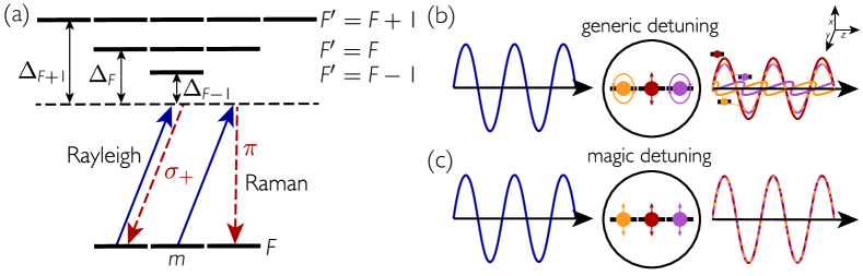
Figure 1: Scattering from a $D_{2}$-line. (a) Atoms are initiated in a hyperfine manifold $F$ and driven (blue) off-resonantly on the $D_{2}$ line with $F^{\prime}\in\{F-1,F,F+1\}$, scattering light (red). Two types of scattering processes that can occur are depicted. The atom can Rayleigh scatter, returning to its original state, or Raman scatter, changing state during the process. (b,c) An atom in an $F=1$ state is driven by a linearly $x$-polarized field and scatters light. (b) For a generic detuning, an atom prepared in a superposition of states becomes entangled with the scattered field, as the polarization and amplitude of the field depend on the magnetic state. (c) At a magic detuning, the generated field is independent of the atomic internal state.

II Generalized polarizability tensor

We consider an atom in a hyperfine state $F$, with $2F+1$ magnetic sublevels $m_{F}\in[-F,\,F]$. In the absence of an external magnetic field, these sublevels are degenerate. The atom is driven by a monochromatic field of frequency $\omega$,

$$\hat{\mathbf{E}}(\mathbf{r})=\hat{\epsilon}\,\hat{E}_{0}^{(+)}(\mathbf{r})\,\mathrm{e}^{-i\omega t}+\mathrm{c.c},$$ (1)

where $\hat{\epsilon}$ is the polarization vector, $\hat{E}_{0}^{(+)}$ is the positive-frequency component of the field, and $\mathbf{r}$ is the position of the atom. The light frequency is close to (but detuned from) a $D_{2}$ line with hyperfine levels $F^{\prime}\in\,\{F-1,\,F,\,F+1\}$, as shown in Fig. 1. The environment is assumed to be frequency selective – e.g. a resonant optical cavity – such that scattering from the $F^{\prime}$ levels to other ground hyperfine states can be neglected.

Under weak driving, such that the induced excited state population is negligible, the response of an atom in state $\ket{F,m_{F}}$ is captured by the polarizability tensor, i.e.,

$$\alpha_{\mu\nu}(F,m_{F},\omega)=$$

$$-\sum\limits_{F^{\prime},m_{F^{\prime}}}\frac{\bra{F,m_{F}}d_{\nu}\ket{F^{\prime},m_{F^{\prime}}}\bra{F^{\prime},m_{F^{\prime}}}d_{\mu}\ket{F,m_{F}}}{\hbar\Delta_{F^{\prime}}},$$ (2)

where $\mu,\nu$ are polarization indices, $d_{\nu(\mu)}$ is the atomic dipole operator projected onto polarization $\nu(\mu)$, and $\Delta_{F^{\prime}}=\omega-\omega_{F^{\prime}}$ is the detuning of the drive field from the $F-F^{\prime}$ resonance transition frequency. The above expression is derived under the rotating wave approximation, which is valid for $\Delta_{F^{\prime}}\ll\omega_{F^{\prime}}$. The polarizability tensor is normalized such that an atom in state $\ket{F,m_{F}}$ at position $\mathbf{r}$ scatters an input field to an output field at position $\mathbf{r}^{\prime}$ with polarization components

$$\hat{E}^{(+)}_{\mathrm{out}}(\mathbf{r}^{\prime})=\mu_{0}\omega^{2}\sum\limits_{\chi,\mu,\nu}G_{\chi\mu}(\mathbf{r}^{\prime},\mathbf{r},\omega)\alpha_{\mu\nu}(F,m_{F},\omega)E^{(+)}_{\nu}(\mathbf{r}).$$ (3)

In the above equation, $G_{\chi\mu}(\mathbf{r}^{\prime},\mathbf{r},\omega)$ is the Green’s tensor of the electromagnetic environment evaluated at the atomic position.

This standard form of the polarizability tensor does not describe all possible scattering processes, as it does not allow for the atom to change internal state. This can be justified by assuming scattering only due to stimulated emission by the drive and that there is a large Zeeman splitting making such Raman transitions strongly off resonant [43]. However, in the absence of a large magnetic field, one should instead consider a more general map that includes different initial and final magnetic sublevels. Inspired by Eq. (2), we define the “generalized polarizability tensor” as

$$\alpha^{nm}_{\mu\nu}(F,\omega)=$$

$$-\sum\limits_{F^{\prime},m_{F^{\prime}}}\frac{\bra{F,n}d_{\nu}\ket{F^{\prime},m_{F^{\prime}}}\bra{F^{\prime},m_{F^{\prime}}}d_{\mu}\ket{F,m}}{\hbar\Delta_{F^{\prime}}},$$ (4)

where we have dropped the subscript $F$ from the ground atomic states, simply using $m$ for the sake of clarity.

In general, the state of the atom becomes correlated with the field, and the positive-frequency component of the field operator is related to the atomic coherence operators between Zeeman sublevels as

$$\hat{\mathbf{E}}^{(+)}_{\mathrm{out}}(\mathbf{r}^{\prime})=\mu_{0}\omega^{2}\sum\limits_{\chi,\nu,\mu,m,n}G_{\chi\mu} (\mathbf{r}^{\prime},\mathbf{r},\omega)\,\alpha^{nm}_{\mu\nu}(F,\omega)$$

$$\times\hat{E}^{(+)}_{\nu}(\mathbf{r})\ket{F,m}\bra{F,n}.$$ (5)

Elements of the generalized polarizability tensor that are diagonal in the atomic state (i.e., $n=m$), correspond to Rayleigh scattering processes and are simply given by the polarizability tensor of Eq. (2). Off-diagonal elements (i.e., $n\neq m$) correspond to Raman processes. Both these processes can lead to correlations between the atom and scattered field, and so (even in the absence of Raman processes), an atom initially in a superposition of $m$ states will decohere as correlations develop. For the field to be independent of $\ket{m}\bra{n}$, we require the generalized polarizability tensor to be of the form

$$\sum\limits_{m,n}\alpha^{nm}_{\mu\nu}(F,\omega)\ket{m}\bra{n}=\alpha_{\mu\nu}(F,\omega)\,\mathbb{1},$$ (6)

i.e., for $\alpha^{nm}_{\mu\nu}$ to be diagonal in the magnetic state (this is, only non-zero when $n=m$), and $\alpha^{mm}_{\mu\nu}$ to be independent of $m$ such that the above sum over the atomic states becomes the identity. In the following, we use these criteria to find conditions on the dipole matrix elements, and find detunings at which the atomic state does not become correlated with the field.

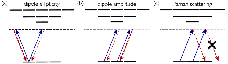
Figure 2: Scattering processes that depend on the internal atomic state. (a) The ellipticity of the field may not be preserved in the induced dipole. Due to symmetry, states $m$ and $-m$ will respond in opposite ways, and thus this process is $m$ dependent. (b) The amplitude of the induced dipole may be different for different states. (c) Scattering processes that change the magnetic state can occur. Since not all states can undergo these processes, they are $m$ dependent.

II.1 Choice of polarization basis

The coordinate system can be arbitrarily chosen without loss of generality, and so we choose both the quantization axis of the atoms and the propagation direction of the drive to be $z$. Therefore, the polarization vector of the drive field lies in the $x$-$y$ plane . Within this plane, it is convenient to work in a basis defined by the circular polarization unit vectors $\hat{\epsilon}_{\pm}=(\hat{\epsilon}_{x}\pm{\rm i}\hat{\epsilon}_{y})/\sqrt{2}$. Using this convention, we define a unit polarization vector parallel to that of the incoming light, and one perpendicular, of the form

$$\hat{\epsilon}_{\parallel}=\hat{\epsilon}_{+}\cos\theta+\hat{\epsilon}_{-}\sin\theta,~{}~{}~{}~{}\hat{\epsilon}_{\perp}=\hat{\epsilon}_{+}\sin\theta\\ -\hat{\epsilon}_{-}\cos\theta.$$ (7)

The angle $\theta$ encodes the “ellipticity” of the drive: for $\theta=\{0,\pi/2\}$, the field is purely circular, for $\theta=\pi/4$, the field is purely linear. This choice of basis requires setting the $x-y$ axes such that

$$\hat{\epsilon}_{\parallel}=\hat{\epsilon}_{x}(\cos\theta+\sin\theta)/\sqrt{2}+{\rm i}\hat{\epsilon}_{y}(\cos\theta-\sin\theta)/\sqrt{2},$$ (8)

which is to say that the $x$-axis is defined to be identical to the real part of the input light polarization vector.

II.2 Evaluating dipole matrix elements

Due to selection rules, only three sets of dipole matrix elements can be non-zero: those corresponding to $\sigma_{\pm}$- and $\pi$-polarized transitions. We define the dipole matrix elements as [see Appendix A for full expressions]

$$r_{m,F,F^{\prime}} =\bra{F,m}d_{+}\ket{F^{\prime},m+1},$$ (9a)

$$s_{m,F,F^{\prime}} =\bra{F,m}d_{-}\ket{F^{\prime},m-1},$$ (9b)

$$t_{m,F,F^{\prime}} =\bra{F,m}d_{\pi}\ket{F^{\prime},m}.$$ (9c)

These selections rules can be used to eliminate the sums over $m_{F^{\prime}}$ in the generalized polarizability tensor.

III Conditions for state independent scattering

Here, we find conditions where the scattering response of the atom is independent of the atomic state. For the generalized polarizability tensor not to correlate the output light with the atomic state, it needs to be independent of the input and output atomic state. This requires Rayleigh scattering from all states to occur at the same amplitude, and for all states not to be able to Raman scatter.

III.1 Rayleigh scattering

The first criteria we require is that the atom Rayleigh-scatters (i.e., $m=n$) at a rate that is independent of the atomic state. For scattering into the parallel mode, we need $\alpha^{mm}_{\parallel\parallel}(F,\omega)=\alpha_{\parallel\parallel}(F,\omega)~{}\forall~{}m$. These terms are given by

$$\alpha {}^{mm}_{\parallel\parallel}(F,\omega)=$$

$$-\sum\limits_{F^{\prime},m_{F^{\prime}}}\frac{\bra{F,m}d_{\parallel}\ket{F^{\prime},m_{F^{\prime}}}\bra{F^{\prime},m_{F^{\prime}}}d_{\parallel}\ket{F,m}}{\hbar\Delta_{F^{\prime}}}.$$ (10)

Since $\hat{\epsilon}_{\parallel}=\cos\theta\,\hat{\epsilon}_{+}+\sin\theta\,\hat{\epsilon}_{-}$, the above equation can be written in terms of the dipole matrix elements as

$$\alpha^{mm}_{\parallel\parallel} =-\sum\limits_{F^{\prime}}\frac{r^{2}_{m,F,F^{\prime}}+s^{2}_{m,F,F^{\prime}}}{\hbar\Delta_{F^{\prime}}}$$

$$\;\;\;\;-\sum\limits_{F^{\prime}}\frac{(\cos^{2}\theta-\sin^{2}\theta)\left(r^{2}_{m,F,F^{\prime}}-s^{2}_{m,F,F^{\prime}}\right)}{\hbar\Delta_{F^{\prime}}}.$$ (11)

For linear polarization, $\cos\theta=\sin\theta$, and for the above expression to be state independent there is only one condition: that the sum of the two different-handed terms is independent of $m$. This condition enforces that the amplitude of the induced dipole must be the same for all states.

For arbitrary elliptical polarization, the difference between the two terms must also be independent of $m$. The dipole matrix elements have the symmetry

$$r^{2}_{m,F,F^{\prime}}=s^{2}_{-m,F,F^{\prime}}.$$ (12)

Therefore, the difference between the two different-handed terms is zero for the $m=0$ state. This means that for this difference to be independent of $m$, it must be zero for all $m$. This condition enforces that the induced dipole preserves the ellipticity of the input field.

We also require that Rayleigh scattering into the perpendicular mode occurs at the same rate for all $m$. These elements can be written as

$$\alpha^{mm}_{\perp\parallel}(F,\omega)=-\sum\limits_{F^{\prime}}\frac{\bra{F,m}d_{\perp}\ket{F^{\prime},m_{F^{\prime}}}\bra{F^{\prime},m_{F^{\prime}}}d_{\parallel}\ket{F,m}}{\hbar\Delta_{F^{\prime}}}.$$ (13)

Note that $\alpha^{mm}_{\pi\parallel}=0\,\,\forall\,m$ because the atomic state must change to conserve spin when scattering $\pi$-polarized light. As above, this expression can be written in terms of dipole matrix elements as

$$\alpha^{mm}_{\perp\parallel}(F,\omega)=-\sin\theta\cos\theta\sum\limits_{F^{\prime}}\frac{\left(r_{m,F,F^{\prime}}^{2}-s_{m,F,F^{\prime}}^{2}\right)}{\hbar\Delta_{F^{\prime}}}.$$ (14)

For pure circularly-polarized input light ($\theta=\{0,\pi/2\}$) this condition is trivially met, as the above equation describes the difference in ellipticity of the input field and the induced dipole, and light with a given circular polarization cannot induce a dipole of opposite handedness. For input light with arbitrary polarization, the condition is akin to that above: the difference between the two different-handed terms must be zero for all $m$.

III.2 Raman scattering

The internal state should not change in the scattering process. Not all states can Raman scatter both polarizations of light, as shown in Fig. 2(c), and so the only possible way to eliminate $m$ dependence from the Raman scattering is for it to be zero. This means we require

$$\alpha^{nm}_{\mu\parallel}=-\sum\limits_{F^{\prime}}\frac{\bra{F,n}d_{\mu}\ket{F^{\prime},m_{F^{\prime}}}\bra{F^{\prime},m_{F^{\prime}}}d_{\parallel}\ket{F,m}}{\hbar\Delta_{F^{\prime}}}=0$$ (15)

for all $n\neq m$ and all output polarizations. Due to selection rules, only two types of Raman processes can occur, with associated polarizabilities

$$\alpha^{m+2,m}_{-+} =-\sum\limits_{F^{\prime}}\frac{r_{m,F,F^{\prime}}s_{m+2,F,F^{\prime}}}{\hbar\Delta_{F^{\prime}}},$$ (16a)

$$\alpha^{m+1,m}_{\pi+} =-\sum\limits_{F^{\prime}}\frac{r_{m,F,F^{\prime}}t_{m+1,F,F^{\prime}}}{\hbar\Delta_{F^{\prime}}}.$$ (16b)

Exploiting the generalized polarizability tensor symmetry

$$\alpha^{-n,-m}_{\nu\mp}=\alpha^{n,m}_{\mu\pm},$$ (17)

it is easy to see that processes that decrease the magnetic number are also zero when the two conditions above are met.

III.3 Summary

In summary, three conditions on the dipole matrix elements need to be satisfied for state-independent light-scattering. If they are all met at the same drive frequency for all $m$, then the generalized polarizability tensor is independent of the magnetic state and the field will not be correlated with the atomic state. The conditions are summarized below:

1. Preserved dipole ellipticity. The difference between the different-handed dipole matrix elements must be zero. This implies

   $$\sum\limits_{F^{\prime}}\frac{r^{2}_{m,F,F^{\prime}}-s^{2}_{m,F,F^{\prime}}}{\Delta_{F^{\prime}}}=0.$$ (18)

   This condition means that the induced dipole has no component perpendicular to the input field. We thus define the detuning at which this condition is met as $\Delta_{\perp}$.

2. Equal dipole amplitude. The sum of the different-handed dipole matrix elements must be independent of $m$

   $$\sum\limits_{F^{\prime}}\frac{r^{2}_{m,F,F^{\prime}}+s^{2}_{m,F,F^{\prime}}}{\Delta_{F^{\prime}}}=f(F,F^{\prime}).$$ (19)

   Meeting this condition means that the parallel component of the induced dipole has the same amplitude for all states. We thus define the detuning at which it is met as $\Delta_{\parallel}$.

3. Zero Raman scattering. Raman processes must not occur. This is guaranteed if:

   $$\sum\limits_{F^{\prime}}\frac{r_{m,F,F^{\prime}}s_{m+2,F,F^{\prime}}}{\Delta_{F^{\prime}}}=0,$$ (20a)

   $$\sum\limits_{F^{\prime}}\frac{r_{m,F,F^{\prime}}t_{m+1,F,F^{\prime}}}{\Delta_{F^{\prime}}}=0.$$ (20b)

   We define the detunings that satisfy these equations as $\Delta_{c,\pi}$ respectively.

In the following sections, we find detunings that separately satisfy each of these conditions.

IV Detunings to meet state-indepedent scattering conditions

IV.1 Preserved dipole ellipticity

Here, we find the detuning that satisfies Eq. (18). This ensures that the induced dipole has the same polarization as the input field. The sum has three terms, since $F^{\prime}\in\{F-1,F,F+1\}$ for the $D_{2}$ line. The set of three detunings $\{\Delta_{F^{\prime}}\}$ are not independent from each other, and two of them can be defined as differences from the other. We define this detuning from the central $F^{\prime}=F$ line, i.e., $\Delta_{F}\equiv\Delta$, such that $\Delta_{F\pm 1}=\Delta+\zeta_{\pm 1}$, where $\zeta_{\pm 1}=\omega_{F}-\omega_{F\pm 1}$ is the hyperfine splitting. By direct evaluation of the dipole matrix elements, the above sum becomes (see Appendix B for details)

$$\sum_{l=-1}^{1}(-1)^{l}\frac{(2+l(2F+1)-l^{2})(2F+1)-2l}{\Delta_{\perp}+|l|\,\zeta_{l}}{\{\!\{}F+l{\}\!\}}=0,$$ (21)

where ${\{\!\{}F+l{\}\!\}}$ denotes the square of a Wigner 6-j symbol of the form

$${\{\!\{}F+l{\}\!\}}\equiv\begin{Bmatrix}J&J^{\prime}&1\\ F+l&F&I\end{Bmatrix}^{2},$$ (22)

where $J$ and $J^{\prime}$ are the electron angular momentum quantum numbers of the ground and excited states respectively and $I$ is the nuclear angular momentum quantum number. Importantly, Eq. (21) contains no $m$ dependence, and so $\Delta_{\perp}$ is the same for all $m$ states. This occurs because $r^{2}_{m,F,F^{\prime}}-s^{2}_{m,F,F^{\prime}}$ is always linear in $m$, and so it simply factors out. The above equation has two trivial solutions, $\Delta_{\perp}\rightarrow\pm\infty$. These solutions simply describe that if the probe light is infinitely far detuned then all $m$ states have no response, trivially making them respond in the same way. There are also two non-trivial solutions that can be found by rearranging the expression into a quadratic equation in $\Delta_{\perp}$. There are always guaranteed to be two real non-trivial solutions for scattering on the $D_{2}$ line. Details on the form of the solutions and their derivation are provided in Appendix B.

IV.2 Equal dipole amplitude

Here we find the detuning which satisfies Eq. (19). This ensures that the induced dipole parallel to the input field has the same amplitude for all $m$ states. Following the same procedure as above, we expand the sum as three terms with $F^{\prime}\in\{F-1,F,F+1\}$ and then expand the dipole matrix elements. In this case we find that $r^{2}_{m,F,F^{\prime}}+s^{2}_{m,F,F^{\prime}}$ has two contributions: a scalar term and a term that is quadratic in $m$. For the scattering rate to be $m$ independent we thus require that the sum over the terms quadratic in $m$ is zero. As above, since the $m$ dependence is the same for every term, it simply factors out, and any solution that is found works for all $m$ states. The detuning at which the above condition is met for all $m$ states is thus the solution to

$$\sum_{l=-1}^{1}(-1)^{l}\frac{(2-l^{2})(2F+1)-l}{\Delta_{\parallel}+|l|\zeta_{l}}{\{\!\{}F+l{\}\!\}}=0.$$ (23)

This equation again has two trivial solutions, $\Delta_{\parallel}\rightarrow\pm\infty$. To find potential non-trivial solutions, we again rearrange the terms into a quadratic equation. In this case, the coefficient on the $\Delta_{\parallel}^{2}$ term is zero for the $D_{2}$ line, and thus the condition has only one non-trivial solution. Details on the form of the solution and its derivation are provided in Appendix C.

IV.3 Zero Raman scattering

IV.3.1 Circular scattering

Here, we find a detuning that satisfies Eq. (20a). Substituting in expressions for the dipole matrix elements (see Appendix A) reduces the expression to Eq. (23), and so Raman processes involving two circular photons are zero at $\Delta_{\parallel}$.

IV.3.2 $\pi$ scattering

Here, we find a detuning that satisfies Eq. (20b). By substituting in expressions for the dipole matrix elements as before we arrive at the condition

$$\sum\limits_{l=-1}^{1}(-1)^{l}\frac{(2F+1)(2m+2)+l(F(2F+2)-m-1)-l^{2}(2F+1)(m+1)}{\Delta_{\pi}+|l|\,\zeta_{l}}{\{\!\{}F+l{\}\!\}}=0.$$ (24)

Once again, the $m$-dependence takes a familiar form: we require Eq. (23) to be fulfilled. The Raman rate becomes $m$ independent at $\Delta_{\parallel}$. The $m$ independent part is zero at a third detuning condition $\Delta_{\pi}$. The expression for $\Delta_{\pi}$ can be simplified using the zero combination of the three Wigner 6-j symbols we found in the derivation of $\Delta_{\parallel}$ [Eq. (54) in App. C]. For scattering on the $D_{2}$ line it is given as

$$\Delta_{\pi}=\frac{\zeta_{+1}{\{\!\{}F{\}\!\}}}{{\{\!\{}F+1{\}\!\}}-{\{\!\{}F{\}\!\}}}.$$ (25)

V Approximating the hyperfine splitting 

The hyperfine splitting can be expressed in terms of a sum over different nuclear multipole moments [45, 46]. Typically, the largest contribution is given by the magnetic dipole moment interaction, quantified by the magnetic dipole hyperfine constant $A_{\mathrm{hfs}}$, with the largest corrections arising from the electric quadrupole and magnetic octopole moments, quantified by $B_{\mathrm{hfs}}$ and $C_{\mathrm{hfs}}$ respectively.

If the magnetic dipole moment is the sole contributor (or by far the most dominant one), the hyperfine splitting reads

$$\delta_{\mathrm{hfs}}=\frac{A_{\mathrm{hfs}}}{2}\left[F^{\prime}(F^{\prime}+1)-I(I+1)-J(J+1)\right].$$ (26)

The hyperfine splitting in the $D_{2}$ line is thus

$$\zeta_{+1}=-A_{\mathrm{hfs}}(F+1),$$ (27a)

$$\zeta_{-1}=A_{\mathrm{hfs}}F.$$ (27b)

Substituting these values into the expressions for $\Delta_{\perp},\Delta_{\parallel}$ and $\Delta_{\pi}$ we find that all three of our detunings have a common root (full details of this derivation are provided in Appendix D). This brings us to the key finding of our paper: for atoms scattering on a $D_{2}$ line, there is a detuning where the generalized polarizability tensor does not correlate the atomic state with the field at all.

VI Optimization of the state-insensitive detuning

We have shown that, for cases where hyperfine structure results only from the nuclear magnetic moment term, the hyperfine structure interval rule guarantees that all three state-independence criteria can be met at a single detuning $\Delta$. However, this interval rule does not strictly hold when higher-order nuclear moments contribute to the hyperfine structure. In this more general situation, and as shown in Table I, we no longer find a single detuning at which all three criteria apply. Nevertheless, to the extent that higher-order nuclear moments contribute only weakly to hyperfine structure, the three state-independent criteria are all approximately fulfilled at the same detuning.

Here, somewhat ad hoc, we derive a detuning at which the conditions for state-independent scattering are all nearly satisfied. We approach this problem by considering the distance between the generalized polarizability tensor from an “ideal” one, defined as $\tilde{\alpha}^{nm}_{\mu\parallel}(F,\omega)$ with entries

$$\tilde{\alpha}^{mm}_{\parallel\parallel}(F,\omega) =\alpha_{\parallel\parallel}^{00}(F,\omega)\;\forall\;m,$$ (28a)

$$\tilde{\alpha}^{nm}_{\mu\parallel}(F,\omega) =0\;\forall\;n\neq m,\mu\neq\parallel.$$ (28b)

The “magic distance” is obtained from the square of the (normalized) Frobenius norm of the difference between these two tensors, i.e.,

$$M(F,\Delta)=\sum\limits_{n,m,\mu}\left|\frac{\tilde{\alpha}^{nm}_{\mu\parallel}(F,\omega)-\alpha^{nm}_{\mu\parallel}(F,\omega)}{\alpha^{00}_{\parallel\parallel}(F,\omega)}\right|^{2}.$$ (29)

Since we use the polarization of the input field to define our basis, the only relevant parts of the generalized polarizability tensor are those with polarization parallel to the input field. As such, we only concern ourselves with the output polarization index, and initial and final atomic state indices. For species where the hyperfine spin is half-integer, there is no $m=0$ state, and the normalization is instead performed with the $m=1/2$ state. We consider that minimizing $M(F,\Delta)$ provides a “nearly state-independent scattering” detuning.

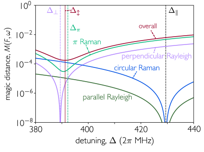
Figure 3: Optimization to find the magic detuning. The overall value of the magic distance defined by Eq. (29), is shown along with the different contributions to that value. Vertical dashed lines show the detunings that meet each condition, while the solid vertical line shows the optimized detuning. The example shown here is a ⁸⁷Rb atom in the $F=1$ line driven with linear light.

Atom	$F$	$\zeta_{+1}$ ($2\pi$ MHz)	$\zeta_{-1}$ ($2\pi$ MHz)	$B_{\mathrm{hfs}}/A_{\mathrm{hfs}}$	$\Delta_{\perp}$ ($2\pi$ MHz)	$\Delta_{\parallel}$ ($2\pi$ MHz)	$\Delta_{\pi}$ ($2\pi$ MHz)	$\Delta_{\updownarrow}$ ($2\pi$ MHz)	$M(F,\Delta_{\updownarrow})$
6Li [46]	3/2	2.9	-1.8	0.087	0.58, 2.38	2.41	2.32	2.39	$6.7\times 10^{-4}$
7Li [47]	1	6.0	-2.9	0.052	1.45, -15.0	-15.5	-15.0	-15.0	$3.0\times 10^{-5}$
7Li [47]	2	9.4	-6.0	0.052	1.55, 9.11	8.92	9.40	9.05	$9.4\times 10^{-4}$
23Na [48]	1	-34.3	15.8	0.147	-8.0, 85.1	93.8	85.8	85.5	$1.7\times 10^{-4}$
23Na [48]	2	-58.3	34.3	0.147	-9.4, -53.4	-50.3	-58.3	-52.4	$7.9\times 10^{-3}$
40K [49]	7/2	33.3	-24.2	0.45	3.5, -73.0	-77.8	-74.0	-73.4	$5.7\times 10^{-4}$
40K [49]	9/2	44.1	-33.3	0.45	3.9, 60.6	57.6	64.1	60.1	$3.0\times 10^{-3}$
85Rb [50]	2	-63.4	29.4	1.03	-7.7, 140.6	227.6	147.9	143.9	$7.2\times 10^{-3}$
85Rb [50]	3	-120.6	63.4	1.03	-13.4, -118.9	-97.3	-150.8	-113.9	$6.0\times 10^{-2}$
87Rb [51]	1	-156.9	72.2	0.148	-36.4, 389.4	429.4	392.2	391.2	$1.8\times 10^{-4}$
87Rb [51]	2	-266.7	156.9	0.148	-42.8, -244.3	-229.9	-266.7	-239.5	$8.0\times 10^{-3}$
133Cs [52]	3	-201.29	151.22	-0.00981	-25.20, 453.04	452.36	452.90	452.99	$3.0\times 10^{-7}$
133Cs [52]	4	-251.09	201.29	-0.00981	-25.12, -352.05	-352.50	-351.53	-352.13	$1.9\times 10^{-6}$

Table 1: Properties of alkali atoms, values of detunings that meet certain conditions, and optimized detunings for minimal magic distance. Only one line is presented for ⁶Li as, due to its nuclear spin $I=1$, scattering from the $F=1/2$ level is only via two $F^{\prime}$ levels. Two isotopes of potassium, ³⁹K and ⁴¹K, are also omitted, as the hyperfine structure of the $D_{2}$ line is close to degenerate and not known to sufficient accuracy to perform these calculations [49, 50].

The dependence of the magic distance with frequency, for ⁸⁷Rb, is shown in Fig. 3. Imperfections in the generalized polarizability tensor due to Rayleigh scattering into the perpendicular and parallel mode are minimized at $\Delta_{\perp}$ and $\Delta_{\parallel}$, respectively. Raman scattering of circular light is also minimized at $\Delta_{\parallel}$, while Raman scattering of $\pi$-polarized light is minimized close to $\Delta_{\pi}$. Note that this does not occur exactly at $\Delta_{\pi}$ because that detuning is only where the state-independent fraction of the Raman scattering is zero, as the $m$ dependent part is minimized at $\Delta_{\parallel}$, and so minimizing $\pi$-polarized Raman scattering is a compromise between these two values. This is also the reason why the primary contribution of imperfections to the generalized polarizability tensor is $\pi$-polarized Raman scattering. As such, the overall optimal detuning for this species lies relatively close to $\Delta_{\pi}$. Nevertheless, the magic distance is relatively flat across a fairly broad range of detunings, such that small perturbations from the optimal detuning would not drastically increase the magic distance.

VII Optimized detuning

In this Section, we calculate the relevant detunings for different species of atoms and atomic ions. We focus on alkali atoms and singly-ionized alkaline-earth atoms. In both cases, the single outer electron provides a simple and clean spectrum, and the values of $J$ and $J^{\prime}$ are always such that the above analysis is valid. We optimize for linear polarization, yielding an optimized detuning we define as $\Delta_{\updownarrow}$. It should be noted that the optimized detuning does depend on the input field, but the impact is small. The optimized detuning for circular input field is generally within 1 MHz of $\Delta_{\updownarrow}$, and for elliptical polarizations the optimal detuning varies smoothly between these values.

VII.1 Alkali atoms

We first consider alkali atoms. These encompass species with both integer and half-integer hyperfine spin, as well as a variety of nuclear spin. Table 1 shows the detuning conditions $\Delta_{\perp,\parallel,\pi}$ for experimentally relevant alkalis, as well as the optimized detuning $\Delta_{\updownarrow}$ and the magic distance at that detuning.

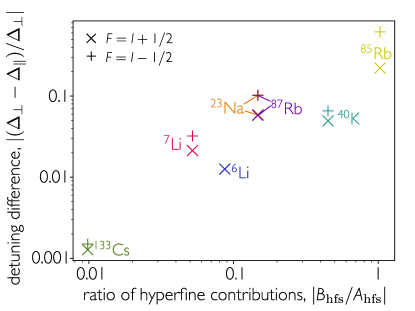
Figure 4: The normalized difference between $\Delta_{\perp}$ and $\Delta_{\parallel}$, as a function of the ratio of (electric quadrupole vs magnetic dipole) hyperfine contributions, $|B_{\mathrm{hfs}}/A_{\mathrm{hfs}}|$. $\Delta_{\perp}$ is chosen as the solution closest to $\Delta_{\parallel}$. Generically, when the relative contribution of the electric quadrupole moment is very small then the two detunings are closer to one another. Data is shown for ground state hyperfine manifolds $F=I+1/2$ (+ symbols) and $F=I-1/2$ ($\times$ symbols).

.

Ion	$F$	$\zeta_{+1}$ ($2\pi$ MHz)	$\zeta_{-1}$ ($2\pi$ MHz)	$B_{\mathrm{hfs}}/A_{\mathrm{hfs}}$	$\Delta_{\perp}$ ($2\pi$ MHz)	$\Delta_{\parallel}$ ($2\pi$ MHz)	$\Delta_{\pi}$ ($2\pi$ MHz)	$\Delta_{\updownarrow}$ ($2\pi$ MHz)	$M(F,\Delta_{\updownarrow})$
43Ca+ [53]	3	122.0	-88.1	0.223	14.8, -272.6	-282.3	-274.5	-273.3	$1.5\times 10^{-4}$
43Ca+ [53]	4	159.9	-122.0	0.223	15.8, 216.4	210.3	223.9	215.4	$1.0\times 10^{-3}$
85Sr+ [54]	4	275.0	-315.9	-4.08	36.3, -657.8	-503.2	-605.0	-642.2	$0.023$
85Sr+ [54]	5	154.1	-275.0	-4.08	15.0, 423.5	846.3	213.2	450.2	$0.199$
87Sr+ [54]	4	198.4	-203.0	-2.46	24.0, -461.0	-381.1	-436.5	-453.4	$0.010$
87Sr+ [54]	5	157.0	-198.4	-2.46	14.4, 323.8	439.7	235.5	336.1	0.069
89Sr+ [54]	2	171.9	-77.9	1.07	20.5, -380.2	-643.7	-401.1	-389.7	$8.0\times 10^{-3}$
89Sr+ [54]	3	331.9	-171.9	1.07	36.6, 324.4	263.2	414.9	310.2	0.065
91Sr+ [54]	2	163.3	-115.0	-0.234	28.5, -384.5	-365.4	-381.0	-383.0	$2.1\times 10^{-4}$
91Sr+ [54]	3	200.6	-163.3	-0.234	27.5, 273.2	271.2	275.8	272.8	$7.4\times 10^{-5}$
135Ba+ [55]	1	-167.0	54.0	0.522	-27.9, 403.7	920.2	417.5	413.0	$3.8\times 10^{-3}$
135Ba+ [55]	2	-398.0	167.0	0.522	-56.3, -294.9	-233.2	-398.0	-272.6	0.118
137Ba+ [55]	1	-161.9	34.7	0.727	-18.4, 382.6	-1216.0	404.8	398.4	0.011
137Ba+ [55]	2	-474.1	161.9	0.727	-60.9, -314.9	-221.3	-474.1	-283.9	0.251
221Ra+ [56]	2	681.1	-1136.2	-60.9	231.9, -1946.4	-1073.6	-1589.2	-1833.0	0.084
221Ra+ [56]	3	-1001.8	-681.1	-60.9	-227.8, 623.9	734.9	-1252.3	N/A	N/A
223Ra+ [56]	1	751.8	-808.3	15.3	368.7, -2060.2	-1224.5	-1879.5	-1965.4	0.025
223Ra+ [56]	2	-1034.3	-751.8	15.3	-270.0, 720.6	795.2	-1034.3	N/A	N/A

Table 2: Properties of singly-ionized alkaline earth ions and values of detunings that meet certain conditions, and optimized detunings for minimal magic distance. All integer hyperfine spin isotopes of alkaline-earth atoms have no nuclear spin, and therefore no hyperfine splitting, while ¹³³Ba⁺ cannot have a magic detuning due to its nuclear spin of $I=1/2$. For the higher $F$ level for both radium isotopes, the optimization procedure for linear polarization finds no minima between $\Delta_{\perp}$ and $\Delta_{\pi}$, such that it instead finds the trivial $\Delta\rightarrow\infty$ solutions, and so no optimized detuning is obtained.

The detuning conditions share a similar root for all considered species. The most dissimilar are found for ⁸⁵Rb, where the $F=2$ line has roots almost 80 MHz apart. The closest are found for ¹³³Cs, where they are within 1 MHz of each other. As anticipated, this is directly related to the contributions to the hyperfine splitting, as ⁸⁵Rb and ¹³³Cs have the highest and lowest relative electric quadrupole contributions respectively. Figure 4 shows that, generically, the relative detuning difference decreases together with the relative electric quadrupole contribution. The two species that do not perfectly fit this trend are the two fermionic isotopes ⁶Li and ⁴⁰K, where the difference is smaller than the general trend. For these species, the different nuclear spin means the electric quadrupole shift contribution is of a different magnitude even for the same $B_{\mathrm{hfs}}$. Since ²³Na and ⁸⁷Rb have the same ratio of hyperfine contributions and the same nuclear spin, they also have the same detuning difference. For all species, the detuning difference is smaller for the hyperfine level $F=I+1/2$ than for $F=I-1/2$.

The usefulness of these magic wavelengths is likely greatly reduced for lithium experiments, as the detuning is found very close to a resonance. For ⁶Li, the detuning conditions are met less than 1 MHz from resonance with the $F^{\prime}=1/2$ excited state. For ⁷Li, they are met around 6 MHz and 10 MHz from excited state resonances for the $F=1$ and $F=2$ respectively. Therefore, to meet the criterion of essentially no atomic excitation, one would need to use extremely weak laser power. Furthermore, there will be much higher sensitivity to frequency differences between magnetic sublevels.

VII.2 Alkaline-earth ions

For singly-ionized alkaline-earth ions, the hyperfine splitting contributions are generally not dominated by the magnetic dipole moment. For many ions, the optimized detuning is thus less magic than for the majority of alkali atoms. Two exceptions are ⁴³Ca⁺ and ⁹¹Sr⁺, where the optimized detuning should provide close to magic behavior. For many ions, the electric quadrupole contribution is actually larger than the magnetic dipole contribution. This is best exemplified by the two radium isotopes, where for some choices of $F$ and input polarization, the optimization procedure instead finds the trivial $\Delta\rightarrow\infty$ solutions rather than any local minima.

VIII Applications

VIII.1 Magic wavelength for ground state Zeeman levels: state-independent ac Stark shift

The ac Stark shift on a level $\ket{F,m_{F}}$ induced by the input light is readily given by

$$\Delta E(F,m,\omega)=-\sum\limits_{\mu,\nu}\mathrm{Re}\left[\alpha^{mm}_{\mu\nu}(F,\omega)\right]E_{\mu}^{(-)}(\mathbf{r})E_{\nu}^{(+)}(\mathbf{r}).$$ (30)

Unraveling the polarizability in terms of the dipole matrix elements, the shift reduces to

$$\Delta E(F,m,\omega) =\sum\limits_{F^{\prime}}\frac{|E_{0}^{(+)}|^{2}}{\Delta_{F^{\prime}}}\left[\left(r^{2}_{m,F,F^{\prime}}+s^{2}_{m,F,F^{\prime}}\right)+\right.$$

$$\left.\left(\cos^{2}\theta-\sin^{2}\theta\right)\left(r^{2}_{m,F,F^{\prime}}-s^{2}_{m,F,F^{\prime}}\right)\right],$$ (31)

which implies that the ac Stark shift is also independent of $m$ for $\Delta_{\parallel}=\Delta_{\perp}$. As expected, the detuning that offers the closest to a magic wavelength depends on the polarization of the field.

The conditions we found above directly relate to the traditional conception of the ac Stark shift as scalar, vector, and tensor shifts. Our condition for preserved dipole ellipticity also makes the vector Stark shift zero, while the condition for equal dipole amplitudes removes the $m^{2}$ dependence of the tensor shift.

While the values for the optimized detuning we find here are too close to resonance to efficiently trap atoms without significant atomic saturation and heating, the magic detuning can be useful in other contexts. For instance, the state independent ac Stark shift is translated to state-insensitive mechanical forces, potentially allowing for optomechanical applications where the atomic internal state can be traced out. The magic detuning could then be used to explore driven-dissipative models for optomechanics in cavity QED [57, 58, 59].

VIII.2 State-independent scattering in cavity QED

One consequence of the magic detuning is the ability to perform cavity and waveguide QED experiments without the need for careful state preparation. In waveguide QED, emitters are strongly coupled to a continuum of confined propagating modes [60, 61]. Frequency selection to eliminate scattering to the other hyperfine ground state could be achieved with a photonic crystal waveguide [62]. One complication is that the confinement of the field allows for a longitudinal polarization component, such that the coordinate system considered above is incomplete. However, Rayleigh scattering of $\pi$-polarized light must also be state-independent at the magic detuning due to symmetry arguments.

State-independent scattering was harnessed in Ref. [42], where a tweezer array of atoms was placed in a cavity to observe collective photon emission. Generically, this is a complicated problem involving atoms scattering drive photons into the cavity, exchanging photons with the cavity, and changing their internal state. However, by operating at the magic detuning, one can eliminate the internal atomic state, reducing the Hamiltonian to an effective drive of the cavity and a dispersive shift to its frequency. In this experiment, scattering at the magic detuning enabled the observation of superradiant and subradiant scattering from an atomic array into the cavity, and the reduction of the Hamiltonian to that of two-level systems was confirmed by polarization measurements of the output light. A full derivation of the Hamiltonian in this limit is provided in Appendix F.

IX Conclusions

In conclusion, we have shown the generic existence of a “magic detuning” for scattering on the $D_{2}$ line of alkali atoms and alkaline-earth ions. At this detuning, a driven atom will respond in the same manner regardless of the magnetic sublevel the atom is in, to very good approximation. This means that the complex level structure of a single hyperfine level driven off-resonantly via three excited manifolds reduces to that of an off-resonantly driven two-level atom. This eliminates the need of magnetic state preparation in quantum optics and atomic physics experiments. At the magic detuning, a prepared superposition of magnetic states is not altered by the trapping light, nor does it decohere due to correlations with the scattered light.

The magic detuning strictly occurs only in the absence of dc magnetic fields. Generally, Zeeman shifts must be small in comparison to the frequency range in which the response is close to magic. The magic condition also requires scattering to be via three excited hyperfine manifolds. Therefore, the nuclear spin has to be $I\geq 1$. The requirement for three excited manifolds means that scattering on a $D_{1}$ line cannot be magic. The necessary conditions for scattering on a $D_{1}$ line can be met independently, but they do not coincide (see Appendix E for details). Moreover, we have neglected scattering to other hyperfine ground levels assuming that the environment is frequency selective (such as, for instance, a cavity). If the environment is not frequency selective, such as in free space, the lifetime of atoms would be limited by the rate of spontaneous emission to the other hyperfine level, as spontaneous emission to both hyperfine levels cannot be state-independent at the same detuning. Repopulation of the desired hyperfine level is possible through a repump field, which can be trivially magic if the hyperfine splitting between the two hyperfine levels is much larger than that between the excited levels, such that the pump is effectively infinitely detuned. However, spontaneous emission and repumping will still decohere the atomic state. This limits the usefulness of the magic detuning in free space to situations where strictly maintaining coherence between the magnetic states is not crucial.

The level to which the magic detuning conditions hold depends on the origin of the hyperfine splitting of the excited states. If the magnetic dipole dominates over the electric quadrupole (and higher order moments), the approximation is very good. While we have focused on single-valence electron atoms and ions, the same physics may hold for the multi-electron case. To find Zeeman-insensitive frequencies, one must find a combination of the quantum numbers that meets the necessary criterion given in Eq. (54) in App. C. One has to be careful with multi-valence electron atoms, where the spectrum is more cluttered and hyperfine splitting is more complicated as it must include “configuration interactions” [45, 63]. However, as evidenced by the case of ⁸⁵Rb, where the electric quadrupole contribution to the hyperfine splitting is of similar magnitude to that of the magnetic dipole, the magic detuning is very robust to other sources of hyperfine splitting. Therefore, if the hyperfine splitting is still given by the magnetic dipole contribution to even a broad approximation, the two-level picture may still be a good approximation. The presence of a magic detuning may also be interesting in the context of molecules, where magic conditions for trapping have been found for rotational states [64, 65]. However, the presence of a cluttered spectrum due to rotational and vibrational states may prove problematic.

Acknowledgments- We thank Luis Orozco and Francis Robicheaux for helpful comments. We acknowledge support from the AFOSR (Grant No. FA9550-1910328 and Young Investigator Prize Grant No. 21RT0751), from ARO through the MURI program (Grant No. W911NF-20-1-0136), from DARPA (Grant No. W911NF2010090), from the NSF (QLCI program through grant number OMA-2016245, and CAREER Award No. 2047380), and from the David and Lucile Packard Foundation. J.H. acknowledges support from the National Defense Science and Engineering Graduate (NDSEG) fellowship.

Appendix A Evaluating the dipole matrix elements 

Using the Wigner-Eckart theorem, the dipole matrix elements for the atomic transitions are given by

$$\bra{F,m}d_{\nu}\ket{F^{\prime},m_{F^{\prime}}}=\langle J||\mathbf{d}||J^{\prime}\rangle(-1)^{2F^{\prime}+m_{F}+J+I}\sqrt{(2F+1)(2J+1)(2F^{\prime}+1)}\begin{Bmatrix}J&J^{\prime}&1\\ F^{\prime}&F&I\end{Bmatrix}\begin{pmatrix}F&1&F^{\prime}\\ m&q&-m-q\end{pmatrix},$$ (32)

where $q\in\{-1,0,+1\}$ corresponds to photons with polarization $\nu\in\{\sigma_{-},\pi,\sigma_{+}\}$, respectively. It is convenient to work in units such that $\langle J||\mathbf{d}||J^{\prime}\rangle(-1)^{2F^{\prime}+J+I}\sqrt{(2F+1)(2J+1)}=1$, as this is a constant for all transitions from a given hyperfine manifold. In these units, we define dipole matrix elements as

$$r_{F,F^{\prime}}^{m} =(-1)^{m}\sqrt{2F^{\prime}+1}\begin{Bmatrix}J&J^{\prime}&1\\ F^{\prime}&F&I\end{Bmatrix}\begin{pmatrix}F&1&F^{\prime}\\ m&1&-m-1\end{pmatrix},$$ (33a)

$$s_{F,F^{\prime}}^{m} =(-1)^{m}\sqrt{2F^{\prime}+1}\begin{Bmatrix}J&J^{\prime}&1\\ F^{\prime}&F&I\end{Bmatrix}\begin{pmatrix}F&1&F^{\prime}\\ m&-1&-m+1\end{pmatrix},$$ (33b)

$$t_{F,F^{\prime}}^{m} =(-1)^{m}\sqrt{2F^{\prime}+1}\begin{Bmatrix}J&J^{\prime}&1\\ F^{\prime}&F&I\end{Bmatrix}\begin{pmatrix}F&1&F^{\prime}\\ m&0&-m\end{pmatrix},$$ (33c)

where $J$ is the total electron angular momentum quantum number, $I$ is the nuclear spin quantum number, and $\{~{}\}$ and $(~{})$ represent Wigner 6-j and 3-j symbols respectively.

A.1 Expressions for Wigner 3-j symbols

The Wigner 3-j symbols can be calculated using the Racah formula. They are given by

$$\begin{pmatrix}F&1&F^{\prime}\\ m&1&-m-1\end{pmatrix}=(-1)^{2F+m-F^{\prime}+1}\sqrt{\frac{2(F+F^{\prime}-1)!}{(F^{\prime}-F+1)!(F-F^{\prime}+1)!(F+F^{\prime}+2)!}\frac{(F-m)!(F^{\prime}+m+1)!}{(F+m)!(F^{\prime}-m-1)!}},$$ (34a)

$$\begin{pmatrix}F&1&F^{\prime}\\ m&-1&-m+1\end{pmatrix}=(-1)^{F+m}\sqrt{\frac{2(F+F^{\prime}-1)!}{(F^{\prime}-F+1)!(F-F^{\prime}+1)!(F+F^{\prime}+2)!}\frac{(F+m)!(F^{\prime}-m+1)!}{(F-m)!(F^{\prime}+m-1)!}}.$$ (34b)

For $\pi-$polarized transitions, it is necessary to write expressions for each $F^{\prime}$ separately. The Wigner 3-j symbols are

$$\begin{pmatrix}F&1&F+1\\ m&0&-m\end{pmatrix}=(-1)^{F-1+m}\sqrt{\frac{2(F+1-m)(F+1+m)}{(2F+1)(2F+2)(2F+3)}},$$ (35a)

$$\begin{pmatrix}F&1&F+1\\ m&0&-m\end{pmatrix}=(-1)^{F-1+m}\frac{2m}{\sqrt{2F(2F+1)(2F+2)},}$$ (35b)

$$\begin{pmatrix}F&1&F-1\\ m&0&-m\end{pmatrix}=(-1)^{F+m}\sqrt{\frac{2(F+m)(F-m)}{(2F-1)2F(2F+1)}}.$$ (35c)

A.2 Expressions for Wigner 6-j symbols

Similarly, the Wigner 6-j symbols can also be calculated by the Racah formula. For the $D_{1}$ and $D_{2}$ lines respectively, they are given as

$$\begin{Bmatrix}\frac{1}{2}&\frac{1}{2}&1\\ F^{\prime}&F&I\end{Bmatrix} =\left(-1\right)^{F^{\prime}+F+1}\sqrt{\frac{\left(F^{\prime}-F+1\right)!\left(F-F^{\prime}+1\right)!\left(F^{\prime}+F+2\right)\left(F^{\prime}+F+1\right)\left(F^{\prime}+F\right)}{6\left(F+I+\frac{3}{2}\right)\left(F+I+\frac{1}{2}\right)\left(F^{\prime}+I+\frac{3}{2}\right)\left(F^{\prime}+I+\frac{1}{2}\right)}}$$ (36a)

$$\begin{Bmatrix}\frac{1}{2}&\frac{3}{2}&1\\ F^{\prime}&F&I\end{Bmatrix} =\left(-1\right)^{F^{\prime}+I+3/2}\left(I+F^{\prime}+\frac{5}{2}\right)!$$

$$\times\sqrt{\frac{\left(F^{\prime}+\frac{3}{2}-I\right)!\left(I-F+\frac{3}{2}\right)!\left(F^{\prime}+F-1\right)!}{12\left(I+F+\frac{3}{2}\right)\left(I+F+\frac{1}{2}\right)\left(F^{\prime}+I-\frac{3}{2}\right)!\left(F^{\prime}-F+1\right)!\left(F-F^{\prime}+1\right)!\left(F+I+\frac{5}{2}\right)!\left(F^{\prime}+F+2\right)!}}$$ (36b)

Appendix B Derivation of $\Delta_{\perp}$

In Sec. IV.1, we find a solution to

$$\sum\limits_{F^{\prime}}\frac{r^{2}_{m,F,F^{\prime}}-s^{2}_{m,F,F^{\prime}}}{\Delta_{F^{\prime}}}=0.$$ (37)

Using the analytic expressions for the dipole matrix elements (see Appendix A), this condition becomes

$$\sum\limits_{F^{\prime}}\frac{(2F^{\prime}+1)\begin{Bmatrix}J&J^{\prime}&1\\ F^{\prime}&F&I\end{Bmatrix}^{2}}{\Delta_{F^{\prime}}}\left[\begin{pmatrix}F&1&F^{\prime}\\ m&1&-m-1\end{pmatrix}^{2}-\begin{pmatrix}F&1&F^{\prime}\\ m&-1&-m+1\end{pmatrix}^{2}\right]=0.$$ (38)

We can then evaluate the Wigner 3-j symbols (see Appendix A.1 for expressions) to find

$$\sum\limits_{F^{\prime}}\frac{1}{\Delta_{F^{\prime}}}\frac{2(2F^{\prime}+1)(F+F^{\prime}-1)!\begin{Bmatrix}J&J^{\prime}&1\\ F^{\prime}&F&I\end{Bmatrix}^{2}}{(F^{\prime}-F+1)!(F-F^{\prime}+1)!(F+F^{\prime}+2)!}\left[\frac{(F-m)!(F^{\prime}+m+1)!}{(F+m)!(F^{\prime}-m-1)!}-\frac{(F+m)!(F^{\prime}-m+1)!}{(F-m)!(F^{\prime}+m-1)!}\right]=0.$$ (39)

For all possible values of $F^{\prime}\in\{F-1,F,F+1\}$ the expression in the square brackets is always linear in $m$, such that all $m$ dependence can be eliminated. The solution to Eq. (37) is thus $m$ independent.

As in the main text, we denote the detuning at which induced ellipticity goes to zero as $\Delta_{\perp}$. We focus on the $D_{2}$ line, so we define this detuning from the central excited line $F^{\prime}=F$, such that we make the substitutions $\Delta_{F}=\Delta_{\perp}$ and $\Delta_{F\pm 1}=\Delta_{\perp}+\zeta_{\pm 1}$. Our condition then becomes

$$\frac{2F(2F+3)}{\Delta_{\perp}+\zeta_{+1}}\begin{Bmatrix}J&J^{\prime}&1\\ F+1&F&I\end{Bmatrix}^{2}-\frac{4F+2}{\Delta_{\perp}}\begin{Bmatrix}J&J^{\prime}&1\\ F&F&I\end{Bmatrix}^{2}+\frac{(1-2F)(2F+2)}{\Delta_{\perp}+\zeta_{-1}}\begin{Bmatrix}J&J^{\prime}&1\\ F-1&F&I\end{Bmatrix}^{2}=0.$$ (40)

This can be rearranged into a quadratic equation in the detuning. It has two solutions of the form

$$\Delta_{\perp}=\frac{-b\pm\sqrt{b^{2}-4ac}}{2a},$$ (41)

where

$$a =2F(2F+3)\begin{Bmatrix}J&J^{\prime}&1\\ F+1&F&I\end{Bmatrix}^{2}-(4F+2)\begin{Bmatrix}J&J^{\prime}&1\\ F&F&I\end{Bmatrix}^{2}+(1-2F)(2F+2)\begin{Bmatrix}J&J^{\prime}&1\\ F-1&F&I\end{Bmatrix}^{2},$$ (42a)

$$b =\zeta_{-1}2F(2F+3)\begin{Bmatrix}J&J^{\prime}&1\\ F+1&F&I\end{Bmatrix}^{2}-(\zeta_{-1}+\zeta_{+1})(4F+2)\begin{Bmatrix}J&J^{\prime}&1\\ F&F&I\end{Bmatrix}^{2}+\zeta_{+1}(1-2F)(2F+2)\begin{Bmatrix}J&J^{\prime}&1\\ F-1&F&I\end{Bmatrix}^{2},$$ (42b)

$$c =-(4F+2)\begin{Bmatrix}J&J^{\prime}&1\\ F&F&I\end{Bmatrix}^{2}\zeta_{-1}\zeta_{+1}.$$ (42c)

This is guaranteed to yield two solutions because $a\neq 0$ and $b^{2}-4ac>0$ for $F\geq 1$, which is required to scatter off the $D_{2}$ line, as shown below.

B.1 Proof that there are always two roots to the equation for $\Delta_{\perp}$ for scattering on the $D_{2}$ line 

Here we demonstrate the presence of two values of $\Delta_{\perp}$ that solve Eq. (40) for the cases of $J=1/2$ and $J^{\prime}=3/2$. We define

$$A =2F(2F+3)\begin{Bmatrix}\frac{1}{2}&\frac{3}{2}&1\\ F+1&F&I\end{Bmatrix}^{2},$$ (43a)

$$B =-(4F+2)\begin{Bmatrix}\frac{1}{2}&\frac{3}{2}&1\\ F&F&I\end{Bmatrix}^{2},$$ (43b)

$$C =(1-2F)(2F+2)\begin{Bmatrix}\frac{1}{2}&\frac{3}{2}&1\\ F-1&F&I\end{Bmatrix}^{2},$$ (43c)

such that the coefficients of the quadratic equation read

$$a=A+B+C,\;\;\;\;\;\;b=\zeta_{-1}A+(\zeta_{-1}+\zeta_{+1})B+\zeta_{+1}C,\;\;\;\;\;\;c=\zeta_{-1}\zeta_{+1}B.$$ (44)

For there to be two physical roots we require $a\neq 0$ and $b^{2}-4ac>0$. For the cases where $J=1/2$ and $J^{\prime}=3/2$, we can use the identity

$$\frac{F^{2}(F+J-I+2)(F+J+I+3)}{(J+I-F+1)(F+I-J)(2F+3)}-2F-1+\frac{(F+1)^{2}(J+I-F+2)(F+I-J-1)}{(F+J-I+1)(2F-1)(F+J+I+2)}=0$$ (45)

which will be proven in Appendix C.1. We then simplify the expression such that the condition for $a=0$ is

$$\begin{Bmatrix}\frac{1}{2}&\frac{3}{2}&1\\ F+1&F&I\end{Bmatrix}^{2}=\begin{Bmatrix}\frac{1}{2}&\frac{3}{2}&1\\ F&F&I\end{Bmatrix}^{2}.$$ (46)

This cannot be true for any combination of $F$ and $I$ that satisfy $F=I\pm J$ and $F\geq 1$, and so there are always two roots to the quadratic equation. For those roots to be real we require

$$(A\zeta_{-1}+B(\zeta_{-1}+\zeta_{+1})+C\zeta_{+1})^{2}>4(A+B+C)(B\zeta_{-1}\zeta_{+1}).$$ (47)

Expanding out allows for the rearrangement

$$A^{2}\zeta_{-1}^{2}+2AC\zeta_{-1}\zeta_{+1}+B^{2}(\zeta_{-1}-\zeta_{+1})^{2}+C^{2}\zeta_{+1}^{2}>2AB\zeta_{-1}(\zeta_{+1}-\zeta_{-1})+2BC\zeta_{+1}(\zeta_{-1}-\zeta_{+1}).$$ (48)

We can use the expressions above to see that $A$ is positive, $B$ is negative, and $C$ is negative for $F\geq 1$ which is required for scattering on the $D_{2}$ line. Furthermore, $\zeta_{\pm 1}$ have opposite signs. This means that all terms on the left-hand side are positive, while only one of the terms on the right-hand side can be, depending on the sign of $\zeta_{+1}-\zeta_{-1}$. We can bound the size of these terms through (the same process can be followed if $2BC\zeta_{+1}(\zeta_{-1}-\zeta_{+1})$ is positive)

$$\left(A\zeta_{-1}-B\left(\zeta_{+1}-\zeta_{-1}\right)\right)^{2}\geq 0\Rightarrow A^{2}\zeta_{-1}+B^{2}\left(\zeta_{+1}-\zeta_{-1}\right)^{2}\geq 2AB\zeta_{-1}(\zeta_{+1}-\zeta_{-1}),$$ (49)

and show that the inequality is always valid, and Eq. (40) always has two real non-trivial roots.

Appendix C Derivation of $\Delta_{\parallel}$

In Sec. IV.2, we find a detuning where

$$S_{m,F,F^{\prime}}(\omega)=\sum\limits_{F^{\prime}}\frac{r^{2}_{m,F,F^{\prime}}+s^{2}_{m,F,F^{\prime}}}{\Delta_{F^{\prime}}}$$ (50)

is independent of $m$. By substituting in expressions for the dipole matrix elements and Wigner 3-j symbols (see Appendix A) we find

$$S_{m,F,F^{\prime}}(\omega)=\sum\limits_{F^{\prime}}\frac{1}{\Delta_{F^{\prime}}}\frac{2(2F^{\prime}+1)(F+F^{\prime}-1)!\begin{Bmatrix}J&J^{\prime}&1\\ F^{\prime}&F&I\end{Bmatrix}^{2}}{(F^{\prime}-F+1)!(F-F^{\prime}+1)!(F+F^{\prime}+2)!}\left[\frac{(F-m)!(F^{\prime}+m+1)!}{(F+m)!(F^{\prime}-m-1)!}+\frac{(F+m)!(F^{\prime}-m+1)!}{(F-m)!(F^{\prime}+m-1)!}\right].$$ (51)

This can be simplified to

$$S_{m,F,F^{\prime}}(\omega)=\left[\frac{F^{2}+3F+2+m^{2}}{(2F+1)(2F+2)}\frac{\begin{Bmatrix}J&J^{\prime}&1\\ F+1&F&I\end{Bmatrix}^{2}}{\Delta+\zeta_{+1}}+\frac{F^{2}+F-m^{2}}{F(2F+2)}\frac{\begin{Bmatrix}J&J^{\prime}&1\\ F&F&I\end{Bmatrix}^{2}}{\Delta}+\frac{F^{2}-F+m^{2}}{2F(2F+1)}\frac{\begin{Bmatrix}J&J^{\prime}&1\\ F-1&F&I\end{Bmatrix}^{2}}{\Delta+\zeta_{-1}}\right],$$ (52)

where we use the same convention above that detunings are defined from the $F^{\prime}=F$ level. For the scattering to be $m$ independent simply requires that the sum of the quadratic terms is zero. The detuning $\Delta_{\parallel}$ thus satisfies the condition

$$\frac{2F}{\Delta_{\parallel}+\zeta_{+1}}\begin{Bmatrix}J&J^{\prime}&1\\ F+1&F&I\end{Bmatrix}^{2}-\frac{4F+2}{\Delta_{\parallel}}\begin{Bmatrix}J&J^{\prime}&1\\ F&F&I\end{Bmatrix}^{2}+\frac{2F+2}{\Delta_{\parallel}+\zeta_{-1}}\begin{Bmatrix}J&J^{\prime}&1\\ F-1&F&I\end{Bmatrix}^{2}=0.$$ (53)

As above, this can be rearranged to a quadratic equation in $\Delta_{\parallel}$. However, for scattering on the $D_{2}$ line, the $\Delta_{\parallel}^{2}$ coefficient in that equation is

$$2F\begin{Bmatrix}\frac{1}{2}&\frac{3}{2}&1\\ F+1&F&I\end{Bmatrix}^{2}-(4F+2)\begin{Bmatrix}\frac{1}{2}&\frac{3}{2}&1\\ F&F&I\end{Bmatrix}^{2}+(2F+2)\begin{Bmatrix}\frac{1}{2}&\frac{3}{2}&1\\ F-1&F&I\end{Bmatrix}^{2}=0.$$ (54)

This is also true for other combinations of $J$, $J^{\prime}$ and $F$, but not all, as discussed in Appendix C.1. This means that Eq. (53) has only one solution

$$\Delta_{\parallel}=\frac{(2F+1)\begin{Bmatrix}\frac{1}{2}&\frac{3}{2}&1\\ F&F&I\end{Bmatrix}^{2}\zeta_{+1}\zeta_{-1}}{F\begin{Bmatrix}\frac{1}{2}&\frac{3}{2}&1\\ F+1&F&I\end{Bmatrix}^{2}\zeta_{-1}-(2F+1)\begin{Bmatrix}\frac{1}{2}&\frac{3}{2}&1\\ F&F&I\end{Bmatrix}^{2}(\zeta_{+1}+\zeta_{-1})+(F+1)\begin{Bmatrix}\frac{1}{2}&\frac{3}{2}&1\\ F-1&F&I\end{Bmatrix}^{2}\zeta_{+1}}.$$ (55)

C.1 Proof that there is only one root to the equation for $\Delta_{\parallel}$ for $J^{\prime}=J+1$

The quadratic coefficient for the condition to find $\Delta_{\parallel}$ is

$$D=2F\begin{Bmatrix}J&J^{\prime}&1\\ F+1&F&I\end{Bmatrix}^{2}-(4F+2)\begin{Bmatrix}J&J^{\prime}&1\\ F&F&I\end{Bmatrix}^{2}+(2F+2)\begin{Bmatrix}J&J^{\prime}&1\\ F-1&F&I\end{Bmatrix}^{2}.~{}$$ (56)

For there to be a single non-trivial root for $\Delta_{\parallel}$, and for the magic detuning to exist when the hyperfine splitting is dominated by the magnetic dipole contribution, we require $D=0$. There are three possible cases of $J^{\prime}=\{J-1,J,J+1\}$. In the following, we treat the specific case of $J^{\prime}=J+1$, a class which includes scattering on a $D_{2}$ line. In this case we have that

$$\begin{Bmatrix}J&J+1&1\\ F^{\prime}&F&I\end{Bmatrix}^{2}=g(F,I,J)\frac{(F^{\prime}+J-I+1)!(J+I-F^{\prime}+1)!(F^{\prime}+F-1)!(F^{\prime}+J+I+2)!}{(F^{\prime}+I-J-1)!(F^{\prime}-F+1)!(F-F^{\prime}+1)!(F^{\prime}+F+2)!},$$ (57)

where $g(F,I,J)$ is a function that does not depend on $F^{\prime}$ and so is a constant factor in Eq. (56). Using this expression we find that the condition for $D=0$ becomes

$$\frac{F^{2}(F+J-I+2)(F+J+I+3)}{(J+I-F+1)(F+I-J)(2F+3)}-2F-1+\frac{(F+1)^{2}(J+I-F+2)(F+I-J-1)}{(F+J-I+1)(2F-1)(F+J+I+2)}=0.$$ (58)

The ground state hyperfine level must have $F=I+J-n$ where $n\in\mathbb{N}$ is a positive integer (or zero) such that $F\geq 1$, $F\geq J-I$ and $F\geq I-J$. We can use this to simplify the expression and find solutions for a particular $n$. A few pertinent examples are given below. Cases not covered here can be found by setting $F=I+J-n$, inputting in the specific values of $I$ and $J$ and solving for $n$. If $n$ meets the criteria above then a magic detuning exists for that combination of $F$, $I$ and $J$.

C.1.1 $n=0$

For $n=0$, $F=I+J$ is the maximum angular momentum hyperfine level. Solutions are found by solving

$$F^{2}(2F-1)(2J+2)(2J+1)-(2F+1)(2F-1)(2F-2J)(2J+1)+(F+1)(2F-2J-1)(2F-2J)=0.$$ (59)

This expression has five roots which can be found by rearranging to the form

$$2F(2F^{2}+3F+1)J(2J-1)=0.$$ (60)

Three of the roots are found as $F=0,-1/2,-1$. All of these are unphysical as we require $F\geq 1$. As such, the only roots are $J=0,1/2$. This means a magic detuning exists for scattering via a line where $J^{\prime}=J+1$ for $J=0$, $F=I$, and for $J=1/2$, $F=I+1/2$. The second case is exactly that for scattering on the $D_{2}$ line from the highest $F$ hyperfine level.

C.1.2 $n=1$

For $n=1$, $F=I+J-1$ is the second highest angular momentum hyperfine level. Solutions are found by solving

$$F^{2}J(2F-1)(2J+1)(F+2)-J(2F+1)(2F-1)(2F-2J+1)(2F+3)+3(F+1)^{2}(F-J)(2F-2J+1)=0.$$ (61)

Unlike the equation above, this does not reduce to an easily solved form, but it can be shown that there are physical solutions for $J=1/2$ with $F$ free and for $F=5,J=2$. The former case is again that for the $D_{2}$ line, but now from the lower hyperfine level.

Appendix D Derivation of $\Delta_{\perp}=\Delta_{\parallel}$ when the hyperfine splitting is dominated by the magnetic dipole contribution

Here, we consider a hyperfine splitting given solely by the magnetic dipole moment, i.e.,

$$\delta_{\mathrm{hfs}}=\frac{A_{\mathrm{hfs}}}{2}\left[F^{\prime}(F^{\prime}+1)-I(I+1)-J(J+1)\right]$$ (62)

where $A_{\mathrm{hfs}}$ is the magnetic dipole hyperfine constant. This yields

$$\zeta_{+1}=-A_{\mathrm{hfs}}(F+1),$$ (63a)

$$\zeta_{-1}=A_{\mathrm{hfs}}F.$$ (63b)

By substituting the approximations of the hyperfine splitting above into the detuning solutions, we show that all three solutions coincide. An important part of this derivation harnesses that Eq. 54 is satisfied. While we consider $J=1/2$ and $J^{\prime}=3/2$ here, it should be noted that the following exists for all $J,J^{\prime}$ where Eq. 54 is true.

D.1 $\Delta_{\perp}$ when the hyperfine splitting is dominated by the magnetic dipole contribution

Using the combination of Wigner 6-j coefficients in Eq. (54) to eliminate the $F^{\prime}=F-1$ terms, we arrive at the following form for the quadratic coefficients in Eq. (42):

$$\frac{a}{A_{\mathrm{hfs}}} =4F(2F+1)\left[\begin{Bmatrix}\frac{1}{2}&\frac{3}{2}&1\\ F+1&F&I\end{Bmatrix}^{2}-\begin{Bmatrix}\frac{1}{2}&\frac{3}{2}&1\\ F&F&I\end{Bmatrix}^{2}\right],$$ (64a)

$$\frac{b}{A_{\mathrm{hfs}}} =2F(2F+1)\begin{Bmatrix}\frac{1}{2}&\frac{3}{2}&1\\ F+1&F&I\end{Bmatrix}^{2}+2F(2F+1)^{2}\begin{Bmatrix}\frac{1}{2}&\frac{3}{2}&1\\ F&F&I\end{Bmatrix}^{2},$$ (64b)

$$\frac{c}{A_{\mathrm{hfs}}} =F(4F+2)(F+1)\begin{Bmatrix}\frac{1}{2}&\frac{3}{2}&1\\ F&F&I\end{Bmatrix}^{2}.$$ (64c)

One can then show that

$$\frac{b^{2}-4ac}{A_{\mathrm{hfs}}^{2}}=\left[2F(2F+1)\begin{Bmatrix}\frac{1}{2}&\frac{3}{2}&1\\ F+1&F&I\end{Bmatrix}^{2}-2F(2F+1)(2F+3)\begin{Bmatrix}\frac{1}{2}&\frac{3}{2}&1\\ F&F&I\end{Bmatrix}^{2}\right]^{2}$$ (65)

and make the simplification

$$\frac{\Delta_{\perp}}{A_{\mathrm{hfs}}}=\frac{-\begin{Bmatrix}\frac{1}{2}&\frac{3}{2}&1\\ F+1&F&I\end{Bmatrix}^{2}-(2F+1)\begin{Bmatrix}\frac{1}{2}&\frac{3}{2}&1\\ F&F&I\end{Bmatrix}^{2}\pm\left[\begin{Bmatrix}\frac{1}{2}&\frac{3}{2}&1\\ F+1&F&I\end{Bmatrix}^{2}-(2F+3)\begin{Bmatrix}\frac{1}{2}&\frac{3}{2}&1\\ F&F&I\end{Bmatrix}^{2}\right]}{4\left[\begin{Bmatrix}\frac{1}{2}&\frac{3}{2}&1\\ F+1&F&I\end{Bmatrix}^{2}-\begin{Bmatrix}\frac{1}{2}&\frac{3}{2}&1\\ F&F&I\end{Bmatrix}^{2}\right]},$$ (66)

such that the two solutions are

$$\frac{\Delta_{\perp}}{A_{\mathrm{hfs}}} =\frac{-(F+1)\begin{Bmatrix}\frac{1}{2}&\frac{3}{2}&1\\ F&F&I\end{Bmatrix}^{2}}{\begin{Bmatrix}\frac{1}{2}&\frac{3}{2}&1\\ F+1&F&I\end{Bmatrix}^{2}-\begin{Bmatrix}\frac{1}{2}&\frac{3}{2}&1\\ F&F&I\end{Bmatrix}^{2}},$$ (67a)

$$\frac{\Delta_{\perp}}{A_{\mathrm{hfs}}} =\frac{1}{2}.$$ (67b)

One of these coincides exactly with $\Delta_{\pi}$.

D.2 $\Delta_{\parallel}$ when the hyperfine splitting is dominated by the magnetic dipole contribution

The same trick can be used to simplify the denominator of Eq. (55). Leveraging the zero combination of the Wigner 6-j coefficients and substituting in the approximations to the hyperfine splitting, one arrives at

$$\frac{\Delta_{\parallel}}{A_{\mathrm{hfs}}}=\frac{-(F+1)\begin{Bmatrix}\frac{1}{2}&\frac{3}{2}&1\\ F&F&I\end{Bmatrix}^{2}}{\begin{Bmatrix}\frac{1}{2}&\frac{3}{2}&1\\ F+1&F&I\end{Bmatrix}^{2}-\begin{Bmatrix}\frac{1}{2}&\frac{3}{2}&1\\ F&F&I\end{Bmatrix}^{2}}.$$ (68)

This matches $\Delta_{\pi}$, and thus one of the solutions $\Delta_{\perp}$, and thus confirms the existence of a magic detuning if the hyperfine splitting can be approximated as arising solely from magnetic dipole moment.

Appendix E Considering the $D_{1}$ line

We can follow the same procedure to find detunings that meet our conditions for scattering on the $D_{1}$ line, where scattering is via two levels with $F^{\prime}\in\{F,F+1\}$ if $F=I-1/2$ and $F^{\prime}\in\{F-1,F\}$ if $F=I+1/2$. However, the values of $\Delta_{\perp}$ and $\Delta_{\parallel}$ are never equal, and so a magic detuning cannot be found.

E.1 Finding $\Delta_{\perp}$

We now find a single solution to Eq. (21) as one of the terms has a zero Wigner 6j coefficient. As above, we define $\Delta_{\perp}$ as the detuning at which ellipticity goes to zero. We find

$$F=I-\frac{1}{2}:~{}~{}~{}\Delta_{\perp} =\frac{\zeta_{+1}(2F+1)\begin{Bmatrix}J&J^{\prime}&1\\ F&F&I\end{Bmatrix}^{2}}{F(2F+3)\begin{Bmatrix}J&J^{\prime}&1\\ F+1&F&I\end{Bmatrix}^{2}-(2F+1)\begin{Bmatrix}J&J^{\prime}&1\\ F&F&I\end{Bmatrix}^{2}},$$ (69a)

$$F=I+\frac{1}{2}:~{}~{}~{}\Delta_{\perp} =\frac{\zeta_{-1}(2F+1)\begin{Bmatrix}J&J^{\prime}&1\\ F&F&I\end{Bmatrix}^{2}}{(1-2F)(F+1)\begin{Bmatrix}J&J^{\prime}&1\\ F-1&F&I\end{Bmatrix}^{2}-(2F+1)\begin{Bmatrix}J&J^{\prime}&1\\ F&F&I\end{Bmatrix}^{2}}.$$ (69b)

E.2 Finding $\Delta_{\parallel}$

For scattering on the $D_{1}$ line via two levels with $F^{\prime}\in\{F,F\pm 1\}$, the detunings are

$$F=I-\frac{1}{2}:~{}~{}~{}\Delta_{\parallel} =\frac{\zeta_{+1}(4F+2)\begin{Bmatrix}J&J^{\prime}&1\\ F&F&I\end{Bmatrix}^{2}}{2F\begin{Bmatrix}J&J^{\prime}&1\\ F+1&F&I\end{Bmatrix}^{2}-(2F+1)\begin{Bmatrix}J&J^{\prime}&1\\ F&F&I\end{Bmatrix}^{2}},$$ (70a)

$$F=I+\frac{1}{2}:~{}~{}~{}\Delta_{\parallel} =\frac{\zeta_{-1}(4F+2)\begin{Bmatrix}J&J^{\prime}&1\\ F&F&I\end{Bmatrix}^{2}}{(2F+2)\begin{Bmatrix}J&J^{\prime}&1\\ F-1&F&I\end{Bmatrix}^{2}-(2F+1)\begin{Bmatrix}J&J^{\prime}&1\\ F&F&I\end{Bmatrix}^{2}}$$ (70b)

Appendix F Effective Hamiltonian treatment for cavity QED

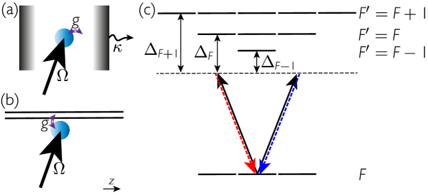
Figure 5: Setup. A single atom coupled strongly to (a) a cavity or (b) a waveguide is driven off resonantly at a Rabi frequency $\Omega$. The atom is coupled to the cavity or waveguide at a strength $g$, such that light is scattered by the atom off three detuned hyperfine levels into the cavity and waveguide. The cavity axis or waveguide is chosen as the quantization axis $z$, such that the drive and cavity and waveguide modes couple to $\sigma_{\pm}$-polarized transitions in the atom.

As in the main text, we consider an atom initialized in a hyperfine state $F$, with $2F+1$ magnetic sublevels $\set{-m,-m+1,\dots,m}$ and driven on the $D_{2}$ line by an arbitrary superposition of $\sigma_{\pm}$-polarized light. The atom can scatter into a cavity (or equivalently a waveguide) [see Figure 5]. The cavity has two modes with $\sigma_{\pm}$ polarization and degenerate frequency.

The system follows a master equation ($\hbar=1$)

$$\dot{\rho}=-{\rm i}[\hat{H},\rho]+\kappa\mathcal{L}[\hat{a}]\rho+\kappa\mathcal{L}[\hat{b}]\rho$$ (71)

where $\hat{a}~{}(\hat{b})$ is the annihilation operator for the $\sigma_{+}$ ($\sigma_{-}$) polarized cavity mode, $\mathcal{L}[\hat{O}]\rho=2\hat{O}\rho\hat{O}^{\dagger}-\hat{O}^{\dagger}\hat{O}\rho-\rho\hat{O}^{\dagger}\hat{O}$ and the total Hamiltonian is $\hat{H}=\hat{H}_{\mathrm{sys.}}+\hat{H}_{\mathrm{\mathrm{int.}}}$. In the rotating frame of the drive, the system Hamiltonian is

$$\hat{H}_{\mathrm{sys.}} =\delta\left(\hat{a}^{\dagger}\hat{a}+\hat{b}^{\dagger}\hat{b}\right)+\sum\limits_{F^{\prime}}\Delta_{F^{\prime}}\sum\limits_{m_{F^{\prime}}}\ket{F^{\prime},m_{F^{\prime}}}\bra{F^{\prime},m_{F^{\prime}}},$$ (72)

where $\delta=\omega-\omega_{c}$ is the detuning between drive and cavity mode, $\Delta_{F^{\prime}}=\omega-\omega_{F^{\prime}}$ is the detuning of the drive from the excited manifold $F^{\prime}$. We assume that all Zeeman shifts are negligible such that all magnetic sublevels can be considered at the same energy. The interaction Hamiltonian is

$$\hat{H}_{\mathrm{int.}}=\sum\limits_{F,F^{\prime}}\left(\frac{\cos\theta~{}\Omega}{2}+g\hat{a}\right)\sum\limits_{m}r^{m}_{F,F^{\prime}}\ket{F^{\prime},m+1}\bra{F,m}+\sum\limits_{F,F^{\prime}}\left(\frac{\sin\theta~{}\Omega}{2}+g\hat{b}\right)\sum\limits_{m}s^{m}_{F,F^{\prime}}\ket{F^{\prime},m-1}\bra{F,m}+\mathrm{H.c.},$$ (73)

where $\Omega$ is the Rabi frequency of the drive, $g$ is the coupling strength of the atom to the cavity and $\theta$ encodes the ellipticity of the drive, as in the main text.

In the limit of $\Omega_{\pm}/\Delta_{F^{\prime}}\ll 1~{}\forall~{}F^{\prime}$, the atomic saturation is essentially zero, and one can adiabatically eliminate the excited states. This yields an effective Hamiltonian

$$\hat{H}_{\mathrm{eff.}} =\delta(\hat{a}^{\dagger}\hat{a}+\hat{b}^{\dagger}\hat{b})+\sum\limits_{m}\left[\left(U_{m}^{a}\hat{a}^{\dagger}\hat{a}+U_{m}^{b}\hat{b}^{\dagger}\hat{b}+\omega_{m}\right)\ket{m}\bra{m}+\tilde{\Omega}_{m}\left(\ket{m+2}\bra{m}+\ket{m}\bra{m+2}\right)\right.$$

$$+h_{m}\left(\hat{b}^{\dagger}\hat{a}\ket{m+2}\bra{m}+\hat{a}^{\dagger}\hat{b}\ket{m}\bra{m+2}\right)+\eta^{+,\mathrm{Ray.}}_{m}\left(\hat{a}+\hat{a}^{\dagger}\right)\ket{m}\bra{m}+\eta^{-,\mathrm{Ray.}}_{m}\left(\hat{b}+\hat{b}^{\dagger}\right)\ket{m}\bra{m}$$

$$+\left.\cos\theta~{}\eta^{\mathrm{Ram.}}_{m}\left(\hat{b}^{\dagger}\ket{m+2}\bra{m}+\hat{b}\ket{m}\bra{m+2}\right)+\sin\theta~{}\eta^{\mathrm{Ram.}}_{m}\left(\hat{a}^{\dagger}\ket{m}\bra{m+2}+\hat{a}\ket{m+2}\bra{m}\right)\right],$$ (74)

where we have dropped the $F$ notation from the atomic states and defined various effective parameters. The effective frequency of the atomic states is given by the light shift from the drive laser and from cavity population

$$U_{m}^{a}=\sum\limits_{F^{\prime}}\frac{g^{2}r^{2}_{m,F,F^{\prime}}}{\Delta_{F^{\prime}}},\;\;\;\;U_{m}^{b}=\sum\limits_{F^{\prime}}\frac{g^{2}s^{2}_{m,F,F^{\prime}}}{\Delta_{F^{\prime}}},\;\;\;\;\omega_{m}=\sum\limits_{F^{\prime}}\frac{\Omega^{2}\left(\cos^{2}\theta~{}r^{2}_{m,F,F^{\prime}}+\sin^{2}\theta~{}s^{2}_{m,F,F^{\prime}}\right)}{4\Delta_{F^{\prime}}}.$$ (75)

There are also coupling terms between atomic states which conserve photon number. This corresponds to two-photon transitions mediated by two oppositely-polarized drive photons or the transfer of population between the two cavity modes. These processes occur at rates

$$\tilde{\Omega}_{m}=\sum\limits_{F^{\prime}}\frac{\cos\theta~{}\sin\theta~{}\Omega^{2}r_{m,F,F^{\prime}}s_{m+2,F,F^{\prime}}}{4\Delta_{F^{\prime}}},\;\;\;\;h_{m}=\sum\limits_{F^{\prime}}\frac{g^{2}r_{m,F,F^{\prime}}s_{m+2,F,F^{\prime}}}{\Delta_{F^{\prime}}}.$$ (76)

The final group of terms correspond to describe processes where the atoms scatter into the cavity. This can happen in two ways: returning to the same atomic state or changing atomic state. Employing the same designations of Rayleigh and Raman scattering as in the main text, these scattering rates read

$$\eta^{+,\mathrm{Ray.}}_{m}=\sum\limits_{F^{\prime}}\frac{\cos\theta~{}\Omega gr^{2}_{m,F,F^{\prime}}}{2\Delta_{F^{\prime}}},\;\;\;\;\eta^{-,\mathrm{Ray.}}_{m}=\sum\limits_{F^{\prime}}\frac{\sin\theta~{}\Omega gs^{2}_{m,F,F^{\prime}}}{2\Delta_{F^{\prime}}},\;\;\;\;\eta^{\mathrm{Ram.}}_{m}=\sum\limits_{F^{\prime}}\frac{\Omega gr_{m,F,F^{\prime}}s_{m+2,F,F^{\prime}}}{2\Delta_{F^{\prime}}}.$$ (77)

F.1 Simplifications at the magic detuning

It is convenient to transform the effective Hamiltonian into the parallel and perpendicular basis. These modes are composed of the circularly polarized modes as

$$\hat{c}_{\parallel}=\cos\theta~{}\hat{a}+\sin\theta~{}\hat{b},\;\;\;\;\;\;\hat{c}_{\perp}=\sin\theta~{}\hat{a}-\cos\theta~{}\hat{b}.$$ (78)

Using these expressions and assuming we operate at a magic detuning, the above Hamiltonian reads

$$H_{\mathrm{eff.}} =\delta\left(\hat{c}_{\parallel}^{\dagger}\hat{c}_{\parallel}+\hat{c}_{\perp}^{\dagger}\hat{c}_{\perp}\right)+\sum\limits_{m}\left[\left(U^{\parallel}\hat{c}_{\parallel}^{\dagger}\hat{c}_{\parallel}+U^{\perp}\hat{c}_{\perp}^{\dagger}\hat{c}_{\perp}+\omega_{m}\right)\ket{m}\bra{m}+\eta^{\parallel,\mathrm{Ray.}}\left(\hat{c}_{\parallel}+\hat{c}_{\parallel}^{\dagger}\right)\ket{m}\bra{m}\right]$$ (79)

$$=\left(\delta+U^{\parallel}\right)\hat{c}_{\parallel}^{\dagger}\hat{c}_{\parallel}+\left(\delta+U^{\perp}\right)\hat{c}_{\perp}^{\dagger}\hat{c}_{\perp}+\eta^{\parallel,\mathrm{Ray.}}\left(\hat{c}_{\parallel}+\hat{c}_{\parallel}^{\dagger}\right),$$ (80)

where we have defined new $m$-independent dispersive shifts and cavity scattering rates. These can be calculated for any choice of $m$ and take the form

$$U^{\parallel}=\cos^{2}\theta~{}U^{a}_{m}+\sin\theta^{2}~{}U^{b}_{m},\;\;\;\;U^{\perp}=\sin^{2}\theta~{}U^{a}_{m}+\cos^{2}\theta~{}U^{b}_{m},\;\;\;\;\eta^{\parallel,\mathrm{Ray.}}=\cos\theta~{}\eta^{+,\mathrm{Ray.}}_{m}+\sin\theta~{}\eta^{-,\mathrm{Ray.}}_{m}.$$ (81a)

In this form, the Hamiltonian reduces to that of an off-resonantly driven cavity. While the perpendicular cavity mode is also dispersively shifted, it does not play a role in dynamics. We thus write the single atom Hamiltonian as

$$H_{\mathrm{eff.}}=\left(\delta+U^{\parallel}\right)\hat{c}_{\parallel}^{\dagger}\hat{c}_{\parallel}+\eta^{\parallel,\mathrm{Ray.}}\left(\hat{c}_{\parallel}+\hat{c}_{\parallel}^{\dagger}\right).$$ (82)

We now consider $N$ atoms, each coupled to the cavity at $g_{j}=\sin\varphi_{j}g_{0}$, where $\varphi_{j}=\mathbf{k}_{c}\cdot\mathbf{r}_{j}$ encodes the strength of coupling between an atom at position $\mathbf{r}_{j}$ to a standing wave cavity mode with wavenumber $\mathbf{k}_{c}$. The Hamiltonian is then the sum over these $N$ atoms and gives

$$H_{\mathrm{eff.}}=\delta\hat{c}_{\parallel}^{\dagger}\hat{c}_{\parallel}+\sum\limits_{j=1}^{N}\sin^{2}\varphi_{j}~{}U^{\parallel}\hat{c}_{\parallel}^{\dagger}\hat{c}_{\parallel}+\sin\varphi_{j}~{}\eta^{\parallel,\mathrm{Ray.}}\left(\hat{c}_{\parallel}+\hat{c}_{\parallel}^{\dagger}\right).$$ (83)

If all atoms couple equally and in phase then $\sum_{j}\sin\varphi_{j}=N$, and the field intensity scales as $N^{2}$. If atoms couple equally but with alternating signs, then the sum is zero for an even number of atoms or one for an odd number. These results align with those observed in Ref. [42].

References

- Blatt and Roos [2012] R. Blatt and C. F. Roos, Quantum simulations with trapped ions, Nat. Phys. 8, 277 (2012).
- Bruzewicz et al. [2019] C. D. Bruzewicz, J. Chiaverini, R. McConnell, and J. M. Sage, Trapped-ion quantum computing: Progress and challenges, Appl. Phys. Rev. 6, 021314 (2019).
- Hammerer et al. [2010] K. Hammerer, A. S. Sørensen, and E. S. Polzik, Quantum interface between light and atomic ensembles, Rev. Mod. Phys. 82, 1041 (2010).
- Browaeys and Lahaye [2020] A. Browaeys and T. Lahaye, Many-body physics with individually controlled Rydberg atoms, Nat. Phys. 16, 132 (2020).
- Kjaergaard et al. [2020] M. Kjaergaard, M. E. Schwartz, J. Braumüller, P. Krantz, J. I. J. Wang, S. Gustavsson, and W. D. Oliver, Superconducting qubits: Current state of play, Annu. Rev. Condens. Matter Phys. 11, 369 (2020).
- Ren et al. [2019] S. Ren, Q. Tan, and J. Zhang, Review on the quantum emitters in two-dimensional materials, J. Semicond. 40, 071903 (2019).
- García de Arquer et al. [2021] F. P. García de Arquer, D. V. Talapin, V. I. Klimov, Y. Arakawa, M. Bayer, and E. H. Sargent, Semiconductor quantum dots: Technological progress and future challenges, Science 373, eaaz8541 (2021).
- Ladd et al. [2010] T. D. Ladd, F. Jelezko, R. Laflamme, Y. Nakamura, C. Monroe, and J. L. O’Brien, Quantum computers, Nature 464, 45 (2010).
- Preskill [2018] J. Preskill, Quantum computing in the NISQ era and beyond, Quantum 2, 79 (2018).
- Georgescu et al. [2014] I. M. Georgescu, S. Ashhab, and F. Nori, Quantum simulation, Rev. Mod. Phys. 86, 153 (2014).
- Altman et al. [2021] E. Altman, K. R. Brown, G. Carleo, L. D. Carr, E. Demler, C. Chin, B. DeMarco, S. E. Economou, M. A. Eriksson, K.-M. C. Fu, M. Greiner, K. R. Hazzard, R. G. Hulet, A. J. Kollár, B. L. Lev, M. D. Lukin, R. Ma, X. Mi, S. Misra, C. Monroe, K. Murch, Z. Nazario, K.-K. Ni, A. C. Potter, P. Roushan, M. Saffman, M. Schleier-Smith, I. Siddiqi, R. Simmonds, M. Singh, I. Spielman, K. Temme, D. S. Weiss, J. Vučković, V. Vuletić, J. Ye, and M. Zwierlein, Quantum simulators: Architectures and opportunities, PRX Quantum 2, 017003 (2021).
- Cronin et al. [2009] A. D. Cronin, J. Schmiedmayer, and D. E. Pritchard, Optics and interferometry with atoms and molecules, Rev. Mod. Phys. 81, 1051 (2009).
- Ma et al. [2011] J. Ma, X. Wang, C. Sun, and F. Nori, Quantum spin squeezing, Phys. Rep. 509, 89 (2011).
- Pezzè et al. [2018] L. Pezzè, A. Smerzi, M. K. Oberthaler, R. Schmied, and P. Treutlein, Quantum metrology with nonclassical states of atomic ensembles, Rev. Mod. Phys. 90, 035005 (2018).
- Birnbaum et al. [2006] K. M. Birnbaum, A. S. Parkins, and H. J. Kimble, Cavity QED with multiple hyperfine levels, Phys. Rev. A 74, 063802 (2006).
- Piñeiro Orioli et al. [2022] A. Piñeiro Orioli, J. K. Thompson, and A. M. Rey, Emergent dark states from superradiant dynamics in multilevel atoms in a cavity, Phys. Rev. X 12, 011054 (2022).
- Happer [1972] W. Happer, Optical pumping, Rev. Mod. Phys. 44, 169 (1972).
- Daley et al. [2008] A. J. Daley, M. M. Boyd, J. Ye, and P. Zoller, Quantum computing with alkaline-earth-metal atoms, Phys. Rev. Lett. 101, 170504 (2008).
- Gorshkov et al. [2009] A. V. Gorshkov, A. M. Rey, A. J. Daley, M. M. Boyd, J. Ye, P. Zoller, and M. D. Lukin, Alkaline-earth-metal atoms as few-qubit quantum registers, Phys. Rev. Lett. 102, 110503 (2009).
- Allcock et al. [2021] D. T. C. Allcock, W. C. Campbell, J. Chiaverini, I. L. Chuang, E. R. Hudson, I. D. Moore, A. Ransford, C. Roman, J. M. Sage, and D. J. Wineland, blueprint for trapped ion quantum computing with metastable states, Appl. Phys. Lett. 119, 214002 (2021).
- Chen et al. [2022] N. Chen, L. Li, W. Huie, M. Zhao, I. Vetter, C. H. Greene, and J. P. Covey, Analyzing the Rydberg-based optical-metastable-ground architecture for nuclear spins, Phys. Rev. A 105, 052438 (2022).
- Wu et al. [2022] Y. Wu, S. Kolkowitz, S. Puri, and J. D. Thompson, Erasure conversion for fault-tolerant quantum computing in alkaline earth Rydberg atom arrays, Nat. Commun. 13, 4657 (2022).
- Kang et al. [2023] M. Kang, W. C. Campbell, and K. R. Brown, Quantum error correction with metastable states of trapped ions using erasure conversion, PRX Quantum 4, 020358 (2023).
- Lis et al. [2023] J. W. Lis, A. Senoo, W. F. McGrew, F. Rönchen, A. Jenkins, and A. M. Kaufman, Mid-circuit operations using the omg-architecture in neutral atom arrays, arXiv:2305.19266 (2023).
- Sadler et al. [2006] L. E. Sadler, J. M. Higbie, S. R. Leslie, M. Vengalattore, and D. M. Stamper-Kurn, Spontaneous symmetry breaking in a quenched ferromagnetic spinor Bose-Einstein condensate, Nature 443, 312 (2006).
- Klempt et al. [2010] C. Klempt, O. Topic, G. Gebreyesus, M. Scherer, T. Henninger, P. Hyllus, W. Ertmer, L. Santos, and J. J. Arlt, Parametric amplification of vacuum fluctuations in a spinor condensate, Phys. Rev. Lett. 104, 195303 (2010).
- Hamley et al. [2012] C. D. Hamley, C. S. Gerving, T. M. Hoang, E. M. Bookjans, and M. S. Chapman, Spin-nematic squeezed vacuum in a quantum gas, Nat. Phys. 8, 305 (2012).
- Luo et al. [2017] X.-Y. Luo, Y.-Q. Zou, L.-N. Wu, Q. Liu, M.-F. Han, M. K. Tey, and L. You, Deterministic entanglement generation from driving through quantum phase transitions, Science 355, 620 (2017).
- Masson et al. [2017] S. J. Masson, M. D. Barrett, and S. Parkins, Cavity QED engineering of spin dynamics and squeezing in a spinor gas, Phys. Rev. Lett. 119, 213601 (2017).
- Zhang et al. [2017] Z. Zhang, C. H. Lee, R. Kumar, K. J. Arnold, S. J. Masson, A. S. Parkins, and M. D. Barrett, Nonequilibrium phase transition in a spin-1 Dicke model, Optica 4, 424 (2017).
- Davis et al. [2019] E. J. Davis, G. Bentsen, L. Homeier, T. Li, and M. H. Schleier-Smith, Photon-mediated spin-exchange dynamics of spin-1 atoms, Phys. Rev. Lett. 122, 010405 (2019).
- Periwal et al. [2021] A. Periwal, E. S. Cooper, P. Kunkel, J. F. Wienand, E. J. Davis, and M. Schleier-Smith, Programmable interactions and emergent geometry in an array of atom clouds, Nature 600, 630 (2021).
- Katori et al. [1999] H. Katori, T. Ido, and M. Kuwata-Gonokami, Optimal design of dipole potentials for efficient loading of sr atoms, J. Phys. Soc. Jpn. 68, 2479 (1999).
- McKeever et al. [2003] J. McKeever, J. R. Buck, A. D. Boozer, A. Kuzmich, H.-C. Nägerl, D. M. Stamper-Kurn, and H. J. Kimble, State-insensitive cooling and trapping of single atoms in an optical cavity, Phys. Rev. Lett. 90, 133602 (2003).
- Ye et al. [2008] J. Ye, H. J. Kimble, and H. Katori, Quantum state engineering and precision metrology using state-insensitive light traps, Science 320, 1734 (2008).
- Kim et al. [2013] H. Kim, H. S. Han, and D. Cho, Magic polarization for optical trapping of atoms without Stark-induced dephasing, Phys. Rev. Lett. 111, 243004 (2013).
- Kaur et al. [2015] J. Kaur, S. Singh, B. Arora, and B. K. Sahoo, Magic wavelengths in the alkaline-earth-metal ions, Phys. Rev. A 92, 031402 (2015).
- Katori et al. [2003] H. Katori, M. Takamoto, V. G. Pal’chikov, and V. D. Ovsiannikov, Ultrastable optical clock with neutral atoms in an engineered light shift trap, Phys. Rev. Lett. 91, 173005 (2003).
- Cooper et al. [2018] A. Cooper, J. P. Covey, I. S. Madjarov, S. G. Porsev, M. S. Safronova, and M. Endres, Alkaline-earth atoms in optical tweezers, Phys. Rev. X 8, 041055 (2018).
- Norcia et al. [2018] M. A. Norcia, A. W. Young, and A. M. Kaufman, Microscopic control and detection of ultracold strontium in optical-tweezer arrays, Phys. Rev. X 8, 041054 (2018).
- Saskin et al. [2019] S. Saskin, J. T. Wilson, B. Grinkemeyer, and J. D. Thompson, Narrow-line cooling and imaging of ytterbium atoms in an optical tweezer array, Phys. Rev. Lett. 122, 143002 (2019).
- Yan et al. [2023] Z. Yan, J. Ho, Y.-H. Lu, S. J. Masson, A. Asenjo-Garcia, and D. M. Stamper-Kurn, Super-radiant and sub-radiant cavity scattering by atom arrays, arXiv:2307.13321 (2023).
- Rosenbusch et al. [2009] P. Rosenbusch, S. Ghezali, V. A. Dzuba, V. V. Flambaum, K. Beloy, and A. Derevianko, ac Stark shift of the Cs microwave atomic clock transitions, Phys. Rev. A 79, 013404 (2009).
- Note [1] Note that this choice of polarization is not the same as that in Ref. [42], where it was assumed the (linear-polarized) drive was -polarized. Here, we choose a different polarization axis because it is more convenient for the algebra to work in the plane for arbitrary elliptical polarization. Of course, the physics is unaffected by this choice, and our results will hold for any polarization axis choice.
- Schwartz [1955] C. Schwartz, Theory of hyperfine structure, Phys. Rev. 97, 380 (1955).
- Allegrini et al. [2022] M. Allegrini, E. Arimondo, and L. A. Orozco, Survey of hyperfine structure measurements in alkali atoms, J. Phys. Chem. Ref. Data 51, 043102 (2022).
- Shimizu et al. [1987] F. Shimizu, K. Shimizu, Y.-i. Gomi, and H. Takuma, Direct observation of hyperfine splittings of the 7L 2P3/2 state by subnatural linewidth spectroscopy, Phys. Rev. A 35, 3149 (1987).
- Yei et al. [1993] W. Yei, A. Sieradzan, and M. D. Havey, Delayed-detection measurement of atomic Na 3p 2P3/2 hyperfine structure using polarization quantum-beat spectroscopy, Phys. Rev. A 48, 1909 (1993).
- Falke et al. [2006] S. Falke, E. Tiemann, C. Lisdat, H. Schnatz, and G. Grosche, Transition frequencies of the lines of , , and measured with a femtosecond laser frequency comb, Phys. Rev. A 74, 032503 (2006).
- Das and Natarajan [2008] D. Das and V. Natarajan, High-precision measurement of hyperfine structure in the D lines of alkali atoms, J. Phys. B 41, 035001 (2008).
- Ye et al. [1996] J. Ye, S. Swartz, P. Jungner, and J. L. Hall, Hyperfine structure and absolute frequency of the 87Rb 5P3/2 state, Opt. Lett. 21, 1280 (1996).
- Gerginov et al. [2003] V. Gerginov, A. Derevianko, and C. E. Tanner, Observation of the nuclear magnetic octupole moment of 133Cs, Phys. Rev. Lett. 91, 072501 (2003).
- Nörtershäuser et al. [1998] W. Nörtershäuser, K. Blaum, K. Icker, P. Müller, A. Schmitt, K. Wendt, and B. Wiche, Isotope shifts and hyperfine structure in the transitions in calcium II, Eur. Phys. J. D 2, 33 (1998).
- Buchinger et al. [1990] F. Buchinger, E. B. Ramsay, E. Arnold, W. Neu, R. Neugart, K. Wendt, R. E. Silverans, P. Lievens, L. Vermeeren, D. Berdichevsky, R. Fleming, D. W. L. Sprung, and G. Ulm, Systematics of nuclear ground state properties in by laser spectroscopy, Phys. Rev. C 41, 2883 (1990).
- Villemoes et al. [1993] P. Villemoes, A. Arnesen, F. Heijkenskjold, and A. Wannstrom, Isotope shifts and hyperfine structure of 134-138Ba II by fast ion beam-laser spectroscopy, J. Phys. B 26, 4289 (1993).
- Neu et al. [1988] W. Neu, R. Neugart, E. W. Otten, G. Passler, K. Wendt, B. Fricke, E. Arnold, H. J. Kluge, and G. Ulm, Quadrupole moments of radium isotopes from the hyperfine structure in Ra II, Z. Phys. D 11, 105 (1988).
- Baumann et al. [2010] K. Baumann, C. Guerlin, F. Brennecke, and T. Esslinger, Dicke quantum phase transition with a superfluid gas in an optical cavity, Nature 464, 1301 (2010).
- Baumann et al. [2011] K. Baumann, R. Mottl, F. Brennecke, and T. Esslinger, Exploring symmetry breaking at the Dicke quantum phase transition, Phys. Rev. Lett. 107, 140402 (2011).
- Klinder et al. [2015] J. Klinder, H. Keßler, M. Wolke, L. Mathey, and A. Hemmerich, Dynamical phase transition in the open Dicke model, Proc. Natl. Acad. Sci. USA 112, 3290 (2015).
- Vetsch et al. [2010] E. Vetsch, D. Reitz, G. Sagué, R. Schmidt, S. T. Dawkins, and A. Rauschenbeutel, Optical interface created by laser-cooled atoms trapped in the evanescent field surrounding an optical nanofiber, Phys. Rev. Lett. 104, 203603 (2010).
- Solano et al. [2017] P. Solano, P. Barberis-Blostein, F. K. Fatemi, L. A. Orozco, and S. L. Rolston, Super-radiance reveals infinite-range dipole interactions through a nanofiber, Nat. Commun. 8, 1857 (2017).
- Goban et al. [2015] A. Goban, C.-L. Hung, J. D. Hood, S.-P. Yu, J. A. Muniz, O. Painter, and H. J. Kimble, Superradiance for atoms trapped along a photonic crystal waveguide, Phys. Rev. Lett. 115, 063601 (2015).
- Fritzsche [2002] S. Fritzsche, Large-scale accurate structure calculations for open-shell atoms and ions, Physica Scripta 2002, 37 (2002).
- Bause et al. [2020] R. Bause, M. Li, A. Schindewolf, X.-Y. Chen, M. Duda, S. Kotochigova, I. Bloch, and X.-Y. Luo, Tune-out and magic wavelengths for ground-state molecules, Phys. Rev. Lett. 125, 023201 (2020).
- Guan et al. [2021] Q. Guan, S. L. Cornish, and S. Kotochigova, Magic conditions for multiple rotational states of bialkali molecules in optical lattices, Phys. Rev. A 103, 043311 (2021).