Entanglement and factorization in
axion-de Sitter universes

Abstract

We study Renyi entropies and late-time bulk correlators between asymptotically de Sitter space universes connected through an Euclidean axion wormhole in arbitrary dimensions. We first establish the notion of entropy with respect to these observers within the background-independent approach to the algebra of operators. We then provide an explicit derivation of holographic Renyi entropies between the universes considering the dS/CFT correspondence. In the quantum mechanical description, the results can be recasted in terms of reduced density matrix where one of the asymptotically dS universes is traced out. Remarkably, our work shows that the throat of the Euclidean wormhole is associated with the entanglement between the universes. Later, we study correlators for heavy particles in the presence of an observer. We find that the Euclidean wormhole saddle allows for the late-time correlators with respect to observers located in the asymptotically dS universes to achieve a constant value at late times, while for the disconnected saddles do not contribute. The result is compatible with each of the asymptotically de Sitter universes being described by a finite-dimensional quantum dual theory. Lastly, we provide with an effective theory description of the dimensional reduction of these geometries in terms of dilaton-gravity theory with conformally coupled matter.

newfloatplacementnewfloatnamenewfloatfileextnewfloatwithin

1 Introduction

Euclidean wormhole geometries are crucial to developing notions of generalized entropy in arbitrary spacetimes. However, it is notoriously difficult to produce these types of geometries for closed universes, such as in de Sitter (dS) space; where most known examples Balasubramanian:2020xqf ; Balasubramanian:2023xyd ; Mirbabayi:2023vgl have been introduced in lower dimensions. Recently, Aguilar-Gutierrez:2023ril studied the properties of Euclidean wormholes (of the Strominger-Giddings kind Giddings:1987cg ) saddle points to the gravitational path integral for asymptotically dS space geometries in higher dimensions in the presence of axion fluxes. See also Gutperle:2002km ; Chen:2016ask for related work.

One can construct a Lorentzian cosmology corresponding to the solutions in Aguilar-Gutierrez:2023ril by cutting the wormhole in half, either at the throat or at the location of the maximal scaling factor (see Fig. 2), which results in asymptotically dS universes connected through a quantum bounce, referring to a tunneling event, in the presence of axion matter content. The latter describes an ultra-stiff fluid, which has an equation of state $\rho=p$, denoting energy density and pressure respectively. Due to the presence of the wormhole, the universes seem to be entangled. However, it has not been explored how exactly they are entangled according to some appropriate measure of correlation between these systems, and what type of implications it would have for the (putative) dual theory. Moreover, there appears to be a factorization puzzle Maldacena:2001kr for the putative microscopic theory dual to the bulk explicit geometry, outside the context of AdS/CFT duality.

On the other hand, adding the observer in pure dS space has led to several developments Chandrasekaran:2022cip ; Witten:2023qsv where one can propose rigorous notions of entropy and entanglement, and a corresponding algebra of operators while considering the $G_{N}\rightarrow 0$ limit. This has been emphasized in several other works Gomez:2022eui ; Gomez:2023jbg ; Gomez:2023tkr ; Gomez:2023upk ; Gomez:2023wrq ; Seo:2022pqj ; Jensen:2023yxy ; Aguilar-Gutierrez:2023odp ; Balasubramanian:2023xyd ; Kudler-Flam:2023qfl for different closed universes. We would like to understand the role of the observer in quantum cosmology Hartle:2009ig with these recent developments. A particularly useful method in this pursuit is the background-independent approach Witten:2023xze , one has the guidance of the Hartle-Hawking (HH) preparation of state as the (conjectured) maximal entropy state, with some non-trivial checks.

In this work, we show that the pair universes are not independent of each other, and we propose how to qualify this entanglement. To define the concepts of entropy from this preparation of state, we rely on recent progress in developing a background-independent algebra of observables Witten:2023xze . The main hypotheses in this framework are that the HH state can be prepared for any background and that it represents the maximally entropic state with respect to a worldline observer. Although we also take the observer for granted in the theory; it might need to be part of the UV completion of the theory, rather than it being an external object.

Based on the hypothesis that the HH preparation of state provides a notion of maximally entropic state for a worldline observer, we evaluate the Renyi entropies according to $\mathcal{I}^{+}$ observers in the asymptotically dS universes using the framework of dS/CFT holography, where these measures of entropy can be deduced from the geometry of the wormhole connecting the universes. They lead to an arguably simple interpretation in terms of a putative dual theory living near $\mathcal{I}^{+}$. Given that each of the observers perceives the same entropy, this would mean that we have bi-partitioned a pure state of disconnected subsystems. According to the field theory dual, we can think about the state preparation from the Euclidean wormhole as generating individual thermal density matrices that are purified by its “twin” (i.e. auxiliary) universe, coupled through the wormhole. The geometric evaluation reveals that the throat of the Euclidean wormhole is responsible for providing non-trivial Renyi entropies to each of the disjoint universes.

One might associate the finite entropy for each of the universes in terms of a dual quantum mechanical system with a finite number of degrees of freedom. However, it has been discussed in several contexts that attaching such interpretations for pure dS space, also leads to obstacles. One instance is when performing the late time limit evaluation of bulk correlators. Different works find that correlators would decay exponentially with time and reach a vanishing value asymptotically, which conflicts with the results found for generic quantum mechanical systems with a finite number of degrees of freedom that one would associate with the finite entropy of dS space Dyson:2002nt . Progress in the holographic interpretation of the correlators for the Gibbons-Hawking saddle Gibbons:1976ue was recently done in Aalsma:2022eru ; Chapman:2022mqd . The discrepancy has been recently alleviated in Mirbabayi:2023vgl , who finds that including wormhole geometries in Euclidean anti-de Sitter (AdS₂) space and continuing to Lorentzian dS₂ space lead to a non-vanishing answer for the late time bulk correlators, in agreement with expectations. However, the discussion specializes in two dimensions given the technical challenges of finding these saddles to the Euclidean path integral in higher dimensions. In our work, we explore whether the Euclidean wormhole geometries produced with axion fluxes in asymptotically dS universes can indeed lead to the same type of conclusions in a higher dimensional case. We perform the explicit analysis in the geodesic approximation, where one considers heavy particle states propagating along a geodesic in the explicit axion-dS background geometry. Our results agree with the general expectations that the norm of correlators reaches a non-vanishing value at late times, associated with the finite Hilbert space dimensions for the dual theory.

Besides providing a higher dimensional example where the throat of the wormhole is associated with entanglement between universes, which also allows for a non-vanishing late time correlation; we will derive a two-dimensional dilaton gravity model describing the dimensional reduction of the three-dimensional axion-dS wormholes. Here the axion particles appear as conformally coupled matter. We denote the resulting theory axion-dS JT gravity. Given the several developments in JT gravity to study the information paradox Almheiri:2019psf ; Penington:2019npb , we hope that this reduced model will be useful to develop a better understanding of islands in asymptotically dS spacetimes.

Structure: In Sec. 2 we present general facts about the axion-dS universes, including the geometry, some special limiting cases, when the axion charge reaches a critical value allowed by the finite size of dS space, and the general 3D geometry. In Sec. 3 we explain how to define entropy between the axion-dS universes through the background independent proposal to algebras of observables Witten:2023xze . We then employ the concepts of dS/CFT holography Strominger:2001pn to perform the explicit computation of Renyi entropies, previously considered in pure dS space by Dong:2018cuv , and provide a dual field theory interpreation. Once we have established a finite entanglement entropy between the universes, Sec. 4 presents the behavior of late-time bulk correlators between pairs of geodesic observers between the universes in the probe approximation. We find the wormholes indeed lead to the expectation value of a late-time bulk correlator being a non-vanishing value for arbitrarily late times, in contrast to the disconnected saddles. In Sec. 5, we conclude with a summary of our work and some interesting future directions. Finally, App. A contains the dimensional reduction of the three-dimensional axion-dS universe, resulting in a dilaton gravity theory reproducing features of the corresponding (spatially closed) Friedmann–Lemaître–Robertson–Walker (FLRW) cosmology.

2 Brief review axion-de Sitter wormholes

Axion-dS wormholes were recently studied in detail in Aguilar-Gutierrez:2023ril (see also Gutperle:2002km ). This section reviews some general properties used for the following sections and sets the notation.

2.1 Euclidean formulation

The $D$-dimensional theory is formulated in Euclidean space, starting with Einstein gravity in the presence of axion matter content and a positive cosmological constant:

$$I=\int\quantity[-\frac{1}{2\kappa_{D}^{2}}\star(R-2\Lambda)+\frac{1}{2}\star H_{D-1}\wedge H_{D-1}]\leavevmode\nobreak\ ,$$ (1)

where $H_{D-1}$ is the axion flux field, which is Hodge dual to the axion field $\chi$ (i.e. $H_{D-1}=\star d\chi$); $\kappa_{D}^{2}=8\pi G_{N}$ and we will consider a cosmological constant

$$\Lambda=\frac{(D-1)(D-2)}{2\ell^{2}}>0\leavevmode\nobreak\ .$$ (2)

One can find spherical symmetric solutions of this theory with an ansatz,

$$\mathrm{d}s^{2} =N(\tau)^{2}\mathrm{d}\tau^{2}+a(\tau)^{2}\mathrm{d}\Omega_{D-1}^{2}\,.$$ (3)

The axion flux field adopts the form

$$H_{D-1}=Q\,\text{Vol}(\text{S}^{D-1})\leavevmode\nobreak\ ,$$ (4)

where $Q$ is a constant representing the axion flux density; and $\text{Vol}(\text{S}^{D-1})$ is the $(D-1)-$form volume element of the sphere, $\mathrm{d}\Omega_{D-1}^{2}$.

The Einstein equations then imply that the Euclidean scale factor $a(\tau)$ obeys the following constraint,

$$\frac{1}{N}\frac{\mathrm{d}a}{\mathrm{d}\tau}=\pm\sqrt{1-\frac{a^{2}}{\ell^{2}}-\frac{\kappa_{D}^{2}Q^{2}\,a^{-2(D-2)}}{(D-1)(D-2)}}\,.$$ (5)

The Euclidean manifold for spherically symmetric axion wormholes is S${}^{D-1}\times$S¹. The argument goes as follows. One can find the locations where $\derivative{a}{\tau}=0$ from the above, which indicate where the maximum and minimum values of the scale factor $a$ are located, the latter corresponds to the wormhole throat size. At these locations, we can smoothly glue the geometry by performing a periodic identification in the values of the scale factor. In principle, they can be also analytically continued to an integer factor of the periodicity for extended instanton solutions, however, they are suppressed Aguilar-Gutierrez:2023ril , and they do not play a role in our arguments. See Fig. 1 for an illustration of the Euclidean geometry. This means that the Euclidean time $\tau$ lives in a finite interval $\tau\in[\tau_{\rm min},\,\tau_{\rm max}]$, whose endpoints are periodically identified.

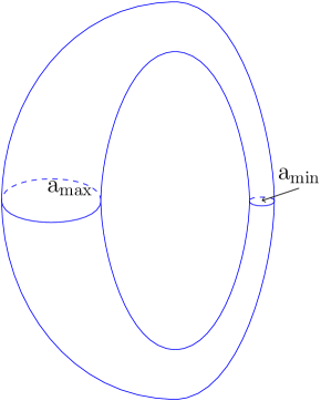
Figure 1: Euclidean geometry (in blue) of the axion-dS wormhole. The range of values of the scale factor $a\in[a_{\rm min},\leavevmode\nobreak\ a_{\rm max}]$ are determined by the roots of (5).

We now make a few remarks:

Nariai wormhole: The axion charge $Q$ cannot take arbitrarily large values, due to dS space being a closed universe. One can find a bound on the maximal through size for the wormholes, denoted by “Nariai wormhole”, by extremizing (5) with respect to $a$,

$$\kappa_{D}^{2}Q^{2}_{\rm max} =\ell^{2(D-2)}(D-2)\quantity(\frac{D-2}{D-1})^{D-2}\,,$$ (6)

$$a_{\text{max}}(Q_{\text{max}}) =a_{\text{min}}(Q_{\text{max}})=\sqrt{\frac{D-2}{D-1}}\ell\,.$$ (7)

Regular coordinates: The metric (3) might not capture the global geometry for a generic gauge parameter $N$, given that it can become undetermined at $\mathcal{H}=0$ surfaces. We look for a global coordinate system:

$$\mathrm{d}s^{2}=\mathrm{d}\tau^{2}+a(\tau)^{2}\mathrm{d}\Omega_{D-1}^{2}\leavevmode\nobreak\ .$$ (8)

The simplest case, where one can find analytic solutions for $a(\tau)$ in (8), is $D=3$. Taking $a(\tau=0)=a_{\rm max}$:

$$\mathrm{d}s^{2}=\mathrm{d}\tau^{2}+\frac{\ell^{2}}{2}\quantity(1-\cos(2\frac{\tau}{\ell})\sqrt{1-\frac{2\kappa_{3}^{2}Q^{2}}{\ell^{2}}})\mathrm{d}\Omega_{2}^{2}\leavevmode\nobreak\ .$$ (9)

Identifying the allowed range to cover the entire geometry, one sees that in this coordinate system $\tau\sim\tau+\pi/\ell$.

2.2 Lorentzian description

From the Euclidean geometry, one can also learn about Lorentzian evolution that emerges from the initial conditions specified by the HH state preparing two different universes connected through the same Euclidean saddle. A generalization of the HH proposal for this geometry was proposed in Aguilar-Gutierrez:2023ril . One slices the Euclidean geometry at either $a=a_{\rm max}$ or $a=a_{\rm min}$ and performs the Wick rotation. The initial conditions are then determined from the Euclidean path integral preparing the state. Moreover, by a careful treatment of the scalar inhomogeneities in the background, one can find that the resulting geometries have opposite pointing arrows of time, describing bouncing universes. The resulting Lorentzian in both cases is displayed in Fig. 2.

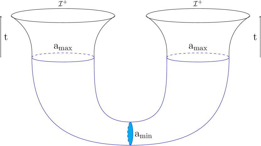
(a)

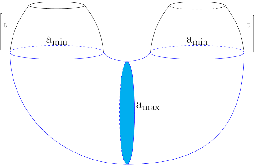
(b)

Figure 2: Hartle-Hawking preparation of the axion-dS universes constructed by slicing the geometry twice at (a) $a=a_{\rm max}$; (b) $a=a_{\rm min}$ (shown with different relative scales), (c) both $a=a_{\rm max}$ and $a=a_{\rm min}$. The Euclidean saddle is shown with blue lines and its Lorentzian evolution is in black, and a cyan disk bi-partitioning the system. The resulting universes flow with an inverted arrow of time one from the other, describing bouncing cosmologies.

The evolution of these universes follow from a simple Wick-rotation $\tau=\mathrm{i}t$, of (5), resulting in

$$\quantity(\frac{\dot{a}(t)}{N(t)\leavevmode\nobreak\ a(t)})^{2}=\frac{1}{\ell^{2}}-\frac{1}{a(t)^{2}}+\rho(t)\leavevmode\nobreak\ ,$$ (10)

$$\rho:=\frac{\kappa_{D}^{2}Q^{2}a^{-2(D-1)}}{(D-1)(D-2)}$$ (11)

where $\rho$ is the energy density of the axion particles, and the dot indicates differentiation. This simply represents a spatially closed FLRW cosmology; a positive cosmological constant; and axion particles, which have an equation of state $\rho=p$, the latter being the pressure.

Later, it will be useful to adopt a conformal gauge in (3) after Wick rotating $\tau\rightarrow\mathrm{i}t$,

$$\mathrm{d}s^{2}=a(t)^{2}\quantity(-\mathrm{d}t^{2}+\mathrm{d}\theta_{1}^{2}+\cos^{2}\theta_{1}\mathrm{d}\Omega_{D-2})\leavevmode\nobreak\ ,$$ (12)

where $0\leq t\leq\pi/2$ where $t=0$ corresponds to a quantum bounce (see App. B in Aguilar-Gutierrez:2023ril ), and $-\pi/2\leq\theta_{1}\leq\pi/2$.

Also important for us, the careful analysis of gauge invariant inhomogeneities in the Lorentzian-signature universes shows that the arrow of time, defined as the increase in deviations from homogeneity, gets invested between the two universes Aguilar-Gutierrez:2023ril .

3 Entropy from wormhole state preparation

In this section, we quantify the amount of entanglement between the dS universes coupled through the Euclidean wormhole in the presence of a worldline observer. We briefly motivate our arguments based on the hypothesis in the background-independent approach to algebras of observables Witten:2023xze . Having established the notion of entropy, we work on a specific framework, the dS/CFT correspondence Strominger:2001pn , to explicitly evaluate the gravitational entropy where the entangling region corresponds to $\mathcal{I}^{+}$ of a single one of the universes. For generality, we evaluate Renyi entropies in this framework. We then provide an interpretation from the field theoretical dual where the gravitational entropy corresponds to the entanglement entropy of a reduced density matrix where one of the universes is traced out with the dS/CFT framework.

3.1 Background independent approach

We now consider the entropy of an individual universe with respect to a worldline observer, following the background-independent approach to the algebra of observables Witten:2023xze . Here, it is assumed that the usual HH state, regardless of the particular spacetime, will always be a state (or weight) for the algebra of observables and that the HH state represents a maximally entropic state for a worldline observer moving along a geodesic. This is motivated by the HH state being the most universal way to prepare states in gravitational backgrounds from an Euclidean path integral, and it also has passed some consistency checks. One can then use this state to provide a notion of relative entropies for other states associated with the algebra of observables, independent of whether the particular type of von Neumann algebra recovered after assigning a Hilbert space representation for the system.

We will describe the state describing two copies of the HH no-boundary solution as $\ket{\psi_{\rm WHH}}$, which prepares the evolution of the universes with probe observers. This allow us to define the expectation values for all elements in the operator algebra with respect to a given observer in either copy.

In case one can associate a type I or II von Neumann algebra description to our system after choosing a Hilbert space representation, there is a corresponding to the reduced density matrix of a single axion-dS universe, $\rho_{\rm WHH}$, prepared from the HH state, and a corresponding entropy

$$S(\rho_{\rm WHH})=-\Tr\rho_{\rm WHH}\log\rho_{\rm WHH}\leavevmode\nobreak\ .$$ (13)

Having defined this entropy we now look for a explicit evaluation from the background geometry and field theory dual interpretation.

3.2 Holographic Renyi entropies

Geometrically, we have access to the entropy above according to a geodesic observer located on a single of the universes, depicted by the disks in Fig. 2. A natural way to identify the (13) with a bulk notion of entropy is through the dS/CFT correspondence Strominger:2001pn . In this framework, we can work out the gravitational Renyi entropy using the cosmic brane proposal Lewkowycz:2013nqa in the dS/CFT framework Dong:2018cuv . In this case, the Euclidean action for the whole system can be expressed as

$$I =I_{\rm bulk}+I_{\rm brane}\leavevmode\nobreak\ ,$$ (14)

$$I_{\rm brane} =T_{n}\int\sqrt{h}\leavevmode\nobreak\ \mathrm{d}^{D-2}y$$ (15)

and $h_{ij}$ is the (codimension-2) induced metric on the cosmic brane, with tension $T_{n}=\frac{n-1}{4nG_{N}}$. The Renyi entropies can be conveniently found following the procedure in Dong:2016fnf .

One defines a natural generalization of the usual Renyi entropies, ${S}_{n}$, through

$$\tilde{S}_{n}=-n^{2}\partial_{n}\quantity(\frac{n-1}{n}S_{n})\leavevmode\nobreak\ ,$$ (16)

where $\tilde{S}_{n}$ is identified with the area of a cosmic brane, $C_{n}$ for an entangling region near $\mathcal{I}^{+}$ of an asymptotically dS space Dong:2018cuv

$$\tilde{S}_{n}=\frac{A_{\mathbf{R}}(\rm C_{n})}{4G_{N}}\leavevmode\nobreak\ .$$ (17)

where $A(C_{n})$ is the area of the minimal codimension-2 surface of a cosmic string $C_{n}$ inserted on that surface homologous to the entangling region very close to $\mathcal{I}^{+}$ in Fig. 2 (a) for a single of the universes (left, or right), which we take to be S^D-1 for the geometry in (8). In contrast 2 (b) would correspond to a collapsing universe. The $n\rightarrow 1$ case then corresponds to the von Neumann entropy where the entangling surface near $\mathcal{I}^{+}$ corresponds to a single one of the universe.

Here, the presence of the axion particles on the geometry in the action (14) will be considered as the effective action backreacting in the geometry, such that we can trust in the identification of the entropy as the minimal area of a codimension-2 surface at this order.

To specify the evaluation region, we express

$$\mathrm{d}\Omega_{D-1}^{2}=\mathrm{d}\theta_{1}^{2}+\cos^{2}\theta_{1}\mathrm{d}\theta_{2}+\dots+\cos^{2}\theta_{1}\dots\cos^{2}\theta_{D-2}\mathrm{d}\theta_{D-1}^{2}\leavevmode\nobreak\ .$$ (18)

We must now also account for the backreaction of the cosmic string. Notice first that the addition of the codimension-2 term (14) can only modify the scale factor $a(\tau)$ through boundary conditions on the location of the cosmic string.

First notice that the homology constraint for the minimal area given the region S^D-1 near $\mathcal{I}^{+}$ requires that a surface S^D-2 is taken around the Euclidean wormhole, corresponding to $\theta_{D-1}=0$ in (18). The area functional reads

$$A(C_{n})=\int\mathrm{d}\Omega_{D-3}\int\mathrm{d}\sigma\sqrt{\quantity(\derivative{\tau}{\sigma})^{2}+a(\tau)^{2}\quantity(\derivative{\theta_{1}}{\sigma})^{2}}a(\tau)^{D-2}\quantity(\cos\theta_{1})^{D-2}\leavevmode\nobreak\ ,$$ (19)

where $\sigma$ is an arbitrary parametrization of the codimension-2 surface. From (19) it is clear that $a(\tau)=a(\tau=\tau_{\min})$ would provide the minimal area.

Then the contribution from the codimension-two brane is just

$$I_{\rm brane}=T_{n}\Omega_{D-2}a_{\rm min}^{D-2}\leavevmode\nobreak\ ,$$ (20)

which is necessarily just a constant; thus the cosmic brane will not contribute to the overall variation of the action, based on the symmetries of the problem. This means that the parameter $n$ will not modify the solution $a(\tau)$ in (5). Moreover, since the generalized Renyi entropy is independent of the parameter $n$, (16) implies that all the Renyi entropies are the same, so we will denote $S:=\tilde{S}_{n}=S_{n}$. They will be uniquely determined by the area of the surfaces at $\tau=\tau_{\rm min}$ and $\theta_{D-1}=0$, by

$${S}=\frac{\Omega_{D-2}a_{\rm min}^{D-2}}{4G_{N}}\leavevmode\nobreak\ ,$$ (21)

which agrees with the pure dS_D result (when $Q=0$).

In general, it might not be possible to evaluate the scale factor of the regular metric analytically to evaluate (21). However, this is exactly solvable for the $D=3$ wormhole, shown in (9); as well as the Nariai case in (7) for any $D$. Notice however, that the case $Q=Q_{\rm max}$ is the Einstein static universe, which is not asymptotically dS space, so (21) does not apply for this limiting case, although it might provide an approximate answer for $Q\sim Q_{\rm max}$.

3.3 Towards a dual theory interpretation

We now move on to interpreting the Renyi entropy from the perspective of a putative quantum theory dual living near $\mathcal{I}^{+}$, which we consider as a very weakly gravitating region for late times in the expanding saddle geometry (Fig. 2 (a)).

The finite entropy (21) suggests that the Hilbert space dimension of this theory is $\mathrm{e}^{{S}}$. Since the wormhole prepares an entropic state with the same entropy for each universe, the dual description suggest an equivalence to having a canonical ensemble for each theory which is purified by coupling the original universe through the wormhole to the “twin” axion-dS universe. This means an EPR pair of universes was generated through instanton effects. This shares similarities to previous approaches in entangling pairs of disjoint gravitating universes Balasubramanian:2021wgd ; Miyata:2021qsm ; Balasubramanian:2023xyd .

The entropy calculated through (21) would then correspond to the Renyi entropy for the reduced density matrix of a single universe. Then it seems reasonable to view the von Neumann entropy ($n\rightarrow 1$) with respect to the observers near $\mathcal{I}^{+}$ as entanglement entropy due to the Euclidean wormhole in the Lorentzian cosmology. We have depicted this interpretation in Fig. 3 using the coordinates (12).

Figure 3: Spatially closed FLRW universes with an ultra-stiff fluid. The Euclidean wormhole preparation of state allows for entanglement between them.

To conclude this section, although so far we have been focused on the saddle Fig. 2 (a), there is yet another preparation of state where we cut the axion-dS wormhole of Fig. 1 not just at $a=a_{\rm max}$ and $a=a_{\rm min}$, but both at the same time and perform the Wick rotation $\tau\rightarrow\mathrm{i}t$.

The resulting geometry is illustrated in Fig. 4. It corresponds to collapsing and expanding FLRW cosmologies prepared through a Euclidean wormhole.

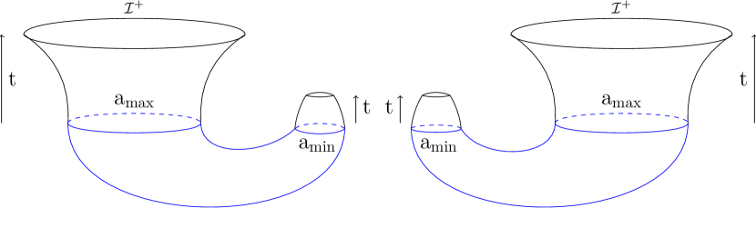
Figure 4: Four copy HH state preparation for collapsing and expanding universes, where the expanding branches are now uncoupled.

In this case, it is simple to compute the Renyi entropies corresponding to a single one of the pairs of expanding-coupled-to-collapsing universes following the homology constraint and minimization. The result is exactly as (21), meaning that the throat of the wormhole again determines the entropy respect to the $\mathcal{I}^{+}$ region once we have traced out the disconnected copy.

4 Late-time correlators

Since each of the axion-dS universes has a finite entropy, it could be described by a finite quantum system. On general grounds, it is expected that correlation functions must fluctuate at late proper times with respect to a worldline observer in these systems, leading to a non-vanishing norm for the late-time correlators; while the Gibbons-Hawking saddle displays correlators that decay exponentially at late times Dyson:2002nt , indicating that there should be saddle points contributing to the correlators, or that there might be some conflict between the low-energy description with the finite quantum system interpretation. This point of view was emphasized in Mirbabayi:2023vgl , which found a new Lorentzian saddle for dS JT gravity was found by making an analytic continuation from the double cone in EAdS JT gravity. This new saddle shows that one can restore the late-time behavior of correlation functions which is compatible with the finite entropy; although it has only been found in two dimensions.

In this section, we investigate whether the presence of the Euclidean wormhole between dS universes can lead to a late-time correlator consistent with these expectations in higher dimensions.

4.1 Geodesic approximation

We now add a massive free scalar field, $\phi$, in the axion-dS wormhole plus universe configuration (Fig. 2), where the scalar theory is given:

$$I_{\rm scalar}=-\frac{1}{2}\int\mathrm{d}^{D}x\sqrt{-g}\leavevmode\nobreak\ \quantity(\quantity(\partial\phi)^{2}+m^{2}\phi^{2})\leavevmode\nobreak\ .$$ (22)

We can then compute its propagator in different ways. We will employ the geodesic approximation, valid when $\phi$ is a heavy massive field Balasubramanian:1999zv ; Louko:2000tp , which has been recently discussed by Chapman:2022mqd ; Aalsma:2022eru ; Faruk:2023uzs in the context of complex geodesics in dS space. Here

$$G(x,\leavevmode\nobreak\ y)\simeq\sum_{g\in\text{geodesics}}\mathrm{e}^{-{m}\leavevmode\nobreak\ L^{\rm(g)}(x,\leavevmode\nobreak\ y)}$$ (23)

where $L^{\rm(g)}(x,\leavevmode\nobreak\ y)$ is the geodesic legth between the points $x$, $y$. This can be derived through path integrals and heat kernel methods. Also, (23) becomes more accurate when the points $x$ and $y$ are close to each other. We will consider 1-loop corrections to account for possible deviations from this regime.

4.2 Disconnected expanding universes

Let us start considering the disconnected saddle point geometry in Fig. 4. It is clear that if we locate the points $x$ and $y$ near $\mathcal{I}^{+}$ in the disconnected universes in Fig. 4 there cannot be any correlation between the two asymptotically dS region. Geometrically, there is no geodesic connecting $x$ and $y$. In that case

$$G^{(\rm disc)}(x,\leavevmode\nobreak\ y)=0\leavevmode\nobreak\ .$$ (24)

However, this is puzzling, since we found a non-zero entropy for this system according to (21). A possibility is that the effective bulk description does not reproduce the fine details of the quantum mechanical theory. However, it is also known in the context of the factorization puzzle Maldacena:2001kr and baby universes Anous:2020lka that one needs to account for connected geometries to obtain an answer consistent with the finite Hilbert space interpretation.

4.3 Connected expanding universes

Next, we will compare this result with the the late-time correlator for the pair of observers close to $\mathcal{I}^{+}$ in each of the universes shown in Fig 5 with a propagator passing through the wormhole geometry.

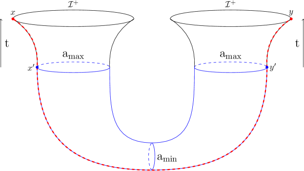
Figure 5: Correlator for very heavy fields following a geodesic (red dashed line) between points $x$ and $y$ (red dots) very near $\mathcal{I}^{+}$ on each axion-dS universe, and they are connected by a geodesic path to $x^{\prime}$, $y^{\prime}$ (blue dots) to the Euclidean wormhole.

Let us denote the Lorentzian contributions to the geodesic length with $L^{\rm(g)}(z_{i},\leavevmode\nobreak\ z_{i}^{\prime})$, and $z_{i}=\quantity{x,\leavevmode\nobreak\ y}$, $z^{\prime}_{i}=\quantity{x^{\prime},\leavevmode\nobreak\ y^{\prime}}$, and the Euclidean part as $L^{\rm(g)}(x^{\prime},\leavevmode\nobreak\ y^{\prime})$.

To specify the region of evaluation, we consider that the points $x$, $y$ in the “twin” universes, are located in the coordinate $t$, $\quantity{\theta_{i}}$ (8) although in different universes, where the arrow of time is inverted (see Sec. 2.2). The geodesic equation requires the same for the points $x^{\prime}$, $y^{\prime}$ in the $a=a_{\rm max}$ slice of the Euclidean wormholes.

We start the evaluation with the sections $x$ to $x^{\prime}$, and $y$ to $y^{\prime}$ in Fig 5. Considering the Wick rotation $\tau\rightarrow\mathrm{i}t$ in (8), so we can specify the geodesic length in these patches as

$$L^{\rm(g)}(z_{i},\leavevmode\nobreak\ z_{i}^{\prime})=\int_{\lambda_{z_{i}}}^{\lambda_{z_{i}^{\prime}}}\mathrm{d}\lambda\leavevmode\nobreak\ \sqrt{-\quantity(\derivative{t}{\lambda})^{2}+a(t(\lambda))^{2}\quantity(\derivative{\Omega_{D-1}}{\lambda})^{2}}\leavevmode\nobreak\ ,$$ (25)

where $\lambda$ is a general parametrization for the geodesic.

However, recall the inversion in the time flow mentioned in Sec. 2. Since we employ spatial symmetric points for $x$, $y$, as well $x^{\prime}$ and $y$, we have that $\lambda_{x}=\lambda_{y}$ and $\lambda_{x^{\prime}}=\lambda_{y^{\prime}}$. This means that $L^{\rm(g)}(x,\leavevmode\nobreak\ x^{\prime})+L^{\rm(g)}(y,\leavevmode\nobreak\ y^{\prime})=0$, and thus only the Euclidean contribution remains

$$L^{\rm(g)}(x,\leavevmode\nobreak\ y)=L^{\rm(g)}(x^{\prime},\leavevmode\nobreak\ y^{\prime})\leavevmode\nobreak\ .$$ (26)

For the Euclidean section, we will use $\tau$ to parameterize the geodesic path, such that (8) has a corresponding length functional

$$L=\int\mathrm{d}\tau\leavevmode\nobreak\ \sqrt{1+a(\tau)^{2}\quantity(\derivative{\Omega_{D-1}}{\tau})^{2}}\leavevmode\nobreak\ .$$ (27)

For this particular calculation, we set the endpoints of the geodesics at $\theta_{i}(\tau=\tau_{\rm max})=0$ $\forall\leavevmode\nobreak\ 1\leq i\leq D-1$. The geodesic equations of motion

$$\partialderivative{L}{\theta_{i}}=\partial_{\tau}\partialderivative{L}{\dot{\theta}_{i}}\leavevmode\nobreak\ ,$$ (28)

can be used to verify that

$$\theta_{i}^{\rm(g)}=0,\quad 1\leq i\leq D-1$$ (29)

is the only solution to the geodesic equations respecting the boundary conditions. For this geodesic path the functional (27) is evaluated as

$$L^{\rm(g)}(x^{\prime},\leavevmode\nobreak\ y^{\prime})=\Delta\tau\leavevmode\nobreak\ ,\quad\Delta\tau\equiv 2\absolutevalue{\tau_{\rm max}-\tau_{\rm min}}\leavevmode\nobreak\ ,$$ (30)

which is just the periodicity of the wormhole. The corresponding propagator at tree-level in the geodesic approximation (23) is then

$$G^{\rm(conn)}(x,\leavevmode\nobreak\ y)\sim\mathrm{e}^{-2m\absolutevalue{\tau_{\rm max}-\tau_{\rm min}}}$$ (31)

generically.

One can also add 1-loop corrections for the evaluation of (23) as outlined in Chapman:2022mqd . We will study small deviations from the geodesic path (29) considering $\theta_{i}=\theta_{i}^{\rm(g)}+\delta\theta_{i}(\tau)$ with $\delta\theta_{i}(\tau)\ll 1$. In this case (27) has a corresponding second-order variation

$$\delta L=\int\mathrm{d}\tau\leavevmode\nobreak\ \frac{a(\tau)^{2}}{2}\sum_{i=1}^{D-1}\quantity(\derivative{\delta\theta_{i}}{\tau})^{2}\leavevmode\nobreak\ .$$ (32)

Then the 1-loop corrections to (23) can be evaluated through path integral methods

$$G^{\rm(conn)}(x,\leavevmode\nobreak\ y)=\sum_{g\in\text{geodesics}}\mathrm{e}^{-{m}\leavevmode\nobreak\ L^{\rm(g)}}\int\prod_{i=1}^{D-1}[d\delta\theta_{i}]\mathrm{e}^{-m\leavevmode\nobreak\ \delta L}\leavevmode\nobreak\ .$$ (33)

Combining (32) and (33), one can use the general path integral evaluation in App. C of Chapman:2022mqd to derive that

$$G^{\rm(conn)}(x,\leavevmode\nobreak\ y)=\mathrm{e}^{-m\Delta\tau}\sqrt{\frac{m}{2\pi f(\tau_{\rm min},\leavevmode\nobreak\ \tau_{\rm max})}}\leavevmode\nobreak\ ,$$ (34)

$$f(\tau_{\rm min},\leavevmode\nobreak\ \tau_{\rm max})=\int_{\tau_{\rm min}}^{\tau_{\rm max}}\frac{\mathrm{d}\tau}{a(\tau)^{2}}\leavevmode\nobreak\ .$$

In principle, the analytic evaluation of (34) for a generic wormhole can be done numerically for a scale factor $a(\tau)$ in regular coordinates; and it can be done analytically for the $D=3$ case in (9). For higher dimensions, we can illustrate the result by working in the regime where $Q\sim Q_{\rm max}$, such that $a(\tau)$ is approximately the constant (7). In that case (34) becomes

$$\evaluated{G^{\rm(conn)}(x,\leavevmode\nobreak\ y)}_{Q\sim Q_{\rm max}}=\mathrm{e}^{-m\Delta\tau}\sqrt{\frac{2}{\pi}\frac{(D-2)m\ell^{2}}{(D-1)\Delta\tau}}\leavevmode\nobreak\ .$$ (35)

Thus, we have recovered a finite answer for the late time behavior for $G(x,\leavevmode\nobreak\ y)$ in the effective field theory bulk description, which is consistent with the expectation of a dual theory with a finite number of degrees of freedom $\mathrm{e}^{S}$, with $S$ given in (21).

We conclude the section with a few remarks.

First, while we have evaluated the connected propagator in (34), given that we have both the disconnected saddles, Fig. 4, as well the connected ones in Fig. 2 (expanding and collapsing universes shown), then the contribution of the connected saddle to the full propagator will be suppressed by a factor $\sim\mathrm{e}^{I_{\rm on}^{(\rm conn)}-I_{\rm on}^{(\rm disc)}}$ with respect to disconnected saddle, where $I_{\rm on}^{(\rm disc)}=I_{\rm on}^{(\rm conn)}/2<0$ denote the on-shell actions of the disconnected and connected saddles. The on-shell actions for the axion-dS wormhole can be found in Aguilar-Gutierrez:2023ril .

Second, notice that for (35) we studied a case with exact symmetry in the operator insertions at $x$ and $y$ between the universes of Fig. 5 for simplicity. The inversion of the arrow of time plays an important role, such that only the Euclidean wormhole length plays a role in deriving the corresponding geodesic length. This is perhaps the most natural configuration to consider given the similarity to the late-time correlators between antipodal observers in pure dS space, which also show quasi-periodic decaying behavior Aalsma:2022eru , in contrast to the original formulation of the information paradox in the eternal AdS black hole Maldacena:2001kr .

5 Conclusions

Let us first summarize the work. We employed the background independent approach to algebras of operators Witten:2023xze to propose a notion of entanglement between universes prepared through a Lorentzian continuation from a Euclidean axion wormhole with a positive cosmological constant. We assume that the HH preparation with the wormhole produces a maximally entropic state in each universe. We explicitly computed the Renyi entropies corresponding to this configuration assuming a dS/CFT correspondence and we interpreted the result as a canonical ensemble of maximally mixed matter at $\mathcal{I}^{+}$ prepared through the wormhole. Importantly, the wormhole throat size controls all the Renyi entropies in this framework, providing a new perspective on holography for asymptotically dS spacetimes.

In order to test whether the finite entropy might have an interpretation as that of a finite-dimensional quantum system describing each of the universes, we calculated late-time correlators with respect to observers near $\mathcal{I}^{+}$ of the asymptotically dS universes, considering both disconnected, Fig. 4, and connected saddles Fig. 5. We showed that, in the geodesic approximation to correlators, the behavior of the late-time correlator in this configuration is just a finite constant, which is compatible with the expectations of an asymptotically dS space with finite entropy being described by a corresponding quantum mechanical theory with finite Hilbert space dimension. Thus, the coupling between the universes, through the Euclidean wormhole allows for a non-vanishing value for the correlator connecting the different universes in the late-time regime. In contrast, a similar evaluation in dS₂ JT gravity, the effective field theory description does not reproduce the expected behavior for $G(x,\leavevmode\nobreak\ y)$ (vanishing at late times), while $\absolutevalue{G(x,\leavevmode\nobreak\ y)}^{2}$ remains non-vanishing Mirbabayi:2023vgl .

We now discuss some important future directions related to this work.

First, the quantum information theory has allowed much progress in understanding non-factorization for general field theries with gravity duals. It would be very interesting to study in detail the intrinsic correlations between the axion-dS universes and wormholes in terms of Coleman’s original work Coleman:1988cy ; Coleman:1988tj using this techniques. Perhaps the recent progress on geometric quantum discord as a diagnostic of factorization Banerjee:2023liw in terms of a state ensembles would be worth pursuing to formulate this interpretation.

Secondly, we have been considering the observer in the probe limit to calculate the bulk correlators with respect to the observers in the axion-dS universes. However, Mirbabayi:2023vgl explicitly required a backreacting observer for the new saddle leading to $\absolutevalue{G(\tau)}\neq 0$ to appear. Perhaps the apparent differences in our cases are just features of the particular types of theories we studied. It would be interesting to study if our wormhole saddle survives after the introduction of a backreacting observer with more degrees of freedom, such as an AdS black hole introduced in Balasubramanian:2023xyd .

Thirdly, while we motivated some of the arguments for the precise entanglement between the axion-dS universes using the background independent approach to algebras of observables, given that we have a precise background one can study the type of von Neumann algebra this system might correspond to. For that, we would evaluate the trace of operators in the algebra using density matrices from the two-copy HH state, after implementing the isometries of the system and a Hamiltonian constraint accounting for the observer.

Fourth, the fact that the universes are entangled suggests that information is mutually encoded between them, with an inverted arrow of time. This is similar to false vacuum decay eternal inflation in quantum cosmology, where there is some redundancy in the description of the theory producing different multiverse bubbles Hartle:2016tpo . Perhaps our explicit model would be useful to study a notion of quantum error correction between the pair of universes.

Another closely related and natural direction to pursue would be to study entanglement and correlators for axion-AdS space. However, it has been noticed that there are possible inconsistencies with the holographic dictionary if the Euclidean wormholes end on multiple boundaries Hertog:2017owm ; Loges:2023ypl , and the Lorentzian interpretation remains more unclear than the setting we have been considering.

Finally, instead of the $\mathcal{I}^{+}$ view, one can study a holographic description of the particle horizon of the FLRW cosmology, similar to the Fischler-Susskind model Fischler:1998st ; Diaz:2007mh . However, it remains unclear the relation between the opposite universes if one only considers the particle horizon, unless it can encode information about the wormhole. In that case, the views might be compatible. It would be very interesting to study this connection with an appropriate quantum mechanical theory dual. It might also be interesting to study if some explicit approaches in dS space, such as Hikida:2022ltr , could be modified to include axions matter.

Appendix A Axion-dS JT gravity

In the following, $D=3$ quantities are denoted with hats, and two-dimensional ones are unhatted and have Latin indices.

We perform the dimensional reduction of axion-dS₃ space to a 2D dilaton gravity theory, which we call axion-dS JT gravity. We start with the Euclidean theory (1) in $D=3$

$$I_{\rm bulk}=-\int\mathrm{d}^{3}x\sqrt{\hat{g}}\quantity[\frac{1}{2\kappa_{3}^{2}}(\hat{\mathcal{R}}-2\Lambda)+\frac{1}{2}(\hat{\nabla}\chi)^{2}]$$ (36)

which we dimensionally reduce to two-dimensions

$$\mathrm{d}s^{2}=g_{ij}\mathrm{d}x^{i}\mathrm{d}x^{j}+\Phi^{2}\mathrm{d}\varphi^{2}\leavevmode\nobreak\ .$$ (37)

Using the explicit three-dimensional metric in (9), the dilaton can be identified as:

$$\Phi(\tau,\,\theta)=a(\tau)\sin\theta\leavevmode\nobreak\ .$$ (38)

The effective action becomes

$$I_{\rm bulk}=-2\pi\int\mathrm{d}^{2}x\sqrt{g}\Phi\quantity[\frac{1}{2\kappa_{3}^{2}}(\mathcal{R}^{(2)}-2\Lambda)+\rho]\leavevmode\nobreak\ .$$ (39)

where $\rho:=\frac{1}{2}(\hat{\nabla}\chi)^{2}=\frac{Q^{2}}{2a^{4}}$ is the energy density of the (massless) axion field.

The equations of motion for the lower dimensional system (39)

$$R=2\Lambda+16\pi G_{3}\rho\leavevmode\nobreak\ ,$$ (40)

$$- (\nabla_{i}\nabla_{j}-g_{ij}\nabla^{2})\Phi+\Lambda g_{ij}\Phi=8\pi G_{3}\Phi T_{ij}\leavevmode\nobreak\ ,$$

which are consistent with (5).

Although we have focused on the Euclidean theory; the continuation to the Lorentzian signature simply describes a spatially closed FLRW cosmology, positive cosmological constant, and an equation of state $p=\rho$, with a corresponding stress tensor

$$T_{ij}=pg_{ij}+(\rho+p)u_{i}u_{j}\leavevmode\nobreak\ .$$ (41)

The resulting 2D theory is a special case of a dilaton gravity theory where axion particles are conformally coupled matter. Two-dimensional FLRW gravity models have been previously studied in JT gravity in Cadoni:2002pu .

References

- (1) V. Balasubramanian, A. Kar and T. Ugajin, Islands in de Sitter space, JHEP 02 (2021) 072 [2008.05275].
- (2) V. Balasubramanian, Y. Nomura and T. Ugajin, de Sitter space is sometimes not empty, 2308.09748.
- (3) M. Mirbabayi, An Observer’s Measure of De Sitter Entropy, 2311.07724.
- (4) S.E. Aguilar-Gutierrez, T. Hertog, R. Tielemans, J.P. van der Schaar and T. Van Riet, Axion-de Sitter wormholes, JHEP 11 (2023) 225 [2306.13951].
- (5) S.B. Giddings and A. Strominger, Axion Induced Topology Change in Quantum Gravity and String Theory, Nucl. Phys. B 306 (1988) 890.
- (6) M. Gutperle and W. Sabra, Instantons and wormholes in Minkowski and (A)dS spaces, Nucl. Phys. B 647 (2002) 344 [hep-th/0206153].
- (7) P. Chen, Y.-C. Hu and D.-h. Yeom, Fuzzy Euclidean wormholes in de Sitter space, JCAP 07 (2017) 001 [1611.08468].
- (8) J.M. Maldacena, Eternal black holes in anti-de Sitter, JHEP 04 (2003) 021 [hep-th/0106112].
- (9) V. Chandrasekaran, R. Longo, G. Penington and E. Witten, An algebra of observables for de Sitter space, JHEP 02 (2023) 082 [2206.10780].
- (10) E. Witten, Algebras, Regions, and Observers, 2303.02837.
- (11) C. Gomez, Cosmology as a Crossed Product, 2207.06704.
- (12) C. Gomez, On the algebraic meaning of quantum gravity for closed Universes, 2311.01952.
- (13) C. Gomez, Traces and Time: a de Sitter Black Hole correspondence, 2307.01841.
- (14) C. Gomez, Clocks, Algebras and Cosmology, 2304.11845.
- (15) C. Gomez, Entanglement, Observers and Cosmology: a view from von Neumann Algebras, 2302.14747.
- (16) M.-S. Seo, Von Neumann algebra description of inflationary cosmology, Eur. Phys. J. C 83 (2023) 1003 [2212.05637].
- (17) K. Jensen, J. Sorce and A. Speranza, Generalized entropy for general subregions in quantum gravity, 2306.01837.
- (18) S.E. Aguilar-Gutierrez, E. Bahiru and R. Espíndola, The centaur-algebra of observables, 2307.04233.
- (19) J. Kudler-Flam, S. Leutheusser and G. Satishchandran, Generalized Black Hole Entropy is von Neumann Entropy, 2309.15897.
- (20) J. Hartle and T. Hertog, Replication Regulates Volume Weighting in Quantum Cosmology, Phys. Rev. D 80 (2009) 063531 [0905.3877].
- (21) E. Witten, A Background Independent Algebra in Quantum Gravity, 2308.03663.
- (22) L. Dyson, J. Lindesay and L. Susskind, Is there really a de Sitter/CFT duality?, JHEP 08 (2002) 045 [hep-th/0202163].
- (23) G.W. Gibbons and S.W. Hawking, Action Integrals and Partition Functions in Quantum Gravity, Phys. Rev. D 15 (1977) 2752.
- (24) L. Aalsma, M.M. Faruk, J.P. van der Schaar, M. Visser and J. de Witte, Late-Time Correlators and Complex Geodesics in de Sitter Space, 2212.01394.
- (25) S. Chapman, D.A. Galante, E. Harris, S.U. Sheorey and D. Vegh, Complex geodesics in de Sitter space, JHEP 03 (2023) 006 [2212.01398].
- (26) A. Almheiri, N. Engelhardt, D. Marolf and H. Maxfield, The entropy of bulk quantum fields and the entanglement wedge of an evaporating black hole, JHEP 12 (2019) 063 [1905.08762].
- (27) G. Penington, Entanglement Wedge Reconstruction and the Information Paradox, JHEP 09 (2020) 002 [1905.08255].
- (28) A. Strominger, The dS / CFT correspondence, JHEP 10 (2001) 034 [hep-th/0106113].
- (29) X. Dong, E. Silverstein and G. Torroba, De Sitter Holography and Entanglement Entropy, JHEP 07 (2018) 050 [1804.08623].
- (30) Y. Chen, V. Gorbenko and J. Maldacena, Bra-ket wormholes in gravitationally prepared states, JHEP 02 (2021) 009 [2007.16091].
- (31) A. Milekhin and A. Tajdini, Bra-ket wormholes and Casimir entropy, 2212.08246.
- (32) A. Lewkowycz and J. Maldacena, Generalized gravitational entropy, JHEP 08 (2013) 090 [1304.4926].
- (33) X. Dong, J. Kudler-Flam and P. Rath, A Modified Cosmic Brane Proposal for Holographic Renyi Entropy, 2312.04625.
- (34) J. Kastikainen and A. Svesko, Gravitational Rényi entropy from corner terms, 2312.06765.
- (35) X. Dong, The Gravity Dual of Renyi Entropy, Nature Commun. 7 (2016) 12472 [1601.06788].
- (36) S.E. Aguilar-Gutierrez, A.K. Patra and J.F. Pedraza, Entangled universes in dS wedge holography, JHEP 10 (2023) 156 [2308.05666].
- (37) S.E. Aguilar-Gutierrez and F. Landgren, A multiverse model in dS wedge holography, 2311.02074.
- (38) J. Garriga, Nucleation rates in flat and curved space, Phys. Rev. D 49 (1994) 6327 [hep-ph/9308280].
- (39) M. Arcos, W. Fischler, J.F. Pedraza and A. Svesko, Membrane nucleation rates from holography, JHEP 12 (2022) 141 [2207.06447].
- (40) V. Balasubramanian, A. Kar and T. Ugajin, Entanglement between two gravitating universes, Class. Quant. Grav. 39 (2022) 174001 [2104.13383].
- (41) A. Miyata and T. Ugajin, Entanglement between two evaporating black holes, JHEP 09 (2022) 009 [2111.11688].
- (42) V. Balasubramanian and S.F. Ross, Holographic particle detection, Phys. Rev. D 61 (2000) 044007 [hep-th/9906226].
- (43) J. Louko, D. Marolf and S.F. Ross, On geodesic propagators and black hole holography, Phys. Rev. D 62 (2000) 044041 [hep-th/0002111].
- (44) M.M. Faruk, E. Morvan and J.P. van der Schaar, Static sphere observers and geodesics in Schwarzschild-de Sitter spacetime, 2312.06878.
- (45) T. Anous, J. Kruthoff and R. Mahajan, Density matrices in quantum gravity, SciPost Phys. 9 (2020) 045 [2006.17000].
- (46) M. Kontsevich and G. Segal, Wick Rotation and the Positivity of Energy in Quantum Field Theory, Quart. J. Math. Oxford Ser. 72 (2021) 673 [2105.10161].
- (47) E. Witten, A Note On Complex Spacetime Metrics, 2111.06514.
- (48) S.R. Coleman, Black Holes as Red Herrings: Topological Fluctuations and the Loss of Quantum Coherence, Nucl. Phys. B 307 (1988) 867.
- (49) S.R. Coleman, Why There Is Nothing Rather Than Something: A Theory of the Cosmological Constant, Nucl. Phys. B 310 (1988) 643.
- (50) S. Banerjee, P. Basteiro, R.N. Das and M. Dorband, Geometric quantum discord signals non-factorization, JHEP 08 (2023) 104 [2305.04952].
- (51) J. Hartle and T. Hertog, One Bubble to Rule Them All, Phys. Rev. D 95 (2017) 123502 [1604.03580].
- (52) T. Hertog, M. Trigiante and T. Van Riet, Axion Wormholes in AdS Compactifications, JHEP 06 (2017) 067 [1702.04622].
- (53) G.J. Loges, G. Shiu and T. Van Riet, A 10d construction of Euclidean axion wormholes in flat and AdS space, 2302.03688.
- (54) W. Fischler and L. Susskind, Holography and cosmology, hep-th/9806039.
- (55) P. Diaz, M.A. Per and A. Segui, Fischler-Susskind holographic cosmology revisited, Class. Quant. Grav. 24 (2007) 5595 [0704.1637].
- (56) Y. Hikida, T. Nishioka, T. Takayanagi and Y. Taki, CFT duals of three-dimensional de Sitter gravity, JHEP 05 (2022) 129 [2203.02852].
- (57) M. Cadoni and S. Mignemi, Cosmology of the Jackiw-Teitelboim model, Gen. Rel. Grav. 34 (2002) 2101 [gr-qc/0202066].