\setbeamertemplate

caption[numbered] \setbeamerfontcaptionsize= \setbeamertemplatefootline[frame number] \setbeamertemplatenavigation symbols \setbeamercolorpalette primarybg=white,fg=black \setbeamercolorstructurefg=RED \setbeamercolorsubsection in head/footbg=lightgrey,fg=Purple \defbeamertemplate*footlineinfolines {beamercolorbox}[wd=.3ht=2.25ex,dp=1ex,center]author in head/foot\usebeamerfontauthor in head/foot{beamercolorbox}[wd=.5ht=2.25ex,dp=1ex,center]title in head/foot\usebeamerfonttitle in head/foot{beamercolorbox}[wd=.2ht=2.25ex,dp=1ex,right]date in head/foot\usebeamerfontdate in head/foot       0 /     \beamertemplatenavigationsymbolsempty ]MiSoC Advisory Board Meeting
November 15, 2023 \institute[shortinst]\inst1Institute for Social and Economic Research (ISER), University of Essex and \inst2 Institute of Analytics and Data Science (IADS), University of Essex

[Uncaptioned image]
[Uncaptioned image]
[Uncaptioned image]

Machine Learning in a nutshell

  • Machine Learning (ML) algorithms are powerful predictive and classification tools in AI and Computer Science

    • e.g., penalized regression, tree-based approaches, neural networks

    • or text analysis, image analysis

  • Why ML?

    • Advantages: complexity reduction, flexibility, model selection

    • Disadvantages: interpretability, depending on hyperparameter tuning, stopping rules (regularisation), cross-validation to avoid overfitting, computationally intensive

    \beamergotobuttonExample with CART

ML and the social sciences

  • In social sciences, increasing attention to use ML potential for causal inference

    • e.g., in labour economics (davis2017; lechner2019; knaus2022heterogeneous; cengiz2022), health economics (heiler2021; difrancesco2022), environmental economics (klosin2022; stetter2022)

  • We focus on the use of ML in more traditional econometrics/statistics

    • By using generic ML methods to learn models, but using OLS/GMM to retrieve causal effect (e.g., belloni2016; chernozhukov2018; nie2021; chernozhukov2022)

    • Not building/modifying learning algorithms (e.g. atheyimbens2016; atheywager2018; atheytibshirani2019; kunzel2019; lechner2022)

  • We use ML to boost existing statistical estimation approaches for observational panel data

    • Specifically, to learn nuisance parameters of the confounders

The causal model for panel data

  • We consider robinson1988’s partially linear regression model for panel data

    $$y_{it}=d_{it}\theta+{\color\definecolor[named]{pgfstrokecolor}{rgb}{1,0,0}g(\mathbf{x}_{it})}+\alpha_{i}+u_{it},$$

    under $\mathbb{E}(\alpha_{i}|d_{it},\mathbf{x}_{it})\neq 0$ (i.e. fixed effects assumption)

  • Need to control for confounders, but $g(\mathbf{x}_{it})$ unknown

    • What variables? How many?

    • Linear or nonlinear?

  • Use ML tools (e.g., Lasso, trees, random forests) to get $\widehat{g}(\mathbf{x}_{it})$

The ML plug-in problem

  • Estimating $\theta$ from $$y_{it}=d_{it}\theta+{\color\definecolor[named]{pgfstrokecolor}{rgb}{1,0,0}\widehat{g}(\mathbf{x}_{it})}+\alpha_{i}+u_{it},$$ but regularization and/or overfitting bias leads to $\sqrt{n}(\widehat{\theta}-\theta)\not\rightarrow 0$
    (i.e. standard asymptotics invalid)
  • Double ML (DML) by chernozhukov2018

    1. 1.

      Sample splitting

    2. 2.

      Orthogonalisation of the estimating equations for $\theta$

  • DML in two-stages:

    1. 1.

      Learn nuisance parameters from each data fold \beamergotobuttonStage1

    2. 2.

      Solve the sample analogue of the moment condition wrt $\theta$.
      Average over folds attenuates ML bias and ensures $\sqrt{n}(\widehat{\theta}-\theta)\rightarrow 0$.
      \beamergotobuttonStage2\beamergotobuttonVariance

The estimators for panel data

  • Estimate $\theta$ consistently from

    $$y_{it}=d_{it}\theta+g(\mathbf{x}_{it})+{\color\definecolor[named]{pgfstrokecolor}{rgb}{1,0,0}\alpha_{i}}+u_{it},$$
    • under $\mathbb{E}(\alpha_{i}|d_{it},\mathbf{x}_{it})\neq 0$ (i.e. fixed effects assumption)

    • $g(\mathbf{x}_{it})$ may be non-linear in $\mathbf{x}$

  • We develop CRE, WG and FD estimators
    \beamergotobuttonCRE\beamergotobuttonWG/FD-hybrid\beamergotobuttonWG/FD-approx

  • These are based on mundlak1978’s model for fixed effect

    • Requires model assumptions for $\alpha_{i}$

    • Flexible way of predicting the treatment

Results

  • Bias reduction with CART/RF/Lasso with extended dictionary even for very non-linear functions, unlike OLS and Lasso w/t dictionary \beamergotobuttonPlots

  • Tree-based approaches under-estimate SD of sampling distribution

    • Estimators not normally distributed \beamergotobuttonDistributions

    • Sensitivity to hyperparameter tuning (machlanski2023) \beamergotobuttonTuning

  • Same behaviour when applying DML to observational panel data \beamergotobuttonApplication

  • Overall, ML are powerfull tools to approximate complex functional forms, but beware learner mismatch (“Don’t use sledgehammer to crack nut”)

Summary and future research

  • This setting is simple but raised many challenges for ML

    • Non-linearity of the nuisance parameters

    • Presence of fixed effects

  • Within the panel data framework, move on to

    • Heterogeneous treatment effects following nie2021

    • CATEs (e.g., interactive regression model by chernozhukov2018)

    • Dynamic panel models (cf semenova2023)

  • Allow for any learner within the context of DML (not only Lasso)

  • Apply the method to other empirical questions

    • Impact of minimum wage on employment, voting behaviour, mental health, etc.

    • Impact of maternal smoking on child’s outcomes at birth

    • Other possible applications …

Thank you for your attention!

[Uncaptioned image]
[Uncaptioned image]
[Uncaptioned image]
[Uncaptioned image]

References

CART \beamergotobuttonBackmissing

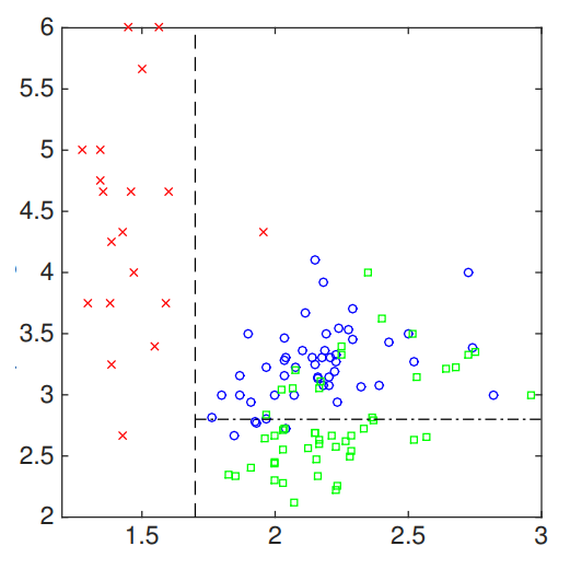
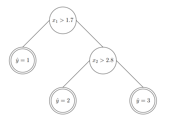
An simple illustration of a regression tree

CART \beamergotobuttonBackmissing

Refer to caption
(c)

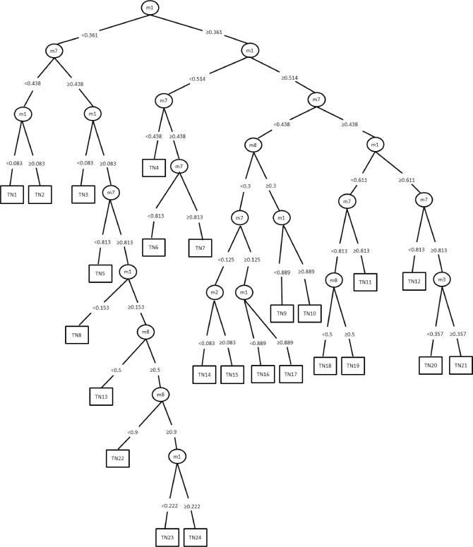
Source: yang2017. ‘A regression tree approach using mathematical programming’.

Hyperparameter tuning \beamergotobuttonBackmissing

Learner Hyperparamters Value/interval Description
Lasso lambda.min $\lambda$ equivalent to minimum mean cross-validated error
CART cp {0.01,0.02} Prune all nodes with a complexity less than cp from the printout.
minbucket {5,ceiling(N/2)} Minimum number of observations in any terminal leaf node.
minsplit minbucket$\times$3 Minimal node size to split at.
maxdepth {1,10} Maximum depth of any node of the final tree.
RF num.trees {5,100} Number of trees in the forest.
min.node.size {5,ceiling(N/2)} Minimal node size to split at.
max.depth {1,10} Maximum depth of any node of the final tree.
mtry $p$ The number of covariates, randomly sampled, to split at each node.
importance impurity The ‘impurity’ measure is the Gini index for classification,
the variance of the responses for regression and the sum of test statistics.
  • Note: Hyperparameter tuning for CART and RF is conducted with a random grid search. For RF, nodes with size smaller than min.node.size can occur.

CRE or Mundlak’s Device \beamergotobuttonBackmissing

  • mundlak1978 assumes $\mathbb{E}(\alpha_{i}|\mathbf{w}_{it})=\overline{\mathbf{w}}_{i}\bm{\beta}$
    where $\overline{\mathbf{w}}_{i}=T^{-1}\sum_{t=1}^{T}\mathbf{w}_{it}$

  • Only works for nonlinear case if $l(.)$ known (i.e. oracle)

  • Instead, we show equivalent learning problem is

    $\displaystyle y_{it}=v_{it}\theta+l_{2}(\mathbf{x}_{it},\overline{\mathbf{x}}_{i})+{\color\definecolor[named]{pgfstrokecolor}{rgb}{1,0,0}r_{i}}+u_{it}$ (1)
    $\displaystyle v_{it}=d_{it}-m_{2}(\mathbf{x}_{it},\overline{\mathbf{x}}_{i},\overline{d}_{i}),$ (2)

    provided

    • $\alpha_{i}=\overline{\mathbf{x}}_{i}^{\prime}\bm{\delta}+{\color\definecolor[named]{pgfstrokecolor}{rgb}{1,0,0}r_{i}}$

    • Additively separable $d_{it}=m_{1}(\mathbf{x}_{it},\overline{\mathbf{x}}_{i})+c_{i}+v_{it}$
      $\implies m_{2}(\mathbf{x}_{it},\overline{\mathbf{x}}_{i},\overline{d}_{i})=m_{1}(\mathbf{x}_{it},\overline{\mathbf{x}}_{i})+\overline{d}_{i}\pi-\overline{m}_{1}(\overline{\mathbf{x}}_{i})$

WG and FD Transformations \beamergotobuttonBackmissing

  • Within-group (WG): $\widetilde{w}_{it}=w_{it}-T^{-1}\sum_{s=1}^{T}w_{is}$

    $\displaystyle\widetilde{y}_{it}=\widetilde{d}_{it}\theta+\widetilde{l}(\mathbf{x}_{it})+\widetilde{u}_{it}$ (3)
    $\displaystyle\widetilde{v}_{it}=\widetilde{d}_{it}-\widetilde{m}(\mathbf{x}_{it})$ (4)

    $\widetilde{l}(\mathbf{x}_{it})\equiv l(\mathbf{x}_{it})-T^{-1}\sum_{s=1}^{T}l(\mathbf{x}_{is})\approx l(\widetilde{\mathbf{x}}_{it})$
    $\widetilde{m}(\mathbf{x}_{it})\equiv m(\mathbf{x}_{it})-T^{-1}\sum_{s=1}^{T}m(\mathbf{x}_{is})\approx m(\widetilde{\mathbf{x}}_{it})$

  • First-difference (FD): $\Delta w_{it}=w_{it}-w_{it-1}$

    $\displaystyle\Delta y_{it}=\Delta d_{it}\theta+\Delta l(\mathbf{x}_{it})+\Delta u_{it}$ (5)
    $\displaystyle\Delta v_{it}=\Delta d_{it}-\Delta m(\mathbf{x}_{it})$ (6)

    for $t=2,\dots,T$
    $\Delta l(\mathbf{x}_{it})\equiv l(\mathbf{x}_{it})-l(\mathbf{x}_{it-1})\approx l(\Delta\mathbf{x}_{it})$
    $\Delta m(\mathbf{x}_{it})\equiv m(\mathbf{x}_{it})-m(\mathbf{x}_{it-1})\approx m(\Delta\mathbf{x}_{it})$

Hybrid alternative for WG and FD estimators \beamergotobuttonBack

  1. 1.

    Learn $l(\mathbf{x}_{it})$ and $m(\mathbf{x}_{it})$ using mundlak1978’s device for CRE

  2. 2.

    Apply WG or FD transformation to $\widehat{l}(\mathbf{x}_{it})$ and $\widehat{m}(\mathbf{x}_{it})$

    • WG transformation:
      $\widetilde{l}\widehat{(\mathbf{x}_{it})}=\widehat{l}(\mathbf{x}_{it})-T^{-1}\sum_{s=1}^{T}\widehat{l}(\mathbf{x}_{is})$
      $\widetilde{m}\widehat{(\mathbf{x}_{it})}=\widehat{m}(\mathbf{x}_{it})-T^{-1}\sum_{s=1}^{T}\widehat{m}(\mathbf{x}_{is})$

    • FD transformation:
      $\Delta\widehat{l(\mathbf{x}_{it})}=\widehat{l}(\mathbf{x}_{it})-\widehat{l}(\mathbf{x}_{it-1})$
      $\Delta\widehat{m(\mathbf{x}_{it})}=\widehat{m}(\mathbf{x}_{it})-\widehat{m}(\mathbf{x}_{it-1})$

Estimating $\theta$ with DML: Stage 1 \beamergotobuttonBackmissing

  • Split the sample $\mathcal{W}$ in $k$ folds s.t.

    • Unit $i\in\mathcal{W}_{k}\Rightarrow i\notin\mathcal{W}_{k}^{c}$

    • Unit $i$ is observed for $T_{i}$ time periods

  • Learn the nuisance parameters $\eta=(l,m)$ for each fold using $i\notin\mathcal{W}_{k}$

  • Plug $\widehat{\eta}_{k}$ in the orthogonal score for the $k$-th fold

    $$\footnotesize\psi(\widetilde{W}_{it};\theta,\eta_{k})=\big{(}\widetilde{d}_{it}-\widetilde{m}(.)_{k}\big{)}\Big{\{}\big{(}\widetilde{y}_{it}-\widetilde{l}(.)_{k}-\big{(}\widetilde{d}_{it}-\widetilde{m}(.)_{k}\big{)}\theta\Big{\}}$$ (7)

    for all $i\in\mathcal{W}_{k}$ and $t\in S_{i}$, where $\widetilde{m}(.)=\mathbb{E}\big{(}\widetilde{d}_{it}|\widetilde{\mathbf{x}}_{it}\big{)}$ and $\widetilde{l}(.)=\mathbb{E}\big{(}\widetilde{y}_{it}|\widetilde{\mathbf{x}}_{it}\big{)}$

Estimating $\theta$ with DML: Stage 2 \beamergotobuttonBackmissing

  • By chernozhukov2018’s Lemma (2.6), $\theta$ satisfies

    $$\footnotesize\mathbb{E}\big{[}\psi(\widetilde{W};\theta,\eta)\big{]}=0$$ (8)
  • $\widehat{\theta}$ solves the finite-sample analog of (8) for each fold $k$

    $$\footnotesize\frac{1}{|\mathcal{W}_{k}|}\sum_{i\in\mathcal{W}_{k}}\sum_{t\in S_{i}}\psi(\widetilde{W}_{it};\theta,\widehat{\eta}_{k})=0$$ (9)

    with closed-form solution

    $$\scriptsize\widehat{\theta}_{k}=\Bigg{(}\frac{1}{|\mathcal{W}_{k}|}\sum_{i\in\mathcal{W}_{k}}\sum_{t\in S_{i}}\widehat{v}_{it}^{2}\Bigg{)}^{-1}\frac{1}{|\mathcal{W}_{k}|}\sum_{i\in\mathcal{W}_{k}}\sum_{t\in S_{i}}\widehat{v}_{it}\Big{(}\widetilde{y}_{it}-\widetilde{l}\widehat{(.)}_{k}\Big{)}$$ (10)

    where $\widehat{v}_{it}=\widetilde{d}_{it}-\widetilde{m}\widehat{(.)}_{k}$.

  • Average over all $k$ folds to get DML estimator of $\theta$

Inference with DML \beamergotobuttonBackmissing

  • The estimator of the cluster-robust variance is

    $$\widehat{\sigma}^{2}=\widehat{J}_{0}^{-1}\Bigg{[}\frac{1}{|\mathcal{W}_{k}|}\sum_{i\in\mathcal{W}_{k}}^{N}\sum_{t\in S_{i}}\psi(\widetilde{W}_{it};\theta,\widehat{\eta}_{k})\psi(\widetilde{W}_{it};\theta,\widehat{\eta}_{k})^{\prime}\Bigg{]}\widehat{J}_{0}^{-1}$$

    where $\widehat{J}_{0}=\frac{1}{|\mathcal{W}_{k}|}\sum_{i\in\mathcal{W}_{k}}^{N}\sum_{t\in S_{i}}\big{(}\widetilde{d}_{it}-\widetilde{m}\widehat{(.)}\big{)}^{2}\,\,\,\forall\,k=1,\dots,K$

MC Simulation results \beamergotobuttonBackmissing

[Uncaptioned image]

1¿[scale=.8]figs/dot_1408_cre_dgp_cnt.pdf [Uncaptioned image]2¿[scale=.8]figs/dot_1408_fe_dgp_cnt.pdf [Uncaptioned image]3¿[scale=.8]figs/dot_1408_fd_dgp_cnt.pdf Note: Averages over 100 Monte Carlo replications. DGP1 is linear in the nuisance functions; DGP2 smooth non-linear; DGP3 non-smooth non-linear. Time if fixed to $t=10$ time periods.

Sampling distribution of $\widehat{\theta}$ \beamergotobuttonBackmissing

[Uncaptioned image]

1¿[scale=.825]figs/kdensity_dgp_cre_cnt.pdf [Uncaptioned image]2¿[scale=.825]figs/kdensity_hybrid_dgp_wg_cnt.pdf [Uncaptioned image]3¿[scale=.8]figs/kdensity_hybrid_dgp_fd_cnt.pdf

Application with National Minimum Wage \beamergotobuttonBackmissing

  • We re-asses ‘Minimum wage and tolerance for high incomes’ by fazio2023 using DML for panel data

  • We replicate Specification (2) in Table (5)

    • Investigating voting behaviour after the introduction of the National Minimum Wage (NMW) in the UK in 1999.

    • They find that having benefited from the NMW raises the probability of voting conservative parties.

  • Data: British Household Panel Survey (BHPS)

OLS OLS DML-Lasso DML-Lasso DML-CART DML-RF
(1) (2) (3) (4) (5) (6)
Dependent variable: “Vote conservative”
NMW 0.097** 0.088** 0.093*** 0.079** 0.089** 0.149
(0.045) (0.045) (0.045) (0.045) (0.05) (0.127)
No. Observations 19,961 19,961 19,961 19,961 19,961 19,961
No. Groups 4,927 4,927 4,927 4,927 4,927 4,927
Controls vars Yes Yes Yes Yes Yes Yes
Wave FE Yes Yes Yes Yes Yes Yes
Region FE Yes Yes Yes Yes Yes Yes
Wave x Region FE No Yes No Yes No No
Resampling Information
Estimator WG WG WG-hybrid WGG-hybrid WGG-hybrid WGG-hybrid
No. folds 5 5 5 5
Folds per cluster 5 5 5 5
No. repeated sample splits 1 1 1 1
Cross-fitting Yes Yes Yes Yes
Score PO PO PO PO
DML algorithm 2 2 2 2
  • Note: Column (1) reports the figures of Specification (2) in Table 5 in fazio2023 estimated using least squares; Column (2) is LS regression with controls from Column (1) and interaction terms between wave and region fixed effects; remaining columns use DML with different (tuned) learners. Control variables include: age, education, marital status, household size, income of other members, and their individual means. Age squared and is included in Columns (1)-(3). Standard errors (in parenthesis) are clustered at the individual level. * p $<$ 0.10, ** p $<$ 0.05, *** p $<$ 0.01. \beamergotobuttonBack