Structure, variability, and origin of the low-latitude nightglow continuum between 300 and 1,800 nm: Evidence for HO_2 emission in the near-infrared

Abstract

The Earth’s mesopause region between about 75 and 105 km is characterised by chemiluminescent emission from various lines of different molecules and atoms. This emission was and is important for the study of the chemistry and dynamics in this altitude region at nighttime. However, our understanding is still very limited with respect to molecular emissions with low intensities and high line densities that are challenging to resolve. Based on 10 years of data from the astronomical X-shooter echelle spectrograph at Cerro Paranal in Chile, we have characterised in detail this nightglow (pseudo-)continuum in the wavelength range from 300 to 1,800 nm. We studied the spectral features, derived continuum components with similar variability, calculated climatologies, studied the response to solar activity, and even estimated the effective emission heights. The results indicate that the nightglow continuum at Cerro Paranal essentially consists of only two components, which exhibit very different properties. The main structures of these components peak at 595 and 1,510 nm. While the former was previously identified as the main peak of the FeO ‘orange arc’ bands, the latter is a new discovery. Laboratory data and theory indicate that this feature and other structures between about 800 and at least 1,800 nm are caused by emission from the low-lying A^′′ and A^′ states of HO_2. In order to test this assumption, we performed runs with the Whole Atmosphere Community Climate Model (WACCM) with modified chemistry and found that the total intensity, layer profile, and variability indeed support this interpretation, where the excited HO_2 radicals are mostly produced from the termolecular recombination of H and O_2. The WACCM results for the continuum component that dominates at visual wavelengths show good agreement for FeO from the reaction of Fe and O_3. However, the simulated total emission appears to be too low, which would require additional mechanisms where the variability is dominated by O_3. A possible (but nevertheless insufficient) process could be the production of excited OFeOH by the reaction of FeOH and O_3.

[Introduction]

At wavelengths shorter than about 1,800 nm, the Earth’s atmospheric radiation at nighttime is essentially caused by non-thermal chemiluminescence, i.e. photon emission by excited atomic and molecular states that are populated as a result of chemical reactions. Most of this nightglow emission originates at altitudes between 75 and 105 km in the mesopause region. The most prominent emitting species are the hydroxyl radical (OH) and molecular oxygen (O_2), which cause various ro-vibrational bands of emission lines from the near-ultraviolet (near-UV) to the near-infrared (near-IR) (rousselot00; cosby06; noll12). Especially strong emission is found above 1,400 nm, where OH bands of the electronic ground level with a vibrational level change $\Delta v$ of 2, e.g. OH(3-1), are located. Bands with higher $\Delta v$ that can be found at shorter wavelengths are significantly weaker. Strong emission is also related to O_2(b-X)(0-0) near 762 nm and O_2(a-X)(0-0) near 1,270 nm. However, both bands suffer from strong self-absorption in the lower atmosphere, which makes it particularly challenging to observe any emission of the former band from the ground. Intrinsically weaker but not self-absorbed O_2 bands are (b-X)(0-1) near 865 nm and O_2(a-X)(0-1) near 1,580 nm. Moreover, there are many weak O_2 bands at near-UV and blue wavelengths (slanger03; cosby06). In addition, especially the visual range shows atomic emission lines. Prominent examples are the atomic oxygen (O) lines at 558, 630, and 636 nm and the sodium (Na) doublet at 589 nm (e.g., cosby06; noll12).

Apart from individual emission lines, which have a typical width of a few picometres, the nightglow also includes an underlying continuum component. It could consist of line emissions if there were such a high line density that even spectroscopic instruments with high resolving power were not able to distinguish individual lines, i.e. it would be a pseudo-continuum. In any case, the observation of such a (pseudo-)continuum is more challenging than the study of well-resolved emission lines. The applied instrument needs to have a sufficiently high resolving power to clearly separate the continuum from the well-known emission bands and lines. As the continuum can be quite faint compared to the strong lines, even the wings of the line-spread function and possible straylight inside the instrument can be an issue, together with low signal-to-noise ratios. Moreover, part of the night-sky radiance is related to extraterrestrial light sources and scattering inside the atmosphere (e.g., leinert98). In particular, scattered moonlight, integrated and scattered starlight, zodiacal light, and possible light pollution can be significant sources of radiation. Hence, such components (which might be quite uncertain) need to be subtracted to measure the nightglow continuum (e.g., sternberg72; noll12; trinh13).

Despite the potential difficulties, barbier51 first noted a possible continuum in the green wavelength range. In the subsequent decades, additional constraints were found for a continuum in the visual wavelength range between 400 and 720 nm (davis65; broadfoot68; sternberg72; gadsden73; mcdade86), where the density of strong emission lines is relatively low. This continuum appeared to have a flux of several Rayleigh per nanometre (R nm^-1) with an increasing trend towards longer wavelengths and a possible local maximum (or at least plateau) near 600 nm (e.g., gadsden73). krassovsky51 already proposed that this continuum could be produced by the reaction NO + O →NO_2 + hν. The emission produced by this reaction, termed the NO_2 air afterglow, was observed in laboratory discharge experiments and has a pressure-dependent maximum, which is located around 580 nm for relevant atmospheric densities (fontijn64; becker72). Space-based measurements of the emission profile showed a peak between 90 to 95 km (savigny99; gattinger09; gattinger10; semenov14a). First indicated by ship-based latitude-dependent measurements (davis65) and then studied in more detail with the Optical Spectrograph and Infrared Imaging System (OSIRIS) onboard the Odin satellite (gattinger09; gattinger10), the emission is about an order of magnitude weaker at low latitudes compared with the polar regions, where typical values near 580 nm are of the order of 10 R nm^-1.

However, evans10 found that an average OSIRIS spectrum for the low latitude range from 0 to 40^∘ S did not match the expected spectral distribution of the NO_2 air afterglow from Reaction Structure, variability, and origin of the low-latitude nightglow continuum between 300 and 1,800 nm: Evidence for HO_2 emission in the near-infrared because the data showed a more complex structure with a conspicuous relatively narrow maximum near 600 nm. As an alternative explanation, they proposed emission from electronically excited iron monoxide (FeO) produced by Fe + O_3 →FeO^∗ + O_2, which had already been identified by jenniskens00 in the persistent train of a Leonid meteor observed by an airborne optical spectrograph. Their laboratory-based spectrum of these FeO ‘orange arc’ bands (see also, west75; burgard06) also matched the OSIRIS spectrum quite well. This interpretation implies that the low-latitude nightglow spectrum around 600 nm can mainly be explained by a pseudo-contiuum consisting of various ro-vibrational bands produced from the FeO electronic transitions $\mathrm{D}\,^{5}\Delta_{i}$ and $\mathrm{D^{\prime}}\,^{5}\Delta_{i}$ to $\mathrm{X}\,^{5}\Delta_{i}$ (cheung83; merer89; barnes95; gattinger11a). Based on the small OSIRIS data set covering five 24 h periods, evans10 also found a good correlation of the pseudo-continuum and the Na chemiluminescence, which also depends on a reaction with ozone (O_3) and involves a chemical element supplied by the ablation of cosmic dust (e.g., plane15). Covariations of Fe and Na densities in the mesopause region were previously measured by lidar (e.g., kane93). The corresponding results for the layer heights of both metals also appear to agree well with the results from the OSIRIS data suggesting a 3 km lower continuum emission layer with a peak at about 87 km. The confidence in the FeO scenario further increased by the analysis of nine nights of sky radiance data obtained from the Echelle Spectrograph and Imager (ESI) at the Keck II telescope on Mauna Kea, Hawaii (20^∘ N) (saran11). The spectral range from 500 to 680 nm showed a structure with a peak at about 595 nm consistent with laboratory data (west75). A slight shift of these (and also the OSIRIS) data of about 5 nm towards longer wavelengths could be explained by a higher effective vibrational excitation due to the low frequency of quenching collisions at the lower pressures in the mesopause region (gattinger11a). To date, the most detailed analysis of the shape of the FeO orange bands and their variability was reported by unterguggenberger17, based on 3,662 spectra of the X-shooter echelle spectrograph (vernet11) of the Very Large Telescope at Cerro Paranal in Chile (24.6^∘ S, 70.4^∘ W). Clear seasonal variations similar to those of the Na nightglow, which were analysed in the same study, were found. These variations could be characterised by a combination of an annual and a semiannual oscillation (AO and SAO) with relative amplitudes of 17 and 27% and maxima in June/July and April/October, respectively. Strong nocturnal trends were not observed. The spectrum (after subtraction of other sky radiance components) appeared to have a stable structure. The main peak between 580 and 610 nm with a mean intensity of $23.2\pm 1.1$ R contributed $3.3\pm 0.8$% to the total emission in the range between 500 and 720 nm.

unterguggenberger17 did not see clear contributions of the reaction Ni + O_3 →NiO^∗ + O_2 with a bluer spectrum (burgard06; gattinger11b), i.e. with an expected rise of the flux between 450 and 500 nm instead of around 550 nm as in the case of FeO. This is in contrast to the results for an average spectrum of the GLO-1 instrument on the Space Shuttle mission STS 53, where a ratio of the NiO and FeO intensities integrated between 350 and 670 nm of $2.3\pm 0.2$ was determined (evans11). However, the same study also investigated OSIRIS mean spectra of June/July over a period of three years, which resulted in much smaller ratios of $0.3\pm 0.1$, $0.1\pm 0.1$, and $0.05\pm 0.05$ that better agree with unterguggenberger17. evans11 also fitted the NO_2 contribution from Reaction Structure, variability, and origin of the low-latitude nightglow continuum between 300 and 1,800 nm: Evidence for HO_2 emission in the near-infrared relative to FeO and found ratios of 0.6, 0.2, and 0.0 with an uncertainty of 0.1. The correlation of these ratios with those for NiO and the extreme variation of the latter suggest large uncertainties with respect to the impact of NiO nightglow.

At wavelengths slightly longer than 700 nm, early publications indicated a significant increase of the radiance (broadfoot68; sternberg72; gadsden73). However, the rocket-based measurement of mcdade86 in Scotland (57^∘ N) only showed a moderate radiance of 5.6 R nm^-1 at 714 nm and noxon78 measured an average of 7 R nm^-1 at 857 nm based on 15 nights at the Fritz Peak Observatory in Colorado (44^∘ N). Low signal-to-noise ratios and the increasing strength of molecular nightglow emission lines (OH and O_2) made measurements quite challenging. The latter can also be seen in the shape of the nightglow continuum of the Cerro Paranal sky model (25^∘ S) derived by noll12, based on 874 spectra of the FOcal Reducer and low dispersion Spectrograph 1 (FORS 1) covering a maximum wavelength range from 369 to 872 nm. While the region around the FeO main peak (maximum of about 6 R nm^-1) looks realistic, the steep rise at the longest wavelengths is obviously related to the low resolving power of FORS 1 of only a few hundred.

At wavelengths above 900 nm, sobolev78 provided estimates of about 9 R nm^-1 at 927 nm and about 17 R nm^-1 at 1,061 nm based on 5 nights of spectroscopic data from Zvenigorod, Russia (57^∘ N). However, a flux of about 16 R nm^-1 at 821 nm from the same study is distinctly higher than the result of noxon78 for a similar wavelength. On the other hand, the Cerro Paranal sky model provides for about 20 R nm^-1 at 1,062 nm. In the range between 1,032 and 1,775 nm, the continuum model was coarsely derived from a small sample of 26 near-IR spectra from the relatively new medium-resolution X-shooter spectrograph (noll14), where the quality of the flux calibration and possible instrument-related continuum contaminations were not yet known. In the set of considered wavelengths, the residual continuum (after subtraction of other sky radiance components) shows a minimum (for regions not affected by water vapour absorption) of about 9 R nm^-1 at 1,238 nm and a maximum of about 87 R nm^-1 at 1,521 nm. An increased flux level was also measured by trinh13 with the Anglo-Australian Telescope in Australia (31^∘ S) between 1,516 and 1,522 nm. For their sole continuum window, they obtained $30\pm 6$ R nm^-1 based on 45 spectra with a resolving power of 2,400, where strong OH lines were suppressed by means of fibre Bragg gratings (ellis12). The data of the covered five nights also indicated a faster decrease of the continuum at the beginning of the night than in the case of the OH lines. maihara93 already measured the range between 1,661 and 1,669 nm with a resolving power of 1,900 in one night at Mauna Kea (20^∘ N) and found $32\pm 8$ R nm^-1. A similar flux of $36\pm 11$ R nm^-1 was obtained by sullivan12 between 1,662 and 1,663 nm based on the median of 105 spectra taken with a resolving power of 6,000 at Las Campanas in Chile (29^∘ S). However, the Cerro Paranal sky model provides here only about 13 R nm^-1. Moreover, 2 h of observations with the GIANO spectrograph at the island La Palma (Spain, 29^∘ N) with the very high resolving power of 32,000 (oliva15) revealed a mean continuum level of about 16 R nm^-1 in the range from 1,519 to 1,761 nm avoiding regions affected by strong emission lines. oliva15 also estimated that the presence of weak OH emission lines in the window used by maihara93 would require a reduction of the radiance by 65% resulting in about 11 R nm^-1.

The high uncertainties of the nightglow continuum in the near-IR made it difficult to find explanations for the origin of the emission. The apparent rise of the continuum beyond 700 nm led to the assumption that this could be caused by another NO-related reaction (gadsden73). As derived by clough67 in the laboratory, the reaction NO + O_3 →NO_2 + O_2 + hν would be able to produce a broad continuum with a maximum near 1,200 nm. Later, kenner84 also investigated the reaction NO + O^∗_3 →NO_2 + O_2 + hν involving excited O_3 with an emission maximum near 800 nm. However, the increasing number of continuum measurements did not support a large contribution from these reactions. Finally, calculations by semenov14b suggested that a radiance maximum of about 15 R nm^-1 for Reaction Structure, variability, and origin of the low-latitude nightglow continuum between 300 and 1,800 nm: Evidence for HO_2 emission in the near-infrared would lead to emission maxima of about 5.4 R nm^-1 for Reaction Structure, variability, and origin of the low-latitude nightglow continuum between 300 and 1,800 nm: Evidence for HO_2 emission in the near-infrared and about 0.3 R nm^-1 for Reaction Structure, variability, and origin of the low-latitude nightglow continuum between 300 and 1,800 nm: Evidence for HO_2 emission in the near-infrared, i.e. the reactions of NO with O_3 should only be minor contributions in the near-IR especially at low latitudes, where the NO_2 air afterglow near 600 nm tends to be much weaker than given by semenov14b. An alternative proposal for a source of continuum emission was provided by bates93, who suggested metastable oxygen molecules that collide with ambient gas molecules and then form complexes that dissociate by allowed radiative transitions. However, there were no follow-up studies of this scenario. Concerning laboratory measurements, bass52 and west75 showed that FeO does not only produce the orange bands. Probably involving different electronic transitions, pseudo-contiuum emission between 400 and 1,400 nm could be measured. It remains uncertain how strong these additional bands could be under atmospheric conditions.

As there is obviously a lack of knowledge of the structure of the unresolved nightglow emission and its variability (especially beyond the visual range), we studied this topic by means of a large sample of well-calibrated X-shooter spectra similar to those used by unterguggenberger17 for FeO-related research, i.e. mostly in the wavelength range between 560 and 720 nm. For the current study, we considered a much wider wavelength range from about 300 to 1,800 nm. Moreover, the extended data set covers 10 instead of 3.5 years, which allowed us to perform a more detailed variability analysis. The data processing was also improved (cf. noll22). We discuss the data set, basic data processing, and extraction of the nightglow (pseudo-)continuum in Sect. 1. In Sect. 2, we then describe the derivation of a mean continuum spectrum, its decomposition into different components, the seasonal and nocturnal variations of these components, the impact of the solar activity cycle, and an estimate of the effective emission heights. As this analysis revealed that it is necessary to introduce new nightglow emission processes, we also explored several possible mechanisms for these emissions by carrying out simulations with the Whole Atmosphere Community Climate Model (WACCM) (Sect. LABEL:sec:modelling). Finally, we draw our conclusions in Sect. LABEL:sec:conclusions.

1 Observations

1.1 Data set

The X-shooter spectrograph (vernet11) covers the wide wavelength range between 300 and 2,480 nm with a resolving power between 3,200 and 18,400 depending on the arm (UVB: 300 to 560 nm, VIS: 550 to 1,020 nm, or NIR: 1,020 to 2,480 nm) and the variable width of the entrance slit with a fixed projected length of 11^′′. For standard slits with widths of 1.0^′′ (UVB), 0.9^′′ (VIS), and 0.9^′′ (NIR), the current nominal resolving power amounts to about 5,400, 8,900, and 5,600, respectively. The entire X-shooter data archive of the European Southern Observatory from the start in October 2009 until September 2019 (i.e. 10 years of data) was considered for this study. The NIR-arm data have already been used for investigations focusing on OH emission lines (noll22; noll23). As described in these studies, the basic data processing was performed with version v2.6.8 of the official reduction pipeline (modigliani10) and pre-processed calibration data. The resulting two-dimensional (2D) wavelength-calibrated sky spectra were then reduced to one dimension (1D) by averaging along the slit direction and adding possible sky remnants measured in the 2D astronomical object spectrum extracted by the pipeline.

The flux calibration was performed by means of master response curves for different time periods, which we derived from the comparison of X-shooter-based spectra of spectrophotometric standard stars and the theoretically expected spectral energy distributions (moehler14). As discussed by noll22, the NIR-arm spectra were calibrated by means of 10 master response curves derived from data of the stars LTT 3218 and EG 274, which have the highest fluxes in that wavelength regime. For the UVB and VIS arms, more data of these stars and additional spectra of Feige 110, LTT 7987, and GD 71 (moehler14) could be used due to the higher flux at shorter wavelengths and the weaker disturbing nightglow emission. As this increased the sample from 679 to 1,794 spectra and improved the star-dependent time coverage, there were enough data to produce a series of 40 master response curves with a valid period of 3 months on average. This allowed us to better correct the variability of the response, which tends to increase towards shorter wavelengths due to the larger impact of dirt on the mirrors. In the UVB arm at 370 nm, the individual response curves show a relative standard deviation of about 9.1%, whereas this percentage is only about 3.5% at 1,700 nm. From the flux-calibrated standard star spectra, we obtain a residual variability of 3.6 and 1.7% for the given UVB- and NIR-related wavelengths. Uncertainties of about 2 to 3% are typical for most of the relevant wavelength range. A notable exception are wavelengths around 560 nm, which are especially affected by the dichroic beam splitting (vernet11). There, the flux variations amount to about 4 to 5%. Finally, the absolute fluxes could show wavelength-dependent constant systematic offsets of a few per cent as a comparison of the results for the different standard stars indicate. We removed the differences by taking LTT 3218 as a reference. Hence, the absolute flux calibration depends on the quality of the theoretical spectral energy distribution of this star (moehler14).

Excluding very short exposures with less than 10 s and spectra with very wide slits, which are mainly used for the spectrophotometric standard stars, the final sample comprises about 56,000 UVB, 64,000 VIS, and 91,000 NIR spectra. Although the three arms are usually operated in parallel, the numbers differ due to arm-dependent splitting of observations. Failed processing is another, albeit minor, issue. The exposure times can also be different. In general, the sample is highly inhomogeneous due to different instrumental set-ups, a wide range of exposure times up to 150 min, and different possible residuals of the removed astronomical targets. Hence, the selection of a high-quality sample for a specific research goal needs to be done very carefully.

1.2 Extraction of nightglow continuum

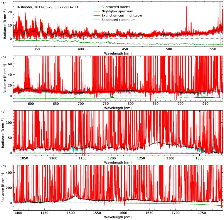
Figure 1: Extraction of nightglow continuum for an X-shooter example spectrum with an exposure time of 15 min and standard width of the entrance slit for all three arms, i.e. UVB (a), VIS (b), and NIR (c and d). Wavelengths at the margins of the arm-related spectra and beyond 1,790 nm, which are characterised by continuum data of low quality, are not shown. The green curve indicates the summed modelled contributions by scattered moonlight (not relevant here), zodiacal light, scattered starlight, and thermal emission of the telescope and instrument (multiplied by $-1$ for the plot) that were subtracted from the original sky spectrum. The cyan spectrum (or the overplotted red curve in the case of complete overlap) limited by the dotted zero line is the result of this subtraction and marks the nightglow emission. The red spectrum results from a continuum-optimised correction of the atmospheric extinction, i.e. absorption and scattering. The largest changes compared to the cyan curve are therefore related to wavelength ranges with strong absorption bands. Finally, the black solid curve shows the resulting nightglow continuum based on the application of percentile filters with wavelength-dependent percentile and width.

For the measurement of the OH line intensities in the NIR arm by noll22; noll23, lines and underlying continuum were separated by using percentile filters. For the present investigation of the nightglow continuum, we applied the same approach to the other two arms (Fig. 1). As the density and strength of emission lines depends on the wavelength, we used different combinations of percentile and window width in order to optimise the separation. Concerning the percentile, we applied a median filter in the UVB arm, a first quintile filter in the NIR arm, and stepwise transition between both limiting percentiles in the VIS arm. The window width for the major part of the spectral range was 0.8% of the central wavelength (see also noll22). This width was further modified primarily depending on the line density. In particular, extended relative widths were applied to wavelengths affected by emission bands of O_2 (e.g., noll14; noll16) at 865 nm (0.02 instead of 0.008), 1,270 nm (0.04), and 1,580 nm (0.02). Nevertheless, remnants of these bands could not be fully avoided (see Sect. 2.1).

Compared to the measurement of lines, the continuum separation was performed after two preparatory steps. First, scattered moonlight, zodiacal light, scattered starlight, and thermal emission of the telescope were calculated using the Cerro Paranal sky model (noll12; jones13) and subtracted from the X-shooter spectra (Fig. 1). Note that this is just a rough correction with relatively high systematic uncertainties, especially in the UVB arm when the Moon is up. On the other hand, the sky radiance components related to direct or scattered light of sources from outside the atmosphere are relatively weak in the NIR arm. In particular, around 1,500 nm the nightglow clearly dominates. However, the situation deteriorates beyond 1,700 nm, where the non-zero emissivity of the telescope and instrumental optical components leads to a rising thermal continuum depending on the ambient temperature. The second preparatory step was the correction of the atmospheric extinction by scattering and molecular absorption. The former was performed by means of the recipes given by noll12, which consider the change of the reference Rayleigh and Mie scattering from the sky model depending on the wavelength and zenith angle. This correction is mostly relevant for the UVB arm, where flux changes by several per cent are frequent, whereas the effect is negligible in the NIR arm. Note that the nightglow brightness even tends to increase for spectra taken close to the zenith due to Rayleigh scattering (noll12). Molecular absorption especially by water vapour but also by O_3, O_2, CO_2, and CH_4 reduces the detected radiance (e.g., smette15). Here, we also used the sky model for a correction. The continuum transmission curve was calculated for the given zenith distance, given amount of precipitable water vapour (PWV), and otherwise standard conditions at Cerro Paranal. For PWV values, we used the results from noll22 based on intensity ratios of OH lines in the NIR arm with very different absorption fractions. The applied relations were previously calibrated by means of local data from a Low Humidity And Temperature PROfiler (L-HATPRO) microwave radiometer (kerber12). Note that the simple division of a transmission curve does not provide correct results for emission lines as their natural shape is not resolved. However, as we are only interested in the continuum, we can neglect this issue here. As long as the extinction is relatively small, the results of the correction are reasonable. Nevertheless, nearly opaque wavelength regions, e.g. around 1,400 nm due to water vapour (Fig. 1), cannot be handled in this way. Even if the extinction was exactly known, small uncertainties in the flux calibration and the modelled sky radiance components would make a realistic correction impossible. Hence, the problematic wavelength regions had to be excluded from the analysis.

After the subtraction of the line emission, the continuum spectra were corrected for the increase of the emission with increasing zenith angle due to a longer geometric path through the emission layer. This van Rhijn effect (vanrhijn21) was calculated assuming that the origin of the extracted continuum was in the mesopause region. The results only weakly depend on the reference height, which we set to 90 km. The validity of the correction is supported by the consistent increase of the continuum flux with increasing zenith angle in the whole wavelength regime for the optimised sample described in Sect. 2.1.

2 Results from observations

2.1 The mean continuum

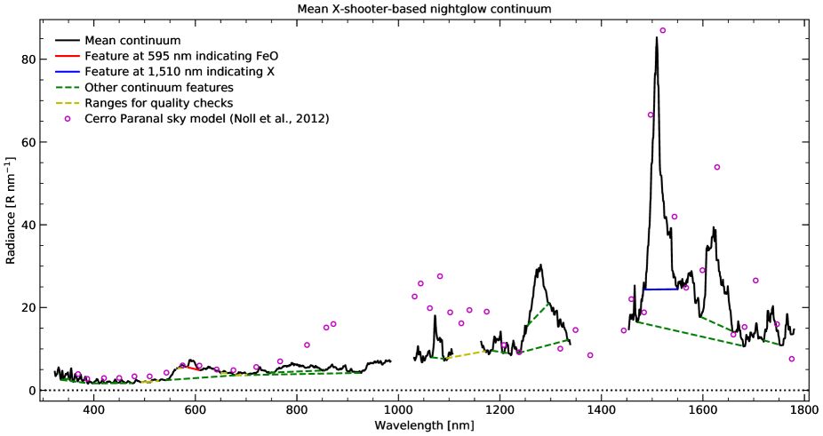
Figure 2: Mean nightglow continuum spectrum at Cerro Paranal from 10,633 combined X-shooter spectra. Wavelength ranges with systematic issues were not considered. The plot also shows the wavelength limits for different continuum features and their underlying continua that were used for the sample selection and the scientific analysis. The features centred on 595 nm (red solid line) and 1,510 nm (blue solid line) are the main structures for the latter. Other reliable continuum features (or alternative definitions of their extent) are marked by green dashed lines. The ranges indicated by yellow dashed lines were only used for quality checks (including the detection of the contamination by astronomical objects). They do not mark real nightglow features. For a comparison, the open circles show the mean residual continuum of the Cerro Paranal sky model (noll12).

For the derivation of the mean nightglow continuum and the variability of the continuum, we only selected the most reliable spectra. As a basic requirement, data products of all three arms with similar temporal coverage had to be available. In the case of arm-dependent differences in the number of exposures (e.g., by shorter exposure times in the NIR arm than in the other arms), the related spectra were averaged, weighted by the exposure time. The most important selection criterion was the minimum exposure time, which was set to 10 min after several tests. The same cut was applied to the VIS-arm sample studied by unterguggenberger17. This criterion ensures that the signal-to-noise ratio is high. However, the most important effect is the reduction of continuum contamination by bright astronomical sources, which tend to be observed with short exposure times. In order to keep the non-nightglow sky radiance (and the uncertainties of its correction) low, observations with the Moon above the horizon and an illumination of more than 50% were excluded. In the end, these criteria led to 12,723 combined spectra, which constitutes a substantial decrease compared to the full sample. In a second selection procedure, various features in the continuum probably belonging to the nightglow continuum, residuals of nightglow lines, or residuals of astronomical objects (e.g. the H$\alpha$ line), and the remaining underlying continuum were measured to identify spectra with suspected artefactual contamination (Fig. 2). The resulting selection limits (e.g. non-negative continuum fluxes), which were validated by visual inspection of spectra with values close to the limits, led to a sample of 10,850 spectra. In a third step, the selection was further refined by the search for abrupt changes in the times series of the continuum flux due to the change of the astronomical target, which suggests a residual contamination. Also validated by visual inspection, this procedure resulted in a final sample of 10,633 combined spectra.

The mean of this data set is shown in Fig. 2. The spectrum has gaps in wavelength ranges at the margins of the arms (due to high systematic uncertainties) and strong atmospheric absorption (essentially by water vapour). The latter explains the spectral upper limit at 1,780 nm, which also avoids wavelengths with strong thermal emission of the telescope (Fig. 1). At short wavelengths (i.e. in the UVB arm), various bands related to the electronic upper states c, A^′, and A of O_2 (e.g., slanger03; cosby06) are visible. As the bands are only partially resolved in the X-shooter spectra, the major portion of the emission appears to be present as continuum.

The pronounced step in the continuum at about 555 nm and the peak at about 595 nm indicates the presence of emission from the FeO orange bands (west75; jenniskens00; burgard06; evans10; saran11; gattinger11a; unterguggenberger17). The location of the step does not support significant contributions by NiO (burgard06; evans11; gattinger11b), at least from the bluest systems (B-X and C-X), which would already lead to a rise of the flux below 500 nm. The shape of the continuum in this wavelength range also excludes a significant contribution of NO_2 air afterglow (becker72; gattinger09; gattinger10; semenov14a), which is not unexpected as it is usually only bright at high latitudes (see also Sect. Structure, variability, and origin of the low-latitude nightglow continuum between 300 and 1,800 nm: Evidence for HO_2 emission in the near-infrared). Longwards of the peak at 595 nm, the continuum shows only minor features in the VIS arm with a shallow local maximum at about 800 nm. There, the flux level is not higher than around the FeO main peak and lower than all published continuum measurements in this wavelength range (Sect. Structure, variability, and origin of the low-latitude nightglow continuum between 300 and 1,800 nm: Evidence for HO_2 emission in the near-infrared). At 857 nm, where noxon78 obtained a relatively low value of about 7 R nm^-1, our mean flux is about 5.0 R nm^-1. For a comparison, Fig. 2 also shows the mean continuum from the Cerro Paranal sky model of noll12. While up to 770 nm the model continuum is usually only slightly brighter than our X-shooter-based measurements, the subsequent three data points are above 10 R nm^-1, which was most probably caused by the use of spectra without sufficient resolving power.

In the NIR arm, our mean continuum is highly structured. In part, these features are related to residuals of blends of strong OH and O_2 nightglow emission lines. In particular, remnants of the O_2 bands at 1,270 and 1,580 nm related to the transitions (a-X)(0-0) and (a-X)(0-1) can be identified (e.g., rousselot00; noll14; noll16). Nevertheless, these features only include a very small fraction of the total emissions, which were separated with particularly wide filter windows because of the relatively high line density (see Sect. 1.2). The feature at about 1,080 nm is probably mainly related to the weak O_2(a-X)(1-0) band (HITRAN database; gordon22), although the narrow maximum appears to be affected by OH residuals. The most striking continuum feature is certainly the high and narrow peak at about 1,510 nm. It is not related to residuals of strong lines. Hence, it is probably composed of a high number of weak lines, which cannot be resolved with the spectral resolving power of X-shooter. A feature with a similar origin appears to be the peak at about 1,620 nm.

Both features do not appear to have been discussed previously in the airglow literature. Nevertheless, they are already indicated in the coarse residual continuum component of the Cerro Paranal sky model (noll12), which was also derived from X-shooter spectra (see Sect. Structure, variability, and origin of the low-latitude nightglow continuum between 300 and 1,800 nm: Evidence for HO_2 emission in the near-infrared). Despite the high uncertainties in the model due to premature processing of only a small number of spectra, the majority of the measurement points are relatively close to our mean continuum. Notable exceptions in the NIR-arm range are the fluxes at 1,628 nm (54 R nm^-1) and below 1,180 nm. Apart from possible problems with the separation of lines and continuum, the offsets in the latter range suggest systematic issues with the data processing. Data points in ranges that we excluded from our analysis should be treated with caution. In Australia, trinh13 coincidentally performed their continuum measurement of $30\pm 6$ R nm^-1 near the emission peak between 1,516 to 1,522 nm. We find a higher flux of about 50 R nm^-1 for the same range. On the other hand, the mean continuum between 1,661 and 1,669 nm in Fig. 2 amounts to about 14 R nm^-1, which is clearly lower than the measurements of maihara93 and sullivan12. However, it is slightly brighter than a radiance of about 11 R nm^-1 proposed by oliva15 after the correction of the flux of maihara93 for the contamination by faint OH lines. Compared with the mean continuum flux of about 16 R nm^-1 obtained by oliva15 between 1,519 to 1,761 nm with high resolving power, our corresponding flux of about 22 R nm^-1 is also slightly higher. Apart from differences in the instrumental properties and the data processing, such discrepancies could also be explained by the different observing sites and observing periods. oliva15 only used 2 h of data taken at La Palma (29^∘ N).

2.2 Continuum decomposition

Most of the nightglow continuum emission in Fig. 2 does not exhibit clear features. In order to better understand this emission and its relation to the identified features, we performed a decomposition of the continuum in different components by means of the wavelength-dependent variability pattern derived from the 10,633 selected spectra. Our approach was to use non-negative matrix factorisation (NMF; e.g., lee99; noll23) as it is well suited for additive components without negative values. NMF approximately decomposes an $m\times n$ matrix $\mathbf{X}$ without negative elements into two non-negative matrices $\mathbf{A}$ and $\mathbf{B}$ with sizes $m\times L$ and $L\times n$, respectively, by usually minimising the squared Frobenius norm of $\mathbf{X}-\mathbf{A}\mathbf{B}$. For this analysis, $m$, $n$, and $L$ are the number of wavelength positions, number of spectra, and number of continuum components, respectively. As we sampled the continuum spectrum with a resolution of 0.5 nm and only included the ranges indicated in Fig. 2, $m$ was 2,479. For $L$, a reasonable minimum is 4 since the features correlated with the FeO emission in the VIS arm, the unidentified features in the NIR arm, the O_2 features in the UVB arm, and the residuals related to the O_2(a-X) bands in the NIR arm should be treated separately. This definition of basic variability classes is supported by a check of the correlations between the variability of the different measured features and continuum windows. In the following, we call these classes FeO(VIS), X(NIR), O_2(UVB), and O_2(NIR). The names refer to the radiating molecule and location (in terms of the X-shooter arm) of the main features of each class. It is not excluded that emission of other molecules with a similar variability pattern can contribute. For the application of the NMF, negative fluxes have to be avoided. Because of the thorough sample selection procedure described above, the number of affected data points was very small and negative values could therefore be replaced by zeros without a significant change of the mean spectrum. Only between 1,031 and 1,037 nm (the shortest considered wavelengths in the NIR arm), the mean flux increased by more than 1%. For the derivation of the mean spectrum of each component, we multiplied each of the resulting $L$ component spectra consisting of $m$ data points with the mean of the $n$ corresponding scaling factors.

In the case of an application of the NMF with $L=4$, it turned out that the O_2 component in the UVB arm was not separated from the FeO-related features (similar to $L=3$). This failure was probably caused by the weakness of the O_2 features compared to the other identified continuum structures. As a consequence, we increased the weight of wavelength regions where a crucial feature was relatively strong by the multiplication of suitable factors before the NMF and the division of the same factors in the resulting component spectra. Consequently, the algorithm minimised $\left|\left|\mathbf{X^{\prime}}-\mathbf{A^{\prime}}\mathbf{B}\right|\right|^{2}_{\mathrm{Fro}}$, where $\mathbf{X^{\prime}}=\mathbf{S}\mathbf{X}$ and $\mathbf{A}=\mathbf{S}^{-1}\mathbf{A^{\prime}}$ with $\mathbf{S}$ being a diagonal $m\times m$ matrix containing the wavelength-dependent scaling factors. We tested different numbers and sizes of the windows. In the end, we used 335 to 359 nm, 586 to 603 nm, 1,260 to 1,297 nm, and 1,497 to 1,521 nm, which maximised the weight of the main features of the four variability classes. To find the best scaling factors, we defined a cost function $C$ that uses the relative contributions $f_{ij}$ of the $L=4$ component spectra to the four corresponding feature windows as defined above, i.e. we attempted to minimise $C=1-\sum^{L}_{i=1}w_{i,\mathrm{max}}\,f_{i,\mathrm{max}}$, where $w_{i,\mathrm{max}}$ and $f_{i,\mathrm{max}}$ being the weight and relative flux of the most relevant feature window $j$ contributing to component $i$. Equal weights of 0.25 for the four feature windows favoured solutions with particularly large contributions of the two O_2-related components. However, the latter can be seen as contaminations of the FeO(VIS) and X(NIR) components, which are obviously the primary targets of an investigation of the nightglow continuum. Hence, we added the fractions with different weights, finally choosing 0.33 for FeO(VIS) and X(NIR) and 0.17 for O_2(UVB) and O_2(NIR). This (somewhat arbitrary but non-critical) definition was sufficient to easily distinguish between solutions with good component separation (best $C$ of 0.26) and those where the separation failed, especially in the case of O_2(UVB) and FeO(VIS) (best $C$ of 0.32). The relation between the scaling factors in $\mathbf{S}$ and the structure of the component spectra turned out to be complex. However, the variations within a certain class of solutions tended to be relatively small. Hence, the solutions related to a satisfactory separation of the four components as indicated by low $C$ are relatively robust. In any case, there are two major components that dominate the visual and near-infrared ranges.

In order to find minima of the cost function, we applied a simplicial homology global optimisation (SHGO; endres18) algorithm in the “sobol” mode with 512 sampling points and a limitation of the scaling factors between 1 and 200. The resulting list of local minima for $L=4$ suggests an uncertainty in the contribution fractions of several per cent for the windows in the UVB and VIS arm and close to 1% for the two windows in the NIR arm. Eventually, we fine-tuned the most promising solution with scaling factors of about 139, 96, 68, and 65 (listed with increasing central wavelength of the feature window) by starting an unconstrained simplex search algorithm (nelder65) with the given values as initial parameters. The resulting factors were about 1291, 865, 638, and 597, which differ from the initial values only by a nearly constant factor. This points to a degeneracy of solutions, related to the fact that the values are much higher than 1, i.e. the NMF results appear to be mostly determined by the narrow feature windows. All reasonable local minima found by SHGO in the parameter space are characterised by relatively high values (limited to a maximum of 200), although the ratios of the four factors can clearly differ.

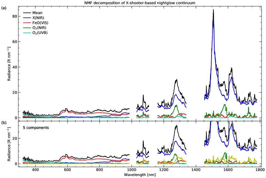
Figure 3: Decomposition of mean nightglow continuum spectrum at Cerro Paranal (black curve) into (a) four and (b) five components by non-negative matrix factorisation of the selected 10,633 X-shooter spectra. The details of the procedure are discussed in Sect. 2.2. The four main components are labelled X(NIR), FeO(VIS), O_2(NIR), and O_2(UVB), which indicates the emitting molecule (if known) and the X-shooter arm with the dominating contribution. The fifth component in (b) appears to mainly consist of residuals of strong nightglow emission lines.

The resulting mean continuum components based on refined simplex search are shown in Fig. 3a. The FeO(VIS) and X(NIR) components contribute to the corresponding feature windows with 83.0% and 95.1%, respectively. Other reasonable solutions tend to show slightly lower percentages. The dominance of these two components extends to wavelengths far away from the main features. While FeO(VIS) dominates almost the entire VIS arm, X(NIR) is the strongest mean component in the NIR arm. Similar contributions appear to be present at the red end of the VIS arm. Below 500 nm, O_2(UVB) becomes important with a dominating contribution of 60.5% in the reference range between 335 and 359 nm. Nevertheless, FeO(VIS) appears to still contribute with non-negligible 25.0% there. In terms of the interpretation of this emission as based on FeO, this result is questionable as Reaction Structure, variability, and origin of the low-latitude nightglow continuum between 300 and 1,800 nm: Evidence for HO_2 emission in the near-infrared should only be exothermic by about 300 kJ mol^-1 (helmer94), which corresponds to a minimum wavelength of about 400 nm. Although the separation of O_2(UVB) and FeO(VIS) shortwards of the FeO main peak seems to be the most uncertain result of the NMF-based continuum decomposition, the FeO(VIS) contributions in the UVB arm might support the presence of the blue FeO bands described by west75. With a higher significance, the high contribution of the component at about 800 nm might be explained by the presence of the FeO IR bands (bass52; west75), although the emission looks smoother than in the laboratory, where it was not produced by Reaction Structure, variability, and origin of the low-latitude nightglow continuum between 300 and 1,800 nm: Evidence for HO_2 emission in the near-infrared. According to the analysis of gattinger11a, the emission of the FeO orange bands is also less structured in the mesopause region than in the laboratory due to a wider distribution of the vibrational populations. Moreover, it is possible that residuals of other emissions in the X-shooter continuum spectra led to an excessive removal of small-scale features. The direct measurement of the broad feature between 745 and 855 nm (Fig. 2) at least shows that the strength of this structure is well correlated with the peak at 595 nm. The measurements in the laboratory found FeO emission up to 1,400 nm. The FeO(VIS) spectrum appears to show a similar extension. However, the uncertainties of the minor contributions in the NIR arm compared to X(NIR) are large.

The FeO(VIS) component could partly be produced by other metal-bearing molecules if their emission showed a similar emission pattern. As already discussed in Sect. 2.1, NiO would be a candidate but the shape of the continuum between 500 and 600 nm does not seem to allow a major contribution. We searched for other possible molecules that could produce a pseudo-continuum in the investigated wavelength regime. A survey of the metal-related chemistry in the mesopause region turned out that another abundant Fe-containing reservoir species (plane03; feng13; plane15) could be a possible candidate. Unfortunately, chemiluminescence spectra of these molecules do not appear to exist. Nevertheless, inspection of the energetics of the relevant chemical reactions only left the reaction FeOH + O