The Kepler Cone, Maclaurin Duality and Jacobi-Maupertuis metrics.

Abstract.

The Kepler problem is the special case $\alpha=1$ of the power law problem: to solve Newton’s equations for a central force whose potential is of the form $-\mu/r^{\alpha}$ where $\mu$ is a coupling constant. Associated to such a problem is a two-dimensional cone with cone angle $2\pi c$ with $c=1-\frac{\alpha}{2}$. We construct a transformation taking the geodesics of this cone to the zero energy solutions of the $\alpha$-power law problem. The ‘Kepler Cone’ is the cone associated to the Kepler problem. This zero-energy cone transformation is a special case of a transformation discovered by Maclaurin in the 1740s transforming the $\alpha$- power law problem for any energies to a ‘Maclaurin dual’ $\gamma$-power law problem where $\gamma=\frac{2\alpha}{2-\alpha}$ and which, in the process, mixes up the energy of one problem with the coupling constant of the other. We derive Maclaurin duality using the Jacobi-Maupertuis metric reformulation of mechanics. We then use the conical metric to explain properties of Rutherford-type scattering off power law potentials at positive energies. The one possibly new result in the paper concerns “star-burst curves” which arise as limits of families negative energy solutions as their angular momentum tends to zero. We also describe some history around Maclaurin duality and give two derivations of the Jacobi-Maupertuis metric reformulation of classical mechanics. The piece is expository, aimed at an upper-division undergraduate. Think American Math. Monthly.

1. The Kepler Cone

Take a sheet of paper. Join adjacent corners, creasing and folding so as to bisect their common edge. Join the resulting two half-edges together and tape together. You have formed part of the Kepler cone with the old edge forming one generator. Lines drawn on the paper become geodesics on the cone. See figure 1. The cone embeds isometrically in 3-space as the locus

$$x^{2}+y^{2}=3z^{2},z\geq 0.$$

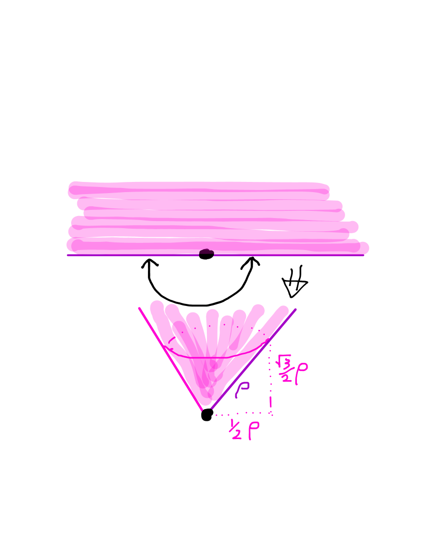
Figure 1. Folding a sheet of paper to make a cone.

Place the Kepler cone off to the side. Take out a new sheet of paper representing a Euclidean plane which we call the Newtonian plane. Mark an origin on this plane. Draw some parabolas on the plane with origin as focus. When parameterized according to Kepler’s second law (“equal times in equal areas”) these parabolas are the zero-energy solutions to Kepler’s problem

(1) $$\ddot{q}=-\mu\frac{q}{r^{3}},r=\|q\|:=\sqrt{x^{2}+y^{2}}.$$

Here $\mu$ is a positive constant called the “coupling constant”. The vector $q=(x,y)\in\mathbb{R}^{2}$ coordinatizes the Newtonian plane. A solution to Kepler’s problem is a curve $t\mapsto q(t)$ parameterized by Newtonian time $t$. Dots over $q$ denote time derivatives so that in the equation $\ddot{q}$ denotes the acceleration or second derivative. And $\dot{q}$ denotes the velocity or first derivative along the curve. The energy associated to Kepler’s problem is

(2) $$E=\frac{1}{2}|\dot{q}|^{2}-\frac{\mu}{r}.$$

and is constant along solutions to equation (1). The Kepler parabolas, and their degenerations, the rays through the origin, exhaust the supply of zero energy solutions to Kepler’s problem.

Retrieve the Kepler cone. Consider the plane containing the sheet of paper used to make the cone. Call this the folding plane. Put Cartesian coordinates $Q=(u,v)$ on the folding plane so that the origin $O$ is the midpoint of the edge of the sheet paper and the sheet lies in the half-plane $v\geq 0$. When we fold and glue we identify points along the bounding line $v=0$ by the isometry $Q\mapsto-Q$. The two rays merge to form a single generator of the Kepler cone which we will call the seam. Rotate the half-plane and we get another representation of the Kepler cone, one with a different seam. When we use this new half-plane the gluing map still glues $Q$ to $-Q$ on its bounding line. If $Q$ is in the interior of the half-plane then $-Q$ is in the complement of the closed half-plane. We have derived the following algebraic construction of the Kepler cone.

Lemma 1.

The Kepler cone is the metric quotient $\mathbb{R}^{2}/(\pm 1)$ of $\mathbb{R}^{2}$ by the action of the two element group $\pm 1$ acting by $Q\mapsto\pm Q$.

We describe in subsection 6.1 what we mean by “metric quotients”, that is to say, how the Euclidean metric on $\mathbb{R}^{2}$ induces a metric on the quotient.

Identify the folding plane and the Newtonian plane with a copy of $\mathbb{C}$ by writing $q=(x,y)=x+iy$ and $Q=(u,v)=u+iv$. Then squaring

(3) $$Q\mapsto q=Q^{2},$$

defines a map from the folding plane to the Newtonian plane. Because $(-Q)^{2}=Q^{2}$, the squaring map induces a map from the Kepler cone to the Kepler plane, namely the map $\{Q,-Q\}\to Q^{2}$.

Exercise 1.

Show that squaring (3) takes straight lines to Kepler parabolas.

Did foisting this exercise on you feel like pulling a rabbit out of a hat? Sure, you can do the algebra, but why should it be true?

Introduce the “Jacobi-Maupertuis” metric

$$ds^{2}_{1}=\frac{4|dq|^{2}}{|q|}\text{ where }|dq|^{2}=dx^{2}+dy^{2}$$

on the Kepler plane. This metric is Riemannian away from $q=0$ and the distance function which it induces on the Newtonian plane is that of a complete metric space.

Proposition 1.

A. The Kepler parabolas are geodesics for the metric $d^{2}s_{1}$.

B. Squaring (map (3)) induces an isometry between the Kepler cone and the Kepler plane endowed with the Jacobi-Maupertuis metric $ds^{2}_{1}$.

Recall that the straight lines in the folding plane became geodesics on the cone. Since isometries take geodesics to geodesics, the proposition supplies a metric explanation of our rabbit out of the hat trick.

Proposition 1 generalizes to other cones and other force laws. A choice of smooth function $V:\mathbb{R}^{2}\to\mathbb{R}$ defines a Newton’s equations:

(4) $$\ddot{q}=-\nabla V(q).$$

These equations admit a conserved energy

$$E(q,v)=K(v)+V(q),\qquad K(v)=\frac{1}{2}|v|^{2},v=\dot{q}$$

as did Kepler’s problem whose potential is $V=-\mu/r$.

By a central force problem we mean Newton’s equations (4) for a rotationally symmetric potential: $V(q)=f(r)$ where $r=\|q\|$ for some $f:\mathbb{R}_{+}\to\mathbb{R}$. We are concerned here with central force problems of the form $V(q)=-\mu/r^{\alpha}$. We call these power law potentials and the corresponding Newton’s equations (equation (10) below) the power law problem or power law dynamics.

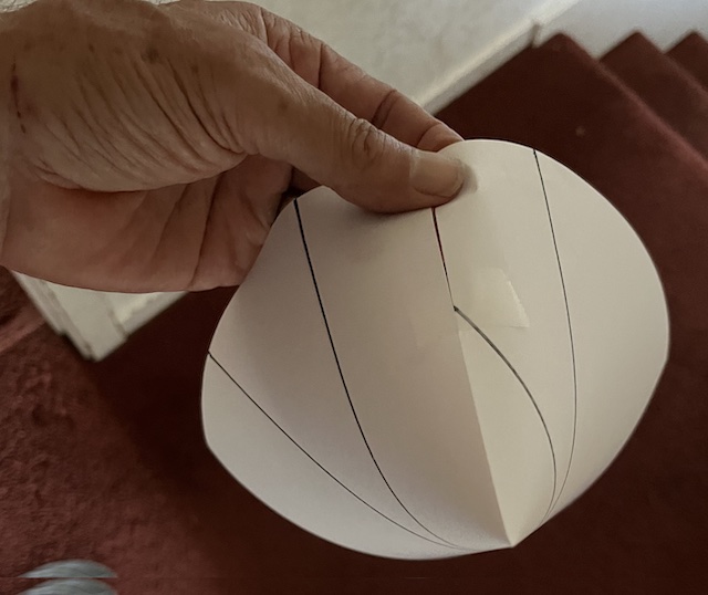
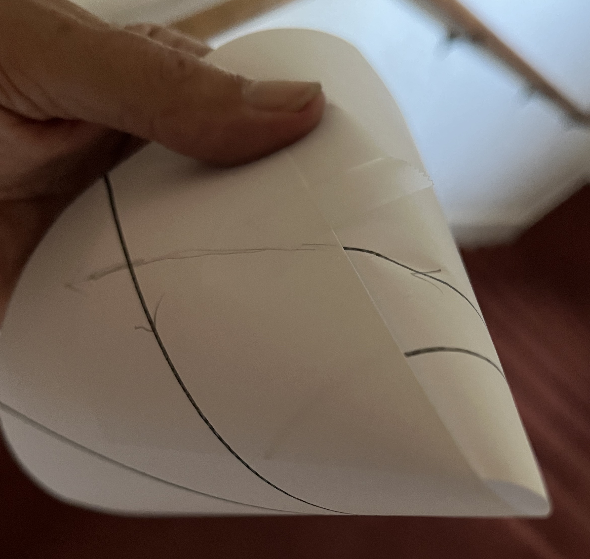
Figure 2. Sharpening the cone angle.

Theorem 1.

A. The geodesics for the JM [Jacobi-Maupertuis] metric

(5) $$ds^{2}_{\alpha}=\frac{|dq|^{2}}{|q|^{\alpha}}$$

are the zero energy solutions to the power law problem (equation (10)).

B. The JM metric (5) is isometric to the conical metric

(6) $$ds^{2}_{cone}=d\rho^{2}+c^{2}\rho^{2}d\theta^{2},\text{ with }c=1-\frac{\alpha}{2}$$

provided $\alpha\neq 2$. This is the metric for a two-dimensional cone of angle $|c|$. Here $(\rho,\theta)$ are polar coordinates on the plane and are related to the polar coordinates $(r,\theta)$ of $q=re^{i\theta}$ of the Newtonian plane by $\rho=r^{c}$.

C. Again with $\alpha\neq 2$, the map $Q\mapsto q=Q^{1/c}$ maps straight lines on the folding plane and hence geodesics on the cone of part B, to the zero energy solutions to Newton’s equations described in part A.

Remark on Part B The coordinates $(\rho,\theta)$ of part B are related to the folding coordinate $Q\in\mathbb{C}$ of part C as follows. Write $Q=\rho e^{i\psi}$. Then $\theta=\frac{1}{c}\psi$. For example, for the Kepler cone $\theta=2\psi$ and the metric of B is $d\rho^{2}+\frac{1}{4}\rho^{2}d\theta^{2}$. See section 5 for more on cones and for a proof of part B.

Remark on $\alpha=2$. When $\alpha=2$ the JM metric is isometric to that of a cylinder, not a cone. See subsection 5.3 below.

On folding these cones We can make all the cones of the theorem having $1\leq\alpha<2$, so $0<c\leq 1/2$, from the same sheet of paper out of which we made the Kepler cone. Take the two half-edges that we had earlier glued as soon as they had touched and continue to wrap them around tighter so as to make the cone tighter and sharper before taping the half-edges down. Lines drawn on the paper still make geodesics on the cone. Sharper cones means larger coefficients $A^{2}$ in the equation of the cone. See figure 2.

Alternatively, here is a paper folding construction that works for all $0<\alpha<2$. Cut a sector out of the folding plane, whose opening angle is $2\pi(1-c)$ where $c=1/\beta$, leaving a sector whose opening angle is $2\pi c$. Glue the two rays bounding this remaining sector together to make any of the cones of part B of the proposition. (We discuss cones in detail further on.)

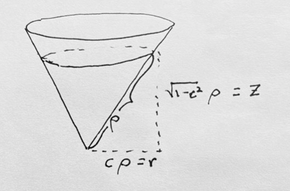
Figure 3. The metric on the cone of part B can be emdedded as a cone of revolution in three-space provided $0<c<1$.

These cones embed as cones of revolution in $\mathbb{R}^{3}$ provided $0<c<1$. See figure 3. Some algebra shows that the cone is described as

$$x^{2}+y^{2}=Az^{2},z\geq 0\text{ with }A=\frac{1-c^{2}}{c^{2}}.$$

Here $\rho^{2}=x^{2}+y^{2}+z^{2}$ and $r^{2}=x^{2}+y^{2}$.

The Jacobi-Maupertuis principle, presented in the next section, provides the engine behind Theorem 1 and its corollary, Proposition 1.

2. Jacobi-Maupertuis

Return to Newton’s equations (4). Allow the potential $V$ to have poles, i.e. to take on the values $\pm\infty$. We will also call the poles “collision points”, in honor of the Kepler problem where $V(q)=-\infty\iff q=0$. In the Kepler problem $q$ records the planet’s location and the origin represents the sun location so that $q=0$ means that the planet has collided with the sun. We assume $V$ to be continuous everywhere and smooth away from collision points.

Recall that the total energy $E(q,v)=K(v)+V(q)$ is conserved. From $K(v)\geq 0$ we see that if a solution $q(t)$ has energy $E$ then along the solution $V(q(t))\leq E$. In other words, solutions having energy $E$ are constrained to lie in the region $\{q\in\mathbb{E}:E\geq V(q)\}$ within the Newtonian plane. We call this region the “Hill region” for the choice of energy $E$ and its boundary $\{q\in\mathbb{R}^{2}:E=V(q)\}$ we call the Hill boundary.

Definition 1.

The Jacobi-Maupertuis [JM for short] metric at energy $E$ for the Newton’s equation (4) is the Riemannian metric

(7) $$ds^{2}_{JM}=2(E-V(q))|dq|^{2}$$

defined on the Hill region $\{V\leq E\}$ and degenerating at its boundary $\{V=E\}$.

We say that $q_{0}=q(t_{0})$ is a brake point of a solution $q(t)$ if $\dot{q}(t_{0})=0$. The solution has “braked” to a stop. If the energy of this solution $E$ then being a brake point is equivalent to hitting the Hill boundary since then $V(q)=E$ if and only if $K(\dot{q}(t))=0$.

Theorem 2 (Jacobi-Maupertuis principle).

Away from collisions and brake points, every energy $E$ solution to Newton’s equations is the reparameterization of a geodesic for the energy $E$ JM metric (7) on the Hill region. Conversely, away from collisions and the Hill boundary, every JM geodesic is a reparameterization of an energy $E$ solution of Newton’s equations.

See section 8 for proofs of the theorem.

Proof of part A of proposition 1. Newton showed that the non-collision solutions to Kepler’s problem satisfy Kepler’s 1st law: they are conic sections with one focus at the origin. He also showed that the zero energy solutions are the parabolas. Part A of the proposition now follows immediately from the theorem.

3. Squaring and Levi-Civita

Take the JM metric for Kepler’s problem at any energy:

$$ds^{2}=2(E+\frac{\mu}{r})|dq|^{2}$$

The squaring substitution $q=Q^{2}$ yields $r=|q|=|Q|^{2}$, $dq=2QdQ$ and $|dq|^{2}=4|Q|^{2}|dQ|^{2}$. Then $\frac{1}{r}|dq|^{2}=4|dQ|^{2}$. The singularity of the metric at the origin $r=0$ has cancelled out! Rewritten in terms of $Q$ we find

$$ds^{2}=2(4E|Q|^{2}+4\mu)|dQ|^{2}$$

We recognize this to be the JM metric at energy $4\mu$ associated with the potential energy $W(Q)=-4E|Q|^{2}$ on the folding plane. In going from $V=-\mu/r$ to $W$ the roles of the energy $E$ and coupling constant $\mu$ have switched! The corresponding Newton’s equations on the folding plane are the linear equations

(8) $$Q^{\prime\prime}=8EQ$$

where the second derivative $Q^{\prime\prime}$ is with respect to a ‘Newtonian time” $\tau$ on the folding plane. It follows that the squaring transformation maps solutions of the linear equation (8) to solutions to Kepler’s equations having energy $E$.

Proof of part B of proposition 1. When $E=0$ we have that $ds^{2}=4\mu|dQ|^{2}$, which is the flat metric on the folding plane. Upon folding this metric in turn induces the metric on the Kepler cone upon folding. The linear ODE (8) is that of a straight line $Q^{\prime\prime}=0$ which fold to geodesics on the cone. Remarks on scaling. Multiplying a metric by a positive constant does not change its geodesics, so we could just as well use $|dQ|^{2}$ instead of $4\mu|dQ|^{2}$ and correspondingly dilated the Kepler cone metric. Cones, like the Kepler cone, admits dilations. However we scale the metric on the Kepler cone , the circle of radius $\rho$ about the cone point will have circumference $\pi\rho$, not $2\pi\rho$. Scaling the folding plane by $\lambda$ effects scaling its quotient, the Kepler cone, by $\lambda$

We return to the question of the time $\tau$ used in taking the second derivative defining the ODE (8) in the folding plane, deduced now for general energies $E$ in the Newtonian plane. What is the relation between Newtonian time $t$ and this other time $\tau$? If $s$ is JM arclength then we have

$$\frac{d\tau}{dt}=\frac{d\tau}{ds}\frac{ds}{dt}.$$

Recall the relation $ds=\lambda dt$ between JM arc-length $s$ and Newtonian time $t$ when we use the JM principle and where $\lambda=2(E+V(q))$ is the conformal factor relating the Euclidean metric and the JM metric. On the $q$ plane with its time $t$ we have $\lambda=2(E+\mu/r)$ so $\frac{ds}{dt}=2(E+\mu/r)$. But on the $Q$ plane with its time $\tau$ and potential $W(Q)=-4E|Q|^{2}=-4Er$ we have $ds=\tilde{\lambda}d\tau$ with $\tilde{\lambda}=2(4Er+4\mu)=4r(2E+\mu/r)$ and so $\frac{d\tau}{ds}=\frac{1}{4r(2E+\mu/r)}$. It follows that $d\tau/dt=1/4r$ or

(9) $$d\tau=\frac{dt}{4|q|}$$

The Levi-Civita transformation is the squaring map (3) together with the time reparameterization (9). See section 4 regarding the long history of an old generalization of this transformation and its name. We have shown that this transformation has the remarkable property that it takes solutions to Kepler’s problem to solution to the linear “oscillator” equation (8).

3.1. Maclaurin Duality for power law problems.

The Levi-Civita transformation exhibits a duality between the Kepler force law generated by the $1/r$ gravitational potential and the linear force law of Hooke generated by an $r^{2}$ potential. Maclaurin knew of this duality centuries before Levi-Civita, having had discovered a generalization which applies to any power law problem. The $\alpha$ power law problem, namely Newton’s equations for the power law potential $V=-\mu r^{-\alpha}$, is

(10) $$\ddot{q}=-\mu\alpha\frac{q}{|q|^{\alpha+2}}.$$

The associated JM metric at energy $E$ for this $V$ is

$$ds^{2}=2(E+\mu/r^{\alpha})|dq|^{2}.$$

The substitution $q=Q^{\beta}$ yields $dq=\beta Q^{\beta-1}dQ$ and $r=|Q|^{\beta}$. The trick is to tune the exponent $\beta$ so that the factor $|Q|^{2(\beta-1)}$ occuring in the identity $|dq|^{2}=\beta^{2}|Q|^{2(\beta-1)}|dQ|^{2}$ cancels with the factor $\frac{1}{r^{\alpha}}$ arising from the singularity of the potential. Thus we require $2(\beta-1)=\beta\alpha$ or

(11) $$2-\frac{2}{\beta}=\alpha\text{ or }\beta=\frac{2}{2-\alpha}$$

With this choice of $\beta$ we find that, written out in the $Q$-variable,

(12) $$ds^{2}=2(\beta^{2}E|Q|^{\gamma}+\mu\beta^{2})|dQ|^{2}$$

where

(13) $$\gamma=2\beta-2=\frac{2\alpha}{2-\alpha}$$

We recognize expression (12) as the JM metric in the folding plane for energy $\mu\beta^{2}$ associated to the power law potential $W(Q)=-\beta^{2}E|Q|^{\gamma}$. Its corresponding Newton’s equation is

(14) $$Q^{\prime\prime}=\frac{E\gamma}{\mu\alpha}|Q|^{\gamma-2}Q.$$

This transformed ODE is the “Maclaurin dual” to our original power law problem, equation (10).

The transformed ODE (14) is a differential equation for curves $Q=Q(\tau)$ in the folding plane. The new time $\tau$ of $Q^{\prime\prime}=\frac{d^{2}Q}{d\tau^{2}}$ is not the old Newtonian time $t$ used for the $q$-equation. The same trick we used when we derived the reparameterization part of the Levi-Civita transformation works here to find the relation between the $t$-time of the Newtonian plane and the $\tau$-time of the folding plane. This trick used the JM arclength $s$ as an intermediary between the two times. We have

(15) $$\frac{d\tau}{dt} = \frac{d\tau}{ds}\frac{ds}{dt}$$

(16) $$= (2(E\beta^{2}|Q|^{\gamma}+\mu\beta^{2}))^{-1}2(E+\mu/r^{\alpha})$$

Now factor out $\beta^{2}|Q|^{\gamma}$ from the first denominator $2(E\beta^{2}|Q|^{\gamma}+\mu\beta^{2})$, recalling that we tuned $\beta$ so that $|Q|^{-\gamma}=r^{-\alpha}$. We get that $2(E\beta^{2}|Q|^{\gamma}+\mu\beta^{2})=\beta^{2}r^{\alpha}(2(E+\mu/r^{\alpha})$. It follows that

$$\frac{d\tau}{dt}=\frac{1}{\beta^{2}r^{\alpha}}$$

We summarize. Let the exponents $\alpha,\beta,\gamma$ be related by the relations (11, 13). We could equivalently summarize the relations by

(17) $$(1-\frac{\alpha}{2})(1+\frac{\gamma}{2})=1,\qquad\frac{\alpha}{2}+\frac{1}{\beta}=1$$

Then the transformation

(18) $$q=Q^{\beta},dt=\beta^{2}|q|^{\alpha}d\tau$$

takes solutions $q(t)$ to (14 ) having energy $E$ to solutions $Q(\tau)$ to the ODE (14 ). We will call the transformation ( 18) the “Maclaurin transformation” in honor of Maclaurin who discovered this duality between central force laws whose exponents $-\alpha,+\gamma$ are related by (17). See [16] section 451 for the statement and section 875 for the proof.

Multivalued maps.

$Q\mapsto Q^{\beta}$ is a multivalued map when $\beta$ is not an integer, so some care must be taken in applying the transformation. We can proceed as follows. Let $Q=\rho e^{i\psi}$. Then the values taken by $Q^{\beta}$ are any one of the possibly countably many values $q=\rho^{\beta}e^{i(\beta\psi+2\pi\beta k)}$, $k\in\mathbb{Z}$. Let $Q(\tau),\tau\in\mathbb{R}$ be an analytic curve in the plane which misses the origin. Choose a point, say $Q(0)$ along this curve and one of these values, $q_{0}$ for $Q(0)^{\beta}$. Analytically continue $Q^{\beta}$ along the entire curve. In this way we construct an image curve $q(\tau)=Q^{\beta}(\tau)$ passing through $q_{0}$. Reparameterize $q(\tau)$ by $t$ by doing the integral defining the relation between $t$ and $\tau$ so as to get the Maclaurin transformed curve $q(t)$. Different choices of initial value for $q_{0}$ will be related by rotation by some angle $2\pi\beta k$. The corresponding transformed curve through this new $q_{0}$ will be related to the original curve by this same rotation. It is still a solution since rotations act as symmetries of central force problems.

The inverse process is identical. Start with a curve $q(t)$ and choose a branch of $q\mapsto q^{1/\beta}=Q$ near $q(0)$ and analytically continue $q^{1/\beta}$ along $q(t)$. We have a unique analytic continuation as long as the curve $q(t)$ misses the origin. Then we can reparameterize it to get a curve $Q(\tau)$. In this way we have a correspondence between the non-collision solutions to the two ODEs.

It is worth remarking that the collision solutions, being rays through the origin also correspond to each other under the Maclaurin transformation.

4. An Abbreviated History of Maclaurin’s duality.

In an early draft of this article I used “Bohlin transformation” for what I now call the “Maclaurin transformation”, the transformation which yields what I’m calling Maclaurin duality. Arnol’d used “Bohlin transformation” in his book [3], which is where I learned about this remarkable duality. I sent this early draft to Alain Albouy who corrected my historical misunderstandings. I copy some of the history which Albouy and Zhang [1] have unearthed, restating it in an abbreviated form.

1742. Colin Maclaurin [16], in section 451 of his Treatise of fluxions, states the duality of the previous section, proving it in section 875.

1889. Goursat [11] rediscovers Maclaurin duality using the Hamilton-Jacobi equation and conformal maps.

1889. Darboux [8] extends Goursat [11] to mechanics in curved, multidimensional spaces.

1894. Painlevé [18], inspired by Darboux, asks in [18]. He “what are all the transformations which, together with time reparameterizations, send one system onto another?” He analyzes previous works on page 17 of this publication.

1896. Painlevé [19] answers his question for two degrees of freedom systems. Darboux’s examples, and so Maclaurin duality, are one of Painlevé’s main cases.

1900. Ricci and Levi-Civita [20] develop covariant differentiation and the Ricci calculus, (also known as the debauch of indices). In chapter 5, section 4 they cite Painlevé’s question as one of their (many) motivations. They do not recall Maclaurin duality.

1904. Levi-Civita [15] uses squaring (transformation (3)), a special case of the Maclaurin transformation, to regularize the planar restricted 3-body problem.

1911. Bohlin [6] re-presents and perhaps rediscovers the squaring transformation of Levi-Civita and predecessors as part of a new method of integration of the Kepler problem. He does not give references.

1941. Wintner [22], a classic book in celestial mechanics, on page 423, cites Bohlin (op. cit.) for his “elegant method of integration”.

1953. Faure [9, 10] remarks that squaring pulls back Schrödinger’s equation for the planar hydrogen atom to that for the planar harmonic oscillator. More generally, he describes Goursat’s results in the planar quantum mechanical context, including Maclaurin duality. He does not provide any references.

1981. McGehee [17], in the process of studying the possibility of regularizing of collisions, rediscovers the Maclaurin transform $Q\mapsto Q^{\beta}$ for the case $\beta$ an integer so that the transform is single-valued. (See subsection 6.1 below.) He references Levi-Civita’s work on the Kepler case $\beta=2$.

1989. Arnol’d and Vasiliev [2] describe Maclaurin duality, refering to it as Bohlin duality and citing Bohlin (op. cit.) and Faure (op. cit).

This history provides a perfect example of a favorite saying of Arnold: A mathematical discovery is named after a person only if that person was not the first to disover it.

5. Cones at zero energy

5.1. Two-dimensional cones

The cone of angle $2\pi c$ is the metric space defined by the Riemannian metric

(19) $$ds^{2}=d\rho^{2}+c^{2}\rho^{2}d\theta^{2}$$

on the plane where $(\rho,\theta)$ are standard polar coordinates in the plane. The parameter $c$ occurring in the metric is any fixed positive real number. The origin $\rho=0$ represents the cone point and $\rho$ measures distance from it. The length of a curve is the integral of $ds$ over that curve so that the length of the circle of radius $\rho=1$ centered at the cone point is $\int ds=2\pi c$ rather than the traditional $2\pi$. The cone metric is that of the Euclidean plane when $c=1$. Otherwise the Riemannian metric becomes singular at the cone point. Another term for the cone of angle $2\pi c$ is the cone over a circle of radius $c$. Here is a restatement of part B of theorem 1.

Theorem 3.

The JM metric at zero energy for the potential $V=-\frac{\mu}{r^{\alpha}}$, $\alpha\neq 2,\mu>0$ is that of a cone of angle $2\pi c$ where $c=|1-\frac{\alpha}{2}|$.

Proof of theorem 3.

In polar coordinates $|dq|^{2}=dr^{2}+r^{2}d\theta^{2}$ so that, up to a constant, our JM metric is $ds^{2}_{JM}=r^{-\alpha}dr^{2}+r^{2-\alpha}d\theta^{2}$. We look for a change of variables $(r,\theta)\mapsto(\rho,\theta)$ that puts $ds^{2}_{JM}$ it into the standard conical form (19). This suggests solving $d\rho^{2}=\frac{dr^{2}}{r^{\alpha}}$ or $d\rho=\frac{dr}{r^{\alpha/2}}$. Solve by guessing $r=\rho^{\beta}$ and deriving an equation for $\beta$. We get $dr=\beta\rho^{\beta-1}$, $dr^{2}=\beta^{2}\rho^{2(\beta-1)}d\rho^{2}$ so that $r^{-\alpha}dr^{2}=\beta^{2}\rho^{2\beta-2-\beta\alpha}d\rho^{2}$. We need this last expression to be a constant times $d\rho^{2}$ which requires $2\beta-2-\beta\alpha=0$. Solve to find that $\beta=2/(2-\alpha)$ which we recognize from earlier. The term $r^{2-\alpha}$ in front of $d\theta^{2}$ in the metric is equal to $\rho^{\beta(2-\alpha)}=\rho^{2}$. We have converted the metric into the form $\beta^{2}d\rho^{2}+\rho^{2}d\theta^{2}=\beta^{2}(d\rho^{2}+\frac{1}{\beta^{2}}\rho^{2}d\theta^{2})$. The dilation (or substitution) $\rho\mapsto\beta\rho$ converts this last metric to $d\rho^{2}+\frac{1}{\beta^{2}}\rho^{2}d\theta^{2}$ which is in our standard conical form (19) with cone angle constant $c$ determined to be $c^{2}=1/\beta^{2}$. QED

5.2. Paper folding and the Maclaurin transformation

The change of variables

(20) $$\psi=c\theta$$

converts the conical metric (19) to $d\rho^{2}+\rho^{2}d\psi^{2}$ which is the flat metric $du^{2}+dv^{2}$ in the $(u,v)$ plane when we convert to Cartesian coordinates in the standard way: $u=\rho\cos(\psi),v=\rho\sin(\psi)$. The $(u,v)$ plane is the folding plane. We set

(21) $$Q=u+iv=\rho e^{i\psi}$$

to be our standard complex variable coordinatizing the folding plane.

The change of variables $(\rho,\theta)\to(r,\theta)$ used in the proof of theorem 3 can be viewed as an intermediate step in the Maclaurin transformation $Mac(Q)=Q^{\beta}$. Writing $q=re^{i\theta}$ we see that the Maclaurin transform $Mac$ in polar coordinates is $(\rho,\psi)\mapsto(\rho^{\beta},\beta\psi)=(r,\theta)$. We factor this map as the composition of two maps, one acting on angles, the other on the distance coordinates. Thus

(22) $$Mac=F_{JM}\circ F_{fold},\text{ where }F_{JM}(\rho,\theta)=(\rho^{\beta},\theta),F_{fold}(\rho,\psi)=(\rho,\beta\psi)$$

The second map which we call $F_{JM}$ for “Jacobi-Maupertuis” was used in the proof of theorem 3 to put the JM metric into the standard conical form. The first map which we denote by $F_{fold}$ for “fold” is the folding map, telling us how to construct the cone out of paper.

As $\theta$ varied over $[0,2\pi]$ our scaled angle $\psi$ varies over the interval $[0,2\pi c]$. If $c<1$ this interval of angles is less than $2\pi$. This gives us a paper folding interpretation of our cone. Remove the sector $2\pi c<\psi<2\pi$, leaving the sector $0\leq\psi\leq 2\pi c$ bounded by the two rays $\psi=0$ and $\psi=2\pi c$. Since $\theta$ is defined modulo $2\pi$ we must think of $\psi$ as defined modulo $2\pi c$ to recover the cone. This requires gluing the bounding rays to each other by identifying points $(\rho,0)$ to points $(\rho,2\pi c)$. We have made our cone with paper, scissors and glue. When $c=1/2$ this is the construction we gave of the Kepler cone.

If $c>1$ we still have a paper folding interpretation of the cone. If $1<c<2$, slice the plane along some ray, and open the slice so we have now two bounding rays. Take a new plane and cut out of it a sector of opening angle $2\pi(c-1)$ and attach its two bounding rays to the sliced plane, gluing one bounding ray to one edge of the slice and another ray to the other. If $c=k$ is an integer greater than $1$ we must glue in series $k$ slit planes, resulting in an object modelling of a k-fold branched cover, making a total angle of $2\pi k$ about the cone point and then we glue in the final half of the last slit to the first part of the initial slit plane. If $c$ is not an integer and $k<c<k+1$ we glue in a final sector of opening angle $2\pi(c-k)$ before we close the object up.

The folding map, like the Maclaurin transformation, is multi-valued. To make it into an honest map we can interpret $\psi$ as a real variable, not an angle. Topologically this corresponds to understanding that $(0,\infty)\times\mathbb{R}$ is the universal cover of the punctured plane, or cone minus the cone point, and using $(\rho,\psi)\in(0,\infty)\times\mathbb{R}$ to coordinatize this universal cover. The fundamental group of the punctured plane is $\mathbb{Z}$, (the fundamental group of the circle) and it acts on the universal cover so that $k\in\mathbb{Z}$ acts by $(\rho,\psi)\mapsto(\rho,\psi+k(2\pi c))$. Our paper work, the process of slits and gluing, is a paper-and-scissors way of realizing that the cone is the metric quotient of this universal cover by this action of the fundamental group. (Endow the universal cover with the conical metric $d\rho^{2}+\rho^{2}d\psi^{2}$ , remembering to take $\psi$ as a real not an angular variable.)

5.3. Cylinders: the case $\alpha=2$

.

The cone construction breaks down when the radius $c$ of the circle is zero which occurs when $\alpha=2$. We can rescue geometry by carrying out the JM metric analysis for the corresponding potential $V=-\mu/r^{2}$. The JM metric is $\frac{2}{r^{2}}(dr^{2}+r^{2}d\theta^{2})=2((\frac{dr}{r})^{2}+d\theta^{2})$. Since $\frac{dr^{2}}{r^{2}}=dLog(r)^{2}$ we set $\rho=Log(r)$. In $(\rho,\theta)$ variables the JM metric is (up the constant scale $2$) $d\rho^{2}+d\theta^{2}$. This is the induced metric on the cylinder $x^{2}+y^{2}=1$ in Euclidean $\mathbb{R}^{3}$ endowed with standard $x,y,z$ coordinates, upon setting $\rho=z$. The metric is flat, rotationally symmetric and admits the additional isometries $(\rho,\theta)\mapsto(\rho+\rho_{0},\theta)$ and $(\rho,\theta)\mapsto(-\rho,\theta)$. This translational isometry is a kind of limiting ghost of the dilations for the cone.

The cylinder has three types of geodesics: circles $\rho=$ const, generators $\theta=$ const, and then the typical geodesic, a helix. All of these types can be achieved by rolling the cylinder along a plane after having painted a line on the plane. Back on the Newtonian plane the circular geodesics are circles, the generators become rays and the helices become logarithmic spirals $q=e^{kt}e^{i\omega t}$, $k,\omega\neq 0$ real parameters.

6. Geodesics on cones.

Cones have two types of geodesics: those that hit the cone point, and those that don’t. The geodesics which hit the cone point are the rays, $\theta=const$, also known as the generators. What does a non-collision geodesic look like? It comes in from infinity asymptotic to one generator $\theta=\theta_{-}$, gets close to the cone point, then returns to infinity asymptotic to another generator $\theta=\theta_{+}$. The angle between these two generators is

(23) $$|\theta_{+}-\theta_{-}|=\frac{\pi}{c}$$

and is the same for all non-collision geodesics. We call the quantity (23) the “scattering angle” of the geodesic, this, despite the fact that it is really a real number, not an angle. For example, if $c=1/4$ the scattering angle of non-collision geodesics is $4\pi$. This ‘$4\pi$’ gives us two pieces of information, First, the fact that $4\pi\equiv 0$ mod $2\pi$ signals that the incoming asymptotic ray and outgoing asymptotic ray are the same. Second, the fact that $4\pi=2*2\pi$ tells us that a non-collision geodesic on this cone will cross every ray exactly twice, except for its incoming-outgoing asymptotic ray which it hits exactly one.

Allow us to be somewhat formal regarding what we’ve just said.

Definition 2.

The scattering angle of a collision-free curve on the cone is the measure of the set of rays, counted with mulitiplicity, crossed by that curve.

Lemma 2.

The scattering angle of a non-collision geodesic on the cone of angle $2\pi c$ is given by equation (23).

Proof. Represent the geodesic by a line $\ell$ in the folding plane, with polar coordinates are $\rho,\psi$. Being a straight line, its scattering angle as a curve on the folding plane is $\Delta\psi=\pi$, representing the fact it that hits ‘half’ the rays in the folding plane, namely those lying in the half-plane containing $\ell$ whose bounding line is parallel to the line. Alternatively, parameterize $\ell$ by arclength $s$ and express it in polar coordinates as a function of arclength: $(\rho(s),\psi(s))$. Set $\psi_{\pm}=\lim_{s\to\pm\infty}\psi(s)$. Then $|\psi_{+}-\psi_{-}|=\pi$ as we can see by drawing a picture . The angular function $\psi(s)$ is strictly monotonic with respect to $s$. Now let $(\rho,\theta)$ be polar coordinates on the cone. From the relation $\theta=\psi/c$. we see that our geodesic is given by $(\rho(s),\frac{1}{c}\psi(s))$ in the cone coordinates. The angle $\theta$ is also strictly monotone. It follows that the scattering angle of the geodesic is $\Delta\theta=\pi/c$.

Exercise 2.

Show that if the scattering angle is greater than $2\pi$ then the non-collision geodesic self-intersects. Let $\theta=\theta_{*}$ be the ray containing the point $P_{*}$ on the geodesic closest to the cone point. Show that the self-intersections are alternately located along the ray $\theta=\theta_{*}$ and its antipodal ray $\theta_{*}+\pi$. Let $k$ be the integer part $1/2c$ so that the scattering angle is $k2\pi+2\pi r$ with $0\leq r<1$. Show that if the fractional part $2\pi r$ of the scattering angle is nonzero then the geodesic has exactly $k$ self intersections. See figure 4.

6.0.1. Zero energy scattering for power laws.

Lemma 2 combined with the Maclaurin transformation gives us the same scattering angle for the zero-energy solutions to our central force law. We continue to be formal around definitions.

Definition 3.

The scattering angle of a collision-free curve on the Newtonian plane is the measure of the set of rays, counted with mulitiplicity, crossed by that curve.

Lemma 3.

The scattering angle of any zero-energy solution the power law central force problem with exponent $\alpha$ is given by equation (23) where $c$ and $\alpha$ are as before: $c=1-\alpha/2$.

Proof Recall the Jacobi-Maupertuis map $F_{JM}$, $(\rho,\theta)\mapsto(\rho^{\beta},\theta)=(r,\theta)$ in the factorization (22) the Maclaurin transformation. This map $F_{JM}$ takes non-collision geodesics on the cone of angle $2\pi c$ to non-collision zero energy solutions to Newton’s equations with exponent $\alpha$. It leaves $\theta=\psi/c$ unchanged and acts on the distances in a nice monotonic way. Consequently the count for the number of rays hit by the solutions to Newton’s equations is identical to the number of rays hit by its corresponding geodesic. QED

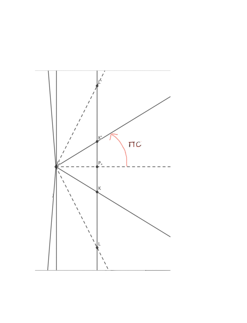
Figure 4. The fundamental sector can be used to tile over the half-plane containing the model line. $P_{*}$ represents the closest point on on the corresponding geodesic to the cone point. Four of the five intersections of the line with the rays forming the boundaries and bisectors of the tiles are marked, L, L’, K, K’. These correspond in pairs to self-intersections of the corresponding geodesic on the cone over the circle of radius c. There are $k+1=3$ tiles and correspondingly $k=2$ self-intersections.

6.1. Integer powers and Metric Quotients

The scattering angle formula (23) shows us that the incoming and outgoing asymptotes of non-collision geodesics are the same precisely when $\frac{1}{c}=n$ for some positive even integer $n$. Recall that $\frac{1}{c}=\beta$ where $\beta$ is the exponent of the Maclaurin transformation $Q\to Q^{\beta}$. If $\beta=n$ is a positive integer (even or odd) then, and only then, does the Maclaurin transformation $Q\mapsto Q^{n}$ become a single-valued map from the folding plane to the Newtonian plane. Under this map, two points $Q,Q^{\prime}$ get mapped to the same point $q$ under this map if and only if they differ by scalar multiplication by some n-th root of unity, which is to say that points on the fibers of the MacLaurin transform are related to each other by integer multiples of rotation by $2\pi/n$. It follows that the map $Q\mapsto Q^{n}$ defines an isomorphism between the quotient space $\mathbb{C}/\mathbb{Z}_{n}$ and the Newtonian plane $\mathbb{C}$. If we take this quotient $\mathbb{C}/\mathbb{Z}_{n}$ to be the metric quotient then we have an algebraic description of our cones with opening angle $2\pi c,c=1/n$, $n=1,2,3,\ldots$.

Some words are in order regarding the adjective “metric” in the phrase ‘metric quotient space’ used just above and used earlier to describe the Kepler cone as $\mathbb{C}/\pm 1=\mathbb{C}/\mathbb{Z}_{2}$. If a finite group $G$ acts isometrically on a metric space $M$, then the quotient space $M/G$ naturally inherits a metric by declaring the distance between two points in the quotient to be the distance between the corresponding orbits in $M$. To obtain the Kepler cone as a metric quotient we take $G=\mathbb{Z}_{2}=\{1,-1\}$ acting on $M=\mathbb{C}=\mathbb{R}^{2}$ by scalar multiplication, putting the standard Euclidean metric on $M$. To obtain these other cones $\mathbb{C}/\mathbb{Z}_{n}$ we use the action by rotation by angles $2\pi j/n$, $j=0,1,2,\ldots$ as realized by scalar multiplication by the group of nth roots of unity.

On any metric space $(M,d)$ we have the notion of a curve being a “geodesic”. To define geodesics on $M$ first assign a length (possibly infinite!) to any continuous curve $c:[a,b]\to M$ in a metric space by using a process of successive ‘polygonal’ approximations. Then declare that a continuous curve is a minimizing geodesic between two points if its length is equal to the distance (i.e $d(c(a),c(b))$) between its endpoints. And declare a curve to be a (not-necessarily minimizing) geodesic if all of its sufficiently short subarcs are minimizing geodesics (between the endpoints of these subarcs). See Burago et al [7] for details.

The metric quotient operation $M\to M/G$ maps geodesics to geodesics. The geodesics on $\mathbb{R}^{2}$ are the straight lines. So the geodesics on these ‘integer cones” $\mathbb{C}/\mathbb{Z}_{n}$ are the quotient images of the straight lines in the $(u,v)$ plane. The metric quotient $\mathbb{C}/\mathbb{Z}_{n}$ is isometric to a cone of angle $2\pi/n$ since a fundamental domain for the action of $\mathbb{Z}_{n}$ is the sector $0\leq\psi\leq 2\pi/n$.

7. Scattering and starbursts: Implications for Non-zero energies

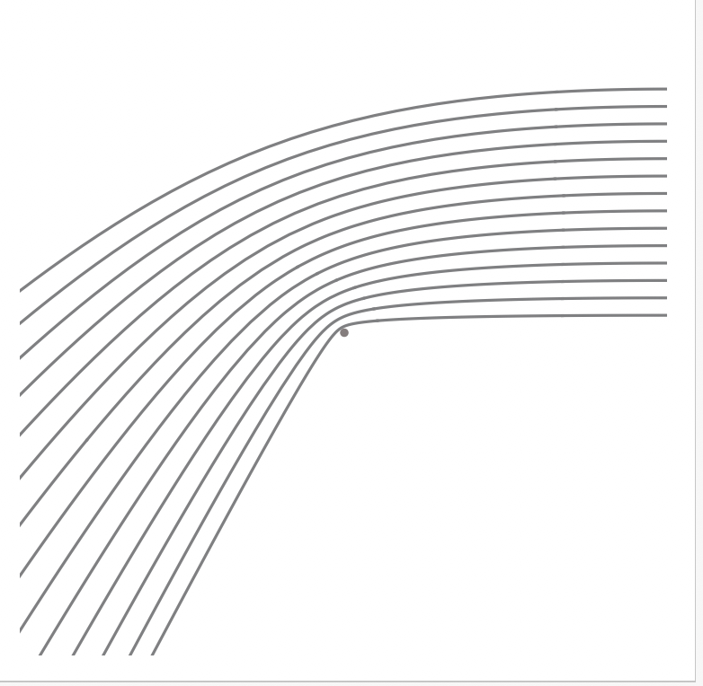
Figure 5. Positive energies. Scattering a half beam with power law $r^{-1/2}$ so $\pi/c=\frac{4\pi}{3}$.

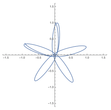
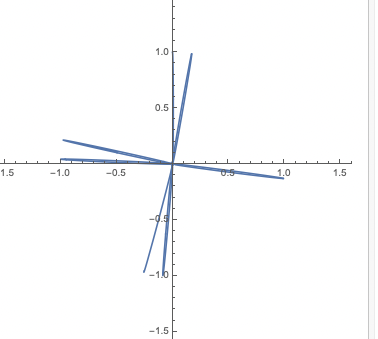
Figure 6. Negative energy solutions, or ‘rosettes’ for $\alpha=2/3$ in which case $\pi/c=\frac{3\pi}{2}$. The rosettes converge to a $\pi/c$ starburst as the angular momentum tends to zero.

Zero-energy solutions with their scattering angle (23) continue to have relevance at non-zero energies. Figures 5 and 6 summarize how. They indicate families of such solutions converging to a curve suffering a collision. In both cases the limiting curve exhibits a change of direction at collision, this change equaling the scattering angle (23). These two figures illustrate

Theorem 4.

Let $\gamma_{\epsilon}(t)$ be a family of non-collision solutions to the $\alpha$-power law problem (equation (10))having energy $E$ and suppose that $\gamma_{\epsilon}$ converges as $\epsilon\to 0$ to a curve $\gamma_{*}$ having a collision. If $0<\alpha<2$ then $\gamma_{*}$ parameterizes a piecewise linear curve whose only vertices (points with changing directions of travel) are at the collision (origin) and the Hill boundary (if there is one). Away from the origin the limiting curve satisfies Newton’s equations. Upon each collision the direction of $\gamma_{*}$ changes, turning by an angle equal to the scattering angle $\pi/c$ with $c=1-\frac{\alpha}{2}$ as usual.

When $E\geq 0$ the limiting curve sweeps out the union of two rays which make an angle equal to the scattering angle. When $E<0$ the solutions are bounded, lying in the Hill disc $r\leq(\mu/E)^{1/\alpha}$ and then the limiting curve is a ‘starburst’ concatenation of brake orbits, with successive orbits making an angle equal to the scattering angle with each other. Figure 5 depicts the positive energy case by exhibiting an incoming half-beam of particles under the influence of an $\alpha=1/2$ power law potential. In the limit as the solutions in the beam tend to the origin their scattering angle limits to $\pi/c=\frac{4}{3}\pi$ as described in the theorem. Figure 6 depicts the negative energy case by showing two negative energy solutions to an $\alpha=2/3$ power law problem. The second solution comes very close to the origin and successive near-brake solutions almost make the angle $\pi/c=\frac{3}{2}\pi$ with each other. The ‘starburst’ aspect of the theorem seems to be a previously unobserved fact regarding power law central force laws.

Setting up a proof. Power law problems, like all central force problems, admit rotational symmetry and conservation of angular momentum

(24) $$J = q\wedge v$$

(25) $$= r^{2}\dot{\theta}.$$

Rotational symmetry means that if $q(t)$ is a solution then so is any rotate $e^{i\theta_{0}}q(t)$ of this solution. The first expression for the angular momentum $J$ in equations (25) uses the two-dimensional version of the cross product $(q,v)\mapsto q\wedge v=(x,y)\wedge(v_{x},v_{y})=xv_{y}-yv_{x}$. The second expression for $J$ in equations (25)uses polar coordinates $(r,\theta)$. Conservation of angular momentum means that $J$ remains constant along solutions. Solutions to central force problems travel along rays through the origin if and only if $J=0$ as one can see from the second expresson for $J$.

If a particular solution to a power law problem with $\alpha\in(0,2)$ tends to the the origin with time then the solution must have $J=0$. We can show this by re-expressing Newton’s equations polar coordinates. The kinetic energy is given by $K=\frac{1}{2}(\dot{r}^{2}+r^{2}\dot{\theta}^{2})$ from which it follows that

$$E=\frac{1}{2}\dot{r}^{2}+\frac{J^{2}}{2r^{2}}-\frac{\mu}{r^{\alpha}}$$

since $r^{2}\dot{\theta}^{2}=\frac{J^{2}}{r^{2}}$. The sum of the last two terms in this rendiction of energy is called the “effective potential” $V_{eff}$:

$$V_{eff}(r;J)=\frac{J^{2}}{2r^{2}}-\frac{\mu}{r^{\alpha}}$$

(Newton’s equations, rewritten in polar coordinates, are $\ddot{r}=-\frac{d}{dr}V_{eff}(r;J)$ together with $\dot{\theta}=\frac{J}{r^{2}}$ and $\dot{J}=0$.) Since $\frac{1}{2}\dot{r}^{2}\geq 0$ we have that $V_{eff}(r;J)\leq E$. It follows that for fixed $E,J$ with $J\neq 0$ the radial variable $r$ lies in the ‘Hill interval” $\{r:V_{eff}(r;J)\leq E\}$. The salient fact for us is that when $J\neq 0$ and $\alpha$ is in our range the left endpoint of the Hill interval is a positive number $r_{min}(E,J)>0$ and that

(26) $$r_{min}(E,J)\to 0\iff J\to 0$$

for $E$ fixed or lying in a bounded interval. (If $E\geq 0$ then the Hill set is of the form $[r_{min}(E,J),\infty)$ while if $E<0$ it has the form $[r_{min}(E,J),r_{max}(E,J)]$ where $r_{max}(E,J)$ is finite.) We can see this fact regarding the Hill interval by graphing $V_{eff}(r;J)$ as a function of $r$ for the parameter $J\neq 0$. See figure 7. We have, for $\alpha$ in our range $(0,2)$, that $\lim_{r\to 0}V_{eff}(r;J)=+\infty,\lim_{r\to\infty}V_{eff}(r;J)=0$ and that $V_{eff}(r;J)$ has only one critical point $r=r_{*}(J)$ in the range $0<r<\infty$ and this critical point is a global minimum whose value is negative. The structure of the Hill interval follows.

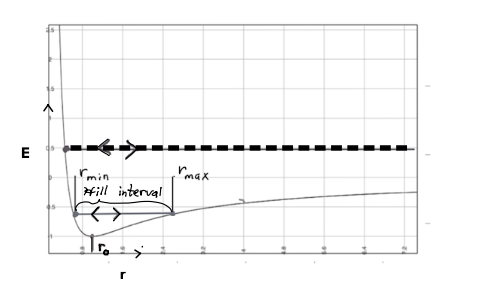
Figure 7. The graph of the effective potential $V_{J}(r)=J^{2}/r^{2}-\mu/r$ for the Kepler problem. I took $J=1,\mu=2$. The horizontal lines represent fixed energy levels. The thin solid one is negative and $r_{0}$ is the circular orbit for this angular momentum. The dotted thicker line represents a positive energy value with corresponding unbounded, or scattering orbit.

Exercise 3.

For $\alpha=2$ show that there are solutions with $J\neq 0$ which are logarithmic spirals, limiting to the origin. Show that whenever $\alpha\geq 2$ there are solutions to the power law problem having $J\neq 0$ but which limit to the origin, spiralling in as they go.

A circular solution space. Fixing $E$ and $J$ defines a family ${\mathcal{F}}(E,J)$ of solutions mapped to itself by rotations. For power law potentials in the range $0<\alpha<2$ the family ${\mathcal{F}}(E,J)$ consists of a single solution modulo rotations and time translations, provided $J\neq 0$ and provided the family is not empty. Theorem 4 concerns $\lim_{J\to 0}{\mathcal{F}}(E,J)$.

Proof of the theorem.

Write $r_{min}(\epsilon)=min_{t}|\gamma_{\epsilon}(t)|$ for the distance from the origin of the solution $\gamma_{\epsilon}$. By hypothesis $r_{min}(\epsilon)\to 0$ with $\epsilon$ so that according to equation (26) we have that its angular momentum $J\to 0$ with $\epsilon$. It follows that away from collisions our limiting curve $\gamma_{*}$ obeys Newton’s equations and has $J=0$ and so lies along rays. That ray may change only upon collision. Proving the theorem amounts to showing that the ray does change at each collision and that the change in angle is precisely the scattering angle.

To verify the change in angle we use an additional space-time scaling symmetry

(27) $$\delta_{\lambda}:q(t)\mapsto\lambda q(\lambda^{-\nu}t);\nu=\frac{\alpha}{2}+1.$$

enjoyed by $\alpha$- power law problems. This transformation takes solutions to solutions, a fact which follows from the homogeneity of the potential $V=-\mu/r^{\alpha}$. This scaling transforms velocities by $v\mapsto\lambda^{-\alpha/2}v$ and energy and angular momentum by $E\mapsto\lambda^{-\alpha}E,J\mapsto\lambda^{1-\alpha/2}J=\lambda^{c}J$. Thus the scaling defines a scaling isomorphism $\delta_{\lambda}:{\mathcal{F}}(E,J)\to{\mathcal{F}}(\lambda^{-\alpha}E,\lambda^{c}J)$ between solution spaces. Here we have used the notation ${\mathcal{F}}(E,J)$ introduced in the remark immediately above for the space (a circle) of all solutions having energy $E$ and angular momentum $J$. Scale invariant properties of these curves, such as the angle between successive perihelion and apihelion when $E<0$, are necessarily preserved by the scaling. Now, set $J=\epsilon$, imagining $\epsilon\to 0$ and set $\epsilon=\lambda^{-c}$ so that $\lambda=1/\epsilon^{1/c}\to\infty$ as $\epsilon\to 0$. The scaling transformation takes ${\mathcal{F}}(E,\epsilon)$ to ${\mathcal{F}}(\lambda^{-\alpha}E,1)={\mathcal{F}}(\epsilon^{\alpha/c}E,1)$. It follows that the scattering angle associated to fixing $E$ and letting $J\to 0$ is the same as the scattering angle associated to fixing $J=1\neq 0$ and letting $E\to 0$. But this is the scattering angle for ${\mathcal{F}}(0,1)$ as described in lemma 3.

QED

7.1. Scattering off power law potentials

Figure 8 is a redrawing of figure 5, to place it into the the context of classical scattering. The figure indicates facts I learned from [13] and which I have summarized below as proposition 2. Understanding and rederiving these scattering fact provided the inspiration for writing this paper. For further reading on classical scattering see the chapter on scattering in [12] and the primary source [21].

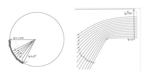
Figure 8. The right panel shows a half beam being scattered by an attractive central force power law $f(r)=r^{-1/2}$. The left panel shows the arc of the circle resulting from the scattering map applied to this half beam, its image being half of the scattered image of the full beam.

Figure 8 depicts a half-beam scattered by an $\alpha=1/2$ power law central force. The parameter $b$ of the figure is a transverse parameter to the rays comprising the beam and $b$ labels the trajectories making up the half-beam. This parameter $b$ coordinatizes a line placed very far from the origin nearly orthogonal to the incoming beam. As $b\to\infty$ the corresponding trajectories recede to infinity, barely affected by the central force. As $b\to 0$ the trajectories tend to collision and so we are in the situation of lemma 3. The limiting trajectory is deflected from that of a straight line by an angle $|\pi/c-\pi|=\pi/3$ as $b\to 0$. The $\pi/c=4\pi/3$ arises from the scattering angle of lemma 3 and we have to subtract $\pi$ because, in our definition of ‘scattering angle’ an undeflected straight line would have ‘scattering angle of $\pi$’ and we are now measuring so that ‘undeflected’ means angle $0$.

The labeling parameter $b$ is known as the impact parameter. Its magnitude is the distance of a line from the origin if the force had been turned off so that no deflection occured. For any $\alpha$-power law with $0<\alpha<2$ the scattering of a positive energy half-beam shares the properties just described in the paragraph above for $\alpha=1/2$. Write $f(b)$ for the angle of deflection of the trajectory labelled by $b$. We have $f(b)\to 0$ as $b\to\infty$ and $f(b)=\frac{\pi}{c}-\pi$ as $b\to 0^{+}$. In between $f(b)$ is continuous. With a bit more work one can show $f$ is monotone $b$ varies over $(0,\infty)$. It follows that

(28) $$f((0,\infty))=(0,A)\text{ where }A=\frac{\pi}{c}-\pi$$

This arc $(0,A)\subset\mathbb{S}^{1}$ describes the arc of outgoing rays which arise from the scattered half-beam.

Now consider scattering a whole beam, so that $b$ ranges over the real line $\mathbb{R}$. The deflection angle $f(b)$ is continuous in $b$ except at $b=0$. By reflectional symmetry of central force dynamics we have that $f(-b)=-f(b)$. Trajectories passing above the center, so with $b>0$ in our figure, swerve to the left while trajectories passing below the center, so with $b<0$, swerve to the right but the magnitude of these two deflections is same for $b$ and $-b$. It follows that $f(\mathbb{R}\setminus\{0\})=(-A,0)\cup(0,A)\subset\mathbb{S}^{1}$ where $A$ is as in equation (28) just above. We have proved:

Proposition 2.

The image of a beam upon scattering by an $\alpha$-power law, $0<\alpha<2$, is an arc of measure $2A=2\pi\frac{\alpha}{2-\alpha}$ with its midpoint deleted. The midpoint corresponds to the direction of the incoming beam and to $lim_{b\to\pm\infty}f(b)$. The endpoints of the arc correspond to the deflection suffered by the two collision limits $lim_{b\to 0^{+}}f(b)$ and $lim_{b\to 0^{+}}f(b)$.

If $\alpha<1$ then $2A<2\pi$ which means the set of scattered rays does not cover the circle. The set of missing rays is an arc centered at “complete backscatter” meaning the direction $\pi$ which is opposite to the incoming beam. The arclength of the missing rays is $2\pi-2A$. On the other hand, if $1<\alpha<2$ then $2A>2\pi$ which means that some outgoing directions are covered more than once: there are two or more incoming rays which scatter out along a particular outgoing direction.

Exercise 4.

Show that impact parameter $b$, angular momentum $J$ and energy $E$ are related by $b=J/\sqrt{2E}$ when we are in the scattering regime, $E>0$.

7.2. Rutherford’s scattering

The Coulomb problem is the Kepler problem but with the sign of the coupling constant reversed so as to make the force repulsive:

(29) $$\ddot{q}=+\mu q/r^{3},$$

with $\mu>0$. It is basic to electromagnetism where $\mu$ becomes proportional to the product of the charges involved, the one at the center and the incoming one. We have $\mu>0$ for like charges and $\mu<0$ for opposite charges. Like charges repel and opposite charges attract. Scattering in the Coulomb problem is almost identical to scattering in the Kepler problem. The sign of the deflection of rays is reversed between the two.

The discovery of the nucleus relied upon Rutherford’s analysis [21] of Coulomb scattering. See figure 9.

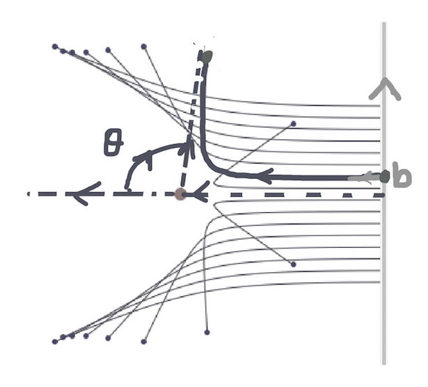
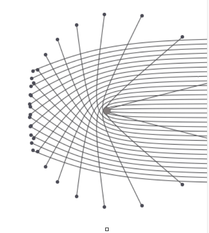
Figure 9. Rutherford Scattering. The variable $b$ is the impact parameter and $\theta$ coordinatizes the direction of outgoing rays.

His lab assistants Geiger (of the counter) and Marsden had been doing experiments in which they directed a high-speed beam of alpha particles (Helium nuclei) at gold foil. They measured the directions of the outgoing particles scattered by the foil and were surprised that a measurable fraction (1/20,000) suffered over a ninety degree change in direction. A few particles suffered a nearly complete recoil. According to the dominant ‘plum pudding model’ of the time, none should be coming back. To explain their experimental results Rutherford replaced the plum pudding mush making up the gold atom’s center with a concentrated point-positive charge containing nearly all the nearly all the mass of a gold atom is concentrated in a point-like positive charge at the center -the nucleus. A much lighter and diffuse cloud of negative charges (electrons) were to surround the nucleus. Alpha particles were known to have positive charge, like the nucleus. The idea was that the alpha particles penetrated the electron cloud with ease at which point they had to contend with the strong repulsive Coulomb force of the nucleus.

Rutherford computed

(30) $$\theta=f(b)=2arctan(\frac{\mu}{2Eb})$$

for Coulomb-Kepler scattering, that is, for equation (29) regardless of the sign of $\mu$. (Note: we just switched sign conventions compared to our original use of the coupling constant in Kepler.) See [21], or [12], particularly p 286, eq (12.3.3), or [14] for this computation.

It is a beautiful fact that the Coulomb-Kepler scattering map $f(b)$ of formula (30) is a stereographic projection $\mathbb{R}\to\mathbb{S}^{1}$. See figure 10.

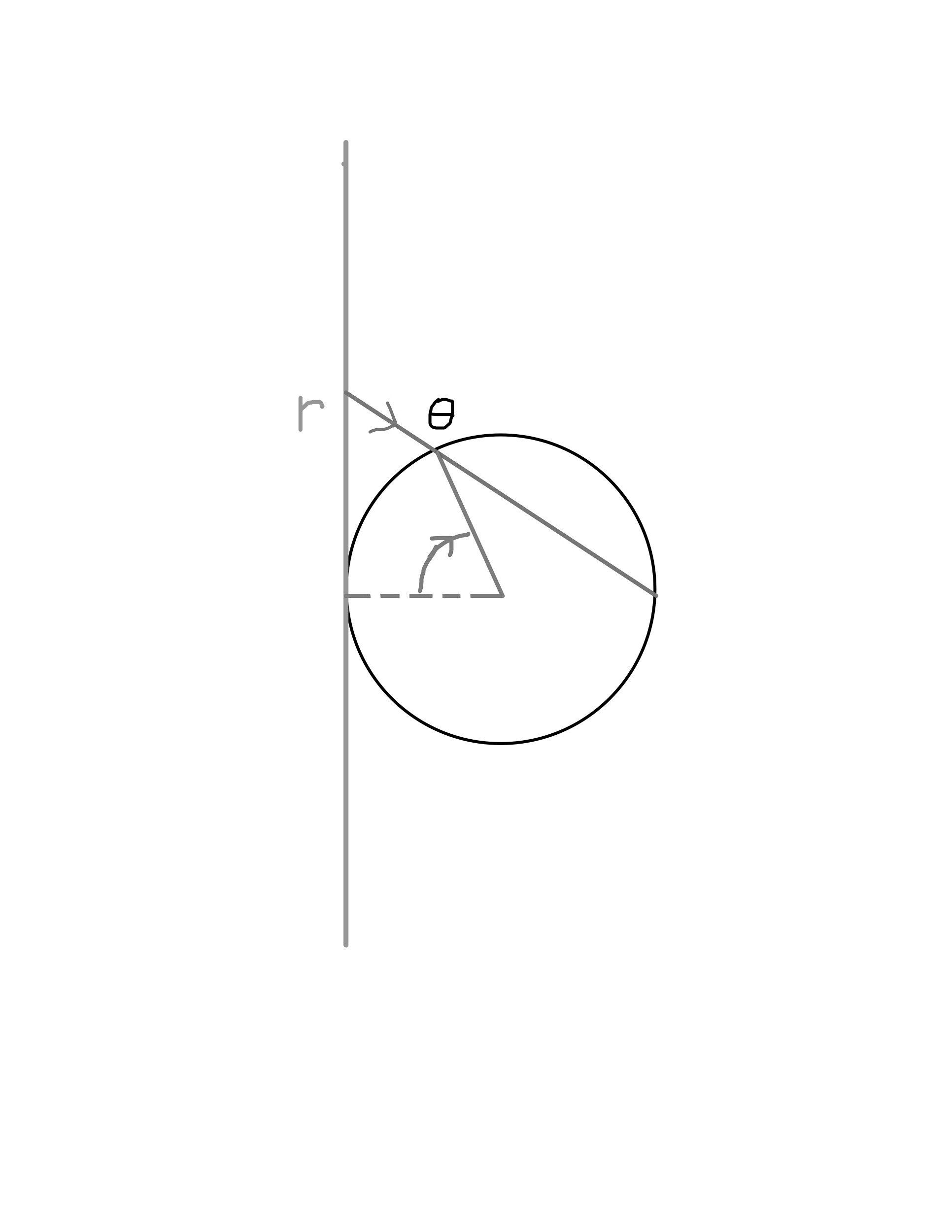
Figure 10. Stereographic Projection. Take $r=b$ on the line.

The expression for the stereographic projection $r\to\theta$ indicated in the figure is $\theta=2arctan(1/r)$. Upon setting $r=2Eb/\mu$ we find that Coulomb scattering and stereographic projection are the same map.

This relation to stereographic projection makes it clear that the Rutherford scattering map covers the circle of outgoing directions exactly once. We have $f(\mathbb{R}\setminus\{0\})=\mathbb{S}^{1}\setminus\{0,\pi\}$. We can complete the map by taking limits: $f(\infty)=0$ and $f(0)=\pi=-\pi$ The fact that the map extends by continuity for the whole compactified real line is essentially equivalent to the single-valuedness of Levi-Civita regularization. An analogous extension holds whenever $\beta=n$ in the Maclaurin transformation, as per subsection 6.1. If we complete the real line to a circle by identifying $+\infty$ to $-\infty$ then the scattering map becomes a degree $n$ analytic map from the circle to itself. For details see [13].

8. Deriving the Jacobi-Maupertuis principle.

We will give two derivations of the JM principle, one Lagrangian, the other Hamiltonian. The first has the advantage of a direct variational viewpoint but the disadvantage of not easily yielding the relation between time and JM arclength.

8.1. Lagrangian Mechanics.

The Lagrangian formulation of classical mechanics is based on choosing a function $L:\mathbb{R}^{n}\times\mathbb{R}^{n}\to\mathbb{R}$ , written $L(q^{i},v^{i})$ so that $(q^{1},\ldots,q^{n},v^{1},\ldots,v^{n})$ are used as coordinates of $\mathbb{R}^{n}\times\mathbb{R}^{n}$. The Euler-Lagrange [EL] equations for $L$ are the ODEs

$$\frac{d}{dt}({{\partial L}\over{\partial v^{i}}})={{\partial L}\over{\partial q^{i}}}$$

supplemented by

$$\dot{q}^{i}=v^{i}.$$

To recover Newton’s equations as EL equations take

$$L(q,v)=\text{ kinetic}-\text{potential}=K(v)-V(q)$$

Exercise 5.

Show that our Newton’s equations (4) are the Euler-Lagrange equations for $L(q,v)=\frac{1}{2}\|v\|^{2}-V(q)$ where $q=(x,y),v=(v_{x},v_{y})$ and $(q^{1},q^{2},v^{1},v^{2})=(x,y,v_{x},v_{y})$.

The Lagrangian connects the calculus of variations to mechanics. Define the action of an absolutely continuous path to $q:[0,T]\to\mathbb{R}^{n}$ to be $\int_{0}^{T}L(q(t),\dot{q}(t))dt$. Consider the “standard problem of the calculus of variations”: to minimize the action among all paths joining two fixed endpoints $q_{0},q_{1}$ in a time $T$. The minimizer, if it exists, and if it is twice-differentiable, must satisfy the EL equations and hence Newton’s equations.

Example 1 (Riemannian geometry).

A Riemannian metric is given in local coordinates by a Lagrangian which is quadratic positive-definite in velocities:

(31) $$L(q,v)=\frac{1}{2}\Sigma g_{ij}(q)v^{i}v^{j}$$

where the $q$-dependent matrix $g_{ij}(q)$ is symmetric positive-definite. $2L$ represents the square of the infinitesimal element of arclength $ds$. One writes $ds^{2}=\Sigma g_{ij}(q)dq^{i}dq^{j}$. The length of a path is defined to be $\int ds=\int\sqrt{\Sigma g_{ij}(q(t)\dot{q}^{i}\dot{q}^{j}}dt$ and is independent of how the curve $q(t)$ is parameterized. The geodesic equations are the EL equations for $L$. A judicious application of the Cauchy Schwartz inequality shows that a curve is a minimizer for the standard problem of the calculus of variations for $L$ if and only if it both minimizes the total length among all paths joining the specified endpoints and is parameterized so as to have constant speed: $L(q(t),\dot{q}(t))=const.$.

8.1.1. Heuristic Lagrangian proof of JM formulation of mechanics

Write $U=-V$ for the negative of the potential. Then Newton’s equations are the Euler-Lagrange equations for the Lagrangian $L(q,v)=K(v)+U(q)$. At energy $E=0$ we have $U\geq 0$ on the Hill region. Using $a^{2}+b^{2}\geq 2ab$ with equality iff $a=b$ we get that $K+U\geq 2\sqrt{KU}$ with equality if and only if $K=U$, which is to say, iff $E=0$. Now integrate with respect to $t$ along any path. We get $\int Ldt\geq\int 2\sqrt{KU}dt$. But $2\sqrt{KU}dt=\sqrt{2U}|\dot{q}|dt=ds_{JM}$ is the zero energy JM arclength for curves parameterized by Newtonian time $t$. So

$$\int_{q[0,T]}Ldt\geq\int_{q([0,T])}ds_{JM}$$

with equality between the integrals if and only if $E(q(t),\dot{q}(t))=0$ along the path of integration $q$. Now recall the connection to the calculus of variations. The EL equations are the extremal equations associated to the action, the integral of $L$ over paths. In the formulation above of the standard problem in the calculus of variations we fixed both the endpoints $q_{0},q_{1}$ of paths, and also the time of travel $T$ between these endpoints. Relax the time travel condition so as to allow any time of flight between the two points. We have shown that minimizers for this relaxed problem must have zero energy. They will also satisfy the EL equations by the standard argument of the calculus of variation, and, being JM arclength minimizers, must be JM geodesics. We have shown that the free-time action minimizers must (a) have zero energy and (b) be a zero-energy JM geodesic.

“QED”

The astute reader will see various problems implicit in the above “proof”. We will not try to fix them, but leave them as challenges to the reader. Instead, we will describe the simple trick which allows us to promote this heuristic argument to any energy $E$.

If we replace the potential $V$ by $V+c$, $c$ a constant, we get the same Newton’s equations. It follows that if we replace $U$ by $U+E$ for $E$ a constant in the Lagrangian we still get Newton’s equations as the EL equations. Now $K=a^{2}$ but $b=\sqrt{U+E}$ where we need $U+E\geq 0$ so that we are working on the Hill’s region. We get that the modified action $\int(K+U+E)dt$ is greater than or equal to the energy $E$ JM arclength $\int 2\sqrt{K}\sqrt{U+E}dt$, and that the free-time minimizers of the modified action must be both solutions to Newton’s equation having energy $E$, when parameterized by time, and a JM-geodesic with respect to the energy $E$ JM metric.

8.2. Hamiltonian formalism.

In the Lagrangian formulation we work with positions and velocities. In the Hamiltonian version we work with positions and momenta. To explain the difference it will help to replace $\mathbb{R}^{n}$ by an abstract real finite-dimensional vector space $\mathbb{V}$. This $\mathbb{V}$ is meant to encode the position of our “mechanical system”. If $q(t)$ is a curve in $\mathbb{V}$ its derivative $v(t)=\dot{q}(t)$ is also a curve in $\mathbb{V}$. So velocities are vectors $v\in\mathbb{V}$. Momenta on the other hand are dual vectors $p\in\mathbb{V}^{*}$. The Lagrangian is a function on $L:\mathbb{V}\times\mathbb{V}\to\mathbb{R}$ while the Hamiltonian is a function $H:\mathbb{V}\times\mathbb{V}^{*}\to\mathbb{R}$.

The Legendre transformation

$$FL:\mathbb{V}\times\mathbb{V}\to\mathbb{V}\times\mathbb{V}^{*};FL(q,v)=(q,{{\partial L}\over{\partial v}}(q,v))$$

mediates between the Lagrangian and Hamiltonian formalisms. Some words are in order regarding the partial derivative ${{\partial L}\over{\partial v}}$ and why it takes values in $\mathbb{V}^{*}$. Freeze $q$ and consider the function $f(v)=L(q,v)$, $f:\mathbb{V}\to\mathbb{R}$. Then $df(v_{0})(h)=\frac{d}{d\epsilon}f(v_{0}+\epsilon h)$, valid for all $h\in\mathbb{V}$ and so $df(v_{0})={{\partial L}\over{\partial v}}(q,v_{0})\in\mathbb{V}^{*}$ What is important is that $p={{\partial L}\over{\partial v}}(q,v)\in\mathbb{V}^{*}$.

Exercise 6.

A. Suppose that $\mathbb{V}=\mathbb{R}$ is one-dimensional. and $L(q,v)=\frac{1}{2}mv^{2}-V(q)$. Compute that $FL(q,v)=(q,mv)$ so that momentum is given by the usual formula $p=mv$.

B. Suppose that $\mathbb{V}=\mathbb{R}^{n}$ and $L(q,v)=\frac{1}{2}\Sigma m_{a}(v^{a})^{2}-V(q)$. Then the momentum components of $p={{\partial L}\over{\partial v}}(q,v)$ are given by $p_{a}=m_{a}v^{a}$. Here we have invoked the identification $\mathbb{R}^{n}=(\mathbb{R}^{n})^{*}$ induced by the canonical basis, or, what is the same, by the standard inner product. In this way $p=(m_{1}v^{1},\ldots,m_{n}v^{n})\in\mathbb{R}^{n}$.

C. Suppose that $\mathbb{V}$ is endowed with a Euclidean inner product $\langle,\cdot,\cdot\rangle$ and that $L(q,v)=\frac{1}{2}\langle v,v\rangle-V(q)$. Show that $p={{\partial L}\over{\partial v}}(q,v)$ is given by metric duality: $p:\mathbb{V}\to\mathbb{R}$ is the linear functional $p(w)=\langle v,w\rangle$.

D. Return to the example of Riemannian geometry above. Show that ${{\partial L}\over{\partial v}}(q,v)_{i}=\Sigma g_{ij}(q)v^{j}$. In other words, if I write $\langle v,w\rangle_{q}=\Sigma g_{ij}(q)v^{i}w^{j}$ then $FL(q,v)=(q,p)$ with $p(w)=\langle v,w\rangle_{q}$.

Exercise 7.

Show that the EL equations are the ODEs $\frac{d}{dt}FL(q,v)=(v,{{\partial L}\over{\partial q}}(q,v))$ on $\mathbb{V}\times\mathbb{V}^{*}$.

The differential $dV(q)$ of $V$ at a point $q\in\mathbb{A}$ is an element of the dual space $\mathbb{V}^{*}$ defined by $dV(q)(h)=\frac{d}{d\epsilon}V(q+\epsilon h)$. The gradient of $V$ is defined by

$$dV(q)(h)=\langle\nabla V(q),h\rangle.$$

To get the Hamiltonian formalism we use the Legendre transformation to change variables from $(q,v)$ to $(q,p)$. This is most simply done when the transformation is invertible. Suppose this is so. Define the Hamiltonian $H:\mathbb{V}\times\mathbb{V}^{*}\to\mathbb{R}$ by $H(q,p)=p(v)-L(q,v)$ where $(q,v)=FL^{-1}(q,p)$.

Assume now that the Legendre transformation is invertible. Then, as the reader can verify without much difficulty, the EL equations can be rewritten in the equivalent form

$$\dot{q}={{\partial H}\over{\partial p}}(q,p),\dot{p}=-{{\partial H}\over{\partial q}}(q,p).$$

known as Hamilton’s equations. Note the consistency: ${{\partial H}\over{\partial q}}(q,p)\in\mathbb{V}^{*}$ since the partial derivative (differential) is with respect to $q\in\mathbb{V}$, while ${{\partial H}\over{\partial p}}\in\mathbb{V}^{**}=\mathbb{V}$ since the differential is with respect to $p\in\mathbb{V}^{*}$.

Exercise 8.

Return to example C above where the Lagrangian is $L(q,v)=K(v)-V(q)$ with $K(v)=\frac{1}{2}m\langle v,v\rangle$, with $q,v\in\mathbb{V}$ a real vector space $\mathbb{V}$ endowed with a Euclidean structure $\langle\cdot,\cdot\rangle$. The corresponding EL equations are equivalent to the first order form of Newton’s equations

$$\ddot{q}=-\nabla V(q)$$

Note the Euclidean structure enters in obtaining the gradient of $V$ via $dV(q)(w)=\langle\nabla V(q),w\rangle$. The Hamiltonian is $H(q,p)=K^{*}(p)+V(q)$ where $K^{*}$ is the quadratic form associated to the dual metric induced by the inner product on $\mathbb{V}$ which led to the kinetic energy $K$. The reader can verify directly that Hamilton’s equations, Newton’s equations and the EL equations are rewrites of each other, the Legendre transformation $p=\langle v,\cdot\rangle$ being the change of variables from velocity to momentum.

Show that if $L(q,v)=\frac{1}{2}\Sigma g_{ij}(q)v^{i}v^{j}$ is the Lagrangian for a Riemannian geometry then $H(q,p)=\frac{1}{2}\Sigma g^{ij}(q)p_{i}p_{j}$ is the corresponding Hamiltonian. Thus the geodesics are the configuration projections $q(t)$ of solutions $(q(t),p(t))$ to this $H$’s Hamilton’s equations. Show that a geodesic is parameterized by arclength if and only if $H(q(t),p(t))=1/2$.

Consider the special case where $L(q,v)=\frac{1}{2}\lambda(q)|v|^{2}$ where $|v|^{2}=\Sigma(v^{i})^{2}$. Show that $H(q,p)=\frac{1}{2}\frac{1}{\lambda(q)}|p|^{2}$.

A wee bit of symplectic geometry. The domain $\mathbb{E}=\mathbb{V}\times\mathbb{V}^{*}$ of Hamilton’s equations is known as phase space. and write vectors of $\mathbb{E}$ in the form $(V_{q},V_{p})$ so that $V_{q}\in\mathbb{V},V_{p}\in\mathbb{V}^{*}$.

Definition 4.

The canonical two-form on $\mathbb{E}$ is the bilinear skew-symmetric form $\omega:\mathbb{E}\times\mathbb{E}\to\mathbb{R}$ given by $\omega((V_{q},V_{p}),(W_{q},W_{p}))=(W_{p}(V_{q})-V_{p}(W_{q})$. $\omega((q,p),(q^{\prime},p^{\prime}))=p^{\prime}(q)-p(q^{\prime})$.

The form $\omega$ is non-degenerate, which means that the linear map

$$J:\mathbb{E}\to\mathbb{E}^{*}\text{ defined by }Z\mapsto\omega(Z,\cdot)$$

is a vector space isomorphism.

Definition 5.

A symplectic form is a non-degenerate skew-symmetric form on a vector space. A symplectic vector space is a vector space endowed with a symplectic form.

A symplectic vector space must have even dimensions. Any two symplectic vector spaces (like any two inner product spaces) of the same dimension are isomorphic as symplectic vector spaces.

If $(\mathbb{E},\omega)$ is a symplectic vector space and function $H:\mathbb{E}\to\mathbb{R}$ is a smooth function then we can define its Hamiltonian vector field, or “symplectic gradient” by

$$\omega(sgradH,Z)=dH(z)(Z).$$

valid for all vectors $Z$ in $\mathbb{E}$ and all points $z\in\mathbb{E}$. Here $dH(z)\in\mathbb{E}^{*}$ is the differential of $H$. Equivalently

$$sgrad(H)=JdH$$

Exercise 9.

Verify that $sgradH=({{\partial H}\over{\partial p}},-{{\partial H}\over{\partial q}})$

Verify that $dH(sgradH)=0$.

Definition 6.

A level set $\{F=c\}$ of a smooth function on a vector space is said to be “non-degenerate” if $dF(p)\neq 0$ whenever $F(p)=c$.

The implicit function theorem asserts that a non-degenerate level set $\Sigma=\{p:F(p)=c\}$ is a smooth hypersurface and that the tangent spaces to $\Sigma$ are swept out by the kernels of $dF$. In other words, $T_{p}\Sigma=ker(dF(p))$ whenever $p\in\Sigma$.

Corollary 1.

If two different functions on phase space share the same non-degenerate level set, then their Hamiltonian vector fields are parallel along this level set.

Proof. Write $H$ and $F$ for the two functions and $\Sigma$ for their common level set. Thus $\Sigma=\{H=c_{1}\}=\{F=c_{2}\}$ for constants $c_{1},c_{2}$. The tangent space to $\Sigma$ at any point $z$ is a codimension $1$ hyperplane equal to both the kernel of $dH(z)$ and to the kernel of $dF(z)$. It follows that $dF(z)=\lambda(z)dH(z)$ holds along $\Sigma$ for some smooth nowhere zero scalar function $\lambda:\Sigma\to\mathbb{R}$. Applying $J$ we get that $sgradG(z)=\lambda(z)sgradH(z)$, valid along $\Sigma$. QED

8.3. Hamiltonian proof of the JM reformulation of Mechanics

The geodesics for the JM metric at energy $E$ are generated by the Lagrangian $L_{JM}=\frac{1}{2}(2(E-V(q)))|v|^{2}$. Its corresponding Hamiltonian is $F(q,p)=\frac{1}{2}\frac{1}{2(E-V(q))}|p|^{2}$. To get geodesics parameterized by arclength we must set $F=\frac{1}{2}$. Note: $F=\frac{1}{2}\iff\frac{1}{2(E-V(q)}|p|^{2}=1\iff\frac{1}{2}|p|^{2}=E-V(q)\iff\frac{1}{2}|p|^{2}+V(q)=E$. We have shown that the level set $F=1/2$ equals the level set $H=E$. By the above corollary, this proves that $sgrad(F)(z)=\lambda(z)sgrad(H)(z)$ holds for $z\in\Sigma$, assuming that the level set is non-degenerate. Indeed, a peek into the proof of the corollary shows that we can relax the assumption that the entire level set be non-degenerate so that the corollary holds at all points $z$ for which both $dF(z)$ and $dH(z)$ are nonzero. Since both functions are quadratic in $p$ this non-degeneracy holds wherever $p\neq 0$, which is to say, away from the Hill boundary. (The level set is non-degenerate if and only there are no critical points of the potential for which $V(q)=E$.)

To get the reparameterization formula relating $s$ and $t$ we find $\lambda(q)$. And to find $\lambda(q)$ we write out the q-part of the two Hamilton’s equations. We have, for Newtonian version that $\dot{q}=p$ (our masses are all “$1$”). On the other hand, for the JM geodesic equations we have that $\frac{dq}{ds}=\frac{1}{2(E-V(q)}p$. I claim that it follows that $\lambda(q)=\frac{dt}{ds}=\frac{1}{2(E-V(q)}$. Indeed, we can write Newton’s equations as $(\frac{dq}{dt},\frac{dp}{dt})=(X_{1},X_{2})$ where $sgrad(H)=(X_{1},X_{2})$ and we can write the geodesic equations as $(\frac{dq}{ds},\frac{dp}{ds})=(Y_{1},Y_{2})$ where $sgrad(F)=(Y_{1},Y_{2})$. By the corollary, along $\Sigma$ we have that $Y_{i}=\lambda(q)X_{i}$. But we have just shown that $X_{1}=p$ while $Y_{1}=\frac{1}{2(E-V(q)}p$. Now use $\frac{d}{ds}=\frac{dt}{ds}\frac{d}{dt}$.

QED

9. Acknowledgements

I thank Alain Albouy and Andreas Knauf for conversations and history and Gil Bor with help making the pictures. I thank the support of a Simons Foundation Travel grant, award number 674861, which helped to make this work possible.

References

- [1] Albouy, A. and Zhao, Lei, Darboux Inversions of the Kepler Problem Regular and Chaotic Dynamics, 2022, v. 27, no. 3, pp. 253- 280 , (2022).
- [2] Arnol’d, V. I. and Vasiliev, V. A., Addendum to: Newton’s Principia Read 300 Years Later, Notices Amer. Math. Soc., v. 37, no. 2, p. 144, (1990).
- [3] Arnol’d, V. I., Huygens and Barrow, Newton and Hooke, Basel: Birkhauser, (1990).
- [4] Bertrand, J., Théorème relatif au mouvement d’un point attirè vers un centre fixe, C. R. Acad. Sci. Paris, v. 77, no. 16, pp. 849-853, (1873).
- [5] Bertrand, J., Sur la possibilitè de déduire d’une seule des lois de Kepler le principe de l’attraction, C. R. Acad. Sci. Paris, ,v. 84, pp. 671-674, (1877).
- [6] Bohlin, K., Note sur le problème des deux corps et sur une intégration nouvelle dans le problème des trois corps, Bull. Astron. (1), , v. 28, pp. 113-119, (1911).
- [7] Burago, D., Burago, Y., and Ivanov, S. , A Course in Metric Geometry, Graduate studies in math., 33, AMS pub., Providence, R.I., (2001).
- [8] Darboux,G., Remarque sur la communication précédente,C.R.Acad.Sci.Paris, v.108, pp.449-450, (1889).
- [9] Faure, R., Transformations conformes en mécanique ondulatoire, C. R. Acad. Sci. Paris, v. 237, pp. 603-605, (1953).
- [10] Faure, R., Transformation conforme en mécanique ondulatoire généralisation de la notion de valeur propre, in Proc. of the Internat. Congr. of Mathematicians (Amsterdam, Sept 1954): v.2, pp.337- 339. (1954).
- [11] Goursat, E., Les transformations isogonales en Mécanique, C.R.Acad.Sci.Paris, vol.108,pp.446 -448, (1889).
- [12] Knauf, A., Mathematical Physics: Classical Mechanics, Springer, (2012).
- [13] Knauf, A. and Krapf, M. , The non-trapping degree of scattering, Nonlinearity, 21 2023-2041, (2008).
- [14] Landau, I. and Lifshitz, E. Mechanics, Pergamon Press, (1976).
- [15] Levi-Civita, T., Sur la résolution qualitative du problème restreint des trois corps, in Verhandlungen des dritten Internationalen Mathematiker-Kongresses in Heidelberg, v. 8. bis 13. pp. 402- 408, August 1904, Leipzig: Teubner, (1905).
- [16] Maclaurin, C., Treatise of Fluxions: In 2 Vols., Edinburgh: Ruddimans, 1742.
- [17] McGehee, R., Double Collisions for a Classical Particle System with Nongravitational Interactions, Comment. Math. Helv., v. 56, no. 4, pp. 524?557, (1981).
- [18] Painlevé, P., Mémoire sur la transformation des équations de la Dynamique , J. Math. Pures Appl. (4), v. 10, pp. 5-92, (1894).
- [19] Painlevé, P., Sur les transformations des équations de la Dynamique, C. R. Acad. Sci. Paris, v. 123, pp. 392-395.
- [20] Ricci, M. M. G. and Levi-Civita, T., Méthodes de calcul différentiel absolu et leurs applications, Math. Ann., v. 54, pp. 125-201, (1901).
- [21] Rutherford, E., The Scattering of and Particles by Matter and the Structure of the Atom, Philosophical Magazine. Series 6, v. 21, p. 669-688, (1911). https://www.lawebdefisica.com/arts/structureatom.pdf
- [22] Wintner, A., The Analytical Foundations of Celestial Mechanics, Princeton Math. Series, v. 5, Prince- ton, N.J.: Princeton Univ. Press, (1941).