Pathwise and distributional approximations of semi-Markov processes

Martin Bladt Andreea Minca  and  Oscar Peralta
Abstract.

Continuous-time semi-Markov finite state-space jump processes are considered, inspired by a duration-dependent life insurance model. New approximations using grid-conditional homogeneous Markov jump-processes are developed, based on a recent adaptation of the uniformization principle which results in a strong pathwise convergent sequence of jump processes. Unlike traditional methods that use classical approximations to integro-differential equation solutions to compute their value functions, the proposed grid-conditional homogeneous Markov jump-processes allows for a direct and tractable approximation. In particular, these approximations simplify to easily implementable expressions, making them useful in areas where evaluating pathwise distributional functionals is difficult. Our homogeneous approximation, initially of a grid-conditional kind, is evolved into an unconditional version that holds well under fair regularity assumptions. The practicality of this approach is demonstrated on a disability life insurance model, with realistic underlying semi-Markov process parameters, showcasing its broader applicability in operations research and related fields.

1. Introduction

The traditional mathematical treatment of life insurance is centered around mortality tables and discrete-time computations, with virtually no connection to probability theory or continuous-time models. Around 1875, the Danish astronomer and mathematician Thorvald Thiele introduced the differential equation that governs the net premium reserve of a basic life insurance model, marking the first instance that a continuous-time life insurance framework was formally considered. Many decades later, [Sverdrup, 1952, Hickman, 1964] suggested formal probabilistic approaches for some special cases, while the full continuous-time finite-state Markov jump-process framework was first systematically considered in [Hoem, 1969].

Since the formulation of the basic Markov model, and compounded by the consequential fact that a substantial number of industries in northern European countries have by now adopted continuous-time models, there has been a continuing theoretical and practical demand for extending such models to more flexible stochastic frameworks. Some notable cases have been stochastic mortality rate models (cf. [Cairns et al., 2008]), the integration of financial mathematics and life-insurance concepts (cf. [Steffensen, 2006]), and the introduction of a semi-Markov framework (cf. [Hoem, 1972], see also a modern treatment in [Buchardt et al., 2015]). The literature in these directions nowadays is vast and in constant expansion.

In this paper, we concentrate on the semi-Markov model, a duration-dependent stochastic process, within the context of general life insurance models featuring duration-dependent payments. Semi-Markov processes, first studied in their time-homogeneous version, represent jump processes where interarrival times are not exponentially-distributed, unlike time-homogeneous Markov processes. These are also known as Markov renewal processes in the literature. The seminal works of [Lévy, 1954], [Smith, 1955], and [Cinlar, 1969] laid out the foundational groundwork for these objects. Further, in a life-insurance framework, a time-inhomogeneous version of these processes which considers the jump behavior dependent on both time and the elapsed time since the last jump was explored in [Hoem, 1972, Janssen and De Dominicis, 1984]. For brevity in this paper, we refer to the time-inhomogeneous semi-Markov model simply as ‘semi-Markov’.

The limitations of simple Markovian models in accurately capturing life insurance products are well documented in both practice and literature, as seen in [Janssen, 1966, Hoem, 1972, Buchardt et al., 2015]. While there are some special cases that allow for a clearer mathematical treatment akin to the Markov case, the general scenario remains methodologically complex and numerically delicate. This complexity is due to the requirement for both the transition rates and probabilities of the underlying process in valuation, which for non-trivial multi-state structures often necessitates solving Thiele’s or Kolmogorov’s differential equations. Solutions to these equations are typically approximated using Runge-Kutta-type iterative methods. An efficient Monte Carlo scheme is proposed in [Fox and Glynn, 1986], however, this is applicable only to time-homogeneous semi-Markov processes.

Here, we propose a novel and general-purpose approximation that circumvents the setup of differential equations. Specifically, under notably robust conditions, we systematically construct a tractable process whose paths almost surely converge to those of the semi-Markov model in question, extending the results presented in [Bladt and Peralta, 2022] from time-inhomogeneous to semi-Markov processes. Heuristically speaking, the proposed approximation entails constructing the semi-Markov model by means of uniformization (cf. [Jensen, 1953], see also [Van Dijk, 1992] for the inhomogeneous case) atop a Poisson process of high intensity. The idea can be considered as a pathwise strong convergence version of the Uniform Acceleration method [Massey and Whitt, 1998], and for the more general setting of semi-Markov models. The main novel idea consists in replicating the exact same sequence of states atop another Poisson process that is identically distributed and independent from the original one. Conditional on the arrival times of the original Poisson process, referred from here on as grid-conditional, this approximation is a simple time-homogeneous Markov jump process with transition probabilities that exhibit an algorithmically tractable closed expression. Furthermore, under additional continuity assumptions on the underlying jump intensities, we present an unconditional time-homogeneous Markov jump process with transition probabilities that converge to those of the original semi-Markov model.

As a particular consequence of our convergence results, we obtain a valuation approximation with explicit components that is guaranteed to approximate the target value function to arbitrary precision. Another implicit consequence is the generalization of absorption-time approximations as given in Section 4 of [Ahmad et al., 2023]. Our construction can be regarded as a general result in applied probability which may be employed in any setting where approximating value functions (or other functionals) of a semi-Markov process is of interest. In particular, we believe that continuous-time life insurance mathematics is an application well-suited to demonstrate our results in an elegant and practically useful manner. Several extensions emerge from our study. First, in Section 5.2 we suggest how to apply our framework to reduced form credit risk modeling, where the states can represent ratings of a company and we seek to evaluate a defaultable bond. Secondly, in section 5.3, we show that under mild conditions, the approximation framework also holds for controlled semi-Markov processes, broadening the scope and applicability of our methodology beyond life insurance product valuation. We also suggest how to use our approximation for value functions in optimal control problems.

The remainder of the paper is structured as follows. In Section 2 we introduce the life insurance setup, and the underlying Semi-Markov process. In Section 3 we introduce our general grid conditional approximation. In Section 4, we provide unconditional approximations, under entry-wise Lipschitzness of the intensity matrix. Section 5 provides illustrations and extensions. Technical proofs may be found in Appendices A and B.

2. Preliminaries

This section provides some of the relevant background in the continuous-time life insurance formulation, and on the definition and construction of semi-Markov processes. We return to the former once the main strong approximation is established, while the latter motivates the construction principle of the approximating sequence.

2.1. Life insurance setup

This section introduces the standard setup for a multi-state life insurance model. For readers interested in the simpler Markov case, a comprehensive treatment is presented in [Asmussen and Steffensen, 2020, Chapter V]. We present the semi-Markov model originally introduced in [Hoem, 1972] and also discussed with modern notation in [Buchardt et al., 2015].

Consider an insurance policy issued at time 00 with a terminating time $T\in(0,\infty)$, beyond which there is no more coverage. We deal with a càdlàg stochastic process, defined on a probability space $(\Omega,\mathcal{F},\mathds{P})$, taking values in a finite set $\mathcal{J}=\{1,\dots,J\}$. This set corresponds to different states of the policy. The stochastic process denoting the state of the policy at any given time is given by $Z=\{Z(t)\}_{t\geq 0}$ and is commonly referred to as the multi-state model. We define

(2.1) $$U(t)=\inf\{r>0:Z(t-r)\neq Z(t)\},$$

as the elapsed time since the last jump. We will refer to $U=\{U(t)\}_{0\leq t\leq T}$ as the duration process. In this paper, we are interested in multi-state models $Z$ such that the bivariate process $(Z,U)$ is Markovian, known as semi-Markov processes. We will develop a deeper understanding of semi-Markov models in Subsection 2.2; for now, its definition will suffice.

When considering the value of a policy at any time other than inception, an updated amount will depend on the information available at time $t\in[0,T]$, including the duration process. For that reason, we denote by $\mathcal{F}_{t}$ the $\mathds{P}$-completed natural filtration of $(Z,U)$ up to time $t$. Furthermore, we define the $J$-dimensional counting process $N=(N^{1},\dots,N^{J})$ as

$$N^{k}(t)=\sum_{s\in[0,t]}{\mathds{1}}\{Z(s)=k,Z(s-)\neq k\},\quad k\in\mathcal{J},$$

which counts the number of jumps into state $k$ experienced up to time $t$. Here, $Z(0-)$ is defined as an artificial state $\dagger$ for convenience.

Assume that $B^{k,u}(t)$ denotes, for each $k\in\mathcal{J}$ and $u\geq 0$, a deterministic payment rate process for when $Z(t)$ is in state $k$. We decompose it into its absolutely continuous and discrete parts by

$$B^{k,u}(t)=\int_{0}^{t}b^{k,u}(s)\mathrm{d}s+\sum_{s\in[0,t]}\Delta B^{k,u}(s),$$

where $\Delta B^{k,u}(s)=B^{k,u}(s)-B^{k,u}(s-)$. Similarly, for payments occurring during state transitions, we define $b^{(j,u),(k,v)}(t)$ as the lump-sum payment occurring when transitioning from state $j$ with duration $u$ to state $k$ with duration $v$ at time $t$. Note that the only possible transitions occur for $v=0$.

Combining the above components, the total amount of benefits minus premiums is defined as the stochastic process

$$\begin{split}\mathrm{d}B(t)&=\mathrm{d}B^{Z(t),U(t)}+\sum_{(k,u)\neq(Z(t-),U(t-))}b^{(Z(t-),U(t-)),(k,u)}(t)\mathrm{d}N^{k}(t)\\ &=\mathrm{d}B^{Z(t),U(t)}+\sum_{k\neq Z(t-)}b^{(Z(t-),U(t-)),(k,0)}(t)\mathrm{d}N^{k}(t).\end{split}$$

Introducing the concept of return on investment for the portfolio and denoting an associated nonnegative deterministic interest rate $r(t)$ for $t\geq 0$, we may become interested in the discounted process

$$\int_{t}^{T}e^{-\int_{t}^{s}r}\mathrm{d}B(s),$$

for the valuation of the insurance policy. Here, we use the shorthand notation $\int_{t}^{s}r=\int_{t}^{s}r(u)\mathrm{d}u$. For instance, its first conditional moment given the information at time $t$ is called the reserve:

$$V(t)=\amsmathbb{E}\left[\int_{t}^{T}e^{-\int_{t}^{s}r}\mathrm{d}B(s)\mid\mathcal{F}_{t}\right],$$

while higher-order moments are usually of significant but secondary importance. The function $V$ represents the mean value of all future payments up to time $n$, given the information available at time $t$. Typically, most payment strategies are pre-set, and the condition $V(0-)=0$ (at inception, all total future payments should, on average, cancel out) is used to determine the last free coefficient to produce an actuarially fair contract.

By the semi-Markov property, we have

$$V(t)=\amsmathbb{E}\left[\int_{t}^{T}e^{-\int_{t}^{s}r}\mathrm{d}B(s)\mid Z(t),U(t)\right],$$

and so we now define the function of interest:

$$V(t;i,u)=\amsmathbb{E}\left[\int_{t}^{T}e^{-\int_{t}^{s}r}\mathrm{d}B(s)\mid Z(t)=i,U(t)=u\right],\quad k\in\mathcal{J},\>u\geq 0.$$

2.2. Semi-Markov jump processes

Let $Z=\{Z(t)\}_{t\geq 0}$ be a càdlàg stochastic process, defined on the probability space $(\Omega,\mathcal{F},{\amsmathbb P})$, with state space $\mathcal{J}=\{1,2,\dots,J\}$. We say that $Z$ is a semi-Markov process if for all $0<t<s$ and $i\in\mathcal{J}$,

$\displaystyle{\amsmathbb P}(Z(s)=j\,|\,Z(r),0\leq r\leq t)={\amsmathbb P}(Z(s)=j\,|\,Z(t),U(t)),$

where

(2.2) $$U(t)=\inf\{r>0:Z(t-r)\neq Z(t)\}.$$

The process $U=\{U(t)\}_{t\geq 0}$ is termed the duration process associated with $Z$.

In this work, we will focus on the class of semi-Markov processes that are time-inhomogeneous, in the sense of [Janssen and De Dominicis, 1984], and are driven by a family of intensity matrices $\{\bm{\Lambda}(s,v)\}_{s,v\geq 0}$ (where $\bm{\Lambda}(s,v)=\{\Lambda_{ij}(s,v)\}_{i,j\in\mathcal{J}}$) possessing the following characteristics:

  • For all $v\geq 0$, the mapping $s\mapsto\bm{\Lambda}(s,v)$ is càdlàg,

  • For all $s\geq 0$, the mapping $v\mapsto\bm{\Lambda}(s,v)$ is càdlàg,

  • There exists $\gamma_{0}\leq\infty$ such that $\sup_{s,v\geq 0,i\in\mathcal{J}}|\Lambda_{ii}(s,v)|\leq\gamma_{0}$.

Under these conditions, we say that the semi-Markov process $Z$ is driven by $\{\bm{\Lambda}(s,v)\}_{s,v\geq 0}$ if, for all $i,j\in\mathcal{J},\,s,v\geq 0$,

(2.3) $\displaystyle\mathds{P}\left(Z(s+h)=j\,|\,Z(s)=i,U(s)=v\right)=\delta_{ij}+\Lambda_{ij}(s,v)h+o(h),$

where $\delta_{ij}$ denotes the Kronecker delta function, and $o(h)$ represents a generic function $f:\amsmathbb{R}_{+}\rightarrow\amsmathbb{R}$ such that $\lim_{h\downarrow 0}f(h)/h=0$.

We now briefly demonstrate how, for any family of intensity matrices $\{\bm{\Lambda}(s,v)\}_{s,v\geq 0}$ with the aforementioned characteristics, we can construct its associated semi-Markov process $Z$ on the interval $[t,\infty)$ (conditional on $Z(t)=i,U(t)=u$) using uniformization.

First, consider the case $t=0$ and $U(t)=0$; the general case will follow from time-shifting arguments, which we detail at the end of this section. Here, assume that $(\Omega,\mathcal{F},{\amsmathbb P})$ supports:

  • a Poisson process $\Gamma_{0}=\{\Gamma_{0}(s)\}_{s\geq 0}$ with intensity $\gamma_{0}$,

  • a sequence $\{Y_{\ell}\}_{\ell\geq 1}$ of independent $\mbox{Unif}(0,1)$ random variables,

which are mutually independent. Denote by $T_{0}=0,T_{1},T_{2},\dots$ the arrival times associated with $\Gamma_{0}$, and recursively construct the discrete-time bivariate process $\{(\zeta_{\ell},\upsilon_{\ell})\}_{\ell\geq 0}$ where $\zeta_{0}=i$, $\upsilon_{0}=0$, and for $\ell\geq 0$

$\displaystyle\zeta_{\ell+1}=j\quad$ $\displaystyle\text{if}\quad Y_{\ell+1}\in\left[\sum_{k=0}^{j-1}P_{\ell}(k),\sum_{k=0}^{j}P_{\ell}(k)\right)$
$\displaystyle\text{with}\quad P_{\ell}(k)=\delta_{\zeta_{\ell},k}+\frac{\Lambda_{\zeta_{\ell},k}(T_{\ell+1},\upsilon_{\ell}+(T_{\ell+1}-T_{\ell}))}{\gamma_{0}},$
$\displaystyle\upsilon_{\ell+1}=\left\{\begin{array}[]{ccc}\upsilon_{\ell}+(T_{\ell+1}-T_{\ell})&\text{if}&\zeta_{\ell+1}=\zeta_{\ell},\\ 0&\text{if}&\zeta_{\ell+1}\neq\zeta_{\ell}.\end{array}\right.$

In the scheme mentioned above, given $\zeta_{\ell},\upsilon_{\ell},T_{0},T_{1},T_{2},\dots$, the weights $P_{\ell}(k)$ represent the probability that $\zeta_{\ell+1}$ is equal to $k$. Simultaneously, we update the time elapsed since the last jump by time $T_{\ell+1}$, denoted by $v_{\ell+1}$. Next, we define $Z=\{Z(s)\}_{s\geq 0}$ as

(2.4) $$Z(s)=\zeta_{\Gamma_{0}(s)},\quad s\geq 0.$$

It can be shown that with $U(s)$ defined as in (2.2),

(2.5) $$U(s)=\upsilon_{\Gamma_{0}(s)}+(s-T_{\Gamma_{0}(s)}).$$

Using (2.5) and considering the right-continuity of $\bm{\Lambda}(\cdot,\cdot)$, for a small $h>0$,

$\displaystyle\mathds{P}$ $\displaystyle\left(Z(s+h)=j\,|\,Z(s)=i,U(s)=v\right)$
$\displaystyle=\mathds{P}\left(\Gamma_{0}(r)=\Gamma_{0}(s)\text{ for all }r\in(s,s+h]\,|\,Z(s)=i,U(s)=v\right)$
$\displaystyle\qquad\times\mathds{P}\left(Z(s+h)=j\,|\,\Gamma_{0}(r)=\Gamma_{0}(s)\text{ for all }r\in(s,s+h],Z(s)=i,U(s)=v\right)$
$\displaystyle+\mathds{P}\left(\Gamma_{0}(r)\neq\Gamma_{0}(s)\text{ for some }r\in(s,s+h]\,|\,Z(s)=i,U(s)=v\right)$
$\displaystyle\qquad\times\mathds{P}\left(Z(s+h)=j\,|\,\Gamma_{0}(r)\neq\Gamma_{0}(s)\text{ for some }r\in(s,s+h],Z(s)=i,U(s)=v\right)$
$\displaystyle=(1-\gamma_{0}h+o(h))\delta_{ij}+(\gamma_{0}h+o(h))\left(\delta_{ij}+\frac{\Lambda_{ij}(s,v)}{\gamma_{0}}\right)=\delta_{ij}+\Lambda_{ij}(s,v)h+o(h),$

which confirms the condition (2.3), ensuring that $Z$ is a semi-Markov process driven by $\{\bm{\Lambda}(s,v)\}_{s,v\geq 0}$.

For a fixed $t\geq 0$, to construct the bivariate process $(Z,U)$ on $[t,\infty)$ conditional on $Z(t)=i$ and $U(t)=u$, first create a semi-Markov process $Z^{*}$ and its associated duration process $U^{*}$ with the following properties. $Z^{*}$ operates in the state space $\{0,1\}\times\mathcal{J}$, with $Z^{*}(0)=(0,i)$, and is driven by the family of intensity matrices $\{\bm{\Lambda}^{*}(s,v)\}_{s,v\geq 0}$, where

$\displaystyle\bm{\Lambda}^{*}(s,v)=\begin{pmatrix}\bm{\Delta}(t+s,u+v)&\bm{\Lambda}(t+s,u+v)-\bm{\Delta}(t+s,u+v)\\ \bm{0}&\bm{\Lambda}(t+s,v)\end{pmatrix},$
$\displaystyle\bm{\Delta}(t+s,u+v)=\begin{pmatrix}\Lambda_{11}(t+s,u+v)&&&\\ &\Lambda_{22}(t+s,u+v)&&\\ &&\ddots&\\ &&&\Lambda_{JJ}(t+s,u+v)\end{pmatrix}.$

For all $s\geq t$, we set $Z(s)=\pi_{2}(Z^{*}(s-t))$, where $\pi_{2}:\{0,1\}\times\mathcal{J}\rightarrow\mathcal{J}$ indicates the second coordinate projection function, and define

$\displaystyle U(s)=\left\{\begin{array}[]{ccc}u+U^{*}(s-t)&\text{if}&U^{*}(r)>0\text{ for all }0<r\leq s-t\\ U^{*}(s-t)&\text{if}&U^{*}(r)=0\text{ for some }0<r\leq s-t.\end{array}\right.$

For this process, for $s\geq t$ and $j\neq i$,

$\displaystyle\mathds{P}$ $\displaystyle\left(Z(s+h)=j\,|\,Z(s)=i,U(s)=v\right)$
$\displaystyle=\Lambda_{ij}(s,v)h+o(h),$

validating that the process $Z$ is semi-Markov with the desired properties. Given these considerations, in subsequent sections, we will focus on constructions over $[0,\infty)$ with $U(0)=0$ only, understanding that other scenarios can be addressed using the shifting method described above.

3. Grid-conditional approximations of semi-Markov processes

This section provides the construction of the main strong approximation of semi-Markov processes, which is done conditionally. We explain in detail the construction, while we delegate the proof of strong convergence in the Skorokhod $J_{1}$-topology to Appendix A. We also provide a scheme for efficient computation of the transition probabilities of the approximation, and illustrate how these drastically facilitate the evaluation of the value function in the life insurance setup.

3.1. Construction of strongly convergent scheme

We now construct a pathwise approximation of the process $Z$ defined via (2.4) using approximate uniformization.

Fix some $\gamma\geq\gamma_{0}$. Assume that the probability space $(\Omega,\mathcal{F},{\amsmathbb P})$ supports an additional auxiliary independent Poisson process $\Gamma^{\prime}$ with intensity $\gamma-\gamma_{0}$. Let $\Gamma$ be the superposition of $\Gamma_{0}$ and $\Gamma^{\prime}$, making $\Gamma$ a Poisson process with intensity $\gamma$. Let $\mathbb{\Gamma}$ be an identical and independent copy of $\Gamma$, also supported by $(\Omega,\mathcal{F},{\amsmathbb P})$. Define $\{\chi_{\ell}\}_{\ell\geq 0}$ as the arrival times of $\Gamma$ and the sequence $\{\eta_{\ell}\}_{\ell\geq 0}$ by

$$\eta_{\ell}=Z(\chi_{\ell}),\quad\ell\geq 0.$$

Note that the process $Z$ can be reconstructed from $\{\eta_{\ell}\}_{\ell\geq 0}$ and $\Gamma$ via the equality

(3.1) $$Z(s)=\eta_{\Gamma(s)},\quad s\geq 0.$$

For our approximation $\mathbb{Z}$ to $Z$, the key idea is to replace $\Gamma$ with $\mathbb{\Gamma}$ in the r.h.s. of (3.1), that is, let

(3.2) $$\mathbb{Z}(s)=\eta_{\mathbb{\Gamma}(s)},\quad s\geq 0.$$

In essence, the process $\mathbb{Z}$ visits exactly the same states as $Z$ does, but does so using a “different clock”; see Figure
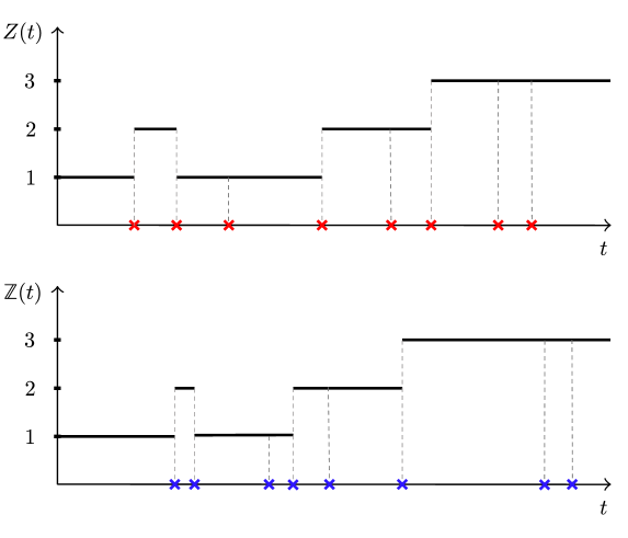
Refer to caption
Figure 3.1. Paths of the processes $Z$ and $\mathbb{Z}$ traversing the state space $\mathcal{J}=\{1,2,3\}$. Poissonian times of $\Gamma$ associated to $Z$ are shown with a red cross, while those of $\mathbb{\Gamma}$ associated to $\mathbb{Z}$ are shown with a blue cross. Note that $Z$ and $\mathbb{Z}$ sequentially visit the same states at the Poissonian epochs $\Gamma$ and $\mathbb{\Gamma}$.

However, since $\Gamma$ and $\mathbb{\Gamma}$ have identical distributional characteristics, we can expect their paths to be close to each other: we will investigate this statement in a precise way later in Theorem 3.2. Meanwhile, let us compute the distributional characteristics of the approximated process $\mathbb{Z}$ when conditioned on $\Gamma$. To do so, we first need to define an additional auxiliary process, $\mathbb{M}$, by letting

$$\beta_{0}=0,\quad\beta_{\ell+1}=\left\{\begin{array}[]{ccc}\beta_{\ell}+1&\mbox{if}&U(\chi_{\ell+1})\neq 0,\\ 0&\mbox{if}&U(\chi_{\ell+1})=0,\end{array}\right.$$
$$\mbox{and}\quad\mathbb{M}(s)=\beta_{\mathbb{\Gamma}(s)}.$$

In short, $\mathbb{M}$ is a process that jumps at the same epochs as $\mathbb{\Gamma}$, either increasing by $1$ or restarting at 00.

Theorem 3.1.

The process $(\mathbb{\Gamma},\mathbb{M},\mathbb{Z})$ with state space $\amsmathbb{N}_{0}\times\amsmathbb{N}_{0}\times\mathcal{J}$, when conditioned on $\Gamma$, is a time-homogeneous Markov jump process with random transition intensities given by

(3.8) $\displaystyle\Sigma(\ell_{1},w_{1},i_{1};\ell_{2},w_{2},i_{2})=\left\{\begin{array}[]{lll}\gamma\,Q_{i_{1},i_{2}}(\ell_{1},w_{1})&\mbox{if}&\begin{array}[]{l}\ell_{2}=\ell_{1}+1,w_{2}=0,i_{2}\neq i_{1},\;\mbox{or}\\ \ell_{2}=\ell_{1}+1,w_{2}=w_{1}+1,i_{2}=i_{1},\end{array}\\ 0&&\mbox{other }(\ell_{1},w_{1},i_{1})\neq(\ell_{2},w_{2},i_{2}),\\ -\gamma&&(\ell_{1},w_{1},i_{1})=(\ell_{2},w_{2},i_{2}).\end{array}\right.$

where

(3.9) $$\bm{Q}(\ell,w)=\bm{I}+\tfrac{1}{\gamma}\bm{\Lambda}(\chi_{\ell+1},\chi_{\ell+1}-\chi_{\ell-w})\quad\mbox{for}\quad\ell\geq w.$$
Proof.

We start by computing the law of the process $\{X_{\ell}\}_{\ell\geq 0}$ conditional on $\Gamma$, where $X_{\ell}:=(\beta_{\ell},\eta_{\ell})$. First,

$\displaystyle{\amsmathbb P}$ $\displaystyle(X_{\ell+1}=(w_{2},i_{2})\mid\Gamma,X_{0},X_{1},\dots,X_{\ell-1},X_{\ell}=(w_{1},i_{1}))$
$\displaystyle={\amsmathbb P}(X_{\ell+1}=(w_{2},i_{2})\mid\Gamma,X_{\ell}=(w_{1},i_{1})),$

where we implicitly used the strong Markov property for the process $\{t,U(t),Z(t)\}_{t\geq 0}$ at time $\chi_{\ell}$. Consequently, when conditioned on $\Gamma$, $\{X_{\ell}\}_{\ell\geq 0}$ is a (time-inhomogeneous) Markov chain. Now, note that the values for $\Gamma$ and $X_{\ell}$ characterize those of $\chi_{\ell+1}$ and $U(\chi_{\ell+1}-)$, the latter being

(3.10) $$U(\chi_{\ell+1}-)=\chi_{\ell+1}-\chi_{\ell-\beta_{\ell}}.$$

Using shorthand notation $\{\chi_{\ell+1}\in\Gamma_{0}\}$ for the event where the arrival $\chi_{\ell+1}$ is associated with $\Gamma_{0}$ (as opposed to $\Gamma^{\prime}$), then

$\displaystyle{\amsmathbb P}$ $\displaystyle(X_{\ell+1}=(w_{2},i_{2})\mid X_{\ell}=(w_{1},i_{1}),\chi_{\ell+1}=y,U(\chi_{\ell+1}-)=s)$
$\displaystyle={\amsmathbb P}(X_{\ell+1}=(w_{2},i_{2})\mid X_{\ell}=(w_{1},i_{1}),\chi_{\ell+1}=y,U(\chi_{\ell+1}-)=s,\chi_{\ell+1}\in\Gamma_{0}){\amsmathbb P}(\chi_{\ell+1}\in\Gamma_{0})$
$\displaystyle\quad+{\amsmathbb P}(X_{\ell+1}=(w_{2},i_{2})\mid X_{\ell}=(w_{1},i_{1}),\chi_{\ell+1}=y,U(\chi_{\ell+1}-)=s,\chi_{\ell+1}\notin\Gamma_{0}){\amsmathbb P}(\chi_{\ell+1}\notin\Gamma_{0})$
$\displaystyle=\left(\delta_{w_{1}+1,w_{2}}\delta_{i_{1},i_{2}}\left(1+\frac{\Lambda_{i_{1}i_{2}}(y,s)}{\gamma_{0}}\right)+\delta_{0,w_{2}}\delta_{i_{1},i_{2}}^{c}\left(\frac{\Lambda_{i_{1}i_{2}}(y,s)}{\gamma_{0}}\right)\right)\frac{\gamma_{0}}{\gamma}+\delta_{w_{1}+1,w_{2}}\delta_{i_{1},i_{2}}\frac{\gamma-\gamma_{0}}{\gamma}$
$\displaystyle=\delta_{w_{1}+1,w_{2}}\delta_{i_{1},i_{2}}+(\delta_{w_{1}+1,w_{2}}\delta_{i_{1},i_{2}}+\delta_{0,w_{2}}\delta_{i_{1},i_{2}}^{c})\left(\frac{\Lambda_{i_{1}i_{2}}(y,s)}{\gamma}\right),$

where $\delta_{i_{1},i_{2}}^{c}=1-\delta_{i_{1},i_{2}}$. Thus, employing (3.10), the transition probabilities of $\{X_{\ell}\}_{\ell\geq 0}$ conditional on $\Gamma$ are given by

$\displaystyle{\amsmathbb P}$ $\displaystyle(X_{\ell+1}=(w_{2},i_{2})\mid\Gamma,X_{\ell}=(w_{1},i_{1}))$
$\displaystyle=\delta_{w_{1}+1,w_{2}}\delta_{i_{1},i_{2}}+(\delta_{w_{1}+1,w_{2}}\delta_{i_{1},i_{2}}+\delta_{0,w_{2}}\delta_{i_{1},i_{2}}^{c})\left(\frac{\Lambda_{i_{1}i_{2}}(\chi_{\ell+1},\chi_{\ell+1}-\chi_{\ell-w_{1}})}{\gamma}\right)$

To “homogenize” the time-inhomogeneous Markov chain $\{X_{\ell}\}_{\ell\geq 0}$, we consider the augmented process $\{(\ell,\beta_{\ell},\eta_{\ell})\}_{\ell\geq 0}$, which is easily seen to follow the transition probabilities

$\displaystyle{\amsmathbb P}$ $\displaystyle((\ell+1,\beta_{\ell+1},\eta_{\ell+1})=(\ell_{2},w_{2},i_{2})\mid(\ell,\beta_{\ell},\eta_{\ell})=(\ell_{1},w_{1},i_{1}))$
(3.11) $\displaystyle=\delta_{\ell_{1}+1,\ell_{2}}{\amsmathbb P}(X_{\ell_{1}+1}=(w_{2},i_{2})\mid X_{\ell_{1}}=(w_{1},i_{1})).$

Applying the uniformization method (see e.g. [Van Dijk et al., 2018]) to the Markov chain $\{(\ell,\beta_{\ell},\eta_{\ell})\}_{\ell\geq 0}$ subordinated at the independent Poisson process $\mathbb{\Gamma}$ with intensity $\gamma$, yields the Markov jump process $\{(\mathbb{\Gamma}(s),\beta_{\mathbb{\Gamma}(s)},\eta_{\mathbb{\Gamma}(s)})\}_{s\geq 0}=(\mathbb{\Gamma},\mathbb{M},\mathbb{Z})$. The jump intensities of this process correspond to the product of the transition probabilities (3.11) with the intensity $\gamma$, which finally yields (3.8). ∎

Below, we state an important result that formally establishes $(\mathbb{Z},\mathbb{U})$, where $\mathbb{U}=\{\mathbb{U}(t)\}_{t\geq 0}$ is the duration process associated to $\mathbb{Z}$ via

(3.12) $$\mathbb{U}(t)=\inf\{r>0:\mathbb{Z}(t-r)\neq\mathbb{Z}(t)\},$$

as an appropriate approximation to the semi-Markov process $Z$. Its proof is included in the Appendix A.

Theorem 3.2.

$(\mathbb{Z},\mathbb{U})$ converges strongly to $(Z,U)$ in Skorokhod’s $J_{1}$-topology as $\gamma\rightarrow\infty$.

As discussed in [Prokhorov, 1956, Lemma 1.2], the almost sure $J_{1}$ convergence implies the convergence of the associated measures with respect to the Lévy-Prokhorov distance. In particular, this guarantees that the probability measure of the stochastic process $(\mathbb{Z},\mathbb{U})$ converges to that of $(Z,U)$. This result is significant as it not only ensures the convergence of their transition probabilities in a pointwise manner but also implies that the expectation of any bounded continuous functional evaluated at $\mathbb{Z}$ will converge to that of $Z$.

3.2. Efficient computation of the transition probabilities

In view of Theorem 3.2, we now use the process $(\mathbb{Z},\mathbb{U})$ to develop an approximating scheme for the transition probabilities of the original process $(Z,U)$. For $0\leq t\leq s$, $0\leq u\leq s$, and $0\leq v\leq t$, define the grid-conditional transition probabilities $\mathbb{p}(s,\mathrm{d}v)=\{\mathbb{p}_{ij}(s,\mathrm{d}v)\}_{i,j\in\mathcal{J}}$ where

$$\mathbb{p}_{ij}(s,v)={\amsmathbb P}(\mathbb{Z}(s)=j,\mathbb{U}(s)\leq v\mid\Gamma,\,\mathbb{Z}(0)=i,\,\mathbb{U}(0)=0).$$

Due to the doubly-infinite-dimensional structure of the state-space of $(\mathbb{\Gamma},\mathbb{M},\mathbb{Z})$, computing $\mathbb{p}_{ij}(s,\mathrm{d}v)$ via raw matrix-exponentiation using Theorem 3.1 is, in general, intractable. Below, we present a recursive algorithm that avoids this. In the following, $\mathrm{Poi}_{\lambda}(k)$ for $k\in\amsmathbb{N}_{0}$ takes the form $e^{-\lambda}(\lambda)^{k}/k!$, and $\mathrm{Erl}_{k,\lambda}(x)$ for $x\geq 0$ takes the form $\lambda(\lambda x)^{k-1}e^{-\lambda x}/(k-1)!$.

Theorem 3.3.

The measure $\mathbb{p}_{ij}(s,\mathrm{d}v)$ can be explicitly computed via

(3.13) $\displaystyle\mathbb{p}_{ij}(s,\mathrm{d}v)=\sum_{\ell,w\,:\,w\leq\ell}\mathbb{p}_{ij}(\ell,w;s,\mathrm{d}v).$

The summands consist of an atomic part at $v=s$ described by

(3.16) $\displaystyle\mathbb{p}_{ij}(\ell,w;s,\mathrm{d}v)$ $\displaystyle=\left\{\begin{array}[]{lll}\mathrm{Poi}_{\gamma s}(\ell)\times\Pi_{ii}(\ell,w)&\mbox{if}&i=j,\ell=w\geq 0\\ 0&&\mbox{otherwise},\end{array}\right.$

and an absolutely continuous part described by

(3.19) $\displaystyle\mathbb{p}_{ij}(\ell,w;s,\mathrm{d}v)$ $\displaystyle=\left\{\begin{array}[]{lll}\mathrm{Erl}_{\ell-w,\gamma}(s-v)\times\mathrm{Poi}_{\gamma v}(w)\times\Pi_{ij}(\ell,w)\mathrm{d}v&\mbox{if}&\ell>w\geq 0,v<s\\ 0&&\mbox{otherwise},\end{array}\right.$

where $\bm{\Pi}(\ell,w)=\{\Pi_{ij}(\ell,w)\}_{ij}$ may be computed via the recursion (3.20)-(3.23).

(3.20) $\displaystyle\bm{\Pi}(0,0)$ $\displaystyle=\bm{I}$
(3.21) $\displaystyle\bm{\Pi}(k,v)$ $\displaystyle=\bm{0}\quad\mbox{for all}\quad v>k$
(3.22) $\displaystyle\bm{\Pi}(k,0)$ $\displaystyle=\sum_{k^{\prime}=0}^{k-1}\bm{\Pi}(k-1,k^{\prime})\bm{Q}^{\mathrm{n}}(k-1,k^{\prime})\quad\mbox{for all}\quad k\geq 1$
(3.23) $\displaystyle\bm{\Pi}(k,v)$ $\displaystyle=\bm{\Pi}(k-1,v-1)\bm{Q}^{\mathrm{d}}(k-1,v-1)\quad\mbox{for all}\quad k\geq v\geq 1.$

Here,

$$\bm{Q}^{\mathrm{d}}(\ell,w)=\begin{pmatrix}Q_{11}(\ell,w)&&&\\ &Q_{22}(\ell,w)&&\\ &&\ddots&\\ &&&Q_{JJ}(\ell,w)\end{pmatrix}\quad\mbox{and}\quad\bm{Q}^{\mathrm{n}}(k,w)=\bm{Q}(k,w)-\bm{Q}^{\mathrm{d}}(k,w).$$
Proof.

Define where , follows the recursion Define the enlarged transition probabilities

$\displaystyle\mathbb{p}_{ij}$ $\displaystyle(\ell,w;s,\mathrm{d}v)={\amsmathbb P}(\mathbb{\Gamma}(s)=\ell,\mathbb{M}(s)=w,\mathbb{Z}(s)=j,\mathbb{U}(s)\in\mathrm{d}v\mid\Gamma,\,\mathbb{Z}(0)=i,\,\mathbb{U}(0)=0).$

By the law of total probability, it is clear that Equation 4.4 holds. Now, let $X_{k}=(\beta_{k},\eta_{k})$ be defined as in the proof of Theorem 3.1, and let

(3.24) $$\Pi_{ij}(\ell,w):={\amsmathbb P}(X_{\ell}=(w,j)\mid\Gamma,\,X_{0}=(0,i)),\quad\ell,w\geq 0;$$

in the following we relate $\Pi_{ij}(\ell,w)$ with $\mathbb{p}_{ij}(\ell,w;s,\mathrm{d}v)$, and show that it follows the recursion (3.20)-(3.23).

Case $v=s$. Under this event, $\mathbb{Z}$ does not change states in the interval $[0,s]$, so the only non-zero possibility is $i=j$ and $\ell=w$, which we study next. Equation (3.16) then follows by conditioning on the number of jumps of $\mathbb{\Gamma}$ in $[0,s]$, (which follows a probability mass function $\mathrm{Poi}_{\gamma s}(\ell)$) and multiplying by the grid-conditional probability of

$$\{X_{\ell^{\prime}}*\notin\{0\}\times\mathcal{J}\mbox{ and }\;X_{\ell^{\prime}}*\in\amsmathbb{N}_{0}\times\{i\}\mbox{ for all }1\leq\ell^{\prime}\leq\ell\;\}=\{X_{\ell}=(w,j)\},$$

where we employed that $\ell=w$ and thus $\eta_{0}=\eta_{1}=\cdots=\eta_{\ell}=i$.

Case $0<v<s$. In this event, a restart is bound to happen in $s-v\in[0,s]$, so the only non-zero case is when $\ell>w$. Furthermore, $\mathbb{\Gamma}(s-v-)\neq\mathbb{\Gamma}(s-v)=\ell-w$, $\mathbb{M}(s-v)=0$, and $\mathbb{Z}(s-v-)\neq\mathbb{Z}(s-v)=j$. After $s-v$, $\mathbb{Z}$ needs to remain in $j$ for $w$ incremental steps of $\mathbb{\Gamma}$ (or $\mathbb{M}$). In other words, by conditioning on the $(\ell-w)$th arrival of $\mathbb{\Gamma}$ at $s-v$ (which follows an $\mathrm{Erl}_{\ell-w,\gamma}(x)$) and on $w$ arrivals of $\mathbb{\Gamma}$ occurring in the interval $(s-v,s]$ (occurring with probability $\mathrm{Poi}_{\gamma v}(w)$), and multiplying by the grid-conditional probability of $\{X_{\ell}=(w,i)\}$ (event that captures the aforementioned dynamics), we obtain Equation (3.19).

We now discuss how the recursion (3.20)-(3.23) arises. Equation (3.20) is a straightforward initial condition, (3.21) describes the impossibility of having more arrivals associated with $\mathbb{M}$ than with $\mathbb{\Gamma}$. Concerning Equations (3.22) and (3.23), they are consequences of conditioning one step prior to $\ell$ (in terms of the process $\{X_{k}\}_{k\geq 0}$ in (3.24)) and employing the law of total probability. ∎

3.3. Value function evaluation

Now that we have a tractable expression for the grid-conditional transition probabilities of $(\mathbb{Z},\mathbb{U})$, we employ these to provide approximations to the value function $V(t;i,u)$. However, without loss of generality, we focus on obtaining approximations to $V_{k}:=V(0;i,0)$ only: time-shifting arguments akin to those presented in Subsection 2.2 yield the general case.

Thus, we define the grid-conditional approximation as

(3.25) $\displaystyle\mathbb{V}_{i}$ $\displaystyle=\amsmathbb{E}\left[\int_{0}^{T}e^{-\int_{t}^{s}r}\mathrm{d}\mathbb{B}(s)\mid\Gamma,\mathbb{Z}(t)=i,\mathbb{U}(t)=0\right],$
(3.26) $\displaystyle\mathrm{d}\mathbb{B}(t)$ $\displaystyle=\mathrm{d}B^{\mathbb{Z}(t),\mathbb{U}(t)}+\sum_{k\neq\mathbb{Z}(t-)}b^{(\mathbb{Z}(t-),\mathbb{U}(t-)),(k,0)}(t)\mathrm{d}\mathbb{N}^{k}(t),$
(3.27) $\displaystyle\mathbb{N}^{k}$ $\displaystyle=\sum_{s\in[0,t]}{\mathds{1}}\{\mathbb{Z}(s)=k,\mathbb{Z}(s-)\neq k\}.$

Based on our findings in Theorem 3.3, we now provide a remarkably tractable expression for $\mathbb{V}_{i}$.

Corollary 3.4.

For $i,j,k\in\mathcal{J}$,$j\neq k$ and $s\geq 0$, let

(3.28) $\displaystyle\mathbb{p}_{ij}(s,\mathrm{d}v)$ $\displaystyle=\mathbb{p}_{ij}^{\mathrm{a}}(s)\delta_{s}(v)+\mathbb{p}_{ij}^{\mathrm{c}}(s,v)\mathrm{d}v,$
(3.29) $\displaystyle\mathbb{p}_{i;jk}(s,\mathrm{d}v)$ $\displaystyle=\mathbb{p}_{i;jk}^{\mathrm{a}}(s)\delta_{s}(v)+\mathbb{p}_{i;jk}^{\mathrm{c}}(s,v)\mathrm{d}v,$

where

$\displaystyle\mathbb{p}_{ij}^{\mathrm{a}}(s)=\sum_{\ell\geq 0}\mathbb{p}_{ij}^{\mathrm{a}}(\ell;s),\qquad\mathbb{p}_{i;jk}^{\mathrm{a}}(s)=\sum_{\ell\geq 0}\mathbb{p}_{ij}^{\mathrm{a}}(\ell;s)(\gamma Q_{jk}(\ell,\ell)),$
$\displaystyle\mathbb{p}_{ij}^{\mathrm{c}}(s,v)=\sum_{\ell,w\,:\,w<\ell}\mathbb{p}_{ij}^{\mathrm{c}}(\ell,w;s,v),\qquad\mathbb{p}_{i;jk}^{\mathrm{c}}(s,v)=\sum_{\ell,w\,:\,w<\ell}\mathbb{p}_{ij}^{\mathrm{c}}(\ell,w;s,v)(\gamma Q_{jk}(\ell,w)),$
$\displaystyle\mathbb{p}_{ij}^{\mathrm{a}}(\ell;s)=\mathrm{Poi}_{\gamma s}(\ell)\;{\Pi}_{ii}(\ell,\ell)\;\mathds{1}_{\{i=j\}},$
$\displaystyle\mathbb{p}_{ij}^{\mathrm{c}}(\ell,w;s,v)=\mathrm{Erl}_{\ell-w,\gamma}(s-v)\;\mathrm{Poi}_{\gamma v}(w)\;{\Pi}_{ij}(\ell,w)\;\mathds{1}_{\{\ell>w\geq 0,v<s\}}.$

Then,

$\displaystyle\mathbb{V}_{i}$ $\displaystyle=\int_{s=0}^{T}e^{-\int_{0}^{s}r}\sum_{j\in\mathcal{J}}\int_{v=0}^{s}\mathbb{p}_{ij}(s,\mathrm{d}v)\mathrm{d}B^{j,v}(s)$
(3.30) $\displaystyle\qquad+\int_{s=0}^{T}e^{-\int_{0}^{s}r}\sum_{\begin{subarray}{c}j,k\in\mathcal{J}\\ j\neq k\end{subarray}}\int_{v=0}^{s}\mathbb{p}_{i;jk}(s,\mathrm{d}v)b^{(j,v),(k,0)}(s)\mathrm{d}s.$
Proof.

First, note that (3.28) is simply a re-statement of Theorem 3.3. The first summand in the r.h.s. of (3.30) follows by noting that

$\displaystyle\amsmathbb{E}\Big{(}\int_{0}^{T}e^{-\int_{t}^{s}r}\sum_{j\in\mathcal{J}}\mathds{1}_{\{\mathbb{Z}(t)=j\}}\mathrm{d}B^{j,\mathbb{U}(s)}(s)\;\Big{|}\;\Gamma,\mathbb{Z}(0)=i,\mathbb{U}(0)=0\Big{)}$
$\displaystyle\quad=\int_{0}^{T}e^{-\int_{t}^{s}r}\sum_{j\in\mathcal{J}}\amsmathbb{E}\left(\left.\mathds{1}_{\{\mathbb{Z}(t)=j\}}\mathrm{d}B^{j,\mathbb{U}(s)}(s)\;\right|\;\Gamma,\mathbb{Z}(0)=i,\mathbb{U}(0)=0\right)$
$\displaystyle\quad=\int^{T}_{s=0}e^{-\int_{0}^{s}r}\sum_{j\in\mathcal{J}}\int_{v=0}^{s}\mathbb{p}_{ij}(s,\mathrm{d}v)\mathrm{d}B^{j,v}(s).$

For the second summand, observe that for $j\neq k$,

$$\mathbb{N}_{jk}(t)=\sum_{\begin{subarray}{c}\ell,w\\ w\leq\ell\end{subarray}}\mathbb{N}_{jk;\ell,w}(t),$$

where $\mathbb{N}_{jk;\ell,w}$ represents the counting process linked to the jumps of $\mathbb{Z}$ from $j$ to $k$ occurring while $\mathbb{\Gamma}$ is $\ell$ and $\mathbb{M}$ is $w$ (before the jump). This counting process, $\mathbb{N}_{jk;\ell,w}$, has a jump intensity described by $\mathds{1}_{\mathbb{N}(s-)=\ell,\mathbb{M}(s-)=w,\mathbb{Z}(s-)=j}(\gamma Q_{jk}(\ell,w))$. By the general theory of counting processes (see [Asmussen and Steffensen, 2020] and more generally [Brémaud, 1981]) this leads to

$\displaystyle\amsmathbb{E}$ $\displaystyle\Big{(}\int_{0}^{T}e^{-\int_{t}^{s}r}\sum_{\begin{subarray}{c}j,k\in\mathcal{J}\\ j\neq k\end{subarray}}b^{(j,\mathbb{U}(s-)),(k,0)}(s)\,\mathrm{d}\mathbb{N}_{jk}(s)\;\Big{|}\;\Gamma,\mathbb{Z}(0)=i,\mathbb{U}(0)=0\Big{)}$
$\displaystyle\quad=\int_{0}^{T}e^{-\int_{t}^{s}r}\sum_{\begin{subarray}{c}j,k\in\mathcal{J}\\ j\neq k\end{subarray}}\sum_{\begin{subarray}{c}\ell,w\\ w\leq\ell\end{subarray}}\amsmathbb{E}\left(\left.b^{(j,\mathbb{U}(s-)),(k,0)}(s)\,\mathrm{d}\mathbb{N}_{jk;\ell,w}(s)\;\right|\;\Gamma,\mathbb{Z}(0)=i,\mathbb{U}(0)=0\right)$
$\displaystyle\quad=\int_{s=0}^{T}e^{-\int_{0}^{s}r}\sum_{\begin{subarray}{c}j,k\in\mathcal{J}\\ j\neq k\end{subarray}}\sum_{\begin{subarray}{c}\ell,w\\ w\leq\ell\end{subarray}}\int_{v=0}^{s}\mathbb{p}_{ij}(\ell,w;s,\mathrm{d}v)(\gamma Q^{\mathrm{n}}_{jk}(\ell,w))b^{(j,v),(k,0)}(s)\,\mathrm{d}s$
$\displaystyle\quad=\int_{s=0}^{T}e^{-\int_{0}^{s}r}\sum_{\begin{subarray}{c}j,k\in\mathcal{J}\\ ,j\neq k\end{subarray}}\int_{v=0}^{s}\mathbb{p}_{i;jk}(s,\mathrm{d}v)b^{(j,v),(k,0)}(s)\mathrm{d}s,$

where the final equality is a result of reorganizing the terms in (3.29).

To conclude this section, we emphasize that most of the results presented up to this point concern grid-conditional probabilities or expectations. While these hold under fairly robust assumptions, dealing with conditional quantities implies that the formulas are, in essence, random variables that converge to a constant when $\gamma\rightarrow\infty$. Although applying a Monte Carlo method would accelerate the convergence to the desired descriptor, this would inevitably require more computing power. In the next section, under certain regularity conditions, we provide an alternative approximation that circumvents the need for grid-conditional quantities and offers unconditional ones instead.

4. Unconditional approximations of semi-Markov processes

Note that the grid-conditional transition probabilities $\mathbb{p}_{ij}$ in Theorem 3.3 inherit their randomness from the matrices $\bm{Q}^{\mathrm{d}}(\ell,w)$ and $\bm{Q}^{\mathrm{n}}(\ell,w)$, themselves being defined through the matrix $\bm{Q}(\ell,w)=\bm{I}+\tfrac{1}{\gamma}\bm{\Lambda}(\chi_{\ell+1},\chi_{\ell+1}-\chi_{\ell-w})$. Here we propose to use the matrix $\widetilde{\bm{Q}}(\ell,w)$ instead of $\bm{Q}(\ell,w)$, where

(4.1) $\displaystyle\widetilde{\bm{Q}}(\ell,w)=\bm{I}+\tfrac{1}{\gamma}\bm{\Lambda}\left(\tfrac{\ell+1}{\gamma},\tfrac{w+1}{\gamma}\right).$

Note that we are effectivelly removing the randomess by replacing $\chi_{\ell+1}$ and $\chi_{\ell+1}-\chi_{\ell-w}$ with their expected values, $\tfrac{\ell+1}{\gamma}$ and $\frac{w+1}{\gamma}$. Heuristically, the strong law of large numbers implies that, indeed, each $\chi_{\ell}$ converges to their expected value. In fact, as evidenced by [Bladt and Peralta, 2022, Lemma 1, Eq (17)] – included here in the formula (B.9) of Appendix B – the stochastic grid $\Gamma=\{\chi_{\ell}\}_{\ell\geq 0}$ converges uniformly to the deterministic grid $\{\ell/\gamma\}_{\ell\geq 0}$ over increasing compact intervals. As expected, in order for $\widetilde{\bm{Q}}(\ell,w)$ to inherit this convergence, we need some type of continuity assumption for $\bm{\Lambda}$. In this section we we assume that $\bm{\Lambda}(s,v)=\{\Lambda_{ij}(s,v)\}$ is entrywise Lipschitz continuous, that is, there exists some $K>0$ such that

(4.2) $\displaystyle\left|\Lambda_{ij}(s_{1},v_{1})-\Lambda_{ij}(s_{2},v_{2})\right|\leq K\left(|s_{1}-s_{2}|+|v_{1}-v_{2}|\right).$

Under the assumption (4.2),

$\displaystyle\left|Q_{ij}(\ell,w)-\widetilde{Q}_{ij}(\ell,w)\right|$ $\displaystyle=\gamma^{-1}\left|\Lambda_{ij}(\chi_{\ell+1},\chi_{\ell+1}-\chi_{\ell-w})-\Lambda_{ij}\left(\tfrac{\ell+1}{\gamma},\tfrac{w+1}{\gamma}\right)\right|$
$\displaystyle\leq\gamma^{-1}K\left[\left|\chi_{\ell+1}-\tfrac{\ell+1}{\gamma}\right|+\left|\left(\chi_{\ell+1}-\chi_{\ell-w}\right)-\left(\tfrac{w+1}{\gamma}\right)\right|\right]$
$\displaystyle\leq\gamma^{-1}K\left[\left|\chi_{\ell+1}-\tfrac{\ell+1}{\gamma}\right|+\left|\left(\chi_{\ell+1}-\chi_{\ell-w}\right)-\left(\tfrac{\ell+1}{\gamma}-\tfrac{\ell-w}{\gamma}\right)\right|\right]$
$\displaystyle\leq\gamma^{-1}K\left[\left|\chi_{\ell+1}-\tfrac{\ell+1}{\gamma}\right|+\left|\chi_{\ell+1}-\tfrac{\ell+1}{\gamma}\right|+\left|\chi_{\ell-w}-\tfrac{\ell-w}{\gamma}\right|\right]$
(4.3) $\displaystyle\leq\gamma^{-1}3K\sup_{\ell^{\prime}\leq\ell+1}\left|\chi_{\ell}-\tfrac{\ell}{\gamma}\right|,$

confirming that $\widetilde{\bm{Q}}(\ell,w)$ converges to $\bm{Q}(\ell,w)$, at an $o(\gamma^{-1})$ rate, as long as the maximum distance between $\chi_{\ell^{\prime}}$ and $\ell^{\prime}/\gamma$ for all $\ell^{\prime}\leq\ell+1$ converges to 00, which is guaranteed by (B.9) of Appendix B.

The next step is identifying how the convergence of $\widetilde{\bm{Q}}(\ell,w)$ to $\bm{Q}(\ell,w)$ implies the convergence of the associated transition probabilities. For this, consider now a Markov chain $\{\widetilde{X}_{k}\}_{k\geq 0}$ over the state space $\amsmathbb{N}_{0}\times\mathcal{J}$ driven by the transition probabilities

$\displaystyle{\amsmathbb P}\left(\widetilde{X}_{k+1}=(w^{\prime},j)|\widetilde{X}_{k}=(w,i)\right)=\left\{\begin{array}[]{ccc}\widetilde{Q}^{\mathrm{d}}_{ii}(k,w)&\mbox{ if }&i=j,w^{\prime}=w+1\geq 1\\ \widetilde{Q}^{\mathrm{n}}_{ij}(k,w)&\mbox{ if }&i\neq j,w^{\prime}=0,w\geq 0\\ 0&&\mbox{otherwise},\end{array}\right.$

where

$$\widetilde{\bm{Q}}^{\mathrm{d}}(\ell,w)=\begin{pmatrix}\widetilde{Q}_{11}(\ell,w)&&&\\ &\widetilde{Q}_{22}(\ell,w)&&\\ &&\ddots&\\ &&&\widetilde{Q}_{JJ}(\ell,w)\end{pmatrix}\quad\mbox{and}\quad\widetilde{\bm{Q}}^{\mathrm{n}}(k,w)=\widetilde{\bm{Q}}(k,w)-\widetilde{\bm{Q}}^{\mathrm{d}}(k,w).$$

Now, we uniformize the three-dimensional process $\{(k,X_{k})\}_{k\geq 0}$ over a Poisson process $\widetilde{\mathbb{\Gamma}}$ of intensity $\gamma$, resulting in a continuous-time Markov jump process $(\widetilde{\mathbb{\Gamma}},\widetilde{\mathbb{M}},\widetilde{\mathbb{Z}})$. By arguments analogous to those presented in Theorem 3.3, we get that the associated transition probabilities. Specifically,

$$\widetilde{\mathbb{p}}_{ij}(s,v)={\amsmathbb P}(\widetilde{\mathbb{Z}}(s)=j,\widetilde{\mathbb{U}}(s)\leq v\mid\,\widetilde{\mathbb{Z}}(0)=i,\,\widetilde{\mathbb{U}}(0)=0)$$

with

$$\widetilde{\mathbb{U}}(t)=\inf\{r>0:\widetilde{\mathbb{Z}}(t-r)\neq\widetilde{\mathbb{Z}}(t)\},$$

can be computed via

(4.4) $\displaystyle\widetilde{\mathbb{p}}_{ij}(s,\mathrm{d}v)$ $\displaystyle=\widetilde{\mathbb{p}}_{ij}^{\mathrm{a}}(s)\delta_{s}(v)+\widetilde{\mathbb{p}}_{ij}^{\mathrm{c}}(s,v)\mathrm{d}v,$

where

$\displaystyle\widetilde{\mathbb{p}}_{ij}^{\mathrm{a}}(s)=\sum_{\ell\geq 0}\mathbb{p}_{ij}^{\mathrm{a}}(\ell;s),\quad\widetilde{\mathbb{p}}_{ij}^{\mathrm{c}}(s,v)=\sum_{\ell,w\,:\,w<\ell}\widetilde{\mathbb{p}}_{ij}^{\mathrm{c}}(\ell,w;s,v),$
$\displaystyle\widetilde{\mathbb{p}}_{ij}^{\mathrm{a}}(\ell;s)=\mathrm{Poi}_{\gamma s}(\ell)\;\widetilde{\Pi}_{ii}(\ell,\ell)\;\mathds{1}_{\{i=j\}},$
$\displaystyle\widetilde{\mathbb{p}}_{ij}^{\mathrm{c}}(\ell,w;s,v)=\mathrm{Erl}_{\ell-w,\gamma}(s-v)\;\mathrm{Poi}_{\gamma v}(w)\;\widetilde{\Pi}_{ij}(\ell,w)\;\mathds{1}_{\{\ell>w\geq 0,v<s\}}.$

Here $\widetilde{\bm{\Pi}}(\ell,w)=\{\widetilde{\Pi}_{ij}(\ell,w)\}_{ij}$ where

$\displaystyle\widetilde{\Pi}_{ij}(\ell,w):={\amsmathbb P}(\widetilde{X}_{\ell}=(w,j)\mid\widetilde{X}_{0}=(0,i)),\quad\ell,w\geq 0,$

follows the recursion

(4.5) $\displaystyle\widetilde{\bm{\Pi}}(0,0)$ $\displaystyle=\bm{I}$
(4.6) $\displaystyle\widetilde{\bm{\Pi}}(k,v)$ $\displaystyle=\bm{0}\quad\mbox{for all}\quad v>k$
(4.7) $\displaystyle\widetilde{\bm{\Pi}}(k,0)$ $\displaystyle=\sum_{k^{\prime}=0}^{k-1}\widetilde{\bm{\Pi}}(k-1,k^{\prime})\widetilde{\bm{Q}}^{\mathrm{n}}(k-1,k^{\prime})\quad\mbox{for all}\quad k\geq 1$
(4.8) $\displaystyle\widetilde{\bm{\Pi}}(k,v)$ $\displaystyle=\widetilde{\bm{\Pi}}(k-1,v-1)\widetilde{\bm{Q}}^{\mathrm{d}}(k-1,v-1)\quad\mbox{for all}\quad k\geq v\geq 1.$

Then we have the following convergence result regarding the densities associated to $\mathbb{p}_{ij}(\ell,w;s,\mathrm{d}v)$ and $\widetilde{\mathbb{p}}_{ij}(\ell,w;s,\mathrm{d}v)$; we include its proof in Appendix B.

Theorem 4.1.

For any $q>1$, $\varepsilon>0$, there exists a constant $\alpha(q,\varepsilon)$ such that for all $i,j\in J$ and $s\geq v\geq 0$,

$\displaystyle{\amsmathbb P}\left(\left|\mathbb{p}_{ij}^{\mathrm{a}}(s)-\widetilde{\mathbb{p}}_{ij}^{\mathrm{a}}(s)\right|\leq(s+1)\,\alpha(q,\varepsilon)\,(\log\gamma)\gamma^{-1/2+\varepsilon/2}\right)=o(\gamma^{-q}),$
$\displaystyle{\amsmathbb P}\left(\left|\int_{0}^{v}\mathbb{p}_{ij}^{\mathrm{c}}(s,v^{\prime})\mathrm{d}v^{\prime}-\int_{0}^{v}\widetilde{\mathbb{p}}_{ij}^{\mathrm{c}}(s,v^{\prime})\mathrm{d}v^{\prime}\right|\leq(s+1)\,\alpha(q,\varepsilon)\,(\log\gamma)\gamma^{-1/2+\varepsilon/2}\right)=o(\gamma^{-q}).$

Finally, having ensured that the unconditional transition probabilities converge to the same (almost sure) limit of the grid-conditional ones, and that this limit corresponds to the transition probabilities of the original process $(Z,U)$, we propose using the unconditional transition probabilities to approximate the value of $V_{i}$ in a manner akin to that of $\mathbb{V}_{i}$. Specifically, we consider the approximation $\widetilde{\mathbb{V}}_{i}$ where

$\displaystyle\widetilde{\mathbb{V}}_{i}$ $\displaystyle=\int_{s=0}^{T}e^{-\int_{0}^{s}r}\sum_{j\in\mathcal{J}}\int_{v=0}^{s}\widetilde{\mathbb{p}}_{ij}(s,\mathrm{d}v)\mathrm{d}B^{j,v}(s)$
$\displaystyle\qquad+\int_{s=0}^{T}e^{-\int_{0}^{s}r}\sum_{\begin{subarray}{c}j,k\in\mathcal{J}\\ j\neq k\end{subarray}}\int_{v=0}^{s}\widetilde{\mathbb{p}}_{i;jk}(s,\mathrm{d}v)b^{(j,v),(k,0)}(s)\mathrm{d}s,$

for $\widetilde{\mathbb{p}}_{ij}(s,\mathrm{d}v)$ defined as in (4.4), and

$\displaystyle\widetilde{\mathbb{p}}_{i;jk}(s,\mathrm{d}v)$ $\displaystyle=\widetilde{\mathbb{p}}_{i;jk}^{\mathrm{a}}(s)\delta_{s}(v)+\widetilde{\mathbb{p}}_{i;jk}^{\mathrm{c}}(s,v)\mathrm{d}v,$
$\displaystyle\widetilde{\mathbb{p}}_{i;jk}^{\mathrm{a}}(s)$ $\displaystyle=\sum_{\ell\geq 0}\widetilde{\mathbb{p}}_{ij}^{\mathrm{a}}(\ell;s)(\gamma\widetilde{Q}_{jk}(\ell,\ell)),$
$\displaystyle\widetilde{\mathbb{p}}_{i;jk}^{\mathrm{c}}(s,v)$ $\displaystyle=\sum_{\ell,w\,:\,w<\ell}\widetilde{\mathbb{p}}_{ij}^{\mathrm{c}}(\ell,w;s,v)(\gamma\widetilde{Q}_{jk}(\ell,w)).$

Note that the approximations $\mathbb{V}_{i}$ and $\widetilde{\mathbb{V}}_{i}$ are asymptotically equivalent and for small precision, virtually indistinguishable.

5. Illustration and extensions

This section illustrates the numerical feasibility of our methods. First we conduct the evaluation of cashflows (the main component of the value function) for a semi-Markov parametrization calibrated with real-life data. The emphasis is not that our method is more precise or faster than the state-of-the-art numerical integro-differential solvers, but instead that it is an extremely simple and straightforward algorithm which has very low chance of incurring in human error. Finally, we give a view towards credit risk and controlled semi-Markov models, as a potential use of our stochastic approximation.

5.1. Actuarial cashflows

Consider an actuarial application by analyzing the disability model with a semi-Markov structure, which is one of the most general stochastic structures implemented in the life-insurance market. This model considers three states: active, disabled, and dead, where all transitions are allowed except that, evidently, death is an absorbing state. The model is conceptually depicted in Figure 5.1.

active 00 dead $2$ disabled $1$ $\lambda_{12}(t)$ $\lambda_{23}(t)$ $\lambda_{13}(t)$ $\lambda_{23}(t)$
Figure 5.1. The disability model.

The main focus of an actuary is often not directly $\mathbb{V}_{i}$, but rather the following quantity referred to as the cashflow:

$\displaystyle\mathcal{C}_{i}(\mathrm{d}s)=\amsmathbb{E}\left[\mathrm{d}\mathbb{B}(s)\mid\Gamma,\mathbb{Z}(t)=i,\mathbb{U}(t)=0\right]$

which can be used by construct the value function $\mathbb{V}_{i}$. As the name indicates, the cashflow represents the instantaneous (and un-discounted) rate of payment transfer from the insurer to the insured. Premium payments may be included in this transfer, accounted as negative payments to the insured. The estimator of the cashflow using our strong approximation takes the form

$\displaystyle\mathbb{C}_{i}(s)$ $\displaystyle=\sum_{j\in\mathcal{J}}\int_{v=0}^{s}\mathbb{p}_{ij}(s,\mathrm{d}v)b^{j,v}(s)+\sum_{\begin{subarray}{c}j,k\in\mathcal{J}\\ j\neq k\end{subarray}}\int_{v=0}^{s}\mathbb{p}_{i;jk}(s,\mathrm{d}v)b^{(j,v),(k,0)}(s).$

where we have assumed for simplicity absolute continuity: $\mathrm{d}B^{j,v}(s)=b^{j,v}(s)\mathrm{d}s$. Now consider the following payment rules:

$\displaystyle b^{j,v}(s)$ $\displaystyle=1_{\{j=2\}}1_{\{v>1/10\}}\exp(-(s-v)/5),$
$\displaystyle b^{(j,v),(k,0)}(s)$ $\displaystyle=1_{\{j=1,k>1\}}+1_{\{j=2,k=3\}}.$

The first one states that there are only stream payments when in disability, and they only commence after having been a minimum time of $1/10$ time units in disability. The second states that lump-sum payments (of unit size) are possible only when deteriorating, that is from transitioning from active to disabled or dead, or when transitioning from disabled to dead.

Next, consider a semi-Markov structure for the underling jump-process, which is inspired by a calibration on real-life data from an undisclosed Danish life insurer. As stressed in the introduction, the fact that a Markov model is not sufficient to capture line insurance dynamics is well documented, and the internal calibration was done after exploring duration effects on the data with subsampling methods (cf. [Bladt and Furrer, 2023b] and the Vignette in the R package AalenJohansen [Bladt and Furrer, 2023a] for statistical non-parametric unveiling of duration effects from raw data). After unveiling non-Markovian effects, the final estimation is parametric, and uses a semi-Markov spline parametrization for the transition rates of the general likelihood formula of a jump-process, as provided in [Andersen et al., 2012].

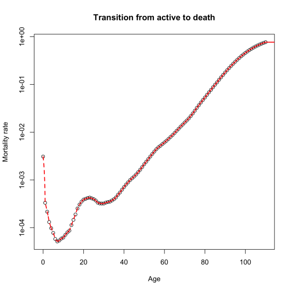
The transition rates are given as follows. The transition from active to death, given by $\lambda_{13}(t,u)$, is independent of duration and calibrated to mortality data through spline interpolation as shown in the top left panel of Figure 5.2.

Refer to caption
Refer to caption
Refer to caption
Refer to caption
Figure 5.2. Semi-Markov transition rates for life-insurance portfolio. Top left: mortality data and calibrated splines; top right: transition rate from active to disabled; bottom left: transitions from disabled to active; bottom right: transitions from disabled to death.

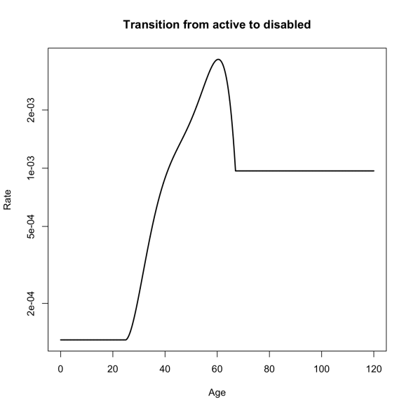
Transitions to disability are also duration independent, and calibrated internally, which provides the following estimate:
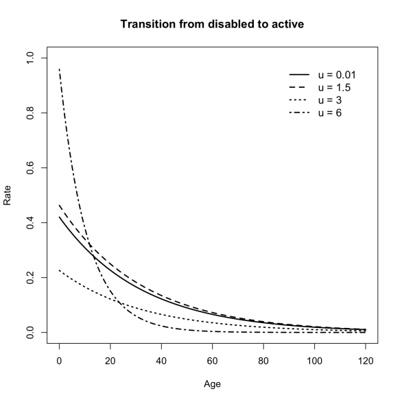
$\displaystyle\lambda_{12}(t,u)=\begin{cases}\lambda_{12,\text{base}}(25)&\text{if }t\leq 25\\ \lambda_{12,\text{base}}(t)&\text{if }25<t\leq 67\\ \lambda_{12,\text{base}}(67)&\text{if }t>67,\end{cases}$

where $\lambda_{12,\text{base}}(t)$ is the exponential of a fifth-order polynomial in $t$. A figure of $\lambda_{12}(t,u)$ as a function of $t$ (since it does not depend on $u$) is provided in the top right panel of Figure 5.2. Notice that before entering the workforce and after retirement age, the disability rate is constant, according to this model. The recovery rate is given by

$\displaystyle\lambda_{21}(t,u)=\begin{cases}\exp(\phi_{3}+\beta_{1}t+\theta_{3}u)&\text{if }u\leq 0.23\\ \exp(\phi_{2}+\beta_{1}t+\theta_{2}u)&\text{if }0.23<u\leq 2\\ \exp(\phi_{1}+\beta_{1}t+\theta_{1}u)&\text{if }2<u\leq 5\\ \exp(\phi_{0}+\beta_{2}t)&\text{if }u>5,\end{cases}$

for suitable parameters $\phi_{i},\beta_{i},\theta_{i}$. The bottom left panel of Figure 5.2 depicts the behaviour of the recovery rate as a function of $t$ for various fixed duration values $u$. We see that recovery does not improve with age, and duration also impacts recovery negatively for adults. Realistically, the rate is only precise for ages $25$ to $65$ since that is the range where most data lies in. Extrapolation into very young or very old ages is unreliable but also usually not required for practical purposes.

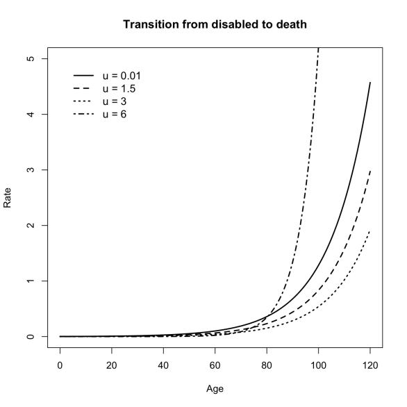
The only other rate that requires specification is mortality rate from disability, given by

$\displaystyle\lambda_{21}(t,u)=\begin{cases}\exp(\alpha_{1}+\eta_{1}t+\zeta_{1}u)&\text{if }u\leq 5\\ \exp(\alpha_{2}+\eta_{2}t)&\text{if }u>5\end{cases}$

for suitable $\alpha_{i},\eta_{i},\zeta_{i}$, and is depicted in the bottom right panel of Figure 5.2.

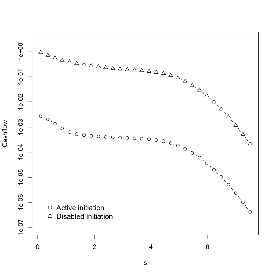
Finally, we compute the cashflow for the first two states, active and disabled, since the cashflow in the death state is clearly zero. The result of the approximation is shown in Figure 5.3. We would like to highlight that the implementation of the cashflow approximation formula is straightforward and can be evaluated efficiently using high-level programming languages, and circumvents not only user error but also numerical instability of integro-differential equation solvers.

Refer to caption
Figure 5.3. Approximation of the cashflow for the semi-Markov disability model over time.

5.2. Reduced form models for credit risk

In this section we suggest how our model could be extended for pricing defaultable claims (such as defaultable bonds, or Credit Default Swaps) in reduced form models. The classical martingale approach to asset pricing of [Harrison and Pliska, 1981, Harrison and Kreps, 1979] consists of taking an expectation under a risk neutral measure $\mathbb{Q}$, equivalent to the real-world probability measure $\mathbb{P}$, of a contingent claim, and discounted by the cumulative interest. When the claim is defaultable, in other words, there is a risk that it is not paid in full, then it was shown in [Duffie and Singleton, 1999, Collin-Dufresne et al., 2004] that valuation can proceed similarly, albeit with a discount factor that is default adjusted and under a risk neutral measure that is absolutely continuous with respect to $\mathbb{P}$ and not necessarily equivalent.

Consider a claim that pays a contingent payoff $X(T)$ at maturity $T$ in the case of no default. The default can be generic, either the default of the company as in the case of a defaultable bond, or it can be the default of a reference entity, in the case of Credit Default Swaps. Since the seminal paper of [Duffie and Singleton, 1999], closed form solutions can be provided under an assumption of zero recovery as

(5.1) $$V(t)=\amsmathbb{E}^{\mathbb{Q}}\left[e^{-\int_{t}^{T}(r_{s}+h_{s})ds}X(T)|\mathcal{F}_{t}\right],$$

where $r_{t}$ represents an interest rate and $h_{t}$ represents the default rate. This setup can be extended to case of a recovery that is a proportional to the market value, but for simplicity, we consider here the case of zero recovery rate. Our framework allows us to extend the classical valuation to the case of semi-Markov state-variable processes. As in the insurance setting, the credit risk model is driven by the state-variable process $Z=\{Z(t)\}_{t\geq 0}$ with duration process $U=\{U(t)\}_{0\leq t\leq T}$.

As in the classical credit risk setup of [Duffie and Singleton, 1999], we let $X(T)=\Phi(tTZ(T))$, for some function $\Phi$. The price at time $t$ of the defaultable claim becomes

$$V(t;i,u)=\amsmathbb{E}^{\mathbb{Q}}\left[e^{-\int_{t}^{T}(r_{s}+h_{s})ds}\Phi(Z(T))\mid Z(t)=i,U(t)=u\right],\quad i\in\mathcal{J},\>u\geq 0,$$

It is understood that in the semi-Markovian setup, the default rate $h_{t}$ depends on the duration as well. We can think it $h_{t}$ as an absorbing intensity, i.e., the transition rate to a cemetery state $\partial$ that represents the state of default,

(5.2) $$h_{t}=\lambda_{Z(t),\partial}(t,U(t)).$$

Note that this setup with state and duration dependent intensity, provides an alternative to existing credit risk models in the literature, mostly based on Markovian and affine state processes, see, e.g., [Duffie, 2004]. In contrast, here the state process $Z(t)$ is semi-Markovian, we have duration dependence, and the hazard function $\lambda$ is an arbitrary function that verifies the boundedness condition (for the grid-conditional approximation) and the Lipschitz continuity condition for the unconditional approximation. Note that the discount factor depends on the entire trajectory of the intensity process. We expect that our baseline setup can be extended to this type of valuation in order to achieve computational tractability.

5.3. Control

We now assume that that an agent can choose, at time 00, a control that depends on the time and duration process which affects the process $Z$ via its intensities. Under mild assumptions, our framework allows for such control. More specifically, for a set $\mathcal{A}$ of real measurable functions over $\mathds{R}_{+}^{2}$, the agent chooses some $a\in\mathcal{A}$ such that $Z$ is driven by $\bm{\Lambda}(s,v,a(s,v))$. For a fixed $a$, $\bm{\Lambda}(\cdot,\cdot,\cdot)$ is effectively only dependent on $s$ and $v$. The construction of such a process remains identical to that of Section 2.2. In fact, it results in a construction on the same probability space for all $a\in\mathcal{A}$. The conditional approximation remains exactly the same as well. For the unconditional version, the following conditions are necessary in order to retain the entry-wise Lipschitzness of intensity matrix

  • $\Lambda$ is bounded and Lipschitz continuous on its three entries,

  • The family $\mathcal{A}$ is uniformly bounded and uniformly Lipschitz continuous (with every element sharing the same Lipschitz constant).

Moreover, under such conditions, the family $\mathcal{A}$ is compact, and thus, an optimal control at time zero exists. Our work paves the way to efficiently compute approximations for value functions and optimize over the control policies at time zero.

It would be interesting to extend our setup to that of an intensity control problem, see [Bismut, 1975, Brémaud, 1981]. The goal is minimize a criterion of the type

$$\amsmathbb{E}^{\mathbb{Q}}\left[\int_{0}^{T}e^{-\int_{0}^{t}\rho_{s}ds}\phi(t,Z(t),U(t),\Lambda(t))dt+e^{-\int_{t}^{T}\rho_{s}ds}\Phi(T,Z_{T})\right],$$

for a running cost $\phi$ and a terminal cost $\Phi$. When the discount factor is given as a default adjusted discount of the previous section $\rho_{t}=\lambda_{Z(t),\partial}(t,U(t))$, this setup no longer falls under our framework and would necessitate an extension to discount factors that depend on the trajectory of the intensity. We further assume that the running cost depends on the jump intensity from the current state, i.e, $\phi(t,Z(t),U(t),\Lambda(t))=\phi(t,Z(t),U(t),\Lambda_{Z(t),\cdot}(t,U(t)))$ and we assume that $\phi$ is a strictly convex running cost. The optimal $V^{*}$ solves the following Hamilton-Jacobi-Bellman Equation

$\displaystyle 0=$ $\displaystyle\frac{\partial V^{*}(t,i,u)}{\partial t}+\frac{\partial V^{*}(t,i,u)}{\partial u}$
$\displaystyle+\inf_{\Lambda}(-\Lambda_{i,\partial}(t,u)V^{*}(t,i,u)+\sum_{j}\Lambda_{i,j}(t,u)[V^{*}(t,j,u)-V^{*}(t,i,u)]+\phi(t,i,u,\Lambda))$
$\displaystyle V^{*}(T,i,u)=\Phi(T,i)$

By discretizing time and using approximations of the value function (which can be computed at a given time $t$ for all $j$ and $u$ at once), the optimal solution $\Lambda^{*}(t,u)$ could be approximated by solving

$$\inf_{\Lambda}(-\Lambda_{i,\partial}(t,u))\mathbb{V}^{*}(t,i,u)+\sum_{j}\Lambda_{i,j}(t,u)[\mathbb{V}^{*}(t,j,u)-\mathbb{V}^{*}(t,i,u)]+\phi(t,i,u,\Lambda_{i,\cdot}(t,u)))$$

where we would replace the exact optimal solution $V^{*}$ by its approximation.

Note that this is a constrained optimization problem, since $\sum_{j}\Lambda_{i,j}=0$. Given the linear constraint, the problem have a unique solution for a variety of running cost functions, for example quadratic costs. We leave for future work the extension of our setup to the case where there is a dependence of discount factors on the trajectory of the intensity.

Appendix A Proof of Theorem 3.2

We present an extended version of the proof for strong convergence from [Bladt and Peralta, 2022], analyzed there for the simpler case of time-inhomogeneous Markov jump processes. Let us borrow the notation and concepts introduced in Section 3, here shown superindexed by the term $(\gamma)$ to make explicit their dependence on $\gamma$. In order to prove convergence in the $J_{1}$-topology over the space of $\mathcal{J}$-valued càdlàg functions, denoted by $\mathcal{D}(\mathds{R}_{+},\mathcal{J})$, it is sufficient to find a family $\{\Delta^{(\gamma)}\}_{\gamma}$ of random homoeomorphic functions over $\mathds{R}^{+}$, and an increasing sequence $\{c_{k}\}_{k\geq 1}$ with $c_{k}\uparrow\infty$, such that

(A.1) $\displaystyle\sup_{s\geq 0}|\Delta^{(\gamma)}(s)-s|$ $\displaystyle\rightarrow 0,$
(A.2) $\displaystyle\sum_{k=1}^{\infty}2^{-k}\times\mathds{1}\left\{\mathbb{Z}^{(\gamma)}\big{(}\Delta^{(\gamma)}(s)\big{)}\neq\,Z(s)\mbox{ for some }s\leq c_{k}\right\}$ $\displaystyle\rightarrow 0,$
(A.3) $\displaystyle\sum_{k=1}^{\infty}2^{-k}\left(\left(\sup_{s\leq c_{k}}\left|\mathbb{U}^{(\gamma)}\big{(}\Delta^{(\gamma)}(s)\big{)}-U(s)\right|\right)\wedge 1\right)$ $\displaystyle\rightarrow 0,$

in an almost sure sense as $\gamma\rightarrow\infty$. Heuristically speaking, the function $\Delta^{(\gamma)}$ acts as a time change that for increasing compact time intervals, “couples” the paths of $\mathbb{Z}^{(\gamma)}$ and $Z$, approximates those of $\mathbb{U}^{(\gamma)}$ to $U$, while $\Delta^{(\gamma)}$ converges uniformly to the identity function. In fact, in order to prove (A.1)-(A.3) for our choice of $\Delta^{(\gamma)}$, next we obtain explicit bounds for their rates of strong convergence.

Fix $\varepsilon>0$ and define

(A.7) $\displaystyle\Delta^{(\gamma)}(t)=\left\{\begin{array}[]{ccc}t\frac{\theta^{(\gamma)}_{1}}{\chi^{(\gamma)}_{1}}&\mbox{for}&t\in\left[0,\chi^{(\gamma)}_{1}\right)\\ \theta^{(\gamma)}_{\ell}+(t-\chi^{(\gamma)}_{\ell})\frac{\theta^{(\gamma)}_{\ell+1}-\theta^{(\gamma)}_{\ell}}{\chi^{(\gamma)}_{\ell+1}-\chi^{(\gamma)}_{\ell}}&\mbox{for}&t\in\left[\chi^{(\gamma)}_{\ell},\chi^{(\gamma)}_{\ell+1}\right),\,\ell<\lfloor\gamma^{1+\varepsilon}\rfloor\\ \theta^{(\gamma)}_{\lfloor\gamma^{1+\varepsilon}\rfloor}+(t-\chi^{(\gamma)}_{\lfloor\gamma^{1+\varepsilon}\rfloor})&\mbox{for}&t\in\left[\chi^{(\gamma)}_{\lfloor\gamma^{1+\varepsilon}\rfloor},\infty\right).\end{array}\right.$

The function $\Delta$ is, in essence, a piecewise linear function that maps the point $\chi^{(\gamma)}_{\ell}$ to $\theta^{(\gamma)}_{\ell}$ for all $\ell\leq\lfloor\gamma^{1+\varepsilon}\rfloor$, and increases linearly at a rate $1$ after $\chi^{(\gamma)}_{\lfloor\gamma^{1+\varepsilon}\rfloor}$. Particularly, this implies that

(A.8) $$\mathbb{Z}^{(\gamma)}(\Delta^{(\gamma)}(s))=Z(s)\mbox{ for all }s\in\left[0,\chi^{(\gamma)}_{\lfloor\gamma^{1+\varepsilon}\rfloor}\right).$$

Furthermore, it can be readily verified that

(A.9) $$\sup_{s\geq 0}|\Delta^{(\gamma)}(s)-s|=\max_{\ell\in\{1,2,\dots,\lfloor\gamma^{1+\varepsilon}\rfloor\}}\left|\chi^{(\gamma)}_{\ell}-\theta^{(\gamma)}_{\ell}\right|.$$

Employing [Bladt and Peralta, 2022, Lemma 1], we arrive to

(A.10) $$\mathds{P}\left(\sup_{s\geq 0}|\Delta^{(\gamma)}(s)-s|\geq\alpha(\log\gamma)\gamma^{-1/2+\varepsilon/2}\right)=o(\gamma^{q}),$$

where $q$ is any arbitrary positive real number and $\alpha$ is a constant that only depends on $\varepsilon$ and $q$. Via standard Borell-Cantelli arguments (e.g., choosing $q=2$), it is straightforward to get (A.1) from (A.9).

For (A.2), note that due to (A.8),

$\displaystyle\sum_{k=1}^{\infty}2^{-k}\times\mathds{1}\left\{\mathbb{Z}^{(\gamma)}\big{(}\Delta^{(\gamma)}(s)\big{)}\neq\,Z(s)\mbox{ for some }s\leq c_{k}\right\}$
$\displaystyle\quad\leq\sum_{k=1}^{\infty}2^{-k}\times\mathds{1}\left\{\chi^{(\gamma)}_{\lfloor\gamma^{1+\varepsilon}\rfloor}\leq c_{k}\right\}$
$\displaystyle\quad=\sum_{k=1}^{\lfloor\gamma^{\varepsilon}\rfloor}2^{-k}\times\mathds{1}\left\{\chi^{(\gamma)}_{\lfloor\gamma^{1+\varepsilon}\rfloor}\leq c_{k}\right\}+\sum_{k=\lfloor\gamma^{\varepsilon}\rfloor+1}^{\infty}2^{-k}\times\mathds{1}\left\{\chi^{(\gamma)}_{\lfloor\gamma^{1+\varepsilon}\rfloor}\leq c_{k}\right\}$
(A.11) $\displaystyle\quad\leq\mathds{1}\left\{\chi^{(\gamma)}_{\lfloor\gamma^{1+\varepsilon}\rfloor}\leq c_{\lfloor\gamma^{\varepsilon}\rfloor}\right\}+2^{-\lfloor\gamma^{\varepsilon}\rfloor},$

where in the last inequality we used that $\{c_{k}\}_{k}$ is a (yet to be determined) increasing sequence. Since $2^{-\lfloor\gamma^{\varepsilon}\rfloor}\rightarrow 0$, then (A.2) will follow from (A.11) once we find a sequence $\{c_{k}\}_{k}$ such that $\mathds{1}\left\{\chi^{(\gamma)}_{\lfloor\gamma^{1+\varepsilon}\rfloor}\leq c_{\lfloor\gamma^{\varepsilon}\rfloor}\right\}\rightarrow 0$ almost surely. We claim that $c_{k}=k/2$ exhibits the desired property. Indeed, for this choice of $c_{k}$,

(A.12) $\displaystyle\left\{\chi^{(\gamma)}_{\lfloor\gamma^{1+\varepsilon}\rfloor}\leq c_{\lfloor\gamma^{\varepsilon}\rfloor}\right\}=\left\{\chi^{(\gamma)}_{\lfloor\gamma^{1+\varepsilon}\rfloor}\leq\frac{\lfloor\gamma^{\varepsilon}\rfloor}{2}\right\}=\left\{\frac{\gamma}{\lfloor\gamma^{1+\varepsilon}\rfloor}\chi^{(\gamma)}_{\lfloor\gamma^{1+\varepsilon}\rfloor}\leq\frac{\gamma}{\lfloor\gamma^{1+\varepsilon}\rfloor}\frac{\lfloor\gamma^{\varepsilon}\rfloor}{2}\right\}.$

The term $\frac{\gamma}{\lfloor\gamma^{1+\varepsilon}\rfloor}\chi^{(\gamma)}_{\lfloor\gamma^{1+\varepsilon}\rfloor}$ converges to 1 almost surely. This convergence can be verified by interpreting the term as the sum of $\lfloor\gamma^{1+\varepsilon}\rfloor$ i.i.d. exponential r.v.’s of parameter 1 scaled by the number of summands and then applying the SLLN. Additionally, the term $\frac{\gamma}{\lfloor\gamma^{1+\varepsilon}\rfloor}\frac{\lfloor\gamma^{\varepsilon}\rfloor}{2}$ converges to $\frac{1}{2}$. Given these convergences, (A.12) represents an asymptotically null set, and thus, (A.2) follows.

Finally, for (A.3), employing similar inequalities that lead to (A.11), we get

$\displaystyle\sum_{k=1}^{\infty}2^{-k}\left(\left(\sup_{s\leq c_{k}}\left|\mathbb{U}^{(\gamma)}\big{(}\Delta^{(\gamma)}(s)\big{)}-U(s)\right|\right)\wedge 1\right)$
$\displaystyle\quad\leq\left(\left(\sup_{s\leq c_{\lfloor\gamma^{\varepsilon}\rfloor}}\left|\mathbb{U}^{(\gamma)}\big{(}\Delta^{(\gamma)}(s)\big{)}-U(s)\right|\right)\wedge 1\right)+2^{-\lfloor\gamma^{\varepsilon}\rfloor}$
(A.13) $\displaystyle\quad\leq\left(\left(\sup_{s<\chi^{(\gamma)}_{\lfloor\gamma^{1+\varepsilon}\rfloor}}\left|\mathbb{U}^{(\gamma)}\big{(}\Delta^{(\gamma)}(s)\big{)}-U(s)\right|\right)\wedge 1\right)+\mathds{1}\left\{\chi^{(\gamma)}_{\lfloor\gamma^{1+\varepsilon}\rfloor}\leq c_{\lfloor\gamma^{\varepsilon}\rfloor}\right\}+2^{-\lfloor\gamma^{\varepsilon}\rfloor}.$

The almost sure convergence of the last two summands of (A.13) to zero were confirmed via (A.12). What remains is the almost sure convergence of the first summand of (A.13) to zero: establishing this will prove (A.3).

Let $\{\sigma^{(\gamma)}_{\ell}\}_{\ell}$ be the successive epochs at which $U$ returns to 00. Note that $U$ evolves like the identity function with a space translation to 00 at the time epochs $\{\sigma^{(\gamma)}_{\ell}\}_{\ell}$. Similarly, on the time interval $[0,\chi^{(\gamma)}_{\lfloor\gamma^{1+\varepsilon}\rfloor})$, $\mathbb{U}^{(\gamma)}\circ\Delta^{(\gamma)}$ evolves $\Delta^{(\gamma)}$ with a space-translation to 00 at the time epochs $\{\sigma^{(\gamma)}_{\ell}\}_{\ell}$. Thus, for $s\in[\sigma^{(\gamma)}_{\ell},\sigma^{(\gamma)}_{\ell+1})$,

$\displaystyle\left|\mathbb{U}^{(\gamma)}\big{(}\Delta^{(\gamma)}(s)\big{)}-U(s)\right|$
$\displaystyle\quad=\left|\mathbb{U}^{(\gamma)}\big{(}\Delta^{(\gamma)}(s)\big{)}-U(s)+\left(\Delta^{(\gamma)}(\sigma^{(\gamma)}_{\ell})-\sigma^{(\gamma)}_{\ell}\right)-\left(\Delta^{(\gamma)}(\sigma^{(\gamma)}_{\ell})-\sigma^{(\gamma)}_{\ell}\right)\right|$
$\displaystyle\quad\leq\left|\left(\mathbb{U}^{(\gamma)}\big{(}\Delta^{(\gamma)}(s)\big{)}+\Delta^{(\gamma)}(\sigma^{(\gamma)}_{\ell})\right)-\left(U(s)+\sigma^{(\gamma)}_{\ell}\right)\right|+\left|\Delta^{(\gamma)}(\sigma^{(\gamma)}_{\ell})-\sigma^{(\gamma)}_{\ell}\right|$
$\displaystyle\quad=\left|\Delta^{(\gamma)}(s)-s\right|+\left|\Delta^{(\gamma)}(\sigma^{(\gamma)}_{\ell})-\sigma^{(\gamma)}_{\ell}\right|.$

From this, it follows

(A.14) $\displaystyle\sup_{s<\chi^{(\gamma)}_{\lfloor\gamma^{1+\varepsilon}\rfloor}}\left|\mathbb{U}^{(\gamma)}\big{(}\Delta^{(\gamma)}(s)\big{)}-U(s)\right|\leq 2\times\sup_{s\geq 0}\left|\Delta^{(\gamma)}(s)-s\right|.$

This asserts the almost sure convergence of the l.h.s. of (A.14) to 00, as supported by (A.1). Consequently, (A.3) is derived, completing the proof.

Appendix B Proof of Theorem 4.1

Before we prove Theorem 4.1, we first present a couple of technical matrix-analytic results, namely, Lemma B.1 and Lemma B.2 below.

For any real matrices or vectors $\bm{A}^{(1)}=\{A_{ij}^{(1)}\}_{i,j}$ and $\bm{A}^{(2)}=\{A_{ij}^{(2)}\}_{i,j}$ of the same dimensions, we denote by $\bm{A}^{(1)}\leq\bm{A}^{(2)}$ the case for which $A_{ij}^{(1)}\leq A_{ij}^{(2)}$ for all $i,j$. Moreover, for a real matrix or vector $\bm{A}=\{A_{ij}\}_{i,j}$, define $|\bm{A}|$ to be the matrix whose entries correspond to the absolute values of those of $\bm{A}$. In particular, if $\bm{e}$ is a column-vector of ones of appropriate size, then

$$(|\bm{A}|\bm{e})_{j}=\sum_{k}|A_{jk}|\quad\text{for all }j.$$

Essentially, $|\bm{A}|\bm{e}$ corresponds to a column-vector form of the $\ell_{1}$-norm over the rows of $\bm{A}$. Some straightforward properties follow:

  • $\bm{0}\leq|\bm{A}|\bm{e}$ where $\bm{0}$ is a column-vector of zeroes of appropriate size,

  • $|\bm{A}^{(1)}+\bm{A}^{(2)}|\bm{e}\leq|\bm{A}^{(1)}|\bm{e}+|\bm{A}^{(2)}|\bm{e}$ for all matrices $\bm{A}^{(1)}$ and $\bm{A}^{(2)}$ of the same dimensions, with equality if each entry of $\bm{A}^{(1)}$ and $\bm{A}^{(2)}$ is not simultaneously non-zero for both matrices,

  • $|\bm{A}^{(1)}\bm{A}^{(2)}|\leq|\bm{A}^{(1)}||\bm{A}^{(2)}|$ for all square matrices $\bm{A}^{(1)}$ and $\bm{A}^{(2)}$ of the same dimensions,

  • $|c\bm{A}|\bm{e}=|\bm{A}|(c\bm{e})=c|\bm{A}|\bm{e}$ for all $c\geq 0$.

Lemma B.1.

Let $\bm{\Pi}$ be defined through the recursive Equations 3.20-3.23, and $\widetilde{\bm{\Pi}}$ through the recursive Equations 4.5-4.8. Then, for all $k\geq 0$ and $S\subseteq\{0,1,2,\dots k\}$,

(B.1) $\displaystyle\sum_{k^{\prime}\in S}\left|{\bm{\Pi}}(k,k^{\prime})-\widetilde{\bm{\Pi}}(k,k^{\prime})\right|\bm{e}\leq k\,C_{k}\,\bm{e},$

where $C_{0}=0$ and for $k\geq 1$,

(B.2) $\displaystyle C_{k}=\sup\left\{\left(\left|\bm{Q}(\ell,w)-\widetilde{\bm{Q}}(\ell,w)\right|\bm{e}\right)_{j}:0\leq w\leq\ell\leq k-1,\,j\in\mathcal{J}\right\}.$
Proof.

We proceed using induction over $k$. It is trivial to verify (B.1) for $k=0$. Suppose that (B.1) holds for $k-1\geq 0$, where the sum in the l.h.s. is taken over any subset of $\{0,1,2,\dots k-1\}$. For the induction step at $k$, fix some $S\subseteq\{0,1,2,\dots k\}$ and consider two cases.

Case $\{0\}\notin S$. Here,

$\displaystyle\sum_{k^{\prime}\in S}$ $\displaystyle\left|{\bm{\Pi}}(k,k^{\prime})-\widetilde{\bm{\Pi}}(k,k^{\prime})\right|\bm{e}$
$\displaystyle=\sum_{k^{\prime}\in S}\left|{\bm{\Pi}}(k-1,k^{\prime}-1){\bm{Q}}^{\mathrm{d}}(k-1,k^{\prime}-1)-\widetilde{\bm{\Pi}}(k-1,k^{\prime}-1)\widetilde{\bm{Q}}^{\mathrm{d}}(k-1,k^{\prime}-1)\right|\bm{e}$
$\displaystyle\leq\sum_{k^{\prime}\in S}\left|{\bm{\Pi}}(k-1,k^{\prime}-1)\left[{\bm{Q}}^{\mathrm{d}}(k-1,k^{\prime}-1)-\widetilde{\bm{Q}}^{\mathrm{d}}(k-1,k^{\prime}-1)\right]\right|\bm{e}$
$\displaystyle\qquad\qquad+\sum_{k^{\prime}\in S}\left|\left[{\bm{\Pi}}(k-1,k^{\prime}-1)-\widetilde{\bm{\Pi}}(k-1,k^{\prime}-1)\right]\widetilde{\bm{Q}}^{\mathrm{d}}(k-1,k^{\prime}-1)\right|\bm{e}$
$\displaystyle\leq\sum_{k^{\prime}\in S}\left|{\bm{\Pi}}(k-1,k^{\prime}-1)\right|\left|{\bm{Q}}^{\mathrm{d}}(k-1,k^{\prime}-1)-\widetilde{\bm{Q}}^{\mathrm{d}}(k-1,k^{\prime}-1)\right|\bm{e}$
$\displaystyle\qquad\qquad+\sum_{k^{\prime}\in S}\left|{\bm{\Pi}}(k-1,k^{\prime}-1)-\widetilde{\bm{\Pi}}(k-1,k^{\prime}-1)\right|\left|\widetilde{\bm{Q}}^{\mathrm{d}}(k-1,k^{\prime}-1)\right|\bm{e}$
(B.3) $\displaystyle\leq C_{k}\sum_{k^{\prime}\in S}\left|{\bm{\Pi}}(k-1,k^{\prime}-1)\right|\bm{e}+\sum_{k^{\prime}\in S}\left|{\bm{\Pi}}(k-1,k^{\prime}-1)-\widetilde{\bm{\Pi}}(k-1,k^{\prime}-1)\right|\bm{e}$
(B.4) $\displaystyle\leq C_{k}\,\bm{e}+(k-1)\,C_{k-1}\,\bm{e}\leq k\,C_{k}\,\bm{e},$

where in (B.3) we employed

$$\begin{gathered}|{\bm{Q}}^{\mathrm{d}}(k-1,k^{\prime}-1)-\widetilde{\bm{Q}}^{\mathrm{d}}(k-1,k^{\prime}-1)|\bm{e}\leq C_{k}\,\bm{e}\quad\mbox{and}\\ |\widetilde{\bm{Q}}^{\mathrm{d}}(k-1,k^{\prime}-1)|\bm{e}\leq\widetilde{\bm{Q}}(k-1,k^{\prime}-1)\bm{e}\leq\bm{e},\end{gathered}$$

and in (B.4) we used

$\displaystyle\sum_{k^{\prime}\in S}(\left|{\bm{\Pi}}(k-1,k^{\prime}-1)\right|\bm{e})_{i}$ $\displaystyle=\sum_{k^{\prime}\in S}\sum_{j}\Pi_{ij}(k-1,k^{\prime}-1)\leq 1,$

along with the induction step. Thus, (B.1) follows.

Case $\{0\}\in S$. In this scenario,

$\displaystyle\sum_{k^{\prime}\in S}\left|{\bm{\Pi}}(k,k^{\prime})-\widetilde{\bm{\Pi}}(k,k^{\prime})\right|\bm{e}$
$\displaystyle=\sum_{k^{\prime}\in S\backslash\{0\}}\left|{\bm{\Pi}}(k-1,k^{\prime}-1){\bm{Q}}^{\mathrm{d}}(k-1,k^{\prime}-1)-\widetilde{\bm{\Pi}}(k-1,k^{\prime}-1)\widetilde{\bm{Q}}^{\mathrm{d}}(k-1,k^{\prime}-1)\right|\bm{e}$
$\displaystyle\quad+\left|\sum_{k^{\prime}=0}^{k-1}{\bm{\Pi}}(k-1,k^{\prime}){\bm{Q}}^{\mathrm{n}}(k-1,k^{\prime})-\sum_{k^{\prime}=0}^{k-1}\widetilde{\bm{\Pi}}(k-1,k^{\prime})\widetilde{\bm{Q}}^{\mathrm{n}}(k-1,k^{\prime})\right|\bm{e}$
$\displaystyle\leq\sum_{k^{\prime}\in S\backslash\{0\}}\left|{\bm{\Pi}}(k-1,k^{\prime}-1){\bm{Q}}^{\mathrm{d}}(k-1,k^{\prime}-1)-\widetilde{\bm{\Pi}}(k-1,k^{\prime}-1)\widetilde{\bm{Q}}^{\mathrm{d}}(k-1,k^{\prime}-1)\right|\bm{e}$
$\displaystyle\quad+\sum_{k^{\prime}=0}^{k-1}\left|{\bm{\Pi}}(k-1,k^{\prime}){\bm{Q}}^{\mathrm{n}}(k-1,k^{\prime})-\widetilde{\bm{\Pi}}(k-1,k^{\prime})\widetilde{\bm{Q}}^{\mathrm{n}}(k-1,k^{\prime})\right|\bm{e}$
$\displaystyle\leq\sum_{k^{\prime}\in S\setminus\{0\}}\left|{\bm{\Pi}}(k-1,k^{\prime}-1)\right|\;\left|{\bm{Q}}^{\mathrm{d}}(k-1,k^{\prime}-1)-\widetilde{\bm{Q}}^{\mathrm{d}}(k-1,k^{\prime}-1)\right|\bm{e}$
$\displaystyle\quad+\sum_{k^{\prime}\in S\setminus\{0\}}\left|{\bm{\Pi}}(k-1,k^{\prime}-1)-\widetilde{\bm{\Pi}}(k-1,k^{\prime}-1)\right|\;\left|\widetilde{\bm{Q}}^{\mathrm{d}}(k-1,k^{\prime}-1)\right|\bm{e}$
$\displaystyle\quad+\sum_{k^{\prime\prime}=0}^{k-1}\left|{\bm{\Pi}}(k-1,k^{\prime\prime})\right|\;\left|{\bm{Q}}^{\mathrm{n}}(k-1,k^{\prime\prime})-\widetilde{\bm{Q}}^{\mathrm{n}}(k-1,k^{\prime\prime}-1)\right|\bm{e}$
$\displaystyle\quad+\sum_{k^{\prime\prime}=0}^{k-1}\left|{\bm{\Pi}}(k-1,k^{\prime\prime})-\widetilde{\bm{\Pi}}(k-1,k^{\prime\prime})\right|\;\left|\widetilde{\bm{Q}}^{\mathrm{n}}(k-1,k^{\prime\prime})\right|\bm{e},$

where in the last inequality we employed similar steps akin to those taken for the case $\{0\}\notin S$. Since ${\bm{Q}}^{\mathrm{d}}$ and ${\bm{Q}}^{\mathrm{n}}$ have entries which are not simultaneously non-zero (ditto $\widetilde{\bm{Q}}^{\mathrm{d}}$ and $\widetilde{\bm{Q}}^{\mathrm{n}}$), then the last inequality is equal to

$\displaystyle\sum_{k^{\prime\prime}=0}^{k-1}\left|{\bm{\Pi}}(k-1,k^{\prime\prime})\right|\;\left|\left({\bm{Q}}^{\mathrm{d}}(k-1,k^{\prime\prime})-\widetilde{\bm{Q}}^{\mathrm{d}}(k-1,k^{\prime\prime})\right)\mathds{1}_{k^{\prime\prime}+1\in\mathcal{S}}+\left({\bm{Q}}^{\mathrm{n}}(k-1,k^{\prime\prime})-\widetilde{\bm{Q}}^{\ {n}}(k-1,k^{\prime\prime})\right)\right|\bm{e}$
$\displaystyle\quad+\sum_{k^{\prime\prime}\in S\setminus\{0\}}\left|{\bm{\Pi}}(k-1,k^{\prime\prime})-\widetilde{\bm{\Pi}}(k-1,k^{\prime\prime})\right|\;\left|\widetilde{\bm{Q}}^{\mathrm{d}}(k-1,k^{\prime\prime})\mathds{1}_{k^{\prime\prime}+1\in\mathcal{S}}+\widetilde{\bm{Q}}^{\mathrm{n}}(k-1,k^{\prime\prime})\right|\bm{e}$
(B.5) $\displaystyle\leq C_{k}\sum_{k^{\prime\prime}=0}^{k-1}\left|{\bm{\Pi}}(k-1,k^{\prime\prime})\right|\bm{e}+\sum_{k^{\prime\prime}=0}^{k-1}\left|{\bm{\Pi}}(k-1,k^{\prime\prime})-\widetilde{\bm{\Pi}}(k-1,k^{\prime\prime})\right|\bm{e}$
(B.6) $\displaystyle\leq C_{k}\,\bm{e}+(k-1)\,C_{k-1}\,\bm{e}\leq k\,C_{k}\,\bm{e},$

where in (B.5) and (B.6) we employed

$$\begin{gathered}\left|({\bm{Q}}^{\mathrm{d}}(k-1,k^{\prime\prime})-\widetilde{\bm{Q}}^{\mathrm{d}}(k-1,k^{\prime\prime}))\mathds{1}_{k^{\prime\prime}+1\in\mathcal{S}}+({\bm{Q}}^{\mathrm{n}}(k-1,k^{\prime\prime})-\widetilde{\bm{Q}}^{\mathrm{n}}(k-1,k^{\prime\prime}))\right|\bm{e}\leq C_{k}\,\bm{e},\\ \left|\widetilde{\bm{Q}}^{\mathrm{d}}(k-1,k^{\prime\prime})\mathds{1}_{k^{\prime\prime}+1\in\mathcal{S}}+\widetilde{\bm{Q}}^{\mathrm{n}}(k-1,k^{\prime\prime})\right|\bm{e}\leq\widetilde{\bm{Q}}(k-1,k^{\prime\prime})\,\bm{e}\leq\bm{e},\\ \sum_{k^{\prime\prime}=0}^{k-1}(\left|{\bm{\Pi}}(k-1,k^{\prime\prime})\right|\bm{e})_{i}\leq 1,\end{gathered}$$

along with the induction hypothesis. Hence, (B.1) holds. ∎

Lemma B.2.

Let $C_{k}$ be defined by (B.2) and suppose that the Lipschitz condition (4.2) holds. Fix $q>1$ and $\varepsilon\in(0,1)$. Then, there exists $\beta(q,\varepsilon)$ such that

(B.7) $\displaystyle{\amsmathbb P}\left(C_{\lfloor\gamma^{1+\varepsilon}\rfloor}\geq\beta(q,\varepsilon)\,(\log\gamma)\,\gamma^{-3/2+\varepsilon/2}\right)=o(\gamma^{-q}).$
Proof.

From (4.3),

$\displaystyle C_{\lfloor\gamma^{1+\varepsilon}\rfloor}$ $\displaystyle=\sup\left\{\sum_{j^{\prime}}\left|Q_{jj^{\prime}}(\ell,w)-\widetilde{Q}_{jj^{\prime}}(\ell,w)\right|:0\leq w\leq\ell\leq\lfloor\gamma^{1+\varepsilon}\rfloor-1,\,j\in\mathcal{J}\right\}$
$\displaystyle=J\times\sup\left\{\left|Q_{jj^{\prime}}(\ell,w)-\widetilde{Q}_{jj^{\prime}}(\ell,w)\right|:0\leq w\leq\ell\leq\lfloor\gamma^{1+\varepsilon}\rfloor-1,\,j,j^{\prime}\in\mathcal{J}\right\}$
(B.8) $\displaystyle\leq 3JK\gamma^{-1}\sup_{\ell^{\prime}\leq{\lfloor\gamma^{1+\varepsilon}\rfloor}}\left|\chi_{\ell}-\tfrac{\ell}{\gamma}\right|.$

In [Bladt and Peralta, 2022, Lemma 1, Eq (17)] it is proved that

(B.9) $\displaystyle{\amsmathbb P}\left(\sup_{\ell^{\prime}\leq{\lfloor\gamma^{1+\varepsilon}\rfloor}}\left|\chi_{\ell}-\tfrac{\ell}{\gamma}\right|\geq\left(2\,e^{1/2+\varepsilon/2+2q}\right)\,(\log\gamma)\,\gamma^{-1/2+\varepsilon/2}\right)=o(\gamma^{-q}),$

which via (B.8), implies (B.7) with $\beta(q,\varepsilon)=6JKe^{1/2+\varepsilon/2+2q}$. ∎

Proof of Theorem 4.1..

For $s\geq 0$ and $i=j$, employing the triangle inequality, (B.1) and $\sum_{\ell\geq 0}\ell\,\mathrm{Poi}_{\gamma s}(\ell)=\gamma s$,

$\displaystyle\left|\mathbb{p}_{ij}^{\mathrm{a}}(s)-\widetilde{\mathbb{p}}_{ii}^{\mathrm{a}}(s)\right|$ $\displaystyle\leq\sum_{\ell\geq 0}\left|\mathbb{p}_{ij}^{\mathrm{a}}(\ell;s)-\widetilde{\mathbb{p}}_{ij}^{\mathrm{a}}(\ell;s)\right|$
$\displaystyle\leq\sum_{\ell\geq 0}\mathrm{Poi}_{\gamma s}(\ell)\;\left|{\Pi}_{ii}(\ell,\ell)-\widetilde{\Pi}_{ii}(\ell,\ell)\right|$
$\displaystyle\leq\sum_{0\leq\ell\leq\lfloor\gamma^{1+\varepsilon}\rfloor}\mathrm{Poi}_{\gamma s}(\ell)\;\left|{\Pi}_{ii}(\ell,\ell)-\widetilde{\Pi}_{ii}(\ell,\ell)\right|$
$\displaystyle\qquad+\sum_{\ell\geq\lfloor\gamma^{1+\varepsilon}\rfloor+1}\mathrm{Poi}_{\gamma s}(\ell)\left({\Pi}_{ii}(\ell,\ell)+\widetilde{\Pi}_{ii}(\ell,\ell)\right)$
$\displaystyle\leq\sum_{0\leq\ell\leq\lfloor\gamma^{1+\varepsilon}\rfloor}\mathrm{Poi}_{\gamma s}(\ell)\,\ell\,C_{\ell}+2\sum_{\ell\geq\lfloor\gamma^{1+\varepsilon}\rfloor+1}\mathrm{Poi}_{\gamma s}(\ell)$
$\displaystyle\leq C_{\lfloor\gamma^{1+\varepsilon}\rfloor}\sum_{0\leq\ell\leq\lfloor\gamma^{1+\varepsilon}\rfloor}\ell\,\mathrm{Poi}_{\gamma s}(\ell)+2\sum_{\ell\geq\lfloor\gamma^{1+\varepsilon}\rfloor+1}\mathrm{Poi}_{\gamma s}(\ell)$
$\displaystyle\leq C_{\lfloor\gamma^{1+\varepsilon}\rfloor}\sum_{\ell\geq 0}\ell\,\mathrm{Poi}_{\gamma s}(\ell)+2\sum_{\ell\geq\lfloor\gamma^{1+\varepsilon}\rfloor+1}\mathrm{Poi}_{\gamma s}(\ell)$
$\displaystyle\leq C_{\lfloor\gamma^{1+\varepsilon}\rfloor}(\gamma s)+2\sum_{\ell\geq\lfloor\gamma^{1+\varepsilon}\rfloor+1}\mathrm{Poi}_{\gamma s}(\ell).$

Similarly, for $0\leq v\leq s$ and $i,j\in\mathcal{J}$,

$\displaystyle\left|\int_{0}^{v}\mathbb{p}_{ij}^{\mathrm{c}}(s,v^{\prime})\mathrm{d}v^{\prime}-\int_{0}^{v}\widetilde{\mathbb{p}}_{ij}^{\mathrm{c}}(s,v^{\prime})\mathrm{d}v^{\prime}\right|\leq\int_{0}^{s}\left|\mathbb{p}_{ij}^{\mathrm{c}}(s,v^{\prime})-\widetilde{\mathbb{p}}_{ij}^{\mathrm{c}}(s,v^{\prime})\right|\mathrm{d}v^{\prime}$
$\displaystyle\quad\leq\int_{0}^{s}\sum_{\ell\geq 1}\sum_{w=0}^{\ell-1}\mathrm{Erl}_{\ell-w,\gamma}(s-v^{\prime})\;\mathrm{Poi}_{\gamma v^{\prime}}(w)\;\left|{\Pi}_{ij}(\ell,w)-\widetilde{\Pi}_{ij}(\ell,w)\right|\mathrm{d}v^{\prime}$
$\displaystyle\quad=\sum_{\ell\geq 1}\sum_{w=0}^{\ell-1}\left(\int_{0}^{s}\mathrm{Erl}_{\ell-w,\gamma}(s-v^{\prime})\;\mathrm{Poi}_{\gamma v^{\prime}}(w)\mathrm{d}v^{\prime}\right)\;\left|{\Pi}_{ij}(\ell,w)-\widetilde{\Pi}_{ij}(\ell,w)\right|$
$\displaystyle\quad=\sum_{\ell\geq 1}\mathrm{Poi}_{\gamma s}(\ell)\sum_{w=0}^{\ell-1}\left|{\Pi}_{ij}(\ell,w)-\widetilde{\Pi}_{ij}(\ell,w)\right|$
$\displaystyle\quad\leq\sum_{1\leq\ell\leq\lfloor\gamma^{1+\varepsilon}\rfloor}\mathrm{Poi}_{\gamma s}(\ell)\sum_{w=0}^{\ell-1}\left|{\Pi}_{ij}(\ell,w)-\widetilde{\Pi}_{ij}(\ell,w)\right|$
$\displaystyle\qquad\quad+\sum_{\ell\geq\lfloor\gamma^{1+\varepsilon}\rfloor+1}\mathrm{Poi}_{\gamma s}(\ell)\left(\sum_{w=0}^{\ell-1}{\Pi}_{ij}(\ell,w)+\sum_{w=0}^{\ell-1}\widetilde{\Pi}_{ij}(\ell,w)\right)$
$\displaystyle\quad\leq\sum_{1\leq\ell\leq\lfloor\gamma^{1+\varepsilon}\rfloor}\mathrm{Poi}_{\gamma s}(\ell)\,\ell\,C_{\ell}+2\sum_{\ell\geq\lfloor\gamma^{1+\varepsilon}\rfloor+1}\mathrm{Poi}_{\gamma s}(\ell)$
$\displaystyle\quad=C_{\lfloor\gamma^{1+\varepsilon}\rfloor}(\gamma s)+2\sum_{\ell\geq\lfloor\gamma^{1+\varepsilon}\rfloor+1}\mathrm{Poi}_{\gamma s}(\ell);$

note that we employed the identity $\int_{0}^{s}\mathrm{Erl}_{\ell-w,\gamma}(s-v^{\prime})\;\mathrm{Poi}_{\gamma v^{\prime}}(w)\mathrm{d}v^{\prime}=\mathrm{Poi}_{\gamma s}(\ell)$. In short, both $\left|\mathbb{p}_{ij}^{\mathrm{a}}(s)-\widetilde{\mathbb{p}}_{ii}^{\mathrm{a}}(s)\right|$ and $\left|\int_{0}^{v}\mathbb{p}_{ij}^{\mathrm{c}}(s,v^{\prime})\mathrm{d}v^{\prime}-\int_{0}^{v}\widetilde{\mathbb{p}}_{ij}^{\mathrm{c}}(s,v^{\prime})\mathrm{d}v^{\prime}\right|$ are bounded by

$$C_{\lfloor\gamma^{1+\varepsilon}\rfloor}(\gamma s)+2\sum_{\ell\geq\lfloor\gamma^{1+\varepsilon}\rfloor+1}\mathrm{Poi}_{\gamma s}(\ell)=C_{\lfloor\gamma^{1+\varepsilon}\rfloor}(\gamma s)+2{\amsmathbb P}(\chi_{\lfloor\gamma^{1+\varepsilon}\rfloor+1}<s).$$

The proof can then be concluded by noting that

$\displaystyle{\amsmathbb P}$ $\displaystyle\left(C_{\lfloor\gamma^{1+\varepsilon}\rfloor}(\gamma s)+2{\amsmathbb P}(\chi_{\lfloor\gamma^{1+\varepsilon}\rfloor+1}\geq(s+1)\,\alpha(q,\varepsilon)\,(\log\gamma)\gamma^{-1/2+\varepsilon/2})\right)$
$\displaystyle\leq{\amsmathbb P}\left(C_{\lfloor\gamma^{1+\varepsilon}\rfloor}(\gamma s)\geq s\,\alpha(q,\varepsilon)\,(\log\gamma)\gamma^{-1/2+\varepsilon/2})\right)$
$\displaystyle\quad+\mathds{1}\{2{\amsmathbb P}(\chi_{\lfloor\gamma^{1+\varepsilon}\rfloor+1}\leq s)\geq\alpha(q,\varepsilon)\,(\log\gamma)\gamma^{-1/2+\varepsilon/2}\}$
$\displaystyle={\amsmathbb P}\left(C_{\lfloor\gamma^{1+\varepsilon}\rfloor}\geq\alpha(q,\varepsilon)\,(\log\gamma)\gamma^{-3/2+\varepsilon/2})\right)$
$\displaystyle\quad+\mathds{1}\{2{\amsmathbb P}(\chi_{\lfloor\gamma^{1+\varepsilon}\rfloor+1}\leq s)\geq\alpha(q,\varepsilon)\,(\log\gamma)\gamma^{-1/2+\varepsilon/2}\}=o(\gamma^{-q}),$

where in the last step we employed (B.7) and the fact that ${\amsmathbb P}(\chi_{\lfloor\gamma^{1+\varepsilon}\rfloor+1}\leq s)$ decays at a $q^{\prime}$-polynomial rate for any $q^{\prime}>0$ (cf. (B.9)). ∎

Acknowledgement. MB and OP would like to acknowledge financial support from the Swiss National Science Foundation Project 200021_191984. AM and OP were partially supported by an AXA Research grant on Mitigating risk in the wake of the Covid-19 Pandemic.

Declaration We declare no conflict of interest related to the current manuscript.

References

  • [Ahmad et al., 2023] Ahmad, J., Bladt, M., and Bladt, M. (2023). Estimating absorption time distributions of general Markov jump processes. Scandinavian Journal of Statistics, pages 1–30.
  • [Andersen et al., 2012] Andersen, P. K., Borgan, O., Gill, R. D., and Keiding, N. (2012). Statistical models based on counting processes. Springer Science & Business Media.
  • [Asmussen and Steffensen, 2020] Asmussen, S. and Steffensen, M. (2020). Risk and insurance. Springer.
  • [Bismut, 1975] Bismut, J. (1975). Contrôle des processus de sauts. C. R. Acad. Sci. Paris Sér. A-B, 281(18):767–770.
  • [Bladt and Furrer, 2023a] Bladt, M. and Furrer, C. (2023a). AalenJohansen: Conditional Aalen-Johansen Estimation. R package version 1.0.
  • [Bladt and Furrer, 2023b] Bladt, M. and Furrer, C. (2023b). Conditional Aalen–Johansen estimation. arXiv:2303.02119. Under review, University of Copenhagen.
  • [Bladt and Peralta, 2022] Bladt, M. and Peralta, O. (2022). Strongly convergent homogeneous approximations to inhomogeneous Markov jump processes and applications. Under review, University of Lausanne.
  • [Brémaud, 1981] Brémaud, P. (1981). Point processes and queues. Springer.
  • [Buchardt et al., 2015] Buchardt, K., Møller, T., and Schmidt, K. B. (2015). Cash flows and policyholder behaviour in the semi-markov life insurance setup. Scandinavian Actuarial Journal, 2015(8):660–688.
  • [Cairns et al., 2008] Cairns, A. J., Blake, D., and Dowd, K. (2008). Modelling and management of mortality risk: a review. Scandinavian Actuarial Journal, 2008(2-3):79–113.
  • [Cinlar, 1969] Cinlar, E. (1969). Markov renewal theory. Advances in Applied Probability, 1(2):123–187.
  • [Collin-Dufresne et al., 2004] Collin-Dufresne, P., Goldstein, R., and Hugonnier, J. (2004). A general formula for valuing defaultable securities. Econometrica, 72(5):1377–1407.
  • [Duffie, 2004] Duffie, D. (2004). Credit risk modeling with affine processes. Scuola normale superiore.
  • [Duffie and Singleton, 1999] Duffie, D. and Singleton, K. J. (1999). Modeling term structures of defaultable bonds. The review of financial studies, 12(4):687–720.
  • [Fox and Glynn, 1986] Fox, B. L. and Glynn, P. W. (1986). Discrete-time conversion for simulating semi-markov processes. Operations Research Letters, 5(4):191–196.
  • [Harrison and Kreps, 1979] Harrison, J. M. and Kreps, D. M. (1979). Martingales and arbitrage in multiperiod securities markets. Journal of Economic theory, 20(3):381–408.
  • [Harrison and Pliska, 1981] Harrison, J. M. and Pliska, S. R. (1981). Martingales and stochastic integrals in the theory of continuous trading. Stochastic processes and their applications, 11(3):215–260.
  • [Hickman, 1964] Hickman, J. C. (1964). A statistical approach to premiums and reserves in multiple decrement theory. Transactions of the Society of Actuaries, 16(45):149–154.
  • [Hoem, 1969] Hoem, J. M. (1969). Markov chain models in life insurance. Blätter der DGVFM, 9(2):91–107.
  • [Hoem, 1972] Hoem, J. M. (1972). Inhomogeneous semi-markov processes, select actuarial tables, and duration-dependence in demography. In Population dynamics, pages 251–296. Elsevier.
  • [Janssen, 1966] Janssen, J. (1966). Application des processus semi-markoviens à un probléme d’invalidité. Bulletin de l’Association Royale des Actuaries Belges, 63:35–52.
  • [Janssen and De Dominicis, 1984] Janssen, J. and De Dominicis, R. (1984). Finite non-homogeneous semi-markov processes: Theoretical and computational aspects. Insurance: Mathematics and Economics, 3(3):157–165.
  • [Jensen, 1953] Jensen, A. (1953). Markoff chains as an aid in the study of markoff processes. Scandinavian Actuarial Journal, 1953(sup1):87–91.
  • [Lévy, 1954] Lévy, P. (1954). Processus semi-markoviens. In Proc. Int. Congress. Math. III, Amsterdam, 1954.
  • [Massey and Whitt, 1998] Massey, W. A. and Whitt, W. (1998). Uniform acceleration expansions for markov chains with time-varying rates. Annals of Applied Probability, pages 1130–1155.
  • [Prokhorov, 1956] Prokhorov, Y. V. (1956). Convergence of random processes and limit theorems in probability theory. Theory of Probability & Its Applications, 1(2):157–214.
  • [Smith, 1955] Smith, W. L. (1955). Regenerative stochastic processes. Proceedings of the Royal Society of London. Series A. Mathematical and Physical Sciences, 232(1188):6–31.
  • [Steffensen, 2006] Steffensen, M. (2006). Surplus-linked life insurance. Scandinavian Actuarial Journal, 2006(1):1–22.
  • [Sverdrup, 1952] Sverdrup, E. (1952). Basic concepts in life assurance mathematics. Scandinavian Actuarial Journal, 1952(3-4):115–131.
  • [Van Dijk, 1992] Van Dijk, N. M. (1992). Uniformization for nonhomogeneous markov chains. Operations research letters, 12(5):283–291.
  • [Van Dijk et al., 2018] Van Dijk, N. M., Van Brummelen, S. P. J., and Boucherie, R. J. (2018). Uniformization: Basics, extensions and applications. Performance evaluation, 118:8–32.