Mixture-of-Linear-Experts for Long-term Time Series Forecasting
 

Abstract

Long-term time series forecasting (LTSF) aims to predict future values of a time series given the past values. The current state-of-the-art (SOTA) on this problem is attained in some cases by linear-centric models, which primarily feature a linear mapping layer. However, due to their inherent simplicity, they are not able to adapt their prediction rules to periodic changes in time series patterns. To address this challenge, we propose a Mixture-of-Experts-style augmentation for linear-centric models and propose Mixture-of-Linear-Experts (MoLE). Instead of training a single model, MoLE trains multiple linear-centric models (i.e., experts) and a router model that weighs and mixes their outputs. While the entire framework is trained end-to-end, each expert learns to specialize in a specific temporal pattern, and the router model learns to compose the experts adaptively. Experiments show that MoLE reduces forecasting error of linear-centric models, including DLinear, RLinear, and RMLP, in over 78% of the datasets and settings we evaluated. By using MoLE existing linear-centric models can achieve SOTA LTSF results in 68% of the experiments that PatchTST reports and we compare to, whereas existing single-head linear-centric models achieve SOTA results in only 25% of cases. Additionally, MoLE models achieve SOTA in all settings for the newly released Weather2K datasets.

1 Introduction

Long-term time series forecasting (LTSF) is an important problem in the machine learning community, given its application in areas like weather modeling (Zhu et al., 2023; Wu et al., 2023), traffic flow prediction (Jiang et al., 2023), and financial forecasting (Ariyo et al., 2014).

Various classical methods (BOX, 1976; Fildes, 1991; Han et al., 2019) and deep-learning methods (Bai et al., 2018; Borovykh et al., 2017; Lai et al., 2018; Chang et al., 2018; Fan et al., 2019) have been used for this task, including transformers (Zhou et al., 2021; Wu et al., 2021; Zhang and Yan, 2022; Nie et al., 2022). However, recent studies show that in some settings, linear-centric models surpass prior baselines—including transformers—sometimes by a significant margin (Zeng et al., 2023; Li et al., 2023). Linear-centric models feature a single linear layer, possibly combined with non-linear pre- and postprocessing steps. Examples include DLinear, NLinear (Zeng et al., 2023), RLinear, and RMLP (Li et al., 2023).

However, real-world time series are usually non-stationary. For example, traffic patterns change on different days of the week. Due to the inherent simplicity of linear-centric models, it is difficult for them to capture these patterns.

In this paper, we propose Mixture-of-Linear-Experts (MoLE) to address the above limitation. We propose to train multiple linear-centric models (i.e., experts) to collaboratively predict the time series. A router model, which accepts a timestamp embedding of the input sequence as input, learns to weigh these experts adaptively. This layer is supposed to learn the periodicity of the time series and adjust the weights for each expert accordingly, ensuring that different experts specialize in different periods of the time series. Note that MoLE can be applied to any linear-centric model as-is.

More broadly, Mixture-of-Experts (MoE) has a long history (Jordan and Jacobs, 1994; Yuksel et al., 2012) and was recently revived due to its successful application in SOTA language (Artetxe et al., 2021; Yi et al., 2023; Shen et al., 2023) and image models (Riquelme et al., 2021; Dryden and Hoefler, 2022). Its main motivation in these domains has been efficiency: it increases model capacity without much inference overhead by training multiple experts simultaneously and only activating a subset of experts for a given input (a.k.a. Sparse Mixture-of-Experts (Shazeer et al., 2017)). In contrast, we show that MoE over linear-centric models gives significant gains in forecasting fidelity; MoLE keeps the simplicity of linear-centric models while using MoE to model diverse temporal patterns.

Our primary contributions include:

• We propose MoLE, a mixture-of-experts approach that can augment any linear-centric LTSF model to capture non-stationary temporal patterns.

• We demonstrate through comprehensive empirical evaluations that MoLE consistently improves upon existing linear-centric methods, including those that are currently SOTA for the LTSF problem. Concretely, we observe when MoLE was applied to DLinear, it enhanced its performance in 32/44 experimental settings (73% of experiments). Similarly, with the RLinear and RMLP models, integrating MoLE resulted in improvements in 38/44 scenarios (86%) and 33/44 scenarios (75%) respectively. We find that among the 28 datasets and settings that PatchTST reports and we compare to, MoLE allows linear-centric models to achieve SOTA results in 19 cases (68%), whereas without MoLE (single-head), they are SOTA in 7 settings (25%). For the Weather2K datasets, MoLE-linear-centric models achieve SOTA in all settings.

• We conduct careful ablation studies to explain the reasons for the success of MoLE; these show that the observed performance boost is due to the specialized time-aware experts rather than just an expanded model size. Moreover, the gains of MoLE are more pronounced when input sequence lengths are short compared to the prediction sequence length.

In all, MoLE offers an efficient and simple enhancement for linear-centric LTSF models, which can be used out-of-the-box for improved forecasting.

2 Related Work

We highlight three categories of LSTF models: those based on transformers, linear-centric models, and models based on other architectures.

Transformer-based models

Transformers have shown great potential and excellent performance in long-term time series forecasting (Zhou et al., 2021; Wu et al., 2021; Zhang and Yan, 2022; Wen et al., 2022). The first well-known transformer for LTSF, Informer (Zhou et al., 2021), addresses issues like quadratic time complexity with ProbSparse self-attention and a generative style decoder. Following Informer, models such as Autoformer (Wu et al., 2021), Pyraformer (Liu et al., 2021), Preformer (Du et al., 2023), and FEDFormer (Zhou et al., 2022a) were introduced. Autoformer (Wu et al., 2021) uses decomposition and auto-correlation for performance, Pyraformer (Liu et al., 2021) focuses on multiresolution attention for signal processing efficiency, Preformer (Du et al., 2023) introduces segment-wise correlation for efficient attention calculation, and FEDFormer (Zhou et al., 2022a) combines frequency analysis with Transformers for enhanced time series representation. The state-of-the-art model, PatchTST (Nie et al., 2022), shifts focus to the importance of patches, enhancing the model’s capability to capture local and global dependencies in data. We compare against PatchTST (Nie et al., 2022) as a SOTA transformer-based baseline.

Linear-centric models

Despite the success of transformer-based models in LTSF, Zeng et al. (2023) raised doubts about their efficacy. They proposed three linear or linear-centric models: vanilla linear, DLinear, and NLinear, which outperform existing transformer-based models by a large margin. Among the three models, DLinear is most commonly compared to in subsequent work (Nie et al., 2022; Li et al., 2023). We include DLinear as a baseline model that can be integrated with MoLE.

Following the work of Zeng et al. (2023), several other linear-centric models have been proposed (Li et al., 2023; Xu et al., 2023). We compare against RLinear and RMLP (Li et al., 2023) as the only linear-centric models that outperform PatchTST (Nie et al., 2022) on some datasets and settings.

Other architectures

Other common LTSF models are based on multi-layer perceptrons (MLP) (Wang et al., 2023b; Zhou et al., 2022b; Zhang et al., 2022; Shao et al., 2022; Chen et al., 2023; Das et al., 2023) and convolutional neural networks (CNN) (Wang et al., 2022, 2023a; Gong et al., 2023). Since these models are not directly evaluated in papers focusing on linear-centric and transformer-based models, we have not included them in our evaluation. The main point of this work is not to compare linear-centric models to transformers, but to propose a technique that improves linear centric-models.

Gruver et al. (2023) recently introduced the LLMTime model, which uses large language models as a zero-shot time series predictor. We were unable to compare to this model due to the high volume and prohibitive cost of API calls to proprietary LLMs. Their quantitative results also did not include exact numbers, but were listed as bar charts, so we could not compare against reported results either.

3 Preliminaries

3.1 Problem Definition

Time Series Forecasting

Given an input sequence $\mathbf{X}\in\mathbb{R}^{c\times s}$, where $c$ represents the number of channels (features) and $s$ denotes the number of historical (input) timestamps, our objective is to find a mapping $f(\mathbf{X})=\mathbf{Y}$ such that $\mathbf{Y}\in\mathbb{R}^{c\times p}$ and $p$ represents the number of future (output) timestamps to predict. Additionally, we are provided with the dates and times corresponding to each timestamp of $\mathbf{X}$ and $\mathbf{Y}$, represented as $\bm{x}_{mark}\in\mathbb{R}^{s}$ and $\bm{y}_{mark}\in\mathbb{R}^{p}$ respectively. We assume timestamps are regularly-spaced, meaning for all $i,j\in[0,s+p)$, the relationship $\bm{xy}_{mark}^{(i+1)}-\bm{xy}_{mark}^{(i)}=\bm{xy}_{mark}^{(j+1)}-\bm{xy}_{mark}^{(j)}$ holds, where $\bm{xy}_{mark}$ represents the stacking of $\bm{x}_{mark}$ and $\bm{y}_{mark}$. Our goal is to determine the mapping $f$ that minimizes a specific loss function $loss(\mathbf{Y},\mathbf{\hat{Y}})$, where $\mathbf{\hat{Y}}\in\mathbb{R}^{c\times p}$ denotes the ground truth.

Long-term Time Series Forecasting

Long-term Time Series Forecasting (LTSF) involves predicting far into the future. Although there is no standard criterion to differentiate between long- and short-term forecasting, LTSF experiments often set the minimum prediction length (i.e., $p$) to 96.

3.2 Linear-Centric LTSF Models

Zeng et al. (2023) introduced a set of linear-centric models, LTSF Linears, which are recognized as the first linear-centric models to challenge the promising performance of transformers in time series forecasting. Among these, DLinear performs the best and is now commonly used as a baseline. Building on this work, Li et al. (2023) looked further into the state-of-the-art transformer for LTSF, PatchTST (Nie et al., 2022), and concluded that the linear mapping, reversible normalization (RevIN) (Kim et al., 2021), and channel independence (CI) are important mechanisms in the model. By applying only these components to simple linear models, RLinear and RMLP outperformed PatchTST across many datasets, and are currently SOTA. We next explain these architectures, which are illustrated in Figure 1.

DLinear

DLinear (Zeng et al., 2023) fuses the decomposition layer from Autoformer (Wu et al., 2021) with a simple linear layer as follows: A moving average kernel initially decomposes the input data into two parts, termed trend and seasonal (the remainder after applying the moving average). Each of these segments then goes through a 1-layer linear layer. The outputs are summed up to produce the final predictions. Precisely, this can be written as $\mathbf{Y}=\mathbf{W}_{trend}\mathbf{X}_{trend}+\mathbf{W}_{seasonal}\mathbf{X}_{seasonal}$, where $\mathbf{X}_{trend}\in\mathbb{R}^{c\times s}$ and $\mathbf{X}_{seasonal}\in\mathbb{R}^{c\times s}$ denote the decomposed inputs. $\mathbf{W}_{trend}\in\mathbb{R}^{s\times p}$ and $\mathbf{W}_{seasonal}\in\mathbb{R}^{s\times p}$ represent two linear layers along the temporal axis, and $\mathbf{Y}\in\mathbb{R}^{c\times p}$ is the prediction.

RLinear

RLinear (Li et al., 2023) combines RevIN (Kim et al., 2021) with a single-layer linear layer. RevIN is a simple yet effective normalization technique that consists of a normalization and denormalization process, combined with a learnable affine transformation. This method is designed to adapt to distribution shifts for more accurate time-series forecasting. Notably, unlike DLinear, the RevIN used in RLinear has trainable parameters, which guide the affine transformation of the input. After the linear layer, the output is then transformed back using the same set of parameters and the statistics calculated from the input data. This process can be described as $\mathbf{Y}=\operatorname{RevIN_{denorm}}(\mathbf{W}\operatorname{RevIN_{norm}}(\mathbf{X}))$ where $\operatorname{RevIN_{denorm}}=\operatorname{RevIN_{norm}}^{-1}$, and $\mathbf{W}\in\mathbb{R}^{s\times p}$ is the linear layer.

RMLP

RMLP (Li et al., 2023) incorporates an additional 2-layer MLP to the base RLinear model. The 2-layer MLP operates within a residual block before the original linear layer. The updated model can be expressed as $\mathbf{Y}=\operatorname{RevIN_{denorm}}(\mathbf{W}(\mathbf{X}_{norm}+\operatorname{MLP}(\mathbf{X}_{norm})))$ where $\mathbf{X}_{norm}=\operatorname{RevIN_{norm}}(\mathbf{X})$ and $\operatorname{MLP}$ is the newly added 2-layer MLP. This model was introduced to achieve better performance on some larger-scale datasets where RLinear does not perform adequately.

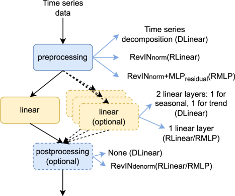
Figure 1: A common structure of linear-centric LTSF models.

4 Our Method: Mixture-of-Linear-Experts (MoLE)

We next introduce our proposed method: Mixture-of-Linear-Experts (MoLE). We use the shorthand MoLE-X (e.g., MoLE-DLinear) to refer to a linear-centric model X that has been augmented with MoLE.

4.1 Model Architecture

Our method, MoLE, acts as a plugin for existing and potential future linear-centric LTSF models. A typical linear LTSF model can be represented as shown in Figure 1. Figure 2 illustrates how our mixture-of-experts method integrates with an arbitrary linear-centric LTSF model. Initially, we group everything up to and including the linear layers into one head. Input time series data is passed to all heads, and the outputs from all heads are passed to the mixing layer (which acts as the router in mixture-of-experts). The mixing layer comprises a two-layered MLP, which accepts the embedding of the starting timestamp as input and produces one weight for the outputs of each head. These weights are channel-specific, meaning each channel will have distinct weight sets that sum to 1.

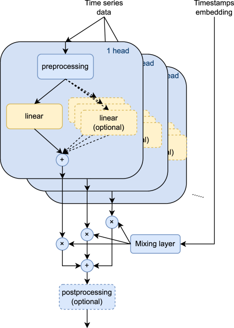
Figure 2: Structure of MoLE.

More precisely, this method can be described as follows: Let $\mathcal{H}_{i}$ represent the i-th head, where $\mathcal{H}_{i}:\mathbb{R}^{c\times s}\rightarrow\mathbb{R}^{c\times p}$, $c$ is the number of channels, $s$ is the input sequence length, and $p$ is the prediction length. Let $\mathcal{M}$ be the MLP layer in the mixing layer, where $\mathcal{M}:\mathbb{R}^{t}\rightarrow\mathbb{R}^{c\times n}$, $t$ being the length of the embedding of the first timestamp, and $n$ is the number of heads. Let $\mathcal{P}$ be the postprocessing layer, where $\mathcal{P}:\mathbb{R}^{c\times p}\rightarrow\mathbb{R}^{c\times p}$. If $\mathbf{X}\in\mathbb{R}^{c\times s}$ is the input time series data and $\mathbf{X}_{mark}\in\mathbb{R}^{t}$ is the embedding of the first element of the input time series, the output ($\mathbf{Z}$) of the entire system can be expressed as:

$$\mathbf{Y}_{i}=\mathcal{H}_{i}(\mathbf{X});~{}~{}\mathbf{W}=\mathcal{M}(\mathbf{X}_{mark})$$

$$\mathbf{Z}=\mathcal{P}(\sum_{i=1}^{n}\mathbf{W}_{:,i}\otimes\mathbf{Y}_{i})$$

Here, $\otimes$ is defined such that for a vector $\mathbf{a}\in\mathbb{R}^{c}$ and a matrix $\mathbf{B}\in\mathbb{R}^{c\times p}$, the operation $\mathbf{a}\otimes\mathbf{B}$ yields a new matrix $\mathbf{C}\in\mathbb{R}^{c\times p}$ where $C_{ij}=a_{i}\cdot B_{ij}$ for all $i$ and $j$.

Compared with the conventional Mixture of Experts (MoE) architecture where experts’ outputs are combined using a single weight, our proposed methodology (MoLE) introduces channel-wise awareness by having the mixing layer output a unique set of weights for each channel. In addition, instead of using the entire input data to determine gating, MoLE only uses the embedding of the first timestamp for gating. This reduces the overall number of parameters and exploits the structure of long-term time series, which typically exhibit (possibly non-stationary) time-dependence.

In our experiments, we use a simple linear normalization methods to embed datetime values, where various temporal components of a datetime value are encoded into uniformly spaced values between $[-0.5,0.5]$. We include the details of such embedding and the temporal components we chose for each dataset in Appendix A (Supplementary Material).

4.2 Toy Dataset

To show the intuitive effect of this approach, we first apply it to a toy dataset. We constructed the dataset such that from Monday to Thursday, the values adhere to a sinusoid function with frequency $f$. However, from Friday to Sunday, the values follow a sinusoid function with a doubled frequency of $2f$. Both have Gaussian noise added at each time step. This dataset exhibits weekly periodicity. The exact distribution is provided in B.1 in Supplementary Materials, and the first two weeks of the datasets are visualized in Figure 3.

[width=0.4]svg-inkscape/toy_dataset_svg-tex.pdf_tex

Figure 3: Visualization of the first 2 weeks (336 hours) of the toy dataset.

Experimental Setup

For this experiment, we use RLinear as the backbone. The setup includes an input sequence length of 24 (1 day), prediction length of 24 (1 day), batch size of 128, and an initial learning rate of 0.005. We restrict ourselves to only 2 heads for the MoLE-RLinear model in this experiment.

Results

Figure 4 demonstrates that the single-head RLinear model struggles to adapt to the pattern shift between Thursday and Friday. Even though the input sequence carries information (within timestamps 20-23) indicating the transition to Friday, the single-head RLinear model, due to its single-layer design, fails to make accurate predictions. In contrast, the 2-head MoLE-RLinear model captures this change well.

[width=0.5]svg-inkscape/toy_output_svg-tex.pdf_tex

Figure 4: Predictions of single-head RLinear model and multi(2)-head MoLE-RLinear model. The data from $t=0$ to $t=23$ is the input sequence, and the curves from $t=24$ onwards represent the ground truth and the predicted data from both methods.

5 Experiments

5.1 Experimental Setup

Datasets

Following the standard practice of prior work (Wu et al., 2021; Zhou et al., 2021; Zeng et al., 2023; Li et al., 2023), we conducted experiments on seven real-world datasets: the Electricity Transformer Temperature (ETT) datasets (ETTh1, ETTh2, ETTm1, ETTm2), as well as weather forecasting (Weather) (Angryk et al., 2020), electricity forecasting (Electricity) (Khan et al., 2020), and traffic flow estimation (Traffic) (Chen et al., 2001). We also include a very recent time series dataset, Weather2K (Zhu et al., 2023), which encompasses nearly three years of weather data from 1865 locations across China, featuring various weather conditions. We randomly selected four of these locations for evaluation: 79, 114, 850, 1786, which correspond to cities in the northeast, northwest, southwest, and south of China, respectively.

Table 1 provides a brief overview of these datasets. For the ETT datasets, data is split into training, validation, and test sets in a temporal order with a ratio of 6:2:2. For all other datasets, the split ratio is 7:1:2. The split ratios we have employed in our experiments are consistent with the methodologies used in prior work.

Table 1: Overview of Datasets

	Size	Granu-
Dataset	(Timestamps	larity
	$\times$Channels)
ETTh1,h2	17420 (725.83 days) $\times$ 7	1 hour
ETTm1,m2	69680 (725.83 days) $\times$ 7	15 minutes
Weather	52696 (365.86 days) $\times$ 21	10 minutes
Electricity	26304 (1096 days) $\times$ 321	1 hour
Traffic	17544 (731 days) $\times$ 336	1 hour
Weather2K	40896 (1704 days) $\times$ 20	1 hour

Baseline Models

We applied MoLE to three recent linear-centric LTSF models: DLinear (Zeng et al., 2023), RLinear (Li et al., 2023), and RMLP (Li et al., 2023). We refer to the original models as original and the models enhanced by our method as MoLE. Additionally, we evaluated the state-of-the-art transformer model, PatchTST (Nie et al., 2022). We assessed all models across every dataset, reproducing prior results of linear-centric models ourselves. Since PatchTST involved extensive hyperparameter search, we decided to use the author-reported results. Since PatchTST was not evaluated in the original paper on the newly released Weather2K dataset, we do not report PatchTST’s results for Weather2K. In our comparisons, we used the results of supervised PatchTST/64 and PatchTST/42. PatchTST/64 means the number of input patches is 64, which uses the look-back window $L=512$. PatchTST/42 means the number of input patches is 42, which has the default look-back window $L=336$. Our results on linear-centric models were mostly similar to reported results, so we use our computed values for our evaluation. In Appendix C (Supplementary Material), we give a complete table that compares the reported results from prior work to the values we obtained experimentally, and provide additional discussion of these variations. Additionally, we include the outcomes of further hyperparameter tuning to assess their impact on model performance in Appendix C.3.

Evaluation Metric

As in existing studies, we adopt the widely-used evaluation metric, mean squared error (MSE), which has been utilized in the works of Wu et al. (2021), Zhou et al. (2021), Zhang and Yan (2022), Zeng et al. (2023), and Li et al. (2023). The metric is defined as:

$$\operatorname{MSE}=\frac{1}{N}\sum_{i=1}^{N}(\mathbf{Y}_{i}-\hat{\mathbf{Y}}_{i})^{2}$$

where $N$ represents the total number of samples, $\mathbf{Y}_{i}$ indicates the i-th prediction, and $\hat{\mathbf{Y}}_{i}$ is the corresponding observation (ground truth).

Hyperparameters

For all our experiments, including ablations, we employed a grid search approach to determine the optimal hyperparameters for each setting, as detailed in Table 2. For every experiment, we utilized the set of hyperparameters that produced the lowest validation loss to report the test loss.

Sequence and prediction length. As in prior work Zeng et al. (2023); Li et al. (2023), we fix the input sequence length to 336. We vary the prediction length, or the number of time stamps for which we predict data, in the set $\{96,192,336,720\}$. We study the effect of variable input sequence length in Section 5.3.

Table 2: Hyperparameter search values.

Hyperparameter	Values
Batch size	8
Initial learning rate	0.005, 0.01, 0.05
Number of heads	2, 3, 4, 5, 6
Head dropout rate	0, 0.2
Input sequence length	336
Prediction length	{96,192,336,720}

Batch size. To narrow down our grid search, we conducted experiments to study how batch size influences model performance (Section 5.3). Based on our findings, we use a batch size of 8 for all experiments.

Initial learning rate. The choice of initial learning rate also impacts model performance. For our experiments, we selected three rates: 0.005, 0.01, and 0.05.

Number of heads. The number of heads in MoLE requires tuning to cater to the distinct characteristics of datasets. We swept between 2-6 heads.

Head dropout. To combat overfitting, we incorporated head dropout into MoLE. Throughout training, the weights originating from the mixing layer are randomly dropped at a rate of $r$. The retained weights are adjusted to ensure their combined sum is 1. We tested two rates: 0 (head dropout deactivated) and 0.2. We also provide a detailed analysis and comprehensive results on how the choice of dropout rate impacts multi-head model performance in Appendix D.2.

Implementation Details

For the conducted experiments, the mixing layer comprises a 2-layer MLP. The hidden layer dimension matches that of the output layer. A ReLU activation lies between the layers.

5.2 Comparison with Single-Head Models

Table 3: Comparison between original (single-head) and enhanced (multi-head MoLE) DLinear, RLinear, and RMLP models. Prediction length $\in\{96,192,336,720\}$. The values reported are MSE loss. A lower value indicates a better prediction. The better results among a linear-centric method and its MoLE variant is highlighted in bold. The cells shown in blue indicate the current SOTA for a given dataset and prediction length. For all three linear-centric models, MoLE improves forecasting error in over 78% of the datasets and settings we evaluated. Blank entries indicate datasets and prediction lengths that were not reported by the authors of PatchTST.

Model DLinear RLinear RMLP Dataset    Prediction length original MoLE original MoLE original MoLE ETTh1 96 0.372 0.377 0.371 0.375 0.381 0.421 192 0.413 0.453 0.404 0.403 0.541 0.432 336 0.442 0.469 0.428 0.430 0.453 0.437 720 0.501 0.505 0.450 0.449 0.502 0.474 ETTh2 96 0.287 0.287 0.272 0.273 0.294 0.322 192 0.349 0.362 0.341 0.336 0.362 0.375 336 0.430 0.419 0.372 0.371 0.389 0.416 720 0.710 0.605 0.418 0.409 0.440 0.418 ETTm1 96 0.300 0.286 0.301 0.291 0.300 0.294 192 0.336 0.328 0.335 0.333 0.339 0.340 336 0.374 0.380 0.371 0.368 0.365 0.365 720 0.461 0.447 0.429 0.429 0.439 0.426 ETTm2 96 0.168 0.168 0.164 0.163 0.165 0.163 192 0.228 0.233 0.219 0.217 0.223 0.220 336 0.295 0.289 0.272 0.272 0.282 0.282 720 0.382 0.399 0.368 0.380 0.362 0.371 weather 96 0.175 0.147 0.174 0.152 0.156 0.153 192 0.224 0.203 0.217 0.190 0.203 0.190 336 0.263 0.238 0.264 0.245 0.254 0.242 720 0.332 0.314 0.331 0.316 0.331 0.323 electricity 96 0.140 0.131 0.143 0.133 0.131 0.129 192 0.153 0.147 0.157 0.150 0.149 0.152 336 0.169 0.162 0.174 0.164 0.167 0.166 720 0.203 0.180 0.212 0.182 0.200 0.178 traffic 96 0.410 0.390 0.412 0.384 0.380 0.372 192 0.423 0.397 0.424 0.397 0.396 0.385 336 0.436 0.425 0.437 0.415 0.409 0.407 720 0.466 0.446 0.466 0.440 0.441 0.429 Weather2K79 96 0.571 0.555 0.572 0.564 0.584 0.567 192 0.593 0.566 0.595 0.588 0.601 0.588 336 0.590 0.546 0.592 0.575 0.594 0.574 720 0.619 0.535 0.624 0.566 0.616 0.565 Weather2K114 96 0.409 0.391 0.407 0.395 0.403 0.403 192 0.437 0.405 0.436 0.427 0.438 0.424 336 0.460 0.415 0.459 0.439 0.453 0.441 720 0.506 0.425 0.509 0.482 0.495 0.476 Weather2K850 96 0.481 0.474 0.483 0.471 0.481 0.483 192 0.502 0.484 0.505 0.495 0.509 0.495 336 0.509 0.474 0.513 0.502 0.513 0.499 720 0.523 0.461 0.527 0.489 0.527 0.491 Weather2K1786 96 0.545 0.535 0.545 0.535 0.550 0.544 192 0.591 0.601 0.591 0.581 0.600 0.584 336 0.620 0.603 0.620 0.618 0.634 0.617 720 0.658 0.660 0.660 0.628 0.668 0.640 No. improved (%) 32 (72.7%) 38 (86.4%) 33 (75.0%) PatchTST 64 42 0.370 0.375 0.413 0.414 0.422 0.431 0.447 0.449 0.274 0.274 0.341 0.339 0.329 0.331 0.379 0.379 0.293 0.290 0.333 0.332 0.369 0.366 0.416 0.420 0.166 0.165 0.223 0.220 0.274 0.278 0.362 0.367 0.149 0.152 0.194 0.197 0.245 0.249 0.314 0.320 0.129 0.130 0.147 0.148 0.163 0.167 0.197 0.202 0.360 0.367 0.379 0.385 0.392 0.398 0.432 0.434

Table 3 presents the evaluation results for three leading linear-centric models: DLinear, RLinear, and RMLP, across various datasets and prediction length settings. Among the 44 dataset and prediction length combinations, MoLE improves the forecasting error of the original model in 32/44 (73% of experiments) instances for DLinear, 38/44 (86%) instances for RLinear, and 33/44 (75% of experiments) instances for RMLP. In particular, we note that for larger datasets, such as weather, electricity, and traffic, MoLE enhances all 12 (100%) combinations of dataset and prediction length for DLinear and RLinear. The cells shown in blue indicate the current SOTA for a given dataset and prediction length. Enhanced by MoLE, these linear-centric models achieve SOTA in 68% of experimental settings for which PatchTST also reports numbers (to which we also compare), whereas the existing linear-centric models were previously SOTA in only 25% of cases. For the Weather2K datasets, MoLE-linear-centric models achieve SOTA in all settings.

5.3 Ablations and Design Choices

Does the timestamp input help the mixing layer learn better?

To demonstrate that the performance enhancement from MoLE is not just a result of increased model size, but rather the introduction of timestamp information, we designed the following experiments: 1) We replaced the timestamp embedding with random numbers (while keeping the values within the original range of the timestamp embedding). We call this variant RandomIn. 2) Building on the first ablation, we introduced a second modification where we use random weights instead of the outputs from the mixing layer to compute a weighted sum of the outputs from the heads. This is done both at training and test time. We call this variant RandomOut. We refer to the original MoLE with time stamp input as TimeIn. For these design variants, we maintained the same hyperparameter search strategy shown in Table 2. Consistent with our previous experiments, we chose the set of hyperparameters that produced the best validation loss to compute the reported test loss. We ran experiments using the DLinear model.

Table 4: Comparison between TimeIn (proposed method, conditioning on timestamp) with conditioning on a random input RandomIn and randomly mixing outputs RandomOut. The best MSE results are highlighted in bold, 2nd lowest losses are underlined. W2K stands for Weather2K datasets.

Data    Pred. Len. TimeIn RandomIn RandomOut ETTh1 96 0.3768 0.3750 0.3755 192 0.4531 0.4526 0.4297 336 0.4689 0.4742 0.4740 720 0.5046 0.5302 0.5229 ETTh2 96 0.2865 0.2916 0.2859 192 0.3617 0.3481 0.3618 336 0.4187 0.3864 0.4156 720 0.6053 0.5929 0.6029 ETTm1 96 0.2862 0.2865 0.3031 192 0.3281 0.3288 0.3357 336 0.3797 0.3712 0.3750 720 0.4466 0.4463 0.4506 ETTm2 96 0.1677 0.1678 0.1666 192 0.2334 0.2308 0.2252 336 0.2889 0.2828 0.2776 720 0.3985 0.4128 0.3807 Weather 96 0.1466 0.1454 0.1768 192 0.2025 0.1872 0.2240 336 0.2381 0.2461 0.2658 720 0.3142 0.3249 0.3335 Electricity 96 0.1314 0.1332 0.1399 192 0.1474 0.1472 0.1532 336 0.1618 0.1625 0.1688 720 0.1796 0.1974 0.2031 Traffic 96 0.3903 0.4096 0.4100 192 0.3966 0.4221 0.4226 336 0.4251 0.4338 0.4354 720 0.4460 0.4631 0.4655 W2K79 96 0.5547 0.5565 0.5711 192 0.5662 0.5810 0.5927 336 0.5465 0.5779 0.5900 720 0.5348 0.6012 0.6198 W2K114 96 0.3913 0.3894 0.4087 192 0.4053 0.4204 0.4371 336 0.4148 0.4424 0.4601 720 0.4246 0.4907 0.5066 W2K850 96 0.4741 0.4648 0.4804 192 0.4841 0.4931 0.5017 336 0.4745 0.5018 0.5091 720 0.4613 0.5089 0.5234 W2K1786 96 0.5346 0.5564 0.5459 192 0.6014 0.6025 0.5900 336 0.6034 0.6345 0.6177 720 0.6603 0.6827 0.6583 No. lowest 25/44 11/44 8/44

Surprisingly, RandomIn and RandomOut occasionally produce losses lower than TimeIn, which uses timestamp embeddings. This is consistent with the of findings of Roller et al. (2021) on MoE with hash layers. We explore why in the next subsection. For now, we comment on the robustness of TimeIn. As shown in Table 4, across all experiments, TimeIn had the lowest loss in 25 instances, surpassing RandomIn and RandomOut, which achieved this 11 and 8 times, respectively.

When, and why does randomness help?

We next try to understand when and why random inputs (and even outputs!) can help linear-centric models. We propose two possible effects contributing to this observation: Effect 1: RandomIn and RandomOut may have a regularization effect, akin to dropout (Baldi and Sadowski, 2013), which prevents the network from overfitting head weights to the training data. This has the effect of making all heads better. Effect 2: Suppose time series can be roughly divided into regimes with different temporal patterns (e.g., weekdays vs weekends). For long input sequences, the sequence may traverse multiple regimes. Hence, no single head will be able to capture the full dynamics, regardless of start time. However, as the input sequence lengthens, the linear layer has more past data to consider, and some patterns in this data can hint at upcoming changes in the series. Hence, we predict that the effect of conditioning on start time should be less beneficial. Conversely, as the input sequence length is reduced, the effect of input time should be more beneficial.

We hypothesize that both effects contribute to the observations in Table 4. To validate this hypothesis, we conducted the following experiment on MoLE-DLinear. To test effect 1, we compared TimeIn, RandomIn, and RandomOut to a variant in which we conduct dropout over the heads. That is, during training, we exclude in each iteration a randomly-selected fraction (20%) of heads. At test time, we use all heads according to the learned weights in the mixing layer. To test effect 2, we fixed the prediction length to 100 and progressively varied the input sequence length among $\{6,88,170,254,336\}$.

Following the same methodology as our main experiments, we performed a grid search on hyperparameters and reported the test loss of the best set of hyperparameters for each seed. Each experiment is averaged over three runs over the Electricity dataset.

In Figure 5, we plot the mean MSE for each input length, and the shadows around the curves represent the $\pm$ standard deviation. The shadows are not clearly visible since the results are stable. Figure 5 illustrates three important trends:

(1) As input length increases, the performance of TimeIn approaches that of the single-head baseline, as well as RandomIn and RandomOut. This suggests that Effect 2 may indeed be correct: conditioning on timestamp is more beneficial as input sequence length decreases. (Note that our earlier results in Table 3 used a fixed input length of 336, which is the rightmost point of Figure 5, where the gains of MoLE are least pronounced.)

[width=0.5]svg-inkscape/ecl_small_input_svg-tex.pdf_tex

Figure 5: Performance comparison of various methods based on input length on MoLE-DLinear.

[width=0.5]svg-inkscape/batch_size_svg-tex.pdf_tex

Figure 6: Impact of batch size on MoLE-DLinear

(2) Dropout has virtually no effect on RandomIn or RandomOut, but it does affect TimeIn. This suggests that using random inputs may indeed have a regularization effect (Effect 1), which is roughly equivalent to dropout over heads. To take advantage of both effects at once, we can condition on time stamp while also doing dropout over heads.

(3) As input sequence length grows, the effect of dropout on TimeIn becomes more beneficial. This suggests that overfitting to the start timestamp is more detrimental for longer input sequences.

How does batch size influence model performance and what size should we use?

We finally present the results of our experiments to determine the batch size for our prior experiments. Figure 6 plots how the final test loss varies with batch size, for four datasets. For these experiments, we used DLinear as the base model, with an input sequence length of 336, prediction length of 96, five heads, and an initial learning rate of 0.05. We observe that in general, test losses are lower when batch sizes are either very small or (in some cases) large (relative to intermediate sizes ranging from 16 to 128). This mid-range of batch sizes exhibits poor generalization, with low training loss but high test loss, similar to observations in Keskar et al. (2016). For robustness, we used a batch size of 8. Comprehensive results and a more detailed analysis of batch size effects are available in the Appendix D.1.

6 Conclusion and Future Work

We propose MoLE, a technique based on mixture-of-experts that can be applied out-of-the-box to existing linear-centric models to improve performance in the LTSF problem. Our results strongly suggest that MoLE gives significant and robust gains across a wide range of datasets and prediction settings. An important open question is precisely characterizing high-dimensional datasets to understand exactly when MoLE will help. Although we hypothesize that this question relates to the degree and patterns of nonstationarity in the time series dataset, it is currently unclear how to predict how many heads are needed.

Appendix A Time Stamp Embedding

In the preprocessing of date-time information for our datasets, various time-based features are extracted from the timestamp data. Each feature corresponds to a specific component of the timestamp, including the hour of the day, day of the week, day of the month, and day of the year. These features are each encoded into a range of $-0.5$ to $0.5$, with the transformation depending on the possible range of each feature.

For instance, in the case of the day of the week, Monday is indexed as $0$ and Sunday as $6$. Each day of the week is then encoded to a value between $-0.5$ and $0.5$, with the transformation given by the formula

$$\left(\frac{\text{index}}{6}\right)-0.5$$

Thus, Monday would be encoded as $-0.5$, Tuesday as approximately $-0.33$, Wednesday as approximately $-0.17$, and so on, with Sunday encoded as $0.5$.

Appendix B Toy Dataset Experiments

B.1 Dataset Description

We construct a toy dataset that models periodic behaviors across different days of the week. Precisely, the dataset can be written as:

$$y(t)=\begin{cases}y_{M-T}(t)+\text{noise}(t)&\text{Monday to Thursday}\\ y_{F-S}(t)+\text{noise}(t)&\text{Friday to Sunday}\end{cases}$$

where

$$y_{M-T}(t)=6\sin\left(2\pi\frac{1}{24}t\right)+20$$

$$y_{F-S}(t)=6\sin\left(2\pi\frac{1}{12}t\right)+20$$

$$\text{noise}(t)\sim\mathcal{N}(0,0.1^{2})$$

B.2 More detailed results from the toy dataset experiments

[width=]svg-inkscape/mixing_weight_svg-tex.pdf_tex

((a)) How mixing weights change with time

[width=]svg-inkscape/single-head_weight_svg-tex.pdf_tex

((b)) Weights of the linear layer in single-head model

[width=]svg-inkscape/multi-head_weight-1_svg-tex.pdf_tex

((c)) Weights of the linear layer in the 1st head of multi-head model

[width=]svg-inkscape/multi-head_weight-2_svg-tex.pdf_tex

((d)) Weights of the linear layer in the 2nd head of multi-head model

Figure 7: More detailed look into the experiment of the toy examples. In heatmaps, a bright color indicates a positive value while a dark color indicates a negative value.

Figure 7(a) shows how the mixing weights change over a continuous 2-week period. The mixing layer captures the temporal patterns in the data, applying different heads for different frequencies. Figure 7(b) is a heatmap representing the weight distribution of the linear layer in the single-head model. Using one head to predict the time series, the model derives a compromised weight set that underperforms, as shown in Figure 4. However, when employing two heads, the resulting models—whose linear layer weights are depicted in Figures 7(c) and 7(d)—efficiently learn the two frequency patterns and can yield more accurate predictions.

Appendix C Additional Main Results

C.1 Comparing Original and Our Replicated Experiments.

In this section, we compare previously-reported results with our reproduction of prior linear-centric results (using their code).

Table 5 illustrates the differences between the original findings (Auth.) and our replicated experiments (Reprod.). On average, the DLinear model’s outcomes vary by roughly 1.04% from the original. Meanwhile, the RMLP and RLinear models show variations of around 2.10% and 1.99% respectively, indicating a generally consistent replication.

Table 5: Comparison of author’s original results (Auth.) with reproduced results (Reprod.) Prediction length $\in\{96,192,336,720\}$. The values reported are MSE loss. A lower value indicates a better prediction. The Difference (Diff.) represents the relative differences from the original results, computed as $\text{Diff.}=(\text{Reprod.}-\text{Auth.})/{\text{Auth.}}\times 100\%$. Blank entries indicate datasets and prediction lengths that were not reported by the authors.

Model
ETTh1	96
	192
	336
	720
ETTh2	96
	192
	336
	720
ETTm1	96
	192
	336
	720
ETTm2	96
	192
	336
	720
weather	96
	192
	336
	720
electricity	96
	192
	336
	720
traffic	96
	192
	336
	720
Avg. Diff.

DLinear			RLinear			RMLP
Auth.	Reprod.	Diff.	Auth.	Reprod.	Diff.	Auth.	Reprod.	Diff.
0.375	0.372	-0.80%	0.366	0.371	1.37%	0.390	0.381	-2.31%
0.405	0.413	1.98%	0.404	0.404	0.00%	0.430	0.541	25.81%
0.439	0.442	0.68%	0.420	0.428	1.90%	0.441	0.453	2.72%
0.472	0.501	6.14%	0.442	0.45	1.81%	0.506	0.502	-0.79%
0.289	0.287	-0.69%	0.262	0.272	3.82%	0.288	0.294	2.08%
0.383	0.349	-8.88%	0.319	0.341	6.90%	0.343	0.362	5.54%
0.448	0.430	-4.02%	0.325	0.372	14.46%	0.353	0.389	10.20%
0.605	0.710	17.36%	0.372	0.418	12.37%	0.410	0.440	7.32%
0.299	0.300	0.33%	0.301	0.301	0.00%	0.298	0.300	0.67%
0.335	0.336	0.30%	0.335	0.335	0.00%	0.344	0.339	-1.45%
0.369	0.374	1.36%	0.370	0.371	0.27%	0.390	0.365	-6.41%
0.425	0.461	8.47%	0.425	0.429	0.94%	0.445	0.439	-1.35%
0.167	0.168	0.60%	0.164	0.164	0.00%	0.174	0.165	-5.17%
0.224	0.228	1.79%	0.219	0.219	0.00%	0.236	0.223	-5.51%
0.281	0.295	4.98%	0.273	0.272	-0.37%	0.291	0.282	-3.09%
0.397	0.382	-3.78%	0.366	0.368	0.55%	0.371	0.362	-2.43%
0.176	0.175	-0.57%	0.175	0.174	-0.57%	0.149	0.156	4.70%
0.220	0.224	1.82%	0.218	0.217	-0.46%	0.194	0.203	4.64%
0.265	0.263	-0.75%	0.265	0.264	-0.38%	0.243	0.254	4.53%
0.323	0.332	2.79%	0.329	0.331	0.61%	0.316	0.331	4.75%
0.140	0.140	0.00%	0.140	0.143	2.14%	0.129	0.131	1.55%
0.153	0.153	0.00%	0.154	0.157	1.95%	0.147	0.149	1.36%
0.169	0.169	0.00%	0.171	0.174	1.75%	0.164	0.167	1.83%
0.203	0.203	0.00%	0.209	0.212	1.44%	0.203	0.200	-1.48%
0.410	0.410	0.00%		0.412			0.380
0.423	0.423	0.00%		0.424			0.396
0.436	0.436	0.00%		0.437			0.409
0.466	0.466	0.00%		0.446			0.441
		1.04%			2.10%			1.99%

C.2 Results with Different Random Seeds

Additionally, we conducted robustness experiments on all datasets except for Weather2K. Instead of utilizing a single seed (2021), we employed three different seeds (2021, 2022, 2023) and calculated the average losses from these runs. Within each run, the reported losses still adhere to our primary experimental method where we chose the test losses of hyperparameters that resulted in the lowest validation losses.

Table 6 presents the results of our robustness tests. Here, MoLE exhibited improvements over the DLinear model in 16 settings, and over RLinear and RMLP in 21 and 19 settings, respectively. The average enhancements exceed 67.7%. This demonstrates that our methodology remains consistent across varied random seeds and consistently enhances the performance of the linear-centric models we tested.

Table 6: Comparison between original (single-head) and enhanced (multi-head MoLE) DLinear, RLinear, and RMLP models. Each experiment is conducted using three different random seeds: 2021, 2022, 2023. The average losses (avg) and standard deviations (stdev) are reported. Prediction length $\in\{96,192,336,720\}$. The values reported are MSE loss. A lower value indicates a better prediction. The cells shown in blue indicate that MoLE improves the performance of the original (single-head) models.

Model
ETTh1	96
	192
	336
	720
ETTh2	96
	192
	336
	720
ETTm1	96
	192
	336
	720
ETTm2	96
	192
	336
	720
weather	96
	192
	336
	720
electricity	96
	192
	336
	720
traffic	96
	192
	336
	720
IMP

DLinear				RLinear				RMLP
original		MoLE		original		MoLE		original		MoLE
avg	stdev	avg	stdev	avg	stdev	avg	stdev	avg	stdev	avg	stdev
0.3741	2.29e-3	0.3824	1.58e-2	0.3711	1.67e-3	0.3742	2.12e-3	0.3833	2.20e-3	0.4109	7.29e-3
0.4134	7.83e-3	0.4291	2.53e-2	0.4052	1.60e-3	0.4105	6.61e-3	0.4914	4.75e-2	0.4403	1.06e-2
0.4499	1.14e-2	0.4557	2.16e-3	0.4291	1.52e-3	0.5252	1.67e-1	0.5028	2.86e-2	0.4433	8.53e-3
0.5072	1.76e-2	0.5136	3.02e-2	0.4483	4.01e-4	0.4493	2.18e-4	0.5072	1.54e-2	0.4830	1.19e-2
0.2824	4.96e-3	0.2842	3.68e-3	0.2730	2.02e-3	0.2737	6.71e-4	0.2943	4.31e-4	0.2979	7.74e-3
0.3566	6.84e-3	0.3652	2.32e-2	0.3471	5.95e-3	0.3401	2.40e-3	0.3683	9.96e-3	0.4028	7.25e-2
0.4162	2.48e-2	0.4191	2.62e-3	0.3754	3.47e-3	0.3770	7.80e-3	0.3926	1.24e-2	0.4044	1.02e-2
0.6648	5.46e-2	0.6238	8.74e-2	0.4233	3.55e-3	0.3918	6.08e-3	0.4444	1.61e-2	0.4206	9.33e-3
0.2998	3.31e-4	0.2879	1.14e-3	0.3024	1.73e-3	0.2925	4.47e-3	0.2968	3.58e-3	0.2983	1.86e-3
0.3358	2.84e-4	0.3349	7.72e-3	0.3402	3.79e-3	0.3313	2.12e-3	0.3365	3.25e-3	0.3348	3.32e-3
0.3794	5.20e-3	0.3731	4.19e-3	0.3714	8.36e-4	0.3692	1.82e-3	0.3729	3.30e-3	0.3697	5.22e-3
0.4400	1.13e-3	0.4486	1.82e-2	0.4274	2.05e-3	0.4271	9.96e-4	0.4306	2.64e-3	0.4284	3.20e-3
0.1680	9.57e-4	0.1684	2.80e-3	0.1636	9.65e-4	0.1622	6.40e-4	0.1672	3.59e-3	0.1672	4.86e-3
0.2291	7.67e-4	0.2286	3.18e-3	0.2195	7.68e-4	0.2170	3.70e-4	0.2216	2.35e-3	0.2190	1.20e-3
0.2875	9.00e-3	0.2956	5.78e-3	0.2724	3.48e-4	0.2720	7.32e-4	0.2807	5.57e-3	0.2792	4.38e-3
0.3990	1.73e-2	0.4082	1.29e-3	0.3678	3.03e-4	0.3688	2.16e-3	0.3680	4.33e-3	0.3729	6.62e-3
0.1748	2.05e-4	0.1599	2.33e-2	0.1742	6.24e-5	0.1506	4.39e-3	0.1560	1.99e-3	0.1549	9.27e-3
0.2182	4.63e-3	0.2014	9.50e-3	0.2166	6.24e-4	0.1890	7.38e-4	0.2037	1.67e-3	0.1952	5.40e-3
0.2656	5.52e-3	0.3201	1.33e-1	0.2640	2.34e-4	0.2449	5.00e-3	0.2564	2.49e-3	0.2464	1.79e-3
0.3295	3.03e-3	0.3125	1.93e-3	0.3311	6.52e-5	0.3204	5.97e-3	0.3269	2.52e-3	0.3931	1.06e-1
0.1399	4.70e-6	0.1289	3.64e-4	0.1432	2.74e-5	0.1319	1.72e-4	0.1307	6.23e-4	0.1290	6.40e-4
0.1533	1.75e-6	0.1475	2.90e-4	0.1568	1.79e-6	0.1513	4.82e-4	0.1497	2.62e-4	0.1511	1.73e-3
0.1689	6.38e-6	0.1611	1.26e-3	0.1735	5.27e-6	0.1647	1.04e-3	0.1660	6.25e-4	0.1657	2.61e-3
0.2032	6.36e-5	0.1787	1.06e-3	0.2122	6.06e-5	0.1842	4.38e-3	0.2022	1.11e-3	0.1795	9.70e-4
0.4102	2.60e-5	0.3843	1.25e-3	0.4119	6.46e-6	0.3783	2.29e-3	0.3786	2.70e-3	0.3695	3.48e-3
0.4226	3.88e-5	0.3957	4.27e-3	0.4243	2.42e-5	0.3949	3.21e-3	0.3967	5.31e-4	0.3852	2.46e-3
0.4355	3.40e-5	0.4239	3.08e-3	0.4367	2.14e-5	0.4158	2.31e-3	0.4092	1.13e-4	0.4080	5.02e-3
0.4657	8.93e-5	0.4533	4.88e-3	0.4655	4.47e-6	0.4538	2.25e-3	0.4436	1.59e-3	0.4408	1.27e-3
16 (57.1%)				21 (75.0%)				19 (67.9%)

C.3 Results with Additional Hyperparameter Tuning

We are interested in understanding the comprehensive impact of batch sizes and head dropout rates on model performance. To explore this, we have added additional values of these hyperparameters into our hyperparameter tuning process. Due to the high costs of these experiments and their similar performance compared to the hyperparameter tuning shown in our main text, their results are presented only here in the Appendix. The grid search included the following sets of hyperparameters in Table 7.

Table 7: Hyperparameter search values. Bold denotes newly added hyperparameter values.

Hyperparameter	Values
Batch size	8, 16, 32, 64, 128
Initial learning rate	0.005, 0.01, 0.05
Number of heads	2, 3, 4, 5, 6
Head dropout rate	0, 0.2, 0.4, 0.6, 0.8
Input sequence length	336
Prediction length	{96,192,336,720}

Our methodology mirrors that of our primary experiments, where test losses correspond to hyperparameters yielding the lowest validation losses. Moreover, each experiment was conducted three times using distinct random seeds (2021, 2022, and 2023). The best results from each seed were averaged to obtain the final reported outcomes. The results in Table 8 show that adding new hyperparameter values did not improve model performance. This suggests that the original set of hyperparameters was sufficient for representing each model’s capabilities.

Table 8: Comparison between original (single-head) and enhanced (multi-head MoLE) DLinear, RLinear, and RMLP models with added hyperparameter values. Prediction length $\in\{96,192,336,720\}$. The values reported are MSE loss. A lower value indicates a better prediction. The better results among a linear-centric method and its MoLE variant is highlighted in bold.

Model		DLinear		RLinear		RMLP
Dataset    Prediction length		original	MoLE	original	MoLE	original	MoLE
ETTh1	96	0.376	0.375	0.370	0.374	0.387	0.381
	192	0.411	0.436	0.405	0.408	0.434	0.425
	336	0.456	0.474	0.427	0.433	0.462	0.437
	720	0.498	0.497	0.447	0.446	0.514	0.524
ETTh2	96	0.282	0.282	0.275	0.275	0.304	0.285
	192	0.362	0.359	0.349	0.349	0.371	0.372
	336	0.403	0.403	0.378	0.361	0.399	0.398
	720	0.610	1.378	0.423	0.389	0.448	0.418
ETTm1	96	0.301	0.295	0.304	0.290	0.302	0.296
	192	0.344	0.347	0.341	0.339	0.341	0.334
	336	0.382	0.384	0.374	0.372	0.373	0.374
	720	0.451	0.466	0.428	0.429	0.432	0.428
ETTm2	96	0.166	0.165	0.164	0.162	0.170	0.169
	192	0.228	0.223	0.220	0.220	0.222	0.228
	336	0.279	0.276	0.273	0.272	0.281	0.273
	720	0.392	0.386	0.367	0.370	0.369	0.371
weather	96	0.176	0.160	0.174	0.149	0.152	0.152
	192	0.217	0.210	0.217	0.195	0.194	0.194
	336	0.266	0.300	0.265	0.243	0.244	0.246
	720	0.334	0.332	0.331	0.316	0.325	0.322
electricity	96	0.140	0.130	0.143	0.132	0.130	0.128
	192	0.153	0.147	0.154	0.149	0.148	0.149
	336	0.169	0.160	0.172	0.164	0.164	0.163
	720	0.203	0.180	0.211	0.189	0.202	0.178
traffic	96	0.409	0.384	0.412	0.383	0.376	0.367
	192	0.420	0.400	0.423	0.399	0.396	0.385
	336	0.436	0.419	0.437	0.413	0.409	0.402
	720	0.466	0.448	0.465	0.444	0.443	0.435
No. improved (%)		19 (67.9%)		20 (71.4%)		19 (67.9%)

Appendix D Additional Ablations

Based on the results of the full hyperparameter tuning shown in Appendix C.3, we conducted two additional ablations to further discuss how the choices of batch sizes and head dropout rates impact model performance. The plots that follow show curves which are the average test losses from three different seeds. These test losses are chosen from the hyperparameter configurations that yielded the lowest validation losses, while keeping the parameter on the x-axis constant. The shaded regions around each curve indicate the range of $\pm$ one standard deviation.

D.1 Impact of Batch Sizes on Model Performance

Figure 8 demonstrates the impact of varying batch sizes on the performance of both single-head and MoLE DLinear, RLinear, and RMLP models. For smaller datasets, such as the ETT series, there is a trend similar to an inverse U-shape, suggesting that very small or very large batch sizes may enhance model performance. In contrast, for larger datasets, particularly electricity and traffic, larger batch sizes appear to benefit single-head models, while MoLE models show optimal performance with mid-range to small batch sizes. Importantly, in large datasets, MoLE models consistently outperform single-head models, even when the latter are given the advantage of larger batch sizes. This trend is also observable in Table 8, where comprehensive hyperparameter tuning does not enable single-head models to outperform MoLE in large datasets. These results confirm that the batch size of 8, used in our main experiments, is sufficient to effectively represent each model’s capabilities.

[width=]svg-inkscape/batch_size_DLinear_svg-tex.pdf_tex

((a)) DLinear

[width=]svg-inkscape/batch_size_RLinear_svg-tex.pdf_tex

((b)) RLinear

[width=]svg-inkscape/batch_size_RMLP_svg-tex.pdf_tex

((c)) RMLP

Figure 8: Subplot comparison of test loss versus batch sizes across different prediction lengths and datasets. First row of each subplot: single-head (Original) models. Second row: MoLE models.

D.2 Impact of Head Dropout Rates on MoLE Performance

Figure 9 illustrates the test loss as a function of dropout rates for three distinct models: DLinear, RLinear, and RMLP, across various datasets.

For the DLinear model, there is a consistent trend across datasets where certain mid-range dropout rates yield lower test losses, such as in the ETTm1, weather, electricity, and traffic datasets. For RLinear and RMLP, similar U-shaped patterns can be observed, but only in larger datasets such as weather, electricity, and traffic. For smaller datasets, like the ETT series, the link between dropout rate and test loss isn’t clear. The plots show a lot of variation, indicating that the relationship is not strong.

[width=]svg-inkscape/dropout_rate_DLinear_svg-tex.pdf_tex

((a)) DLinear

[width=]svg-inkscape/dropout_rate_RLinear_svg-tex.pdf_tex

((b)) RLinear

[width=]svg-inkscape/dropout_rate_RMLP_svg-tex.pdf_tex

((c)) RMLP

Figure 9: Subplot comparison of test loss against head dropout rates for MoLE models across various prediction lengths and datasets.

Appendix E Anonymous Source Code

The code associated with this research can be accessed at https://anonymous.4open.science/r/MoLE.

References

- Angryk et al. (2020) Rafal A Angryk, Petrus C Martens, Berkay Aydin, Dustin Kempton, Sushant S Mahajan, Sunitha Basodi, Azim Ahmadzadeh, Xumin Cai, Soukaina Filali Boubrahimi, Shah Muhammad Hamdi, et al. Multivariate time series dataset for space weather data analytics. Scientific data, 7(1):227, 2020.
- Ariyo et al. (2014) Adebiyi A Ariyo, Adewumi O Adewumi, and Charles K Ayo. Stock price prediction using the arima model. In 2014 UKSim-AMSS 16th international conference on computer modelling and simulation, pages 106–112. IEEE, 2014.
- Artetxe et al. (2021) Mikel Artetxe, Shruti Bhosale, Naman Goyal, Todor Mihaylov, Myle Ott, Sam Shleifer, Xi Victoria Lin, Jingfei Du, Srinivasan Iyer, Ramakanth Pasunuru, et al. Efficient large scale language modeling with mixtures of experts. arXiv preprint arXiv:2112.10684, 2021.
- Bai et al. (2018) Shaojie Bai, J Zico Kolter, and Vladlen Koltun. An empirical evaluation of generic convolutional and recurrent networks for sequence modeling. arXiv preprint arXiv:1803.01271, 2018.
- Baldi and Sadowski (2013) Pierre Baldi and Peter J Sadowski. Understanding dropout. Advances in neural information processing systems, 26, 2013.
- Borovykh et al. (2017) Anastasia Borovykh, Sander Bohte, and Cornelis W Oosterlee. Conditional time series forecasting with convolutional neural networks. arXiv preprint arXiv:1703.04691, 2017.
- BOX (1976) G BOX. Time series analysis forecasting and control. Holden-Day, Oackland. California 1976, 1976.
- Chang et al. (2018) Yen-Yu Chang, Fan-Yun Sun, Yueh-Hua Wu, and Shou-De Lin. A memory-network based solution for multivariate time-series forecasting. arXiv preprint arXiv:1809.02105, 2018.
- Chen et al. (2001) Chao Chen, Karl Petty, Alexander Skabardonis, Pravin Varaiya, and Zhanfeng Jia. Freeway performance measurement system: mining loop detector data. Transportation Research Record, 1748(1):96–102, 2001.
- Chen et al. (2023) Si-An Chen, Chun-Liang Li, Nate Yoder, Sercan O Arik, and Tomas Pfister. Tsmixer: An all-mlp architecture for time series forecasting. arXiv preprint arXiv:2303.06053, 2023.
- Das et al. (2023) Abhimanyu Das, Weihao Kong, Andrew Leach, Rajat Sen, and Rose Yu. Long-term forecasting with tide: Time-series dense encoder. arXiv preprint arXiv:2304.08424, 2023.
- Dryden and Hoefler (2022) Nikoli Dryden and Torsten Hoefler. Spatial mixture-of-experts. Advances in Neural Information Processing Systems, 35:11697–11713, 2022.
- Du et al. (2023) Dazhao Du, Bing Su, and Zhewei Wei. Preformer: predictive transformer with multi-scale segment-wise correlations for long-term time series forecasting. In ICASSP 2023-2023 IEEE International Conference on Acoustics, Speech and Signal Processing (ICASSP), pages 1–5. IEEE, 2023.
- Fan et al. (2019) Chenyou Fan, Yuze Zhang, Yi Pan, Xiaoyue Li, Chi Zhang, Rong Yuan, Di Wu, Wensheng Wang, Jian Pei, and Heng Huang. Multi-horizon time series forecasting with temporal attention learning. In Proceedings of the 25th ACM SIGKDD International conference on knowledge discovery & data mining, pages 2527–2535, 2019.
- Fildes (1991) Robert Fildes. Forecasting, structural time series models and the kalman filter: Bayesian forecasting and dynamic models. Journal of the Operational Research Society, 42(11):1031–1033, 1991.
- Gong et al. (2023) Zeying Gong, Yujin Tang, and Junwei Liang. Patchmixer: A patch-mixing architecture for long-term time series forecasting. arXiv preprint arXiv:2310.00655, 2023.
- Gruver et al. (2023) Nate Gruver, Marc Finzi, Shikai Qiu, and Andrew Gordon Wilson. Large language models are zero-shot time series forecasters. arXiv preprint arXiv:2310.07820, 2023.
- Han et al. (2019) Zhongyang Han, Jun Zhao, Henry Leung, King Fai Ma, and Wei Wang. A review of deep learning models for time series prediction. IEEE Sensors Journal, 21(6):7833–7848, 2019.
- Jiang et al. (2023) Jiawei Jiang, Chengkai Han, Wayne Xin Zhao, and Jingyuan Wang. Pdformer: Propagation delay-aware dynamic long-range transformer for traffic flow prediction. In AAAI. AAAI Press, 2023.
- Jordan and Jacobs (1994) Michael I Jordan and Robert A Jacobs. Hierarchical mixtures of experts and the em algorithm. Neural computation, 6(2):181–214, 1994.
- Keskar et al. (2016) Nitish Shirish Keskar, Dheevatsa Mudigere, Jorge Nocedal, Mikhail Smelyanskiy, and Ping Tak Peter Tang. On large-batch training for deep learning: Generalization gap and sharp minima. arXiv preprint arXiv:1609.04836, 2016.
- Khan et al. (2020) Zulfiqar Ahmad Khan, Tanveer Hussain, Amin Ullah, Seungmin Rho, Miyoung Lee, and Sung Wook Baik. Towards efficient electricity forecasting in residential and commercial buildings: A novel hybrid cnn with a lstm-ae based framework. Sensors, 20(5):1399, 2020.
- Kim et al. (2021) Taesung Kim, Jinhee Kim, Yunwon Tae, Cheonbok Park, Jang-Ho Choi, and Jaegul Choo. Reversible instance normalization for accurate time-series forecasting against distribution shift. In International Conference on Learning Representations, 2021.
- Lai et al. (2018) Guokun Lai, Wei-Cheng Chang, Yiming Yang, and Hanxiao Liu. Modeling long-and short-term temporal patterns with deep neural networks. In The 41st international ACM SIGIR conference on research & development in information retrieval, pages 95–104, 2018.
- Li et al. (2023) Zhe Li, Shiyi Qi, Yiduo Li, and Zenglin Xu. Revisiting long-term time series forecasting: An investigation on linear mapping. arXiv preprint arXiv:2305.10721, 2023.
- Liu et al. (2021) Shizhan Liu, Hang Yu, Cong Liao, Jianguo Li, Weiyao Lin, Alex X Liu, and Schahram Dustdar. Pyraformer: Low-complexity pyramidal attention for long-range time series modeling and forecasting. In International conference on learning representations, 2021.
- Nie et al. (2022) Yuqi Nie, Nam H Nguyen, Phanwadee Sinthong, and Jayant Kalagnanam. A time series is worth 64 words: Long-term forecasting with transformers. arXiv preprint arXiv:2211.14730, 2022.
- Riquelme et al. (2021) Carlos Riquelme, Joan Puigcerver, Basil Mustafa, Maxim Neumann, Rodolphe Jenatton, André Susano Pinto, Daniel Keysers, and Neil Houlsby. Scaling vision with sparse mixture of experts. Advances in Neural Information Processing Systems, 34:8583–8595, 2021.
- Roller et al. (2021) Stephen Roller, Sainbayar Sukhbaatar, Jason Weston, et al. Hash layers for large sparse models. Advances in Neural Information Processing Systems, 34:17555–17566, 2021.
- Shao et al. (2022) Zezhi Shao, Zhao Zhang, Fei Wang, Wei Wei, and Yongjun Xu. Spatial-temporal identity: A simple yet effective baseline for multivariate time series forecasting. In Proceedings of the 31st ACM International Conference on Information & Knowledge Management, pages 4454–4458, 2022.
- Shazeer et al. (2017) Noam Shazeer, Azalia Mirhoseini, Krzysztof Maziarz, Andy Davis, Quoc Le, Geoffrey Hinton, and Jeff Dean. Outrageously large neural networks: The sparsely-gated mixture-of-experts layer. arXiv preprint arXiv:1701.06538, 2017.
- Shen et al. (2023) Sheng Shen, Le Hou, Yanqi Zhou, Nan Du, Shayne Longpre, Jason Wei, Hyung Won Chung, Barret Zoph, William Fedus, Xinyun Chen, et al. Flan-moe: Scaling instruction-finetuned language models with sparse mixture of experts. arXiv preprint arXiv:2305.14705, 2023.
- Wang et al. (2022) Huiqiang Wang, Jian Peng, Feihu Huang, Jince Wang, Junhui Chen, and Yifei Xiao. Micn: Multi-scale local and global context modeling for long-term series forecasting. In The Eleventh International Conference on Learning Representations, 2022.
- Wang et al. (2023a) Wei Wang, Yang Liu, and Hao Sun. Tlnets: Transformation learning networks for long-range time-series prediction. arXiv preprint arXiv:2305.15770, 2023a.
- Wang et al. (2023b) Zepu Wang, Yuqi Nie, Peng Sun, Nam H Nguyen, John Mulvey, and H Vincent Poor. St-mlp: A cascaded spatio-temporal linear framework with channel-independence strategy for traffic forecasting. arXiv preprint arXiv:2308.07496, 2023b.
- Wen et al. (2022) Qingsong Wen, Tian Zhou, Chaoli Zhang, Weiqi Chen, Ziqing Ma, Junchi Yan, and Liang Sun. Transformers in time series: A survey. arXiv preprint arXiv:2202.07125, 2022.
- Wu et al. (2021) Haixu Wu, Jiehui Xu, Jianmin Wang, and Mingsheng Long. Autoformer: Decomposition transformers with auto-correlation for long-term series forecasting. Advances in Neural Information Processing Systems, 34:22419–22430, 2021.
- Wu et al. (2023) Haixu Wu, Hang Zhou, Mingsheng Long, and Jianmin Wang. Interpretable weather forecasting for worldwide stations with a unified deep model. Nature Machine Intelligence, 5(6):602–611, June 2023. ISSN 2522-5839. doi: 10.1038/s42256-023-00667-9. URL https://doi.org/10.1038/s42256-023-00667-9.
- Xu et al. (2023) Zhijian Xu, Ailing Zeng, and Qiang Xu. Fits: Modeling time series with parameters. arXiv preprint arXiv:2307.03756, 2023.
- Yi et al. (2023) Rongjie Yi, Liwei Guo, Shiyun Wei, Ao Zhou, Shangguang Wang, and Mengwei Xu. Edgemoe: Fast on-device inference of moe-based large language models. arXiv preprint arXiv:2308.14352, 2023.
- Yuksel et al. (2012) Seniha Esen Yuksel, Joseph N. Wilson, and Paul D. Gader. Twenty years of mixture of experts. IEEE Transactions on Neural Networks and Learning Systems, 23(8):1177–1193, 2012. doi: 10.1109/TNNLS.2012.2200299.
- Zeng et al. (2023) Ailing Zeng, Muxi Chen, Lei Zhang, and Qiang Xu. Are transformers effective for time series forecasting? In Proceedings of the AAAI conference on artificial intelligence, volume 37, pages 11121–11128, 2023.
- Zhang et al. (2022) Tianping Zhang, Yizhuo Zhang, Wei Cao, Jiang Bian, Xiaohan Yi, Shun Zheng, and Jian Li. Less is more: Fast multivariate time series forecasting with light sampling-oriented mlp structures. arXiv preprint arXiv:2207.01186, 2022.
- Zhang and Yan (2022) Yunhao Zhang and Junchi Yan. Crossformer: Transformer utilizing cross-dimension dependency for multivariate time series forecasting. In The Eleventh International Conference on Learning Representations, 2022.
- Zhou et al. (2021) Haoyi Zhou, Shanghang Zhang, Jieqi Peng, Shuai Zhang, Jianxin Li, Hui Xiong, and Wancai Zhang. Informer: Beyond efficient transformer for long sequence time-series forecasting. In Proceedings of the AAAI conference on artificial intelligence, volume 35, pages 11106–11115, 2021.
- Zhou et al. (2022a) Tian Zhou, Ziqing Ma, Qingsong Wen, Xue Wang, Liang Sun, and Rong Jin. Fedformer: Frequency enhanced decomposed transformer for long-term series forecasting. In International Conference on Machine Learning, pages 27268–27286. PMLR, 2022a.
- Zhou et al. (2022b) Tian Zhou, Jianqing Zhu, Xue Wang, Ziqing Ma, Qingsong Wen, Liang Sun, and Rong Jin. Treedrnet: a robust deep model for long term time series forecasting. arXiv preprint arXiv:2206.12106, 2022b.
- Zhu et al. (2023) Xun Zhu, Yutong Xiong, Ming Wu, Gaozhen Nie, Bin Zhang, and Ziheng Yang. Weather2k: A multivariate spatio-temporal benchmark dataset for meteorological forecasting based on real-time observation data from ground weather stations. arXiv preprint arXiv:2302.10493, 2023.