sectionSection #1 subsectionSection #1 subsubsectionSection #1 subsubsubsectionSection #1 equationEq. (#1) figureFig. #1 subfigureFig. 0#1 tableTab. #1 appendixAppendix #1

Probing the quantum nature of black holes with ultra-light boson environments

Abstract

We show that the motion of a black hole (BH) through a cloud of an ultra-light scalar field, mimicking dark matter, is one of the best avenues to probe its quantum nature. This is because quantum effects can make the BH horizon reflective, with the largest reflectivity at smaller frequencies/smaller velocities, where the scattering of ultra-light scalar fields is most effective. In particular, we demonstrate that the quantum nature of BHs can lead to less energy flux, but larger frictional force experienced by them, resulting into an increase in the number of cycles in an extreme mass ratio inspiral. This provides a new window to probe the quantum nature of BHs, as well as ultra-light dark matter.

Introduction — Black holes (BHs) — once thought to be the most exotic outcome of general relativity (GR) — are now considered to be the simplest and one of the most ubiquitous objects in our universe. BHs are the inevitable outcome of the gravitational collapse of massive objects [1, 2], and are characterized by a one-way surface, known as the event horizon, from which nothing can escape classically, and to which one can attribute a temperature and entropy [3, 4, *Hawking:1975vcx, 6, 7, 8, 9]. This offers a clue in the formulating a UV completion for quantum gravity capable of reproducing the entropy of BHs and explaining their micro-physics. Despite several proposals, none have been fully satisfactory to date.

Observing a BH is an equally challenging feat. Purely classical BHs do not radiate, and even when taking quantum matter fields into account, the resulting Hawking radiation [4, *Hawking:1975vcx, 10] is extremely faint for stellar mass BHs. The situation improved drastically in the past few years, with the detection of gravitational waves (GWs) from coalescing BH binaries by the LIGO-Virgo-KAGRA (LVK) collaboration [11, 12, 13, 14, 15]. These observations are consistent with BHs in GR, however, they have not probed the event horizon, as the quasi-normal modes associated with a perturbed BH arise from the photon sphere alone; this leaves open the possibility of compact objects that mimic classical BHs in this regard, but differ in other properties, which can be tested with future GW observations [16, 17, 18].

Modifications to the classical BH paradigm can arise from non-trivial corrections due to Hawking radiation [19], quantization of geometry (e.g., in horizon area quantization [20, 21, 22, 23, 24, 25] and discrete models, such as loop quantum gravity [26, 27, 28]), higher dimensional effects (as in the braneworld scenario [29, 30, 31, 32]), or from structures at the horizon scale (as in the firewall proposal [33]). One can also consider any other exotic compact objects (ECOs), e.g., wormholes [34, 35, 36], fuzzballs [37, 38], gravastars [39, 40], boson stars [41, 42], Proca stars [43, 44], etc. All of them can be effectively described by replacing the BH event horizon with a reflective membrane. In the case of BHs with Hawking radiation, these modifications are manifest for transitions with $\Delta Mc^{2}\sim k_{\mathrm{B}}T_{\mathrm{H}}\sim 10^{-10}\mathrm{\,eV}(M_{\odot}/M)$, where $T_{\mathrm{H}}$ is the BH Hawking temperature, recovering classical BH results for more energetic transitions (via Bohr’s correspondence principle). Most importantly, ultra-light bosons with masses $\sim 10^{-22}$-$10^{-10}\,\mathrm{eV}$ arise in several extensions to the Standard Model and are popular dark matter (DM) candidates [45, 46, 47]; such ultra-light bosons can induce transitions that can probe the quantum structure of these compact objects. For massless radiation, these quantum transitions correspond to frequencies $f\sim\Delta Mc^{2}/h\sim 10^{4}\mathrm{\,Hz}\,(M_{\odot}/M)$. Remarkably, coalescing BH binaries detected by the LVK collaboration source GWs with such frequencies, and hence can probe signatures of quantum effects both in the inspiral (via tidal heating and tidal Love number) and the ringdown (via GW echoes) phases [48, 49, 50, 51, 52]. In this letter, we wish to explore, via ultralight bosons, tests of the quantum nature of BHs through the ‘dephasing’ induced by the environment on the GW [53, 54, 55, 56, 57] as the object inspirals around a more massive object, typical of the extreme mass ratio binary system.

Reflectivity of quantum BHs — A quantum BH may be thought of as an excited state of a multilevel system slowly decaying through Hawking radiation at temperature $T_{\rm H}$. Typical GW frequencies ($\omega$) in the mHz to Hz range will carry energies much larger than the Hawking temperature of a typical solar mass BH. As a consequence, the BH will behave as a reflecting object to these GWs, with a reflectivity, á la Boltzmann, given by [58],

$$\mathfrak{R}_{\rm B}=\exp\left[-\frac{\hbar\bar{\omega}}{k_{\rm B}T_{\rm H}}\right]~{},$$ (1)

where, $\bar{\omega}\equiv\omega-m\Omega_{\rm H}$, with $\Omega_{\rm H}$ being the angular velocity of the BH horizon, and $m$ being the azimuthal number. Note that by assuming the existence of a dissipative fluid at the BH horizon, one can also obtain this reflectivity by application of the Fluctuation-dissipation theorem [58].

Another class of quantum BHs corresponds to the area-quantized BHs, for which the area of the BH horizon can change only in integer steps. Such a model for quantum BH is motivated by [21, 22], and also from Loop Quantum Gravity (see the review [28] and references therein), where in the macroscopic limit, the area of a BH indeed changes in integer steps. Therefore, the area of an area-quantized BH can be expressed as,

$$A=\alpha N\ell_{\rm pl}^{2}~{},$$ (2)

where $\alpha$ is a parameter dependent on the model of quantum gravity, $\ell_{\rm pl}$ is the Planck length and $N$ is an integer. Thus, akin to an atomic system, area-quantized BHs will not absorb incoming radiation of arbitrary frequencies, but only those for which the area of the horizon changes in integer steps. These discrete frequencies can be determined using the laws of BH mechanics. Since the perturbations are due to a scalar field, the angular momentum remains unchanged and the change in the mass of the BH can be converted into the following discrete frequencies:

$$\omega_{n}=\frac{\kappa\alpha}{8\pi}n~{}.$$ (3)

Here, we have assumed the transition in the BH area to correspond to $N\to N+n$, where $n$ is also an integer, and $\kappa=\{\sqrt{1-\bar{a}^{2}}/2M(1+\sqrt{1-\bar{a}^{2}})\}$ is the surface gravity of the horizon, with $\bar{a}$ being the dimensionless rotation parameter. However, due to spontaneous emission through Hawking radiation, the absorption lines are not sharply located at $\omega_{n}$, rather are spread out. The line-width $\Gamma(M,\bar{a})$ can be derived from the properties of the Hawking radiation [59, 60]. Given the above setup, the reflectivity for an area-quantized BH becomes [61, 59],

$$\mathfrak{R}_{\rm A}=e^{i\pi(\omega M/2)}\left[1-\sum_{n}\beta(\omega-\omega_{n},\Gamma/2)\right]~{},$$ (4)

where $\beta(\omega-\omega_{n},\Gamma/2)$ is a step function, defined so that the area-quantized BHs absorb any incoming radiation if and only if the frequency $\omega$ of the radiation is within the window $\omega_{n}-(\Gamma/2)<\omega<\omega_{n}+(\Gamma/2)$. Otherwise, the scalar wave will be completely reflected by the object.

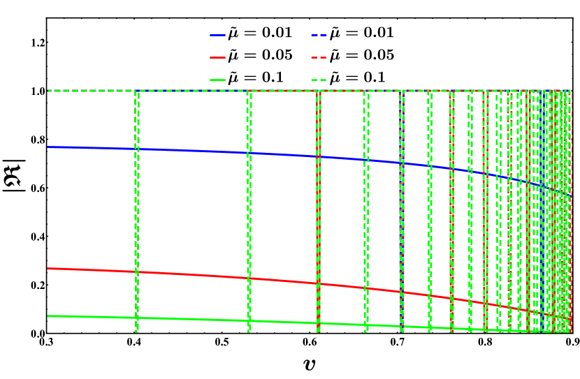
Figure 1: We have plotted the absolute values of the Boltzmann reflectivity (continuous curves) and the reflectivity of area-quantized BH (dashed curves) as a function of the velocity of the BH through the ultra-light boson environment. For both the quantum BHs, we have considered three different masses of the scalar field, $\tilde{\mu}\equiv\mu M=0.01$ (blue curve), $0.05$ (red curve) and $0.1$ (green curve). For all the plots, we have taken the dimensionless rotation parameter $\bar{a}\equiv(a/M)=0.2$.

The inspiral of quantum BHs through the DM environment emanates low-frequency GWs. Moreover, if the mass of the DM particles is $\mu$, a simple Lorentz transformation provides the following relation between frequency $\omega$ and velocity $v$ of the BH,

$$\omega=\frac{\mu}{\sqrt{1-v^{2}}}~{}.$$ (5)

Following this, in 1 we have plotted the absolute reflectivity $|\mathfrak{R}|$ for a Boltzmann reflective BH and an area-quantized BH with velocity for various masses of the ultra-light boson field. As evident, the reflectivity is dominant at low velocities, while for high velocities, the quantum BH behaves as a classical BH. This implies that we should look for quantum effects in the small-velocity regime, for which $\omega\gtrsim\mu$. Since the environmental effects are most important at low frequencies, it follows that ultra-light bosons are the best probes for excavating quantum effects at the BH horizon. This is true irrespective of the origin of such quantum effects.

Ultra-light boson environment — We have established that the best bet to detect the quantum nature of a BH horizon is through its motion in an environment consisting of ultra-light bosons of mass $\mu\sim 10^{-22}-10^{-10}$ eV. These bosons can be considered as scalar particles with mass $\mu$, being scattered by the quantum BH, giving rise to energy flux and dynamical friction, thereby slowing down the motion of the compact object. For BHs, such effects have been studied recently [62], here we wish to probe such effects for quantum BHs. Since generically, quantum BHs are endowed with a frequency-dependent reflectivity, we will present general results for the dynamical friction and energy flux due to scattering of any compact object with reflectivity by the ultra-light bosons. From these general results, true for any reflective object, we will specialize to the case of quantum BHs.

We model the environment with a massive complex scalar field $\Phi$ minimally coupled to gravity and satisfying the Klein-Gordon equation, $\Box\Phi=\mu^{2}\Phi$; the gravity sector satisfies Einstein’s equations. We choose the background geometry to be the stationary and axisymmetric Kerr metric and the following form for the scalar field:

$$\Phi=\sum_{l,m}e^{-i\left(\omega t-m\phi\right)}\Theta_{l}^{m}(\cos\theta)\mathcal{R}_{l}^{m}(r)~{},$$ (6)

where $\Theta{{}_{l}^{m}}(\cos\theta,\gamma^{2})$ is the angular part and $\mathcal{R}_{l}^{m}(r)$ denotes the radial part of the scalar perturbation. Upon substituing the scalar field ansatz into the field equation, the radial part $\mathcal{R}_{l}^{m}(r)$ satisfies the differential equation:

$$\Delta \frac{d}{dr}\left[\Delta\frac{d\mathcal{R}_{l}^{m}}{dr}\right]+\Big{[}\omega^{2}(r^{2}+a^{2})^{2}-4am\omega Mr$$

$$+(ma)^{2}-\left\{\lambda^{m}_{l}+\mu^{2}\Delta(r^{2}+a^{2})\right\}\Big{]}\mathcal{R}_{l}^{m}=0~{}.$$ (7)

Here, $\lambda^{m}_{l}$ are the eigenvalues associated with the angular function $\Theta{{}_{l}^{m}}(\cos\theta,\gamma^{2})$ and do not possess a closed analytical expression.

Solving the radial differential equation requires imposing appropriate boundary conditions at the surface of the ECO and asymptotic infinity. At spatial infinity, the radial function $\mathcal{R}_{l}^{m}$ becomes [62],

$$\mathcal{R}_{l}^{m}\simeq\frac{1}{r}\Big{[}I_{l}^{m}e^{-i\phi_{\infty}}+R_{l}^{m}e^{i\phi_{\infty}}\Big{]}~{},$$ (8)

where, $\phi_{\infty}\equiv k_{\infty}r-\eta\log(2k_{\infty}r)$, with $k_{\infty}\equiv\sqrt{\omega^{2}-\mu^{2}}$. Here, $I_{l}^{m}$ and $R_{l}^{m}$ are the respective amplitudes of the incident and the reflected waves and the quantity $\eta$ is defined as $\eta\equiv-M\{(\omega^{2}+k_{\infty}^{2})/k_{\infty}\}$. Going forward, we will only consider the case $\omega>\mu$, as otherwise, the scalar field would not allow wave-like solutions in the asymptotic limit. The incident amplitude $I_{l}^{m}$ can be determined by considering the ultra-light bosons to be scattered by the compact object; given a proper number density $n$ of ultra-light bosons coming from the direction $\bm{\xi}=-\cos\vartheta\partial_{z}+\sin\vartheta\partial_{y}$ [with $(x,y,z)$ being the asymptotic Cartesian coordinates], the amplitude is [62]

$$I_{l}^{m}=\frac{2l+1}{2k_{\infty}}\sqrt{\frac{\hbar n}{\mu}}\frac{(l-m)!}{(l+m)!}(-i)^{m+1}{P_{S}}_{l}^{m}(\cos\vartheta,\gamma^{2})~{}.$$ (9)

Here, ${P_{S}}_{l}^{m}(\cos\vartheta,\gamma^{2})$ are the oblate angular spheroidal harmonics. Unlike purely classical BHs, the quantum corrected BHs, (or general compact objects, for that matter), have both the in-going and the out-going waves at the near-horizon regime, related to each other by the reflectivity, which holds the key to the intrinsic properties of the compact object [58]. Thus, the radial perturbation variable $\mathcal{R}_{l}^{m}$ on the horizon reads,

$$\mathcal{R}_{l}^{m}\simeq\frac{1}{\sqrt{r^{2}+a^{2}}}\Big{[}T_{l}^{m}e^{-i\bar{\omega}r_{*}}+\mathbb{R}_{l}^{m}e^{i\bar{\omega}r_{*}}\Big{]}~{},$$ (10)

where $\bar{\omega}$ has been defined earlier. The ratio of the incoming and outgoing amplitude $(\mathbb{R}_{l}^{m}/T_{l}^{m})$ is proportional to the reflectivity of the compact object $\mathfrak{R}$, whose specific choice depends on the nature of the compact object.

Imprints in the inspiral phase — Having elaborated on the setting of the problem and the models of the quantum BHs we will focus on, in this section, we will provide the expressions for the energy flux and the imparted force due to scattering with the ultra-light boson environment.

Due to the stationarity of the background spacetime, it follows that the energy flux through the surface of the compact object is given by:

$$\dot{E}=\int_{\infty}T_{tr}~{}r^{2}\sin\theta d\theta d\phi,$$ (11)

As the ultra-light bosons scatter off the compact object, it will also feel a force due to momentum transfer from the bosons to the compact object. Using simple conservation laws, one can then calculate the force acting on the compact object  which yields:

$$F^{i}=-\int_{\infty}T^{ri}~{}r^{2}\sin\theta d\theta d\phi.$$ (12)

In both 11 and 12 (we refer to A for detailed derivation), one can use the stress-energy tensor components, namely $T_{tr}$ and $T^{ri}$ for the scalar field, to obtain the energy flux and the force in terms of the ratio of scattering amplitudes $\left(R^{m}_{l}/I^{m}_{l}\right)$ [62].

This ratio $\left(R^{m}_{l}/I^{m}_{l}\right)$ can be determined by solving the radial differential equation, as in Probing the quantum nature of black holes with ultra-light boson environments, with appropriate boundary conditions at the surface of the compact object. This is how the information about the nature of the compact object enters into the computation of the energy flux and the force. In general, the scattering amplitudes cannot be determined in a closed analytic form, however, the quantum aspects are best observed in the low-frequency regime ($\omega M\ll 1$), for which it is possible to obtain an analytic solution for the scattering amplitudes. We present these results below.

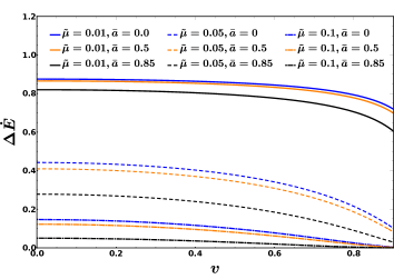
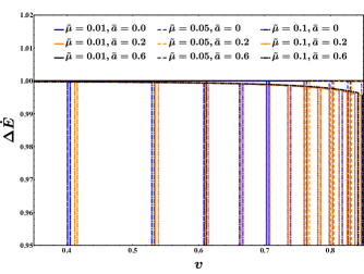
Figure 2: We have plotted $\Delta\dot{E}$ for BH with Boltzmann reflectivity on the left and area-quantized BH on the right, as a function of the speed of the BH, in the low-frequency ($\omega M\ll 1$) regime. The solid set of curves represents a scalar field DM of mass $\tilde{\mu}\equiv\mu M=0.01$, while the dashed and the dot-dashed sets of curves represent a scalar field DM of mass $\tilde{\mu}=0.05$ and $\tilde{\mu}=0.1$, respectively. Further, in each set, the three curves individually represent three different choices of the dimensionless rotation parameters $\bar{a}\equiv(a/M)=0.0$, $0.5$, and $0.85$. As evident, the energy flux for quantum BHs decrease, in comparison to that of classical BHs, by as large as $80\%$ for Boltmann reflective BHs, and by almost $100\%$ for area-quantized BHs.

This is achieved through the technique of matched asymptotic expansions [63, 64, 52], where one solves the radial equation in the near-horizon regime and at the asymptotic limit, separately. The arbitrary constants of integration are then fixed by imposing the respective boundary conditions 8 and 10 at infinity and the horizon. Finally, the large distance limit of the near-horizon solution is matched with the small distance limit of the asymptotic solution in the ‘matching’ region. In the low-frequency limit, it follows that $k_{\infty}a\sim(\omega M)(a/M)\ll 1$, implying $\lambda_{l}^{m}\simeq l(l+1)$, for the angular eigenvalues. Since the ‘matching’ region should be far from the horizon, but much smaller than the impact parameter $(l/k_{\infty})$ associated with the ultra-light bosons, the intermediate ‘matching’ region is defined as, $r_{+}\ll r\ll(l/k_{\infty})$. In this limit, we obtain the following ratio for the scattering amplitudes (the detailed derivation is provided in B)

$$\frac{R}{I} =-e^{2i\arg\Gamma(1+i\eta)}\Big{[}1-2\omega(r_{+}^{2}+a^{2})$$

$$\qquad\times e^{-\pi\eta}|\Gamma(1+i\eta)|^{2}k_{\infty}\left(\frac{1-\mathfrak{R}}{1+\mathfrak{R}}\right)\Big{]}\,.$$ (13)

Since all the modes with non-zero $l$ contribute at higher order in the frequency, the dominant contribution at low frequency arises from the $l=0$ mode, and hence $R$ and $I$ are the corresponding amplitudes. This is one of the main results of this paper. Given the above ratio of the scattering amplitude, we obtain the energy flux absorbed by the compact object at the leading order in the frequency, in its rest frame to read,

$$\dot{E} =\frac{\hbar n\omega^{2}}{\mu}\left(\frac{\pi\eta e^{-\pi\eta}}{\sinh(\pi\eta)}\right)A_{+}\,\textrm{Re}\left(\frac{1-\mathfrak{R}}{1+\mathfrak{R}}\right)\,.$$ (14)

Note that the energy flux of the ultra-light bosons depends on the reflectivity of the compact object at the leading order, and is proportional to the number density of the bosons as well as the area of the compact object. In the limit $\mathfrak{R}\to 0$, we get back previous results for BHs [62], while for a perfectly reflecting object, with $\mathfrak{R}=1$, the energy flux identically vanishes, as expected.

Finally, for the force, one rotates the reference frame so that the scalar wave is incident on the compact object  along $-\partial_{z^{\prime}}$, where the prime denotes the transformed coordinate system. In this transformed coordinate system $F^{x^{\prime}}=0$, $F^{y^{\prime}}=0$; at the leading order in the frequency, the force acting on the compact object may then be written as (refer to C for a detailed derivation),

$$\bm{F}=-\frac{4\pi\rho\bm{v}}{\mu^{2}v}\Biggl{\{}\eta^{2}\textrm{Re}\left[\psi(1+l_{\text{max}}+i\eta)-\psi(1+i\eta)\right]$$

$$+\frac{\omega k_{\infty}A_{+}}{4\pi}\left(\frac{\pi\eta e^{-\pi\eta}}{\sinh(\pi\eta)}\right)\textrm{Re}\left(\frac{1-\mathfrak{R}}{1+\mathfrak{R}}\right)\Biggr{\}}~{}.$$ (15)

Here, $\psi(z)$ is the di-gamma function, $\textbf{v}=\bm{\partial}_{\bf z^{\prime}}(k_{\infty}/\omega)$ is the relative velocity of the compact object with respect to an asymptotic observer, and $l_{\rm max}$ is a cutoff, necessary to avoid a Logarithmic divergence in $l$. Note that, the force on the compact object also depends on the reflectivity at the leading order of the frequency. Further, the force is proportional to the velocity and hence is indeed a frictional force.

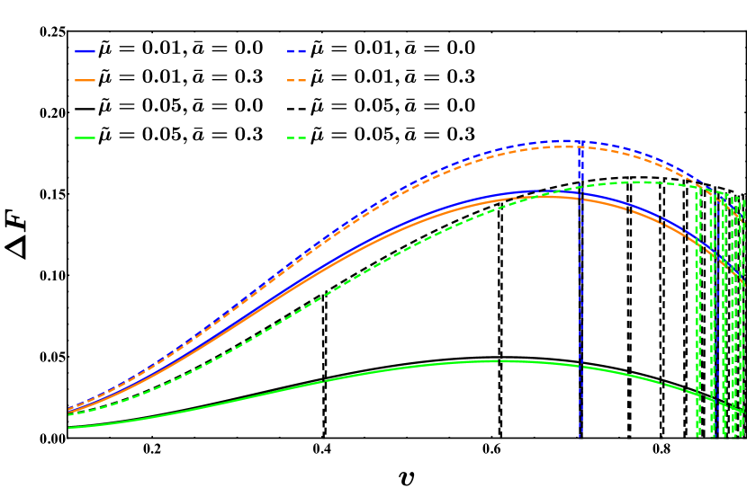
Figure 3: Plot of the fractional force $\Delta\bm{F}$ against the velocity of the quantum BH has been depicted. The continuous curves depict the case of Boltzmann reflective BH, and the dashed curves are for the area-quantized BH (with $\alpha=2$). It is clear that for a given velocity, the difference in the force is larger for the area-quantized BH, as it has larger reflectivity at smaller velocities. We have considered two different DM masses $\tilde{\mu}\equiv\mu M$ = 0.01, and 0.05, along with two different dimensionless rotation parameters $\bar{a}\equiv(a/M)=0.0$, $0.3$. As evident, for small velocities, quantum BHs experience a force larger than the classical BHs by at max $20\%$.

The difference between a quantum and classical BH can be illustrated with the following two observables,

$$\Delta\dot{E}=\frac{\dot{E}_{\rm BH}-\dot{E}_{\rm QBH}}{\dot{E}_{\rm BH}}~{};\qquad\Delta\bm{F}=\frac{\bm{F}_{\rm QBH}-\bm{F}_{\rm BH}}{|\bm{F}_{\rm BH}|}~{}.$$ (16)

Both of these have been depicted as a function of the relative velocity $v$ of the quantum BH with respect to the DM environment, for three choices of the DM masses, in the low-frequency regime. The fractional energy flux has been depicted in 2, while the fractional force has been illustrated in 3 for both the Boltzmann reflective BH and for an area-quantized BH. Intriguingly, as evident from 2 the energy absorbed by a BH with Boltzmann reflectivity can be decrease by $80\%$, while the force can increase by $15\%$ in comparison to that of a classical BH. For an area quantized BH, on the other hand, the energy decrease can be almost $100\%$, while the force can increase by at most $20\%$ in comparison to the classical BH. If the mass of the scalar field increases, the difference from a classical BH significantly decreases for a Boltzmann reflective BH, while for the area-quantized case, it remains almost identical. Thus energy absorption in an ultra-light DM environment can provide a tell-tale signature of the quantum nature of BHs.

The above expressions have been derived in the rest frame of the compact object, while in a typical astrophysical scenario, the compact object will not be stationary, but the environment consisting of ultra-light bosons will be. Therefore, the energy flux and the force experienced by the compact object should be transformed to the frame of the ultra-light bosons, which is achieved by Lorentz transformation, yielding,

$$\dot{E}^{\prime}=\dot{E}+\textbf{v}\cdot\textbf{F}~{};\qquad\textbf{F}^{\prime}=\textbf{F}+\textbf{v}\dot{E}~{}.$$ (17)

Due to the mixing between the energy flux and the force between the two frames of reference, both the energy flux and the force in the DM frame will depend on the reflectivity. In particular, the excess energy at infinity due to scattering of the ultra-light scalars from the compact object, is given by $\dot{E}^{\prime}$, as seen by an asymptotic observer. Therefore, the energy flux at infinity modifies to [54],

$$\dot{E}_{\rm GW}\rightarrow\left(1+\frac{\dot{E}^{\prime}}{\dot{E}_{\rm GW}}\right)\dot{E}_{\rm GW}~{}.$$ (18)

Since we wish to distinguish a quantum BH from a classical BH, it is instructive to consider the following difference $\dot{E}^{\prime}_{\rm BH}-\dot{E}^{\prime}_{\rm QBH}$, which contributes to the change in the GW flux at infinity due to the quantum nature of BHs.

As the presence of non-trivial reflectivity will affect the energy absorbed by the quantum BHs, in particular, it will decrease the absorbed energy flux when compared to a classical BH. This is expected, as a classical BH engulfs everything thrown at it, while a quantum BH reflects most of it back. As a consequence, in the extreme mass ratio system, we expect a change in the number of cycles the secondary BH performs around the primary, which can lead to observable effects. In particular, if the change in the number of cycles satisfy $\Delta\mathcal{N}_{\rm cycles}\gtrsim 1$, it is expected that the corresponding effect can be observed. As 1 clearly demonstrates, for both Boltzmann reflective and area-quantized BHs, $\Delta\mathcal{N}_{\rm cycles}\gtrsim 1$, due to the quantum nature of these BHs, provided the environment consists of DM particles having mass $\lesssim 10^{-13}$ eV. Also change in the number of cycles are different for Boltzmann reflective BH when compared to the area-quantized BH. This implies that, not only quantum nature of BHs, but also specific models of quantum BHs can be tested using an environment consisting of ultra-light DM particles.

Nature of	Mass of	$\Delta\mathcal{N}_{\rm cycles}$
Quantum BH	DM (in eV)
Boltzmann	$1.5\times 10^{-14}$	$\sim 9$
Reflectivity	$0.75\times 10^{-13}$	$\sim 1$
	$1.5\times 10^{-13}$	$<1$
Area-quantized	$1.5\times 10^{-14}$	$\sim 11$
BH	$0.75\times 10^{-13}$	$\sim 3$
	$1.5\times 10^{-13}$	$<1$

Table 1: We present the change in the number of cycles of an extreme mass ratio system, with the mass of the secondary being $M=10^{2}M_{\odot}$, due to the quantum nature of BHs. As evident, for BHs with Boltzmann reflectivity moving in an environment with DM particles having masses $\lesssim 10^{-13}$ eV, the change in the number of cycles is $\Delta\mathcal{N}_{\rm cycles}\gtrsim 1$. The situation is identical for the area-quantized BH. However, the change in the number of cycles, for a given DM mass is higher for the area-quantized BH, due to its perfectly reflecting nature.

Discussion — In this letter we have proposed a tantalizing new method of probing various quantum corrections to a BH, using the energy absorption and the frictional force experienced by the BH, as it moves through a ultralight scalar environment. Such an environment, which can act as DM halo, is supposed to be ubiquitous and must be present surrounding any BH spacetime. Specifically, for the extreme mass ratio binary systems, such environmental effect comes naturally into consideration as the motion of the secondary BH around the primary is considered. In particular, any deviation from the BH nature is going to modify the number of cycles the secondary passes through while orbiting the primary and is a potential observable. Following which we have computed the energy absorbed and force experienced by a quantum BH as it moves through a DM environment consisting of ultra-light bosons. Owing to the reflective nature of the horizon for the quantum BHs, the energy flux across the horizon decreases, while the damping force increases, in comparison to a classical BH, with the percentage change depending on the mass of the DM particles in the environment. For an environment consisting of DM particles with mass $\lesssim 10^{-13}$ eV, the change in energy flux for a BH with Boltzmann reflectivity can be as large as eighty percent of the flux received by a classical BH. While the change in force becomes as large as fifteen percent. For an area quantized BH, due to its perfectly reflecting nature in most of the frequencies, the change in energy flux is almost hundred percent, while the change in force is about twenty percent at max, when compared to a classical BH. As a consequence the number of cycles experienced by a secondary BH orbiting the primary is going to be modified due to the effect of the environment, and we have shown that $\Delta\mathcal{N}_{\rm cycles}\gtrsim 1$, for DM masses $\lesssim 10^{-13}$ eV, irrespective of the details of the quantum nature of the BH horizon. Thus through the next generation of GW detectors, e.g., LISA, we will be able to probe indelible signature in the GW waveform which can then be used to differentiate such objects from a classical BH. This result paves the road for future works on probes of such compact objects and their underlying fundamental physics using environmental effect of GW.

Appendix A Energy and momentum in asymptotically flat spacetimes

Here, we intend to provide some justification for the energy loss and force formulas employed in the main body of this article. A justification was originally provided in [65], however, that derivation is based on pseudotensorial quantities; here we briefly describe a tensorial generalization of that approach (based on the formalism developed in [66] and [67]) in which the meaning of the pseudotensorial quantities is elucidated.

We begin by introducing a flat background metric $\bar{g}_{\mu\nu}$, and in this appendix, we employ the convention that indices are raised and lowered using $\bar{g}_{\mu\nu}$ and define $\hat{g}^{\mu\nu}$ to be the inverse of the dynamical metric $g_{\mu\nu}$ (we do not assume the usual Cartesian $\eta_{\cdot\cdot}=\text{diag}(-1,1,1,1)$ form, and permit curvilinear coordinates). We also introduce a compatible torsion-free reference connection $\bar{\nabla}$ with connection coefficients $\bar{\Gamma}{{}^{\lambda}}{{}_{\mu\nu}}$. One can construct the following tensorial quantities:

$$W{{}^{\lambda}}{{}_{\mu\nu}} :={\Gamma}{{}^{\lambda}}{{}_{\mu\nu}}-\bar{\Gamma}{{}^{\lambda}}{{}_{\mu\nu}}$$ (19)

$$W^{\mu} :=\hat{g}^{\sigma\tau}W{{}^{\mu}}{{}_{\sigma\tau}}-\hat{g}^{\mu\sigma}W{{}^{\nu}}{{}_{\nu\sigma}}~{},$$ (20)

which can be used to construct the following first-order action (cf. Eq. (28) in [67]):

$$S_{GR} =\frac{1}{2\kappa}\int_{U}d\mu\left[{R}-{\nabla}_{\mu}W^{\mu}\right]$$ (21)

$$=\frac{1}{2\kappa}\int_{U}d\mu\left(W{{}^{\mu}}_{\sigma\lambda}W{{}^{\lambda}}{{}_{\mu\tau}}-W{{}^{\nu}}_{\sigma\tau}W{{}^{\lambda}}{{}_{\lambda\nu}}\right)\hat{g}^{\sigma\tau}~{},$$

where $d\mu:=\sqrt{|g|}d\underline{\mu}$, $\kappa=8\pi G$, and the flatness of the background metric $\bar{g}_{\mu\nu}$ has been employed. Given a vector $\xi^{\mu}$ which is covariantly constant with respect to $\bar{g}_{\mu\nu}$ (namely, $\bar{\nabla}_{\nu}\xi^{\mu}=0$), the following current:

$$J^{\mu}= \xi^{\beta}\left[2G_{\nu\beta}\,\hat{g}^{\mu\nu}-{{}_{\rm E}}\Theta{{}^{\mu}}{{}_{\beta}}\right]~{},$$ (22)

identically satisfies $\partial_{\mu}(\sqrt{|g|}J^{\mu})=0$ (by way of the Katz-Ori identity [66]). The current can can be thought of as an energy density current for timelike $\xi^{\mu}$, and as a momentum density current for spacelike $\xi^{\mu}$, and one can replace the Einstein tensor using the Einstein equation $G_{\mu\nu}=\kappa T_{\mu\nu}$. The quantity ${{}_{E}}\Theta{{}^{\alpha}}{{}_{\beta}}$ is a tensorial generalization of the Einstein (canonical energy-momentum) pseudotensor:

$${{}_{E}}\Theta{{}^{\alpha}}{{}_{\beta}}= -W^{\alpha}W{{}^{\sigma}}_{\sigma\beta}-\left[W{{}^{\alpha}}{{}_{\beta\sigma}}\hat{g}^{\sigma\tau}+W{{}^{\tau}}{{}_{\beta\sigma}}\hat{g}^{\alpha\sigma}\right]W{{}^{\nu}}_{\nu\tau}$$

$$+\left[W^{\sigma}{{}_{\beta\nu}}\hat{g}^{\nu\tau}+W^{\tau}{{}_{\beta\nu}}\hat{g}^{\nu\sigma}\right]W^{\alpha}{{}_{\sigma\tau}}$$

$$-\delta{{}^{\alpha}}{{}_{\beta}}\left[{R}-{\nabla}_{\sigma}W^{\sigma}\right]~{}.$$ (23)

From A, one can see that the ${{}_{E}}\Theta{{}^{\alpha}}{{}_{\beta}}$ shifts the pseudotensorial ambiguities of the Einstein pseudotensor to the choice of coordinates on the flat reference geometry used to construct $\bar{\Gamma}{{}^{\lambda}}{{}_{\mu\nu}}$. A detailed discussion of this point can be found in [67].

Now for convenience, one can define $\bar{J}^{\mu}:=\Psi J^{\mu}$, where $\Psi:=\sqrt{|g/\bar{g}|}$. Now what is particularly useful is the fact that the current $\bar{J}^{\mu}$ can be clearly split into a gravitational part and a nongravitational part $\bar{J}^{\mu}=\bar{J}_{M}^{\mu}+\bar{J}_{G}^{\mu}$ where:

$$\bar{J}_{M}^{\mu}=\,2\kappa\Psi\xi^{\beta}T_{\nu\beta}\,\hat{g}^{\mu\nu}~{};\qquad\bar{J}_{G}^{\mu}=\,-\Psi\xi^{\beta}{{}_{\rm E}}\Theta{{}^{\mu}}{{}_{\beta}}~{}.$$ (24)

From the divergence theorem, one can derive the following expression for a divergence-free current satisfying $\bar{\nabla}_{\mu}\bar{J}^{\mu}=0$:

$$\partial_{t}\int_{\Sigma_{t}}d\bar{\Sigma}_{\mu}\bar{J}^{\mu}=-\int_{\partial\Sigma_{t}}d\bar{\sigma}r_{\mu}\bar{J}^{\mu}~{},$$ (25)

where $d\bar{\Sigma}_{\mu}$ is the directed surface element on $\Sigma_{t}$, and $d\bar{\sigma}$ is the surface element on $\partial\Sigma_{t}$ (both defined with respect to $\sqrt{|\bar{g}|}$), with $r^{\mu}$ is a unit vector tangent to $\Sigma_{t}$ and normal to $\partial\Sigma_{t}$. The derivation is straightforward, and follows that found in [65]. One may rewrite 25 as:

$$\partial_{t}\int_{\Sigma_{t}}d\bar{\Sigma}_{\mu}\bar{J}_{M}^{\mu} +\partial_{t}\int_{\Sigma_{t}}d\bar{\Sigma}_{\mu}\bar{J}_{G}^{\mu}$$

$$=-\int_{\partial\Sigma_{t}}d\bar{\sigma}r_{\mu}\bar{J}_{M}^{\mu}-\int_{\partial\Sigma_{t}}d\bar{\sigma}r_{\mu}\bar{J}_{G}^{\mu}~{}.$$

We consider a steady state energy-momentum tensor, and coordinates in which $g_{\mu\nu}$ is stationary, and it follows that:

$$\partial_{t}\int_{\Sigma_{t}}d\bar{\Sigma}_{\mu}\bar{J}_{M}^{\mu}=0~{},$$ (26)

and one has the expression:

$$\partial_{t}\int_{\Sigma_{t}}d\bar{\Sigma}_{\mu}\bar{J}_{G}^{\mu}=\, -\int_{\partial\Sigma_{t}}d\bar{\sigma}r_{\mu}\bar{J}_{M}^{\mu}-\int_{\partial\Sigma_{t}}d\bar{\sigma}r_{\mu}\bar{J}_{G}^{\mu}~{}.$$

The left hand side of the above can be interpreted as the time derivative of the integrated energy density for timelike $\xi^{\mu}$ and a force for spacelike $\xi^{\mu}$; in both cases, the evaluation consists of a surface integral over $\partial\Sigma_{t}$.

In an asymptotically flat spacetime, one can evaluate the surface integral in the vicinity of spatial infinity $\partial\Sigma_{t}\rightarrow i_{0}$, treating deviations from flat spacetime (in some appropriate coordinate gauge) as perturbations. Assuming $T_{\mu\nu}\sim O(\epsilon)$ and $g_{\mu\nu}-\bar{g}_{\mu\nu}\sim{W^{\sigma}}_{\mu\nu}\sim O(\epsilon)$, one finds that to $O(\epsilon)$

$$\bar{J}_{M}^{\mu}\approx\,2\kappa T{{}^{\mu}}{{}_{\nu}}\xi^{\nu},\qquad\qquad\bar{J}_{G}^{\mu}\approx\,0~{},$$ (27)

and it follows that

$$\partial_{t}\int_{\Sigma_{t}}d\bar{\Sigma}_{\mu}\bar{J}_{G}^{\mu}\approx\, -2\kappa\int_{\partial\Sigma_{t}}d\bar{\sigma}r_{\mu}T{{}^{\mu}}{{}_{\nu}}\xi^{\nu}~{}.$$ (28)

Note that to $O(\epsilon)$, the quantity $W{{}^{\lambda}}_{\mu\nu}$ does not appear, and the only dependence on the background coordinate gauge arises through the surface element $d\bar{\sigma}$.

As discussed right after 22, the current $J^{\mu}$ represents an energy density current for timelike $\xi^{\mu}$ and a momentum current for spacelike $\xi^{\mu}$. Given 26, and 25, one can use 28 and the choice of coordinate basis vectors $\partial_{t}$ and $\partial_{i}$ to obtain the results:

$$\partial_{t}E\approx\, -2\kappa\int_{\partial\Sigma_{t}}d\bar{\sigma}r_{\mu}T{{}^{\mu}}{{}_{t}}~{},$$ (29)

and

$$F^{i}:=\partial_{t}P^{i}\approx\, -2\kappa\int_{\partial\Sigma_{t}}d\bar{\sigma}r_{\mu}T{{}^{\mu}}{{}_{i}}~{},$$ (30)

which we employ in the main text.

Appendix B Scattering amplitudes in the low-frequency regime

In this appendix, we will provide the explicit calculation of the scattering amplitude $(R^{m}_{l}/I^{m}_{l})$ in low frequency approximation using matched asymptotic expansion technique, as mentioned in the main letter.

B.0.1 Scalar perturbation in the near horizon region

We will start by solving the radial perturbation equation, presented in Probing the quantum nature of black holes with ultra-light boson environments,in the near-horizon regime. For this purpose, it is useful to employ a change of the radial coordinate,

$$x\equiv\frac{r-r_{+}}{r_{+}-r_{-}}\ll\frac{l+1}{\omega(r_{+}-r_{-})}~{},$$ (31)

which is dimensionless and the inequality simply follows from the fact that near the horizon $x\ll 1$ and in the small-frequency approximation $\omega(r_{+}-r_{-})\ll 1$, as well. In terms of this new dimensionless radial coordinate, the radial perturbation equation becomes,

$$x(x+1) \frac{d}{dx}\left[x(x+1)\frac{d}{dx}\mathcal{R}_{l}^{m~{}\textrm{(nh)}}\right]$$

$$+\left[Q^{2}-l(l+1)x(x+1)\right]\mathcal{R}_{l}^{m~{}\textrm{(nh)}}=0~{},$$ (32)

where we have defined,

$$Q \equiv\frac{r_{+}^{2}+a^{2}}{r_{+}-r_{-}}\left(m\Omega_{H}-\omega\right)~{},$$ (33)

and $\mathcal{R}_{l}^{m~{}\textrm{(nh)}}$ is the radial perturbation in the near-horizon region. The general solution of B.0.1 is given in terms of hypergeometric functions [68],

$$\mathcal{R}_{l}^{m~{}\textrm{(nh)}}=\left(1+x\right)^{iQ}$$

$$\times\bigg{\{}c_{1}x^{-iQ}\,_{2}F_{1}(-l,l+1;1-2iQ;-x)$$

$$+c_{2}x^{iQ}\,_{2}F_{1}(-l+2iQ,l+1+2iQ;1+2iQ;-x)\bigg{\}}~{}.$$ (34)

The arbitrary constants $c_{1}$ and $c_{2}$ are to be fixed by taking the small $x$ limit of the above solution and matching it with the physical boundary condition at the horizon given in 10. In this limit, hypergeometric functions can be expanded to obtain a power law solution,

$$\mathcal{R}_{l}^{m~{}\textrm{(nh)}}\Big{|}_{\rm near}=c_{1}x^{-iQ}+c_{2}x^{iQ}~{}.$$ (35)

Noting that $\mathcal{R}_{l}^{m}=(r_{+}^{2}+a^{2})^{-1/2}\Psi_{l}^{m}$, in the near horizon limit, as well as the fact that $Q\ln x=-(\omega-m\Omega_{\rm h})r_{*}$, a comparison of 35 with 10, yields,

$$c_{1}=\frac{\mathbb{R}_{l}^{m}}{\sqrt{r_{+}^{2}+a^{2}}}~{};\qquad c_{2}=\frac{T_{l}^{m}}{\sqrt{r_{+}^{2}+a^{2}}}~{}.$$ (36)

The BH scenario can be obtained from our results by simply substituting the surface reflectivity $\mathbb{R}_{l}^{m}$ of the ECO to be zero, implying $c_{1}=0$. In what follows we will keep the results as general as possible and are not going to assume any particular form of the reflectivity, by keeping both $c_{1}$ and $c_{2}$ explicitly in our calculations.

Having discussed the near-horizon behaviour of the near-horizon solution, we consider now the extension of the near-horizon solution to the intermediate region, which is obtained by taking the $x\gg 1$ limit of B.0.1. Therefore, expanding the hypergeometric functions for large values of $x$ and keeping only the leading order terms, we obtain [63, 52],

$$\mathcal{R}_{l}^{m~{}\textrm{(nh)}}\Big{|}_{\rm far} \simeq d_{1}x^{l}+\left(\frac{d_{2}}{2l+1}\right)x^{-l-1}~{}.$$ (37)

Here we have denoted the coefficients of the terms $x^{l}$ and $x^{-l-1}$ are by $d_{1}$ and $d_{2}$ and can be expressed in terms of $c_{1}$ and $c_{2}$ as,

$$d_{1} =\frac{\Gamma(2l+1)}{\Gamma(l+1)}\left[c_{1}\frac{\Gamma(1-2iQ)}{\Gamma(l+1-2iQ)}+c_{2}\frac{\Gamma(1+2iQ)}{\Gamma(l+1+2iQ)}\right]~{},$$ (38)

$$d_{2} =(2l+1)\frac{\Gamma(-2l-1)}{\Gamma(-l)}\left[c_{1}\frac{\Gamma(1-2iQ)}{\Gamma(-l-2iQ)}+c_{2}\frac{\Gamma(1+2iQ)}{\Gamma(-l+2iQ)}\right]~{}.$$ (39)

The following identities can be used to suitably express the ratio of the gamma functions in terms of Pochhammer symbol,

$$\frac{\Gamma(1-2iQ)}{\Gamma(l+1-2iQ)} =\frac{1}{(l-2iQ)(l-1-2iQ)\cdots(1-2iQ)}=\frac{1}{(1-2iQ)_{l}}~{}.$$ (40)

Similarly, it also follows that,

$$\frac{\Gamma(1+2iQ)}{\Gamma(l+1+2iQ)} =\frac{1}{(2iQ+l)(2iQ+l-1)\cdots(2iQ+1)}=\frac{1}{(2iQ+1)_{l}}~{},$$ (41)

$$\frac{\Gamma(1-2iQ)}{\Gamma(-l-2iQ)} =(-2iQ)(-1-2iQ)\cdots(-l-2iQ)=(-1)^{l+1}\left(2iQ\right)_{l+1}~{},$$ (42)

$$\frac{\Gamma(1+2iQ)}{\Gamma(-l+2iQ)} =(2iQ)(-1+2iQ)\cdots(-l+2iQ)=(2iQ-l)_{l+1}~{}.$$ (43)

where, the Pochhammer symbol is defined as, $(x)_{n}=x(x+1)(x+2)\cdots(x+n-1)$.

These results along with 36 lets us express $d_{1}$ and $d_{2}$ in terms of the reflection and transmission coefficients associated with the surface of the ECO as,

$$d_{1} =\frac{(2l)!}{l!}\frac{1}{\sqrt{r_{+}^{2}+a^{2}}}\left[\frac{\mathbb{R}_{l}^{m}}{(1-2iQ)_{l}}+\frac{T_{l}^{m}}{(1+2iQ)_{l}}\right]~{},$$ (44)

$$d_{2} =\frac{(-1)^{l+1}}{2}\frac{l!}{(2l)!}\frac{1}{\sqrt{r_{+}^{2}+a^{2}}}\Big{[}\mathbb{R}_{l}^{m}(-l-2iQ)_{l+1}+T_{l}^{m}(2iQ-l)_{l+1}\Big{]}~{},$$ (45)

Note that we also have the following result: $(-l-2iQ)_{l+1}=(-l-2iQ)\cdots(-2iQ)=(-1)^{l+1}(2iQ)_{l+1}$, and hence the above coefficients can also be expressed in various other forms. Further, in the BH limit ($\mathbb{R}_{l}^{m}\to 0$), the above solution reduces to the one in [62].

In the intermediate region, with $x\gg 1$, we can effectively express the re-scaled radial coordinate as follows, $x\simeq\{r/(r_{+}-r_{-}\}$, such that we can rewrite the near-horizon solution in the matching region as,

$$\mathcal{R}_{l}^{m~{}\textrm{(nh)}}\Big{|}_{\rm far}\approx\left(\frac{d_{1}}{(r_{+}-r_{-})^{l}}\right)r^{l}+\left(\frac{d_{2}}{(r_{+}-r_{-})^{-l-1}}\right)r^{-l-1}\,.$$ (46)

We will be using this result extensively to match with the far zone solution, which we will now derive.

B.0.2 Scalar perturbation in the asymptotic region

In this section, we will present the solution to the radial part of the scalar perturbation in the asymptotic region, which corresponds to $r\gg r_{+}$. In this limit, Probing the quantum nature of black holes with ultra-light boson environments simplifies to,

$$\left[\frac{d^{2}}{dr^{2}}+k_{\infty}^{2}-\frac{2\eta k_{\infty}}{r}-\frac{l(l+1)}{r^{2}}\right]\left(\sqrt{\Delta}\,\mathcal{R}_{l}^{m~{}\textrm{(asy)}}\right)=0~{}.$$ (47)

The general solutions to the above equation is given in terms of Coulomb wave functions [69],

$$\mathcal{R}_{l}^{m~{}\textrm{(asy)}}=\frac{c_{3}}{r}\,\text{F}_{l}^{C}(\eta,k_{\infty}r)+\frac{c_{4}}{r}\,\text{G}_{l}^{C}(\eta,k_{\infty}r)~{}.$$ (48)

Now we need to match this asymptotic solution with the near-horizon solution in the intermediate zone. For this purpose, we expand the Coulomb functions in the limit $k_{\infty}r\ll l$ (which corresponds to the radial parameter being small compared to the impact parameter), and one recovers,

$$\mathcal{R}_{l}^{m~{}\textrm{(asy)}}\Big{|}_{\rm near} \simeq c_{3}C_{l}(\eta)k_{\infty}^{l+1}\,r^{l}$$

$$+c_{4}\left(\frac{k_{\infty}^{-l}}{(2l+1)C_{l}(\eta)}\right)\,r^{-l-1}~{},$$ (49)

where we have introduced the constant $C_{l}(\eta)$, having the following expression,

$$C_{l}(\eta)=\frac{2^{l}e^{-\eta\pi/2}|\Gamma(l+1+i\eta)|}{(2l+1)!}~{}.$$ (50)

The large $r$ limit of the near-horizon solution, presented in 46, and the small $r$ limit of the asymptotic solution, as discussed in B.0.2, must be matched to one another. This relates the arbitrary constants $c_{3}$ and $c_{4}$ to $d_{1}$ and $d_{2}$, such that,

$$c_{3} =\frac{d_{1}}{C_{l}(\eta)k_{\infty}^{l+1}(r_{+}-r_{-})^{l}}~{},$$ (51)

$$c_{4} =\frac{d_{2}C_{l}(\eta)}{k_{\infty}^{-l}(r_{+}-r_{-})^{-l-1}}~{}.$$ (52)

Thus, we have related the near-horizon boundary condition to the asymptotic solution, and finally, to obtain the scattering amplitude $(R_{l}^{m}/I_{l}^{m})$ in terms of properties in the near-horizon regime, we must relate the coefficients $c_{3}$ and $c_{4}$ with the physical boundary condition at infinity. For this purpose, we need to consider the $k_{\infty}r\to\infty$ limit of the asymptotic solution in 48, which gives,

$$\mathcal{R}_{l}^{m~{}\textrm{(asy)}}\Big{|}_{\rm far} \simeq\frac{c_{3}}{r}\sin[\theta_{l}(\eta,k_{\infty}r)]$$

$$+\frac{c_{4}}{r}\cos[\theta_{l}(\eta,k_{\infty}r)]\,.$$ (53)

Here, $\theta_{l}\equiv k_{\infty}r-\eta\log(2k_{\infty}r)-l(\pi/2)+\arg\Gamma(l+1+i\eta)$, where, $\arg(z)$ denotes the principal argument of the complex quantity $z$. Expanding out the $\sin$ and $\cos$ in terms of exponentials and using the asymptotic boundary condition, as in 8, we obtain,

$$R_{l}^{m}=\left(\frac{c_{4}-ic_{3}}{2}\right)e^{-iA}~{},\quad I_{l}^{m}=\left(\frac{c_{4}+ic_{3}}{2}\right)e^{iA}\,.$$ (54)

where, we have defined $A\equiv(l\pi/2)-\arg\left[\Gamma(l+1+i\eta)\right]$ with $l$ taking integer values.

B.0.3 Matching region and scattering amplitudes

Having derived all the relevant limits of the near-horizon and the asymptotic solutions, we wish to determine the scattering amplitudes by matching them appropriately. Note that the asymptotic amplitudes are dependent on the constants $c_{3}$ and $c_{4}$, which are dependent on the near-horizon quantities $d_{1}$ and $d_{2}$ through 52, and to the horizon reflectivity by 44 and 45, respectively. To obtain the scattering amplitude, we start by noting, $e^{-il\pi}=(-1)^{l}$, for integer values of $l$, which lets us obtain,

$$e^{-2iA}=e^{-i[l\pi-2\arg\Gamma(l+1+i\eta)]}=(-1)^{l}e^{2i\arg\Gamma(l+1+i\eta)}~{}.$$ (55)

Using this result for $e^{-2iA}$, along with 52 and 54, we obtain the following ratio between the scattering amplitudes, for generic choices of the angular momentum $l$,

$$\frac{R_{l}^{m}}{I_{l}^{m}}=e^{-2iA}\frac{c_{4}-ic_{3}}{c_{4}+ic_{3}}$$

$$=(-1)^{l}e^{2i\arg\Gamma(l+1+i\eta)}\frac{c_{4}-ic_{3}}{c_{4}+ic_{3}}$$

$$=(-1)^{l}e^{2i\arg\Gamma(l+1+i\eta)}\frac{z_{l}\frac{d_{2}}{d_{1}}-i}{z_{l}\frac{d_{2}}{d_{1}}+i}$$

$$=(-1)^{l}e^{2i\arg\Gamma(l+1+i\eta)}$$

$$\times\Bigg{[}\frac{(l!)^{2}\,z_{l}\bigg{\{}(2iQ)_{l+1}^{2}(2iQ-l)_{l+1}c_{1}+(-1)^{l+1}(2iQ)_{l+1}(2iQ-l)^{2}_{l+1}c_{2}\bigg{\}}+4\,(2l!)^{2}\,Q\bigg{\{}(-1)^{l}(2iQ)_{l+1}c_{1}+(2iQ-l)_{l+1}c_{2}\bigg{\}}}{(l!)^{2}\,z_{l}\bigg{\{}(2iQ)_{l+1}^{2}(2iQ-l)_{l+1}c_{1}+(-1)^{l+1}(2iQ)_{l+1}(2iQ-l)^{2}_{l+1}c_{2}\bigg{\}}-4\,(2l!)^{2}\,Q\bigg{\{}(-1)^{l}(2iQ)_{l+1}c_{1}+(2iQ-l)_{l+1}c_{2}\bigg{\}}}\Bigg{]}$$

$$=(-1)^{l+1}e^{2i\arg\Gamma(1+l+i\eta)}\Bigg{[}\frac{\frac{\mathbb{R}_{l}^{m}}{T_{l}^{m}}(1+2iQ)_{l}\bigg{\{}(2l)!^{2}-(l!)^{2}z_{l}Q|(1+2iQ)_{l}|^{2}\bigg{\}}+(1-2iQ)_{l}\Bigg{\{}(2l)!^{2}+(l!)^{2}z_{l}Q|(1+2iQ)_{l}|^{2}\bigg{\}}}{\frac{\mathbb{R}_{l}^{m}}{T_{l}^{m}}(1+2iQ)_{l}\bigg{\{}(2l)!^{2}+(l!)^{2}z_{l}Q|(1+2iQ)_{l}|^{2}\bigg{\}}+(1-2iQ)_{l}\bigg{\{}(2l)!^{2}-(l!)^{2}z_{l}Q|(1+2iQ)_{l}|^{2}\bigg{\}}}\Bigg{]}$$

$$=(-1)^{l+1}e^{2i\arg\Gamma(1+l+i\eta)}\Bigg{[}\frac{\frac{\mathbb{R}_{l}^{m}}{T_{l}^{m}}\left\{1-\left(\frac{(l!)}{(2l)!}\right)^{2}z_{l}Q|(1+2iQ)_{l}|^{2}\right\}+\frac{(1-2iQ)_{l}}{(1+2iQ)_{l}}\left\{1+\left(\frac{(l!)}{(2l)!}\right)^{2}z_{l}Q|(1+2iQ)_{l}|^{2}\right\}}{\frac{\mathbb{R}_{l}^{m}}{T_{l}^{m}}\left\{1+\left(\frac{(l!)}{(2l)!}\right)^{2}z_{l}Q|(1+2iQ)_{l}|^{2}\right\}+\frac{(1-2iQ)_{l}}{(1+2iQ)_{l}}\left\{1-\left(\frac{(l!)}{(2l)!}\right)^{2}z_{l}Q|(1+2iQ)_{l}|^{2}\right\}}\Bigg{]}$$

$$=(-1)^{l+1}e^{2i\arg\Gamma(1+l+i\eta)}\left[\frac{(1+\mathfrak{R})+\left(\frac{(l!)}{(2l)!}\right)^{2}z_{l}Q|(1+\bar{Q})_{l}|^{2}(1-\mathfrak{R})}{(1+\mathfrak{R})-\left(\frac{(l!)}{(2l)!}\right)^{2}z_{l}Q|(1+\bar{Q})_{l}|^{2}(1-\mathfrak{R})}\right]~{}.$$ (56)

Note that in the above expression we have defined the effective reflectivity $\mathfrak{R}$ as the multiplication of the ratio $(\mathbb{R}_{l}^{m}/T_{l}^{m})$ with the ratio of Pochhammer symbols $\{(1+2iQ)_{l}/(1-2iQ)_{l}\}$ given by,

$$\mathfrak{R}\equiv\frac{\left(1+2iQ\right)_{l}}{\left(1-2iQ\right)_{l}}\frac{\mathbb{R}_{l}^{m}}{T_{l}^{m}}~{}.$$ (57)

Moreover, we have used the following expression for the quantity $z_{l}$,

$$z_{l}=C_{l}(\eta)^{2}k_{\infty}^{2l+1}(r_{+}-r_{-})^{2l+1}~{},$$ (58)

along with the fact that $(r_{+}-r_{-})=2\sqrt{M^{2}-a^{2}}$. Putting the explicit expressions and after some manipulation, one can finally obtain the scattering amplitude,

$$\frac{R_{l}^{m}}{I_{l}^{m}} =(-1)^{l+1}e^{2i\arg\Gamma(1+l+i\eta)}\Bigg{[}\frac{1+\frac{(l!)^{2}}{(2l!)^{2}}QC_{l}(\eta)^{2}|(1+2iQ)_{l}|^{2}\left(2k_{\infty}\sqrt{M^{2}-a^{2}}\right)^{2l+1}\left(\frac{1-\mathfrak{R}}{1+\mathfrak{R}}\right)}{1-\frac{(l!)^{2}}{(2l!)^{2}}QC_{l}(\eta)^{2}|(1+2iQ)_{l}|^{2}\left(2k_{\infty}\sqrt{M^{2}-a^{2}}\right)^{2l+1}\left(\frac{1-\mathfrak{R}}{1+\mathfrak{R}}\right)}\Bigg{]}\,.$$ (59)

As evident, for vanishing $\mathbb{R}_{l}^{m}$, the effective reflectivity $\mathfrak{R}$ also vanishes. Note that, we have not so far used the small-frequency approximation, which we wish to impose now. It turns out that the above approximation is easiest to apply for static situations, i.e., for compact objects with zero rotation. In this case, $Q=-2M\omega\ll 1$, and hence we obtain, $|(1+2iQ)_{l}|=(l!)^{2}+\mathcal{O}(\omega^{2})$. Substituting all of these results in the above ratio of scattering amplitude, we obtain,

$$\left(\frac{R_{l}^{m}}{I_{l}^{m}}\right)_{\rm static}\simeq(-1)^{l+1}e^{2i\arg\Gamma(1+l+i\eta)}$$

$$\times\Bigg{[}1-2\frac{(l!)^{4}}{(2l!)^{2}}C_{l}(\eta)^{2}\left(2k_{\infty}M\right)^{2l+2}\left(\frac{1-\mathfrak{R}}{1+\mathfrak{R}}\right)\left(\frac{\omega}{k_{\infty}}\right)\Bigg{]}\,,$$ (60)

where we have ignored terms $\mathcal{O}(\omega^{2})$. Moreover, in the above calculation, we have used the following approximations: $\{(1+x)/(1-x)\}\approx 1+2x$, along with the result that $Q=-2M\omega$. Further, the effective reflectivity $\mathfrak{R}$ can be expressed as,

$$\mathfrak{R} =\frac{\mathbb{R}_{l}^{m}}{T_{l}^{m}}\left[\frac{1-4iM\omega\frac{l(l+1)}{2(l!)}}{1+4iM\omega\frac{l(l+1)}{2(l!)}}\right]$$

$$\simeq\frac{\mathbb{R}_{l}^{m}}{T_{l}^{m}}\left[1-4iM\omega\frac{l(l+1)}{(l!)}+\mathcal{O}(\omega^{2})\right]~{}.$$ (61)

Thus, to leading order in the frequency, the effective reflectivity $\mathfrak{R}$ is indeed the reflectivity of the surface of the ECO. As expected, the $\mathbb{R}_{l}^{m}\to 0$, implies $\mathfrak{R}\to 0$, and thus we recover the scattering amplitudes presented in [62].

On the other hand, for rotating ECO, the quantity $Q$ defined in 33 depends on the rotation parameter and is not necessarily small. Thus, unlike the static case, we can no longer assume $Q\ll 1$, rather we have to content ourselves with the small frequency approximation alone. Therefore, we need to expand the ratio of scattering amplitudes in powers of $k_{\infty}M$, yielding,

$$\frac{R_{l}^{m}}{I_{l}^{m}} =(-1)^{l+1}e^{2i\arg\Gamma(1+l+i\eta)}\Bigg{[}1+\frac{2(l!)^{2}}{(2l!)^{2}}QC_{l}(\eta)^{2}|(1+2iQ)_{l}|^{2}\left(2k_{\infty}\sqrt{M^{2}-a^{2}}\right)^{2l+1}\left(\frac{1-\mathfrak{R}}{1+\mathfrak{R}}\right)\Bigg{]}\,.$$ (62)

Since we are considering scalar field DM, the most important contribution in the low-frequency regime originates from the $l=0$ mode, and hence the ratio of the scattering amplitude simplifies to,

$$\frac{R}{I} =-e^{2i\arg\Gamma(1+i\eta)}\Bigg{[}1+4QC_{0}(\eta)^{2}k_{\infty}\sqrt{M^{2}-a^{2}}\left(\frac{1-\mathfrak{R}}{1+\mathfrak{R}}\right)\Bigg{]}\,,$$ (63)

where $\mathfrak{R}=(\mathbb{R}/T)$. This is the final result along with the expressions of $Q$ and $C_{l}(\eta)$ given in (33) and (50) respectively, we have used in main text. As for $l=0$ mode, we also have $m=0$ we have refrained from using superscripts and subscripts in the last result here and in the main text.

Appendix C Energy flux and Force experienced in the rest frame of the compact object: Low-frequency limit

In this appendix, we will explicitly determine the energy flux and force defined in 11 and 12, experienced by the compact object in its rest frame, due to scattering of the scalar field with the ECO. Let us start with the discussion of energy flux. One can use the stress-energy tensor of scalar field,

$$T_{\alpha\beta}=\nabla_{\alpha}\Phi^{*}\nabla_{\beta}\Phi-\frac{1}{2}g_{\alpha\beta}\left(\nabla_{\delta}\Phi^{*}\nabla^{\delta}\Phi+\mu^{2}\Phi\right)~{},$$ (64)

along with (6) and asymptotic boundary condition 8 in conjunction with 11 to obtain,

$$\dot{E} =\frac{\pi\hbar\omega n}{\mu k_{\infty}}\sum_{l,m}(2l+1)\frac{(l-m)!}{(l+m)!}\bigg{(}1-\bigg{|}\frac{R_{l}^{m}}{I_{l}^{m}}\bigg{|}^{2}\bigg{)}\times\Big{|}{P_{S}}_{l}^{m}(\cos\vartheta,\gamma^{2})\Big{|}^{2}~{}.$$ (65)

In the low-frequency limit $l=0=m$ mode will contribute the most, so one can obtain the energy flux expression used in main text by using 63 in the above equation for $l=0=m$ mode.

Next let us look at the expression for imparted force on a compact object due to dynamical friction. Starting from 12, using the stress-energy tensor of the scalar field 64 along with with the boundary condition at spatial infinity yields,

$$F^{x} \simeq 0~{},$$ (66)

$$F^{y} \simeq\frac{4\pi\hbar n}{2\mu}\sum_{l,m}\frac{(l-m)!}{(l+m)!}P_{l}^{m}(\cos\vartheta)P_{l+1}^{m+1}(\cos\vartheta)\times\Re\left[1+\left(\frac{R^{m}_{l}}{I^{m}_{l}}\right)^{*}\frac{R^{m}_{l+1}}{I^{m}_{l+1}}\right]~{},$$ (67)

$$F^{z} \simeq-\frac{4\pi\hbar n}{2\mu}\sum_{l,m}\frac{(l-m+1)!}{(l+m)!}P_{l}^{m}(\cos\vartheta)P_{l+1}^{m}(\cos\vartheta)\times\Re\left[1+\left(\frac{R^{m}_{l}}{I^{m}_{l}}\right)^{*}\frac{R^{m}_{l+1}}{I^{m}_{l+1}}\right]~{}.$$ (68)

For convenience, it is customary to transform our Cartesian frame of reference so that the scalar wave is incident on the compact object  along $\bm{\xi}=-\partial_{z^{\prime}}$, where the prime denotes the transformed coordinate system. To take the asymptotically Cartesian coordinate system $(x,y,z)$ to the rotated coordinate system $(\partial_{x^{\prime}},\partial_{y^{\prime}},\partial_{z^{\prime}})$, we consider a rotation around $\partial_{x}$ by an angle $\vartheta$. Such that the force acting on the compact object in the primed coordinate system can then be written as,

$$F^{x^{\prime}} =F^{x}=0~{},$$ (69)

$$F^{y^{\prime}} =\cos\vartheta F^{y}+\sin\vartheta F^{z}=0~{},$$ (70)

$$F^{z^{\prime}} =\cos\vartheta F^{z}-\sin\vartheta F^{y}=-\sum_{l,m}\frac{2\pi\hbar n}{\mu}(l+1)\,\textrm{Re}\left[1+\left(\frac{R^{m}_{l}}{I^{m}_{l}}\right)^{*}\frac{R^{m}_{l+1}}{I^{m}_{l+1}}\right].$$ (71)

In arriving at the above expressions, we have used various identities involving Legendre polynomials, which can be found in [62]. Using the ratio of scattering amplitudes from 62, we obtain,

$$\textrm{Re}\left[1+\left(\frac{R_{l}^{m}}{I_{l}^{m}}\right)^{*}\frac{R_{l+1}^{m}}{I_{l+1}^{m}}\right]=\textrm{Re}\Bigg{\{}1-e^{2i\left[\arg\Gamma(2+l+i\eta)-\arg\Gamma(1+l+i\eta)\right]}$$

$$\qquad\times\Bigg{[}1+\frac{2(l!)^{2}}{(2l!)^{2}}QC_{l}(\eta)^{2}|(1+2iQ)_{l}|^{2}\left(2k_{\infty}\sqrt{M^{2}-a^{2}}\right)^{2l+1}\left(\frac{1-\mathfrak{R}}{1+\mathfrak{R}}\right)^{*}\Bigg{]}$$

$$\qquad\times\Bigg{[}1+\frac{2[(l+1)!]^{2}}{[2(l+1)!]^{2}}QC_{l+1}(\eta)^{2}|(1+2iQ)_{l+1}|^{2}\left(2k_{\infty}\sqrt{M^{2}-a^{2}}\right)^{2l+3}\left(\frac{1-\mathfrak{R}}{1+\mathfrak{R}}\right)\Bigg{]}\Bigg{\}}\,.$$ (72)

In arriving at the above expression, we have assumed that the reflectivity $\mathfrak{R}$ does not depend on the azimuthal number $l$, which holds true for the models of quantum BH discussed in the main text. Moreover, in the low-frequency limit, the most dominant contribution comes from the lowest-lying $l=0$ mode, and we have the following result: $\arg\Gamma(2+l+i\eta)-\arg\Gamma(1+l+i\eta)=\arg[(1+l+i\eta)\Gamma(1+l+i\eta)]-\arg\Gamma(1+l+i\eta)=\arg(1+l+i\eta)$, where we have used the identity: $\arg(z_{1}z_{2})=\arg z_{1}+\arg z_{2}$. Using these, the above expression simplifies to,

$$\textrm{Re}\left[1+\left(\frac{R_{l}^{m}}{I_{l}^{m}}\right)^{*}\frac{R_{l+1}^{m}}{I_{l+1}^{m}}\right]=\textrm{Re}\Biggl{\{}1-e^{2i\arg(1+l+i\eta)}\Bigg{[}1+4QC_{0}(\eta)^{2}k_{\infty}\sqrt{M^{2}-a^{2}}\left(\frac{1-\mathfrak{R}}{1+\mathfrak{R}}\right)^{*}\Bigg{]}$$

$$\qquad\qquad\times\Bigg{[}1+4QC_{1}(\eta)^{2}\left(k_{\infty}\sqrt{M^{2}-a^{2}}\right)^{3}\left(\frac{1-\mathfrak{R}}{1+\mathfrak{R}}\right)\Bigg{]}\biggr{\}}\,.$$ (73)

Here, we have used the low-frequency approximation and have ignored all the higher-order terms in $M\omega$, except the leading and the next-to-leading order terms. To simplify further, we notice the following relation between the quantities $C_{0}$ and $C_{1}$, from 50, which reads,

$$C_{1}^{2}(\eta) =\frac{e^{-\eta\pi}|\Gamma(2+i\eta)|^{2}}{9}=\frac{\pi\eta}{\sinh\pi\eta}\frac{e^{-\pi\eta}(1+\eta^{2})}{9}=\frac{1+\eta^{2}}{9}C_{0}^{2}(\eta)~{}.$$ (74)

Using the above result we can eliminate $C_{0}$ in favour of $C_{1}$, noting that $l=0$ implies $m=0$, such that $Q\propto\omega$, and expressing $\alpha_{l}=2\arg(1+l+i\eta)$, C can be rewritten as,

$$\textrm{Re}\left[1+\left(\frac{R_{l}^{m}}{I_{l}^{m}}\right)^{*}\frac{R_{l+1}^{m}}{I_{l+1}^{m}}\right] \approx\textrm{Re}\Biggl{\{}1-\left(\cos\alpha_{l}+i\sin_{\alpha_{l}}\right)\Bigg{[}1-\textrm{Re}\left(\frac{1-\mathfrak{R}}{1+\mathfrak{R}}\right)\frac{\omega k_{\infty}A_{+}}{2\pi}\left(\frac{\pi\eta e^{-\pi\eta}}{\sinh(\pi\eta)}\right)\left\{1+\frac{k_{\infty}^{2}}{36}\left(r_{+}-r_{-}\right)^{2}\right\}$$

$$+i\textrm{Im}\left(\frac{1-\mathfrak{R}}{1+\mathfrak{R}}\right)\frac{\omega k_{\infty}A_{+}}{2\pi}\left(\frac{\pi\eta e^{-\pi\eta}}{\sinh(\pi\eta)}\right)\left\{1-\frac{k_{\infty}^{2}}{36}\left(r_{+}-r_{-}\right)^{2}\right\}\Bigg{]}\Biggr{\}}$$

$$=2\sin^{2}\left(\frac{\alpha_{l}}{2}\right)+\delta_{l,0}\,\textrm{Re}\left(\frac{1-\mathfrak{R}}{1+\mathfrak{R}}\right)\frac{\omega k_{\infty}A_{+}}{2\pi}\left(\frac{\pi\eta e^{-\pi\eta}}{\sinh(\pi\eta)}\right)\left\{1+\frac{k_{\infty}^{2}}{36}\left(r_{+}-r_{-}\right)^{2}+\frac{\alpha_{0}^{2}}{2}\right\}$$

$$+\delta_{l,0}\,\textrm{Im}\left(\frac{1-\mathfrak{R}}{1+\mathfrak{R}}\right)\frac{\omega k_{\infty}A_{+}\alpha_{0}}{2\pi}\left(\frac{\pi\eta e^{-\pi\eta}}{\sinh(\pi\eta)}\right)~{},$$ (75)

where, in the terms depending on $\omega$, we have expanded the $\sin\alpha_{0}\approx\alpha_{0}$ and $\cos\alpha_{0}\approx 1-(\alpha_{0}^{2}/2)$. Note that the angle $\alpha_{0}=2\tan^{-1}\eta\sim 2\eta\ll 1$. Given the above expression for the ratio of scattering amplitudes, we can express the force, as presented in 71, on the compact object due to dynamical friction experienced in the DM environment as,

$$F^{z^{\prime}(\textrm{low})}_{\rm CO} =-\frac{4\pi\hbar n}{\mu}\sum_{l,m}(l+1)\sin^{2}\left(\frac{\alpha_{l}}{2}\right)$$

$$-\frac{4\pi\hbar n}{\mu}\left(\frac{\pi\eta e^{-\pi\eta}}{\sinh(\pi\eta)}\right)\frac{\omega k_{\infty}A_{+}}{4\pi}\Bigg{[}\textrm{Re}\left(\frac{1-\mathfrak{R}}{1+\mathfrak{R}}\right)\left\{1+\frac{k_{\infty}^{2}}{36}\left(r_{+}-r_{-}\right)^{2}+\frac{\alpha_{0}^{2}}{2}\right\}+\alpha_{0}\,\textrm{Im}\left(\frac{1-\mathfrak{R}}{1+\mathfrak{R}}\right)\Bigg{]}$$

$$=-\frac{4\pi\hbar n}{\mu}\Biggr{\{}\sum_{l\geq 1}\frac{\eta^{2}l}{\eta^{2}+l^{2}}+\frac{\omega k_{\infty}A_{+}}{4\pi}\left(\frac{\pi\eta e^{-\pi\eta}}{\sinh(\pi\eta)}\right)$$

$$\qquad\qquad\qquad\times\Bigg{[}\textrm{Re}\left(\frac{1-\mathfrak{R}}{1+\mathfrak{R}}\right)\left(1+\frac{k_{\infty}^{2}}{36}\left(r_{+}-r_{-}\right)^{2}+\frac{\alpha_{0}^{2}}{2}\right)+\alpha_{0}\,\textrm{Im}\left(\frac{1-\mathfrak{R}}{1+\mathfrak{R}}\right)\Bigg{]}\Biggr{\}}~{}.$$ (76)

Note that we have used the identity: $\sin(\alpha_{l-1}/2)=\{\eta/\sqrt{l^{2}+\eta^{2}}\}$ in arriving at the last line of the calculation, presented above. The first term dependent on the azimuthal number $l$ leads to a logarithmic divergence with $l$ in the expression for the force, due to the summation involved, and hence we introduce a cutoff $l_{\textrm{max}}$ which is related to the impact parameter $b_{\text{max}}$ of the scalar wave through the following relation,

$$b_{\text{max}}=\frac{\sqrt{l_{\text{max}}(l_{\text{max}}+1)}}{k_{\infty}}\,.$$ (77)

As a consequence, the sum over all azimuthal numbers $l$ must be truncated and the resulting truncated sum can be written in terms of the Digamma function $\psi(z)$. This is the result we have used in the main text, keeping only the leading order terms.

sectionAppendix #1 section*Appendix #1

References

- Oppenheimer and Snyder [1939] J. R. Oppenheimer and H. Snyder, On Continued gravitational contraction, Phys. Rev. 56, 455 (1939).
- Penrose [1965] R. Penrose, Gravitational collapse and space-time singularities, Phys. Rev. Lett. 14, 57 (1965).
- Bekenstein [1973] J. D. Bekenstein, Black holes and entropy, Phys. Rev. D 7, 2333 (1973).
- Hawking [1974] S. W. Hawking, Black hole explosions, Nature 248, 30 (1974).
- Hawking [1975] S. W. Hawking, Particle Creation by Black Holes, Commun. Math. Phys. 43, 199 (1975), [Erratum: Commun.Math.Phys. 46, 206 (1976)].
- Chakraborty and Padmanabhan [2015] S. Chakraborty and T. Padmanabhan, Thermodynamical interpretation of the geometrical variables associated with null surfaces, Phys. Rev. D 92, 104011 (2015), arXiv:1508.04060 [gr-qc] .
- Chakraborty [2015] S. Chakraborty, Lanczos-Lovelock gravity from a thermodynamic perspective, JHEP 08, 029, arXiv:1505.07272 [gr-qc] .
- Strominger and Vafa [1996] A. Strominger and C. Vafa, Microscopic origin of the Bekenstein-Hawking entropy, Phys. Lett. B 379, 99 (1996), arXiv:hep-th/9601029 .
- Jacobson [1995] T. Jacobson, Thermodynamics of space-time: The Einstein equation of state, Phys. Rev. Lett. 75, 1260 (1995), arXiv:gr-qc/9504004 .
- Chakraborty and Lochan [2017] S. Chakraborty and K. Lochan, Black Holes: Eliminating Information or Illuminating New Physics?, Universe 3, 55 (2017), arXiv:1702.07487 [gr-qc] .
- Abbott et al. [2016a] B. P. Abbott, R. Abbott, T. Abbott, M. Abernathy, F. Acernese, K. Ackley, C. Adams, T. Adams, P. Addesso, R. Adhikari, et al., Binary black hole mergers in the first advanced ligo observing run, Physical Review X 6, 041015 (2016a).
- Abbott et al. [2016b] B. P. Abbott et al. (LIGO Scientific, Virgo), GW151226: Observation of Gravitational Waves from a 22-Solar-Mass Binary Black Hole Coalescence, Phys. Rev. Lett. 116, 241103 (2016b), arXiv:1606.04855 [gr-qc] .
- Abbott et al. [2017] B. P. Abbott et al. (LIGO Scientific, VIRGO), GW170104: Observation of a 50-Solar-Mass Binary Black Hole Coalescence at Redshift 0.2, Phys. Rev. Lett. 118, 221101 (2017), [Erratum: Phys.Rev.Lett. 121, 129901 (2018)], arXiv:1706.01812 [gr-qc] .
- Abbott et al. [2016c] B. P. Abbott, R. Abbott, T. Abbott, M. Abernathy, F. Acernese, K. Ackley, C. Adams, T. Adams, P. Addesso, R. Adhikari, et al., Observation of gravitational waves from a binary black hole merger, Physical review letters 116, 061102 (2016c).
- Scientific et al. [2016] L. Scientific, V. Collaborations, B. Abbott, R. Abbott, T. Abbott, M. Abernathy, F. Acernese, K. Ackley, C. Adams, T. Adams, et al., Tests of general relativity with gw150914, Physical review letters 116, 221101 (2016).
- Cardoso and Pani [2019] V. Cardoso and P. Pani, Testing the nature of dark compact objects: a status report, Living Rev. Rel. 22, 4 (2019), arXiv:1904.05363 [gr-qc] .
- Chakraborty et al. [2022] S. Chakraborty, E. Maggio, A. Mazumdar, and P. Pani, Implications of the quantum nature of the black hole horizon on the gravitational-wave ringdown, Phys. Rev. D 106, 024041 (2022), arXiv:2202.09111 [gr-qc] .
- Chakraborty et al. [2023] S. Chakraborty, E. Maggio, M. Silvestrini, and P. Pani, Dynamical tidal Love numbers of Kerr-like compact objects, (Submitted) (2023), arXiv:2310.06023 [gr-qc] .
- Wang and Afshordi [2018] Q. Wang and N. Afshordi, Black hole echology: The observer’s manual, Phys. Rev. D 97, 124044 (2018), arXiv:1803.02845 [gr-qc] .
- Bekenstein [1974] J. D. Bekenstein, The quantum mass spectrum of the Kerr black hole, Lett. Nuovo Cim. 11, 467 (1974).
- Mukhanov [1986] V. F. Mukhanov, ARE BLACK HOLES QUANTIZED?, JETP Lett. 44, 63 (1986).
- Bekenstein and Mukhanov [1995] J. D. Bekenstein and V. F. Mukhanov, Spectroscopy of the quantum black hole, Phys. Lett. B 360, 7 (1995), arXiv:gr-qc/9505012 .
- Louko and Makela [1996] J. Louko and J. Makela, Area spectrum of the Schwarzschild black hole, Phys. Rev. D 54, 4982 (1996), arXiv:gr-qc/9605058 .
- Hod [1998] S. Hod, Bohr’s correspondence principle and the area spectrum of quantum black holes, Phys. Rev. Lett. 81, 4293 (1998), arXiv:gr-qc/9812002 .
- Dreyer [2003] O. Dreyer, Quasinormal modes, the area spectrum, and black hole entropy, Phys. Rev. Lett. 90, 081301 (2003), arXiv:gr-qc/0211076 .
- Ashtekar et al. [1998] A. Ashtekar, J. Baez, A. Corichi, and K. Krasnov, Quantum geometry and black hole entropy, Phys. Rev. Lett. 80, 904 (1998), arXiv:gr-qc/9710007 .
- Barbero G. and Perez [2017] J. F. Barbero G. and A. Perez, Quantum Geometry and Black Holes, in Loop Quantum Gravity: The First 30 Years, edited by A. Ashtekar and J. Pullin (WSP, 2017) pp. 241–279, arXiv:1501.02963 [gr-qc] .
- Perez [2017] A. Perez, Black Holes in Loop Quantum Gravity, Rept. Prog. Phys. 80, 126901 (2017), arXiv:1703.09149 [gr-qc] .
- Dadhich et al. [2000] N. Dadhich, R. Maartens, P. Papadopoulos, and V. Rezania, Black holes on the brane, Phys. Lett. B 487, 1 (2000), arXiv:hep-th/0003061 .
- Mishra et al. [2023] A. K. Mishra, G. Carullo, and S. Chakraborty, Bounds on tidal charges from gravitational-wave ringdown observations, (Submitted) (2023), arXiv:2311.03556 [gr-qc] .
- Mishra et al. [2022] A. K. Mishra, A. Ghosh, and S. Chakraborty, Constraining extra dimensions using observations of black hole quasi-normal modes, Eur. Phys. J. C 82, 820 (2022), arXiv:2106.05558 [gr-qc] .
- Maartens and Koyama [2010] R. Maartens and K. Koyama, Brane-World Gravity, Living Rev. Rel. 13, 5 (2010), arXiv:1004.3962 [hep-th] .
- Almheiri et al. [2013] A. Almheiri, D. Marolf, J. Polchinski, and J. Sully, Black Holes: Complementarity or Firewalls?, JHEP 02, 062, arXiv:1207.3123 [hep-th] .
- Damour and Solodukhin [2007] T. Damour and S. N. Solodukhin, Wormholes as black hole foils, Phys. Rev. D 76, 024016 (2007), arXiv:0704.2667 [gr-qc] .
- Biswas et al. [2023] S. Biswas, C. Singha, and S. Chakraborty, Galactic wormholes: Geometry, stability, and echoes, (Submitted) (2023), arXiv:2307.04836 [gr-qc] .
- Biswas et al. [2022] S. Biswas, M. Rahman, and S. Chakraborty, Echoes from braneworld wormholes, Phys. Rev. D 106, 124003 (2022), arXiv:2205.14743 [gr-qc] .
- Mathur [2005] S. D. Mathur, The Fuzzball proposal for black holes: An Elementary review, Fortsch. Phys. 53, 793 (2005), arXiv:hep-th/0502050 .
- Skenderis and Taylor [2008] K. Skenderis and M. Taylor, The fuzzball proposal for black holes, Phys. Rept. 467, 117 (2008), arXiv:0804.0552 [hep-th] .
- Mazur and Mottola [2023] P. O. Mazur and E. Mottola, Gravitational Condensate Stars: An Alternative to Black Holes, Universe 9, 88 (2023), arXiv:gr-qc/0109035 .
- Mazur and Mottola [2004] P. O. Mazur and E. Mottola, Gravitational vacuum condensate stars, Proc. Nat. Acad. Sci. 101, 9545 (2004), arXiv:gr-qc/0407075 .
- Liebling and Palenzuela [2023] S. L. Liebling and C. Palenzuela, Dynamical boson stars, Living Rev. Rel. 26, 1 (2023), arXiv:1202.5809 [gr-qc] .
- Schunck and Mielke [2003] F. E. Schunck and E. W. Mielke, General relativistic boson stars, Class. Quant. Grav. 20, R301 (2003), arXiv:0801.0307 [astro-ph] .
- Brito et al. [2016] R. Brito, V. Cardoso, C. A. R. Herdeiro, and E. Radu, Proca stars: Gravitating Bose–Einstein condensates of massive spin 1 particles, Phys. Lett. B 752, 291 (2016), arXiv:1508.05395 [gr-qc] .
- Herdeiro et al. [2023] C. A. R. Herdeiro, E. Radu, N. Sanchis-Gual, N. M. Santos, and E. dos Santos Costa Filho, The non-spherical ground state of Proca stars, (submitted) (2023), arXiv:2311.14800 [gr-qc] .
- Ferreira [2021] E. G. M. Ferreira, Ultra-light dark matter, Astron. Astrophys. Rev. 29, 7 (2021), arXiv:2005.03254 [astro-ph.CO] .
- Hui et al. [2017] L. Hui, J. P. Ostriker, S. Tremaine, and E. Witten, Ultralight scalars as cosmological dark matter, Phys. Rev. D 95, 043541 (2017), arXiv:1610.08297 [astro-ph.CO] .
- Fabbrichesi et al. [2021] M. Fabbrichesi, E. Gabrielli, and G. Lanfranchi, The Physics of the Dark Photon: A Primer (Springer, 2021).
- Abedi et al. [2017] J. Abedi, H. Dykaar, and N. Afshordi, Echoes from the Abyss: Tentative evidence for Planck-scale structure at black hole horizons, Phys. Rev. D 96, 082004 (2017), arXiv:1612.00266 [gr-qc] .
- Cardoso et al. [2016] V. Cardoso, S. Hopper, C. F. B. Macedo, C. Palenzuela, and P. Pani, Gravitational-wave signatures of exotic compact objects and of quantum corrections at the horizon scale, Phys. Rev. D 94, 084031 (2016), arXiv:1608.08637 [gr-qc] .
- Cardoso et al. [2017] V. Cardoso, E. Franzin, A. Maselli, P. Pani, and G. Raposo, Testing strong-field gravity with tidal Love numbers, Phys. Rev. D 95, 084014 (2017), [Addendum: Phys.Rev.D 95, 089901 (2017)], arXiv:1701.01116 [gr-qc] .
- Mark et al. [2017] Z. Mark, A. Zimmerman, S. M. Du, and Y. Chen, A recipe for echoes from exotic compact objects, Phys. Rev. D 96, 084002 (2017), arXiv:1706.06155 [gr-qc] .
- Dey et al. [2020] R. Dey, S. Chakraborty, and N. Afshordi, Echoes from braneworld black holes, Phys. Rev. D 101, 104014 (2020), arXiv:2001.01301 [gr-qc] .
- Feng et al. [2023] J. C. Feng, S. Chakraborty, and V. Cardoso, Shielding a charged black hole, Phys. Rev. D 107, 044050 (2023), arXiv:2211.05261 [gr-qc] .
- Speeney et al. [2022] N. Speeney, A. Antonelli, V. Baibhav, and E. Berti, Impact of relativistic corrections on the detectability of dark-matter spikes with gravitational waves, Phys. Rev. D 106, 044027 (2022), arXiv:2204.12508 [gr-qc] .
- Figueiredo et al. [2023] E. Figueiredo, A. Maselli, and V. Cardoso, Black holes surrounded by generic dark matter profiles: Appearance and gravitational-wave emission, Phys. Rev. D 107, 104033 (2023), arXiv:2303.08183 [gr-qc] .
- Eda et al. [2015] K. Eda, Y. Itoh, S. Kuroyanagi, and J. Silk, Gravitational waves as a probe of dark matter minispikes, Phys. Rev. D 91, 044045 (2015), arXiv:1408.3534 [gr-qc] .
- Datta [2023] S. Datta, Black holes immersed in dark matter: energy condition and sound speed, (submitted) (2023), arXiv:2312.01277 [gr-qc] .
- Oshita et al. [2020] N. Oshita, Q. Wang, and N. Afshordi, On Reflectivity of Quantum Black Hole Horizons, JCAP 04, 016, arXiv:1905.00464 [hep-th] .
- Datta and Phukon [2021] S. Datta and K. S. Phukon, Imprint of black hole area quantization and Hawking radiation on inspiraling binary, Phys. Rev. D 104, 124062 (2021), arXiv:2105.11140 [gr-qc] .
- Agullo et al. [2021] I. Agullo, V. Cardoso, A. D. Rio, M. Maggiore, and J. Pullin, Potential Gravitational Wave Signatures of Quantum Gravity, Phys. Rev. Lett. 126, 041302 (2021), arXiv:2007.13761 [gr-qc] .
- Nair et al. [2023] S. Nair, S. Chakraborty, and S. Sarkar, Dynamical Love numbers for area quantized black holes, Phys. Rev. D 107, 124041 (2023), arXiv:2208.06235 [gr-qc] .
- Vicente and Cardoso [2022] R. Vicente and V. Cardoso, Dynamical friction of black holes in ultralight dark matter, Phys. Rev. D 105, 083008 (2022), arXiv:2201.08854 [gr-qc] .
- Starobinsky [1973] A. A. Starobinsky, Amplification of waves reflected from a rotating ”black hole”., Sov. Phys. JETP 37, 28 (1973).
- Maggio et al. [2019] E. Maggio, V. Cardoso, S. R. Dolan, and P. Pani, Ergoregion instability of exotic compact objects: electromagnetic and gravitational perturbations and the role of absorption, Phys. Rev. D 99, 064007 (2019), arXiv:1807.08840 [gr-qc] .
- Clough [2021] K. Clough, Continuity equations for general matter: applications in numerical relativity, Class. Quant. Grav. 38, 167001 (2021), arXiv:2104.13420 [gr-qc] .
- Lynden-Bell et al. [1995] D. Lynden-Bell, J. Katz, and J. Bičák, Mach’s principle from the relativistic constraint equations, Monthly Notices of the Royal Astronomical Society 272, 150 (1995), https://academic.oup.com/mnras/article-pdf/272/1/150/2897664/mnras272-0150.pdf .
- Feng and Chakraborty [2022] J. C. Feng and S. Chakraborty, Weiss variation for general boundaries, Gen. Rel. Grav. 54, 67 (2022), arXiv:2111.06897 [gr-qc] .
- Abramowitz et al. [1988] M. Abramowitz, I. A. Stegun, and R. H. Romer, Handbook of mathematical functions with formulas, graphs, and mathematical tables (1988).
- [69] DLMF, NIST Digital Library of Mathematical Functions, https://dlmf.nist.gov/, Release 1.1.9 of 2023-03-15, f. W. J. Olver, A. B. Olde Daalhuis, D. W. Lozier, B. I. Schneider, R. F. Boisvert, C. W. Clark, B. R. Miller, B. V. Saunders, H. S. Cohl, and M. A. McClain, eds.