Mean estimation in the add-remove model of differential privacy

Abstract

Differential privacy is often studied under two different models of neighboring datasets: the add-remove model and the swap model. While the swap model is used extensively in the academic literature, many practical libraries use the more conservative add-remove model. However, analysis under the add-remove model can be cumbersome, and obtaining results with tight constants requires some additional work. Here, we study the problem of one-dimensional mean estimation under the add-remove model of differential privacy. We propose a new algorithm and show that it is min-max optimal, that it has the correct constant in the leading term of the mean squared error, and that this constant is the same as the optimal algorithm in the swap model. Our results show that, for mean estimation, the add-remove and swap model give nearly identical error even though the add-remove model cannot treat the size of the dataset as public information. In addition, we demonstrate empirically that our proposed algorithm yields a factor of two improvement in mean squared error over algorithms often used in practice.

1 Introduction

Mean estimation is one of the simplest and most widely used techniques in statistics, and is often deployed as a subroutine in more complex algorithms. However, the mean of a dataset can potentially reveal private information, and hence several differentially private methods to estimate it have been proposed. These include private mean estimation with robustness (Liu et al., 2021), mean estimation under statistical models (Kamath et al., 2020), and instance-specific results (Huang et al., 2021; Dick et al., 2023). Given the ubiquitous nature of differentially private mean estimation, we revisit the problem for scalar inputs and propose an algorithm that is min-max optimal up to the leading term (including the constant).

Before we proceed further, we state a few notations and definitions. Let $\mathcal{D}_{n}(\ell,u)$ denote the set of all datasets consisting of $n$ real values in the range $[\ell,u]$, let $\mathcal{D}_{\geq n}(\ell,u)$ denote the set of all datasets consisting of at least $n$ real values in the range $[\ell,u]$, and let $\mathcal{D}^{*}(\ell,u)$ denote the set of all datasets of all sizes. Differentially private mechanisms are defined as follows:

Definition 1 (Differential privacy (Dwork et al., 2014)).

A randomized, real-valued algorithm $A$ satisfies $\varepsilon$-differential privacy if for any two neighboring datasets $D,D^{\prime}$ in $\mathcal{D}^{*}(\ell,u)$ and for any output $\mathcal{S}\subseteq\mathcal{R}$, it holds that

$$\text{Pr}[A(D)\in\mathcal{S}]\leq e^{\varepsilon}\text{Pr}[A(D^{\prime})\in\mathcal{S}].$$

Two definitions of neighboring datasets are popular. The first definition is called the swap model of neighboring datasets (Dwork et al., 2006; Vadhan, 2017), where two datasets $D$ and $D^{\prime}$ are neighboring if and only if

$$|D\setminus D^{\prime}|=1\text{ and }|D^{\prime}\setminus D|=1.$$

The second definition is called the add-remove model of neighboring datasets (Dwork et al., 2014, Definition 2.4), where two datasets $D$ and $D^{\prime}$ are neighboring if and only if

$$|D\setminus D^{\prime}|+|D^{\prime}\setminus D|=1.$$

While both neighborhood models of differential privacy are studied in the literature, the add-remove model is often used for statistical queries in practice (McSherry, 2009; Wilson et al., 2019; Rogers et al., 2020; Amin et al., 2022). This may be because it protects the size of the dataset, while the swap model does not. Furthermore, any $\varepsilon$-DP algorithm under the add-remove model is also an $2\varepsilon$-DP algorithm under the swap model, so in this sense the add-remove model is more conservative than the swap model.

Let $\mathcal{A}^{\text{ar}}_{\varepsilon}$ denote the set of all $\varepsilon$-differentially private algorithms under the add-remove model and $\mathcal{A}^{\text{sw}}_{\varepsilon}$ denote the set of all $\varepsilon$-differentially private algorithms under the swap model. Given a dataset $D=\{x_{1},x_{2},\ldots,\}$, the mean of the dataset is given by

$$\mu(D)\triangleq\frac{1}{|D|}\sum_{x\in D}x.$$

We measure the utility of a mean estimator $\hat{\mu}:\mathcal{D}^{*}(\ell,u)\to[\ell,u]$ for a dataset $D$ in terms of mean squared error,

$$L(\hat{\mu},D)\triangleq\mathbb{E}[(\hat{\mu}(D)-\mu(D))^{2}],$$

where the expectation is over the randomization of the algorithm. Typically, $L(\hat{\mu},D)$ decreases with the size of $D$ as $O(1/|D|^{2})$. Hence, we measure the normalized mean squared error as

$$L_{\text{norm}}(\hat{\mu},D)\triangleq|\mathcal{D}|^{2}L(\hat{\mu},D),$$

and the min-max normalized mean squared error for the add-remove model is defined as

$$R_{\text{ar}}(\varepsilon,n_{0},\ell,u)\triangleq\inf_{\hat{\mu}\in\mathcal{A}^{\text{ar}}_{\varepsilon}}\sup_{D\in\mathcal{D}_{\geq n_{0}}(\ell,u)}L_{\text{norm}}(\hat{\mu},D).$$

We can similarly define the min-max normalized mean squared error under the swap model as

$$R_{\text{sw}}(\varepsilon,n_{0},\ell,u)\triangleq\inf_{\hat{\mu}\in\mathcal{A}^{\text{sw}}_{\varepsilon}}\sup_{D\in\mathcal{D}_{\geq n_{0}}(\ell,u)}L_{\text{norm}}(\hat{\mu},D).$$

Geng and Viswanath (2014) showed that

$$R_{\text{sw}}(\varepsilon,n_{0},\ell,u)=\frac{2(u-\ell)^{2}}{\varepsilon^{2}}\left(1\pm o(1)\right).$$ (1)

Furthermore, the Laplace mechanism and the staircase mechanism achieve this mean-squared loss up to the $o(1)$ term (Geng and Viswanath, 2014). Throughout this paper, we use $o(1)$ to indicate a term that tends to zero as $n_{0}\to\infty$ and $\varepsilon\to 0$ such that $n_{0}\varepsilon\to\infty$. For simplicity, we drop the term $n_{0}$ in the notation of $R_{\text{sw}}$ and $R_{\text{ar}}$ in the rest of the paper.

The story is a bit more complicated under the add-remove model. Recall that the mean is the ratio of the sum ($s\triangleq\sum_{x\in D}x$) and the count ($n\triangleq|D|$). A simple algorithm to estimate the mean is to use a fraction of the privacy budget (say, $\varepsilon/2$) to estimate the sum $\hat{s}$, use the remaining privacy budget ($\varepsilon/2$) to estimate the count $\hat{n}$, and finally estimate the mean by taking the ratio $\hat{s}/\hat{n}$. Since the true mean always lies in the range $[\ell,u]$, we can further clip the estimated ratio to $[\ell,u]$ to improve accuracy, where the clipping function is given as follows:

$$\text{Clip}(x,[a,b])=\max(a,\min(x,b)).$$

This standard algorithm is given in Algorithm 1. The noise added in Algorithm 1 is proportional to $\max(|\ell|,|u|)$, which can be prohibitive for many datasets.

Input: Multiset $D\subset[l,u]$, $\varepsilon>0$. Let $w=\max(|\ell|,|u|)$.
Let $s=\sum_{x\in D}x$.
Let $n=|D|$.
Let $\hat{s}=s+Z_{s}$, where $Z_{s}\sim\text{Lap}(\frac{2w}{\varepsilon})$.
Let $\hat{n}=n+Z_{n}$, where $Z_{n}\sim\text{Lap}(\frac{2}{\varepsilon})$.
Output $\hat{\mu}=\text{Clip}(\frac{\hat{s}}{\hat{n}},[\ell,u])$.

Algorithm 1 Independent noise addition.

Input: Multiset $D\subset[l,u]$, $\varepsilon>0$. Let $w=u-l$ and $m=\frac{l+u}{2}$.
Let $D^{\prime}=D-m$.
Let $s=\sum_{x\in D^{\prime}}x$.
Let $n=|D^{\prime}|$.
Let $\hat{s}=s+Z_{s}$, where $Z_{s}\sim\text{Lap}(\frac{w}{\varepsilon})$.
Let $\hat{n}=n+Z_{n}$, where $Z_{n}\sim\text{Lap}(\frac{2}{\varepsilon})$.
Output $\hat{\mu}=\text{Clip}(\frac{\hat{s}}{\hat{n}},[-\frac{w}{2},\frac{w}{2}])+m$.

Algorithm 2 Shifted noise addition.

Algorithm 2 is a minor modification to Algorithm 1 where the inputs are shifted by $(\ell+u)/2$ before computing the sum. The shift reduces the sensitivity of the sum to $(u-\ell)/2$, which improves the error. It can be shown that under this algorithm, for any dataset $D$,

$$L_{\text{norm}}(\text{Algorithm~{}\ref{alg:current}},\ell,u)\leq\frac{4(u-\ell)^{2}}{\varepsilon^{2}}\left(1+o(1)\right)$$

and hence,

$$R_{\text{ar}}(\varepsilon,\ell,u)\leq\frac{4(u-\ell)^{2}}{\varepsilon^{2}}\left(1+o(1)\right).$$ (2)

The factor two difference between the bounds on add-remove model (2) and the swap model (1) raises a natural question: is the mean estimation under the add-remove model inherently harder? We answer this question in this paper.

2 Our contributions

For the sake of completeness, we first analyze Algorithm 2 and provide a dataset specific upper bound in Lemma 2 by proving that for any dataset $D$,

$$\mathbb{E}[(\hat{\mu}(D)-\mu(D))^{2}] \leq\left(\frac{2(u-l)^{2}}{|D|^{2}\varepsilon^{2}}+\frac{8(\mu-\frac{u+\ell}{2})^{2}}{|D|^{2}\varepsilon^{2}}\right)\left(1+o(1)\right).$$

We then propose a new mean estimation algorithm in Algorithm 3. Instead of computing the sum and count as in Algorithm 2, the new algorithm computes the scaled sum (denoted by $s_{1}$) and the difference of count and scaled sum (denoted by $s_{2}$). It then privatizes both $s_{1}$ and $s_{2}$ and uses it to compute mean. In contrast to Algorithm 2, Algorithm 3 adds correlated noise to the numerator and denominator. Using this observation, in Theorem 1, we show that the new algorithm has error at most

$$\mathbb{E}[(\hat{\mu}(D)-\mu(D))^{2}] \leq\left(\frac{(u-l)^{2}}{|D|^{2}\varepsilon^{2}}+\frac{4(\mu-\frac{u+\ell}{2})^{2}}{|D|^{2}\varepsilon^{2}}\right)\left(1+o(1)\right).$$

and hence

$$R_{\text{ar}}(\varepsilon,\ell,u)\leq\frac{2(u-\ell)^{2}}{\varepsilon^{2}}\left(1+o(1)\right).$$

Furthermore, in Theorem 2, we show an information-theoretic lower bound:

$$R_{\text{ar}}(\varepsilon,\ell,u)\geq\frac{2(u-\ell)^{2}}{\varepsilon^{2}}\left(1-o(1)\right),$$

thus establishing that

$$R_{\text{ar}}(\varepsilon,\ell,u)=\frac{2(u-\ell)^{2}}{\varepsilon^{2}}\left(1\pm o(1)\right).$$

Note that the leading order terms in the upper bounds on MSE for Algorithms 2 and 3 differ by a factor of two. In Section 6, we show that the ratio of true MSE between the two algorithms is two for several datasets.

We note that while Algorithm 3 uses Laplace mechanism as a subroutine, it can be substituted by the staircase mechanism (Geng and Viswanath, 2014). Furthermore, when the bounds $\ell$ and $u$ are unknown and data is possible unbounded, the above algorithm can be combined with standard clipping algorithms to get algorithms that perform on unbounded domains (Amin et al., 2019).

Input: Multiset $D\subset[l,u]$, $\varepsilon>0$. Let $w=u-l$.
Let $D^{\prime}=D-l$.
Let $s_{1}=\sum_{x\in D^{\prime}}x/w$.
Let $s_{2}=\sum_{x\in D^{\prime}}(1-x/w)$.
Let $\hat{s}_{1}=s_{1}+Z_{1}$, where $Z_{1}\sim\text{Lap}(\frac{1}{\varepsilon})$.
Let $\hat{s}_{2}=s_{2}+Z_{2}$, where $Z_{2}\sim\text{Lap}(\frac{1}{\varepsilon})$.
Output $\hat{\mu}=w\cdot\text{Clip}(\frac{\hat{s}_{1}}{\hat{s}_{1}+\hat{s}_{2}},[0,1])+l$.

Algorithm 3 Transformed noise addition.

The rest of the paper is organized as follows. In Section 3, we motivate our approach by showing that applying a linear transformation to the [sum, count] vector could lead to a better algorithm. In Section 4, we analyze the algorithms and provide upper bounds on their mean squared error. In Section 5, we provide an information-theoretic lower bound. In Section 6, we empirically demonstrate the performance of the new algorithm.

3 Improving the Laplace mechanism via linear transformation

We first motivate the approach via K-Norm mechanisms (Hardt and Talwar, 2010). The Laplace mechanism belongs to the more general family of K-Norm mechanisms, where a zero-mean noise is added, whose probability distribution at any given point exponentially decreases in proportion to a defined norm. We first view Algorithm 2 in this perspective.

Without loss of generality, we assume $\ell=0$ and $u=1$. Let $f(S)=[\sum_{x\in S}x,\sum_{x\in S}1]$ be the two-dimensional vector output for multiset $S$. The sensitivity space is defined by all possibilities of $f(S)-f(S^{\prime})$ for neighboring $S$ and $S^{\prime}$. In this context, it is $\pm[x,1]$ for $x\in[0,1]$, as shown by the two bold segments in the 2D picture below in the middle of Figure 1. K-norm mechanism defines a norm $\|\|_{K}$, whose unit ball is a convex shape $K$. The probability of sampling a noise $P(x)\propto\exp(-\varepsilon\|x\|_{K})$. If $K$ contains the whole sensitivity space, this mechanism is guaranteed to preserve $\varepsilon$-DP.

For the Laplace mechanism, the unit ball is $\{x:\|x\|_{1}=a\}$ for some constant $a$. The smallest such ball that could cover the whole sensitivity space has $a=2$, given as the red square in the middle of Figure 1. Noticeably, it wastefully covers way more area than the convex hull of sensitivity space: the parallelogram ${(0,1),(1,1),(0,-1),(-1,-1)}$ (in blue).

Compared to this naive algorithm, Algorithm 2 is better, since the shift in Line 2 brings all entries from range $[0,1]$ to $[-\frac{1}{2},\frac{1}{2}]$, which helps reduce the sensitivity and hence the scale of Laplace noise. In fact, one can show that Algorithm 2 is equivalent to the following procedure:

1. Apply a linear transformation of matrix $\begin{bmatrix}1&-\frac{1}{2}\\ 0&\frac{1}{2}\end{bmatrix}$ to the [sum, count] vector.

2. Add vector Laplace noise according to the sensitivity of the new vector. This is equivalent to drawing the smallest $\ell_{1}$ unit ball in the transformed space for the K-norm mechanism.

3. Reverse the transformation by applying the inverse matrix $\begin{bmatrix}1&1\\ 0&2\end{bmatrix}$ to the noisy vector. Compute the noisy mean and truncate it.

Algorithm 2, along with the designed unit balls, is illustrated on the right of Figure 1. Compared with the red shape, this orange shape (no longer a square in the original 2D space) more tightly encloses the convex hull that we’d like to cover, hence reducing the Laplace noise scale.

The best possible seems to be fitting the unit ball exactly to the convex hull, which is the parallelogram. This is possible, since any linear transformation on a square results in a parallelogram. We only need to find a matrix, such that after multiplied with the matrix, the two segments $[(0,1),(1,1)]$ and $[-1,-1],[0,-1]$ are two sides of the $\ell_{1}$ square ball. This in turn gives Algorithm 3, claiming the smallest unit ball (and hence the Laplace noise scale) possible.

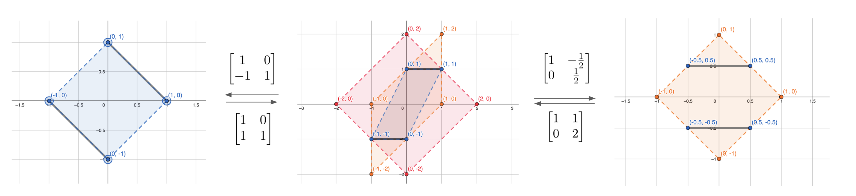
Figure 1: Comparison of Laplace mechanism tightest unit ball given different linear transformations. The middle figure shows the unit balls in the original 2D sensitivity space, where red=Algorithm 1; orange =Algorithm 2; blue=Algorithm 3, which is the smallest convex shape possible. The left figure shows the transformed space using the shifting in Algorithm 2; The right shows the transformed space using Algorithm 3.

Of course, the optimality of K-norm mechanism with the smallest convex hull is not guaranteed for any target metric. In the following sections, we show Algorithm 3 is in fact optimal for the mean squared error of the mean; and we get to release the count in add-remove model for free.

4 Analysis of algorithms

We first state a technical result which we use in proving the upper bound.

Lemma 1.

Let $b\geq 0$. Let $a$ be such that $|a|/b\leq M$. Let $C=\frac{Z_{a}}{b}-\frac{aZ_{b}}{b^{2}}$ and $F=\left\lvert\frac{2MZ^{2}_{b}}{b^{2}}\right\rvert+\left\lvert\frac{2Z_{a}Z_{b}}{b^{2}}\right\rvert$. Then,

$$\mathbb{E}\left[\left(\text{Clip}\left(\frac{a+Z_{a}}{b+Z_{b}}\right)-\frac{a}{b}\right)^{2}\right] \leq\mathbb{E}\left[C^{2}\right]+\mathbb{E}\left[F^{2}\right]+2\sqrt{\mathbb{E}\left[C^{2}\right]\mathbb{E}\left[F^{2}\right]}+4M^{2}\text{Pr}(Z_{b}<-b/2).$$

We provide the proof of the above result in the appendix. We now state the upper bound on the mean squared error of Algorithm 2.

Lemma 2.

The output of Algorithm 2 is $\varepsilon$-differentially private. For any dataset $D\in\mathcal{D}^{*}(\ell,u)$, the mean squared error of Algorithm 2 is

$$\mathbb{E}[(\hat{\mu}(D)-\mu(D))^{2}] \leq\left(\frac{2(u-l)^{2}}{|D|^{2}\varepsilon^{2}}+\frac{8(\mu-m)^{2}}{|D|^{2}\varepsilon^{2}}\right)\left(1+o(1)\right)$$

$$\leq\frac{4(u-l)^{2}}{|D|^{2}\varepsilon^{2}}\left(1+o(1)\right),$$

where $m=\frac{\ell+u}{2}$.

Proof.

The differential privacy guarantee follows by the properties of Laplace mechanism and composition theorem and in the rest of the proof, we focus on the MSE guarantees. The analysis of MSE heavily relies in Lemma 1. Let $n=|D|$, $a=s$, $b=n$, $Z_{a}=Z_{s}\sim\text{Lap}(w/\varepsilon)$, $Z_{b}=Z_{n}=\text{Lap}(2/\varepsilon)$, and $M=(u-\ell)/2$. With these definitions, to apply Lemma 1, we need to bound $\mathbb{E}[C^{2}]$, $\mathbb{E}[F^{2}]$, and $\text{Pr}(Z_{b}<-b/2)$. We bound each of the terms below.

$$\mathbb{E}[C^{2}]=\mathbb{E}\left[\left(\frac{Z_{s}}{n}-\frac{(\mu-m)Z_{n}}{n}\right)^{2}\right]=\frac{2(u-l)^{2}}{n^{2}\varepsilon^{2}}+\frac{8(\mu-m)^{2}}{n^{2}\varepsilon^{2}}.$$

Since $(x+y)^{2}\leq 2x^{2}+2y^{2}$,

$$\mathbb{E}[F^{2}]\leq 8\frac{(u-\ell)^{2}}{n^{4}}\mathbb{E}\left[Z^{4}_{n}\right]+8\frac{1}{n^{4}}\mathbb{E}\left[Z^{2}_{a}Z^{2}_{b}\right]=o\left(\frac{(u-l)^{2}}{n^{2}\varepsilon^{2}}\right).$$

Finally, by the tail bounds of the Laplace mechanism,

$$M^{2}\text{Pr}(Z_{b}<-b/2)\leq(u-\ell)^{2}\text{Pr}(Z_{n}<-n/2)=o\left(\frac{(u-l)^{2}}{n^{2}\varepsilon^{2}}\right).$$

Combining the above three equations together with Lemma 1 yields the lemma. ∎

We now prove the upper bound on the mean squared error of Algorithm 3.

Theorem 1.

The output of Algorithm 3 is $\varepsilon$-differentially private. Furthermore, for any dataset $D\in\mathcal{D}^{*}(\ell,u)$, the mean squared error of Algorithm 3 is

$$\mathbb{E}[(\hat{\mu}-\mu)^{2}] \leq\left(\frac{(u-l)^{2}}{|D|^{2}\varepsilon^{2}}+\frac{4(\mu-m)^{2}}{|D|^{2}\varepsilon^{2}}\right)\left(1+o(1)\right)$$

$$\leq\frac{2(u-l)^{2}}{|D|^{2}\varepsilon^{2}}\left(1+o(1)\right),$$

where $m=\frac{\ell+u}{2}$.

Proof.

Let $s=[s_{1},s_{2}]$. $s$ is a two-dimensional vector. Let $s^{\prime}$ and $s^{\prime\prime}$ are vectors corresponding to two neighboring datasets. Then, the $L_{1}$ sensitivity is bounded by

$$\|s^{\prime}-s^{\prime\prime}\|_{1}\leq w.$$

In lines $5$ and $6$ of the algorithm, we add $\text{Lap}(w/\varepsilon)$ noise to each coordinate. Hence $[\hat{s}_{1},\hat{s}_{2}]$ is an $\varepsilon$ differentially private vector and by the postprocessing lemma, the output $\hat{\mu}$ is $\varepsilon$ differentially private. Similar to the previous lemma, the proof heavily relies in Lemma 1. Let $n=|D|$. Observe that

$$\mathbb{E}[(\hat{\mu}-\mu)^{2}]=(u-\ell)^{2}\mathbb{E}\left[\left(\frac{\hat{s}_{1}}{\hat{s}_{1}+\hat{s}_{2}}-\frac{s_{1}}{n}\right)^{2}\right].$$

Let $a=s_{1}$, $b=n$, $Z_{a}=Z_{1}\sim\text{Lap}(1/\varepsilon)$, $Z_{b}=Z_{1}+Z_{2}$, and $M=1$. With these definitions, to apply Lemma 1, we need to bound $\mathbb{E}[C^{2}]$, $\mathbb{E}[F^{2}]$, and $\text{Pr}(Z_{b}<-b/2)$. We bound each of the terms below.

$$\mathbb{E}[C^{2}]=\mathbb{E}\left[\left(\frac{Z_{1}}{n}-\frac{(\frac{s_{1}}{n})(Z_{1}+Z_{2})}{n}\right)^{2}\right]=\frac{1}{n^{2}\varepsilon^{2}}+\frac{4(\frac{s_{1}}{n}-\frac{1}{2}))^{2}}{n^{2}\varepsilon^{2}}.$$

Since $(x+y)^{2}\leq 2x^{2}+2y^{2}$,

$$\mathbb{E}[F^{2}]\leq\frac{8}{n^{4}}\mathbb{E}[(Z_{1}+Z_{2})^{4}]+\frac{8}{n^{4}}\mathbb{E}[(Z_{1}+Z_{2})^{2}Z^{2}_{1}]=o\left(\frac{1}{n^{2}\varepsilon^{2}}\right).$$

Finally,

$$\text{Pr}(Z_{b}<-b/2)\leq\text{Pr}(Z_{1}+Z_{2}<-n/2)\leq\text{Pr}(Z_{1}<-n/4)+\text{Pr}(Z_{2}<-n/4)=o\left(\frac{1}{n^{2}\varepsilon^{2}}\right).$$

Combining the above three equations together with Lemma 1 and observing the fact that $\mu=\ell+\frac{s_{1}}{n}$ yields the theorem. ∎

The above theorem implies the following corollary.

Corollary 1.

$$R_{ar}(\varepsilon,\ell,u)\leq\frac{2(u-l)^{2}}{n^{2}\varepsilon^{2}}\left(1+o(1)\right).$$

5 Lower bound

We first state the following lemma, which removes the dependence on $\ell$ and $u$.

Lemma 3.

$$R_{ar}(\varepsilon,\ell,u)=(u-\ell)^{2}R_{ar}(\varepsilon,0,1).$$

Proof.

Given a dataset from $D\in\mathcal{D}^{*}(\ell,u)$, one can create a dataset in $f(D)\in\mathcal{D}^{*}(0,1)$ by applying the transformation $f(x)=\frac{x-\ell}{u-\ell}$ to each of the points. Let $\hat{\mu}$ be a mean estimation algorithm for datasets in $\mathcal{D}^{*}(0,1)$, then given a dataset from $D\in\mathcal{D}^{*}(\ell,u)$, one can scale all points by applying $f$ and compute the output as $\hat{\mu}^{\prime}(D)=f^{-1}(\hat{\mu}(f(D))$. If $\hat{\mu}$ is an $\varepsilon$-differentially private algorithm, then $\hat{\mu}^{\prime}$ is also an $\varepsilon$-differentially private algorithm. Furthermore, the utilities are related by

$$L(\hat{\mu}^{\prime},D)\leq(u-\ell)^{2}L(\hat{\mu},f(D)).$$

Taking supremum over datasets $D$ and infimum over all differentially private algorithms yields

$$R_{ar}(\varepsilon,\ell,u)\leq(u-\ell)^{2}R_{ar}(\varepsilon,0,1).$$

The proof for the other direction is similar and omitted. ∎

We now state a well known result from Geng and Viswanath (2014), that we will use to prove the bound.

Lemma 4 ( Geng and Viswanath (2014, Section VI.C) ).

Let $k>0$ and $n>0$. Let $D_{i}$ denote the dataset that contains $i$ values of $1$ and $n$ values of $0$. Let $\mathcal{D}^{k}=\{\mathcal{D}_{1},\mathcal{D}_{2},\ldots,\mathcal{D}_{k}\}$. Let $N(D_{i})$ denote the number of $1$s in $D_{i}$ and let $\hat{N}$ denote an estimator. Then for any $\varepsilon<\varepsilon_{0}\ll 1$,

$$\inf_{\hat{N}\in\mathcal{A}^{\text{ar}}_{\varepsilon}}\sup_{D\in\mathcal{D}^{k}}\mathbb{E}\left[(\hat{N}-N(D))^{2}\right]\geq\frac{2}{\varepsilon^{2}}(1-o(1)),$$

and the best way to get $\hat{N}$ is to noise $N(D_{i})$ with a geometric mechanism. Here $o(1)$ term goes to zero as $k$ tends to infinity and $\varepsilon$ goes to $0$.

Theorem 2.

$$R_{ar}(\varepsilon,\ell,u)\geq\frac{2(u-l)^{2}}{\varepsilon^{2}}\left(1-o(1)\right).$$

Proof.

By Lemma 3, it suffices to consider the scenario when $\ell=0$ and $R=1$. Let $\mathcal{D}^{k}$ and $N(D_{i})$ be the same as those be defined as in Lemma 4. Observe for any dataset $D$ in $\mathcal{D}^{k}$,

$$\mu(D)=\frac{N(D)}{n+N(D)}\leq\frac{k}{n}.$$

Suppose we have an $\varepsilon$-differentially private estimator $\hat{\mu}$ on $\mathcal{D}^{k}$. We convert it to an estimator of $N(D)$ as

$$\hat{N}=n\hat{\mu}(D).$$

For this estimator, based on the Lemma 4, there exists a $D\in\mathcal{D}^{k}$ such that

$$\mathbb{E}\left[(\hat{N}-N(D))^{2}\right]\geq\frac{2}{\varepsilon^{2}}(1-o(1))$$

and hence

$$\mathbb{E}\left[(n\hat{\mu}-N(D))^{2}\right]\geq\frac{2}{\varepsilon^{2}}(1-o(1))$$

We now upper bound the left hand side of the above expression.

$$\mathbb{E}\left[(n\hat{\mu}-N(D))^{2}\right] =\mathbb{E}\left[(n\hat{\mu}-n\mu+n\mu-N(D))^{2}\right]$$

$$=\mathbb{E}\left[(n\hat{\mu}-n\mu+n\mu-N(D))^{2}\right]$$

$$=\mathbb{E}\left[(n\hat{\mu}-n\mu-\mu(D)N(D))^{2}\right]$$

$$=\mathbb{E}\left[(n\hat{\mu}-n\mu)^{2}\right]+\mathbb{E}\left[(\mu(D)N(D))^{2}\right]-2\mathbb{E}\left[(n\hat{\mu}-n\mu)(\mu(D)N(D))\right]$$

$$\leq\mathbb{E}\left[(n\hat{\mu}-n\mu)^{2}\right]+\frac{k^{4}}{n^{2}}+2\sqrt{\mathbb{E}\left[(n\hat{\mu}-n\mu)^{2}\right]}\frac{k^{2}}{n}$$

$$\leq\mathbb{E}\left[(n\hat{\mu}-n\mu)^{2}\right]+\frac{k^{4}}{n^{2}}+\frac{k^{3}}{n}$$

$$\leq|D|^{2}\mathbb{E}\left[(\hat{\mu}-\mu)^{2}\right]+\frac{k^{4}}{n^{2}}+\frac{k^{3}}{n},$$

where the first inequality follows by Cauchy-Schwarz inequality and the second inequality follows by observing that both $\hat{\mu}$ and $\mu$ lie in $[0,k/n]$. Setting $k=o(n^{1/3}/\varepsilon^{1/3})$ yields the following theorem. ∎

6 Experiments

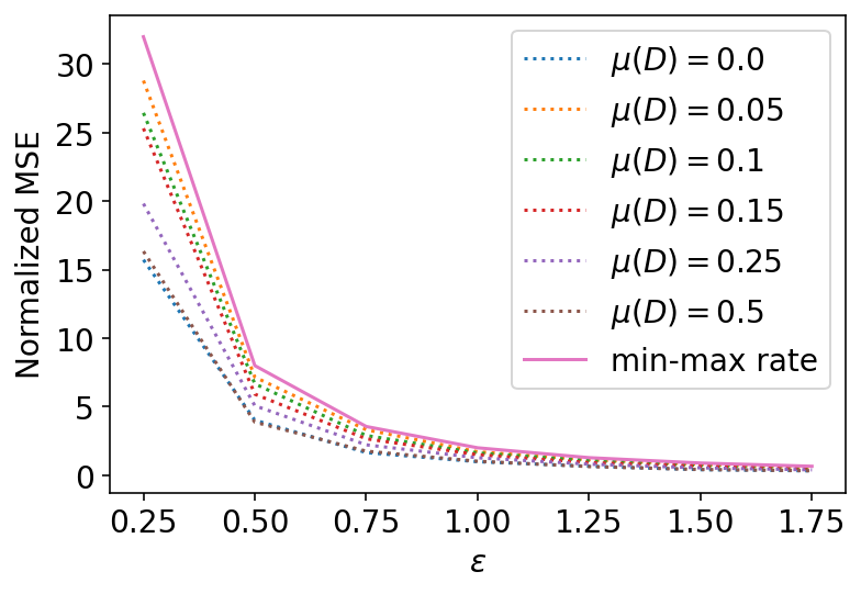
(a) Normalized MSE of Algorithm 3.

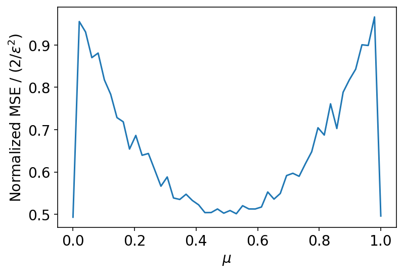
(b) Ratio of Normalized MSE of Algorithm 3 to the theoretical bound for $\varepsilon=0.5$.

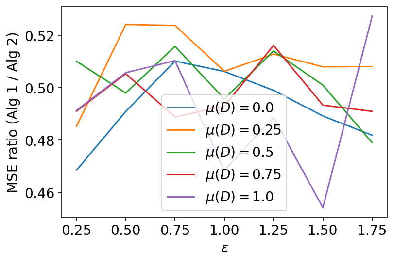
(c) Ratio of mean squared errors of Algorithm 3 and Algorithm 2.

Figure 2: All experiments are conducted over datasets of size $1,000$ and experiments are repeated $10,000$ times for statistical consistency.

Without loss of generality, we set $\ell=0$ and $u=1$ throughout the experiments. All datasets have $1,000$ points and the experiments are repeated $10,000$ times for statistical consistency. In Figure 2(a), we plot the performance of Algorithm 3 for different values of $\varepsilon$ and for different values of true mean. Observe that the experiments validate theory. To further verify the difficult cases for the proposed algorithm, we fix $\varepsilon=0.5$ and vary $\mu$ and plot the ratio of normalized MSE to the theoretical bound of $2/\varepsilon^{2}$ in Figure 2(b). Observe that as the theory predicts, the ratio is highest when $\mu=\Theta(1/n\varepsilon)$.

Finally, we plot the performance ratio of MSE of Algorithms 2 and 3 for various values of $\varepsilon$ and for different values of true mean in Figure 2(c). Observe that the factor is roughly around two.

7 Acknowledgements

The authors thank Travis Dick and Ziteng Sun for helpful comments and suggestions.

Appendix A Proof of Lemma 1

We first focus on the upper bound.

$$\left(\text{Clip}\left(\frac{a+Z_{a}}{b+Z_{b}}\right)-\frac{a}{b}\right)^{2} =\left(\text{Clip}\left(\frac{a+Z_{a}}{b+Z_{b}}\right)-\frac{a}{b}\right)^{2}1_{Z_{b}\geq-b/2}+\left(\text{Clip}\left(\frac{a+Z_{a}}{b+Z_{b}}\right)-\frac{a}{b}\right)^{2}1_{Z_{b}<-b/2}$$

$$\leq\left(\text{Clip}\left(\frac{a+Z_{a}}{b+Z_{b}}\right)-\frac{a}{b}\right)^{2}1_{Z_{b}\geq-b/2}+4M^{2}1_{Z_{b}<-b/2}$$

$$\leq\left(\text{Clip}\left(\frac{a+Z_{a}}{b+Z_{b}}\right)-\frac{a}{b}\right)^{2}1_{Z_{b}\geq-b/2}+4M^{2}1_{Z_{b}<-b/2},$$

where the first inequality uses the fact that both $\text{Clip}\left(\frac{a+Z_{a}}{b+Z_{b}}\right)$ and $\frac{a}{b}$ lie in $[0,1]$ and the last inequality uses the fact that clipping is a projection operator. Taking expectation on both sides yield,

$$\mathbb{E}\left[\left(\text{Clip}\left(\frac{a+Z_{a}}{b+Z_{b}}\right)-\frac{a}{b}\right)^{2}\right] \leq\mathbb{E}\left[\left(\frac{a+Z_{a}}{b+Z_{b}}-\frac{a}{b}\right)^{2}1_{Z_{b}\geq-b/2}\right]+4M^{2}\text{Pr}(Z_{b}<-b/2).$$

We now use algebraic manipulation to simplify $\frac{a+Z_{a}}{b+Z_{b}}-\frac{a}{b}$.

$$\frac{a+Z_{a}}{b+Z_{b}}-\frac{a}{b} =\frac{Z_{a}}{b}+\frac{a+Z_{a}}{b+Z_{b}}-\frac{a+Z_{a}}{b}$$

$$=\frac{Z_{a}}{b}-\frac{(a+Z_{a})(Z_{b})}{(b+Z_{b})(b)}$$

$$=\frac{Z_{a}}{b}-\frac{aZ_{b}}{(b+Z_{b})(b)}-\frac{Z_{a}Z_{b}}{(b+Z_{b})(b)}$$

$$=\frac{Z_{a}}{b}-\frac{aZ_{b}}{b^{2}}+\frac{aZ_{b}}{b^{2}}-\frac{aZ_{b}}{(b+Z_{b})(b)}-\frac{Z_{a}Z_{b}}{(b+Z_{b})(b)}$$

$$=\frac{Z_{a}}{b}-\frac{aZ_{b}}{b^{2}}+\frac{aZ^{2}_{b}}{b^{2}(b+Z_{b})}-\frac{Z_{a}Z_{b}}{(b+Z_{b})(b)}.$$

Let $C=\frac{Z_{a}}{b}-\frac{aZ_{b}}{b^{2}}$ and $D=\frac{aZ^{2}_{b}}{b^{2}(b+Z_{b})}-\frac{Z_{a}Z_{b}}{(b+Z_{b})(b)}$.

$$\mathbb{E}\left[\left(\frac{a+Z_{a}}{b+Z_{b}}-\frac{a}{b}\right)^{2}1_{Z_{b}\geq-b/2}\right] =\mathbb{E}\left[\left(C+D\right)^{2}1_{Z_{b}\geq-b/2}\right]$$

$$=\mathbb{E}\left[C^{2}1_{Z_{b}\geq-b/2}\right]+\mathbb{E}\left[D^{2}1_{Z_{b}\geq-b/2}\right]+\mathbb{E}\left[2CD1_{Z_{b}\geq-b/2}\right]$$

$$\leq\mathbb{E}\left[C^{2}1_{Z_{b}\geq-b/2}\right]+\mathbb{E}\left[D^{2}1_{Z_{b}\geq-b/2}\right]+2\sqrt{\mathbb{E}\left[C^{2}\right]\mathbb{E}\left[D^{2}1_{Z_{b}\geq-b/2}\right]},$$

where the last inequality uses Cauchy-Schwarz inequality. We next upper bound $D$. If $Z_{b}\geq-b/2$, and $|a|\leq bM$, then

$$|D|=\left\lvert\frac{aZ^{2}_{b}}{b^{2}(b+Z_{b})}-\frac{Z_{a}Z_{b}}{(b+Z_{b})(b)}\right\rvert \leq\left\lvert\frac{aZ^{2}_{b}}{b^{2}(b+Z_{b})}\right\rvert+\left\lvert\frac{Z_{a}Z_{b}}{(b+Z_{b})(b)}\right\rvert$$

$$\leq\left\lvert\frac{MZ^{2}_{b}}{b(b+Z_{b})}\right\rvert+\left\lvert\frac{Z_{a}Z_{b}}{(b+Z_{b})(b)}\right\rvert$$

$$\leq\left\lvert\frac{2MZ^{2}_{b}}{b^{2}}\right\rvert+\left\lvert\frac{2Z_{a}Z_{b}}{b^{2}}\right\rvert.$$

Let $F=\left\lvert\frac{2MZ^{2}_{b}}{b^{2}}\right\rvert+\left\lvert\frac{2Z_{a}Z_{b}}{b^{2}}\right\rvert$. Combing the above bound with previous equations yields the upper bound:

$$\mathbb{E}\left[\left(\frac{a+Z_{a}}{b+Z_{b}}-\frac{a}{b}\right)^{2}1_{Z_{b}\geq-b/2}\right] \leq\mathbb{E}\left[C^{2}1_{Z_{b}\geq-b/2}\right]+\mathbb{E}\left[D^{2}1_{Z_{b}\geq-b/2}\right]+2\sqrt{\mathbb{E}\left[C^{2}\right]\mathbb{E}\left[D^{2}1_{Z_{b}\geq-b/2}\right]}$$

$$\leq\mathbb{E}\left[C^{2}1_{Z_{b}\geq-b/2}\right]+\mathbb{E}\left[F^{2}1_{Z_{b}\geq-b/2}\right]+2\sqrt{\mathbb{E}\left[C^{2}\right]\mathbb{E}\left[F^{2}1_{Z_{b}\geq-b/2}\right]}$$

$$\leq\mathbb{E}\left[C^{2}\right]+\mathbb{E}\left[F^{2}\right]+2\sqrt{\mathbb{E}\left[C^{2}\right]\mathbb{E}\left[F^{2}\right]}.$$

References

- Amin et al. [2019] K. Amin, A. Kulesza, A. Munoz, and S. Vassilvtiskii. Bounding user contributions: A bias-variance trade-off in differential privacy. In International Conference on Machine Learning, pages 263–271. PMLR, 2019.
- Amin et al. [2022] K. Amin, J. Gillenwater, M. Joseph, A. Kulesza, and S. Vassilvitskii. Plume: differential privacy at scale. arXiv preprint arXiv:2201.11603, 2022.
- Dick et al. [2023] T. Dick, A. Kulesza, Z. Sun, and A. T. Suresh. Subset-based instance optimality in private estimation. arXiv preprint arXiv:2303.01262, 2023.
- Dwork et al. [2006] C. Dwork, F. McSherry, K. Nissim, and A. Smith. Calibrating noise to sensitivity in private data analysis. In Theory of Cryptography: Third Theory of Cryptography Conference, TCC 2006, New York, NY, USA, March 4-7, 2006. Proceedings 3, pages 265–284. Springer, 2006.
- Dwork et al. [2014] C. Dwork, A. Roth, et al. The algorithmic foundations of differential privacy. Foundations and Trends® in Theoretical Computer Science, 9(3–4):211–407, 2014.