Learning Naturally Aggregated Appearance for Efficient 3D Editing

Abstract

Neural radiance fields, which represent a 3D scene as a color field and a density field, have demonstrated great progress in novel view synthesis yet are unfavorable for editing due to the implicitness. In view of such a deficiency, we propose to replace the color field with an explicit 2D appearance aggregation, also called canonical image, with which users can easily customize their 3D editing via 2D image processing. To avoid the distortion effect and facilitate convenient editing, we complement the canonical image with a projection field that maps 3D points onto 2D pixels for texture lookup. This field is carefully initialized with a pseudo canonical camera model and optimized with offset regularity to ensure naturalness of the aggregated appearance. Extensive experimental results on three datasets suggest that our representation, dubbed AGAP, well supports various ways of 3D editing (e.g., stylization, interactive drawing, and content extraction) with no need of re-optimization for each case, demonstrating its generalizability and efficiency. Project page is available at https://felixcheng97.github.io/AGAP/.

1 Introduction

While recent advancements in 3D representations like neural radiance fields (NeRF) [31] have shown impressive reconstruction capabilities for real-world scenes, the need for further progress in 3D editing arises as the desire to recreate and manipulate these scenes. The field of 3D editing has witnessed significant development in recent years. Traditional 3D modeling approaches [21, 43, 42, 55] typically rely on reconstructing scenes using meshes. By combining meshes with texture maps, we can enable appearance editing during the rendering process. However, these methods usually face difficulties in obtaining detailed and regular texture maps, typically in complex scenes, which significantly hinders effective editing and compromises user-friendliness.

Recent neural radiance fields offer high-quality scene reconstruction capabilities, but manipulating the implicit 3D representation embedded within neural networks is inherently complex and non-straightforward. Existing NeRF-based editing approaches can be mainly divided into two categories: some methods like [8, 9, 52, 56, 59, 63] target geometry editing, usually taking advantage of meshes, while the other [14, 36, 24, 60, 62] focuses on 3D stylization using images or texts as style guidance. However, re-optimizing the pre-trained NeRF models is necessary to incorporate the desired editing effects into the underlying 3D representation, resulting in time-consuming processes. Consequently, it is crucial to develop a user-friendly framework that can efficiently and effectively support various edits within a single model.

In this paper, we introduce a novel editing-friendly representation AGAP with naturally Aggregated Appearance, consisting of a 3D density grid for geometry estimation and a canonical image plus a projection field for appearance or texture modeling. Our method attempts to link the 3D representation with a natural 2D aggregated canonical representation. Concretely, a learnable canonical image is designed as the interface for editing, which aggregates the appearance by projecting the 3D radiance to a natural-looking image by the associated projection field. To ensure the naturalness of the aggregated canonical image with strong representation capacity, the associated projection field is carefully initialized by a pseudo canonical camera model and complemented by a learned view-dependent offset. The underlying 3D structure is modeled by an explicit 3D density grid. After a scene is optimized through volume rendering, AGAP supports various ways of 3D editing in a user-friendly setting by applying different 2D image processing tools on the canonical images without re-optimization of the original model. We evaluate the effectiveness of our method on three datasets, including LLFF [30], Replica [46, 13], and Instruct-NeRF2NeRF [14] in various editing tasks, which are scene stylization, content extraction, and texture editing (i.e., drawing). Experimental results further show that AGAP can achieve on-par performance with NeRF [31] in terms of PSNR with a hash grid-based projection field.

2 Related Work

Implicit 3D representation. 3D modeling [1, 17, 19, 45, 50, 51, 27, 15] is pivotal in computer graphics and computer vision. Traditionally, explicit representations such as voxels and meshes have been employed for 3D shape modeling, but they often face challenges related to detail preservation and limited flexibility in processing. In contrast, implicit 3D representation like NeRF [31], SDF [37, 52, 57], Occupancy Networks [29], describing 3D scenes through continuous implicit functions, excels in capturing detailed geometry with improved fidelity. Many further works aim at improving NeRF in terms of various aspects, such as modeling capacity [3, 2], generative modeling [53, 44, 6, 12], and camera pose estimation [26, 54, 25]. In particular, methods like DVGO [47], Plenoxels [11], InstantNGP [32], TensoRF [7] focus on improving the convergence speed of volume rendering for 3D scenes by modeling the geometry and appearance with explicit grid representations. Our method leverages this technique for our density grid and canonical image as well, enabling efficient and rapid convergence of 3D modeling.

Neural scene editing. Existing research on NeRF editing can be broadly categorized into two: one focuses on editing the geometry [8, 9, 52, 56, 59, 63]; the other, known as style-based editing [14, 36, 24, 60, 62], aims to achieve scene stylization. Our research aligns with the latter category. Many NeRF stylization methods [60, 16, 33] have adopted techniques from 2D image stylization with style loss and content loss on images for NeRF optimization. While these methods can deliver 3D-consistent editing, they are primarily limited to global texture modifications and lack flexibility. Later, CLIP-NeRF [49] incorporates text conditions by regularizing the CLIP embeddings of the global scene with input prompts. Subsequent studies [24] extract 2D features such as DINO [5, 34] for local editing. Most recently, Instruct-Nerf2Nerf [14] proposes an iterative approach to edit the input images using pre-trained diffusion models [4] for underlying NeRF optimization. Despite achieving high-fidelity editing results, these methods necessitate optimization for each text prompt or reference image, which is inefficient.

Neural atlases. Our work shares similar insights with the research area of neural atlases [20, 58, 35], which decompose videos into a canonical form with learned deformations, thereby enabling consistent video editing. Approaches such as neural layered atlases [20] employ an implicit network to distinguish foreground and background movement, dividing them into distinct layers. The CoDeF [35] methodology represents 2D videos using content deformation fields by integrating 3D hash tables [32]. However, these approaches lack 3D priors, limiting the effectiveness of 3D viewpoint changes in 3D scene editing.

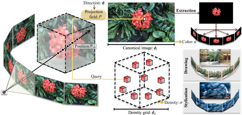
Figure 2: The overall pipeline. AGAP consists of two components: (1) an explicit 3D density grid $\phi_{G}$ to estimate geometry for density $\sigma$; (2) an explicit canonical image $\phi_{I}$ with an associated view-dependent projection field $P$ to aggregate appearance for color $\mathbf{c}$. By performing 2D image processing on the canonical image, our method enables various editing (e.g., content extraction, interactive drawing, and scene stylization) through volume rendering without the need for re-optimization.

3 Method

Formally, given a set of multi-view training images $\mathcal{I}$, our method models the scene appearance by an explicit canonical image $\phi_{I}$ plus a corresponding implicit projection field $P$ inspired by [35, 39, 38]; the scene geometry is estimated by an explicit 3D density grid $\phi_{G}$. With such a representation, one can render different views of the scene through volume rendering. Our key property is that by explicitly editing the canonical image $\phi_{I}$, it can propagate the edited appearance to the whole scene through the projection field $P$ without any further re-optimization. An overview of our framework is shown in Fig. 2.

3.1 Preliminary

Volume rendering [18, 31] accumulates colors and densities of the 3D points sampled along the camera rays to render images. For a given camera ray $\mathbf{r}(t)=\mathbf{o}+t\mathbf{d}$ denoted by its origin $\mathbf{o}\in\mathbb{R}^{3}$ and direction $\mathbf{d}\in\mathbb{R}^{3}$, we sample $N$ points $\{\mathbf{r}(t_{i})\}_{i=1}^{N}$ along the ray defined by a sorted distance vector $\mathbf{t}=[t_{1},...,t_{N}]^{T}\in\mathbb{R}^{N}$.

NeRF [31] models the 3D scene implicitly and leverage MLP networks to decode the density $\sigma_{i}=\mathtt{MLP}(\mathbf{r}(t_{i}))$ and the view-dependent color $\mathbf{c}_{i}=\mathtt{MLP}(\mathbf{r}(t_{i}),\mathbf{d})$ of a point located at $\mathbf{r}(t_{i})$ on the ray with viewing direction $\mathbf{d}$. To render the image pixel $\hat{C}(\mathbf{r})$, we apply discretized volume rendering by Max [28] along the $N$ sampled ray points with $\delta_{i}$ denoting the distance to the nearby sampled points:

$$\begin{split}\hat{C}(\mathbf{r})&=\sum_{i=1}^{N}{T_{i}(1-\exp(-\sigma_{i}\delta_{i}))\mathbf{c}_{i}},\text{where}\\ T_{i}&=\exp(-\sum_{j=1}^{i-1}{\sigma_{j}\delta_{j}}).\end{split}$$ (1)

Training such MLPs for 3D radiance field modeling requires observed images with known camera poses. Specifically, NeRF model is optimized by minimizing the average $\mathcal{L}_{2}$ distance between the rendered pixel color $\hat{C}(\mathbf{r})$ and the ground-truth pixel color $C(\mathbf{r})$:

$$\mathcal{L}_{color}=\frac{1}{|\mathcal{R}|}\sum_{\mathbf{r}\in\mathcal{R}}{\left\|\hat{C}(\mathbf{r})-C(\mathbf{r})\right\|_{2}^{2}}.$$ (2)

3.2 Model Formulation

Our representation disentangles the density and color of the scene and uses different modalities for modeling.

Density. Similar to DVGO [47], we adopt a voxel-grid representation to model the 3D density for an efficient query. Given a particular query point $\mathbf{p}_{xyz}\triangleq\mathbf{r}(t_{i})\in\mathbb{R}^{3}$, we can obtain the corresponding density $\sigma\in\mathbb{R}$ via a trilinear interpolation, followed by a Softplus activation:

$$\sigma=\mathtt{Softplus}(\mathtt{GridSample}(\mathbf{p}_{xyz},\phi_{G})),$$ (3)

where $\phi_{G}$ denotes the one-channel voxel grid with learnable parameter $\phi_{g}$ at a voxel resolution size of $N_{x}\times N_{y}\times N_{z}$. Concerning the fact that in 3D reconstruction, textures are applied to the surface of the mesh to provide visual details such as colors, patterns, and material properties [51, 17], we hope our model can obtain a coarsely accurate density estimation to perceive the 3D geometry at the early training stage, facilitating the subsequent learning of appearance aggregation. Hence, we opt for an explicit voxel-grid representation to achieve fast convergence instead of utilizing an implicit MLP such as NeRF [31]. Such a choice is also proven to be crucial by our experiments in Sec. 4.4.

Appearance. In order to empower explicit 3D editing capabilities, we formulate the color appearance by an explicit canonical image $\phi_{I}\in\mathbb{R}^{H\times W\times 3}$ plus an associated view-dependent implicit projection field $P(\cdot,\cdot):(\mathbb{R}^{3},\mathbb{R}^{3})\to\mathbb{R}^{2}$, where $H$ and $W$ represent the image height and width, respectively. This formulation maps a given query point $\mathbf{p}_{xyz}$ in the 3D field with viewing direction $\mathbf{d}$ to the projected 2D point $\mathbf{p}_{uv}$ on the canonical image $\phi_{I}$.

The design of the projection field is crucial to achieving naturalness and completeness in the learned canonical image. We model the projection field $P$ in a residual manner, which consists of a non-learnable canonical projection initialization $P_{c}$ and a projection offset learning $P_{o}$. The canonical projection initialization $P_{c}$ plays a significant role in ensuring a natural-looking canonical image, while the projection offset $P_{o}$ aims to address view-dependent effects and handle occlusions present in complex scenes.

Specifically, the canonical projection initialization $P_{c}(\cdot):\mathbb{R}^{3}\to\mathbb{R}^{2}$ projects the query 3D point $\mathbf{p}_{xyz},$ to an initial 2D projection point $\tilde{\mathbf{p}}_{uv}$ on the canonical image. Further elaboration on the selection of an appropriate projection initializing function $P_{c}$ will be provided in Sec. 3.3. The projection offset $\Delta\mathbf{p}_{uv}$ is modeled by $P_{o}$ with parameter weights $\phi_{P}$:

$$\Delta\mathbf{p}_{uv}=P_{o}(\mathbf{p}_{xyz},\mathbf{d};\phi_{P}).$$ (4)

For simplicity, we omit the 3D positional encoding $\gamma_{p}$ of $\mathbf{p}_{xyz}$ and the viewing direction encoding $\gamma_{d}$ of $\mathbf{d}$ in Eq. 4. The final projection point $\mathbf{p}_{uv}$ can be derived as follows:

$$\mathbf{p}_{uv}=\tilde{\mathbf{p}}_{uv}+\Delta\mathbf{p}_{uv}=P_{c}(\mathbf{p}_{xyz})+P_{o}(\mathbf{p}_{xyz},\mathbf{d};\phi_{P}).$$ (5)

The projection point $\mathbf{p}_{uv}$ is then used to query the RGB color $\mathbf{c}\in\mathbb{R}^{3}$ from the canonical image $\phi_{I}$ via interpolation:

$$\mathbf{c}=\mathtt{Sigmoid}(\mathtt{GridSample}(\mathbf{p}_{uv},\phi_{I})).$$ (6)

3.3 Canonical Projection Initialization

Learning a good projection field $P$ for 3D-to-2D projection is indeed a non-trivial research challenge [10], particularly for 360-degree inward-facing scenes [3, 31]. Thus, we relax the 3D scene of interest in our approach, focusing on forward-facing scenes [30] and outward-facing panorama data [13]. The crucial step in achieving a natural-looking canonical image as the aggregated appearance is to position a pseudo canonical camera into the scene for a careful canonical projection initialization as $P_{c}$.

Forward-facing data and NDC representation. Similar to NeRF, we utilize the normalized device coordinate (NDC) space to model the real forward-facing captures. In perspective projection, the 3D points in the truncated pyramid frustum in camera (eye) coordinates are mapped to a cube $[-1,1]^{3}$ in NDC space. The pseudo canonical camera is defined as the average camera pose positioned at the world origin. By doing so, the perspective projection $f_{p}$ can map any given point $\mathbf{p}_{xyz}$ in the world coordinates to its corresponding NDC point $(p_{x^{\prime}},p_{y^{\prime}},p_{z^{\prime}})\triangleq f_{p}(\mathbf{p}_{xyz})$. The coordinate range of the voxel grid $\phi_{G}$ is defined by the bounding box in NDC space. Please refer to the original NeRF paper [31] for the detailed derivation of NDC.

One notable property of NDC is that for a ray $\mathbf{r}$ origin from the camera center, the resulting projected camera ray $\mathbf{r}^{\prime}$ in NDC space is always perpendicular to the $x^{\prime}y^{\prime}$ plane. This implies that all points along $\mathbf{r}^{\prime}$ share identical values for $p_{x^{\prime}}$ and $p_{y^{\prime}}$. Leveraging this property, we can have a simple and appropriate initialization for the projection field:

$$\tilde{p}_{u}=p_{x^{\prime}},\quad\tilde{p}_{v}=p_{y^{\prime}},$$ (7)

where we have the notation $(\tilde{p}_{u},\tilde{p}_{v})\triangleq\tilde{\mathbf{p}}_{uv}$.

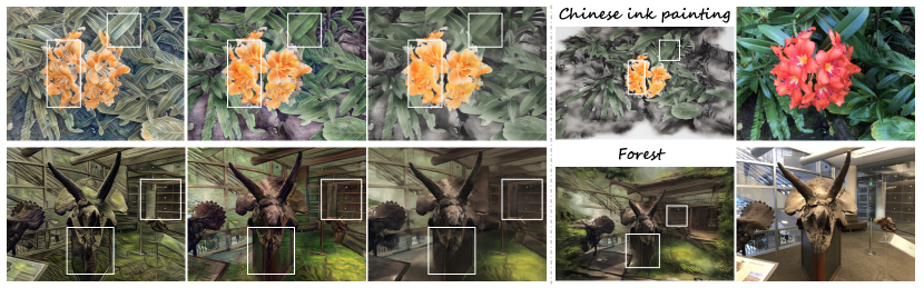
ARF [60]

Ref-NPR [62]

Ours

Stylized Reference

Reference View

Figure 3: Visual comparison of novel-view stylization results on the LLFF dataset given different reference images. Our method can better preserve textural consistencies as highlighted in the figure.

Panorama data and contracted representation. The training images for panorama scenes are typically captured by cameras positioned around the global origin, with outward-facing views covering a 360-degree field of view. We choose to place the pseudo canonical camera at the global origin and define the Equirectangular projected image as a feasible canonical projection initialization.

Drawing inspiration from the smooth coordinate transforms in [3, 40] for 360-degree inward-facing unbounded data, we introduce a new contracted formulation $f_{c}$ specifically for outward-facing (unbounded) panorama scenes:

$$f_{c}(\mathbf{x})=\frac{\mathbf{x}}{\left\|\mathbf{x}\right\|}(1-\frac{1}{\left\|\mathbf{x}\right\|+1}),$$ (8)

where $\mathbf{x}\in\mathbb{R}^{3}$ is a 3D point in Euclidean space. This design transforms the points in such a way that they are distributed proportionally to the disparity in a unit sphere. Accordingly, the voxel grid $\phi_{G}$ is a cube with range $[-1,1]^{3}$.

Using the contracted representation in Eq. 8, we have $(p_{x^{\prime}},p_{y^{\prime}},p_{z^{\prime}})\triangleq f_{c}(\mathbf{p}_{xyz})$. The canonical projection initialization $P_{c}$ from $\mathbf{p}_{xyz}$ in 3D space to the 2D canonical image pixel $(\tilde{p}_{u},\tilde{p}_{v})\triangleq\tilde{\mathbf{p}}_{uv}$ can be formulated as follows:

$$\tilde{p}_{u} =\tan^{-1}(\frac{p_{y^{\prime}}}{p_{x^{\prime}}}) \in[-\pi,\pi],$$ (9)

$$\tilde{p}_{v} =\sin^{-1}(p_{z^{\prime}}) \in[-\frac{\pi}{2},\frac{\pi}{2}].$$

3.4 Design and Regularization

Positional and hash encoding. The projection offset in  Eq. 4 employs Fourier positional encoding or multi-resolution hash encoding to capture high-frequency information. For $\gamma_{d}$, we specifically employ positional encoding [48]; as for $\gamma_{p}$, we choose either positional encoding or hash encoding [32]. The positional encoding is defined as $\gamma_{pe}(\cdot):\mathbb{R}^{3}\to\mathbb{R}^{3\times(1+2K)}$ to encode 3-dimensional vector $\mathbf{x}$ up to $K$ frequencies as $\gamma_{pe}(\mathbf{x})=[\mathbf{x},F_{1}(\mathbf{x}),...,F_{K}(\mathbf{x})]$, where $F_{k}(\mathbf{x})=[\sin(2^{k}\mathbf{x}),\cos(2^{k}\mathbf{x})]$; for hash encoding, we have $\gamma_{h}(\cdot):\mathbb{R}^{3}\to\mathbb{R}^{3+DK}$ to encode the vector $\mathbf{x}$ by a $K$-resolution hash grid with $D$-dimensional feature per layer as $\gamma_{h}(\mathbf{x})=[\mathbf{x},H_{1}(\mathbf{x}),...,H_{K}(\mathbf{x})]$, where $H_{k}(\mathbf{x})$ is a $D$-dimensional feature vector interpolated by $\mathbf{x}$ at the $k$-th resolution.

Anneal encoding. Motivated by Nerfies [38], the positional or hash encoding can incorporate an optional annealing learning strategy. To achieve this, we introduce a weight factor $w^{n}_{k}=\frac{1}{2}(1-\cos(\alpha^{n}_{k}\pi))$ for some encoded frequency $F_{k}^{n}$ or $H_{k}^{n}$ at some training step $n$, such that we have $F_{k}^{n}(\cdot)=w^{n}_{k}F_{k}(\cdot)$ and

$$\alpha^{n}_{k}=\min(\max(\frac{n-N_{s}}{N_{e}-N_{s}}K-k,0.0),1.0),$$ (10)

where $N_{s}$ and $N_{e}$ denote the start and end steps for anneal encoding, respectively. The strategy aims to facilitate the learning of low-frequency details and gradually incorporate high-frequency bands as the training progresses.

Progressive training. Similar to [3, 31, 47], we apply progressive scaling for our voxel grid $\phi_{G}$ and canonical image $\phi_{I}$ for a coarse-to-fine learning process. At specific scaling-up milestone steps, we increase the $\phi_{G}$ voxel count by a factor of 2 and the $\phi_{I}$ pixel count by a factor of 4.

Projection regularization. In order to obtain a visually natural canonical image $\phi_{I}$, one important regularization is to avoid the deviation from the perception by the defined pseudo canonical camera. We find the following simple regularization works well and stabilizes the training:

$$\mathcal{L}_{uv}=\left\|\Delta\mathbf{p}_{uv}\right\|_{2}^{2}.$$ (11)

Total variation regularization. To mitigate floating densities, we incorporate total variation regularization [41] $\mathcal{L}_{tv}$ into the density grid $\phi_{G}$. This regularization term is particularly beneficial during the initial stages of training.

Optimization objective. The final optimization process of our method to model the scene for efficient editing can be formulated as follows:

$$\phi_{G}^{*},\phi_{I}^{*},\phi_{P}^{*}=\operatorname*{arg\,min}_{\phi_{G},\phi_{I},\phi_{P}}{\mathcal{L}_{color}+\mathcal{L}_{uv}+\mathcal{L}_{tv}}.$$ (12)

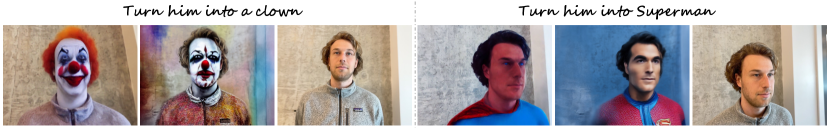
Haque et al. [14]

Ours

Reference Image

Haque et al. [14]

Ours

Reference Image

Figure 4: Visual comparison of scene stylization results on the Instruct-NeRF2NeRF dataset given different text prompts.

Novel Views  Canonical Image

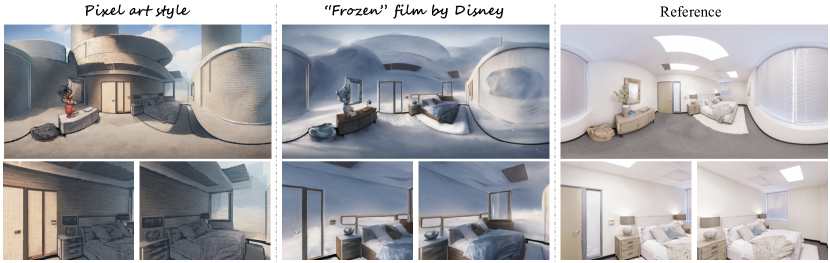
Figure 5: More visualization of scene stylization results on the panorama Replica dataset given different text prompts.

Foreground

Background

DFFs [24]

Ours

Reference

Figure 6: Visual comparison of foreground and background extraction results on the LLFF dataset.

(a) Multi-Object Extraction

(b) Custom Object Extraction

(c) Complex Object Extraction

(d) Extraction + Stylization

Figure 8: More visualization of content extraction results in different complex settings on the LLFF dataset.

Edited Novel View 1

Edited Novel View 2

Edited Novel View 3

Reference

Figure 10: Visualization of texture editing (i.e., drawing) results rendered at different novel viewpoints on the LLFF dataset.

4 Experiments

4.1 Experimental Setup

Datasets. The LLFF [30] dataset comprises 8 real-world scenes, where each scene is accompanied by several training images captured by handheld cameras placed in a rough grid pattern. We evaluate this dataset at a resolution of $1008\times 756$ after downscaling the images by a factor of 4.

The Replica [46] dataset is a collection of various high-quality and high-resolution 3D reconstructions of indoor scenes with clean and dense geometry. We evaluate the 14 panorama scenes as processed in SOMSI [13], where each scene is rendered as a grid of equally spaced spherical images at a resolution of $1024\times 512$.

The Instruct-NeRF2NeRF [14] dataset consists of 6 scenes captured in either an object-centric or forward-facing manner. We leverage this dataset specifically to model and edit forward-facing scenes that prominently feature human subjects for qualitative evaluation.

Implementation details. Our 3D editing pipeline involves a two-step process: training a per-scene reconstruction model and subsequent explicit edits on the canonical image $\phi_{I}$ for 3D scene editing. By default, we optimize a per-scene model for $60$k steps using the Adam optimizer [22] with an initial learning rate of $0.1$ for both the explicit 3D density grid $\phi_{G}$ and 2D canonical image $\phi_{I}$, and a learning rate of $0.001$ for the implicit projection field $P$ with learnable parameter $\phi_{P}$. All experiments are conducted and tested on a single RTX A6000 GPU. For further details and hyperparameters used in training different models, please refer to the supplementary materials.

Table 1: The reconstruction results on the LLFF dataset in terms of PSNR. Our PE-based models, which exhibit superior editing capacity, demonstrate satisfactory performance, while our hash-based models achieve reconstruction comparable to NeRF [31] and DVGO [47].

rowsep=1.2pt colsep=9.5pt Room Fern Leaves Fortress Orchids Flowers T-Res Horns Average LLFF [30] 28.42 22.85 18.52 29.40 18.52 25.46 24.15 24.70 24.13 NeRF [31] 32.70 25.17 20.92 31.16 20.36 27.40 26.80 27.45 26.50 DVGO [47] 31.43 25.08 21.03 30.47 20.37 27.59 27.17 27.56 26.34 Ours (PE) 30.22 22.77 19.96 29.15 18.39 26.38 25.85 25.97 24.83 Ours (Hash) 32.10 24.13 20.64 30.12 20.10 27.47 27.24 27.81 26.20

Table 2: The reconstruction results on the Replica dataset.

rowsep=1.2pt colsep=6.2pt PSNR $\uparrow$ SSIM $\uparrow$ SOMSI [13] 39.54 0.986 Ours (PE) 38.42 0.979 Ours (Hash) 38.68 0.976

4.2 Evaluation on Editability

By performing explicit edits on the canonical image $\phi_{I}$, our model is capable of propagating the editing effects through the learned projection field $P$. This enables various 3D scene editing functionalities, such as scene stylization, context extraction, and texture editing. Specifically, except for explicit texture editing, we leverage several state-of-the-art models for 2D image editing. Specifically, we utilize the prompt-guided ControlNet [61] for scene stylization and Segment-anything (SAM) [23] for content extraction.

Scene stylization. We conduct a comparative analysis between our method and three state-of-the-art stylization methods: ARF [60], Ref-NPR [62], and Instruct-NeRF2NeRF [14]. All three baseline methods require additional optimization processes to achieve stylization with a specific style, somehow limiting their model practicability. Specifically, ARF and Ref-NPR rely on one or multiple stylized reference images, while Instruct-NeRF2NeRF utilizes text prompts through Diffusion models [4] for guidance.

In Fig. 3, we demonstrate some comparing visualizations evaluated on the LLFF dataset, where we can see that both ARF and Ref-NPR cannot edit the 3D scene to be as visually consistent as our method with respect to the given reference style image. This behavior can be attributed to ARF and Ref-NPR’s approach of adjusting NeRF model weights through loss functions to fit the given style, resulting in implicit control over the final edited style of the scene. In contrast, by editing the explicit canonical RGB image $\phi_{I}$ of our method, we can propagate the appearance to the 3D color field through the projection function $P$, enabling explicit appearance control for editing. We further showcase some visual results of the Instruct-NeRF2NeRF dataset using different text prompts for the third baseline in Fig. 4. Although both of our methods can successfully edit the scene into the desired style, optimizing the NeRF model using the Instruct-NeRF2NeRF method takes more than 10 hours to achieve stationary performance, while our method requires no extra re-optimization. Lastly, we present more visual editing results on the panorama Replica data in Fig. 5.

Content extraction. We evaluate our method with the state-of-the-art DFFs [24] method, which enables NeRFs to decompose a specific object given a text or image-patch query. In Fig. 6, we show some comparing visualization of foreground and background extraction. The evaluation of baseline DFFs is only based on text query according to its official codebase. As shown in Fig. 8, we demonstrate more visualization with various extraction goals, including multi-object extraction, custom-design content extraction, and complex object extraction, and we can even do stylization specifically on the extracted object.

Texture editing. We further present an additional application to do textural appearance editing of the scene by drawing or painting the canonical image. In Fig. 10, we can observe that our method ensures both appearance and 3D consistency in novel views.

4.3 Trade-off between Fidelity and Editability.

As a neural editing method without the need for re-optimization, we compensate reconstruction quality for editing capacity. In this section, we examine the reconstruction capacity of our method by trying different designs for learning the projection offset $P_{o}$, whose inputs are the query 3D position $\mathbf{p}_{xyz}$ and its viewing direction $\mathbf{d}$. Specifically, our findings indicate that utilizing a positional encoding (PE) for position leads to superior editing capacity, whereas models with hash encoding exhibit higher reconstruction performance compared to the PE-based models. The corresponding PSNR results are shown in Tabs. 1 and 2.

4.4 Ablation Study

Additionally, we conduct ablation studies to evaluate the effectiveness of different model components in terms of both editability and reconstruction fidelity. Specifically, we choose the trex scene in the LLFF dataset as our evaluation. The corresponding reconstruction statistics in terms of PSNR are shown in Tab. 3.

Explicitness and implicitness. Setting I and II replace the explicit representation of the density grid $\phi_{G}$ and the canonical image $\phi_{I}$ with implicit representations modeled by MLP networks, respectively, where their statistical result drop significantly. Moreover, in setting $1$, it fails to learn accurate geometries for reconstruction, and in setting $2$, it fails to learn a satisfying canonical image for editing purposes. Based on these findings, we decide to utilize explicit representations for both the density grid $\phi_{G}$ and the canonical image $\phi_{I}$.

Canonical projection initialization. Setting III ablates the canonical projection initialization $P_{c}$. The performance without $P_{c}$ is quite tricky, where the PE-based model experiences a drop while the hash-based model shows an increase. Nonetheless, both models lose the ability to perform editing tasks as the learned canonical images $\phi_{I}$ deviate from natural images to latent color maps.

Learnable projection offset. In Setting IV, the removal of view-dependence from the learnable projection offset $P_{o}$ leads to a minor decrease in performance, as the model no longer considers viewing directions. In Setting V, where the entire projection offset $P_{o}$ is eliminated, a significant drop in performance is observed. More visual analyses are shown in the supplementary materials.

Table 3: Ablation studies of model components on trex scene.

rowsep=1.2pt colsep=10pt Settings PE Hash I. Implicit density grid $\phi_{G}$ 19.29 18.22 II. Implicit canonical image $\phi_{I}$ 22.53 22.17 III. No initialization $P_{c}$ 23.18 27.56 IV. No offset $P_{o}$ 23.81 23.88 V. No viewdir in offset $P_{o}$ 25.50 26.76 Full model 25.85 27.24

5 Discussion and Conclusion

The key to aggregating 3D appearance as an image for editing is to find a natural mapping from 3D points to 2D pixels. While such a mapping is non-trivial when it comes to 360-degree inward-facing scenes, and hence we mainly explore the potential of our method with forward-facing and panorama outward-facing data. As the field of neural scene representation progresses, we anticipate future work can successfully address this issue.

In summary, we propose AGAP, an editing-friendly and efficient solution for neural 3D scene editing. We leverage an explicit 2D appearance aggregation to replace the color field in NeRFs. Such a design allows users to directly perform 2D edits on images, eliminating the need for dealing with geometries or implicit fields, thus simplifying the editing process. Our approach showcases superior editing results on multiple datasets without any laborious re-optimization procedure.

Appendix

Column A

Column B

Column C

Column D

Column E

Column F

PE (I)

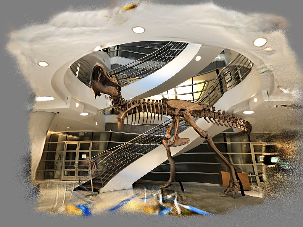
Hash (I)

PE (II)

Hash (II)

PE (III)

Hash (III)

PE (IV)

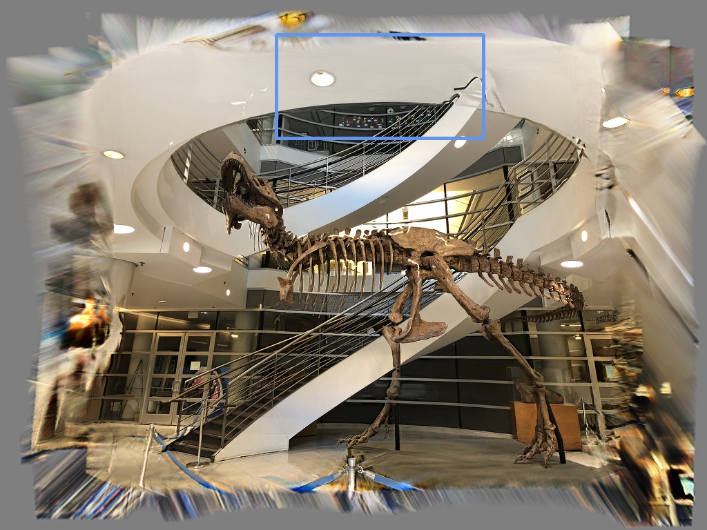
Hash (IV)

PE (V)

Hash (V)

PE (Full)

Hash (Full)

Canonical Image $\phi_{I}$

Canonical View

Canonical Depth

Canonical Image $\phi_{I}$

Canonical View

Canonical Depth

Figure A2: Visualization analysis of the ablation studies for both PE and hash models conducted on the trex scene in the LLFF dataset. Columns A and D are the learned canonical image $\phi_{I}$. Columns B and E are the rendered novel view images at the canonical position (global origin) with the canonical pose (identity rotation). Columns C and F are the corresponding depth maps of the rendered novel views. The zoomed-in patches for subfigure IV-A and Full-A are shown in Fig. A3.

IV: w.o. projection offset $P_{o}$

Full: w. projection offset $P_{o}$

Figure A3: Zoomed-in patches of the canonical images $\phi_{I}$ of the PE model with setting IV (subfigure IV-A) and our full PE model (subfigure Full-A). Without the projection offset, the canonical image fails to include the occluded background ceiling information. Our full model can handle occlusion and naturally aggregate the background ceiling inside the canonical image.

Appendix A Ablation Analysis

The ablation studies (settings I to V) presented in the main paper are conducted for both PE and hash models on the trex scene in the LLFF dataset. In this section, we supply the ablation studies with more corresponding visual analysis, offering more detailed insights. Specifically, we present the reconstruction PSNR statistics in Tab. A1, which match those reported in the main paper. For visual results, Fig. A2 shows the learned canonical image $\phi_{I}$ and the novel viewpoint image with the pseudo canonical camera pose plus its corresponding depth map for each ablation setting. The last row results in Tabs. A1 and A2 indicate that the PE model achieves a satisfactory reconstruction and a superior canonical image $\phi_{I}$ for explicit editing, whereas the hash model excels in terms of reconstruction quality.

Setting I: Replace the explicit density grid $\phi_{G}$ with an implicit one modeled by MLP networks. The learning rate for the replaced implicit density field is set to $10^{-3}$. We can see from Tab. A1 that the reconstruction qualities drop significantly as they fail to learn correct depths as shown by subfigure I-C and I-F in Fig. A2.

Setting II: Replace the explicit canonical image $\phi_{I}$ with an implicit one modeled by MLP networks. The learning rate for the replaced implicit canonical field is also configured to be $10^{-3}$. Based on the findings in Tab. A1, the reconstruction performance of both the PE and hash models experiences degradation of more than $3$ dB and $5$ dB, respectively. Further examination of row II in Fig. A2 reveals that while both models demonstrate satisfactory depth map learning capabilities, they exhibit limited capacities to generate high-quality canonical images for editing purposes.

Table A1: Ablation studies of model components on trex scene. Same as in the main paper.

rowsep=1.2pt colsep=10pt Settings PE Hash I. Implicit density grid $\phi_{G}$ 19.29 18.22 II. Implicit canonical image $\phi_{I}$ 22.53 22.17 III. No initialization $P_{c}$ 23.18 27.56 IV. No offset $P_{o}$ 23.81 23.88 V. No viewdir in offset $P_{o}$ 25.50 26.76 Full model 25.85 27.24

Setting III: Remove the canonical project initialization $P_{c}$ in the projection field $P$. Although in Tab. A1 for setting III, we find that the PE model achieves satisfactory performance and the hash model even performs better than our full hash model in terms of PSNR, the learned canonical images (i.e., subfigure III-A and III-D in Fig. A2) are optimized to be latent color representations instead of natural images, resulting in a loss of editability.

Setting IV: Remove the project offset $P_{o}$ in the projection field $P$. Recall that the learned canonical image $\phi_{I}$ is determined by placing a pseudo canonical camera at the global origin. By comparing subfigure IV-A and Full-A of the PE models, we can see that without having the projection offset, the canonical image (subfigure IV-A) cannot “look through” the foreground ceiling, sharing similar behaviors as the canonical view (column B). However, by adding the projection offset, we enable the capacity of our method to handle occlusions. As demonstrated in subfigure Full-A, the final canonical image $\phi_{I}$ generated by our full models learns to naturally aggregate the occluded background ceiling within the image by leveraging the projection offsets from 3D points to 2D pixels. Please also refer to the corresponding zoomed-in patches in Fig. A3.

Setting V: Remove view dependency in the projection offset $P_{o}$ of the projection field $P$. The omission of viewing directions as the input for projection offset $P_{o}$, as observed from the last two rows in Tabs. A1 and A2, leads to a marginal decrease in reconstruction quality and yields slightly inferior canonical images.

Appendix B Training Details

Our 3D editing pipeline involves a two-step process: (1) we first train a per-scene reconstruction model using the proposed AGAP representation, which includes an explicit density grid $\phi_{G}$, an explicit canonical image $\phi_{I}$, and an associated projection field $\phi_{P}$; (2) we can then perform explicit 2D edits on the canonical image $\phi_{I}$ for 3D scene editing, including scene stylization, content extraction, and texture editing. All experiments, including training on various scenes from different datasets, are conducted and tested on a single RTX A6000 GPU, with specific hyperparameter details outlined in Tab. A2.

Table A2: Hyperparameters for training various scenes in the LLFF [30], Replica [46, 13], and InstructNeRF2NeRF (IN2N) [14] datasets.

rowsep=1.2pt colsep=4.2pt Common PE Models Hash Models Image Size Weight Factor Direction $\mathbf{d}$ Position $\mathbf{p}_{xyz}$ Position $\mathbf{p}_{xyz}$ $\lambda_{uv}$ $\lambda_{tv}$ Type $K$ Anneal Type $K$ Anneal $N_{s}$ $N_{e}$ Type $D$ $K$ Anneal LLFF (768, -) $10^{-5}$ $10^{-5}$ PE 4 ✗ PE 8 ✓ 4000 8000 Hash 2 16 ✗ Replica (768, 1536) $10^{-1}$ $10^{-4}$ PE 4 ✗ PE 8 ✓ 4000 8000 Hash 2 16 ✗ IN2N (768, -) $10^{-5}$ $10^{-5}$ PE 4 ✗ PE 8 ✓ 4000 8000 Hash 2 16 ✗

Optimization. In the first stage, we employ the Adam optimizer [22] to optimize a per-scene model for $60$k steps with an initial learning rate of $0.1$ for both the explicit 3D density grid $\phi_{G}$ and 2D canonical image $\phi_{I}$, and a learning rate of $0.001$ for the implicit projection field $P$ with learnable parameter $\phi_{P}$. The optimization of the entire model involves an objective function comprising three main components: (1) an average $\mathcal{L}_{2}$ photometric loss $\mathcal{L}_{color}$ between the rendered pixel color $\hat{C}(\mathbf{r})$ and the ground-truth color $C(\mathbf{r})$; (2) a projection regularization $\mathcal{L}_{uv}$ aimed at minimizing the projection offset $\Delta\mathbf{p}_{uv}$; and (3) a total variation regularization applied to the density grid $\phi_{G}$.

Weight factor. As stated in the main paper, the final optimization process of our method to model the scene for efficient editing can be formulated as follows:

$$\phi_{G}^{*},\phi_{I}^{*},\phi_{P}^{*}=\operatorname*{arg\,min}_{\phi_{G},\phi_{I},\phi_{P}}{\mathcal{L}_{color}+\mathcal{L}_{uv}+\mathcal{L}_{tv}},$$ (A1)

where the second and the third terms are controlled by their corresponding weight factors $\lambda_{uv}$ and $\lambda_{tv}$, respectively. To be specific, the weight factor $\lambda_{uv}$ is set as $10^{-5}$ for forward-facing scene and $10^{-1}$ for panorama scenes; the weight factor $\lambda_{tv}$ is set as $10^{-5}$ for forward-facing scene and $10^{-4}$ for panorama scenes. Note that for panorama data, we set both the projection and total variation regularization to be relatively large because the depths of indoor scenes in the Replica dataset are sometimes ambiguous due to large walls in the background, where the total variation term is disabled after $20000$ steps to learn depths in details.

Progressive training. Similar to [3, 31, 47], we apply progressive scaling for our voxel grid $\phi_{G}$ and canonical image $\phi_{I}$ for a coarse-to-fine learning process. By gradually refining the resolution of both representations, we enable a more detailed and comprehensive learning process.

At specific scaling-up milestone steps, we increase the $\phi_{G}$ voxel count by a factor of 2 and the $\phi_{I}$ pixel count by a factor of 4. For the forward-facing datasets (i.e., LLFF and InstructNeRF2NeRF), the voxel grid $\phi_{G}$ is scaled up at $\{2000,4000,6000,8000\}$ training steps and the canonical image $\phi_{I}$ is scaled up at $\{8000,16000\}$ training steps. For the panorama Replica dataset, the voxel grid $\phi_{G}$ is scaled up at $\{2000,4000,6000,8000,10000,12000,14000,16000\}$ training steps, and the canonical image $\phi_{I}$ is scaled up at $\{4000,8000,12000,16000\}$ training steps.

Size of voxel grid $\phi_{G}$ and canonical image $\phi_{I}$. After the progressive scaling up, The final resolution of the voxel grid $\phi_{G}$ is set as $384\times 384\times 256$ for forward-facing scenes and $320\times 320\times 320$ for panorama scenes.

In all the experiments, we set the final height $H_{I}$ of the learnable explicit canonical image $\phi_{I}$ as $768$. For panorama data, the canonical image width $W_{I}$ is set to be $1536$ according to the definition of Equirectangular projection. For forward-facing data, the canonical image width $W_{I}$ is adaptively calculated according to the width-height aspect ratio of the training images and the computed bounding box of the scene in NDC space. Denoting the bounding box in NDC space as $(x^{\prime}_{min},x^{\prime}_{max})$ in $x^{\prime}$ dimension, $(y^{\prime}_{min},y^{\prime}_{max})$ in $y^{\prime}$ dimension, and $(z^{\prime}_{min},z^{\prime}_{max})=(-1,1)$ in $z^{\prime}$ dimension and the aspect ratio as $r_{I}$, we can then calculate the canonical image width as:

$$W_{I}=H_{I}\times r_{I}\times\frac{x^{\prime}_{max}-x^{\prime}_{min}}{y^{\prime}_{max}-y^{\prime}_{min}}.$$ (A2)

Annealed positional and hash encoding. The projection offset employs Fourier positional encoding [48] or multi-resolution hash encoding [32] to capture high-frequency information. Given an input vector $\mathbf{x}\in\mathbb{R}^{3}$, the corresponding encoding can be defined as follows:

• The positional encoding is defined as $\gamma_{pe}(\cdot):\mathbb{R}^{3}\to\mathbb{R}^{3\times(1+2K)}$ to encode 3-dimensional vector $\mathbf{x}$ up to $K$ frequencies as $\gamma_{pe}(\mathbf{x})=[\mathbf{x},F_{1}(\mathbf{x}),...,F_{K}(\mathbf{x})]$. For the k-$th$ frequency of positional encoding, we have the encoding function $F_{k}(\mathbf{x})=[\sin(2^{k}\mathbf{x}),\cos(2^{k}\mathbf{x})]\in\mathbb{R}^{2\times 3}$.

• The hash encoding is defined as $\gamma_{h}(\cdot):\mathbb{R}^{3}\to\mathbb{R}^{3+DK}$ to encode the vector $\mathbf{x}$ by a $K$-resolution hash grid with $D$-dimensional feature per layer as $\gamma_{h}(\mathbf{x})=[\mathbf{x},H_{1}(\mathbf{x}),...,H_{K}(\mathbf{x})]$. For the $k$-th resolution hash grid with $D$-dimensional feature at each layer, we have the encoding function $H_{k}(\mathbf{x})\in\mathbb{R}^{D}$.

Motivated by Nerfies [38], the positional or hash encoding can incorporate an optional annealing learning strategy. Specifically, we introduce a weight factor $w^{n}_{k}=\frac{1}{2}(1-\cos(\alpha^{n}_{k}\pi))$ for some encoded frequency $F_{k}^{n}$ or $H_{k}^{n}$ at some training step $n$, such that we have $F_{k}^{n}(\cdot)=w^{n}_{k}F_{k}(\cdot)$ or $H_{k}^{n}(\cdot)=w^{n}_{k}H_{k}(\cdot)$ and

$$\alpha^{n}_{k}=\min(\max(\frac{n-N_{s}}{N_{e}-N_{s}}K-k,0.0),1.0),$$ (A3)

where $N_{s}$ and $N_{e}$ denote the start and end steps for anneal encoding, respectively. The strategy aims to facilitate the learning of low-frequency details and gradually incorporate high-frequency bands as the training progresses.

For all the experiments, the encoding $\gamma_{d}$ of direction $\mathbf{d}$ specifically employs positional encoding $\gamma_{pe}$, where we set $K=4$ with the optional annealing learning strategy off. Concerning the encoding $\gamma_{p}$ of position $\mathbf{p}_{xyz}$, we choose to use positional encoding $\gamma_{pe}$ for PE models and hash encoding $\gamma_{h}$ for hash models, where we set $K=8$ with the annealed learning starting at training step $N_{s}=4000$ and ending at $N_{e}=8000$ for PE models, and we set $D=2$ and $K=16$ without the optional annealed learning strategy for hash models.

References

- Achlioptas et al. [2018] Panos Achlioptas, Olga Diamanti, Ioannis Mitliagkas, and Leonidas J. Guibas. Learning representations and generative models for 3d point clouds. In Proceedings of ICML, 2018.
- Barron et al. [2021] Jonathan T. Barron, Ben Mildenhall, Matthew Tancik, Peter Hedman, Ricardo Martin-Brualla, and Pratul P. Srinivasan. Mip-nerf: A multiscale representation for anti-aliasing neural radiance fields. In Proceedings of ICCV, 2021.
- Barron et al. [2022] Jonathan T. Barron, Ben Mildenhall, Dor Verbin, Pratul P. Srinivasan, and Peter Hedman. Mip-nerf 360: Unbounded anti-aliased neural radiance fields. In Proceedings of CVPR, 2022.
- Brooks et al. [2023] Tim Brooks, Aleksander Holynski, and Alexei A. Efros. Instructpix2pix: Learning to follow image editing instructions. In Proceedings of CVPR, 2023.
- Caron et al. [2021] Mathilde Caron, Hugo Touvron, Ishan Misra, Hervé Jégou, Julien Mairal, Piotr Bojanowski, and Armand Joulin. Emerging properties in self-supervised vision transformers. In Proceedings of ICCV, 2021.
- Chan et al. [2022] Eric R. Chan, Connor Z. Lin, Matthew A. Chan, Koki Nagano, Boxiao Pan, Shalini De Mello, Orazio Gallo, Leonidas J. Guibas, Jonathan Tremblay, Sameh Khamis, Tero Karras, and Gordon Wetzstein. Efficient geometry-aware 3d generative adversarial networks. In Proceedings of CVPR, 2022.
- Chen et al. [2022] Anpei Chen, Zexiang Xu, Andreas Geiger, Jingyi Yu, and Hao Su. Tensorf: Tensorial radiance fields. In Proceedings of ECCV, 2022.
- Chen et al. [2023] Jun-Kun Chen, Jipeng Lyu, and Yu-Xiong Wang. NeuralEditor: Editing neural radiance fields via manipulating point clouds. In Proceedings of CVPR, 2023.
- Deng et al. [2021] Yu Deng, Jiaolong Yang, and Xin Tong. Deformed implicit field: Modeling 3d shapes with learned dense correspondence. In Proceedings of CVPR, 2021.
- Desbrun et al. [2002] Mathieu Desbrun, Mark Meyer, and Pierre Alliez. Intrinsic Parameterizations of Surface Meshes. Computer Graphics Forum, 2002.
- Fridovich-Keil et al. [2022] Sara Fridovich-Keil, Alex Yu, Matthew Tancik, Qinhong Chen, Benjamin Recht, and Angjoo Kanazawa. Plenoxels: Radiance fields without neural networks. In Proceedings of CVPR, 2022.
- Gu et al. [2022] Jiatao Gu, Lingjie Liu, Peng Wang, and Christian Theobalt. Stylenerf: A style-based 3d aware generator for high-resolution image synthesis. In Proceedings of ICLR, 2022.
- Habtegebrial et al. [2022] Tewodros Habtegebrial, Christiano Couto Gava, Marcel Rogge, Didier Stricker, and Varun Jampani. SOMSI: spherical novel view synthesis with soft occlusion multi-sphere images. In Proceedings of CVPR, 2022.
- Haque et al. [2023] Ayaan Haque, Matthew Tancik, Alexei A. Efros, Aleksander Holynski, and Angjoo Kanazawa. Instruct-nerf2nerf: Editing 3d scenes with instructions. In Proceedings of ICCV, 2023.
- Huang et al. [2018] Po-Han Huang, Kevin Matzen, Johannes Kopf, Narendra Ahuja, and Jia-Bin Huang. Deepmvs: Learning multi-view stereopsis. In Proceedings of CVPR, pages 2821–2830, 2018.
- Huang et al. [2022] Yihua Huang, Yue He, Yu-Jie Yuan, Yu-Kun Lai, and Lin Gao. Stylizednerf: Consistent 3d scene stylization as stylized nerf via 2d-3d mutual learning. In Proceedings of CVPR, 2022.
- Ji et al. [2017] Mengqi Ji, Juergen Gall, Haitian Zheng, Yebin Liu, and Lu Fang. Surfacenet: An end-to-end 3d neural network for multiview stereopsis. In Proceedings of ICCV, 2017.
- Kajiya and Herzen [1984] James T. Kajiya and Brian Von Herzen. Ray tracing volume densities. In Proceedings of SIGGRAPH, pages 165–174, 1984.
- Kanazawa et al. [2018] Angjoo Kanazawa, Shubham Tulsiani, Alexei A. Efros, and Jitendra Malik. Learning category-specific mesh reconstruction from image collections. In Proceedings of ECCV, 2018.
- Kasten et al. [2021] Yoni Kasten, Dolev Ofri, Oliver Wang, and Tali Dekel. Layered neural atlases for consistent video editing. TOG, 40(6):210:1–210:12, 2021.
- Kazhdan et al. [2006] Michael M. Kazhdan, Matthew Bolitho, and Hugues Hoppe. Poisson surface reconstruction. In Proceedings of SGP, 2006.
- Kingma and Ba [2015] Diederik P. Kingma and Jimmy Ba. Adam: A method for stochastic optimization. In Proceedings of ICLR, 2015.
- Kirillov et al. [2023] Alexander Kirillov, Eric Mintun, Nikhila Ravi, Hanzi Mao, Chloé Rolland, Laura Gustafson, Tete Xiao, Spencer Whitehead, Alexander C. Berg, Wan-Yen Lo, Piotr Dollár, and Ross B. Girshick. Segment anything. CoRR, abs/2304.02643, 2023.
- Kobayashi et al. [2022] Sosuke Kobayashi, Eiichi Matsumoto, and Vincent Sitzmann. Decomposing nerf for editing via feature field distillation. In Advances in NeurIPS, 2022.
- Lin et al. [2021a] Chen-Hsuan Lin, Wei-Chiu Ma, Antonio Torralba, and Simon Lucey. BARF: bundle-adjusting neural radiance fields. In Proceedings of ICCV, 2021a.
- Lin et al. [2021b] Yen-Chen Lin, Pete Florence, Jonathan T. Barron, Alberto Rodriguez, Phillip Isola, and Tsung-Yi Lin. inerf: Inverting neural radiance fields for pose estimation. In Proceedings of IROS, 2021b.
- Liu et al. [2016] Fayao Liu, Chunhua Shen, Guosheng Lin, and Ian Reid. Learning depth from single monocular images using deep convolutional neural fields. TPAMI, 38(10):2024–2039, 2016.
- Max [1995] Nelson L. Max. Optical models for direct volume rendering. TVCG, 1(2):99–108, 1995.
- Mescheder et al. [2019] Lars M. Mescheder, Michael Oechsle, Michael Niemeyer, Sebastian Nowozin, and Andreas Geiger. Occupancy networks: Learning 3d reconstruction in function space. In Proceedings of CVPR, 2019.
- Mildenhall et al. [2019] Ben Mildenhall, Pratul P. Srinivasan, Rodrigo Ortiz Cayon, Nima Khademi Kalantari, Ravi Ramamoorthi, Ren Ng, and Abhishek Kar. Local light field fusion: practical view synthesis with prescriptive sampling guidelines. TOG, 38(4):29:1–29:14, 2019.
- Mildenhall et al. [2020] Ben Mildenhall, Pratul P. Srinivasan, Matthew Tancik, Jonathan T. Barron, Ravi Ramamoorthi, and Ren Ng. Nerf: Representing scenes as neural radiance fields for view synthesis. In Proceedings of ECCV, pages 405–421, 2020.
- Müller et al. [2022] Thomas Müller, Alex Evans, Christoph Schied, and Alexander Keller. Instant neural graphics primitives with a multiresolution hash encoding. TOG, 41(4):102:1–102:15, 2022.
- Nguyen-Phuoc et al. [2022] Thu Nguyen-Phuoc, Feng Liu, and Lei Xiao. Snerf: stylized neural implicit representations for 3d scenes. TOG, 41(4):142:1–142:11, 2022.
- Oquab et al. [2023] Maxime Oquab, Timothée Darcet, Theo Moutakanni, Huy V. Vo, Marc Szafraniec, Vasil Khalidov, Pierre Fernandez, Daniel Haziza, Francisco Massa, Alaaeldin El-Nouby, Russell Howes, Po-Yao Huang, Hu Xu, Vasu Sharma, Shang-Wen Li, Wojciech Galuba, Mike Rabbat, Mido Assran, Nicolas Ballas, Gabriel Synnaeve, Ishan Misra, Herve Jegou, Julien Mairal, Patrick Labatut, Armand Joulin, and Piotr Bojanowski. Dinov2: Learning robust visual features without supervision. CoRR, arXiv/2304.07193, 2023.
- Ouyang et al. [2023] Hao Ouyang, Qiuyu Wang, Yuxi Xiao, Qingyan Bai, Juntao Zhang, Kecheng Zheng, Xiaowei Zhou, Qifeng Chen, and Yujun Shen. Codef: Content deformation fields for temporally consistent video processing. CoRR, abs/2308.07926, 2023.
- Pang et al. [2023] Hong-Wing Pang, Binh-Son Hua, and Sai-Kit Yeung. Locally stylized neural radiance fields. CoRR, abs/2309.10684, 2023.
- Park et al. [2019] Jeong Joon Park, Peter R. Florence, Julian Straub, Richard A. Newcombe, and Steven Lovegrove. Deepsdf: Learning continuous signed distance functions for shape representation. In Proceedings of CVPR, pages 165–174, 2019.
- Park et al. [2021a] Keunhong Park, Utkarsh Sinha, Jonathan T. Barron, Sofien Bouaziz, Dan B. Goldman, Steven M. Seitz, and Ricardo Martin-Brualla. Nerfies: Deformable neural radiance fields. In Proceedings of ICCV, pages 5845–5854, 2021a.
- Park et al. [2021b] Keunhong Park, Utkarsh Sinha, Peter Hedman, Jonathan T. Barron, Sofien Bouaziz, Dan B. Goldman, Ricardo Martin-Brualla, and Steven M. Seitz. Hypernerf: a higher-dimensional representation for topologically varying neural radiance fields. TOG, 40(6):238:1–238:12, 2021b.
- Reiser et al. [2023] Christian Reiser, Richard Szeliski, Dor Verbin, Pratul P. Srinivasan, Ben Mildenhall, Andreas Geiger, Jonathan T. Barron, and Peter Hedman. MERF: memory-efficient radiance fields for real-time view synthesis in unbounded scenes. TOG, 42(4):89:1–89:12, 2023.
- Rudin et al. [1992] Leonid Rudin, Stanley Osher, and Emad Fatemi. Nonlinear total variation based noise removal algorithms. Physica D: Nonlinear Phenomena, 60(1):259–268, 1992.
- Schönberger and Frahm [2016] Johannes L. Schönberger and Jan-Michael Frahm. Structure-from-motion revisited. In Proceedings of CVPR, 2016.
- Schönberger et al. [2016] Johannes L. Schönberger, Enliang Zheng, Jan-Michael Frahm, and Marc Pollefeys. Pixelwise view selection for unstructured multi-view stereo. In Proceedings of ECCV, 2016.
- Schwarz et al. [2020] Katja Schwarz, Yiyi Liao, Michael Niemeyer, and Andreas Geiger. GRAF: generative radiance fields for 3d-aware image synthesis. In Advances in NeurIPS, 2020.
- Sitzmann et al. [2019] Vincent Sitzmann, Justus Thies, Felix Heide, Matthias Nießner, Gordon Wetzstein, and Michael Zollhöfer. Deepvoxels: Learning persistent 3d feature embeddings. In Proceedings of CVPR, 2019.
- Straub et al. [2019] Julian Straub, Thomas Whelan, Lingni Ma, Yufan Chen, Erik Wijmans, Simon Green, Jakob J. Engel, Raul Mur-Artal, Carl Yuheng Ren, Shobhit Verma, Anton Clarkson, Mingfei Yan, Brian Budge, Yajie Yan, Xiaqing Pan, June Yon, Yuyang Zou, Kimberly Leon, Nigel Carter, Jesus Briales, Tyler Gillingham, Elias Mueggler, Luis Pesqueira, Manolis Savva, Dhruv Batra, Hauke M. Strasdat, Renzo De Nardi, Michael Goesele, Steven Lovegrove, and Richard A. Newcombe. The replica dataset: A digital replica of indoor spaces. CoRR, abs/1906.05797, 2019.
- Sun et al. [2022] Cheng Sun, Min Sun, and Hwann-Tzong Chen. Direct voxel grid optimization: Super-fast convergence for radiance fields reconstruction. In Proceedings of CVPR, pages 5449–5459, 2022.
- Vaswani et al. [2017] Ashish Vaswani, Noam Shazeer, Niki Parmar, Jakob Uszkoreit, Llion Jones, Aidan N. Gomez, Lukasz Kaiser, and Illia Polosukhin. Attention is all you need. In Advances in NeurIPS, pages 5998–6008, 2017.
- Wang et al. [2022] Can Wang, Menglei Chai, Mingming He, Dongdong Chen, and Jing Liao. Clip-nerf: Text-and-image driven manipulation of neural radiance fields. In Proceedings of CVPR, 2022.
- Wang et al. [2019] Jinglu Wang, Bo Sun, and Yan Lu. Mvpnet: Multi-view point regression networks for 3d object reconstruction from A single image. In Proceedings of AAAI, 2019.
- Wang et al. [2018] Nanyang Wang, Yinda Zhang, Zhuwen Li, Yanwei Fu, Wei Liu, and Yu-Gang Jiang. Pixel2mesh: Generating 3d mesh models from single RGB images. In Proceedings of ECCV, 2018.
- Wang et al. [2021a] Peng Wang, Lingjie Liu, Yuan Liu, Christian Theobalt, Taku Komura, and Wenping Wang. Neus: Learning neural implicit surfaces by volume rendering for multi-view reconstruction. In Advances in NeurIPS, 2021a.
- Wang et al. [2023] Qiuyu Wang, Zifan Shi, Kecheng Zheng, Yinghao Xu, Sida Peng, and Yujun Shen. Benchmarking and analyzing 3d-aware image synthesis with a modularized codebase. In Advances in NeurIPS, 2023.
- Wang et al. [2021b] Zirui Wang, Shangzhe Wu, Weidi Xie, Min Chen, and Victor Adrian Prisacariu. Nerf-: Neural radiance fields without known camera parameters. CoRR, abs/2102.07064, 2021b.
- Xiang et al. [2021] Fanbo Xiang, Zexiang Xu, Milos Hasan, Yannick Hold-Geoffroy, Kalyan Sunkavalli, and Hao Su. Neutex: Neural texture mapping for volumetric neural rendering. In Proceedings of CVPR, 2021.
- Yang et al. [2022] Bangbang Yang, Chong Bao, Junyi Zeng, Hujun Bao, Yinda Zhang, Zhaopeng Cui, and Guofeng Zhang. Neumesh: Learning disentangled neural mesh-based implicit field for geometry and texture editing. In Proceedings of ECCV, 2022.
- Yariv et al. [2021] Lior Yariv, Jiatao Gu, Yoni Kasten, and Yaron Lipman. Volume rendering of neural implicit surfaces. In Advances in NeurIPS, 2021.
- Ye et al. [2022] Vickie Ye, Zhengqi Li, Richard Tucker, Angjoo Kanazawa, and Noah Snavely. Deformable sprites for unsupervised video decomposition. In Proceedings of CVPR. IEEE, 2022.
- Yuan et al. [2022] Yu-Jie Yuan, Yang-Tian Sun, Yu-Kun Lai, Yuewen Ma, Rongfei Jia, and Lin Gao. Nerf-editing: Geometry editing of neural radiance fields. In Proceedings of CVPR, 2022.
- Zhang et al. [2022] Kai Zhang, Nicholas I. Kolkin, Sai Bi, Fujun Luan, Zexiang Xu, Eli Shechtman, and Noah Snavely. ARF: artistic radiance fields. In Proceedings of ECCV, 2022.
- Zhang and Agrawala [2023] Lvmin Zhang and Maneesh Agrawala. Adding conditional control to text-to-image diffusion models. In Proceedings of ICCV, 2023.
- Zhang et al. [2023a] Yuechen Zhang, Zexin He, Jinbo Xing, Xufeng Yao, and Jiaya Jia. Ref-npr: Reference-based non-photorealistic radiance fields for controllable scene stylization. In Proceedings of CVPR, 2023a.
- Zhang et al. [2023b] Yanshu Zhang, Shichong Peng, Alireza Moazeni, and Ke Li. PAPR: proximity attention point rendering. In Advances in NeurIPS, 2023b.