Convergence of Multi-Scale Reinforcement Q-Learning Algorithms for Mean Field Game and Control Problems

Abstract

We establish the convergence of the unified two-timescale Reinforcement Learning (RL) algorithm presented in [Angiuli et al., 2022b]. This algorithm provides solutions to Mean Field Game (MFG) or Mean Field Control (MFC) problems depending on the ratio of two learning rates, one for the value function and the other for the mean field term. We focus a setting with finite state and action spaces, discrete time and infinite horizon. The proof of convergence relies on a generalization of the two-timescale approach of [Borkar, 1997]. The accuracy of approximation to the true solutions depends on the smoothing of the policies. We then provide an numerical example illustrating the convergence. Last, we generalize our convergence result to a three-timescale RL algorithm introduced in [Angiuli et al., 2022a] to solve mixed Mean Field Control Games (MFCGs).

1 Introduction

Reinforcement learning (RL) is a type of machine learning technique that enables an agent to learn in an interactive environment by trial and error using feedback from its own actions and experiences, which is formalized through the concept of Markov Decision Process (MDP). For a general introduction, we refer to [Sutton and Barto, 2018]. In the past decade, reinforcement learning has attracted a growing interest and led to several breakthroughs in various fields from classical games, such as Atari [Mnih et al., 2015] or Go [Silver et al., 2016], to robotics (see e.g. [Gu et al., 2017, Vecerik et al., 2017]), and more recently to applications in training models to follow human feedback (see e.g. [Ouyang et al., 2022]). While classical RL focuses on a single agent, multi-agent RL (MARL) aims at extending the paradigm to situations in which multiple agents learn while interacting. We refer to e.g. [Busoniu et al., 2008, Zhang et al., 2021] for more background, and to [Lanctot et al., 2017, Yang and Wang, 2020] for game-theoretic perspectives. Although great successes have been achieved, in particular in classical games, they remain mostly limited to situations with a small number of players. The scalability of model-free MARL methods in terms of the number of agents is a key challenge.

Concurrently, the past decade has witnessed the development of the theory of mean field games (MFGs), introduced by Lasry and Lions [Lasry and Lions, 2007], and Caines, Huang and Malhame [Huang et al., 2006]. MFGs provide a framework to study games with a very large number of anonymous players interacting in a symmetric manner. The theory has been extensively investigated. While the classical concept of MFG focuses on the notion of Nash equilibrium, it can also be relevant to consider the notions of social optimum, which gives rise to so-called mean field control (MFC) problems. We refer to [Bensoussan et al., 2013, Carmona and Delarue, 2018] for more background on this topic.

In the past few years, the question of learning solutions to MFGs and MFC problems using model-free RL methods has gained momentum. Various methods in different settings have been proposed in the literature; see [Laurière et al., 2022] for a survey. With the exception of [Angiuli et al., 2022b], which is the basis of the present paper, these methods focus on solving one of the two types of problems, MFG or MFC. On the one hand, to learn MFGs solutions, two classical families of methods are those relying on strict contraction and fixed point iterations (e.g., [Guo et al., 2019, Cui and Koeppl, 2021, Anahtarci et al., 2023] with tabular Q-learning or deep RL), and those relying on monotonicity and the structure of the game (e.g., [Elie et al., 2020, Perrin et al., 2020, Laurière et al., 2022] using fictitious play and tabular or deep RL). Two-timescale analysis to learn MFG solutions has been used in [Mguni et al., 2018, Subramanian and Mahajan, 2019]. On the other hand, learning solutions to MFC can be amounts to solving an MDP in which the state is the mean field. This leads to value-based RL methods such as Q-learning [Carmona et al., 2019b, Gu et al., 2020]. Other methods include policy gradient [Carmona et al., 2019a] or model-based RL methods [Pasztor et al., 2021].

Recently, [Angiuli et al., 2022b] proposed a common RL algorithm to solve MFGs and MFCs using a single algorithm by adjusting the learning rates. The algorithm iteratively updates an estimation of the population distribution and an estimation of the representative player’s value function. Depending on the rates at which these updates are done, the same algorithm can converge to the MFG solution or the MFC solution. At a high level, the method combines the classical Q-learning updates [Watkins, 1989] with updates of the mean field using a two-timescale scheme. A three-timescale extension has been proposed in [Angiuli et al., 2022a] to learn the solutions of mean field control games (MFCG), which can be interpreted as competitive games between large collaborating groups and the solution as a Nash equilibrium between a large number of such groups.

In this paper, we analyze multi-timescales algorithms that have been introduced and studied numerically in [Angiuli et al., 2022b, Angiuli et al., 2022a] for mean field games, mean field control problems and mixed mean field control games. As in these references, the problems are studied in the context of finite state and action spaces, and in infinite time horizon. The key technical ingredient is the theory of stochastic approximation, see [Borkar, 1997], and in particular results pertaining to multiple timescales. Algorithms used in model-free RL are typically asynchronous and based on samples. To simplify the presentation, we start by analyzing the convergence of an idealized algorithm which uses synchronous and expectation-based updates. We then consider a version where the expected-based updates are replaced by sample-based updates. Last, we study a realistic algorithm, with asynchronous, sample-based updates. Intuitively, each of these two steps corresponds to incorporating one approximation: when the number of samples is large enough, sample-based updates mimic expectation-based updates, and when every state-action pair is visited frequently enough in an asynchronous method, the algorithm’s behavior is close to its synchronous counterparts.

Related works.

As mentioned above, this paper proves the convergence of the algorithms proposed in [Angiuli et al., 2022b, Angiuli et al., 2022a]. The algorithms have been extended to the finite time horizon setting in [Angiuli et al., 2023b] and to deep actor-critic methods in [Angiuli et al., 2023a]. Closely related to this family of methods, learning MFG solutions using RL and multiple timescales has been studied in [Mguni et al., 2018, Subramanian and Mahajan, 2019]. These methods focus purely on he MFG setting, while our method presents a unified algorithm for both MFG and MFC. Besides the multi-timescale aspect, another feature of our work is the fact that the algorithms use the trajectory of a single representative player to learn the asymptotic mean field distribution. Along a similar direction, [Zaman et al., 2023] proposed and analyzed an RL algorithm for MFGs in a setting where the representative agent does not have access to an oracle that can provide the mean field information. Last, the question of approximating the solution to mean field dynamics using the trajectory of a single particle has been studied in [Du et al., 2023b, Du et al., 2023a, Du et al., 2023c], in the continuous space setting.

Structure of the paper.

In Section 2 we introduce notations that will be used throughout the paper. In Sections 3 and 4 respectively, we present the main convergence results for mean field game and mean field control using the idealized algorithm (synchronous updates with expectations). In particular, Theorem 3.11 (resp. Theorem 4.10) proves the convergence and while Theorem 3.13 (resp. Theorem 4.13) analyzes the accuracy in the mean field game setting (resp. mean field control setting). In Section 5, we present an example for which the assumptions are satisfied and we provide a numerical illustration of the unified time-scale algorithm. In Section 6, we extend the convergence analysis to the algorithm with sample-based updates, but still synchronous. Section 7 further extends the analysis to the case of sample-based asynchronous updates. Convergence to mean field control games is presented in Section 8 for a three-timescale extension of the algorithm: Theorems 8.11 and 8.14 analyze respectively the convergence and the accuracy. We conclude the paper in Section 9.

2 Presentation of the model and the algorithm

Notations.

The following notations will be used for both mean field games and mean field control problems. Specific notations will be introduced for mixed mean field control games in Section 8.

Let $\mathcal{{X}}=\{x_{0},\dots,x_{|\mathcal{{X}}|-1}\}$ be a finite state space and $\mathcal{{A}}=\{a_{0},\dots,a_{|\mathcal{{A}}|-1}\}$ be a finite action space. We denote by $\Delta^{|\mathcal{X}|}$ the simplex of probability measures on $\mathcal{X}$. We denote by $\boldsymbol{\delta}$ the indicator function, i.e., for any $x\in\mathcal{X}$, $\boldsymbol{\delta}(x)=[\mathbbm{1}_{x_{0}}(x),...,\mathbbm{1}_{x_{|\mathcal{{X}}|-1}}(x)]$, which is a vector full of $0$ except at the coordinate corresponding to $x$. Let $p$ : $\mathcal{X}\times\mathcal{X}\times\mathcal{A}\times\Delta^{|\mathcal{X}|}\to\Delta^{|\mathcal{X}|}$ be a transition kernel. We will sometimes view it as a function:

$$p:\mathcal{X}\times\mathcal{X}\times\mathcal{A}\times\Delta^{|\mathcal{X}|}\to[0,1],\hskip 20.0pt(x,x^{\prime},a,\mu)\mapsto p(x^{\prime}|x,a,\mu)$$

which will be interpreted as the probability at any given time step to jump to state $x^{\prime}$ starting from state $x$ and using action $a$, when the population distribution is $\mu$.

We will denote by $\mathrm{P}^{\hat{\pi},\hat{\mu}}$ the transition kernel according to the $\hat{\mu}$ and policy ${\hat{\pi}}$, which is defined for any policy $\pi\in\Pi$ and any distributions $\mu,\tilde{\mu}\in\Delta^{|\mathcal{X}|}$ as:

$$(\mathrm{P}^{\pi,\mu}\tilde{\mu})(x)=\sum_{x^{\prime}}\tilde{\mu}(x^{\prime})\sum_{a}\pi(a|x^{\prime})p(x|x^{\prime},a,\mu),\qquad x\in\mathcal{X}.$$ (1)

Let $f$: $\mathcal{X}\times\mathcal{A}\times\Delta^{|\mathcal{X}|}\to\mathbbm{R}$ be a running cost function. We interpret $f(x,a,\mu)$ as the one-step cost, at any given time step, incurred to a representative agent who is at state $x$ and uses action $a$ while the population distribution is $\mu$.

Based on these notations, the notions of mean field game equilibrium and mean field control optimum will be presented in the following sections. For now, let us present the algorithm introduced in [Angiuli et al., 2022b].

Algorithm.

We reproduce [Angiuli et al., 2022b, Algorithm 1] in Algorithm 1. In [Angiuli et al., 2022b], the algorithm was presented with several episodes to help the learning process. Here, to simplify the presentation, we use a single episode. At the beginning of the episode, an initial state $X_{0}$ is provided by the environment. The distribution according to which it is sampled does not matter if the total number of time steps $N_{steps}$ is large enough. Instead of a fixed number of steps, one could stop after a certain stopping criterion is achiever. One possibility is to stop when $\lvert|{\mu_{n+1}-\mu_{n}}\rvert|_{1}\leq tol_{\mu}$ and $\|Q_{n+1}-Q_{n}\|_{1,1}<tol_{Q}$, for some predefined tolerances $tol_{\mu}$ and $tol_{Q}$.

The most important parameters of this algorithm are the learning rates. Our analysis will cover a wider range of possible parameters, but let us recall that in [Angiuli et al., 2022b] chose learning rates of the following specific form, inspired by the RL literature:

$$\rho^{Q}_{n,x,a}=\frac{1}{(1+\nu(x,a,n))^{\omega^{Q}}},\hskip 20.0pt\rho^{\mu}_{n}=\frac{1}{(1+(n+1))^{\omega^{\mu}}}$$

where $\omega^{Q}$ and $\omega^{\mu}$ are two positive constants, and $\nu(x,a,n)=\sum_{m=0}^{n}\mathbbm{1}_{\{(X_{m},A_{m})=(x,a)\}}$ is the number of times the process $(X_{n},A_{n})$ visits state $(x,a)$ up to time $n$.

Algorithm 1 Unified Two-timescale Mean Field Q-learning

0:  $N_{steps}$: number of steps; $\phi$: parameter for $\operatorname*{soft-min}$ policy; $(\rho^{Q}_{n,x,a})_{n,x,a}$: learning rates for the value function; $(\rho^{\mu}_{n})_{n}$: learning rates for the mean field

1:  Initialization: $Q_{0}(x,a)=0$ for all $(x,a)\in\mathcal{{X}}\times\mathcal{{A}}$, $\mu_{0}=[\frac{1}{|\mathcal{{X}}|},...,\frac{1}{|\mathcal{{X}}|}]$

2:  Observe $X_{0}$

3:  Update mean field: $\mu_{0}=\boldsymbol{\delta}(X_{0})$

4:  for $n=0,1,2,\dots,N_{steps}-1$ do

5:     Choose action $A_{n}\sim\operatorname*{soft-min}_{\phi}Q_{n}(X_{n},\cdot)$ Observe cost $f_{n+1}=f(X_{n},A_{n},\mu_{n})$ and state $X_{n+1}\sim p(\cdot|X_{n},A_{n},\mu_{n})$ provided by the environment

6:     Update value function: $Q_{n+1}(x,a)=Q_{n}(x,a)$ for all $(x,a)\neq(X_{n},A_{n})$, and

$$Q_{n+1}(X_{n},A_{n})=Q_{n}(X_{n},A_{n})+\rho^{Q}_{n,X_{n},A_{n}}[f_{n+1}+\gamma\min_{a^{\prime}\in\mathcal{A}}Q_{n}(X_{n+1},a^{\prime})-Q_{n}(X_{n},A_{n})]$$

7:     Update mean field: $\mu_{n+1}=\mu_{n}+\rho^{\mu}_{n}(\boldsymbol{\delta}(X_{n+1})-\mu_{n})$

8:  end for

9:  Return $(\mu_{N_{steps}},Q_{N_{steps}})$

Note that the algorithm uses the cost function $f$ and the transition distribution $p$ only through evaluations and samples respectively. In other words, the algorithm is model-free. Since it only uses samples and not expected values, such updates are sometimes referred to as sample-based updates. Furthermore, at step $n$, the value function $Q_{n+1}$ differs from $Q_{n}$ at only one state-action pair, so the algorithm is asynchronous.

For the analysis, we will start with an idealized version of the algorithm. We will start by considering a synchronous algorithm with expected updates in which, at each iteration, every state-action pair is updated using the expectation of the $Q$-learning updates. We will then consider a version with synchronous but sample-based updates. Finally, we will come back to the algorithm described in Algorithm 1.

Classical Q-learning.

We conclude this section with some background on classical reinforcement learning, since these intuitions will be useful to understand our approach. Classical RL aims at solving a Markov Decision Process (MDP) using the following setting. At each discrete time $n$, the agent observes her state $X_{n}$ and chooses an action $A_{n}$ based on it. Then the environment evolves and provides the agent with a new state $X_{n+1}$ and reports a reward $r_{n+1}$. The goal of the agent is to find the optimal policy $\pi$ such that it assigns to each state the optimal probability of actions in order to maximize the expected cumulative reward. The problem can be recast as the problem of learning the optimal state-action value function, also called Q-function: $Q^{\pi}(x,a)$ represents the expected cumulative discount rewards when starting at state $x$, using an action $a$, and then following policy $\pi$. Mathematically,

$$Q^{\pi}(x,a)=\mathbbm{E}\left[\sum_{n=0}^{\infty}\gamma^{n}r_{n+1}|X_{0}=x,A_{0}=a\right],$$

where $r_{n+1}=r(X_{n},A_{n})$ is the instantaneous reward, $\gamma\in(0,1)$ is a discounting factor, $X_{n+1}$ is distributed according to a transition probability which depends on $X_{n}$ and the action drawn from $\pi(X_{n})$. The goal is to compute the optimal Q-function defined as:

$$Q^{*}(x,a)=\max_{\pi}Q^{\pi}(x,a).$$

To this end, the Q-learning method was introduced by [Watkins, 1989]. The basic idea is to iteratively sample an action $A_{n}\sim\pi(X_{n})$ according to a behavior policy $\pi$, observe the induced state $X_{n+1}$ and reward $r_{n+1}$, and then update the Q-table according to the formula:

$$Q(X_{n},A_{n})\leftarrow Q(X_{n},A_{n})+\rho[r_{n+1}+\gamma\min_{a^{\prime}\in\mathcal{A}}Q(X_{n+1},a^{\prime})-Q(X_{n},A_{n})]$$

where $\rho\in[0,1]$ is a learning rate.

Note that in our case, to be consistent with most of the MFG and MFC literature, we will minimize costs instead of maximizing rewards.

Algorithm 1 can be viewed as a combination of classical Q-learning with an estimation of the mean field term.

3 Mean Field Game

3.1 Mean Field Game Formulation

In the context of Asymptotic MFG introduced in [Angiuli et al., 2022b, Section 2.2], we can view the problem faced by an infinitesimal agent among the crowd as an MDP parameterized by the population distribution. Hence, given a population distribution $\mu$, the Q-function for a single agent can be defined as follows:

$$Q^{\pi}_{\mu}(x,a):=f(x,a,\mu)+\mathbbm{E}\left[\sum_{n\geq 1}\gamma^{n}f(X_{n}^{\pi,\mu},A_{n},\mu)\right],$$ (2)

where the expectation is over the randomness of $X^{\pi,\mu}$ and $A$ such that,

$$\begin{cases}X_{0}^{\pi,\mu}=x,A_{0}=a,\\ X_{n+1}^{\pi,\mu}\sim p(\cdot|X_{n}^{\pi,\mu},A_{n},\mu),\qquad n\geq 0\\ A_{n}\sim\pi(\cdot|X_{n}^{\pi,\mu}),\qquad n\geq 0\end{cases}$$

where $\pi:\mathcal{X}\to\Delta^{|\mathcal{A}|}$ is a mixed policy taking the state $x$ as input and outputting a probability distribution over the action set. We denote by $\Pi$ the set of all such mixed policies.

The optimal Q-function is defined as:

$$Q^{*}_{\mu}(x,a):=\inf_{\pi\in\Pi}Q^{\pi}_{\mu}(x,a).$$ (3)

Since $\mu$ is fixed, Equation (3.20) in [Sutton and Barto, 2018] can be applied, so that it satisfies the Bellman equation:

$$Q^{*}_{\mu}(x,a)=f(x,a,\mu)+\gamma\sum_{x^{\prime}\in\mathcal{X}}p(x^{\prime}|x,a,\mu)\min_{a^{\prime}}Q^{*}_{\mu}(x^{\prime},a^{\prime}).$$ (4)

In short, we denote this Bellman equation (4) by $Q^{*}_{\mu}=\mathcal{B}_{\mu}Q^{*}_{\mu}$, where for every $\mu$, $\mathcal{B}_{\mu}$ is defined for every $Q:\mathcal{X}\times\mathcal{A}\to\mathbb{R}$ as:

$$\mathcal{B}_{\mu}Q:=f(x,a,\mu)+\gamma\sum_{x^{\prime}\in\mathcal{X}}p(x^{\prime}|x,a,\mu)\min_{a^{\prime}}Q(x^{\prime},a^{\prime}).$$

To be more precise, $Q^{*}_{\mu}$ is the fixed point of the Bellman operator $\mathcal{B}_{\mu}$. The Bellman equation (4) implies that there is at least one optimal policy $\pi^{*}$, i.e., such that:

$$Q^{\pi^{*}}_{\mu}(x,a)=Q^{*}_{\mu}(x,a),\qquad\hbox{ for all $(x,a)$.}$$

Indeed, we can take for $\pi^{*}$ any policy such that the support of $\pi^{*}(\cdot|x)$ is included in the set of actions that minimize $Q^{*}_{\mu}(x,\cdot)$. However, there could be multiple optimal policies.

Now we introduce the notion of (mean field) Nash equilibrium.

Definition 3.1.

$(\hat{\mu},\hat{\pi})$ forms a Nash equilibrium if the following two statements hold:

1. (best response) $Q^{\hat{\pi}}_{\hat{\mu}}=Q^{*}_{\hat{\mu}}$

2. (consistency) $\hat{\mu}=\lim_{n\to\infty}\mathcal{L}(X_{n}^{\hat{\pi},\hat{\mu}})$.

To be more precise, the first statement means that $\hat{\pi}$ is optimal for a representative infinitesimal player when the population distribution is $\hat{\mu}$, and the second statement means that $\hat{\mu}$ is a fixed point of the function $\hat{\mu}\mapsto\mathrm{P}^{\hat{\pi},\hat{\mu}}\hat{\mu}$ where $\mathrm{P}^{\hat{\pi},\hat{\mu}}$ is the transition kernel according to the $\hat{\mu}$ and policy ${\hat{\pi}}$, see (1).

3.2 Idealized Two-timescale Approach

In order to solve the problem we defined above, let us first introduce an idealized deterministic two-timescale approach. We consider the following iterative procedure, where both variables are updated at each iteration but with different rates, denoted by $\rho^{\mu}_{n}\in\mathbbm{R}_{+}$ and $\rho^{Q}_{n}\in\mathbbm{R}_{+}$. Starting from an initial guess $(Q_{0},\mu_{0})\in\mathbbm{R}^{|\mathcal{X}|\times|\mathcal{A}|}\times\Delta^{|\mathcal{X}|}$, define iteratively for $n=0,1,\dots$:

$$\begin{cases}\mu_{n+1}=\mu_{n}+\rho_{n}^{\mu}\mathcal{P}_{2}(Q_{n},\mu_{n}),\\ Q_{n+1}=Q_{n}+\rho^{Q}_{n}\mathcal{T}_{2}(Q_{n},\mu_{n}),\end{cases}$$ (5)

where the functions $\mathcal{P}_{2}:\mathbb{R}^{|\mathcal{X}|\times|\mathcal{A}|}\to\Delta^{|\mathcal{X}|}$ and $\mathcal{P}_{2}:\mathbb{R}^{|\mathcal{X}|\times|\mathcal{A}|}\to\mathbb{R}^{|\mathcal{X}|\times|\mathcal{A}|}$ are defined by:

$$\begin{cases}\mathcal{P}_{2}(Q,\mu)(x)=\sum_{x^{\prime}}\mu(x^{\prime})p(x|x^{\prime},\operatorname*{soft-min}_{\phi}Q(x^{\prime}),\mu)-\mu(x),\\ \mathcal{T}_{2}(Q,\mu)(x,a)=f(x,a,\mu)+\gamma\sum_{x^{\prime}}p(x^{\prime}|x,a,\mu)\min_{a^{\prime}}Q(x^{\prime},a^{\prime})-Q(x,a).\end{cases}$$

These two functions can also be expressed in the following way:

$$\begin{cases}\mathcal{P}_{2}(Q,\mu)=\mathrm{P}^{\operatorname*{soft-min}_{\phi}Q,\mu}\mu-\mu,\\ \mathcal{T}_{2}(Q,\mu)=\mathcal{B}_{\mu}Q-Q.\end{cases}$$

Our proof requires the functions $\mathcal{T}_{2}$ and $\mathcal{P}_{2}$ to be Lipschitz continuous. In order to obtain this property, we use $\operatorname*{soft-min}_{\phi}$ instead of $\arg\min$ under function $\mathcal{P}_{2}$ and we require Lipschitz continuity of $f$. By [Borkar, 1997], we will obtain that, if $\rho^{\mu}_{n}/\rho^{Q}_{n}\to 0$ as $n\to+\infty$, the solution $(\mu_{n},Q_{n})_{n}$ to the above iterations (5) has a behavior that is described (in a sense to be made precise later) by the following system of ODEs, in the regime where $\epsilon$ is small and $t$ goes to infinity:

$$\begin{cases}\dot{\mu}_{t}=\mathcal{P}_{2}(Q_{t},\mu_{t}),\\ \dot{Q}_{t}=\frac{1}{\epsilon}\mathcal{T}_{2}(Q_{t},\mu_{t}),\end{cases}$$ (6)

where $\rho^{\mu}_{n}/\rho^{Q}_{n}$ is thought of being of order $\epsilon<<1$.

3.3 Convergence of Idealized Two-timescale Approach

In this section, we will establish the convergence of the idealized two-timescale approach defined in (5).

We introduce the following assumption.

Assumption 3.2.

The cost function $f$ is bounded and is Lipschitz with respect to $\mu$, with Lipschitz constant denoted by $L_{f}$ when using the $L^{1}$ norm. The transition kernel $p(\cdot|\cdot,\cdot,\mu)$ is also Lipschitz with respect to $\mu$, with Lipschitz constant denoted by $L_{p}$ when using the $L^{1}$ norm. In other words, for every $x,a,\mu,\mu^{\prime}$,

$$|f(x,a,\mu)-f(x,a,\mu^{\prime})| \leq L_{f}\|\mu-\mu^{\prime}\|_{1}=L_{f}\sum_{x}|\mu(x)-\mu^{\prime}(x)|,$$

$$\sum_{x^{\prime}}|p(x^{\prime}|x,a,\mu)-p(x^{\prime}|x,a,\mu^{\prime})|=\|p(\cdot|x,a,\mu)-p(\cdot|x,a,\mu^{\prime})\|_{1} \leq L_{p}\|\mu-\mu^{\prime}\|_{1}=L_{p}\sum_{x}|\mu(x)-\mu^{\prime}(x)|.$$

Under Assumption 3.2, we now show that the functions $\mathcal{P}_{2}$ and $\mathcal{T}_{2}$ are Lipschitz continuous.

Proposition 3.3.

If Assumption 3.2 holds, then the function $(Q,\mu)\mapsto\mathcal{P}_{2}(Q,\mu)$ is Lipschitz with respect to both $Q$ and $\mu$:

$$\|\mathcal{P}_{2}(Q,\mu)-\mathcal{P}_{2}(Q^{\prime},\mu)\|_{\infty}\leq c_{max}\phi|\mathcal{A}|\|Q-Q^{\prime}\|_{\infty},$$ (7)

where $c_{max}:=\max_{x,x^{\prime},a,\mu}p(x|x^{\prime},a,\mu)$ and

$$\|\mathcal{P}_{2}(Q,\mu)-\mathcal{P}_{2}(Q,\mu^{\prime})\|_{\infty}\leq(L_{p}+2-|\mathcal{X}|c_{min}^{\phi})\|\mu-\mu^{\prime}\|_{1}\leq(L_{p}+2-|\mathcal{X}|c_{min})\|\mu-\mu^{\prime}\|_{1},$$ (8)

where

$$c_{min}^{\phi}:= \min_{x,x^{\prime},Q,\mu}\mathrm{P}^{\operatorname*{soft-min}_{\phi}Q,\mu}(x^{\prime},x)=\min_{x,x^{\prime},Q,\mu}\sum_{a}{\operatorname*{soft-min}}_{\phi}Q(x^{\prime},a)p(x|x^{\prime},a,\mu)$$

$$\geq\min_{x,x^{\prime},a,\mu}p(x|x^{\prime},a,\mu)\sum_{a}{\operatorname*{soft-min}}_{\phi}Q(x^{\prime},a)=\min_{x,x^{\prime},a,\mu}p(x|x^{\prime},a,\mu)=:c_{min}$$

Proof.

$$\|\mathcal{P}_{2}(Q,\mu)-\mathcal{P}_{2}(Q^{\prime},\mu)\|_{1} =\|\mathrm{P}^{\operatorname*{soft-min}_{\phi}Q,\mu}\mu-\mathrm{P}^{\operatorname*{soft-min}_{\phi}Q^{\prime},\mu}\mu\|_{\infty}$$

$$\leq\sum_{x}|\sum_{x^{\prime}}\mu(x^{\prime})\sum_{a}(({\operatorname*{soft-min}}_{\phi}Q(x^{\prime}))(a)p(x|x^{\prime},a,\mu)-({\operatorname*{soft-min}}_{\phi}Q^{\prime}(x^{\prime}))(a)p(x|x^{\prime},a,\mu))|$$

$$\leq\sum_{x^{\prime}}\mu(x^{\prime})|\sum_{a}\sum_{x}(({\operatorname*{soft-min}}_{\phi}Q(x^{\prime}))(a)p(x|x^{\prime},a,\mu)-({\operatorname*{soft-min}}_{\phi}Q^{\prime}(x^{\prime}))(a)p(x|x^{\prime},a,\mu))|$$

$$\leq\sum_{x^{\prime}}\mu(x^{\prime})\sqrt{\sum_{a}1^{2}}\|{\operatorname*{soft-min}}_{\phi}Q(x^{\prime})-{\operatorname*{soft-min}}_{\phi}Q^{\prime}(x^{\prime})\|_{2}$$

$$\leq\sum_{x^{\prime}}\mu(x^{\prime})|\mathcal{A}|^{\frac{1}{2}}\phi\|Q(x^{\prime})-Q^{\prime}(x^{\prime})\|_{2}$$

$$\leq|\mathcal{A}|^{\frac{1}{2}}\phi\sum_{x^{\prime}}\mu(x^{\prime})\|Q(x^{\prime})-Q^{\prime}(x^{\prime})\|_{2}$$

$$\leq|\mathcal{A}|\phi\sum_{x^{\prime}}\mu(x^{\prime})\|Q(x^{\prime})-Q^{\prime}(x^{\prime})\|_{\infty}$$

$$\leq\phi|\mathcal{A}|\|Q-Q^{\prime}\|_{\infty},$$

and,

$$\|\mathcal{P}_{2}(Q,\mu)-\mathcal{P}_{2}(Q,\mu^{\prime})\|_{\infty} \leq\|\mathrm{P}^{\operatorname*{soft-min}_{\phi}Q,\mu}\mu-\mathrm{P}^{\operatorname*{soft-min}_{\phi}Q,\mu^{\prime}}\mu^{\prime}\|_{\infty}+\|\mu-\mu^{\prime}\|_{\infty}$$

$$\leq\|\mathrm{P}^{\operatorname*{soft-min}_{\phi}Q,\mu}\mu-\mathrm{P}^{\operatorname*{soft-min}_{\phi}Q,\mu}\mu^{\prime})\|_{1}+\|\mathrm{P}^{\operatorname*{soft-min}_{\phi}Q,\mu}\mu^{\prime}-\mathrm{P}^{\operatorname*{soft-min}_{\phi}Q,\mu^{\prime}}\mu^{\prime}\|_{1}+\|\mu-\mu^{\prime}\|_{1}$$

$$\leq(1-|\mathcal{X}|c_{min}^{\phi})\|\mu-\mu^{\prime}\|_{1}+L_{p}\|\mu-\mu^{\prime}\|_{1}+\|\mu-\mu^{\prime}\|_{1}$$

$$\leq(L_{p}+2-|\mathcal{X}|c_{min}^{\phi})\|\mu-\mu^{\prime}\|_{1}$$

$$\leq(L_{p}+2-|\mathcal{X}|c_{min})\|\mu-\mu^{\prime}\|_{1}.$$

For the first term in the right-hand side after the second inequality, the idea is that we can find $p(i,j)>\epsilon$, so that $1-N\epsilon>0$, then define $q(i,j)=(p(i,j)-\epsilon)/(1-N\epsilon)$. Then $P=(1-N\epsilon)Q+\epsilon J$, where $J$ is $N\times N$ matrix with all entries 1. Finally we use this fact to calculate the total variation. ∎

Proposition 3.4.

If Assumption 3.2 holds, The function $(Q,\mu)\mapsto\mathcal{T}_{2}(Q,\mu)$ is Lipschitz with respect to both $Q$ and $\mu$.

Proof.

$$\|\mathcal{T}_{2}(Q,\mu)-\mathcal{T}_{2}(Q^{\prime},\mu)\|_{\infty} \leq\|\mathcal{B}_{\mu}Q-\mathcal{B}_{\mu}Q^{\prime}\|_{\infty}+\|Q-Q^{\prime}\|_{\infty}$$

$$\leq\gamma\|\sum_{x^{\prime}}p(x^{\prime}|\cdot,\cdot,\mu)(\min_{a^{\prime}}Q(x^{\prime},a^{\prime})-\min_{a^{\prime}}Q^{\prime}(x^{\prime},a^{\prime}))\|_{\infty}+\|Q-Q^{\prime}\|_{\infty}$$

$$\leq\gamma\|Q-Q^{\prime}\|_{\infty}+\|Q-Q^{\prime}\|_{\infty}$$

$$\leq(\gamma+1)\|Q-Q^{\prime}\|_{\infty},$$

where we used the fact that

$$\|\sum_{x^{\prime}}p(x^{\prime}|\cdot,\cdot,\mu)(\min_{a^{\prime}}Q(x^{\prime},a^{\prime})-\min_{a^{\prime}}Q^{\prime}(x^{\prime},a^{\prime}))\|_{\infty}\leq\sup_{x,a}\sum_{x^{\prime}}p(x^{\prime}|x,a,\mu)\|(\min_{a^{\prime}}Q(x^{\prime},a^{\prime})-\min_{a^{\prime}}Q^{\prime}(x^{\prime},a^{\prime}))\|_{\infty},$$

with $p(x^{\prime}|x,a,\mu)\leq 1$ and $\|(\min_{a^{\prime}}Q(x^{\prime},a^{\prime})-\min_{a^{\prime}}Q^{\prime}(x^{\prime},a^{\prime}))\|_{\infty}\leq\|Q-Q^{\prime}\|_{\infty}$.

$$\|\mathcal{T}_{2}(Q,\mu)-\mathcal{T}_{2}(Q,\mu^{\prime})\|_{\infty} \leq\|f(\cdot,\cdot,\mu)-f(\cdot,\cdot,\mu^{\prime})\|_{\infty}+\|\gamma\sum_{x^{\prime}}|p(x^{\prime}|\cdot,\cdot,\mu)-p(x^{\prime}|\cdot,\cdot,\mu^{\prime})||\min_{a^{\prime}}Q(x^{\prime},a^{\prime})|\|_{\infty}$$

$$\leq(L_{f}+\gamma L_{p}\|Q\|_{\infty})\|\mu-\mu^{\prime}\|_{1}$$

$$\leq|\mathcal{X}|(L_{f}+\gamma L_{p}\|Q\|_{\infty})\|\mu-\mu^{\prime}\|_{\infty}.$$

∎

Now that we have these Lipschitz properties, we show that the O.D.E. system (5) has a unique global asymptotically stable equilibrium (GASE).

Proposition 3.5.

If Assumption 3.2 holds, then for any given $\mu$, $\dot{Q}_{t}=\mathcal{T}_{2}(Q_{t},\mu)$ has a unique GASE, that we will denote by $Q^{*}_{\mu}$. Moreover, $Q^{*}_{\mu}:\Delta^{|\mathcal{X}|}\to\mathbbm{R}^{|\mathcal{X}|\times|\mathcal{A}|}$ is Lipchitz.

Proof.

We will use in the proof the fact that, by definition of the $Q$ table, $\|Q^{*}_{\mu}\|_{\infty}\leq\frac{1}{1-\gamma}\|f\|_{\infty}$. By the procedure we used to prove Proposition 3.4, we have $\|\mathcal{B}_{\mu}Q-\mathcal{B}_{\mu}Q^{\prime}\|_{\infty}\leq\gamma\|Q-Q^{\prime}\|_{\infty}$, where $\gamma<1$ implies that $Q\mapsto\mathcal{B}_{\mu}Q$ is a strict contraction. As a result, by contraction mapping theorem [Sell, 1973], a unique GASE exists and furthermore by [Borkar and Soumyanatha, 1997, Theorem 3.1], $Q_{t}$ will converge to it. We denote it by $Q^{*}_{\mu}$. Then,

$$\|Q^{*}_{\mu}-Q^{*}_{\mu^{\prime}}\|_{\infty} =\|\mathcal{B}_{\mu}Q^{*}_{\mu}-\mathcal{B}_{\mu^{\prime}}Q^{*}_{\mu^{\prime}}\|_{\infty}$$

$$\leq\|\mathcal{B}_{\mu}Q^{*}_{\mu}-\mathcal{B}_{\mu^{\prime}}Q^{*}_{\mu}\|_{\infty}+\|\mathcal{B}_{\mu^{\prime}}Q^{*}_{\mu}-\mathcal{B}_{\mu^{\prime}}Q^{*}_{\mu^{\prime}}\|_{\infty}$$

$$\leq\|\mathcal{T}_{2}(Q^{*}_{\mu},\mu)-\mathcal{T}_{2}(Q^{*}_{\mu},\mu^{\prime})\|_{\infty}+\gamma\|Q^{*}_{\mu}-Q^{*}_{\mu^{\prime}}\|_{\infty}$$

$$\leq|\mathcal{X}|(L_{f}+\gamma L_{p}\|Q^{*}_{\mu}\|_{\infty})\|\mu-\mu^{\prime}\|_{\infty}+\gamma\|Q^{*}_{\mu}-Q^{*}_{\mu^{\prime}}\|_{\infty}$$

$$\leq|\mathcal{X}|(L_{f}+\frac{\gamma}{1-\gamma}L_{p}\|f\|_{\infty})\|\mu-\mu^{\prime}\|_{\infty}+\gamma\|Q^{*}_{\mu}-Q^{*}_{\mu^{\prime}}\|_{\infty}$$

As a result, we have $\|Q^{*}_{\mu}-Q^{*}_{\mu^{\prime}}\|_{\infty}\leq\frac{L_{f}|\mathcal{X}|+\frac{\gamma}{1-\gamma}L_{p}\|f\|_{\infty}|\mathcal{X}|}{1-\gamma}\|\mu-\mu^{\prime}\|_{\infty}$, which is uniformly Lipschitz with respect to $\mu$. ∎

To prove that the GASE exists for the first O.D.E. in (6), we need to control $\phi$ properly to have the strict contraction so that we introduce the assumptions below.

Assumption 3.6.

We assume $L_{p}<|\mathcal{X}|c_{min}$.

Assumption 3.7.

We assume $0<\phi<\frac{|\mathcal{X}|c_{min}-L_{p}}{|\mathcal{A}|}\frac{1-\gamma}{L_{f}+\frac{\gamma}{1-\gamma}L_{p}\|f\|_{\infty}}=:\phi_{max}$.

With this assumption, we have $(\phi|\mathcal{A}|\frac{L_{f}+\frac{\gamma}{1-\gamma}L_{p}\|f\|_{\infty}}{1-\gamma}+L_{p}+1-|\mathcal{X}|c_{min})<1$. Also we have $(\phi|\mathcal{A}|\frac{L_{f}+\gamma L_{p}\|Q^{*}_{\mu}\|_{\infty}}{1-\gamma}+L_{p}+1-|\mathcal{X}|c_{min})<1$, which will give the strict contraction property we need in the next proposition.

Proposition 3.8.

Under Assumptions 3.2, 3.6 and 3.7, $\dot{\mu}_{t}=\mathcal{P}_{2}(Q^{*}_{\mu_{t}},\mu_{t})$ has a unique GASE, that we will denote by $\mu^{*\phi}$.

Proof.

We show that $\mu\mapsto\mathrm{P}^{\operatorname*{soft-min}_{\phi}Q^{*}_{\mu},\mu}\mu$ is a strict contraction. First, recall that, from Proposition 3.3, we have

$$\|\mathrm{P}^{\operatorname*{soft-min}_{\phi}Q,\mu}\mu-\mathrm{P}^{\operatorname*{soft-min}_{\phi}Q,\mu^{\prime}}\mu^{\prime}\|_{1} \leq\|\mathrm{P}^{\operatorname*{soft-min}_{\phi}Q,\mu}\mu-\mathrm{P}^{\operatorname*{soft-min}_{\phi}Q,\mu}\mu^{\prime})\|_{1}+\|\mathrm{P}^{\operatorname*{soft-min}_{\phi}Q,\mu}\mu^{\prime}-\mathrm{P}^{\operatorname*{soft-min}_{\phi}Q,\mu^{\prime}}\mu^{\prime}\|_{1}$$

$$\leq(1-|\mathcal{X}|c_{min}^{\phi})\|\mu-\mu^{\prime}\|_{1}+L_{p}\|\mu-\mu^{\prime}\|_{1}$$

$$\leq(1+L_{p}-|\mathcal{X}|c_{min})\|\mu-\mu^{\prime}\|_{1}.$$

We have:

$$\|\mathrm{P}^{\operatorname*{soft-min}_{\phi}Q^{*}_{\mu},\mu}\mu-\mathrm{P}^{\operatorname*{soft-min}_{\phi}Q^{*}_{\mu^{\prime}},\mu^{\prime}}\mu^{\prime}\|_{1}$$

$$\leq\|\mathrm{P}^{\operatorname*{soft-min}_{\phi}Q^{*}_{\mu},\mu}\mu-\mathrm{P}^{\operatorname*{soft-min}_{\phi}Q^{*}_{\mu^{\prime}},\mu}\mu\|_{1}+\|\mathrm{P}^{\operatorname*{soft-min}_{\phi}Q^{*}_{\mu^{\prime}},\mu}\mu-\mathrm{P}^{\operatorname*{soft-min}_{\phi}Q^{*}_{\mu^{\prime}},\mu^{\prime}}\mu^{\prime}\|_{1}$$

$$\leq\|\mathcal{P}_{2}(Q^{*}_{\mu},\mu)-\mathcal{P}_{2}(Q^{*}_{\mu^{\prime}},\mu)\|_{1}+\|\mathrm{P}^{\operatorname*{soft-min}_{\phi}Q^{*}_{\mu^{\prime}},\mu}\mu-\mathrm{P}^{\operatorname*{soft-min}_{\phi}Q^{*}_{\mu^{\prime}},\mu^{\prime}}\mu^{\prime}\|_{1}$$

$$\leq\|\mathcal{P}_{2}(Q^{*}_{\mu},\mu)-\mathcal{P}_{2}(Q^{*}_{\mu^{\prime}},\mu)\|_{1}++(1+L_{p}-|\mathcal{X}|c_{min})\|\mu-\mu^{\prime}\|_{1}$$

$$\leq\phi|\mathcal{A}|\|Q^{*}_{\mu}-Q^{*}_{\mu^{\prime}}\|_{\infty}+(1+L_{p}-|\mathcal{X}|c_{min})\|\mu-\mu^{\prime}\|_{1}$$

$$\leq(\phi|\mathcal{A}|\frac{L_{f}+\gamma L_{p}\|Q^{*}_{\mu}\|_{\infty}}{1-\gamma}+L_{p}+1-|\mathcal{X}|c_{min})\|\mu-\mu^{\prime}\|_{1},$$

which shows the strict contraction property. As a result, by contraction mapping theorem [Sell, 1973], a unique GASE exists and furthermore by [Borkar and Soumyanatha, 1997, Theorem 3.1], $\mu_{t}$ will converge to it. ∎

Remark 3.9.

If instead, we assume (or we can prove) the unique GASE in Proposition 3.8 exists, then Assumptions 3.6 and 3.7 are not needed, which means that we can take any $\phi\geq 0$ without the upper bound restriction. The same remark applies to the following results.

With the above propositions, we can now introduce our first theorem, which guarantees the convergence of the idealized two-timescale approach. It relies on the following assumptions about the update rates:

Assumption 3.10.

The learning rate $\rho^{Q}_{n}$ and $\rho^{\mu}_{n}$ are sequences of positive real numbers satisfying

$$\sum_{n}\rho^{Q}_{n}=\sum_{n}\rho^{\mu}_{n}=\infty,\qquad\sum_{n}|\rho^{Q}_{n}|^{2}+|\rho^{\mu}_{n}|^{2}<\infty,\qquad\rho^{\mu}_{n}/\rho^{Q}_{n}\xrightarrow[n\to+\infty]{}0.$$

Theorem 3.11.

Under Assumptions 3.2, 3.6, 3.7 and 3.10, $(\mu_{n},Q_{n})$ defined in (5) converges to $(\mu^{*\phi},Q^{*}_{\mu^{*\phi}})$ as $n\to\infty$.

Proof.

With Assumptions 3.2, 3.6, 3.7 and 3.10, and the results of Propositions 3.3, 3.4, 3.5 and 3.8, the assumptions of [Borkar, 1997, Theorem 1.1] are satisfied. This result guarantees the convergence in the statement. ∎

Next, we show that the limit point is an approximation of the MFG solution. In order to do it, we need to introduce the assumption below,

Assumption 3.12.

We assume the following system of equations has a unique solution:

$$\begin{cases}\hat{\mu}=\mathrm{P}^{\hat{\pi},\hat{\mu}}\hat{\mu},\\ Q^{*}_{\hat{\mu}}=Q^{\hat{\pi}}_{\hat{\mu}}\\ \hat{\pi}=\operatorname*{argmin-e}_{e}Q^{*}_{\hat{\mu}}.\end{cases}$$ (9)

The interpretation of (9) is the following. The first equation says that $\hat{\mu}$ is the stationary distribution obtained when the whole population is using the policy $\hat{\pi}=\operatorname*{argmin-e}_{e}Q^{*}_{\hat{\mu}}$. The second equation says that $Q^{*}_{\hat{\mu}}$ is the optimal value function of a representative player. Overall, this implies that $(\hat{\mu},\hat{\pi})$ form an MFG equilibrium (see Definition 3.1).

Theorem 3.13.

Suppose Assumptions 3.10, 3.2, 3.6, 3.7 and 3.12. Let $(\hat{\mu},Q^{*}_{\hat{\mu}})$ be the solution of (9). Let $\delta$ be the action gap defined as $\delta=\min_{x\in\mathcal{X}}(\min_{a\notin\arg\min_{a}Q^{*}_{\hat{\mu}}}Q^{*}_{\hat{\mu}}(x,a)-\min_{a}Q^{*}_{\hat{\mu}}(x,a))>0$, and $\delta=\infty$ if $Q^{*}_{\hat{\mu}}(x)$ is constant with respect to $a$ for each $x$. Assume $\phi_{max}-\frac{1}{\delta}>0$. Then:

$$\begin{cases}\|\mu^{*\phi}-\hat{\mu}\|_{1}\leq\frac{2|\mathcal{A}|^{\frac{1}{2}}(1-\gamma)\exp(-\phi\delta)}{(L_{f}+\frac{\gamma}{1-\gamma}L_{p}\|f\|_{\infty})(\phi_{max}-\phi)}\\ \|Q^{*}_{\mu^{*\phi}}-Q^{*}_{\hat{\mu}}\|_{\infty}\leq\frac{2|\mathcal{A}|^{\frac{1}{2}}\exp(-\phi\delta)}{\phi_{max}-\phi}.\end{cases}$$ (10)

Proof.

We consider the errors separately. First,

$$\|\mu^{*\phi}-\hat{\mu}\|_{1} =\|\mathrm{P}^{\operatorname*{soft-min}_{\phi}Q^{*}_{\mu^{*\phi}},\mu^{*\phi}}\mu^{*\phi}-\mathrm{P}^{\operatorname*{argmin-e}_{e}Q^{*}_{\hat{\mu}},\hat{\mu}}\hat{\mu}\|_{1}$$

$$\leq\|\mathrm{P}^{\operatorname*{soft-min}_{\phi}Q^{*}_{\mu^{*\phi}},\mu^{*\phi}}\mu^{*\phi}-\mathrm{P}^{\operatorname*{soft-min}_{\phi}Q^{*}_{\hat{\mu}},\mu^{*\phi}}\mu^{*\phi}\|_{1}$$

$$\hskip 14.22636pt+\|\mathrm{P}^{\operatorname*{soft-min}_{\phi}Q^{*}_{\hat{\mu}},\mu^{*\phi}}\mu^{*\phi}-\mathrm{P}^{\operatorname*{argmin-e}_{e}Q^{*}_{\hat{\mu}},\mu^{*\phi}}\mu^{*\phi}\|_{1}+\|\mathrm{P}^{\operatorname*{argmin-e}_{e}Q^{*}_{\hat{\mu}},\mu^{*\phi}}\mu^{*\phi}-\mathrm{P}^{\operatorname*{argmin-e}_{e}Q^{*}_{\hat{\mu}},\hat{\mu}}\hat{\mu}\|_{1}$$

$$\leq\phi|\mathcal{A}|\|Q^{*}_{\mu^{*\phi}}-Q^{*}_{\hat{\mu}}\|_{\infty}+|\mathcal{A}|^{\frac{1}{2}}\max_{x\in\mathcal{X}}\|{\operatorname*{soft-min}}_{\phi}Q^{*}_{\hat{\mu}}(x)-\operatorname*{argmin-e}_{e}Q^{*}_{\hat{\mu}}(x)\|_{2}$$

$$\hskip 14.22636pt+(L_{p}+1-|\mathcal{X}|c_{min})\|\mu^{*\phi}-\hat{\mu}\|_{1}$$

$$\leq\phi|\mathcal{A}|\|Q^{*}_{\mu^{*\phi}}-Q^{*}_{\hat{\mu}}\|_{\infty}+2|\mathcal{A}|^{\frac{3}{2}}\exp(-\phi\delta)+(L_{p}+1-|\mathcal{X}|c_{min})\|\mu^{*\phi}-\hat{\mu}\|_{1},$$

where the second inequality uses Proposition 3.3, and the last line is by [Guo et al., 2019, Lemma 7] and $\delta=\min_{x\in\mathcal{X}}(\min_{a\notin\arg\min_{a}Q^{*}_{\hat{\mu}}}Q^{*}_{\hat{\mu}}(x,a)-\min_{a}Q^{*}_{\hat{\mu}}(x,a)\color[rgb]{0,0,0})>0$, and $\delta=\infty$ if $Q^{*}_{\hat{\mu}}(x,a)$ is constant with respect to $a$ for each $x$.

This implies that $\|\mu^{*\phi}-\hat{\mu}\|_{1}\leq\frac{\phi|\mathcal{A}|\|Q^{*}_{\mu^{*\phi}}-Q^{*}_{\hat{\mu}}\|_{\infty}+2|\mathcal{A}|^{\frac{3}{2}}\exp(-\phi\delta)}{(|\mathcal{X}|c_{min}-L_{p})}$. Then, by $\|Q^{*}_{\mu^{*\phi}}-Q^{*}_{\hat{\mu}}\|_{\infty}\leq\frac{L_{f}+\frac{\gamma}{1-\gamma}L_{p}\|f\|_{\infty}}{1-\gamma}\|\mu^{*\phi}-\hat{\mu}\|_{1}$, we have

$$((|\mathcal{X}|c_{min}-L_{p})-\frac{\phi|\mathcal{A}|(L_{f}+\frac{\gamma}{1-\gamma}L_{p}\|f\|_{\infty})}{1-\gamma})\|\mu^{*\phi}-\hat{\mu}\|_{1}\leq 2|\mathcal{A}|^{\frac{3}{2}}\exp(-\phi\delta).$$

So that, we have,

$$\begin{cases}\|\mu^{*\phi}-\hat{\mu}\|_{1}\leq\frac{2|\mathcal{A}|^{\frac{3}{2}}\exp(-\phi\delta)}{((|\mathcal{X}|c_{min}-L_{p})-\frac{\phi|\mathcal{A}|(L_{f}+\frac{\gamma}{1-\gamma}L_{p}\|f\|_{\infty})}{1-\gamma})}=\frac{2|\mathcal{A}|^{\frac{1}{2}}(1-\gamma)\exp(-\phi\delta)}{(L_{f}+\frac{\gamma}{1-\gamma}L_{p}\|f\|_{\infty})(\phi_{max}-\phi)}\\ \|Q^{*}_{\mu^{*\phi}}-Q^{*}_{\hat{\mu}}\|_{\infty}\leq\frac{2|\mathcal{A}|^{\frac{3}{2}}(L_{f}+\frac{\gamma}{1-\gamma}L_{p}\|f\|_{\infty})\exp(-\phi\delta)}{((1-\gamma)(|\mathcal{X}|c_{min}-L_{p})-\phi|\mathcal{A}|(L_{f}+\frac{\gamma}{1-\gamma}L_{p}\|f\|_{\infty})}=\frac{2|\mathcal{A}|^{\frac{1}{2}}\exp(-\phi\delta)}{\phi_{max}-\phi}.\end{cases}$$ (11)

Recall by Assumptions 3.6 and 3.7, we have $((|\mathcal{X}|c_{min}-L_{p})-\frac{\phi|\mathcal{A}|(L_{f}+\frac{\gamma}{1-\gamma}L_{p}\|f\|_{\infty})}{1-\gamma})>0$, then we will have by taking $\phi=\frac{|\mathcal{X}|c_{min}-L_{p}}{|\mathcal{A}|}\frac{1-\gamma}{L_{f}+\frac{\gamma}{1-\gamma}L_{p}\|f\|_{\infty}}-\frac{1}{\delta}=\phi_{max}-\frac{1}{\delta}$ (assuming greater than zero)

$$\begin{cases}\|\mu^{*\phi}-\hat{\mu}\|_{1}\leq\frac{2|\mathcal{A}|^{\frac{1}{2}}\delta(1-\gamma)}{(L_{f}+\frac{\gamma}{1-\gamma}L_{p}\|f\|_{\infty})}\exp(1-\frac{\delta(|\mathcal{X}|c_{min}-L_{p})}{|\mathcal{A}|}\frac{1-\gamma}{L_{f}+\frac{\gamma}{1-\gamma}L_{p}\|f\|_{\infty}})=\frac{2|\mathcal{A}|^{\frac{1}{2}}\delta(1-\gamma)}{(L_{f}+\frac{\gamma}{1-\gamma}L_{p}\|f\|_{\infty})}\exp(1-\phi_{max}\delta)\\ \|Q^{*}_{\mu^{*\phi}}-Q^{*}_{\hat{\mu}}\|_{\infty}\leq 2|\mathcal{A}|^{\frac{1}{2}}\delta\exp(1-\frac{\delta(|\mathcal{X}|c_{min}-L_{p})}{|\mathcal{A}|}\frac{1-\gamma}{L_{f}+\frac{\gamma}{1-\gamma}L_{p}\|f\|_{\infty}})=2|\mathcal{A}|^{\frac{1}{2}}\delta\exp(1-\phi_{max}\delta).\end{cases}$$ (12)

We can conclude that the error between idealized two-timescale approach $(\mu_{n},Q_{n})$ defined in (5) and solution $(\hat{\mu},Q^{*}_{\hat{\mu}})$ of (9) has any upper bound depending on $\phi$. ∎

Remark 3.14.

A special case is that $L_{p}=0$. Under this situation, the upper bound of $\phi$ is only depends on the $L_{f}$. Then, if the value of $L_{f}$ provided by the model is small, we deduce that the approximation is close to the true solution.

We obtain the following corollary by choosing in Theorem 3.13 the value of $\phi$ that provides the smallest upper bounds.

Corollary 3.15.

Suppose Assumptions 3.2, 3.6, 3.7, 3.12 and 3.10 hold. Let $(\hat{\mu},Q^{*}_{\hat{\mu}})$ be the solution of (9). Let $\delta$ be the action gap for $Q^{*}_{\hat{\mu}}$ as defined above. Let $\phi=\frac{|\mathcal{X}|c_{min}-L_{p}}{|\mathcal{A}|}\frac{1-\gamma}{L_{f}+\frac{\gamma}{1-\gamma}L_{p}\|f\|_{\infty}}-\frac{1}{\delta}$. Assume $\phi_{max}-\frac{1}{\delta}>0$. Then

$$\begin{cases}\|\mu^{*\phi}-\hat{\mu}\|_{1}\leq\frac{2|\mathcal{A}|^{\frac{1}{2}}\delta(1-\gamma)}{(L_{f}+\frac{\gamma}{1-\gamma}L_{p}\|f\|_{\infty})}\exp(1-\phi_{max}\delta)\\ \|Q^{*}_{\mu^{*\phi}}-Q^{*}_{\hat{\mu}}\|_{\infty}\leq 2|\mathcal{A}|^{\frac{1}{2}}\delta\exp(1-\phi_{max}\delta).\end{cases}$$ (13)

4 Mean Field Control

We still use the notations introduced in Section 2 but we introduce a different notion of Q-function.

4.1 Mean Field Control Formulation

In the context of Asymptotic MFC introduced in [Angiuli et al., 2022b, Section 2.2], we can consider modified Q-function and population distribution. For an admissible policy $\pi$, we define the MKV-dynamics $p(x^{\prime}|x,a,\mu^{\pi})$ so that $\mu^{\pi}$ is the limiting distribution of the associated process $(X_{n}^{\pi})$. We define the policy $\tilde{\pi}$ by

$$\tilde{\pi}(x^{\prime}):=\begin{cases}\delta_{a}\hskip 8.53581pt\text{if}\hskip 14.22636ptx^{\prime}=x,\\ \pi(x)\hskip 5.69054pt\text{for}\hskip 8.53581ptx^{\prime}\neq x.\end{cases}$$ (14)

Note that the policy $\tilde{\pi}$ depends on $(x,a)$. Then the modified Q-function is given by

$$Q^{\pi}(x,a):=f(x,a,\mu^{\tilde{\pi}})+\mathbbm{E}\left[\sum_{n\geq 1}\gamma^{n}f(X_{n}^{\pi},A_{n},\mu^{\pi})\right],$$

where for a given $(x,a)$, $\mu^{\tilde{\pi}}$ is the limiting distribution of $X^{\tilde{\pi}}_{n}$, and where the expectation is along the Markovian dynamics

$$\begin{cases}X_{0}^{\pi}=x,A_{0}=a,\\ X_{n+1}^{\pi}\sim p(\cdot|X_{n}^{\pi},A_{n},\mu^{\pi}),\\ A_{n}\sim{\pi}(X_{n}^{\pi}).\end{cases}$$ (15)

The optimal Q-function is defined as:

$$Q^{*}(x,a):=\inf_{\pi}Q^{\pi}(x,a),$$ (16)

where we assume the optimal policy $\pi^{*}$ is a pure control policy.

Assumption 4.1.

For any $x\in\mathcal{X}$, there is a unique action $a\in\mathcal{A}$, such that the optimal Q-function achieves its minimum.

Note that under Assumption 4.1, by Theorem 2 in [Angiuli et al., 2022b], $Q^{*}$ satisfies the Bellman equation:

$$Q^{*}(x,a)=f(x,a,\tilde{\mu}^{*})+\gamma\sum_{x^{\prime}\in\mathcal{X}}p(x^{\prime}|x,a,\tilde{\mu}^{*})\min_{a^{\prime}}Q^{*}(x^{\prime},a^{\prime}).$$ (17)

where the optimal policy $\pi^{*}$ is given by $\pi^{*}(x)=\delta_{\arg\min_{a^{\prime}}Q^{*}(x,a^{\prime})}$(assuming here uniqueness of argmin), the optimal policy $\tilde{\pi}^{*}$ is defined by (14) for $x$ and $a$, and $\tilde{\mu}^{*}:=\mu^{\tilde{\pi}^{*}}$. In short, we denote this Bellman equation (17) by $Q^{*}=\mathcal{B}Q^{*}$, where $\mathcal{B}$ is defined for every $Q^{\pi}$ and the limiting distribution $\mu^{\tilde{\pi}}$ induced by the policy $\tilde{\pi}$ as:

$$\mathcal{B}Q^{\pi}(x,a):=f(x,a,\mu^{\tilde{\pi}})+\gamma\sum_{x^{\prime}\in\mathcal{X}}p(x^{\prime}|x,a,\mu^{\tilde{\pi}})\min_{a^{\prime}}Q^{\pi}(x^{\prime},a^{\prime}).$$ (18)

The existence of a solution to the Bellman equation (17) implies that there is at least one optimal policy $\pi^{*}$, i.e., such that:

$$Q^{\pi^{*}}(x,a)=Q^{*}(x,a),\qquad\hbox{ for all $(x,a)$}.$$

Definition 4.2.

Let $V^{\pi}:\mathcal{X}\mapsto\mathbbm{R}$ be the value function for the policy $\pi$ defined as:

$$V^{\pi}(x)=\mathbbm{E}\left[\sum_{n\geq 0}\gamma^{n}f(X_{n}^{\pi},A_{n},\mu^{\pi})|X_{0}^{\pi}=x\right]$$

following the dynamics (15).

If we consider a policy $\pi$ which corresponds to a pure control $\alpha$, we have:

Lemma 4.3.

[Angiuli et al., 2022b, Lemma 3] Letting $\pi(x)=\delta_{\alpha(x)}$, we have:

$$V^{\pi}(x) =Q^{\pi}(x,\alpha(x)).$$

In turn, we define the optimal value function and we recall:

Theorem 4.4.

[Angiuli et al., 2022b, Theorem 5]

$$V^{*}(x) :=\inf_{\pi}V^{\pi}(x)=\min_{a}Q^{*}(x,a).$$

Note that by taking $\delta_{\alpha^{*}(x)}=\pi^{*}(x)$ in (17), one obtains the Bellman equation for $V^{*}=V^{\pi^{*}}$:

$$V^{*}(x)=f(x,\pi^{*}(x),\mu^{*})+\gamma\sum_{x^{\prime}\in\mathcal{X}}p(x^{\prime}|x,\pi^{*}(x),\mu^{*})V^{*}(x^{\prime}).$$ (19)

Definition 4.5.

$(\hat{\pi},\hat{\mu})$ is a solution to the MFC problem if the following two statements hold:

1. $V^{\hat{\pi}}=V^{*}$,

2. $\hat{\mu}=\mu^{\hat{\pi}}\quad(=\lim_{n\to\infty}\mathcal{L}(X_{n}^{\hat{\pi}}))$.

The first statement is the optimality of $\hat{\pi}$. The second statement means that $\hat{\mu}$ is a fixed point of $\mu\mapsto\mathrm{P}^{\hat{\pi},\mu}\mu$, where $\mathrm{P}^{\pi,\mu}$ is the transition kernel according to the distribution $\mu$ and the policy $\pi$, which is defined for any admissible policy $\pi$ and any distributions $\mu,\mu^{\prime}\in\Delta^{|\mathcal{X}|}$ as:

$$(\mathrm{P}^{\pi,\mu}\mu^{\prime})(x)=\sum_{x^{\prime}}\mu^{\prime}(x^{\prime})p(x|x^{\prime},\pi(x^{\prime}),\mu),\qquad x\in\mathcal{X}.$$ (20)

In order to define the idealized two-timescale approach, we need to introduce another operator denoted by $\mathcal{B}_{\mu}$, where the distribution is given and may not be the limiting distribution induced by the corresponding policy $\pi$. For every matrix $Q$, define

$$\mathcal{B}_{\mu}Q(x,a):=f(x,a,\mu)+\gamma\sum_{x^{\prime}\in\mathcal{X}}p(x^{\prime}|x,a,\mu)\min_{a^{\prime}}Q(x^{\prime},a^{\prime}),$$ (21)

so that $\mathcal{B}$ given by (18) and $\mathcal{B}_{\mu}$ are related by: $\mathcal{B}Q^{\pi}=\mathcal{B}_{\mu^{{\pi}}}Q^{\pi}$

4.2 Idealized Two-timescale Approach

We will solve the problem defined above using again a two-timescale approach. We reuse (5) withe same operators $\mathcal{T}_{2}$ and $\mathcal{P}_{2}$, but this time we will use a different condition for the learning rates $\rho^{Q}_{n}$ and $\rho^{\mu}_{n}$.

Roughly speaking, by [Borkar, 1997], we will obtain that, if $\rho^{Q}_{n}/\rho^{\mu}_{n}\to 0$ as $n\to+\infty$, the solution $(\mu_{n},Q_{n})_{n}$ to the above iterations (5) have a behavior that is described (in a sense to be made precise later) by the following system of ODEs, in the regime where $\epsilon$ is small and $t$ goes to infinity:

$$\begin{cases}{\dot{\mu}_{t}}=\frac{1}{\epsilon}\mathcal{P}_{2}(Q_{t},\mu_{t}),\\ \dot{Q}_{t}=\mathcal{T}_{2}(Q_{t},\mu_{t}).\end{cases}$$ (22)

Here $\rho^{Q}_{n}/\rho^{\mu}_{n}$ is thought of being of order $\epsilon<<1$.

4.3 Convergence of Idealized Two-timescale Approach

In this section, we will establish the convergence of the idealized two-timescale approach defined in (5). In order to do it, let us introduce our additional assumptions:

Assumption 4.6.

The learning rate $\rho^{Q}_{n}$ and $\rho^{\mu}_{n}$ are sequences of positive real numbers satisfying

$$\sum_{n}\rho^{Q}_{n}=\sum_{n}\rho^{\mu}_{n}=\infty,\qquad\sum_{n}|\rho^{Q}_{n}|^{2}+|\rho^{\mu}_{n}|^{2}<\infty,\qquad\rho^{Q}_{n}/\rho^{\mu}_{n}\xrightarrow[n\to+\infty]{}0.$$

With Assumption 3.2, we preserve the Proposition 3.3 and Proposition 3.4. Now that we have this Lipschitz property, we show that the O.D.E. system (5) has a unique global asymptotically stable equilibrium (GASE).

Proposition 4.7.

Suppose Assumption 3.6 hold. For any given $Q$, ${\dot{\mu}_{t}}=\mathcal{P}_{2}(Q,\mu_{t})$ has a unique GASE, that will denote by $\mu^{*\phi}_{Q}$. Moreover, $\mu^{*\phi}_{Q}:\mathbbm{R}^{|\mathcal{X}|\times|\mathcal{A}|}\to\Delta^{|\mathcal{X}|}$ is Lipschitz.

Proof.

By Proposition 3.4, we have $\|\mathrm{P}^{\operatorname*{soft-min}_{\phi}Q,\mu}\mu-\mathrm{P}^{\operatorname*{soft-min}_{\phi}Q,\mu^{\prime}}\mu^{\prime}\|_{1}\leq(L_{p}+1-|\mathcal{X}|c_{min})\|\mu-\mu^{\prime}\|_{1}$, where $L_{p}+1-|\mathcal{X}|c_{min}<1$ implies that $\mu\mapsto\mathrm{P}^{\operatorname*{soft-min}_{\phi}Q,\mu}\mu$ is a strict contraction. As a result, by contraction mapping theorem [Sell, 1973], a unique GASE exists and furthermore, by [Borkar and Soumyanatha, 1997, Theorem 3.1], it is the limit of $\mu_{t}$ denoted by $\mu^{*\phi}_{Q}$. Then,

$$\|\mu^{*\phi}_{Q}-\mu^{*\phi}_{Q^{\prime}}\|_{1} =\|\mathrm{P}^{\operatorname*{soft-min}_{\phi}Q,\mu^{*\phi}_{Q}}\mu^{*\phi}_{Q}-\mathrm{P}^{\operatorname*{soft-min}_{\phi}Q^{\prime},\mu^{*\phi}_{Q^{\prime}}}\mu^{*\phi}_{Q^{\prime}}\|_{1}$$

$$\leq\|\mathrm{P}^{\operatorname*{soft-min}_{\phi}Q,\mu^{*\phi}_{Q}}\mu^{*\phi}_{Q}-\mathrm{P}^{\operatorname*{soft-min}_{\phi}Q,\mu^{*\phi}_{Q^{\prime}}}\mu^{*\phi}_{Q^{\prime}}\|_{1}+\|\mathrm{P}^{\operatorname*{soft-min}_{\phi}Q,\mu^{*\phi}_{Q^{\prime}}}\mu^{*\phi}_{Q^{\prime}}-\mathrm{P}^{\operatorname*{soft-min}_{\phi}Q^{\prime},\mu^{*\phi}_{Q^{\prime}}}\mu^{*\phi}_{Q^{\prime}}\|_{1}$$

$$\leq\|\mathcal{P}_{2}(Q,\mu^{*\phi}_{Q^{\prime}})-\mathcal{P}_{2}(Q^{\prime},\mu^{*\phi}_{Q^{\prime}})\|_{1}+(L_{p}+1-|\mathcal{X}|c_{min})\|\mu^{*\phi}_{Q}-\mu^{*\phi}_{Q^{\prime}}\|_{1}$$

$$\leq\phi|\mathcal{A}|\|Q-Q^{\prime}\|_{1}+(L_{p}+1-|\mathcal{X}|c_{min})\|\mu^{*\phi}_{Q}-\mu^{*\phi}_{Q^{\prime}}\|_{1}.$$

As a result, we have $\|\mu^{*\phi}_{Q}-\mu^{*\phi}_{Q^{\prime}}\|_{1}\leq\frac{\phi|\mathcal{A}|}{|\mathcal{X}|c_{min}-L_{p}}\|Q-Q^{\prime}\|_{1}$, which is uniformly Lipschitz with respect to $Q$. ∎

To prove that the GASE exists for the second O.D.E. in (22), we need to control the parameter $\phi$ properly to have a strict contraction. We will use again Assumption 3.7. With this assumption and Assumption 3.6, we have $\gamma+(L_{f}+\gamma L_{p}\|Q\|_{\infty})\frac{\phi|\mathcal{A}|}{|\mathcal{X}|c_{min}-L_{p}}<1$ which will give the strict contraction property we need in the next proposition.

Proposition 4.8.

Suppose Assumption 3.2, 3.6 and 3.7 hold. Then $\dot{Q}_{t}=\mathcal{T}_{2}(Q_{t},{\mu^{*\phi}_{Q_{t}}})$ has a unique GASE, that we will denote by $Q^{*\phi}$.

Proof.

We show that $Q\mapsto\mathcal{B}_{\mu^{*\phi}_{Q}}Q$ is a strict contraction. We have:

$$\|\mathcal{B}_{\mu^{*\phi}_{Q}}Q-\mathcal{B}_{\mu^{*\phi}_{Q^{\prime}}}Q^{\prime}\|_{\infty} \leq\|\mathcal{B}_{\mu^{*\phi}_{Q}}Q-\mathcal{B}_{\mu^{*\phi}_{Q}}Q^{\prime}\|_{\infty}+\|\mathcal{B}_{\mu^{*\phi}_{Q}}Q^{\prime}-\mathcal{B}_{\mu^{*\phi}_{Q^{\prime}}}Q^{\prime}\|_{\infty}$$

$$\leq\gamma\|Q-Q^{\prime}\|_{\infty}+(L_{f}+\gamma L_{p}\|Q\|_{\infty})\|\mu-\mu^{\prime}\|_{1}$$

$$\leq\gamma\|Q-Q^{\prime}\|_{\infty}+(L_{f}+\gamma L_{p}\|Q\|_{\infty})\frac{\phi|\mathcal{A}|}{|\mathcal{X}|c_{min}-L_{p}}\|Q-Q^{\prime}\|_{\infty}$$

$$\leq(\gamma+(L_{f}+\gamma L_{p}\|Q\|_{\infty})\frac{\phi|\mathcal{A}|}{|\mathcal{X}|c_{min}-L_{p}})\|Q-Q^{\prime}\|_{\infty},$$

which shows the strict contraction property. As a result, by contraction mapping theorem [Sell, 1973], a unique GASE exists and furthermore by [Borkar and Soumyanatha, 1997, Theorem 3.1], it is the limit of $Q_{t}$. ∎

Remark 4.9.

If instead, we assume (or we can prove) the unique GASE in Proposition 4.7 exists, then Assumption 3.7 is not needed, which means that we can take any $\phi\geq 0$ without the upper bound restriction. The same remark applies to the following results.

Theorem 4.10.

Suppose Assumptions 4.6, 3.2, 3.6 and 3.7 hold. Then, $(\mu_{n},Q_{n})$ defined in (5) converges to $(\mu^{*\phi}_{Q^{*\phi}},Q^{*\phi})$ as $n\to\infty$.

Proof.

With Assumption 4.6, 3.2, 3.6, 3.7 and the results of Propositions 3.3, 3.4, 4.7 and 4.8, the assumptions of [Borkar, 1997, Theorem 1.1] are satisfied. This result guarantees the convergence in the statement. ∎

Next, we show that the limit point given by the algorithm, that is $(\mu^{*\phi}_{Q^{*\phi}},Q^{*\phi})$, is an approximation of an MFC solution in the sense of Definition 4.5. We denote $\alpha^{*\phi}(x)=\arg\min_{a}Q^{*\phi}(x,a)$ and $V^{*\infty}(x)=Q^{*\phi}(x,\alpha^{*\phi}(x))$. Then, we introduce the following assumption.

Assumption 4.11.

There exists a unique solution to the Bellman equation (19) and there exist a $(\hat{\mu},\hat{Q})$ satisfying the following equation,

$$\begin{cases}\hat{\mu}=\mathrm{P}^{\arg\min\hat{Q},\hat{\mu}}\hat{\mu}\\ \hat{Q}=\mathcal{B}_{\hat{\mu}}\hat{Q}.\end{cases}$$ (23)

Remark 4.12.

we can define $\hat{\alpha}(x)=\arg\min_{a}\hat{Q}(x,a)$ and $\hat{V}(x)=\hat{Q}(x,\hat{\alpha}(x))$. Then, we have $\mathcal{P}_{2}(\hat{Q},\hat{\mu})=0$, which implies that $\hat{\mu}=\mathcal{P}_{2}^{\arg\min\hat{Q},\hat{\mu}}\hat{\mu}=\mathcal{P}_{2}^{\hat{\alpha},\hat{\mu}}\hat{\mu}$, is the limiting distribution of $(X_{n}^{\hat{\alpha}})$. Secondly, we have $\mathcal{T}_{2}(\hat{Q},\hat{\mu})=0$, which implies that

$$\hat{V}(x) =\hat{Q}(x,\hat{\alpha}(x))$$

$$=f(x,\hat{\alpha}(x),\hat{\mu})+\gamma\sum_{x^{\prime}\in\mathcal{X}}p(x^{\prime}|x,\hat{\alpha}(x),\hat{\mu})\min_{a^{\prime}}\hat{Q}(x^{\prime},a^{\prime})$$

$$=f(x,\hat{\alpha}(x),\hat{\mu})+\gamma\sum_{x^{\prime}\in\mathcal{X}}p(x^{\prime}|x,\hat{\alpha}(x),\hat{\mu})\hat{Q}(x^{\prime},\hat{\alpha}(x^{\prime}))$$

$$=f(x,\hat{\alpha}(x),\hat{\mu})+\gamma\sum_{x^{\prime}\in\mathcal{X}}p(x^{\prime}|x,\hat{\alpha}(x),\hat{\mu})\hat{V}(x^{\prime})$$

By uniqueness in Assumption 4.11, we should have $\hat{V}=V^{*}$ and $\hat{\mu}=\mu^{*}$. Note that $\hat{Q}$ may not be equal to $Q^{*}$ at all points $(x,a)$.

Theorem 4.13.

Suppose Assumptions 4.6, 3.2, 3.6, 3.7 and 4.11. Let $(\hat{\mu},\hat{Q})$ be the solution of (23). Let $\delta$ be the action gap defined as $\delta=\min_{x\in\mathcal{X}}(\min_{a\notin\arg\min_{a}\hat{Q}}\hat{Q}(x,a)-\min_{a}\hat{Q}(x,a))>0$, and $\delta=\infty$ if $\hat{Q}(x)$ is constant with respect to $a$ for each $x$. Assume $\phi_{max}-\frac{1}{\delta}>0$. Then:

$$\begin{cases}\|\mu^{*\phi}_{Q^{*\phi}}-\hat{\mu}\|_{1}\leq\frac{2|\mathcal{A}|^{\frac{1}{2}}(1-\gamma)\exp(-\phi\delta)}{(L_{f}+\frac{\gamma}{1-\gamma}L_{p}\|f\|_{\infty})(\phi_{max}-\phi)}\\ \|Q^{*\phi}-\hat{Q}\|_{\infty}\leq\frac{2|\mathcal{A}|^{\frac{1}{2}}\exp(-\phi\delta)}{\phi_{max}-\phi}.\end{cases}$$ (24)

Before providing the proof, Let us mention that we obtain the following corollary by choosing the value of $\phi$ that provides the smallest upper bounds.

Corollary 4.14.

Suppose Assumptions 4.6, 3.2, 3.6, 3.7 and 4.11. Let $(\hat{\mu},\hat{Q})$ be the solution of (23). Let $\delta$ be the action gap for $\hat{Q}$ as defined above. Let $\phi=\frac{|\mathcal{X}|c_{min}-L_{p}}{|\mathcal{A}|}\frac{1-\gamma}{L_{f}+\frac{\gamma}{1-\gamma}L_{p}\|f\|_{\infty}}-\frac{1}{\delta}$. Assume $\phi_{max}-\frac{1}{\delta}>0$. Then

$$\begin{cases}\|\mu^{*\phi}_{Q^{*\phi}}-\hat{\mu}\|_{1}\leq\frac{2|\mathcal{A}|^{\frac{1}{2}}\delta(1-\gamma)}{(L_{f}+\frac{\gamma}{1-\gamma}L_{p}\|f\|_{\infty})}\exp(1-\phi_{max}\delta)\\ \|Q^{*\phi}-\hat{Q}\|_{\infty}\leq 2|\mathcal{A}|^{\frac{1}{2}}\delta\exp(1-\phi_{max}\delta).\end{cases}$$

Proof of Theorem 4.13.

We note that:

$$\|Q^{*\phi}-\hat{Q}\|_{\infty} =\|\mathcal{B}_{\mu^{*\phi}_{Q^{*\phi}}}Q^{*\phi}-\mathcal{B}_{\hat{\mu}}\hat{Q}\|_{\infty}$$

$$\leq\|\mathcal{B}_{\mu^{*\phi}_{Q^{*\phi}}}Q^{*\phi}-\mathcal{B}_{\mu^{*\phi}_{Q^{*\phi}}}\hat{Q}\|_{\infty}+\|\mathcal{B}_{\mu^{*\phi}_{Q^{*\phi}}}\hat{Q}-\mathcal{B}_{\mu^{*}}\hat{Q}\|_{\infty}$$

$$\leq\gamma\|Q^{*\phi}-\hat{Q}\|_{\infty}+(L_{f}+\frac{\gamma}{1-\gamma}L_{p}\|f\|_{\infty})\|\mu^{*\phi}_{Q^{*\phi}}-\hat{\mu}\|_{1}$$

where we have $\|Q^{*\phi}-\hat{Q}\|_{\infty}\leq\frac{(L_{f}+\frac{\gamma}{1-\gamma}L_{p}\|f\|_{\infty})}{1-\gamma}\|\mu^{*\phi}_{Q^{*\phi}}-\hat{\mu}\|_{1}$ and,

$$\|\mu^{*\phi}_{Q^{*\phi}}-\hat{\mu}\|_{1} =\|\mathrm{P}^{\operatorname*{soft-min}_{\phi}Q^{*\phi},\mu^{*\phi}_{Q^{*\phi}}}\mu^{*\phi}_{Q^{*\phi}}-\mathrm{P}^{\arg\min\hat{Q},\hat{\mu}}\hat{\mu}\|_{1}$$

$$\leq\|\mathrm{P}^{\operatorname*{soft-min}_{\phi}Q^{*\phi},\mu^{*\phi}_{Q^{*\phi}}}\mu^{*\phi}_{Q^{*\phi}}-\mathrm{P}^{\operatorname*{soft-min}_{\phi}\hat{Q},\mu^{*\phi}_{Q^{*\phi}}}\mu^{*\phi}_{Q^{*\phi}}\|_{1}+\|\mathrm{P}^{\operatorname*{soft-min}_{\phi}\hat{Q},\mu^{*\phi}_{Q^{*\phi}}}\mu^{*\phi}_{Q^{*\phi}}-\mathrm{P}^{\arg\min\hat{Q},\mu^{*\phi}_{Q^{*\phi}}}\mu^{*\phi}_{Q^{*\phi}}\|_{1}$$

$$\hskip 14.22636pt+\|\mathrm{P}^{\arg\min\hat{Q},\mu^{*\phi}_{Q^{*\phi}}}\mu^{*\phi}_{Q^{*\phi}}-\mathrm{P}^{\arg\min\hat{Q},\hat{\mu}}\hat{\mu}\|_{1}$$

$$\leq\phi|\mathcal{A}|\|Q^{*\phi}-\hat{Q}\|_{\infty}+|\mathcal{A}|^{\frac{1}{2}}\max_{x\in\mathcal{X}}\|{\operatorname*{soft-min}}_{\phi}\hat{Q}(x)-\operatorname*{argmin-e}_{e}\hat{Q}(x)\|_{2}$$

$$\hskip 14.22636pt+(L_{p}+1-|\mathcal{X}|c_{min})\|\mu^{*\phi}_{Q^{*\phi}}-\hat{\mu}\|_{1}$$

$$\leq\phi|\mathcal{A}|\|Q^{*\phi}-\hat{Q}\|_{\infty}+(L_{p}+1-|\mathcal{X}|c_{min})\|\mu^{*\phi}-\hat{\mu}\|_{1}+2|\mathcal{A}|^{\frac{3}{2}}\exp(-\phi\delta)$$

so that, we have

$$((|\mathcal{X}|c_{min}-L_{p})-\frac{\phi|\mathcal{A}|(L_{f}+\frac{\gamma}{1-\gamma}L_{p}\|f\|_{\infty})}{1-\gamma})\|\mu^{*\phi}_{Q^{*\phi}}-\hat{\mu}\|_{1}\leq 2|\mathcal{A}|^{\frac{3}{2}}\exp(-\phi\delta).$$

Recall by Assumption 3.7, we have $((|\mathcal{X}|c_{min}-L_{p})-\frac{\phi|\mathcal{A}|(L_{f}+\frac{\gamma}{1-\gamma}L_{p}\|f\|_{\infty})}{1-\gamma})>0$, then we will have by taking $\phi=\frac{|\mathcal{X}|c_{min}-L_{p}}{|\mathcal{A}|}\frac{1-\gamma}{L_{f}+\frac{\gamma}{1-\gamma}L_{p}\|f\|_{\infty}}-\frac{1}{\delta}$

$$\begin{cases}\|\mu^{*\phi}_{Q^{*\phi}}-\hat{\mu}\|_{1}=\|\mu^{*\phi}_{Q^{*\phi}}-\mu^{*}\|_{1}\leq\frac{2|\mathcal{A}|^{\frac{1}{2}}\delta(1-\gamma)}{(L_{f}+\frac{\gamma}{1-\gamma}L_{p}\|f\|_{\infty})}\exp(1-\frac{\delta(|\mathcal{X}|c_{min}-L_{p})}{|\mathcal{A}|}\frac{1-\gamma}{L_{f}+\frac{\gamma}{1-\gamma}L_{p}\|f\|_{\infty}})\\ \|Q^{*\phi}-\hat{Q}\|_{\infty}\leq 2|\mathcal{A}|^{\frac{1}{2}}\delta\exp(1-\frac{\delta(|\mathcal{X}|c_{min}-L_{p})}{|\mathcal{A}|}\frac{1-\gamma}{L_{f}+\frac{\gamma}{1-\gamma}L_{p}\|f\|_{\infty}}).\end{cases}$$

Finally, we have for any $x\in\mathcal{X}$, $V^{*\phi}(x)-\hat{V}(x)\leq\max(Q^{*\phi}(x,\alpha^{*\phi}(x))-\hat{Q}(x,\alpha^{*\phi}(x)),Q^{*\phi}(x,\hat{\alpha}(x))-\hat{Q}(x,\hat{\alpha}(x)))\leq\|Q^{*\phi}-\hat{Q}\|_{\infty}$, so that $\|V^{*\phi}-\hat{V}\|_{\infty}=\|V^{*\phi}-V^{*}\|_{\infty}\leq\|Q^{*\phi}-\hat{Q}\|_{\infty}$. ∎

5 Example

5.1 Model

We now provide an example that satisfies the assumptions of both Theorem 3.11 (Assumptions 3.10, 3.2, 3.6 and 3.7) and Theorem 4.10 (Assumptions 4.6, 3.2, 3.6 and 3.7).

Consider as the state space the torus $\{0,1,\dots,N_{x}-1\}$ and the action space $\{-1,0,1\}$. The dynamics is given by

$$X_{n+1}=\zeta_{n}(X_{n}+A_{n})+(1-\zeta_{n})\epsilon_{n}\hbox{ modulo }N_{x},$$

where $(\zeta_{n})_{n}$ are i.i.d. $\{0,1\}$-valued Bernoulli random variables taking value $1$ with probability $p_{\zeta}$, and $(\epsilon_{n})$ are i.i.d. uniform random variables over $\mathcal{X}$. This corresponds to the transition kernel:

$$p(x^{\prime}|x,a,\mu)=\begin{cases}1-p_{\zeta}+\frac{p_{\zeta}}{N_{x}},&\hbox{ if }x^{\prime}=x+a\hbox{ modulo }N_{x}\\ \frac{p_{\zeta}}{N_{x}},&\hbox{ o.w.}\end{cases}$$

which is constant with respect to $\mu$, so that $L_{p}=0$.

Let us consider the cost function:

$$f(x,a,\mu)=\left|\frac{x}{N_{x}}-\frac{1}{2}\right|^{2}+\mu(x)^{2}+|a|^{2}.$$

Then:

$$|f(x,a,\mu)-f(x,a,\mu^{\prime})|=|\mu(x)-\mu^{\prime}(x)|\leq L_{f}\|\mu-\mu^{\prime}\|_{1}$$

with $L_{f}=1$ as can be seen as follows:

$$|f(x,a,\mu)-f(x,a,\mu^{\prime})| =|\mu(x)^{2}-\mu^{\prime}(x)^{2}|=|(\mu(x)+\mu^{\prime}(x))(\mu(x)-\mu^{\prime}(x))|$$

$$\leq 2|\mu(x)-\mu^{\prime}(x)|=|\mu(x)-\mu^{\prime}(x)|+|\sum_{y\in\mathcal{X}\setminus x}(\mu(y)-\mu^{\prime}(y))|$$

$$\leq\sum_{y\in\mathcal{X}}|\mu(y)-\mu^{\prime}(y)|=\|\mu-\mu^{\prime}\|_{1}$$

Recall that $c_{min}$ is defined in Proposition 3.3. In this example we have:

$$c_{min}=\min_{x,x^{\prime},a,\mu}p(x^{\prime}|x,a,\mu)=\frac{p_{\zeta}}{N_{x}}.$$

For the soft-min policy used in the updating of $\mu$, we furthermore take $\phi$ satisfying:

$$\phi<\frac{|\mathcal{X}|c_{min}}{|\mathcal{A}|}\frac{1-\gamma}{L_{f}},$$

so that the the Assumptions 3.2, 3.6 and 3.7 are satisfied. In fact, by Remark 3.9, $\phi$ can be chosen as large as wanted.

Thus, in this example, we can apply either of the two Theorems 3.11 or 4.10 depending on the ratio of the two learning rates.

5.2 Numerical results

We consider the problem defined above by choice of parameters: $N_{x}=2$ states, $p_{\zeta}=0.01$, $\phi=3000$, $\gamma=0.99$. We denote the two states as $x_{0}$ and $x_{1}$. We present the following results for both MFG and MFC.

5.2.1 MFG Experiments

In order to test the stability of different learning rates, the solution of MFG problem is reached based on the 4 choices $(\omega^{Q},\omega^{\mu})=(0.55,0.85),(0.55,0.88),(0.55,0.92),(0.55,0.95)$. These choices satisfy the assumptions that we used to prove convergence. Figure 1 illustrates the results. We provide the convergence plot of $\mu_{n}(x_{1})$, i.e., the value of the distribution at state 1, as a function of the step $n$. The y-axis is the value of $\mu_{n}(x_{1})$, and x-axis is number of iteration.

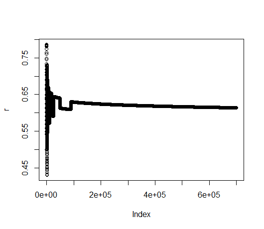
(a) MFG: $(\omega^{Q},\omega^{\mu})=(0.55,0.85)$

(b) MFG: $(\omega^{Q},\omega^{\mu})=(0.55,0.88)$

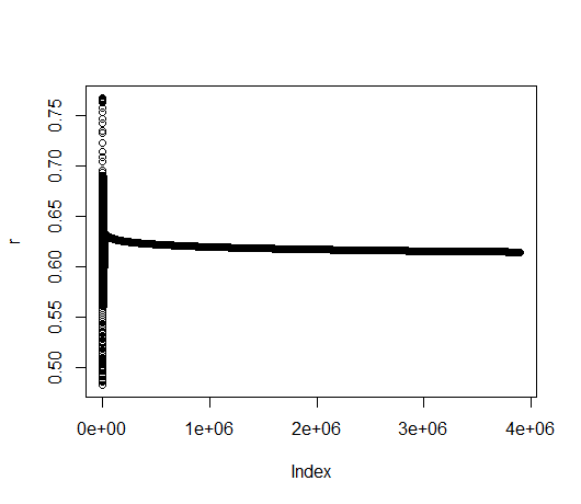
(c) MFG: $(\omega^{Q},\omega^{\mu})=(0.55,0.92)$

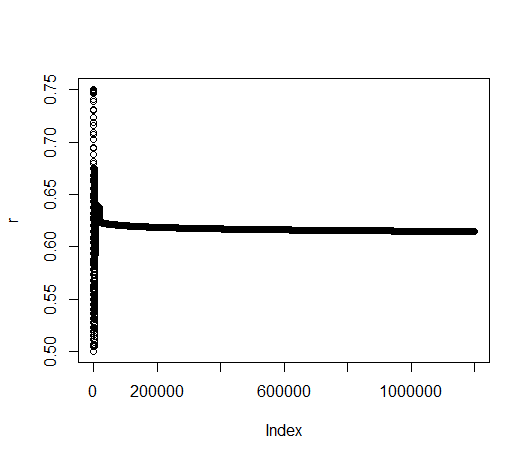
(d) MFG: $(\omega^{Q},\omega^{\mu})=(0.55,0.95)$

Figure 1: MFG setting: Convergence of the distribution. Each graph corresponds to one pair of $(\omega^{Q},\omega^{\mu})$, as indicated in the sub-caption. The plot represents the value of $\mu_{n}(x_{1})$ as a function of $n$.

The resulting distribution, which corresponds to the equilibrium distribution in the MFG scenario, is about $\mu=(\mu(x_{0}),\mu(x_{1}))=(0.386,0.614)$.

(a) $(\omega^{Q},\omega^{\mu})=(0.55,0.85)$

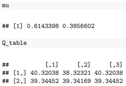
(b) $(\omega^{Q},\omega^{\mu})=(0.55,0.88)$

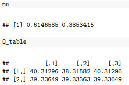
(c) $(\omega^{Q},\omega^{\mu})=(0.55,0.92)$

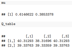
(d) $(\omega^{Q},\omega^{\mu})=(0.55,0.95)$

Figure 2: MFG setting: Limiting point. Each graph corresponds to one pair of $(\omega^{Q},\omega^{\mu})$, as indicated in the sub-caption. The plot represents the value of limiting point of $\mu_{n}$ and $Q_{n}$ as in the order of state $x_{1}$ and $x_{0}$.

5.2.2 MFC Experiment

In order to test the stability of different learning rates, the solution of MFC problem is reached based on the 4 choices $(\omega^{Q},\omega^{\mu})=(0.85,0.55),(0.88,0.55),(0.92,0.55),(0.95,0.55)$. These choices satisfy the assumptions that we used to prove convergence. Figure 3 illustrates the results. We provide the convergence plot of $\mu_{n}(x_{1})$, i.e., the value of the distribution at state 1, as a function of the step $n$. The y-axis is the value of $\mu_{n}(x_{1})$, and x-axis is number of iteration.

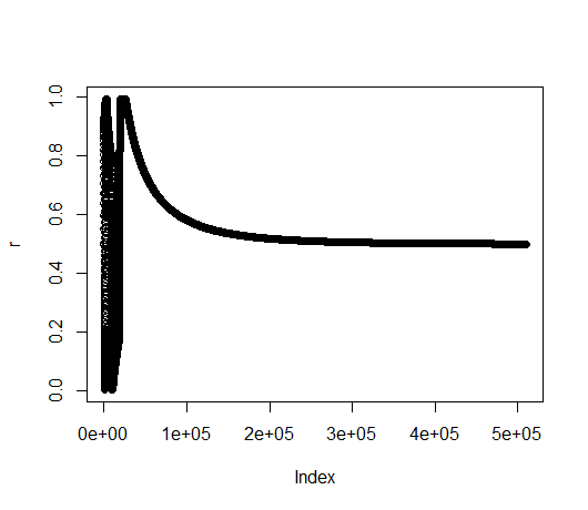
(a) MFC: $(\omega^{Q},\omega^{\mu})=(0.85,0.55)$

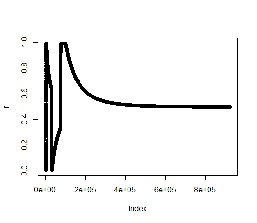
(b) MFC: $(\omega^{Q},\omega^{\mu})=(0.88,0.55)$

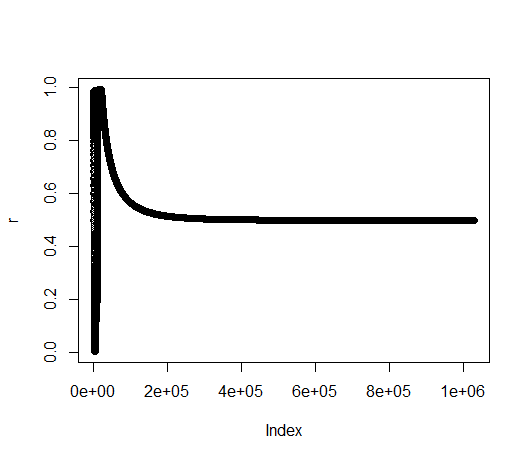
(c) MFC: $(\omega^{Q},\omega^{\mu})=(0.92,0.55)$

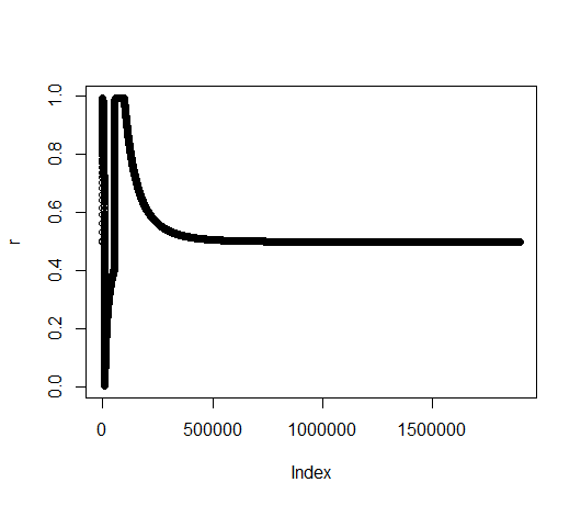
(d) MFC: $(\omega^{Q},\omega^{\mu})=(0.95,0.55)$

Figure 3: MFC setting: Convergence of the distribution. Each graph corresponds to one pair of $(\omega^{Q},\omega^{\mu})$, as indicated in the sub-caption. The plot represents the value of $\mu_{n}(x_{1})$ as a function of $n$.

The resulting distribution, which corresponds to the optimal distribution in the MFC scenario, is about $\mu=(\mu(x_{0}),\mu(x_{1}))=(0.5,0.5)$.

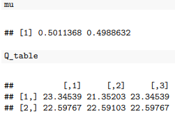
(a) $(\omega^{Q},\omega^{\mu})=(0.85,0.55)$

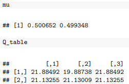
(b) $(\omega^{Q},\omega^{\mu})=(0.88,0.55)$

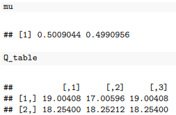
(c) $(\omega^{Q},\omega^{\mu})=(0.92,0.55)$

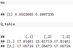
(d) $(\omega^{Q},\omega^{\mu})=(0.95,0.55)$

Figure 4: MFC setting: Limiting point. Each graph corresponds to one pair of $(\omega^{Q},\omega^{\mu})$, as indicated in the sub-caption. The plot represents the value of limiting point of $\mu_{n}$ and $Q_{n}$ as in the order of state $x_{1}$ and $x_{0}$.

5.2.3 Experiments with other choices of rates

Here we present numerical experiments with learning rates which do not satisfy the assumptions. This shows that the conditions used to prove convergence are simply sufficient conditions but in practice, the algorithm converges for a larger choice of learning rates.

We use constant learning rate for both MFG and MFC scenarios. For MFG, we take $(\rho^{Q},\rho^{\mu})=(0.01,0.0001)$. For MFC, we take $(\rho^{Q},\rho^{\mu})=(0.0001,0.01)$. As before, we provide the convergence plot of $\mu_{n}(x_{1})$, i.e., the value of the distribution at state 1, as a function of the step $n$. The y-axis is the value of $\mu_{n}(x_{1})$, and x-axis is number of iteration.

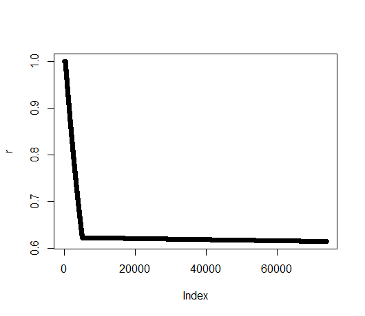
(a) MFG:constant learning rates $(\rho^{Q},\rho^{\mu})=(0.01,0.0001)$

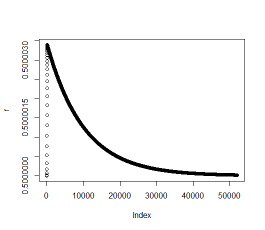
(b) MFC:constant learning rates $(\rho^{Q},\rho^{\mu})=(0.0001,0.01)$

The resulting distribution in the MFG scenario is about $\mu=(\mu(x_{0}),\mu(x_{1}))=(0.386,0.614)$, while in the MFC scenario, it is about $\mu=(\mu(x_{0}),\mu(x_{1}))=(0.5,0.5)$. This is consistent with the results presented above.

We also provide the limiting points for those constant learning rate under both MFG and MFC scenarios as 5

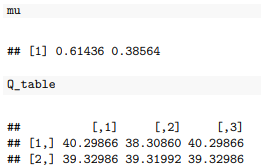
(c) MFG:constant learning rate

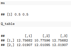
(d) MFC:constant learning rate

Figure 5: Limiting point for constant learning rate under MFG and MFC secarios.

6 Stochastic Approximation

In the previous section, we introduced an idealized deterministic algorithm relying on the operators $\mathcal{P}_{2}$ and $\mathcal{T}_{2}$, which involve expectations that we assumed we could compute perfectly. However, in more general case, those expectations are unknown and instead we use samples. Then we can use the theory of stochastic approximation to obtain convergence of algorithms with sample-based updates. In this section, we assume that the updates are still done in a synchronous way. The case of asynchronous updates is discussed in the next section.

In this section, we consider the following setting. Let us assume that for any $(\mu,x,a)$, the learner can know the value $f(x,a,\mu)$. Furthermore, the learner can sample a realization of the random variable

$$X^{{}^{\prime}}_{x,a,\mu}\sim p(\cdot|x,a,\mu),$$

Then, the learner has access to realizations of the following random variables $\widecheck{\mathcal{T}}_{\mu,Q}(x,a)$ and $\widecheck{\mathcal{P}}_{x,a,\mu}(\mu)$ taking values respectively in $\mathbbm{R}$ and $\Delta^{|\mathcal{X}|}$:

$$\begin{cases}\widecheck{\mathcal{T}}_{\mu,Q}(x,a)=f(x,a,\mu)+\gamma\min_{a^{\prime}}Q(X^{{}^{\prime}}_{x,a,\mu},a^{\prime})-Q(x,a)\\ (\widecheck{\mathcal{P}}_{x,a}(\mu)(x^{\prime}))_{x^{\prime}\in\mathcal{X}}=\left(\mathbbm{1}_{\{X^{{}^{\prime}}_{x,a,\mu}=x^{\prime}\}}-\mu(x^{\prime})\right)_{x^{\prime}\in\mathcal{X}}.\end{cases}$$

Observe that

$$\begin{cases}\mathbb{E}[\widecheck{\mathcal{T}}_{\mu,Q}(x,a)]=\sum_{x^{\prime\prime}}p(x^{\prime\prime}|x,a,\mu)\left[f(x,a,\mu)+\gamma\min_{a^{\prime}}Q(x^{\prime\prime},a^{\prime})-Q(x,a)\right]=\mathcal{T}_{2}(Q,\mu)(x,a)\\ \mathbb{E}[\widecheck{\mathcal{P}}_{x,a}(\mu)(x^{\prime})]=\sum_{x^{\prime\prime}}p(x^{\prime\prime}|x,a,\mu)(\mathbbm{1}_{\{x^{\prime\prime}=x^{\prime}\}}-\mu(x^{\prime}))=p(x^{\prime}|x,a,\mu)-\mu(x^{\prime}).\end{cases}$$

If the starting point $x$ comes from a random variable $X\sim\mu$ and if $a$ is an action chosen from a soft-min policy at $X$ according to $Q$, i.e., with probability distribution $\operatorname*{soft-min}Q(X,\cdot)$, then we obtain

$$\mathbb{E}[\widecheck{\mathcal{P}}_{X,\operatorname*{soft-min}Q(X)}(\mu)(x^{\prime})] =\sum_{x}\mu(x)\sum_{x^{\prime\prime}}p(x^{\prime\prime}|x,\operatorname*{soft-min}Q(x),\mu)(\mathbbm{1}_{\{x^{\prime\prime}=x^{\prime}\}}-\mu(x^{\prime}))$$

$$=\mathcal{P}_{2}(Q,\mu)(x^{\prime}).$$ (25)

Because of that, we can replace the deterministic updates by the following stochastic ones, starting from some initial $Q_{0}$, $\mu_{0}$: for $n=0,1,...,$

$$\begin{cases}\mu_{n+1}(x)&=\mu_{n}(x)+\rho^{\mu}_{n}\widecheck{\mathcal{P}}_{X_{n},\operatorname*{soft-min}Q(X_{n})}(\mu_{n})(x)\\ &=\mu_{n}(x)+\rho^{\mu}_{n}(\mathcal{P}_{2}(Q_{n},\mu_{n})(x)+\mathbf{P}_{n}(x)),\hskip 10.0pt\forall x\in\mathcal{X}\\ Q_{n+1}(x,a)&=Q_{n}(x,a)+\rho^{Q}_{n}\widecheck{\mathcal{T}}_{\mu_{n},Q_{n}}(x,a)\\ &=Q_{n}(x,a)+\rho^{Q}_{n}(\mathcal{T}_{2}(Q_{n},\mu_{n})(x,a)+\mathbf{T}_{n}(x,a)),\hskip 10.0pt\forall(x,a)\in\mathcal{X}\times\mathcal{A}\\ \hskip 30.0ptX_{n}&\sim\mu_{n}\end{cases}$$ (26)

where we introduced the notation:

$$\begin{cases}\mathbf{P}_{n}(x)=\widecheck{\mathcal{P}}_{X_{n},\operatorname*{soft-min}Q(X_{n})}(\mu_{n})(x)-\mathcal{P}_{2}(Q_{n},\mu_{n})(x)\\ \mathbf{T}_{n}(x,a)=\widecheck{\mathcal{T}}_{\mu_{n},Q_{n}}(x,a)-\mathcal{T}_{2}(Q_{n},\mu_{n})(x,a)\end{cases}$$ (27)

with $X_{n}$ sampled from $\mu_{n}$. Note that $\mathbf{T}_{n}$ and $\mathbf{P}_{n}$ are martingale difference sequences. Now we clearly define the system of iteration referring to [Borkar, 1997].

Next, we will establish the convergence of the two-timescale approach with stochastic approximation defined in (26).

Proposition 6.1.

Assume Assumptions 3.10 and Assumption 4.6 hold. Let $\psi^{\mu}_{n}(x):=\sum_{m=1}^{n}\rho^{\mu}_{m}\mathbf{P}_{m}(x)$ and $\psi^{Q}_{n}(x,a):=\sum_{m=1}^{n}\rho^{Q}_{m}\mathbf{T}_{m}(x,a)$. They are square integrable martingales and hence they converge as $n\to+\infty$.

Proof.

By Lemma 4.5 in [Borkar and Meyn, 2000], we directly have $\psi^{Q}_{n}$ is a square integrable martingale. Also we have $E[\|\mathbf{{P}}_{n}\|^{2}]<1$. Using this and the square summability of $\{\rho^{\mu}_{n}\}$ assumed in Assumption 3.10 and Assumption 4.6, the bound immediately follows, which shows that $\psi^{\mu}_{n}$ is also a square integrable martingale. Then by martingale convergence theorem [Neveu, 1975, p.62], we have the convergence of both martingales. ∎

For MFG, we have the following theorem.

Theorem 6.2.

Suppose Assumptions 3.10, 3.2, 3.6 and 3.7 hold. Then $(\mu_{n},Q_{n})_{n\geq 0}$ defined in (5) converges to $(\mu^{*\phi},Q^{*}_{\mu^{*\phi}})$ as $n\to\infty$.

Proof.

With Assumption 3.10, 3.2, 3.6 and 3.7, and the results of Propositions 3.3, 3.4, 3.5, 3.8, and 6.1, the assumptions of [Borkar, 1997, Theorem 1.1] are satisfied. This result guarantees the convergence in the statement. ∎

For MFC, we have the following theorem.

Theorem 6.3.

Suppose Assumptions 4.6, 3.2, 3.6 and 3.7 hold. Then $(\mu_{n},Q_{n})_{n\geq 0}$ defined in (5) converges to $(\mu^{*\phi}_{Q^{*\phi}},Q^{*\phi})$ as $n\to\infty$.

Proof.

With Assumptions 4.6, 3.2, 3.6, 3.7 and the results of Propositions 3.3, 3.4, 4.7, 4.8, and 6.1, the assumptions of [Borkar, 1997, Theorem 1.1] are satisfied. This result guarantees the convergence in the statement. ∎

7 Asynchronous Setting

In previous section, we assume that learner have access to a generative model, i.e., to a simulator which can provide the samples of transitions drawn according to the hidden dynamic for arbitrary state $x$. However a more realistic case is that the learner is constrained to follow the trajectory sampled by the environment without the ability to choose arbitrarily its state. We call this an asynchronous setting and the define the system as follows,

$$\mu_{n+1}=\mu_{n}+\rho_{n}^{\mu}(\mathcal{P}_{2}(Q_{n},\mu_{n})+\mathbf{P}_{n})$$ (28a)

$$Q_{n+1}(X_{n},A_{n})=Q_{n}(X_{n},A_{n})+\rho^{Q}_{n,X_{n},A_{n}}({\mathcal{T}_{2}}(Q_{n},{\mu}_{n})(X_{n},A_{n})+\mathbf{T}_{n}(X_{n},A_{n}))$$ (28b)

for $x\in\mathcal{X},\>a\in\mathcal{A},n\geq 0$, where $(X_{n},A_{n})$ is the state-action pair at time $n$. Comparing to the synchronous environment in the previous section, now we update the $Q$-table at one state-action pair for each time. As a consequence, the state-action pairs are not all visited at the frequency and the learning rate needs to be adjusted accordingly. We denote the learning rate for each state-action pair $(x,a)$ as $\rho^{Q}_{n,x,a}$. The martingale difference sequence is defined same as those in the previous section, namely (27).

Next, we will establish the convergence of the two-timescale approach with stochastic approximation under asynchronous setting defined in (28a)–(28b).

We will use the following assumption.

Assumption 7.1 (Ideal tapering stepsize (ITS)).

For any $(x,a)$, the sequence $(\rho^{Q}_{n,x,a})_{n\in\mathbbm{N}}$ satisfies the following conditions:

• (i) $\sum_{k}\rho^{Q}_{k,x,a}=\infty,$ and $\sum_{k}|\rho^{Q}_{k,x,a}|^{2}<\infty.$

• (ii) $\rho^{Q}_{k+1,x,a}\leq\rho^{Q}_{k,x,a}$ from some k onwards.

• (iii) there exists $r\in(0,1)$ such that $\sum_{k}(\rho^{Q}_{k,x,a})^{(1+q)}<\infty,\hskip 20.0pt\forall q\geq r.$

• (iv) for $\xi\in(0,1)$, $\sup_{k}\frac{\rho^{Q}_{[\xi k],x,a}}{\rho^{Q}_{k,x,a}}<\infty,$ where $[\cdot]$ stands for the integer part.

• (v) for $\xi\in(0,1)$, and $D(k):=\sum_{\ell=0}^{k}\rho^{Q}_{\ell,x,a}$, $\frac{D([yk])}{D(k)}\to 1,$ uniformly in $y\in[\xi,1]$.

With the asynchronous setting, we update step-by-step the Q table along the trajectory generated randomly. In order to ensure convergence, every state-action pair needs to be updated repeatedly. We introduce $\nu(x,a,n)=\sum_{m=0}^{n}\mathbbm{1}_{\{(X_{m},A_{m})=(x,a)\}}$ is the number of times the process $(X_{n},A_{n})$ visit state $(x,a)$ up to time $n$. The following assumptions are related to the (almost sure) good behavior of the number visits along trajectories.

Assumption 7.2.

There exists a deterministic $\Delta>0$ such that for all $(x,a)$,

$$\liminf_{n\to\infty}\frac{\nu(x,a,n)}{n}\geq\Delta\>\>\>\>\>a.s.$$

Furthermore, letting $N(n,\xi)=\min\left\{m>n:\sum_{k=n+1}^{m}\rho^{Q}_{k,x,a}>\xi\right\}$ for $\xi>0$, the limit

$$\lim_{n\to\infty}\frac{\sum_{k=\nu((x,a),n)}^{\nu((x,a),N(n,\xi))}\rho^{Q}_{k,x,a}}{\sum_{k=\nu((x^{\prime},a^{\prime}),n)}^{\nu((x^{\prime},a^{\prime}),N(n,\xi))}\rho^{Q}_{k,x^{\prime},a^{\prime}}}$$

exists a.s. for all pairs $(x,a)$, $(x^{\prime},a^{\prime})$.

Assumption 7.3.

There exists $d_{ij}>0$, such that for each $i=(x,a)$ and $j=(x^{\prime},a^{\prime})$

$$\lim_{n\to\infty}\frac{\sum_{m=0}^{n}\rho^{Q}_{m,j}}{\sum_{m=0}^{n}\rho^{Q}_{m,i}}=d_{ij}.$$

Proposition 7.4.

Suppose Assumptions 3.2, 3.6, and 3.7 hold. Then for every $\mu$, there exists a strict Lyapunov function for the function $Q\mapsto\mathcal{T}_{2}(Q,\mu)$. Likewise, there exists a strict Lyapunov function for the function $Q\mapsto\mathcal{T}_{2}(Q,{\mu^{*\phi}_{Q}})$.

Proof.

This is a direct consequence of the strict contraction property. For the first part, let us fix $\mu$. Recall from that $Q\mapsto\mathcal{B}_{\mu}Q$ is a strict contraction over $Q$ for any given $\mu$. Let $\tilde{Q}$ be defined by $\mathcal{T}_{2}(\tilde{Q},\mu)=0$. Let us define $V=\|Q-\tilde{Q}\|_{\infty}$. By [Borkar, 1998, Case 1, Page 844], $V$ is the strict Lyapunov function for $Q\mapsto\mathcal{T}_{2}(Q,\mu)$. For the second part, recall that $Q\mapsto\mathcal{B}_{\mu^{*\phi}_{Q}}Q$ is a strict contraction. So we can define $\tilde{Q}$ such that $\mathcal{T}_{2}(\tilde{Q},{\mu^{*\phi}_{\tilde{Q}}})=0$, and by [Borkar, 1998, Case 1, Page 844] $V=\|Q-\tilde{Q}\|_{\infty}$ is the corresponding strict Lyapunov function. ∎

For MFG, we have the following theorem.

Theorem 7.5.

Suppose Assumptions 3.10, 3.2, 3.6, 3.7, 7.1, 7.2 and 7.3 hold. Then, $(\mu_{n},Q_{n})_{n\geq 0}$ defined in (5) converges to $(\mu^{*\phi},Q^{*}_{\mu^{*\phi}})$ as $n\to\infty$.

Proof.

With Assumptions 3.10, 3.2, 3.6, 3.7, 7.1, 7.2, 7.3 and the results of Propositions 3.3, 3.4, 3.5, 3.8, 6.1 and 7.4, the assumptions of [Borkar, 1998, Theorem 3.1] and [Konda and Borkar, 1999, Lemma 4.11] are satisfied. This result guarantees the convergence in the statement. ∎

For MFC, we have the following theorem.

Theorem 7.6.

Suppose Assumptions 4.6, 3.2, 3.6, 3.7, 7.1, 7.2 and 7.3 hold. Then, $(\mu_{n},Q_{n})$ defined in (5) converges to $(\mu^{*\phi}_{Q^{*\phi}},Q^{*\phi})$ as $n\to\infty$.

Proof.

With Assumption 4.6, 3.2, 3.6, 3.7, 7.1, 7.2, 7.3 and the results of Propositions 3.3, 3.4, 4.7, 4.8, 6.1 and 7.4, the assumptions of [Borkar, 1998, Theorem 3.1] and [Konda and Borkar, 1999, Lemma 4.11] are satisfied. This result guarantees the convergence in the statement. ∎

8 MFCG Formulation and Three-timescale Approach

Following [Angiuli et al., 2022a], we now look at mixed mean field control games, which model competitive games between large numbers of large collaborative groups. The formulation takes place in discrete time and discrete space. The model involves the distribution of states within each collaborative groups (also called local distribution), and the distribution of states of the overall competitive population (also called global distribution).

The finite set of states is denoted by $\mathcal{X}$ and the finite set of actions that can be taken at each time step is denoted by $\mathcal{A}$. We denote by $\Delta^{|\mathcal{X}|}$ the simplex of probability measures on $\mathcal{X}$. Let $p_{3}$ : $\mathcal{X}\times\mathcal{X}\times\mathcal{A}\times\Delta^{|\mathcal{X}|}\times\Delta^{|\mathcal{X}|}\to\Delta^{|\mathcal{X}|}$ be a transition kernel and we assume this transition kernel depends on both the global distribution and the local distribution. We also interpret the kernel $p_{3}$ as a function

$$p_{3}:\mathcal{X}\times\mathcal{X}\times\mathcal{A}\times\Delta^{|\mathcal{X}|}\times\Delta^{|\mathcal{X}|}\to[0,1],\hskip 20.0pt(x,x^{\prime},a,\mu,\mu^{\prime})\mapsto p_{3}(x^{\prime}|x,a,\mu,\mu^{\prime})$$

which provides the probability that the process jumps to the states $x^{\prime}$ given the current state is $x$, the action $a$ is taken, the global distribution is $\mu$ and the local distribution is $\mu^{\prime}$. We allow for time homogeneous policies $\pi:\mathcal{X}\to\Delta^{|\mathcal{A}|}$ that depend on the state. We denote by $\mu^{\pi,\mu}$ the asymptotic local distribution of the controlled process following the strategy $\pi$ which we assume to exist and to be unique.

We go from finite horizon to infinite horizon so that the problem will be simpler to tackle with RL. Given a cost function $f$ defined on $\mathcal{X}\times\mathcal{A}\times\Delta^{|\mathcal{X}|}\times\Delta^{|\mathcal{X}|}$ and a discount rate $\gamma<1$, we now consider the following infinite horizon asymptotic mean field control game problem:

Definition 8.1.

A strategy $\hat{\pi}$, and a distribution $\hat{\mu}$ form a solution to the MFCG problem if:

1. (best response) $\hat{\pi}$ is the minimizer of

$$\pi\mapsto Q^{\pi}_{\hat{\mu}}=E\left[\sum_{n=0}^{\infty}\gamma^{n}f(X^{\pi,\hat{\mu}}_{n},\pi(X^{\pi,\hat{\mu}}_{n}),\hat{\mu},\mu^{\pi,\hat{\mu}})\right],$$

where $\mu^{\pi,\hat{\mu}}=\lim_{n\to\infty}\mathcal{L}(X^{\pi,\hat{\mu}}_{n})$ and $X^{\pi,\hat{\mu}}_{0}$ and

$$\begin{cases}X^{\pi,\hat{\mu}}_{0}\sim\mu_{0}\\ P(X^{\pi,\hat{\mu}}_{n+1}=x^{\prime}|X^{\pi,\hat{\mu}}_{n}=x,\pi(X^{\pi,\hat{\mu}}_{n})=a,\mu=\hat{\mu},\mu^{\prime}=\mu^{\pi,\hat{\mu}})=p_{3}(x^{\prime}|x,a,\hat{\mu},\mu^{\pi,\hat{\mu}}),\quad n\geq 0.\end{cases}$$

2. (consistency) $\hat{\mu}=\lim_{n\to\infty}\mathcal{L}(X^{\hat{\pi},\hat{\mu}}_{n})=\mu^{\hat{\pi},\hat{\mu}}$.

In order to make sense of the above problem statement we have to restrict to policies $\pi:\mathcal{X}\to\Delta^{|\mathcal{A}|}$ which are such that for any $\mu$ the controlled process $X^{\pi,\mu}_{n}$ has a limiting distribution, i.e. $\lim_{n\to\infty}\mathcal{L}(X^{\pi,\mu}_{n})$ exists. For a finite state Markov chain this is the case if $(X^{\pi,\mu}_{n})_{n}$ is irreducible and aperiodic. We therefore assume that the strategy $\hat{\pi}$ is the minimizer over all strategies such that $(X^{\pi,\hat{\mu}}_{n})_{n\in\mathcal{N}}$ is irreducible and aperiodic.

Algorithm 2 shows the pseudo-code for the Unified Three-timescale Mean Field Q-learning. For the learning rates, we recall that [Angiuli et al., 2022a] chose them of the following form

$$\rho^{Q}_{n,x,a}=\frac{1}{(1+\nu(x,a,n))^{\omega^{Q}}},\hskip 20.0pt\rho^{\mu}_{n}=\frac{1}{(1+(n+1))^{\omega^{\mu}}}\hskip 20.0pt\rho^{\tilde{\mu}}_{n}=\frac{1}{(1+(n+1))^{\omega^{\tilde{\mu}}}}$$

where $\omega^{Q}$, $\omega^{\mu}$ and $\omega^{\tilde{\mu}}$ are positive constants, and $\nu(x,a,n)=\sum_{m=0}^{n}\mathbbm{1}_{\{(X_{m},A_{m})=(x,a)\}}$ is the number of times the process $(X_{n},A_{n})$ visits state $(x,a)$ up to time $n$.

Algorithm 2 Unified Three-timescale Mean Field Q-learning

0:  $N_{steps}$: number of steps; $\phi$: parameter for $\operatorname*{soft-min}$ policy; $(\rho^{Q}_{n,x,a})_{n,x,a}$: learning rates for the value function; $(\rho^{\mu}_{n})_{n}$: learning rates for the global mean field; $(\rho^{\tilde{\mu}}_{n})_{n}$: learning rates for the local mean field

1:  Initialization: $Q_{0}(x,a)=0$ for all $(x,a)\in\mathcal{{X}}\times\mathcal{{A}}$, $\mu_{0}=[\frac{1}{|\mathcal{{X}}|},...,\frac{1}{|\mathcal{{X}}|}]$

2:  Observe $X_{0}$

3:  Update mean fields: $\mu_{0}=\tilde{\mu}_{0}=\boldsymbol{\delta}(X_{0})$

4:  for $n=0,1,2,\dots,N_{steps}-1$ do

5:     Choose action $A_{n}\sim\operatorname*{soft-min}_{\phi}Q_{n}(X_{n},\cdot)$ Observe cost $f_{n+1}=f(X_{n},A_{n},\mu_{n},\tilde{\mu}_{n})$ and state $X_{n+1}\sim p(\cdot|X_{n},A_{n},\mu_{n},\tilde{\mu}_{n})$ provided by the environment

6:     Update value function: $Q_{n+1}(x,a)=Q_{n}(x,a)$ for all $(x,a)\neq(X_{n},A_{n})$, and

$$Q_{n+1}(X_{n},A_{n})=Q_{n}(X_{n},A_{n})+\rho^{Q}_{n,X_{n},A_{n}}[f_{n+1}+\gamma\min_{a^{\prime}\in\mathcal{A}}Q_{n}(X_{n+1},a^{\prime})-Q_{n}(X_{n},A_{n})]$$

7:     Update mean fields: $\mu_{n+1}=\mu_{n}+\rho^{\mu}_{n}(\boldsymbol{\delta}(X_{n+1})-\mu_{n})$ and $\tilde{\mu}_{n+1}=\tilde{\mu}_{n}+\rho^{\tilde{\mu}}_{n}(\boldsymbol{\delta}(X_{n+1})-\tilde{\mu}_{n})$

8:  end for

9:  Return $(\mu_{N_{steps}},\tilde{\mu}_{N_{steps}},Q_{N_{steps}})$

8.1 Idealized Three-timescale Approach

To gain some intuition for the three-timescale approach used to approximate our MFCG, we start with the function $Q:\mathcal{X}\times\mathcal{A}\to\mathbbm{R}$ that describes the action values for some strategy $\pi^{\prime}$. Then at each time step when the system is at state $x$, the action $\arg\min_{a}Q(x,a)$ is chosen (assuming uniqueness). Say the global distribution $\mu$ is frozen and the local distribution is given by $\mu^{\pi,\mu}$, then the local population will in the next step be driven towards the new distribution $\mu^{\pi,\mu}P^{Q,\mu,\mu^{\pi,\mu}}$, if all players follow the strategy encoded in $Q$. This continues until a fixed-point $\mu^{\pi^{\prime},\mu}$ is reached. When a fixed-point is (approximately) reached, the strategy has to be updated, taking this new limiting distribution into account. This leads to a new strategy with action values given by

$$f(x,a,\mu,\mu^{\pi^{\prime},\mu})+\gamma\sum_{x^{\prime}}p(x^{\prime}|x,a,\mu,\mu^{\pi^{\prime},\mu})\min_{a^{\prime}}Q(x^{\prime},a^{\prime}).$$

This procedure continuous until, for the given global measure $\mu$, an optimal pair of strategy $\hat{\pi}$ and resulting limiting distribution measure $\mu^{\hat{\pi},\mu}$ is reached which depends on the frozen global measure $\mu$. In an outer global optimization the fixed-point for the global measure is now obtained by updating the global measure via $\mu P^{Q,\mu,\mu^{\hat{\pi},\mu}}$. The three time scales therefore arise naturally by the different layers of optimization involved in the problem. It is intuitive that in each layer one has to perform sufficiently many iterations to ensure that the optimization in the next layer is based on sufficiently accurate results. This idea leads to a learning rate that decreases from the outer to the inner layer. In addition the ratios of the increasing learning rates (from inner to outer layer) have to be sufficiently large.

These considerations lead to the following updating rules. For the sake of a lighter notation, we consider the triple $(\mu,Q,\mu^{\prime})$ where $\mu$ represents the global distribution and $\mu^{\prime}$ represents the local distribution. The triple is updated with rates $\rho^{\mu}_{n}<\rho^{Q}_{n}<\rho^{\mu^{\prime}}_{n}$ by

$$\begin{cases}\mu_{n+1}=\mu_{n}+\rho_{n}^{\mu}\mathcal{P}_{3}(\mu_{n},Q_{n},\mu^{\prime}_{n})\\ Q_{n+1}=Q_{n}+\rho^{Q}_{n}\mathcal{T}_{3}(\mu_{n},Q_{n},\mu^{\prime}_{n})\\ \mu^{\prime}_{n+1}=\mu^{\prime}_{n}+\rho_{n}^{\mu^{\prime}}\mathcal{P}_{3}^{\prime}(\mu_{n},Q_{n},\mu^{\prime}_{n})\end{cases}$$ (29)

where

$$\mathcal{P}_{3}(Q,\mu,\mu^{\prime})(x)=(\mu P^{Q,\mu,\mu^{\prime}})(x)-\mu(x)$$ (30a)

$$\mathcal{P}_{3}^{\prime}(Q,\mu,\mu^{\prime})(x)=(\mu^{\prime}P^{Q,\mu,\mu^{\prime}})(x)-\mu^{\prime}(x)$$ (30b)

$$P^{Q,\mu,\mu^{\prime}}(x,x^{\prime})=p(x^{\prime}|x,\operatorname*{soft-min}Q(x),\mu,\mu^{\prime})$$ (30c)

$$\mathcal{T}_{3}(\mu,Q,\mu^{\prime})(x,a)=f(x,a,\mu,\mu^{\prime})+\gamma\sum_{x^{\prime}}p(x^{\prime}|x,a,\mu,\mu^{\prime})\min_{a^{\prime}}Q(x^{\prime},a^{\prime})-Q(x,a)$$ (30d)

Now, following [Borkar, 1997], we consider the following ODE system which tracks the system (29):

$$\begin{cases}\dot{\mu}_{t}=\mathcal{P}_{3}(\mu_{t},Q_{t},\mu^{\prime}_{t})\\ \dot{Q}_{t}=\frac{1}{\epsilon}\mathcal{T}_{3}(\mu_{t},Q_{t},\mu^{\prime}_{t})\\ \dot{\mu^{\prime}_{t}}=\frac{1}{\epsilon\tilde{\epsilon}}\mathcal{P}_{3}^{\prime}(\mu_{t},Q_{t},\mu^{\prime}_{t}).\end{cases}$$ (31)

8.2 Convergence of Idealized Three-timescale Approach

In this section, we will establish the convergence of the idealized three-timescale approach defined in (29). In order to do it, let us introduce our additional assumptions:

Assumption 8.2.

The learning rate $\rho^{Q}_{n}$ and $\rho^{\mu}_{n}$ satisfy Assumption 3.10 and the learning rate $\rho^{Q}_{n}$ and $\rho^{\tilde{\mu}}_{n}$ satisfy Assumption 4.6.

Assumption 8.3.

The cost function $f$ is bounded and is Lipschitz with respect to $\mu$ and $\mu^{\prime}$, with Lipschitz constant denoted by $L_{f}^{glob}$ and $L_{f}^{loc}$ respectively, when using the $L^{1}$ norm. The transition kernel $p(\cdot|\cdot,\cdot,\mu,\mu^{\prime})$ is also Lipschitz with respect to $\mu$ and $\mu^{\prime}$, with Lipschitz constant denoted by $L_{p}^{glob}$ and $L_{p}^{loc}$ respectively, when using the $L^{1}$ norm. In other words, for every $x,a,\mu,\mu^{\prime}$, $\mu_{1}$, ${\mu^{\prime}_{1}}$

$$|f(x,a,\mu,\mu^{\prime})-f(x,a,\mu_{1},\mu^{\prime})| \leq L_{f}^{glob}\|\mu-\mu_{1}\|_{1}=L_{f}^{glob}\sum_{x}|\mu(x)-\mu_{1}(x)|,$$

$$|f(x,a,\mu,\mu^{\prime})-f(x,a,\mu,\mu^{\prime}_{1})| \leq L_{f}^{loc}\|\mu^{\prime}-\mu^{\prime}_{1}\|_{1}=L_{f}^{loc}\sum_{x}|\mu^{\prime}(x)-\mu^{\prime}_{1}(x)|,$$

$$\|p(\cdot|x,a,\mu,\mu^{\prime})-p(\cdot|x,a,\mu_{1},\mu^{\prime})\|_{1} \leq L_{p}^{glob}\|\mu-\mu_{1}\|_{1}=L_{p}^{glob}\sum_{x}|\mu(x)-\mu_{1}(x)|,$$

$$\|p(\cdot|x,a,\mu,\mu^{\prime})-p(\cdot|x,a,\mu,\mu^{\prime}_{1})\|_{1} \leq L_{p}^{loc}\|\mu^{\prime}-\mu^{\prime}_{1}\|_{1}=L_{p}^{loc}\sum_{x}|\mu^{\prime}(x)-\mu^{\prime}_{1}(x)|$$

Using Assumption 8.3, using a procedure similar to that of Proposition 3.3 and Proposition 3.4, we can show $(\mu,Q,\mu^{\prime})\mapsto\mathcal{P}_{3}(\mu,Q,\mu^{\prime})$ is Lipschitz over $\mu$ and $Q$, $(\mu,Q,\mu^{\prime})\mapsto\mathcal{P}^{\prime}_{3}(\mu,Q,\mu^{\prime})$ is Lipschitz over $\mu^{\prime}$ and $Q$, and $(\mu,Q,\mu^{\prime})\mapsto\mathcal{T}_{3}(\mu,Q,\mu^{\prime})$ is Lipschitz over $\mu$, $Q$ and $\mu^{\prime}$.

Remark 8.4.

On top of the above properties, $(\mu,Q,\mu^{\prime})\mapsto\mathcal{P}_{3}(\mu,Q,\mu^{\prime})$ is Lipschitz over $\mu^{\prime}$ and $(\mu,Q,\mu^{\prime})\mapsto\mathcal{P}^{\prime}_{3}(\mu,Q,\mu^{\prime})$ is Lipschitz over $\mu$ as well since:

$$\|\mathcal{P}_{3}(\mu,Q,\mu^{\prime})-\mathcal{P}_{3}(\mu,Q,\mu^{\prime}_{1})\|_{\infty} \leq\|\mathrm{P}^{\operatorname*{soft-min}_{\phi}Q,\mu,\mu^{\prime}}\mu-\mathrm{P}^{\operatorname*{soft-min}_{\phi}Q,\mu,\mu^{\prime}_{1}}\mu^{\prime}\|_{\infty}$$

$$\leq\|\mathrm{P}^{\operatorname*{soft-min}_{\phi}Q,\mu,\mu^{\prime}}\mu-\mathrm{P}^{\operatorname*{soft-min}_{\phi}Q,\mu,\mu^{\prime}_{1}}\mu)\|_{1}$$

$$\leq L_{p}^{loc}\|\mu^{\prime}-\mu^{\prime}_{1}\|_{1}.$$

Similarly, $\mathcal{P}_{3}^{\prime}$ is Lipschitz with respect to $\mu$.

Now that we have this Lipschitz property, we show that the O.D.E. system (29) has a unique global asymptotically stable equilibrium (GASE).

Assumption 8.5.

Let $L_{p}^{loc}+L_{p}^{glob}<|\mathcal{X}|c_{min}$.

Proposition 8.6.

Suppose Assumption 8.5 hold. For any given $Q$ and $\mu$, ${\dot{\mu^{\prime}_{t}}}=\mathcal{P}_{3}^{\prime}(\mu,Q,\mu^{\prime}_{t})$ has a unique GASE, that will denote by $\mu^{\prime*\phi}_{Q,\mu}$. Moreover, $\mu^{\prime*\phi}_{Q,\mu}:\mathbbm{R}^{|\mathcal{X}|\times|\mathcal{A}|}\to\Delta^{|\mathcal{X}|}$ is Lipschitz.

Proof.

Same as proof of Proposition 4.7. ∎

To prove that the GASE exists for the second and third O.D.E. in (29), we need to control the parameter $\phi$ properly to have a strict contraction so that we introduce the following assumption.

Assumption 8.7.

Assume $0<\phi<\min\left(\frac{|\mathcal{X}|c_{min}-L_{p}^{total}}{|\mathcal{A}|}\frac{1-\gamma}{L_{f}^{total}+\frac{\gamma}{1-\gamma}L_{p}^{total}\|f\|_{\infty}},\frac{(|\mathcal{X}|c_{min}-L_{p}^{glob})^{2}}{\phi|\mathcal{A}|(|\mathcal{X}|c_{min}-L_{p}^{glob}+L_{p}^{loc})}\frac{1-\gamma}{L_{f}^{glob}+\frac{\gamma}{1-\gamma}L_{p}^{glob}\|f\|_{\infty}}\right)$, where $L_{p}^{total}=L_{p}^{glob}+L_{p}^{loc}$ and $L_{f}^{total}=L_{f}^{glob}+L_{f}^{loc}$.

With this assumption, we have

$$\gamma+(L_{f}^{loc}+\gamma L_{p}^{loc}\|Q\|_{\infty})\frac{\phi|\mathcal{A}|}{|\mathcal{X}|c_{min}-L_{p}^{loc}}<1,$$

and

$$\frac{\phi|\mathcal{A}|(|\mathcal{X}|c_{min}-L_{p}^{glob}+L_{p}^{loc})}{|\mathcal{X}|c_{min}-L_{p}^{glob}}\frac{L_{f}^{glob}+\gamma L_{p}^{glob}\|Q^{*}_{\mu}\|_{\infty}}{1-\gamma}+L_{p}^{glob}+1-|\mathcal{X}|c_{min}<1,$$

which will give the strict contraction property we need in the next propositions.

Proposition 8.8.

Suppose Assumption 8.3 and 8.7 hold. Then for any given $\mu$, $\dot{Q}_{t}=\mathcal{T}_{3}(\mu,Q_{t},{\mu^{*\phi}_{Q_{t},\mu}})$ has a unique GASE, that we will denote by $Q^{*\phi}_{\mu}$.

The proof is omitted since it is similar to the proof of Proposition 4.8.

Proposition 8.9.

Under assumptions 8.3 and 8.7, $\dot{\mu}_{t}=\mathcal{P}_{3}(\mu_{t},Q^{*\phi}_{\mu_{t}},\mu^{\prime*\phi}_{Q^{*\phi}_{\mu_{t}},\mu_{t}})$ has a unique GASE, that we will denote by $\mu^{*\phi}$.

Proof.

We show that $\mu\mapsto\mathrm{P}^{\operatorname*{soft-min}_{\phi}Q^{*}_{\mu},\mu,\mu^{\prime*\phi}_{Q^{*\phi}_{\mu},\mu}}\mu$ is a strict contraction. We have (In short, we denote $\mu^{\prime*\phi}_{Q^{*\phi}_{\mu},\mu}$ as $\mu^{\prime}_{\mu}$):

$$\|\mathrm{P}^{\operatorname*{soft-min}_{\phi}Q^{*}_{\mu},\mu,\mu^{\prime}_{\mu}}\mu-\mathrm{P}^{\operatorname*{soft-min}_{\phi}Q^{*}_{\mu_{1}},\mu_{1},\mu^{\prime}_{\mu_{1}}}\mu_{1}\|_{1}$$

$$\leq|\mathrm{P}^{\operatorname*{soft-min}_{\phi}Q^{*}_{\mu},\mu,\mu^{\prime}_{\mu}}\mu-\mathrm{P}^{\operatorname*{soft-min}_{\phi}Q^{*}_{\mu^{\prime}},\mu,\mu^{\prime}_{\mu_{1}}}\mu\|_{1}+\|\mathrm{P}^{\operatorname*{soft-min}_{\phi}Q^{*}_{\mu},\mu,\mu^{\prime}_{\mu_{1}}}\mu-\mathrm{P}^{\operatorname*{soft-min}_{\phi}Q^{*}_{\mu_{1}},\mu,\mu^{\prime}_{\mu_{1}}}\mu\|_{1}$$

$$\hskip 14.22636pt+\|\mathrm{P}^{\operatorname*{soft-min}_{\phi}Q^{*}_{\mu_{1}},\mu,\mu^{\prime}_{\mu_{1}}}\mu-\mathrm{P}^{\operatorname*{soft-min}_{\phi}Q^{*}_{\mu_{1}},\mu_{1},\mu^{\prime}_{\mu_{1}}}\mu_{1}\|_{1}$$

$$\leq\|\mathcal{P}_{3}(\mu,Q^{*}_{\mu},\mu^{\prime}_{\mu})-\mathcal{P}_{3}(\mu,Q^{*}_{\mu},\mu^{\prime}_{\mu_{1}})\|_{1}+\|\mathcal{P}_{3}(\mu,Q^{*}_{\mu},\mu^{\prime}_{\mu_{1}})-\mathcal{P}_{3}(\mu,Q^{*}_{\mu_{1}},\mu^{\prime}_{\mu_{1}})\|_{1}$$

$$\qquad+\|\mathcal{P}_{3}(\mu,Q^{*}_{\mu},\mu^{\prime}_{\mu_{1}})-\mathcal{P}_{3}(\mu_{1},Q^{*}_{\mu_{1}},\mu^{\prime}_{\mu_{1}})\|_{1}$$

$$\leq L_{p}^{loc}\|\mu^{\prime}_{\mu}-\mu^{\prime}_{\mu_{1}}\|_{1}+\|\mathcal{P}_{3}(\mu,Q^{*}_{\mu},\mu^{\prime}_{\mu_{1}})-\mathcal{P}_{3}(\mu,Q^{*}_{\mu_{1}},\mu^{\prime}_{\mu_{1}})\|_{1}+(1+L_{p}^{glob}-|\mathcal{X}|c_{min})\|\mu-\mu_{1}\|_{1}$$

$$\leq\frac{L_{p}^{loc}\phi|\mathcal{A}|}{|\mathcal{X}|c_{min}-L_{p}^{glob}}\|Q^{*}_{\mu}-Q^{*}_{\mu_{1}}\|_{\infty}+\phi|\mathcal{A}|\|Q^{*}_{\mu}-Q^{*}_{\mu_{1}}\|_{\infty}+(1+L_{p}^{glob}-|\mathcal{X}|c_{min})\|\mu-\mu_{1}\|_{1}$$

$$\leq(\frac{\phi|\mathcal{A}|(|\mathcal{X}|c_{min}-L_{p}^{glob}+L_{p}^{loc})}{|\mathcal{X}|c_{min}-L_{p}^{glob}}\frac{L_{f}^{glob}+\gamma L_{p}^{glob}\|Q^{*}_{\mu}\|_{\infty}}{1-\gamma}+L_{p}^{glob}+1-|\mathcal{X}|c_{min})\|\mu-\mu_{1}\|_{1},$$

which shows the strict contraction property. As a result, by contraction mapping theorem [Sell, 1973], a unique GASE exists and furthermore by [Borkar and Soumyanatha, 1997, Theorem 3.1], $\mu_{t}$ will converge to it. ∎

Remark 8.10.

If we assume the existence of a unique GASE in Propositions 8.8 and 8.9, then we can omit the Assumption 8.7, which means that we can take any $\phi\geq 0$ without the upper bound. Moreover, we can also omit Assumption 8.7 in the following theorems.

Theorem 8.11.

Suppose Assumptions 8.2, 8.3, 8.5 and 8.7 hold. Then, $(\mu_{n},Q_{n},\mu^{\prime}_{n})$ defined in (29) converges to $(\mu^{*\phi},Q^{*\phi}_{\mu^{*\phi}},\mu^{\prime*\phi}_{Q^{*\phi}_{\mu^{*\phi}},\mu^{*\phi}})$ as $n\to\infty$.

Proof.

The arguments are similar so we only sketch the proof. With Assumption 8.2, 8.3, 8.5, 8.7 and the results of Propositions 3.3, 3.4, 8.6, 8.8 and 8.9, the assumptions of [Borkar, 1997, Theorem 1.1] are satisfied. This result guarantees the convergence in the statement. ∎

Next, we show that the limit point given by the algorithm, that is $(\mu^{*\phi},Q^{*\phi}_{\mu^{*\phi}},\mu^{\prime*\phi}_{Q^{*\phi}_{\mu^{*\phi}},\mu^{*\phi}})$, is an approximation of an MFCG solution in the sense of Definition 8.1. We denote $\alpha^{*\phi}_{\mu^{*\phi}}(x)=\arg\min_{a}Q^{*\phi}_{\mu^{*\phi}}(x,a)$ and $V^{*\infty}_{\mu^{*\phi}}(x)=Q^{*\phi}_{\mu^{*\phi}}(x,\alpha^{*\phi}(x))$. Then, we introduce the following assumption. We will denote $\mu^{{}^{\prime}*\phi}_{Q^{*\phi}_{\mu^{*\phi}},\mu^{*\phi}}$ as $\mu^{\prime*\phi}$ in the later proof.

Assumption 8.12.

There exists a unique solution to the Bellman equation (19) and there exist a $(\hat{\mu},\hat{Q},\hat{\mu}^{\prime})$ satisfying the following equation,

$$\begin{cases}\hat{\mu}^{\prime}=\mathrm{P}^{\arg\min\hat{Q},\hat{\mu},\hat{\mu}^{\prime}}\hat{\mu}^{\prime}\\ \hat{Q}=\mathcal{B}_{\hat{\mu},\hat{\mu}^{\prime}}\hat{Q},\\ \hat{\mu}=\mathrm{P}^{\arg\min\hat{Q},\hat{\mu},\hat{\mu}^{\prime}}\hat{\mu}\end{cases}$$ (32)

Remark 8.13.

By the unique GASE of $\mathcal{P}_{3}$ or $\mathcal{P}_{3}^{\prime}$, we will have $\mu^{*\phi}=\mu^{\prime*\phi}$ and $\hat{\mu}=\hat{\mu}^{\prime}$.

Theorem 8.14.

Suppose Assumptions 8.2, 8.3, 8.7 and 8.12. Let $(\hat{\mu},\hat{Q},\hat{\mu}^{\prime})$ be the solution of (32). Let $\delta$ be the action gap for $\hat{Q}$. Let $\phi=\frac{|\mathcal{X}|c_{min}-L_{p}^{total}}{|\mathcal{A}|}\frac{1-\gamma}{L_{f}^{total}+\frac{\gamma}{1-\gamma}L_{p}^{total}\|f\|_{\infty}}-\frac{1}{\delta}$. If $\phi>0$, then we have upper bounds as (33) below.

Proof.

We have:

$$\|\mu^{*\phi}-\hat{\mu}\|_{1} =\|\mathrm{P}^{\operatorname*{soft-min}_{\phi}Q^{*\phi}_{\mu^{*\phi}},\mu^{*\phi},\mu^{\prime*\phi}}\mu^{*\phi}-\mathrm{P}^{\arg\min\hat{Q},\hat{\mu},\hat{\mu}^{\prime}}\hat{\mu}\|_{1}$$

$$\leq\|\mathrm{P}^{\operatorname*{soft-min}_{\phi}Q^{*\phi}_{\mu^{*\phi}},\mu^{*\phi},\mu^{\prime*\phi}}\mu^{*\phi}-\mathrm{P}^{\operatorname*{soft-min}_{\phi}Q^{*\phi}_{\mu^{*\phi}},\mu^{*\phi},\hat{\mu}^{\prime}}\mu^{*\phi}\|_{1}$$

$$\hskip 14.22636pt+\|\mathrm{P}^{\operatorname*{soft-min}_{\phi}Q^{*\phi}_{\mu^{*\phi}},\mu^{*\phi},\hat{\mu}^{\prime}}\mu^{*\phi}-\mathrm{P}^{\operatorname*{soft-min}_{\phi}\hat{Q},\mu^{*\phi},\hat{\mu}^{\prime}}\mu^{*\phi}\|_{1}$$

$$\hskip 14.22636pt+\|\mathrm{P}^{\operatorname*{soft-min}_{\phi}\hat{Q},\mu^{*\phi},\hat{\mu}^{\prime}}\mu^{*\phi}-\mathrm{P}^{\arg\min\hat{Q},\mu^{*\phi},\hat{\mu}^{\prime}}\mu^{*\phi}\|_{1}+\|\mathrm{P}^{\arg\min\hat{Q},\mu^{*\phi},\hat{\mu}^{\prime}}\mu^{*\phi}-\mathrm{P}^{\arg\min\hat{Q},\hat{\mu},\hat{\mu}^{\prime}}\hat{\mu}\|_{1}$$

$$\leq L_{p}^{loc}\|\mu^{\prime*\phi}-\hat{\mu}^{\prime}\|_{1}+\phi|\mathcal{A}|\|Q^{*\phi}_{\mu^{*\phi}}-\hat{Q}\|_{\infty}+|\mathcal{A}|^{\frac{1}{2}}\max_{x\in\mathcal{X}}\|{\operatorname*{soft-min}}_{\phi}\hat{Q}(x)-\arg\min\hat{Q}(x)\|_{2}$$

$$\hskip 14.22636pt+(L_{p}^{glob}+1-|\mathcal{X}|c_{min})\|\mu^{*\phi}-\hat{\mu}\|_{1}$$

$$\leq L_{p}^{loc}\|\mu^{\prime*\phi}-\hat{\mu}^{\prime}\|_{1}+\phi|\mathcal{A}|\|Q^{*\phi}_{\mu^{*\phi}}-\hat{Q}\|_{\infty}+2|\mathcal{A}|^{\frac{3}{2}}\exp(-\phi\delta)$$

$$\hskip 14.22636pt+(L_{p}^{glob}+1-|\mathcal{X}|c_{min})\|\mu^{*\phi}-\hat{\mu}\|_{1}$$

$$\leq\phi|\mathcal{A}|\|Q^{*\phi}_{\mu^{*\phi}}-\hat{Q}\|_{\infty}+2|\mathcal{A}|^{\frac{3}{2}}\exp(-\phi\delta)+(L_{p}^{total}+1-|\mathcal{X}|c_{min})\|\mu^{*\phi}-\hat{\mu}\|_{1}$$

Also, we have the following

$$\|Q^{*\phi}_{\mu^{*\phi}}-\hat{Q}\|_{\infty} =\|\mathcal{B}_{\mu^{*\phi},\mu^{\prime*\phi}}Q^{*}_{\mu^{*\phi}}-\mathcal{B}_{\hat{\mu},\hat{\mu}^{\prime}}\hat{Q}\|_{\infty}$$

$$\leq\|\mathcal{B}_{\mu^{*\phi},\mu^{\prime*\phi}}Q^{*\phi}_{\mu^{*\phi}}-\mathcal{B}_{\mu^{*\phi},\hat{\mu}^{\prime}}Q^{*\phi}_{\mu^{*\phi}}\|_{\infty}+\|\mathcal{B}_{\mu^{*\phi},\hat{\mu}^{\prime}}Q^{*\phi}_{\mu^{*\phi}}-\mathcal{B}_{\hat{\mu},\hat{\mu}^{\prime}}Q^{*\phi}_{\mu^{*\phi}}\|_{\infty}$$

$$\hskip 14.22636pt+\|\mathcal{B}_{\hat{\mu},\hat{\mu}^{\prime}}Q^{*\phi}_{\mu^{*\phi}}-\mathcal{B}_{\hat{\mu},\hat{\mu}^{\prime}}\hat{Q}\|_{\infty}$$

$$\leq\gamma\|Q^{*\phi}_{\mu^{*\phi}}-\hat{Q}\|_{\infty}+(L_{f}^{glob}+\frac{\gamma}{1-\gamma}L_{p}^{glob}\|f\|_{\infty})\|\mu^{*\phi}-\hat{\mu}\|_{1}+(L_{f}^{loc}+\frac{\gamma}{1-\gamma}L_{p}^{loc}\|f\|_{\infty})\|\mu^{\prime*\phi}-\hat{\mu}\|_{1}$$

$$\leq\gamma\|Q^{*\phi}_{\mu^{*\phi}}-\hat{Q}\|_{\infty}+(L_{f}^{total}+\frac{\gamma}{1-\gamma}L_{p}^{total}\|f\|_{\infty})\|\mu^{*\phi}-\hat{\mu}\|_{1}.$$

So we have

$$((|\mathcal{X}|c_{min}-L_{p}^{total})-\frac{\phi|\mathcal{A}|(L_{f}^{total}+\frac{\gamma}{1-\gamma}L_{p}^{total}\|f\|_{\infty})}{1-\gamma})\|\mu^{*\phi}_{Q^{*\phi}}-\hat{\mu}\|_{1}\leq 2|\mathcal{A}|^{\frac{3}{2}}\exp(-\phi\delta).$$

Recall by Assumption 8.7, we have $((|\mathcal{X}|c_{min}-L_{p}^{total})-\frac{\phi|\mathcal{A}|(L_{f}^{total}+\frac{\gamma}{1-\gamma}L_{p}^{total}\|f\|_{\infty})}{1-\gamma})>0$, then we will have by taking $\phi=\frac{|\mathcal{X}|c_{min}-L_{p}^{total}}{|\mathcal{A}|}\frac{1-\gamma}{L_{f}^{total}+\frac{\gamma}{1-\gamma}L_{p}^{total}\|f\|_{\infty}}-\frac{1}{\delta}$,

$$\begin{cases}\|\mu^{*\phi}-\hat{\mu}\|_{1}=\|\mu^{\prime*\phi}-\hat{\mu}^{\prime}\|_{1}\leq\frac{2|\mathcal{A}|^{\frac{1}{2}}\delta(1-\gamma)}{(L_{f}^{total}+\frac{\gamma}{1-\gamma}L_{p}^{total}\|f\|_{\infty})}\exp(1-\frac{\delta(|\mathcal{X}|c_{min}-L_{p}^{total})}{|\mathcal{A}|}\frac{1-\gamma}{L_{f}^{total}+\frac{\gamma}{1-\gamma}L_{p}^{total}\|f\|_{\infty}})\\ \|Q^{*\phi}_{\mu^{*\phi}}-\hat{Q}\|_{\infty}\leq 2|\mathcal{A}|^{\frac{1}{2}}\delta\exp(1-\frac{\delta(|\mathcal{X}|c_{min}-L_{p}^{total})}{|\mathcal{A}|}\frac{1-\gamma}{L_{f}^{total}+\frac{\gamma}{1-\gamma}L_{p}^{total}\|f\|_{\infty}}).\end{cases}$$ (33)

Finally, we have for any $x\in\mathcal{X}$, $V^{*\phi}_{\mu^{*\phi}}(x)-\hat{V}(x)\leq\max(Q^{*\phi}_{\mu^{*\phi}}(x,\alpha^{*\phi}(x))-\hat{Q}(x,\alpha^{*\phi}(x)),Q^{*\phi}_{\mu^{*\phi}}(x,\hat{\alpha}(x))-\hat{Q}(x,\hat{\alpha}(x)))\leq\|Q^{*\phi}_{\mu^{*\phi}}-\hat{Q}\|_{\infty}$, so that $\|V^{*\phi}_{\mu^{*\phi}}-\hat{V}\|_{\infty}\leq\|Q^{*\phi}_{\mu^{*\phi}}-\hat{Q}\|_{\infty}$. ∎

8.3 Stochastic Approximation and Asynchronous Setting for Three time-scale System

Stochastic approximation for three time-scale system directly follows it for the two time-scale system, so that Theorem 6.2 and 6.3 still hold. In order to have the convergence for whole thee time-scale system, we need to follow both assumptions for Theorem 6.2 and 6.3. Furthermore, for the asynchronous setting, we can think the three time-scale system $(\mu,Q,\mu^{\prime})$ as two sub two-time-scale systems $(\mu,Q)$ and $(Q,\mu^{\prime})$. Both of these two time-scale system still can apply the Theorem 7.5 and 7.6 respectively. As a result, we can still have the convergence behaviour for three time-scale system under stochastic approximation and asynchronous setting.

9 Conclusion

In this paper, we first provide precise assumptions ensuring the convergence of the two-timescale RL algorithm proposed in [Angiuli et al., 2022b]. The proof relies on the theory of stochastic approximation. In order to use a contraction argument as in [Borkar, 1997], we smooth the strategies using a soft-min function characterized by one parameter which needs to be bounded by a quantity depending on the model parameters. Consequently, the algorithm may not convergence to the desired equilibrium solution but we provide a precise accuracy result of the approximation. One of the main properties of the algorithm is that it can approximate the solution of a Mean Field Game problem or of a Mean Field Control problem depending on the ratio of two learning rates. To illustrate this key fact, we give an example satisfying the sets of assumptions for the two problems. Finally, we extend our analysis to the case a three-timescale RL algorithm proposed in [Angiuli et al., 2022a] to solve competitive games between collaborative groups.

Appendix A Lipschitz property of the 2 scale operators

We define the $\operatorname*{soft-min}_{\phi}$ function in the following way:

$${\operatorname*{soft-min}}_{\phi}(z)=\left(\frac{e^{-\phi z_{i}}}{\sum_{j}e^{-\phi z_{j}}}\right)_{i=1,2,...,|\mathcal{A}|}$$ (34)

where $z\in\mathbbm{R}^{|\mathcal{A}|}$. By [Gao and Pavel, 2018], $\operatorname*{soft-min}_{\phi}$ is Lipschitz continuous for the $L^{2}$-norm and it is $\phi$-Lipschitz,

$$\|{\operatorname*{soft-min}}_{\phi}(z)-{\operatorname*{soft-min}}_{\phi}(z^{\prime})\|_{2}\leq\phi\|z-z^{\prime}\|_{2},\hskip 20.0ptz,z^{\prime}\in\mathbbm{R}^{|\mathcal{A}|}$$ (35)

Moreover, since $|\mathcal{A}|$ is finite, all the norms on $\mathbbm{R}^{|\mathcal{A}|}$ are equivalent, so that

$$\|{\operatorname*{soft-min}}_{\phi}(z)-{\operatorname*{soft-min}}_{\phi}(z^{\prime})\|_{1}\leq\phi\sqrt{|\mathcal{A}|}\|z-z^{\prime}\|_{1}$$ (36)

We also define an $\operatorname*{argmin-e}_{e}$ function in the following way:

$$\operatorname*{argmin-e}_{e}(z)_{i}=\begin{cases}\frac{1}{k}\hskip 28.45274pt\text{if }z_{i}=\min z\\ 0\hskip 28.45274pt\text{otherwise}\end{cases}$$

where $i=1,2,...,|\mathcal{A}|$. To be more clear, $\operatorname*{argmin-e}_{e}$ will assign equal to probability to the minimal value in $z$, and $0$ probability to others. Then We know that as $\phi\to 0$, the $\operatorname*{soft-min}_{\phi}$ function is smoother and smoother and the corresponding $L_{s}(\phi)\to 0$. On the opposite, the $\operatorname*{soft-min}_{\phi}$ will converge to $\operatorname*{argmin-e}_{e}$ as $\phi\to\infty$.

To alleviate the notation, we will write $Q(x):=(Q(x,a))_{a\in\mathcal{A}}$ for any $Q\in\mathbbm{R}^{|\mathcal{X}|\times|\mathcal{A}|}$, which implies $Q(x),\operatorname*{soft-min}_{\phi}Q(x),\operatorname*{argmin-e}_{e}Q(x)\in\mathbbm{R}^{|\mathcal{A}|}$. We also introduce a more general version transition kernel, which can take an input of a probability vector over actions instead of a single action: for $x,x^{\prime}\in\mathcal{X},\pi\in\Delta^{|\mathcal{A}|},\mu\in\Delta^{|\mathcal{X}|}$,

$$p(x^{\prime}|x,\pi,\mu)=\sum_{a}\pi(x)(a)p(x^{\prime}|x,a,\mu)$$ (37)

Also we introduce

$$f(x,\pi,\mu)=\sum_{a}\pi(x)(a)f(x,a,\mu)$$ (38)

References

• [Anahtarci et al., 2023] Anahtarci, B., Kariksiz, C. D., and Saldi, N. (2023). Q-learning in regularized mean-field games. Dynamic Games and Applications, 13(1):89–117.
• [Angiuli et al., 2022a] Angiuli, A., Detering, N., Fouque, J.-P., Laurière, M., and Lin, J. (2022a). Reinforcement learning algorithm for mixed mean field control games. arXiv:2205.02330.
• [Angiuli et al., 2023a] Angiuli, A., Fouque, J.-P., Hu, R., and Raydan, A. (2023a). Deep reinforcement learning for infinite horizon mean field problems in continuous spaces. arXiv preprint arXiv:2309.10953.
• [Angiuli et al., 2022b] Angiuli, A., Fouque, J.-P., and Laurière, M. (2022b). Unified reinforcement q-learning for mean field game and control problems. Mathematics of Control, Signals, and Systems, 34:217–271.
• [Angiuli et al., 2023b] Angiuli, A., Fouque, J.-P., and Laurière, M. (2023b). Reinforcement learning for mean field games, with applications to economics. Machine Learning and Data Sciences for Financial Markets: A Guide to Contemporary Practices, page 393.
• [Bensoussan et al., 2013] Bensoussan, A., Frehse, J., and Yam, S. C. P. (2013). Mean field games and mean field type control theory. Springer Briefs in Mathematics. Springer, New York.
• [Borkar and Soumyanatha, 1997] Borkar, V. and Soumyanatha, K. (1997). An analog scheme for fixed point computation. i. theory. IEEE Transactions on Circuits and Systems I: Fundamental Theory and Applications, 44(4):351–355.
• [Borkar, 1997] Borkar, V. S. (1997). Stochastic approximation with two time scales. Systems & Control Letters, 29(5):291–294.
• [Borkar, 1998] Borkar, V. S. (1998). Asynchronous stochastic approximations. SIAM Journal on Control and Optimization, 36(3):840–851.
• [Borkar and Meyn, 2000] Borkar, V. S. and Meyn, S. P. (2000). The o.d.e. method for convergence of stochastic approximation and reinforcement learning. SIAM Journal on Control and Optimization, 38(2):447–469.
• [Busoniu et al., 2008] Busoniu, L., Babuska, R., and De Schutter, B. (2008). A comprehensive survey of multiagent reinforcement learning. IEEE Transactions on Systems, Man, and Cybernetics, Part C (Applications and Reviews), 38(2):156–172.
• [Carmona and Delarue, 2018] Carmona, R. and Delarue, F. (2018). Probabilistic Theory of Mean Field Games with Applications I-II. Springer.
• [Carmona et al., 2019a] Carmona, R., Laurière, M., and Tan, Z. (2019a). Linear-quadratic mean-field reinforcement learning: Convergence of policy gradient methods. Preprint.
• [Carmona et al., 2019b] Carmona, R., Laurière, M., and Tan, Z. (2019b). Model-free mean-field reinforcement learning: Mean-field MDP and mean-field Q-learning. Preprint (To appear in the Annals of Applied Probability).
• [Cui and Koeppl, 2021] Cui, K. and Koeppl, H. (2021). Approximately solving mean field games via entropy-regularized deep reinforcement learning. In International Conference on Artificial Intelligence and Statistics, pages 1909–1917. PMLR.
• [Du et al., 2023a] Du, K., Jiang, Y., and Li, J. (2023a). Empirical approximation to invariant measures for mckean–vlasov processes: Mean-field interaction vs self-interaction. Bernoulli, 29(3):2492–2518.
• [Du et al., 2023b] Du, K., Jiang, Y., and Li, X. (2023b). Sequential propagation of chaos. arXiv preprint arXiv:2301.09913.
• [Du et al., 2023c] Du, K., Ren, Z., Suciu, F., and Wang, S. (2023c). Self-interacting approximation to mckean-vlasov long-time limit: a markov chain monte carlo method. arXiv preprint arXiv:2311.11428.
• [Elie et al., 2020] Elie, R., Perolat, J., Laurière, M., Geist, M., and Pietquin, O. (2020). On the convergence of model free learning in mean field games. In in proc. of AAAI.
• [Gao and Pavel, 2018] Gao, B. and Pavel, L. (2018). On the properties of the softmax function with application in game theory and reinforcement learning.
• [Gu et al., 2020] Gu, H., Guo, X., Wei, X., and Xu, R. (2020). Mean-field controls with q-learning for cooperative marl: Convergence and complexity analysis. arXiv preprint arXiv:2002.04131.
• [Gu et al., 2017] Gu, S., Holly, E., Lillicrap, T., and Levine, S. (2017). Deep reinforcement learning for robotic manipulation with asynchronous off-policy updates. In 2017 IEEE international conference on robotics and automation (ICRA), pages 3389–3396. IEEE.
• [Guo et al., 2019] Guo, X., Hu, A., Xu, R., and Zhang, J. (2019). Learning mean-field games. In Advances in Neural Information Processing Systems, pages 4966–4976.
• [Huang et al., 2006] Huang, M., Malhamé, R. P., and Caines, P. E. (2006). Large population stochastic dynamic games: closed-loop McKean-Vlasov systems and the Nash certainty equivalence principle. Commun. Inf. Syst., 6(3):221–251.
• [Konda and Borkar, 1999] Konda, V. R. and Borkar, V. S. (1999). Actor-critic–type learning algorithms for markov decision processes. SIAM Journal on Control and Optimization, 38(1):94–123.
• [Lanctot et al., 2017] Lanctot, M., Zambaldi, V., Gruslys, A., Lazaridou, A., Tuyls, K., Pérolat, J., Silver, D., and Graepel, T. (2017). A unified game-theoretic approach to multiagent reinforcement learning. Advances in neural information processing systems, 30.
• [Lasry and Lions, 2007] Lasry, J.-M. and Lions, P.-L. (2007). Mean field games. Jpn. J. Math., 2(1):229–260.
• [Laurière et al., 2022] Laurière, M., Perrin, S., Geist, M., and Pietquin, O. (2022). Learning mean field games: A survey. arXiv preprint arXiv:2205.12944.
• [Mguni et al., 2018] Mguni, D., Jennings, J., and de Cote, E. M. (2018). Decentralised learning in systems with many, many strategic agents. In Thirty-Second AAAI Conference on Artificial Intelligence.
• [Mnih et al., 2015] Mnih, V., Kavukcuoglu, K., Silver, D., Rusu, A. A., Veness, J., Bellemare, M. G., Graves, A., Riedmiller, M., Fidjeland, A. K., Ostrovski, G., et al. (2015). Human-level control through deep reinforcement learning. nature, 518(7540):529–533.
• [Neveu, 1975] Neveu, J. (1975). Discrete-parameter Martingales. North-Holland mathematical library. North-Holland.
• [Ouyang et al., 2022] Ouyang, L., Wu, J., Jiang, X., Almeida, D., Wainwright, C., Mishkin, P., Zhang, C., Agarwal, S., Slama, K., Ray, A., et al. (2022). Training language models to follow instructions with human feedback. Advances in Neural Information Processing Systems, 35:27730–27744.
• [Pasztor et al., 2021] Pasztor, B., Bogunovic, I., and Krause, A. (2021). Efficient model-based multi-agent mean-field reinforcement learning. arXiv preprint arXiv:2107.04050.
• [Perrin et al., 2020] Perrin, S., Pérolat, J., Laurière, M., Geist, M., Elie, R., and Pietquin, O. (2020). Fictitious Play for Mean Field Games: Continuous Time Analysis and Applications. In preparation.
• [Sell, 1973] Sell, G. R. (1973). Differential equations without uniqueness and classical topological dynamics. Journal of Differential Equations, 14(1):42–56.
• [Silver et al., 2016] Silver, D., Huang, A., Maddison, C. J., Guez, A., Sifre, L., Van Den Driessche, G., Schrittwieser, J., Antonoglou, I., Panneershelvam, V., Lanctot, M., et al. (2016). Mastering the game of go with deep neural networks and tree search. nature, 529(7587):484–489.
• [Subramanian and Mahajan, 2019] Subramanian, J. and Mahajan, A. (2019). Reinforcement learning in stationary mean-field games. In Proceedings. 18th International Conference on Autonomous Agents and Multiagent Systems.
• [Sutton and Barto, 2018] Sutton, R. S. and Barto, A. G. (2018). Reinforcement learning: An introduction. MIT press.
• [Vecerik et al., 2017] Vecerik, M., Hester, T., Scholz, J., Wang, F., Pietquin, O., Piot, B., Heess, N., Rothörl, T., Lampe, T., and Riedmiller, M. (2017). Leveraging demonstrations for deep reinforcement learning on robotics problems with sparse rewards. arXiv preprint arXiv:1707.08817.
• [Watkins, 1989] Watkins, C. J. C. H. (1989). Learning from delayed rewards. PhD thesis, King’s College, Cambridge.
• [Yang and Wang, 2020] Yang, Y. and Wang, J. (2020). An overview of multi-agent reinforcement learning from game theoretical perspective. arXiv preprint arXiv:2011.00583.
• [Zaman et al., 2023] Zaman, M. A. U., Koppel, A., Bhatt, S., and Basar, T. (2023). Oracle-free reinforcement learning in mean-field games along a single sample path. In International Conference on Artificial Intelligence and Statistics, pages 10178–10206. PMLR.
• [Zhang et al., 2021] Zhang, K., Yang, Z., and Başar, T. (2021). Multi-agent reinforcement learning: A selective overview of theories and algorithms. Handbook of reinforcement learning and control, pages 321–384.