Learning Robust Policies for Uncertain Parametric
Markov Decision Processes

Abstract

Synthesising verifiably correct controllers for dynamical systems is crucial for safety-critical problems. To achieve this, it is important to account for uncertainty in a robust manner, while at the same time it is often of interest to avoid being overly conservative with the view of achieving a better cost. We propose a method for verifiably safe policy synthesis for a class of finite state models, under the presence of structural uncertainty. In particular, we consider uncertain parametric Markov decision processes (upMDPs), a special class of Markov decision processes, with parameterised transition functions, where such parameters are drawn from a (potentially) unknown distribution. Our framework leverages recent advancements in the so-called scenario approach theory, where we represent the uncertainty by means of scenarios, and provide guarantees on synthesised policies satisfying probabilistic computation tree logic (PCTL) formulae. We consider several common benchmarks/problems and compare our work to recent developments for verifying upMDPs.

1 Introduction

Verifying the safety of complex dynamical systems is an important challenge (Knight, 2002), with applications including unmanned aerial vehicles (UAVs) (Yu and Dimarogonas, 2021) and robotics (Brunke et al., 2022). Ensuring a safety property may require verifying satisfaction of complex and rich formal specifications in the process of uncertainty arising from, for example, inaccurate modelling or process noise. A vital aspect of verification lies in finding abstractions that encompass this uncertainty, whilst accurately modelling system dynamics to aid optimal control of such systems.

In this paper we do not consider how such an abstraction may be generated and focus solely on learning a good controller/policy. There are a number of techniques for abstracting dynamical systems, such as the widely celebrated counter-example guided abstraction/refinement approach (Clarke et al., 2003). Alternatively, techniques make use of the so-called scenario approach in order to develop their models (Badings et al., 2023; Rickard et al., 2023).

One useful abstract model is that of parametric Markov decision processes (pMDPs) (Daws, 2004a; Hahn et al., 2011b; Junges et al., 2019), and particularly their probabilistic counterpart uncertain pMDPs (upMDPs) (Badings et al., 2022; Scheftelowitsch et al., 2017). Parametric MDPs extend MDPs by parameterising their transition function; any choice of parameters induces a standard MDP. Hence, a pMDP represents a family of MDPs, differing only in their transition function. By drawing these parameters from a (possibly unknown) distribution, we define an uncertain parametric MDP. The parameterisation of the model allows for the introduction of some structure, thus avoiding overly conservative models. Here, we make no assumptions on the structure of the parameterisation, and could equivalently have a direct distribution over MDPs within an uncertain set, hence arriving at a problem closely related to that of robust MDPs (Iyengar, 2005; Nilim and Ghaoui, 2005; Wiesemann et al., 2013).

A useful tool for expressing specifications on (up)MDPs lies in temporal logic (Platzer, 2012), a rich language for specifying behaviours of a system (Belta et al., 2017). One particular language of interest is that of Probabilistic Computation Tree Logic (PCTL (Hansson and Jonsson, 1994)), an extension of Computation Tree Logic which allows for probabilistic quantification of properties. This language can be used to describe probabilistic specifications on system behaviour, with these probabilities allowing for uncertainty. Often, it is of interest to learn a policy which ensures satisfaction of the specification (Hahn et al., 2011a), even under different realisations of the uncertainty.

One common approach for verifying pMDPs is to solve the so-called parameter synthesis problem, finding parameter sets that satisfy the specification. Typically, only a single set of parameters is of interest (Cubuktepe et al., 2022; Daws, 2004b; Meedeniya et al., 2014). Instead, we wish to synthesise policies that are probabilistically robust to uncertainty over the entire parameter space.

In this paper, we investigate the following problem. Given a upMDP, with a possibly unknown distribution over parameters, we aim at synthesising a policy, accompanied with a probabilistic certificate, such that, for an MDP defined with a randomly drawn parameter set, the probability that the policy satisfies a given specification on that MDP is guaranteed by the computed certificate. To solve this problem, we capitalize on advancements from the so-called scenario approach literature (Calafiore and Campi, 2006; Campi et al., 2009; Campi and Garatti, 2018; Garatti and Campi, 2022). We sample a finite number of parameter sets, and compute a policy that is robust to any sample within that set. Then, by leveraging results from Garatti and Campi (2022) we provide probably approximately correct (PAC) guarantees that the policy will be robust to a newly sampled parameter set. Importantly, these techniques allow us to provide guarantees based only on finite samples, without knowledge of the underlying distribution, and with no assumptions on the shape of this distribution or the geometry of its support set.

Since we are optimising a policy for multiple MDPs, our work is similar to developments on multiple environment MDPs (MEMDPs (Raskin and Sankur, 2014; van der Vegt et al., 2023)). These techniques consider finding policies which are optimal for a finite set of MDPs. In contrast to our approach, these methods assume to have complete knowledge of possible environments, whereas we wish to be robust to new, unseen, environments. Previous work in this area typically required overly conservative assumptions on the parameterisation, restricting to models where the uncertainty is independent across different states (Puggelli et al., 2013), or across different state-action pairs (Kozine and Utkin, 2002). In the robust MDP literature, such assumptions are referred to as $s$-rectangular or $(s,a)$-rectangular ambiguity sets (Wiesemann et al., 2013). Some recent approaches (Badings et al., 2022) have relaxed this assumption, but required full knowledge of the parameter sets at runtime in order to apply a policy.

Our work makes no assumption on the parameterisation of the upMDP, and learns a single policy which may be applied at runtime with no explicit parameter knowledge, whilst still offering PAC-type guarantees. Our main contributions can be summarised as follows

1. We formally discuss different policy classes for an MDP, and investigate their associated probabilistic guarantees. This policy classification is interesting per se as it clarifies subtle differences among them.

2. We propose a new gradient-based algorithm to learn an optimal robust policy for a given specification in an upMDP; we demonstrate the benefits of this scheme over more traditional solution paradigms via extensive numerical investigation and set the basis for a theoretical convergence analysis in future work;.

3. We use recent advancements of the scenario approach theory to accompany our synthesized policy with non-trivial guarantees on the probability that newly sampled MDPs will meet certain specifications.

2 Background

2.1 Markov Decision Processes

A Markov Decision Process (MDP) is a tuple $\mathcal{M}=(\mathcal{S},\mathcal{A},T,\rho,\gamma)$. Where $\mathcal{S}=\{s_{0},\dots,s_{N}\}$ is a finite set of states, with initial distribution $\rho:\mathcal{S}\rightarrow(0,1)$, $\mathcal{A}=\{a_{0},\dots,a_{M}\}$ a finite set of actions, $T\colon\mathcal{S}\times\mathcal{A}\rightarrow\Dist(\mathcal{S})$ is a probabilistic transition function, with $\Dist(\mathcal{S})$ the set of all probability distributions over $\mathcal{S}$ (Baier and Katoen, 2008), and $\gamma\in(0,1)$ is some discount factor.

We call a tuple $(s,a,s^{\prime})$ with probability $T(s,a)(s^{\prime})>0$ a transition. By absorbing state, we refer to a state $s\in\mathcal{S}$ in which all transitions return to that state with probability 1 so that $T(s,a)(s)=1$, for all $a\in\mathcal{A}$, these typically being some goal or critical states. An infinite trajectory of an MDP is a sampled sequence of states and actions $\zeta=s_{I}a_{0}s_{1}a_{1}\dots$, where actions are chosen according to some policy, which we define in the sequel.

2.1.1 Policy Classes

We consider three distinct classes of policy to determine actions in this MDP. Namely, deterministic (also called pure), mixed (also called randomized), and behavioural policies. These policies are denoted by $\pi^{D}\in\Pi^{D},\pi^{M}\in\Pi^{M},\pi^{B}\in\Pi^{B}$, referring to a deterministic, mixed and behavioural policy respectively. Specifically,

$$\pi^{D}\colon\mathcal{S}\rightarrow\mathcal{A},\hskip 56.9055pt\pi^{M}=\text{Dist}(\Pi^{D}),\hskip 56.9055pt\pi^{B}\colon\mathcal{S}\rightarrow\text{Dist}(\mathcal{A}).$$ (1)

In other words, a deterministic policy shows which action to pick at each state; a mixed policy provides directly a distribution over deterministic policies, so that we sample one policy at the start of a trajectory and follow it throughout; a behavioural policy gives us a distribution over actions at each state, so that we sample one action at each state of a trajectory. For MDPs, it can be shown that deterministic policies suffice for optimality, but this doesn’t hold for more complex models.

We denote by $\pi^{M}(\pi^{D})$ the probability of choosing $\pi^{D}$ under the distribution defined for the mixed policy, and by $\pi^{B}(s)(a)$ the probability of choosing action $a$ in a state $s$, under the policy defined by $\pi^{B}$. Mixed and behavioural policies offer two semantically different options to resolve the non-determinism in a probabilistic manner. For MDPs, there is a link between behavioural and mixed policies through Kuhn’s theorem (Arrow et al., 1953). Further, for an MDP, it is always possible to find memoryless behavioural policies that are realization-equivalent to mixed policies (see Appendix A for a proof). In Uncertain Parametric MDPs (introduced in the sequel) the link between behavioural and mixed policies may not be satisfied.

2.1.2 Uncertain Parametric MDP

An Uncertain Parametric MDP (upMDP) is a tuple $\mathcal{M}_{v}^{\mathbb{P}}=(\mathcal{S},\mathcal{A},\mathcal{V},\mathcal{T},\mathbb{P},\rho,\gamma)$. Similar to an MDP, but the probabilistic transition function is now $\mathcal{T}\colon\mathcal{S}\times\mathcal{A}\times\mathcal{V}\rightharpoonup\Dist(\mathcal{S})$, so that we denote by $\mathcal{T}_{v}(s,a)(s^{\prime})$ the probability of transitioning to state $s^{\prime}$, given action $a$ in $s$, with parameters $v\in\mathcal{V}$ (i.e. the transition function is parameterised by $v\in\mathcal{V}$), and with $\mathbb{P}$ defining a probability distribution over the parameter space. Thus, when a set of parameters $v$ is sampled, we extract a concrete MDP ${\mathcal{M}}[v]$. We do not impose any structure for this parameterisation, and only require that ${\mathcal{M}}[v]$ be a well-defined MDP. To uncover a trajectory in this upMDP we first sample a set of parameters $v$ from $\mathbb{P}$, and then follow a trajectory in the resulting MDP. We denote by $\mathbb{P}^{N}$ the product measure associated with $N$ sampled parameter sets.

2.2 Probabilistic Computation Tree Logic

Probabilistic computation tree logic (PCTL) depends on the following syntax:

$$\Phi::=\mathrm{true}\spacer p\spacer\neg\Phi\spacer\Phi\wedge\Phi\spacer\mathsf{P}_{\sim\lambda}(\psi)\hskip 56.9055pt\psi::=\Phi\,\mathsf{U}\,\Phi.$$ (2)

Here, $\sim\in\{<,\leq,\geq,>\}$ is a comparison operator and $\lambda\in[0,1]$ a probability threshold; PCTL formulae $\Phi$ are state formulae, which can in particular depend on path formulae $\psi$. Informally, the syntax consists of state labels $p\in AP$ in a set of atomic propositions $AP$, propositional operators negation $\neg$ and conjunction $\wedge$, and temporal operator until $\mathsf{U}$. The probabilistic operator $\mathsf{P}_{\sim\lambda}(\psi)$ requires that paths generated from the initial distribution satisfy a path formula $\psi$ with total probability exceeding (or below, depending on $\sim$) some given threshold $\lambda$. We consider only infinite horizon until, but note that extensions to include the finite time bounded-until operator can be achieved as discussed in Osband et al. (2019).

The satisfaction relation $\mathcal{M}[v]\sat_{\pi}\Phi$ defines whether a PCTL formula $\Phi$ holds true, when following policy $\pi$ in the concrete MDP. Formal definitions for semantics and model checking are provided in Hansson and Jonsson (1994); Baier and Katoen (2008).

2.2.1 PCTL Satisfaction

This satisfaction relation defines slightly semantics depending on the class of policy. We now explore these semantics for the policy classes identified in Section 2.1.1, namely, deterministic, mixed and behavioural, respectively.

$$\mathcal{M}\sat_{\pi^{D}}\mathsf{P}_{\geq\lambda}(\psi)\impliedby \sum_{\{\zeta\colon\zeta\sat\psi\}}\rho(s_{0})T(s_{1}\>|\>s_{0},\pi^{D}(s_{0}))T(s_{2}\>|\>s_{1},\pi^{D}(s_{1}))\dots\geq\lambda$$ (3)

$$=\sum_{\{\zeta\colon\zeta\sat\psi\}}P_{\pi^{D}}(\zeta)\geq\lambda,$$

$$\mathcal{M}\sat_{\pi^{M}}\mathsf{P}_{\geq\lambda}(\psi)\impliedby \sum_{\pi^{D}\in\Pi^{D}}\pi^{M}(\pi^{D})\cdot\left(\sum_{\{\zeta\colon\zeta\sat\psi\}}P_{\pi^{D}}(\zeta)\right)\geq\lambda,$$ (4)

$$\mathcal{M}\sat_{\pi^{B}}\mathsf{P}_{\geq\lambda}(\psi)\impliedby \sum_{\{\zeta\colon\zeta\sat\psi\}}\rho(s_{0})T(s_{1}\>|\>s_{0},a_{0})\pi^{B}(a_{0}\>|\>s_{0})T(s_{2}\>|\>s_{1},a_{1})\pi^{B}(a_{1}\>|\>s_{1})\dots\geq\lambda$$ (5)

$$=\sum_{\{\zeta\colon\zeta\sat\psi\}}P_{\pi^{B}}(\zeta)\geq\lambda.$$

We use the $P_{\pi}(\zeta)$ to refer to the probability of uncovering a trajectory when playing a given policy. Note that both eqs. 4 and 5 contain terms relating to the probability distributions introduced in the policy classes. Instead, eq. 3 only considers uncertainty in the model itself.

2.3 Robust Policies

We are interested in synthesising robust policies for upMDPs. That is, policies that maximise the probability of satisfying a PCTL formula $\psi$, within some given risk tolerance. Thus, we are interested in solving the chance-constrained optimisation program

$$\max_{\pi\in\Pi,~{}\lambda\in[0,1]}\lambda\hskip 19.91684pt\text{subject to }\hskip 8.5359pt\mathbb{P}\left\{v\in\mathcal{V}|\mathcal{M}[v]\sat_{\pi}\mathsf{P}_{\geq\lambda}(\psi)\right\}\geq 1-\epsilon.$$ (6)

for some a priori chosen risk level $\epsilon\in(0,1)$. There is an inherent tradeoff here between risk and satisfaction probability: namely, for a small risk we might obtain a small satisfaction probability, and vice versa. For brevity, we discuss only maximising $\lambda$, but note that the minimisation for $\sim\in\{<,\leq\}$ can be obtained trivially. Note that here we optimise over policies $\pi$ in a generic set $\Pi$; the exact policy class from the ones of Section 2.1.1 will be specified in the sequel.

3 Robust Policy Synthesis

Problem 1

Given an upMDP $\mathcal{M}_{v}^{\mathbb{P}}$, PCTL formula $\psi$ and risk level $\epsilon$, find a robust policy $\pi$ and maximum satisfaction probability $\lambda$, such that, with probability $1-\epsilon$ playing policy $\pi$ on a newly sampled MDP will satisfy the PCTL formula with satisfaction probability at least $\lambda$.

Due to the chance constraint on the parameter distribution $\mathbb{P}$, this problem is a semi-infinite optimization program (having a finite number of optimisation variables, but infinite constraints), and is generally intractable. Further, we may not have access to an analytical form for $\mathbb{P}$. Thus, we turn to a sample based analogue to this problem. In Section 4, we investigate how solutions to this problem can provide guarantees to the original chance-constrained problem.

Consider an upMDP $\mathcal{M}_{v}^{\mathbb{P}}$ and $N$ i.i.d. sampled parameter sets (or scenarios) $\mathcal{U}_{N}=\{u_{1},\dots,u_{N}\}$ sampled from $\mathbb{P}$. In this section, we investigate how to learn a robust policy which maximises the probability of satisfying a PCTL formula $\psi$, under the worst case realisation of the parameters, i.e. we investigate the following scenario program associated to eq. 6

$$\max_{\pi\in\Pi,~{}\lambda\geq 0}\lambda\hskip 28.45274pt\text{subject to }\text{sol}_{\mathcal{M}}^{\pi}(u;\psi)\geq\lambda,\;\forall u\in\mathcal{U}_{N}.$$ (7)

Where we use the notation $\text{sol}_{\mathcal{M}}^{\pi}(u;\psi)$ to refer to the maximum probability of satisfying a formula $\psi$, in the concrete MDP $\mathcal{M}[v]$, under policy $\pi$,

$$\text{sol}_{\mathcal{M}}^{\pi}(v;\psi)=\argmax_{\lambda\in[0,1]}\mathcal{M}[v]\sat_{\pi}\mathsf{P}_{\geq\lambda}(\psi).$$ (8)

This scenario program problem coincides closely with the concept of Multiple Environment MDPs (MEMDPs) (Raskin and Sankur, 2014), but differs in some key ways. When finding an optimal policy for MEMDPs, one wishes to find the policy that is optimal for the given environments. Instead, our goal to find a policy that will be robust to an unseen environment. Furthermore, the concrete chance constrained problem we study is drastically different to MEMDPs since it involves continuous parameters rather than a finite set of environments.

It is shown in Raskin and Sankur (2014) that infinite memory policies are required for optimality in MEMDPs. In our setting, infinite memory policies will indeed lead to optimal satisfaction probabilities in the sample set, but suffer when generalising to new samples. This can be seen as a problem of overfitting, and may also lead to a deterioration in our guarantees.

In the sequel, we provide different solution methodologies for eq. 7, where each methodology is based on a different class of policies.

3.1 Solution by Interval MDPs (under deterministic policies)

A straightforward approach to solve this problem is to ignore the structure induced by the parameterisation, and to build instead an interval MDP, where each transition is only known up to an interval. Each interval can be constructed by looking at each transition in turn and finding the minimum and maximum probabilities from the sampled MDPs. Such techniques are examined further (generally when no parameterisation is available) in Kozine and Utkin (2002) and are also closely aligned with the concept of $(s,a)$-rectangularity (Wiesemann et al., 2013). The resulting policy is in general very conservative, since it considers the worst case probability for every single transition. In reality, it is likely to be the case that the worst case transitions are unlikely to co-occur (for example, in a UAV motion planning problem like the one considered in Table 1 the wind may push us left or right into an obstacle, but is unlikely to do both).

3.2 MaxMin Game (under mixed policies)

The problem in eq. 7 can be rewritten as a MaxMin problem $\max_{\pi\in\Pi}\min_{u\in\mathcal{U}_{N}}\text{sol}_{\mathcal{M}}^{\pi}(u;\psi),$ which can be seen as a two player zero-sum game. In which we have a policy player, and the samples act as an adversary. The policy player’s actions are the set of all deterministic policies $\Pi^{D}$ for the upMDP, providing a finite, but potentially very large $\mathcal{O}(|\mathcal{A}|^{|\mathcal{S}|})$, action set. The sample adversary’s actions are the set of samples. Given sample $u$ and policy $\pi^{D}$, the reward to the policy player is $r_{p}(\pi^{D},u)=\text{sol}_{\mathcal{M}}^{\pi^{D}}(u;\psi)$. We may solve this as a Stackelberg game (Stackelberg, 1952; Yousefimanesh et al., 2023), with the adversary as the leader, to obtain an optimal deterministic policy. Details on this method, and associated results, are available in Appendix E.

Alternatively, a mixed strategy set $(s_{p},s_{\sigma})$, contains finite probability distributions over possible actions of each player, respectively, and returns the reward $r_{p}(s_{p},s_{\sigma})=\sum_{\pi^{D}\in\Pi^{D}}\sum_{u\in\mathcal{U}_{N}}s_{p}(\pi^{D})\cdot s_{\sigma}(u)\cdot\text{sol}_{\mathcal{M}}^{\pi_{D}}(u;\psi)$, or in matrix form $s_{p}Rs_{\sigma}$, where matrix $R\in\mathbb{R}^{|\Pi_{D}|\times N}$ has elements $R_{\pi_{D}^{i},u_{j}}=\text{sol}_{\mathcal{M}}^{\pi_{D}^{i}}(u_{j};\psi)$. Since the game consists of a finite number of players, each with a finite set of pure strategies, then by allowing players to play mixed strategies, it can be shown that a Nash equilibrium of the game will exist, and further, that all Nash equilibria have the same value. Note that the mixed strategy defines a mixed policy $s_{p}=\pi^{M}$.

Theorem 3.1 (Nash Equilibrium Nash (1989); Frihauf et al. (2012)).

For a two player zero-sum game, there exists at least one mixed strategy profile $s^{\star}=(s^{\star}_{p},s^{\star}_{\sigma})$, such that

$$r_{p}(s^{\star}_{p},s^{\star}_{\sigma})\geq r_{p}(s_{p},s^{\star}_{\sigma}),\forall s_{p}\in S_{p},\hskip 28.45274ptr_{p}(s^{\star}_{p},s^{\star}_{\sigma})\leq r_{p}(s^{\star}_{p},s_{\sigma}),\forall s_{\sigma}\in S_{\sigma}.$$ (9)

If both inequalities are strict, then there is a single unique Nash equilibrium, called a strict Nash equilibrium. Otherwise, there is a set of Nash equilibria, all having equal value.

Finding Nash equilibrium strategies in this game is relatively straightforward, and there are a number of existing methods for solving the game (for example, the Porter-Nudelman-Shoham (PNS) algorithm (Porter et al., 2008, Algorithm 1) or fictitious play methods (Heinrich et al., 2015)). Thus, we can simply build the reward matrix $R$, by considering each determinsitic policy and sample in turn, and pass this to one of these algorithms. Unfortunately, this method is computationally very expensive, with the size of the reward matrix being $\mathbb{R}^{N\times|\mathcal{S}|^{|\mathcal{A}|}}$, and algorithms to solve such games being exponential in the size of this matrix.

3.3 Subgradient Ascent (under behavioural policies)

Under the choice of behavioural policies, we propose an alternative method that avoids computing a full payoff matrix for every deterministic policy. Taking inspiration from Bhandari and Russo (2019), we rewrite the solution function as $\text{sol}_{\mathcal{M}}^{\pi^{B}}(u;\psi)=\sum_{s\in\mathcal{S}}\eta^{u}_{\pi^{B}}(s)\sum_{a\in\mathcal{A}}Q^{u}_{\pi^{B}}(s,a)\pi^{B}(s)(a),$ where $Q^{u}_{\pi^{B}}(s,a)$ is a Q-function, defined to model the PCTL requirement (see Appendix B) and $\eta^{u}_{\pi^{B}}(s)$ is the discounted state-occupancy measure $\eta^{u}_{\pi^{B}}(s)=(1-\gamma)\sum_{k=0}^{\infty}\gamma_{k}P^{\pi^{B}}_{k}(s)$, with $P^{\pi^{B}}_{k}(s)$ the probability of uncovering state $s$ at time $k$. Intuitively, $\eta^{u}_{\pi^{B}}(s)$ defines the (discounted) fraction of time the system spends in a given state. We fix $\eta^{u}_{\pi^{B}}$ and $Q^{u}_{\pi^{B}}$ (as in policy iteration (Foster, 1962)), and find the gradient (given analytically in Section 3.3).

This provides us with a (sub)gradient for a single solution function, however, we are primarily interested in the pointwise minimum amongst a set of solution functions. Hence, we turn to subdifferentials (or subgradients) (Kiwiel, 2001; Aussel et al., 1995). One simple way of finding a valid subdifferential is to find the gradient of one of the current minimum functions.

Projected Subgradient Ascent upMDP $\mathcal{M}$, samples $\mathcal{U}_{N}$, formula $\psi$, step-size sequence $\{\alpha_{0},\alpha_{1},\dots\}$ Optimal Policy $\pi$ $k\leftarrow 0$  $\pi^{B}_{0}\leftarrow\text{uniform random}$
not converged $u^{\star}\leftarrow\text{random choice}(\argmin_{u\in\mathcal{U}_{N}}\text{sol}_{\mathcal{M}}^{\pi^{B}_{k}}(u;\psi))$ Select worst case sample $\nabla_{k+1}(s,a)=\sum_{s\in\mathcal{S}}\eta^{u^{\star}}_{\pi^{B}}(s)\sum_{a\in\mathcal{A}}Q^{u^{\star}}_{\pi^{B}}(s,a)$ Find gradient for worst case $\pi^{B}_{k+1}(s)(a)\leftarrow\text{proj}_{\sum\pi^{B}(\cdot\>|\>s)=1}[\pi^{B}_{k}+\alpha_{k}\nabla_{k+1}(s,a)]$ Gradient step $f^{k+1}_{\ast}=\max\{f^{k}_{\ast},f(\pi^{B}_{k+1})\}$ Store record objective $k\leftarrow k+1$
We initialise with a uniform random policy, select a minimising (worst-case) sample from the set of minimisers (which may not be a singleton), then find the gradient for this sample, take a step in this direction, and project onto the constraint set. We use a diminishing, non-summable step size $\alpha_{k}$, typically employed in subgradient methods. We give numerical evidence that this algorithm exhibits a convergent behaviour in Section 5, and further analysis in Appendix D.

4 Guarantees

Once we have synthesised a policy using one of the methods above, we can accompany each of the policies synthesized according to the aforementioned methodologies with PAC-type guarantees on the satisfaction of the PCTL property under consideration. To achieve this, we use the following recent result in the scenario approach theory.

Given the solution to a scenario program, we are interested in quantifying the risk associated with the solution (i.e. the probability that our solution violates a new sampled constraint). The scenario approach provides us with the techniques to achieve this by considering the number of support constraints. In an optimisation problem, if the removal of a constraint leads to a changed solution, then this constraint is said to be a support constraint. Further, if a solution returned when considering only the support constraints is the same as the solution obtained when employing all samples, then the problem is a non-degenerate problem.

Theorem 4.1 (PAC Guarantees Garatti and Campi (2022)).

Consider the optimisation problem in eq. 7, with $N$ sampled parameter sets. Given a confidence parameter $\beta\in(0,1)$, for any $k=0,1,\dots,N$, consider the polynomial equation in the variable $t$

$$\xi_{k}(t)=\begin{cases}1-\frac{\beta}{6N}\sum_{i=N+1}^{4N}\binom{i}{k}t^{i-k},&\text{if }k=N,\\ \binom{N}{k}t^{N-K}-\frac{\beta}{2N}\sum_{i=k}^{N-1}\binom{i}{k}t^{i-k}-\frac{\beta}{6N}\sum_{i=N+1}^{4N}\binom{i}{k}t^{i-k},&\text{otherwise.}\\ \end{cases}$$ (10)

Solving $\xi_{k}(t)=0$ for $t\in[0,+\infty)$, for $k=0,1,\dots,N-1$, we find exactly two solutions, which we denote with $\underline{t}(k),\overline{t}(k)$ with $\underline{t}(k)\leq\overline{t}(k)$. For $k=N$, we find a single solution, which we denote by $\overline{t}(N)$, and define $\underline{t}(N)=0$. Let $\underline{\epsilon}(k)\coloneqq\max\{0,1-\overline{t}(k)\}$ and $\overline{\epsilon}(k)\coloneqq 1-\underline{t}(k)$.

Assume the problem is non-degenerate, and has a unique solution. Let $\pi_{N}^{\ast}$ be the optimal policy, $\lambda_{N}^{\ast}$ the optimal satisfaction probability, and $\tilde{s}^{\ast}_{N}$ is the number of support samples. Then, for any $\mathbb{P}$ it holds that

$$\mathbb{P}^{N}\{\underline{\epsilon}(\tilde{s}^{\ast}_{N})\leq\mathbb{P}\left\{v\in\mathcal{V}\colon\mathcal{M}[v]\notsat_{\pi^{M}}\mathsf{P}_{\geq\lambda^{\star}}(\psi)\right\}\leq\overline{\epsilon}(\tilde{s}^{\ast}_{N})\}\geq 1-\beta,$$ (11)

where $\mathbb{P}\left\{v\in\mathcal{V}\colon\mathcal{M}[v]\notsat_{\pi^{M}}\mathsf{P}_{\geq\lambda^{\star}}(\psi)\right\}$ is the risk (the probability that our solution violates the specification for another sample $v$).

Note that in $\pi_{N}^{\ast}$ we do not specify the problem class; this is considered in the sequel when we deploy this theorem for each solution methodology from the previous section. Moreover, to determine the number of support samples $\tilde{s}^{\ast}_{N}$, we exploit our problem’s structure and, based on the solution methodology adopted, we discuss how an upper-bound on their number can be obtained.

To this end, we provide guarantees for the policy generated by each of the methods of Section 3. Consider first the case of the mixed policy determined using a Nash equilibrium solver as per the developments of Section 3.2. In this case, finding the number of support samples consists of finding samples which are included in the mixed strategy of the sampled adversary.

Corollary 4.2 (PAC Guarantees for Mixed Policies).

Consider the MaxMin game of Section 3.2, and let $\pi_{N}^{\ast}$ be the optimal mixed policy $\pi^{M}$ returned by a Nash equilibrium solver. The number of support constraints may be found as $\tilde{s}^{\ast}_{N}=|\{u\in\mathcal{U}_{N}\colon s_{\sigma}(u)>0\}|$, while the satisfaction relation $\mathcal{M}[v]\notsat_{\pi^{M}}\mathsf{P}_{\geq\lambda^{\star}}(\psi)$ is as defined in eq. 4.

Consider now the case of a behavioural policy obtained using the subgradient methodology (Section 3.3). We determine the number of support constraints by finding the active constraints (as the problem is assumed to be non-degenerate, the active constraints are also the support constraints).

Corollary 4.3 (PAC Guarantees for Behavioural Policies).

Consider the subgradient algorithm of Section 3.2, and let $\pi_{N}^{\ast}$ be the optimal behavioural policy $\pi^{B}$ returned by Algorithm 3.3. The number of support samples is given by the active constraints, which are in turn the ones for which the obtained satisfaction probability $\lambda^{\star}$ is tight, i.e., $\tilde{s}^{\ast}_{N}=|\{u\in\mathcal{U}_{N}\colon\text{sol}_{\mathcal{M}}^{\pi^{B}}(u;\psi)=\lambda^{\star}\}|,$ while the satisfaction relation $\mathcal{M}[v]\notsat_{\pi^{B}}\mathsf{P}_{\geq\lambda^{\star}}(\psi)$ is as defined in eq. 5.

Finally, consider the construction of an interval MDP under the class of deterministic policies. In this case, our problem is degenerate, since it may be necessary to remove multiple constraints for another policy to become optimal, thus prohibiting the use of Theorem 2. Therefore, we leverage techniques from Campi et al. (2018) that do not require imposing a non-degeneracy assumption.

Corollary 4.4 (PAC Guarantees for iMDP Policies).

Fix $\beta\in(0,1)$, and as in (Campi et al., 2018, Theorem 1), define $\mu(N)\coloneqq 1$, and for $\tilde{s}^{\ast}_{N}<N$ let

$$\mu(\tilde{s}^{\ast}_{N})\coloneqq 1-\sqrt[N-\tilde{s}^{\ast}_{N}]{\frac{\beta}{N\binom{N}{\tilde{s}^{\ast}_{N}}}}.$$ (12)

Support samples are those which define the intervals: $\overline{\tilde{s}^{\ast}_{N}}=|\{u\in\mathcal{U}_{N}\colon\exists(s,a,s^{\prime}),T_{u}(s,a)(s^{\prime})\leq T_{v}(s,a)(s^{\prime})\vee T_{u}(s,a)(s^{\prime})\geq T_{v}(s,a)(s^{\prime}),\forall v\in\mathcal{U}_{N}\}|,$ i.e., those with at least one transition probability at an extremum of its interval. Then (with satisfaction relation defined in eq. 3) we have

$$\mathbb{P}^{N}\left\{\mathbb{P}\left\{v\in\mathcal{V}\colon\mathcal{M}[v]\notsat_{\pi^{D}}\mathsf{P}_{\geq\lambda^{\star}}(\psi)\right\}\leq\mu(\overline{\tilde{s}^{\ast}_{N}})\right\}\geq 1-\beta.$$ (13)

5 Numerical Experiments

We implemented our techniques in Python and made use of the probabilistic model checker Storm (Hensel et al., 2022) to verify PCTL formulae on MDPS, and PRISM (Kwiatkowska et al., 2011) for iMDPs. Experiments were run on a server with 80 2.5 GHz CPUs and 125 GB of RAM. The codebase is available at https://github.com/lukearcus/robust_upMDPhttps://github.com/lukearcus/robust_upMDP

We evaluate our techniques on a number of benchmark models available in the literature (Quatmann et al., 2016), as well as a few simpler examples, for a complete description see Appendix C. We compare our subgradient algorithm (Section 3.3) to existing techniques from Badings et al. (2022) (column 1) and an implementation of the synthesis based on iMDP, as in Kozine and Utkin (2002) (column 2). Unless otherwise stated, we use a numerical tolerance of $10^{-4}$, a confidence parameter of $\beta=10^{-5}$, take $N=200$ parameter samples, and allow 1 hour of computation time. We provide numerical values for the optimal satisfaction probability $\lambda^{\star}$, the theoretical risk upper bound $\overline{\epsilon}$, the runtimes, the empirical values of the risk $\tilde{\epsilon}$, and the empirical values of the risk without access to the true parameter set (if parameter access is needed to synthesise a policy, we draw a sample $v_{1}\sim\mathbb{P}$ for synthesis, but test on sample, $v_{2}\sim\mathbb{P}$). We highlight in grey cases where we discuss next how the methodologies under comparison are compared/outperformed by our proposed subgradient algorithm either in terms of the quality of their probabilistic guarantees and/or the computational requirements, and use red text for empirical values which violate a bound.

Our subgradient algorithm is less conservative than a naive iMDP solution, offering non-trivial theoretical risk bounds (for the iMDP approach these bounds are often equal to one), and superior satisfaction probabilities (the iMDP approach considers the worst case probability for every transition). By superior, we mean either higher or lower depending on the optimisation direction (maximisation or minimisation, respectively, denoted by (max) and (min) in Table 1). The approach in Badings et al. (2022) generally outperforms our methods in speed, risk bounds and satisfaction probability. The difference on the theoretical risk bounds lies in the fact that our approach involves solving a problem with a non-trivial number of support constraints, while in Badings et al. (2022) they have only one support constraint. As such, it offers tighter guarantees, however, these refer to an existential statement. To see this, note that Badings et al. (2022) compute a different policy per sample, and provide guarantees only on the existence of a policy for a new sample. On the contrary, we construct a policy that is robust with respect to all samples, and at the same time is accompanied by guarantees on its feasibility properties for unseen samples. Moreover, Badings et al. (2022) require access to true parameters at runtime, and a non-trivial amount of online computation to solve the MDP. Without this, their risk bounds may be violated (as seen in red).

Our mixed policy solution (Section 3.2), timed out on all but the toy model, for which the results are: Sat. Prob: .325, Risk U.B.: .147, runtime: 0.75s Emp. risk: .003, Emp. risk (no pars): .101.

			Badings et al. (2022)					iMDP Solver					Subgradient (Section 3.3)
Model	Instance	$|\mathcal{S}|\cdot|\mathcal{A}|$	Sat. Prob. $\lambda^{\star}$	Risk U.B. $\overline{\epsilon}$	Time (s)	Emp. Risk $\tilde{\epsilon}$	Emp. (no pars)	Sat. Prob. $\lambda^{\star}$	Risk U.B. $\overline{\mu}$	Time (s)	Emp. Risk $\tilde{\mu}$	Emp. (no pars)	Sat. Prob. $\lambda^{\star}$	Risk U.B. $\overline{\epsilon}$	Time (s)	Emp. Risk $\tilde{\epsilon}$	Emp. (no pars)
consensus (min)	(2,2)	306	.967	.056	1	.004	.008	.967	1	3	.007	.008	.967	.187	4	.009	.011
	(2,32)	5 586	.996	.056	136	.000	.014	.996	1	76	.000	.000	.996	.516	202	.002	.000
	(4,2)	90 624	-	-	TO	-	-	.936	1	1887	.000	.000	-	-	TO	-	-
brp (max)	(256,5)	42 064	-	-	TO	-	-	.985	1	383	.001	.000	.985	1	923	.000	.001
sav (min)	(6,2,2)	1516	.834	.056	4	.015	.112	.923	1	9	.002	.004	.884	.180	218	.013	.007
	(6,2,2)	1516	.700	.056	5	.000	.017	.721	1	9	.017	.010	.720	.187	76	.011	.017
	(10,3,3)	7400	.446	.056	51	.009	.120	.524	1	50	.017	.015	.526	.147	109	.021	.018
UAV (max)	uniform	45 852	.301	.056	978	.003	.749	.065	1	238	.015	.013	.195	.245	85719	.077	.089
	x-neg	45 852	.198	.056	804	.002	.802	.012	1	210	.000	.000	.102	.440	58612	.068	.071
	y-pos	45 852	.564	.056	811	.003	.755	.050	1	196	.001	.001	.444	.163	92440	.095	.101
Toy Model (max)		8	.326	.056	.11	.008	.106	.323	.155	1.47	.008	.094	.325	.366	8.95	.003	.098

Table 1: Experimental Results; the results for the case of the MaxMin Solution are discussed in the text. TO indicates timed-out.

6 Concluding Remarks and Future Directions

We presented a novel method for learning a single robust policy for upMDPs, providing PAC guarantees on satisfaction of PCTL formulae. We have considered several policy classes, and provided guarantees for each. Our experiments demonstrate the efficacy of our methods on a number of benchmarks, and provide comparisons to previous methods.

One avenue for future work is discarding constraints (Campi and Garatti, 2011). Relatedly, improving the runtimes of our algorithms (perhaps at the cost of guarantees) is of interest. Finally, we leave a full technical analysis of the convergence of our subgradient method to later work.

Appendix A Proofs

A.1 Equivalence of memoryless behavioural and mixed policies

A.1.1 Realisation equivalent mixed policy for a given behavioural policy

First, consider any behavioural policy $\pi^{B}\in\Pi^{B}$. We know that for an MDP, there will exist a deterministic policy with maximum probability of satisfying a PCTL formula, which we call $\overline{\pi^{\star}}$ (see Baier and Katoen (2008) for a proof of this). More formally, we have that

$$\overline{\pi^{\star}}\in\argmax_{\pi^{B}\in\Pi^{B}}\max_{\lambda\in[0,1]}\mathsf{P}_{\geq\lambda}\psi,$$

recognising that a deterministic policy is a behavioural policy with all probability mass assigned to a single action in each state.

Hence, for an MDP induced by a given sample $v,\text{sol}_{\mathcal{M}}^{\pi^{B}}(v;\psi)\leq\text{sol}_{\mathcal{M}}^{\overline{\pi^{\star}}}(v;\psi)$. If we consider trying to maximise for $\neg\psi$, it is obvious that there exists another optimal deterministic policy, $\underline{\pi^{\star}}$, (since we are now optimising for a different, but equally valid PCTL formula).

$$\underline{\pi^{\star}}\in\argmax_{\pi^{B}\in\Pi^{B}}\max_{\lambda\in[0,1]}\mathsf{P}_{\geq\lambda}\neg\psi=\argmin_{\pi^{B}\in\Pi^{B}}\min_{\lambda\in[0,1]}\mathsf{P}_{\leq\lambda}\psi,$$

This policy will then have a minimum probability of satisfying the original formula, $\psi$ so that $\text{sol}_{\mathcal{M}}^{\pi^{B}}(v;\psi)\geq\text{sol}_{\mathcal{M}}^{\underline{\pi^{\star}}}(v;\psi)$. Hence, we have

$$\text{sol}_{\mathcal{M}}^{\underline{\pi^{\star}}}(v;\psi)\leq\text{sol}_{\mathcal{M}}^{\pi^{B}}(v;\psi)\leq\text{sol}_{\mathcal{M}}^{\overline{\pi^{\star}}}(v;\psi).$$

Finally, since a mixed policy defines a finite distribution over deterministic policies, it is straightforward to see that

$$\text{sol}_{\mathcal{M}}^{\pi^{M}}(v;\psi)=\sum_{\pi^{D}\in\Pi^{D}}\pi^{M}(\pi^{D})\cdot\text{sol}_{\mathcal{M}}^{\pi^{D}}(v;\psi).$$

Then, since $\text{sol}_{\mathcal{M}}^{\pi^{B}}(v;\psi)$ is bounded from above and below there must exist a convex combination of these bounds that is equal to $\text{sol}_{\mathcal{M}}^{\pi^{B}}(v;\psi)$, and this convex combination defines the realisation equivalent mixed policy.

A.1.2 Realisation equivalent behavioural policy for a given mixed policy

A similar argument can be made for finding a behavioural policy for a given mixed policy $\pi^{M}\in\Pi^{M}$. However, for behavioural policies it does not, in general, hold that a convex combination of policies will provide an equally weighted convex combination of values. Specifically, for $\gamma\in(0,1)$, $\pi^{B}_{1},\pi^{B}_{2}\in\Pi^{B}$:

$$\text{sol}_{\mathcal{M}}^{\gamma\pi^{B}_{1}+(1-\gamma)\pi^{B}_{2}}(v;\psi)\neq\gamma\text{sol}_{\mathcal{M}}^{\pi^{B}_{1}}(v;\psi)+(1-\gamma)\text{sol}_{\mathcal{M}}^{\pi^{B}_{2}}(v;\psi).$$

We note that there are limited cases where this may in fact hold with equality. For example, for very simple MDPs with a single state having more than one enabled action.

Instead, we rely on the intermediate value theorem. As with the previous subsection, for all $\pi^{B}\in\Pi^{B}$, there exist $\underline{\pi^{\star}},\overline{\pi^{\star}}$, such that

$$\text{sol}_{\mathcal{M}}^{\pi^{B}}(v;\psi)\in[\text{sol}_{\mathcal{M}}^{\underline{\pi^{\star}}}(v;\psi),\text{sol}_{\mathcal{M}}^{\overline{\pi^{\star}}}(v;\psi)],$$

and for our given mixed policy, $\text{sol}_{\mathcal{M}}^{\pi^{M}}(v;\psi)\in[\text{sol}_{\mathcal{M}}^{\underline{\pi^{\star}}}(v;\psi),\text{sol}_{\mathcal{M}}^{\overline{\pi^{\star}}}(v;\psi)].$ Hence, if $\text{sol}_{\mathcal{M}}^{\pi^{B}}(v;\psi)$ can be shown to be continuous in $\pi^{B}$, then it must hold that

$$\exists\pi^{B}\in\Pi^{B}\colon\text{sol}_{\mathcal{M}}^{\pi^{B}}(v;\psi)=\text{sol}_{\mathcal{M}}^{\pi^{M}}(v;\psi).$$

Since the discount factor is strictly less than 1, there will not be any discontinuities in the solution function

To see this, consider $\text{sol}_{\mathcal{M}}^{\pi^{B}}(v;\psi)$ encoding a PCTL formula $\Phi=\mathsf{P}_{\geq\lambda}\text{S}\mathsf{U}\text{G}$, with state $s_{G}$ satisfying G, this may be expanded as

$$\text{sol}_{\mathcal{M}}^{\pi^{B}}(v;\psi)=$$

$$\sum_{s\in\mathcal{S}}\rho(s)\sum_{a\in\mathcal{A}(s)}\pi^{B}(a\>|\>s)\cdot\Bigg{(}\gamma T(s_{G}\>|\>s,a)+$$

$$\sum_{s^{\prime}\in\mathcal{S}\setminus s_{G}}\gamma T(s^{\prime}\>|\>s,a)\left[\sum_{a^{\prime}\in\mathcal{A}(s^{\prime})}\pi^{B}(a^{\prime}\>|\>s^{\prime})\cdot\big{(}\gamma T(s_{G}\>|\>s^{\prime},a^{\prime})+\sum_{s^{\prime\prime}\in\mathcal{S}\setminus s_{G}}\gamma T(s^{\prime\prime}\>|\>s^{\prime},a^{\prime})\dots\big{)}\right]\Bigg{)}.$$

Since this is a summation and multiplication of many terms linear in the policy, and all infinite series involved are convergent, it is continuous in the policy. Thus, the intermediate value theorem will hold, and for any mixed policy we there exists an associated behavioural policy which is realisation equivalent (although the statement is not constructive). Further PCTL formulae are explored in Appendix B.

Appendix B Details on PCTL Verification

B.1 Defining a Q-Function

For any general PCTL formula, we can define an associated Q-function as follows. First, note that all operators in PCTL may be derived from the until operator Hansson and Jonsson (1994), as such we consider only formulae with this operator. Second, we will at first only consider non-nested formulae, and look into nested formulae in Section B.2.

Then, our formula is of the form

$$\Phi=\mathsf{P}_{\geq\lambda}\text{S}\mathsf{U}\text{G},$$

and we consider states $\mathcal{S}_{S},\mathcal{S}_{G}\subseteq\mathcal{S}$ to refer to the states labelled with atomic propositions S and G respectively.

For a given sampled MDP $\mathcal{M}[v]$, we can then define an iterative bellman equation $\mathcal{B}_{\pi_{B}}^{v}\colon\mathcal{S}\rightarrow[0,1]$ as follows (we consider only behavioural policies here, since the other classes of policy can be solved without the use of a Q-function):

$$\mathcal{B}_{\pi_{B}}^{v}(s)\coloneqq\begin{cases}1&\mathrm{if}\;s\in\mathcal{S}_{G},\\ 0&\mathrm{if}\;s\notin\mathcal{S}_{G}\;\mathrm{and}\;s\in\mathcal{S}\setminus\mathcal{S}_{S},\\ \sum_{a\in\mathcal{A}}\pi_{B}(s)(a)\sum_{s^{\prime}\in\mathcal{S}}\mathcal{T}_{v}(s,a)(s^{\prime})\mathcal{B}_{\pi_{B}}^{v}(s^{\prime})&\mathrm{otherwise}.\end{cases}$$ (14)

This naturally models the probability of a given state $s$ satisfying the PCTL path formula $\text{S}\mathsf{U}\text{G}$.

Finally, define the Q-function using this bellman equation as

$$Q_{\pi_{B}}^{v}(s,a)\coloneqq\sum_{s^{\prime}\in\mathcal{S}}T_{v}(s,a)(s^{\prime})\mathcal{B}_{\pi_{B}}^{v}(s^{\prime}).$$ (15)

B.2 Nested Formulae

For nested formulae, we simply consider using a computation tree (as is done in Rickard et al. (2023)). Thus, we break a nested formula down until the leaves represent simple reach-avoid formulae $\mathsf{P}_{\geq\lambda}\text{S}\mathsf{U}\text{G}$, we optimise the probability of satisfying these formulae, and find states exceeding (or below, depending on the direction of the inequality) the specified bound $\lambda$. States that satisfy the bound can be passed up the tree as goal states (if appearing to the right of an until operator), or as safe states (if on the left of an until operator).

Appendix C Experimental Details

C.1 UAV Motion Planning

We use a model very similar to the UAV motion planning problem introduced in Badings et al. (2022) (with the addition of a discount factor). This model consists of a grid world in which the UAV can decide to fly in either of the six cardinal directions (N, W, S, E, up, down). States encode the position of the UAV, the current weather condition (sunny, stormy), and the general wind direction in the valley. The probabilistic outcomes are assumed to be determined only by the wind in the valley and the control action. An action moves the UAV one cell in the corresponding direction, and additionally, the wind moves the UAV one cell in the wind direction with a probability $p$, (dependendt on the wind speed). We assume that the weather and wind-conditions change during the day and are described by a stochastic process. Concretely, parameters describe how the weather affects the UAV in different zones of the valley, and how the weather/wind may change during the day.

We make 3 different assumptions on the distribution over the parameters, and call these “uniform”, “x-neg-bias” and “y-pos-bias”, they are defined as follows:

uniform

a uniform distribution over the different weather conditions in each zone;

x-neg-bias

the probability for a weather condition inducing a wind direction that pushes the UAV westbound (i.e., into the negative x-direction) is twice as likely as in other directions;

y-pos-bias

it is twice as likely to push the UAV northbound (i.e., into the positive y-direction).

C.2 Benchmark Models

The benchmark models (“consensus”, “brp”, “sav”, “zeroconf”) are taken from Quatmann et al. (2016).

C.3 Toy Model

In order to compare all algorithms presented, we consider a very small toy model. For this model, each state has two actions, the first which may take us to the next state or the critical state, and the second which may jump us forward two states, or take us to the critical state. We consider there being two non-absorbing states. Then, the probability of an action being successful is a parameter for each state action pair, with the remaining probability being assigned to us ending up in the critical state. Our goal is simply to reach the final state without visiting the critical state.

C.4 Model Sizes

Further details on model sizes are presented in Table 2 (where bisimulations can be used to reduce the model size we consider the reduced model). Recall that the MNE algorithm requires iterating through all deterministic policies (on the order of $|\mathcal{A}|^{|\mathcal{S}|}$), hence it should be clear why this algorithm scales so poorly, with the smallest non-toy model having already on the order of $10^{46}$ policies.

	#Pars	#States	#Actions	#Transitions
consensus
(2,2)	2	153	2	332
(2,32)	2	2 793	2	6 092
(4,2)	4	22 656	4	75 232
brp
(256,5)	2	21 032	2	29 750
(4096,5)	2	647 441	2	876 903
sav
(6,2,2)	2	379	4	1 127
(100,10,10)	2	1 307 395	4	6 474 535
(6,2,2)	4	379	4	1 127
(10,3,3)	4	1 850	4	6 561
zeroconf
(2)	2	88 858	4	203 550
(5)	2	494 930	4	1 133 781
UAV
uniform	900	7642	6	56 568
x-neg-bias	900	7642	6	56 568
y-pos-bias	900	7642	6	56 568
Toy Model	4	4	2	10

Table 2: Model Sizes

Appendix D Additional Results

D.1 Subgradient Algorithm Behaviour

We provide two plots here which demonstrate convergent behaviour of our proposed subgradient algorithm. The first, in Figure 1, is for a small test model where we can use the MNE algorithm to find a true optimal mixed policy (and hence a true optimal satisfaction probability). Here we can see that the distance to this optimal decreases across iterations, and we get remarkably close to the true optimal value. Note that we do not have a formal proof that a behavioural policy can reach this theoretical optimum, so this quite a remarkable result since it demonstrates that our algorithm does appear to converge to the true optimum.

Second, in Figure 2, we consider the UAV benchmark from Table 1, with uniform wind conditions, and compare the distance to the final satisfaction probability. In this case, the probability once again appears to show convergent behaviour and the distance is continually decreasing.

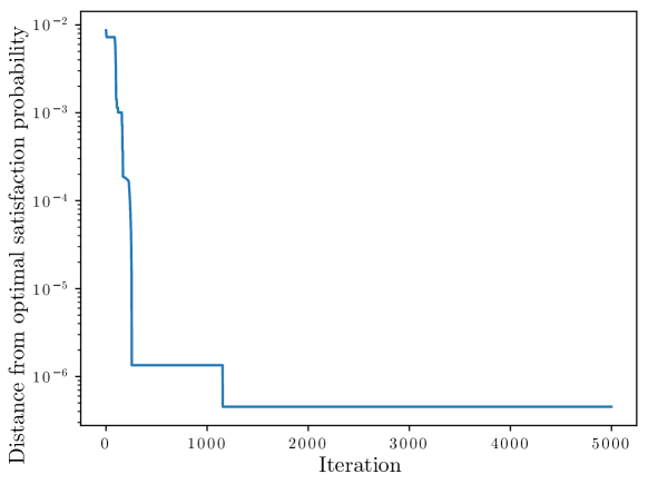
Figure 1: Distance from optimal satisfaction probability (found from MNE algorithm) across iterations for small test model

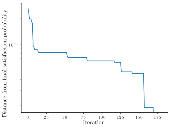
Figure 2: Distance from final satisfaction probability across iterations for UAV model with uniform wind

D.2 Runtimes

We have also considered how the various methods presented scale with both the number of sampled parameters, and the size of the MDP. In Figure 3, we see how the number of samples $N$ affects the runtime, evidently the work of Badings et al. (2022) scales approximately linearly (since they solve each sampled MDP). The deterministic solver based on the MaxMin game (explored further in Appendix E) and an MNE solver making use of fictitious self play to approximately solve for the equilibrium, clearly scale linearly, since they both must iterate through all samples to construct a reward matrix, but further computation is largely negligible. The solution based on iMDPs appears almost constant with respect to sample size, since we only need to find the maximum and minimum probabilities from amongst the samples this is roughly as expected (in fact we should expect linear scaling, but solving the iMDP takes longer and is independent of the sample size). Finally, for the subgradient and MNE solver using a PNS algorithm the results are more difficult to interpret, but may also be linear, as may be expected.

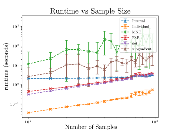
Figure 3: Runtime against number of samples

In Figure 4, we consider how the size of the MDP affects the runtimes of our various algorithms. The algorithms which require calculating a reward matrix scale approximately exponentially in the MDP size, and quickly start reaching computation limits. The other algorithms (ignoring some spurious initial behaviour), seem to scale roughly linearly with MDP size. For our subgradient algorithm this is as expected, since for each iteration we update every state-action pair individually. For the other algorithms, this is likely related to the model checker used to solve the models.

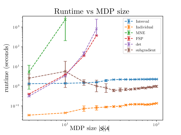
Figure 4: Runtime against size of MDP

Appendix E Deterministic MaxMin Policies

E.1 Finding MaxMin Deterministic Policies

One solution concept of interest involves finding the maximin deterministic policies for the game introduced in Section 3.2, through the use of a Stackelberg game (Stackelberg, 1952). To achieve this, the sample adversary acts as the leader and finds a minimising sample for each possible deterministic policy, that is, for every policy $\pi^{D}$, the adversary solves

$$r_{p}(\pi^{D})=\min_{u\in\mathcal{U}_{N}}\text{sol}_{\mathcal{M}}^{\pi^{D}}(u;\psi),$$ (16)

then the policy agent acts as the follower and chooses a deterministic policy which maximises the reward $r_{p}(\pi^{D})$. In this case, we are working with finite sets of actions for both agents, and so we can consider simply enumerating over all choices.

The resulting policy is the optimal deterministic policy, but may not be a Nash equilibrium policy (see Theorem 3.1). To see this note that if the sample adversary takes a fixed strategy (as opposed to always being allowed to choose the worst case), the policy agent may be able to improve their reward.

E.2 Probabilistic Guarantees under a MaxMin Deterministic Policy

In this case, our problem is degenerate, since it may be necessary to remove multiple constraints in order for another deterministic policy to become optimal, we therefore leverage techniques from Campi et al. (2018) for non-convex problems. This approach requires solving a different equation for the risk, $\mu(\tilde{s}^{\ast}_{N})$, which must satisfy (Campi et al., 2018, Theorem 1). One equation which satisfies these requirements is that in eq. 12.

The easiest method for obtaining an upper bound on the size of the support set is to consider the satisfaction probabilities for each deterministic policy in the worst-case MDP $\mathcal{M}[u^{\star}]$ for the optimal policy. If the satisfaction probability for a different policy is greater than the worst-case, then there must exist at least one sample that prevents us switching to that policy. As an upper bound, we may consider that every such policy is “blocked” by a single unique sample:

Alternatively, to improve this bound, we first find the set of “blocked” policies as above. Then, for each such policy, we find the samples which have an associated satisfaction probability less than our optimal $\lambda^{\star}$. To calculate the smallest support set, we then must find the smallest set such that at least one blocking sample for every policy is contained within this set. This problem is known as the hitting set problem and can be shown to be NP-hard. Alternatively, we may take a union of all sets to again find an upper bound.

Note that both methods may be computationally expensive if there are many possible deterministic policies.

We then have the following result that bounds the risk:

Corollary E.1.

We use eq. 12 to bound the risk. Bounds on the support constraints may be found as

$$\overline{\tilde{s}^{\ast}_{N}}=|\{\pi^{D}\in\Pi^{D}\colon Pr(\psi\>|\>\pi^{D},\mathcal{M}[u^{\star}])\geq\lambda^{\star}\}|,$$ (17)

or

$$\Sigma^{\ast}(\pi^{D}) =\{u\in\mathcal{U}_{N}\colon\text{sol}_{\mathcal{M}}^{\pi^{D}}(u;\psi)\leq\lambda^{\star}\wedge\text{sol}_{\mathcal{M}}^{\pi^{D}}(u^{\star};\psi)\geq\lambda^{\star}\}$$ (18)

$$\tilde{s}^{\ast}_{N} =\min_{\mathcal{V}\subseteq\mathcal{U}_{N}}|\mathcal{V}|\;\text{subject to:}\;\mathcal{V}\bigcap\Sigma^{\ast}(\pi^{D})\neq\emptyset,\forall\pi^{D}\in\Pi^{D},$$ (19)

the latter being less conservative, but significantly more computationally expensive. Approximate solutions to eq. 19 exist which may allow for a tradeoff between computation and optimality.

Then we have that

$$\mathbb{P}^{N}\left\{\mathbb{P}\left\{v\in\mathcal{V}\colon\mathcal{M}[v]\notsat_{\pi^{D}}\mathsf{P}_{\geq\lambda^{\star}}(\psi)\right\}\leq\mu(\tilde{s}^{\ast}_{N})\leq\mu(\overline{\tilde{s}^{\ast}_{N}})\right\}\geq 1-\beta,$$ (20)

where the only non-determinism arises due to the uncertainty in the transition function.

E.3 Results for Deterministic Policies

As is the case for our MNE algorithm, finding deterministic policies requires iterating through all possible deterministic policies. As such, we only have experimental results for our small toy model, we recall the results for our algorithms on this model, and provide results for the deterministic policy in Table 3.

	Sat. Prob. $\lambda^{\star}$	Risk U.B. $\overline{\epsilon}$	Time (s)	Emp. Risk $\tilde{\epsilon}$	Emp. (no pars)
Badings et al. (2022)	.338	.056	.07	.018	.115
iMDP Solver	.329	.155	1.39	.015	.107
MNE Algorithm	.333	.109	4.51	.043	.121
Subgradient Algorithm	.332	.285	26.12	.022	.115
Deterministic MaxMin Policy	.329	.105	0.28	.012	.105

Table 3: Results on Toy Model, with Deterministic Policies

References

- Arrow et al. (1953) K. J. Arrow, E. W. Barankin, D. Blackwell, R. Bott, N. Dalkey, M. Dresher, D. Gale, D. B. Gillies, I. Glicksberg, O. Gross, S. Karlin, H. W. Kuhn, J. P. Mayberry, J. W. Milnor, T. S. Motzkin, J. Von Neumann, H. Raiffa, L. S. Shapley, M. Shiffman, F. M. Stewart, G. L. Thompson, and R. M. Thrall. Contributions to the Theory of Games (AM-28), Volume II. Princeton University Press, 1953. ISBN 978-0-691-07935-6.
- Aussel et al. (1995) Didier Aussel, Jean-Noel Corvellec, and Marc Lassonde. Mean Value Property and Subdifferential Criteria for Lower Semicontinuous Functions. Transactions of the American Mathematical Society, 347(10):4147–4161, 1995. ISSN 0002-9947.
- Badings et al. (2022) Thom S. Badings, Murat Cubuktepe, Nils Jansen, Sebastian Junges, Joost-Pieter Katoen, and Ufuk Topcu. Scenario-based verification of uncertain parametric MDPs. Int. J. Softw. Tools Technol. Transf., 24(5):803–819, 2022.
- Badings et al. (2023) Thom S. Badings, Licio Romao, Alessandro Abate, David Parker, Hasan A. Poonawala, Mariëlle Stoelinga, and Nils Jansen. Robust Control for Dynamical Systems with Non-Gaussian Noise via Formal Abstractions. J. Artif. Intell. Res., 76:341–391, 2023.
- Baier and Katoen (2008) Christel Baier and Joost-Pieter Katoen. Principles of Model Checking. MIT Press, 2008. ISBN 978-0-262-02649-9.
- Belta et al. (2017) Calin Belta, Boyan Yordanov, and Ebru Aydin Gol. Formal Methods for Discrete-Time Dynamical Systems, volume 89 of Studies in Systems, Decision and Control. Springer International Publishing, Cham, 2017. ISBN 978-3-319-50762-0 978-3-319-50763-7. 10.1007/978-3-319-50763-7.
- Bhandari and Russo (2019) Jalaj Bhandari and Daniel Russo. Global optimality guarantees for policy gradient methods. CoRR, abs/1906.01786, 2019.
- Brunke et al. (2022) Lukas Brunke, Melissa Greeff, Adam W. Hall, Zhaocong Yuan, Siqi Zhou, Jacopo Panerati, and Angela P. Schoellig. Safe learning in robotics: From learning-based control to safe reinforcement learning. Annu. Rev. Control. Robotics Auton. Syst., 5:411–444, 2022.
- Calafiore and Campi (2006) Giuseppe Carlo Calafiore and Marco C. Campi. The scenario approach to robust control design. IEEE Trans. Autom. Control., 51(5):742–753, 2006.
- Campi and Garatti (2011) Marco C. Campi and Simone Garatti. A Sampling-and-Discarding Approach to Chance-Constrained Optimization: Feasibility and Optimality. J. Optim. Theory Appl., 148(2):257–280, 2011.
- Campi and Garatti (2018) Marco C. Campi and Simone Garatti. Wait-and-judge scenario optimization. Math. Program., 167(1):155–189, 2018.
- Campi et al. (2009) Marco C. Campi, Simone Garatti, and Maria Prandini. The scenario approach for systems and control design. Annu. Rev. Control., 33(2):149–157, 2009. 10.1016/j.arcontrol.2009.07.001.
- Campi et al. (2018) Marco Claudio Campi, Simone Garatti, and Federico Alessandro Ramponi. A General Scenario Theory for Nonconvex Optimization and Decision Making. IEEE Trans. Autom. Control., 63(12):4067–4078, 2018.
- Clarke et al. (2003) Edmund M. Clarke, Ansgar Fehnker, Zhi Han, Bruce H. Krogh, Olaf Stursberg, and Michael Theobald. Verification of Hybrid Systems Based on Counterexample-Guided Abstraction Refinement. In Hubert Garavel and John Hatcliff, editors, Tools and Algorithms for the Construction and Analysis of Systems, 9th International Conference, TACAS 2003, Held as Part of the Joint European Conferences on Theory and Practice of Software, ETAPS 2003, Warsaw, Poland, April 7-11, 2003, Proceedings, volume 2619 of Lecture Notes in Computer Science, pages 192–207. Springer, 2003. 10.1007/3-540-36577-X_14.
- Cubuktepe et al. (2022) Murat Cubuktepe, Nils Jansen, Sebastian Junges, Joost-Pieter Katoen, and Ufuk Topcu. Convex Optimization for Parameter Synthesis in MDPs. IEEE Trans. Autom. Control., 67(12):6333–6348, 2022.
- Daws (2004a) Conrado Daws. Symbolic and Parametric Model Checking of Discrete-Time Markov Chains. In ICTAC, volume 3407 of Lecture Notes in Computer Science, pages 280–294. Springer, 2004a.
- Daws (2004b) Conrado Daws. Symbolic and Parametric Model Checking of Discrete-Time Markov Chains. In ICTAC, volume 3407 of Lecture Notes in Computer Science, pages 280–294. Springer, 2004b.
- Foster (1962) F. G. Foster. Dynamic Programming and Markov Processes. By R. A. Howard. Pp. 136. 46s. 1960. (John Wiley and Sons, N.Y.). The Mathematical Gazette, 46(358):340–341, December 1962. ISSN 0025-5572, 2056-6328.
- Frihauf et al. (2012) Paul Frihauf, Miroslav Krstic, and Tamer Basar. Nash equilibrium seeking in noncooperative games. IEEE Trans. Autom. Control., 57(5):1192–1207, 2012.
- Garatti and Campi (2022) Simone Garatti and Marco C. Campi. Risk and complexity in scenario optimization. Math. Program., 191(1):243–279, 2022. 10.1007/s10107-019-01446-4.
- Hahn et al. (2011a) Ernst Moritz Hahn, Tingting Han, and Lijun Zhang. Synthesis for PCTL in Parametric Markov Decision Processes. In Mihaela Gheorghiu Bobaru, Klaus Havelund, Gerard J. Holzmann, and Rajeev Joshi, editors, NASA Formal Methods - Third International Symposium, NFM 2011, Pasadena, CA, USA, April 18-20, 2011. Proceedings, volume 6617 of Lecture Notes in Computer Science, pages 146–161. Springer, 2011a. 10.1007/978-3-642-20398-5_12.
- Hahn et al. (2011b) Ernst Moritz Hahn, Holger Hermanns, and Lijun Zhang. Probabilistic reachability for parametric Markov models. Int. J. Softw. Tools Technol. Transf., 13(1):3–19, 2011b.
- Hansson and Jonsson (1994) Hans Hansson and Bengt Jonsson. A logic for reasoning about time and reliability. Formal Aspects of Computing, 6(5):512–535, September 1994. ISSN 1433-299X. 10.1007/BF01211866.
- Heinrich et al. (2015) Johannes Heinrich, Marc Lanctot, and David Silver. Fictitious Self-Play in Extensive-Form Games. In ICML, volume 37 of JMLR Workshop and Conference Proceedings, pages 805–813. JMLR.org, 2015.
- Hensel et al. (2022) Christian Hensel, Sebastian Junges, Joost-Pieter Katoen, Tim Quatmann, and Matthias Volk. The probabilistic model checker Storm. Int. J. Softw. Tools Technol. Transf., 24(4):589–610, 2022.
- Iyengar (2005) Garud N. Iyengar. Robust Dynamic Programming. Math. Oper. Res., 30(2):257–280, 2005.
- Junges et al. (2019) Sebastian Junges, Erika Ábrahám, Christian Hensel, Nils Jansen, Joost-Pieter Katoen, Tim Quatmann, and Matthias Volk. Parameter Synthesis for Markov Models. CoRR, abs/1903.07993, 2019.
- Kiwiel (2001) Krzysztof C. Kiwiel. Convergence and efficiency of subgradient methods for quasiconvex minimization. Math. Program., 90(1):1–25, 2001.
- Knight (2002) John C. Knight. Safety critical systems: Challenges and directions. In Will Tracz, Michal Young, and Jeff Magee, editors, Proceedings of the 24th International Conference on Software Engineering, ICSE 2002, 19-25 May 2002, Orlando, Florida, USA, pages 547–550. ACM, 2002. 10.1145/581339.581406.
- Kozine and Utkin (2002) Igor Kozine and Lev V. Utkin. Interval-Valued Finite Markov Chains. Reliab. Comput., 8(2):97–113, 2002.
- Kwiatkowska et al. (2011) Marta Z. Kwiatkowska, Gethin Norman, and David Parker. PRISM 4.0: Verification of probabilistic real-time systems. In CAV, volume 6806 of Lecture Notes in Computer Science, pages 585–591. Springer, 2011.
- Meedeniya et al. (2014) Indika Meedeniya, Irene Moser, Aldeida Aleti, and Lars Grunske. Evaluating probabilistic models with uncertain model parameters. Softw. Syst. Model., 13(4):1395–1415, 2014.
- Nash (1989) John Nash. Non-cooperative games. Cournot Oligopoly, pages 82–94, January 1989. 10.1017/CBO9780511528231.007.
- Nilim and Ghaoui (2005) Arnab Nilim and Laurent El Ghaoui. Robust Control of Markov Decision Processes with Uncertain Transition Matrices. Oper. Res., 53(5):780–798, 2005.
- Osband et al. (2019) Ian Osband, Benjamin Van Roy, Daniel J. Russo, and Zheng Wen. Deep exploration via randomized value functions. J. Mach. Learn. Res., 20:124:1–124:62, 2019.
- Platzer (2012) André Platzer. Logics of Dynamical Systems. In Proceedings of the 27th Annual IEEE Symposium on Logic in Computer Science, LICS 2012, Dubrovnik, Croatia, June 25-28, 2012, pages 13–24. IEEE Computer Society, 2012. 10.1109/LICS.2012.13.
- Porter et al. (2008) Ryan Porter, Eugene Nudelman, and Yoav Shoham. Simple search methods for finding a Nash equilibrium. Games Econ. Behav., 63(2):642–662, 2008.
- Puggelli et al. (2013) Alberto Puggelli, Wenchao Li, Alberto L. Sangiovanni-Vincentelli, and Sanjit A. Seshia. Polynomial-Time Verification of PCTL Properties of MDPs with Convex Uncertainties. In CAV, volume 8044 of Lecture Notes in Computer Science, pages 527–542. Springer, 2013.
- Quatmann et al. (2016) Tim Quatmann, Christian Dehnert, Nils Jansen, Sebastian Junges, and Joost-Pieter Katoen. Parameter synthesis for markov models: Faster than ever. In ATVA, volume 9938 of Lecture Notes in Computer Science, pages 50–67, 2016.
- Raskin and Sankur (2014) Jean-François Raskin and Ocan Sankur. Multiple-Environment Markov Decision Processes. In FSTTCS, volume 29 of LIPIcs, pages 531–543. Schloss Dagstuhl - Leibniz-Zentrum für Informatik, 2014.
- Rickard et al. (2023) Luke Rickard, Thom Badings, Licio Romao, and Alessandro Abate. Formal Controller Synthesis for Markov Jump Linear Systems with Uncertain Dynamics, May 2023.
- Scheftelowitsch et al. (2017) Dimitri Scheftelowitsch, Peter Buchholz, Vahid Hashemi, and Holger Hermanns. Multi-Objective Approaches to Markov Decision Processes with Uncertain Transition Parameters. In VALUETOOLS, pages 44–51. ACM, 2017.
- Stackelberg (1952) H. Von. Stackelberg. The Theory of Market Economy. Translated from the German and with an Introduction by A.T. Peacock. London, Edinburgh, Glasgow, W. Hodge & Co, Ltd., 1952, xxiii p. 328 p., 25/-. Recherches Économiques de Louvain/ Louvain Economic Review, 18(5):543–543, 1952. ISSN 1373-9719. 10.1017/S0770451800047382.
- van der Vegt et al. (2023) Marck van der Vegt, Nils Jansen, and Sebastian Junges. Robust Almost-Sure Reachability in Multi-Environment MDPs. In TACAS (1), volume 13993 of Lecture Notes in Computer Science, pages 508–526. Springer, 2023.
- Wiesemann et al. (2013) Wolfram Wiesemann, Daniel Kuhn, and Berç Rustem. Robust Markov Decision Processes. Math. Oper. Res., 38(1):153–183, 2013.
- Yousefimanesh et al. (2023) Niloofar Yousefimanesh, Iwan Bos, and Dries Vermeulen. Strategic rationing in Stackelberg games. Games Econ. Behav., 140:529–555, 2023.
- Yu and Dimarogonas (2021) Pian Yu and Dimos V. Dimarogonas. Distributed motion coordination for multi-robot systems under LTL specifications, March 2021.