RankMatch: A Novel Approach to Semi-Supervised Label Distribution Learning Leveraging Inter-label Correlations

Abstract

This paper introduces RankMatch, an innovative approach for Semi-Supervised Label Distribution Learning (SSLDL). Addressing the challenge of limited labeled data, RankMatch effectively utilizes a small number of labeled examples in conjunction with a larger quantity of unlabeled data, reducing the need for extensive manual labeling in Deep Neural Network (DNN) applications. Specifically, RankMatch introduces an ensemble learning-inspired averaging strategy that creates a pseudo-label distribution from multiple weakly augmented images. This not only stabilizes predictions but also enhances the model’s robustness. Beyond this, RankMatch integrates a pairwise relevance ranking (PRR) loss, capturing the complex inter-label correlations and ensuring that the predicted label distributions align with the ground truth. We establish a theoretical generalization bound for RankMatch, and through extensive experiments, demonstrate its superiority in performance against existing SSLDL methods.

1 Introduction

Label Distribution Learning (LDL) (Geng, 2016) is an innovative machine learning paradigm to tackle the issue of label ambiguity. Unlike multi-label learning (MLL) (Zhang & Zhou, 2014), LDL assigns not only a specific number of labels to each instance but also the importance degree of each label. For instance, as shown in Fig. 1, an example from a facial emotion dataset(Shih et al., 2008) is displayed, as well as the annotated label distribution. The importance degree is referred to as the label description degree (Geng, 2016; Jia et al., 2023), which offers more comprehensive semantic information. Recent studies have witnessed the significant advancements made by LDL in various practical applications, such as expression recognition (Chen et al., 2020), facial age estimation (Geng et al., 2013), image object detection (Xu et al., 2023), joint acne image grading (Wu et al., 2019) and head-pose estimation (Liu et al., 2019).

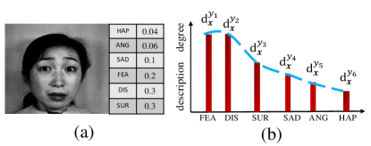
Figure 1: An illustration of an example from a facial SJAFFE dataset (Shih et al., 2008) annotated with a label distribution.

The success of deep learning heavily rely on large-scale and accurately labeled datasets, which are necessary to train very deep neural networks (DNNs) with superior generalization. However, acquiring such labeled data can be an arduous and costly process. Especially, it is more costly to obtain large dataset annotated with label distribution. For instance, considering the RAF-LDL dataset (Li & Deng, 2019), 315 trained annotators were employed, and each image is annotated for enough independent times to get the appropriate label distribution. As a result, the conflict emerges prominently when LDL embraces DNNs. A possible way to address the challenge is to leverage the highly available unlabeled data. In this paper, we present the semi-supervised LDL (SSLDL), which aims to develop an LDL model with a few labeled data and a larger pool of unlabeled data.

Notice that semi-supervised learning (SSL) has already make significant advancements (Basak & Yin, 2023; Fini et al., 2023), especially in the era of deep learning. However, SSLDL has not been explored to the same extent. Traditional SSL approaches are mainly designed for SLL or MLL, which often rely on confidence-based pseudo-labeling (Jiang et al., 2022), (Sohn et al., 2020) and fall in SSLDL because its goal is to predict the whole label distribution, not just the most likely label. Moreover, exiting SSL methods typically ignore the correlation between labels (Xu & Zhou, 2017), potentially hindering their performance for LDL.

To solve the challenging SSLDL problem, we put forward in the paper a novel SSLDL method called RankMatch. It uses an averaging strategy from the ensemble learning (Zhou & Zhou, 2021), taking the mean of predictions from variously augmented images (Sohn et al., 2020) to form a pseudo label distribution. RankMatch approach aims to stabilize the predictions and improve model robustness. Moreover, RankMatch incorporates a pairwise relevance ranking loss to acknowledge and utilize the relationships between labels, aligning the predicted label distributions with the ground truth. In the theoretical analysis, we establish a generalization bound for RankMatch. Finally, in the experiments, we demonstrate that RankMatch can effectively address the SSLDL problem and outperform existing methods.

In summary, our contributions can be summarized as

• To the best of our knowledge, this is the first work employing deep learning to address the SSLDL problem.

• We propose the RankMatch approach that leverages inter-label correlations to tackle the SSLDL problem.

• We establish a theoretical generalization bound for RankMatch and validate its efficacy through extensive experimentation.

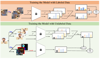
Figure 2: Overview of the RankMatch Algorithm for Semi-Supervised Label Distribution Learning: The diagram showcases the model training phases, where the locked icon indicates phases with fixed parameters and the unlocked icon represents parameter updates. The top (orange) delineates the process with labeled data, while the bottom (green) details the approach for integrating unlabeled data.

2 RELATED WORK

2.1 Label Distribution Learning

Label distribution learning (LDL) (Geng, 2016) is an innovative learning approach that assigns a label distribution to each instance and directly learns a mapping from instances to these label distributions. The initial proposal of LDL was aimed at addressing the problem of facial age estimation (Geng et al., 2013). It involves the label distributions generated for all age groups, which is considered more advantageous than relying on a single age label. Next, Geng(Geng, 2016) discovered that in some practical applications, it is more preferable to have distributions spanning all labels rather than associating a single label with an instance(Xu & Zhou, 2017). Such as, in the task of facial emotion recognition, the human emotions are often a blend of multiple emotional states rather than a single one. Because LDL can model the uncertainty of the label space, it has been receiving increasing attention. To name some examples, NASA employs LDL for predicting mineral compositions in Martian meteorite craters (Morrison et al., 2018). In this research, they fine-tuned the LDL algorithm to predict the chemical elements (labels) and their abundances (degrees) for each Martian mineral sample based on crystallographic parameters. The research by (Zhou et al., 2020) addresses the challenge of facial expression variations in depression recognition by framing it as a label distribution learning (LDL) task. Their innovative Deep Joint Label Distribution and Metric Learning (DJ-LDML) approach effectively navigates the nuanced differences in facial expressions, both within the same depression level and across different levels, enhancing the accuracy of depression assessment. In indoor videos, people often remain relatively still for extended periods. Based on this observation, Ling (Ling & Geng, 2019) employs label distributions to cover a certain number of crowd count labels, representing the level of description each label provides for video frames, in order to address the crowd counting problem in indoor videos.

2.2 Semi-supervised Label Distribution Learning

Lack of sufficient training data with exact labels is still a challenge for label distribution learning. To deal with such problem, many algorithms have been proposed, known as Semi-Supervised Label Distribution Learning (SSLDL). To named some, Hou (Hou et al., 2017) uses the average of labels from the neighbors of unlabeled data as its label distribution, and then trains the LDL model with both labeled and unlabeled data. Jia (Jia et al., 2021b) recovers unknown label distributions by utilizing sample-related information among graph nodes. Liu (Liu et al., 2022) proposed a semi-supervised label distribution learning algorithm based on co-regularization, which employs two different model structures to handle labeled and unlabeled data, demonstrating strong robustness and consistency.

Although a range of SSLDL approaches have been proposed, they are not end-to-end. Traditional methods typically necessitate manual feature engineering and struggle with large-scale, high-dimensional data, while also inadequately leveraging unlabeled data. In contrast, deep learning is renowned for its ability to autonomously learn complex feature representations and has proven effective in various data-intensive tasks. Thus, we are motivated to explore the potential of deep learning in addressing SSL challenges, with the aim of overcoming the limitations inherent in conventional techniques.

3 The Method

3.1 Problem Statement and Notation

In semi-supervised label distribution learning (SSLDL), we have a training set denoted by $\mathcal{D}$, which combines labeled and unlabeled datasets: $\mathcal{D}_{L}=\{(\mathbf{x}_{i},\mathbf{d}_{i})|i\leq n\}$ for labeled samples and $\mathcal{D}_{U}=\{\mathbf{x}_{j}|j\leq m\}$ for unlabeled samples. The instance variable is denoted by $\mathbf{x}$, the particular i-th instance is denoted by $\mathbf{x}_{i}$, $\mathbf{d_{i}}=\{d^{y_{1}}_{\mathbf{x_{i}}},d^{y_{2}}_{\mathbf{x_{i}}},...,d^{y_{c}}_{\mathbf{x_{i}}}\}$ represents the label distribution for instance $\mathbf{x}_{i}$, where c is the number of label, and $d_{\mathbf{x}_{i}}^{y_{c}}$ reflects the relevance of label $y_{c}$ to the instance, and $\sum_{j=1}^{c}d_{\mathbf{x}_{i}}^{y_{j}}=1$. Our goal is to train a deep neural network (DNN), represented as $f(\mathbf{x};\theta)$, to predict these label distributions. The model’s output for each label $y_{j}$ is normalized using the Softmax function (Jang et al., 2016) to ensure a proper probability distribution:

$$h(y_{j}|{\mathbf{x}}_{i};\theta)=\frac{\exp(f_{j}(\mathbf{x}_{i};\theta))}{\sum_{q}\exp(f_{q}(\mathbf{x}_{i};\theta))},$$ (1)

where $f_{j}(\mathbf{x}_{i};\theta)$ is the raw output of the DNN for label $y_{j}$ and the instance $\mathbf{x}_{i}$, and the denominator is the sum over all possible labels, ensuring the output for each instance sums to 1 (Gao et al., 2017). This way, $h(y_{j}|x_{i};\theta)$ provides a normalized prediction of label $y_{j}$’s relevance for each instance $\mathbf{x}_{i}$.

3.2 The Supervised Loss

In label distribution learning, we diverge from the traditional binary cross-entropy loss used in multi-label learning (Hershey & Olsen, 2007) , as LDL requires predicting a range of label intensities rather than separate binary outcomes. We use Kullback-Leibler (KL) divergence (Hershey & Olsen, 2007) as the loss function to measure the difference between the predicted and actual label distributions. The supervised loss is defined as

$$\mathcal{L}_{s}=\frac{1}{n}\sum_{i=1}^{n}\sum_{j=1}^{q}d_{\mathbf{x}_{i}}^{y_{j}}\ln\left(\frac{d_{\mathbf{x}_{i}}^{y_{j}}}{h(y_{j}\mid\operatorname{Aug}_{w}(\mathbf{x}_{i}))}\right),$$ (2)

where $\operatorname{Aug}_{w}(\mathbf{x}_{i})$ indicates the weak augmentation applied to the $i$-th sample, and $h(y_{j}\mid\operatorname{Aug}_{w}(\mathbf{x}_{i}))$ is the DNN’s predicted probability for label $y_{j}$. This loss encourages the model to align closely with the true label distribution.

3.3 The Unsupervised Consistency Loss

In semi-supervised label distribution learning, the challenge lies in leveraging both the labeled and the significant volume of unlabeled data effectively. Consistency regularization emerges as a potent strategy, drawing inspiration from recent advancements in SSL (Jiang et al., 2022) (Sohn et al., 2020) (Yang et al., 2022) (Zhang et al., 2021). The principle driving this approach is ensuring that the classifier’s output remains stable across different augmentations of the same unlabeled instance, thereby reinforcing the reliability of the label distribution predictions.

To enhance the stability of predictions and tap into the full potential of unlabeled data, we employ an ensemble learning-inspired technique (Zhou & Zhou, 2021). Rather than relying on high-confidence predictions, we average the outputs from multiple weakly augmented (Sohn et al., 2020) variants of the same unlabeled image. This process forms what we call the pseudo-label distribution (PLD) for each unlabeled instance, described as $\mathbf{p}_{i}$, which aggregates the predictions across augmentations and smooths out anomalies due to random variance in the data augmentation process. The unsupervised consistency loss, $\mathcal{L}_{uc}$, is then calculated by contrasting the PLD with the model’s predictions for strongly augmented (Sohn et al., 2020) versions of the same instances. The formula is given by

$$\mathcal{L}_{uc}=\frac{1}{m}\sum_{u=1}^{m}\sum_{j=1}^{q}\left(p_{\mathbf{x}_{u}}^{y_{j}}\ln\left(\frac{p_{\mathbf{x}_{u}}^{y_{j}}}{h\left(y_{j}\mid\operatorname{Aug}_{s}(\mathbf{x}_{u})\right)}\right)\right),$$ (3)

where $h\left(y_{j}\mid\operatorname{Aug}_{s}(\mathbf{x}_{u})\right)$ represents the prediction for label $y_{j}$ post strong augmentation (Sohn et al., 2020). This loss function plays a pivotal role in SSLDL by guiding the model to learn from the structure within the data, even when explicit labels are not available.

3.4 The Pairwise Relevance Ranking Loss

The supervised loss and the unsupervised consistency loss both treat the predicted results and ground-truth (or PLD) as multiple independent prediction tasks, thereby overlooking the inter-label correlation (Xu & Zhou, 2017), which may lead to a decrease in performance. In LDL, a sample is assigned multiple label description degree , and these description degree are often not completely independent of each other (Jia et al., 2018). The correlation between the description degrees can be either positive or negative. For example, if an image $\mathbf{x}$ has a label distribution of $d_{\mathbf{x}}^{y_{1}}=0.4$ and $d_{\mathbf{x}}^{y_{2}}=0.2$, we consider labels $y_{1}$ and $y_{2}$ to be negatively correlated. Similarly, if the labels have a distribution of $d_{\mathbf{x}}^{y_{1}}=0.4$ and $d_{\mathbf{x}}^{y_{2}}=0.4$, we consider labels $y_{1}$ and $y_{2}$ to be positively correlated. This pairwise ranking relationship implicitly expresses the label correlation between label distributions.

To tackle this challenge, we introduce a pairwise relevance ranking (PRR) loss $\mathcal{L}_{PRR}$ to align this inherent semantic structure. For labeled data, we aim for a strict alignment between the ranking of predicted label distributions and the ground-truth. This means that we not only need to align the ranking relationships between label descriptions but also maintain the margin with the ground-truth. Additionally, for certain ”close” description degrees, studying their ranking is not meaningful. For instance, consider a scenario where the label description degrees $d_{\mathbf{x}}^{y_{i}}$ and $d_{\mathbf{x}}^{y_{k}}$ are 0.32 and 0.33, respectively. The negligible discrepancy between these two values could be attributed to variations in annotation. Consequently, we opt not to adjust their ranking order to account for such minor differences, which may not reflect actual dissimilarities in label importance. Simplifying our notation, let $h_{j}(\mathbf{x}_{i})$ represent the predicted degree of relevance for the j-th label after applying a weak augmentation $\operatorname{Aug}_{w}$ to the i-th instance. The $\mathcal{L}_{PRR_{L}}$ loss is then defined as follows:

$$\mathcal{L}_{PRR_{L}}= \sum_{1<j<k<q}I(d_{\mathbf{x}_{i}}^{y_{j}},d_{\mathbf{x}_{i}}^{y_{k}})\cdot\max(0,\delta-(h_{j}(\mathbf{x}_{i})-h_{k}(\mathbf{x}_{i})))$$ (4)

$$+I(d_{\mathbf{x}_{i}}^{y_{k}},d_{\mathbf{x}_{i}}^{y_{j}})\cdot\max(0,\delta-(h_{k}(\mathbf{x}_{i})-h_{j}(\mathbf{x}_{i}))),$$

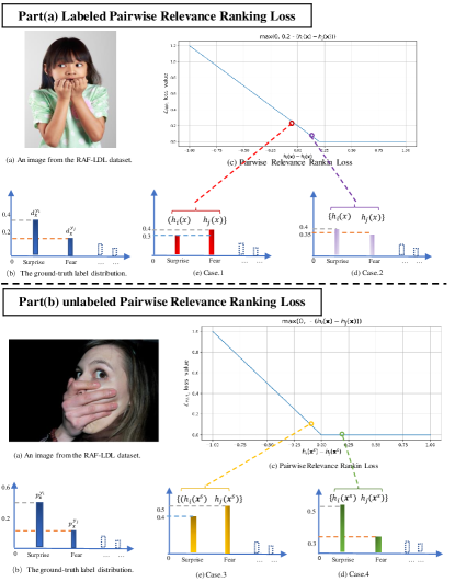
Figure 3: An examples to illustrate the $\mathcal{L}_{PRR}$ loss.

Fig. 3, Part (a), presents an image from the RAF-LDL dataset and its label distribution, illustrating the application of the $\mathcal{L}_{PRR_{L}}$ loss. Here, $\delta=d_{\mathbf{x}_{i}}^{y_{k}}-d_{\mathbf{x}_{i}}^{y_{j}}$ and the function $I(d_{\mathbf{x}_{i}}^{y_{j}},d_{\mathbf{x}_{i}}^{y_{k}})$ is an indicator that outputs 1 if the first label’s degree is greater than the second’s and their difference is significant, i.e., $d_{\mathbf{x}_{i}}^{y_{j}}>d_{\mathbf{x}_{i}}^{y_{k}}$ and $|d_{\mathbf{x}_{i}}^{y_{j}}-d_{\mathbf{x}_{i}}^{y_{k}}|>t$. The loss comes into play in two key scenarios: Case 1, when the model’s predicted ranking of labels is incorrect, and Case 2, when the ranking is correct but the margin does not align with the ground truth. Both cases indicate opportunities for the model to learn and adjust its predictions.

In the unsupervised component of our model, we confront the absence of ground-truth labels by employing pseudo-label distributions (PLDs) as a stand-in during training. Recognizing that PLDs may not always be precise, we focus on aligning the predicted pairwise relevance rankings of label descriptions to mitigate the potential for overfitting and to correct inaccuracies inherent in SSL. We define the unsupervised pairwise relevance ranking loss, $\mathcal{L}_{PRR_{u}}$, where $h_{j}(\mathbf{x}_{i}^{s})$ denotes the predicted relevance of the j-th label after strong augmentation, $\operatorname{Aug}_{s}$, is applied to the i-th instance. The loss function is as follows:

$$\mathcal{L}_{PRR_{u}}= \sum_{1<j<k<q}I(p_{\mathbf{x}_{i}}^{y_{j}},p_{\mathbf{x}_{i}}^{y_{k}})\cdot\max(0,-(h_{j}(\mathbf{x}_{i}^{s})-h_{k}(\mathbf{x}_{i}^{s})))$$ (5)

$$+I(p_{\mathbf{x}_{i}}^{y_{k}},p_{\mathbf{x}_{i}}^{y_{j}})\cdot\max(0,-(h_{k}(\mathbf{x}_{i}^{s})-h_{j}(\mathbf{x}_{i}^{s}))),$$

where the indicator function, $I(p_{\mathbf{x}_{i}}^{y_{j}},p_{\mathbf{x}_{i}}^{y_{k}})$, outputs 1 if the pseudo-label of one label is greater than the other and their difference is substantial, specifically when $p_{\mathbf{x}_{i}}^{y_{j}}>p_{\mathbf{x}_{i}}^{y_{k}}$ and the difference $|p_{\mathbf{x}_{i}}^{y_{j}}-p_{\mathbf{x}_{i}}^{y_{k}}|$ exceeds a threshold $t$; otherwise, it outputs 0. This loss addresses the scenario where the model’s ranking of label predictions is inaccurate, as illustrated in Fig. 3, Part (b). Here, we see an image from the RAF-LDL dataset and its associated pseudo-label distribution. For example, when the PLD for surprise ($p_{\mathbf{x}}^{y_{i}}$) is 0.6 and for fear ($p_{\mathbf{x}}^{y_{j}}$) is 0.2, the $\mathcal{L}_{PRR}$ loss is activated as $\max(0,-(h_{i}(\mathbf{x})-h_{j}(\mathbf{x})))$, emphasizing the need for the model to correct the predicted rankings to reflect the pseudo-labels more accurately.

In conclusion, the RankMatch algorithm, as illustrated in Fig. 2, harnesses a dual-phase training strategy for semi-supervised label distribution learning. It differentiates between the treatment of labeled and unlabeled data, refining the model with fixed parameters for the former and updating parameters for the latter. Our tailored loss function combines supervised and unsupervised ranking losses under the PRR framework, with a lambda ($\lambda$) coefficient to balance their influence. Thus, the total loss is defined as $\text{loss}=\mathcal{L}_{s}+\mathcal{L}_{uc}+\lambda(\mathcal{L}_{PRR_{L}}+\mathcal{L}_{PRR_{u}})$, streamlining the model’s learning from both labeled and unlabeled datasets.

3.5 Theoretical Analysis

In this section, we establish a theoretical foundation for our RankMatch algorithm within the realm of Semi-Supervised Label Distribution Learning (SSLDL) by defining a generalization bound.

3.5.1 Generalization Bound

Theorem 1.

For any function $f$ in $\mathcal{F}_{\beta,\nu}$ (Jiang et al., 2023), the following inequality is satisfied with probability at least $1-\delta$ over the random selection of $\mathcal{D}_{L}$ and $\mathcal{D}_{U}$:

$$R_{\text{-KL }}(f) \leq C_{1}\cdot\widehat{R}_{\mathcal{D}_{U}}(f)+C_{2}\left(1+\frac{C_{0}}{2}\right)\cdot\widehat{R}_{\mathcal{D}_{L}}(f)$$

$$+C_{1}(\frac{16Kq}{\sqrt{m}}\cdot\frac{1-\varepsilon}{\varepsilon}\left[1+3\sqrt{W_{g}\cdot\log\left(C_{M}m\right)}\right]$$

$$+3\sqrt{\frac{\log\frac{4}{\delta}}{2m}})+\frac{3C_{0}C_{2}}{2}\cdot\Psi_{n,q,\delta}\left(\mathcal{F}_{\beta,m}\right),$$

where $\hat{R}_{D_{L}}(f)$ and the latter by $\hat{R}_{D_{U}}(f)$ denote the empirical risk on labeled and unlabeled datasets, $C_{0}$ is a universal constant, $C_{1}$ and $C_{2}$ are constants determined by the neural network capacity and the structure of the data distribution, $\varepsilon\in(0,0.5)$. And the last term is the complexity terms and they are dominated by the upper bound of the Rademacher complexity. Specifically, $\Psi_{n,q,\delta}(\mathcal{F}_{\beta,m})$ are given by

$$\Psi_{n,q,\delta}(\mathcal{F}_{\beta,\nu})= 2(\sqrt{q}\cdot\log^{3/2}(nqe)\cdot\psi_{n,q}(\mathcal{F}_{\beta,\nu})$$

$$+\frac{1}{\sqrt{n}})+\frac{\log(qe)}{n}\left(\log\frac{2}{\delta}+\log(\log n)\right).$$

$$\psi_{n,q}(\mathcal{F}_{\beta,m})=\frac{4}{\sqrt{n\cdot q}}+\frac{12}{\sqrt{n\cdot q}}\sqrt{W\cdot\log(C_{N}\sqrt{nq})},$$

The left-hand side of the inequality, $R_{KL}(f)$, represents the expected robust risk when measured with the KL divergence. The right-hand side aggregates the empirical risks and a series of complexity terms, encapsulating the Rademacher complexity. The detailed proof of Theorem 1, which includes the definitions and derivations of the Rademacher complexity terms as well as the constants $C_{0}$, $C_{1}$, $C_{2}$,$C_{M}$, $C_{N}$ and the set $\mathcal{B}_{sem}(x_{i}^{u})$, is located in the appendix. This proof lays the groundwork for asserting the model’s efficacy and robustness in learning from both labeled and unlabeled data in an SSLDL setting.

Remark 1.

Theorem 1 implies that the third term is of order $O\left(K\sqrt{\frac{W_{g}\log m}{m}}\right)$, and the fourth term is of order $\Psi_{n,q,\delta}\left(\mathcal{F}_{\beta,\nu}\right)$, more specifically, in $O\left(\log^{2}\left(nq\right)\sqrt{\frac{W}{n}}\right)$. Therefore, the order of the generalization gap is $O\left(K\sqrt{\frac{W_{g}\cdot\log m}{m}}+\log^{2}\left(nq\right)\sqrt{\frac{W}{n}}\right)$.

3.6 Experiments

3.6.1 Experimental Configurations

Experimental Datasets :In this paper, we validate our approach using four distinct real-world datasets. The details of these datasets are as follows:

Twitter-LDL (Yang et al., 2017): A large-scale Visual Sentiment Distribution dataset was constructed from Twitter, encompassing eight distinct emotions Amusement, Anger, Awe, Contentment, Disgust, Excitement, Fear, Sadness. Approximately 30,000 images were collected by searching various emotional keywords, such as ”sadness,” ”heartbreak,” and ”grief.” Subsequently, eight annotators were hired to label this dataset. The resulting Twitter LDL dataset comprises 10,045 images.

Flickr-LDL (Yang et al., 2017): A subset of the Flickr dataset (Borth et al., 2013), unlike other datasets that searched for images using emotional terms, the Flickr dataset collected 1,200 pairs of adjective-noun pairs, resulting in 500,000 images. We employed 11 annotators to label this subset with tags for eight common emotions. In the end, the Flickr LDL was created, containing 10,700 images, with roughly equal quantities for each class.

Emotion6 (Peng et al., 2015): Emotion6: We collected 1,980 images from Flickr (Borth et al., 2013) using six category keywords and synonyms as search terms for Emotion6. A total of 330 images were collected for each category, and each image was assigned to only one category (dominant emotion). Emotion6 represents the emotions related to each image in the form of a probability distribution, consisting of 7 bins, including Ekman’s 6 basic emotions (Carroll & Russell, 1996) and neutral.

RAF-LDL (Li & Deng, 2019): RAF-LDL is a multi-label distribution facial expression dataset, comprising approximately 5,000 diverse facial images downloaded from the internet. These images exhibit variations in emotion, subject identity, head pose, lighting conditions, and occlusions. During annotation, 315 well-trained annotators are employed to ensure each image can be annotated enough independent times. And images with multi-peak label distribution are selected out to constitute the RAF-LDL.

Comparing methods In order to assess the effectiveness of the proposed approach, we benchmark it against four sets of methods: 1) The first group consists of two deep learning SSLDL algorithms that we introduced, named FixMatch-LDL (Sohn et al., 2020) and MixMatch-LDL (Peng et al., 2015). Since there are currently no open-source semi-supervised LDL works in deep learning, these two algorithms were developed by us, based on the current most effective two deep learning SSL algorithms. 2) The second group of algorithms is a deep learning SSLDL algorithm based on the dual-network concept (Chen et al., 2021), which we named GCT-LDL. The core idea involves mutual supervision of the outputs from two independent networks using unlabeled data. 3) The third group consists of traditional SSLDL algorithms, referred to as SA-LDL (Hou et al., 2017). Since SA-LDL is an SSLDL algorithm designed for tabular data, we needed to perform feature engineering on image data, the details can be found in appendix. 4) The fourth category consists of existing LDL algorithms. As there is currently only one open-source SSLDL algorithm, which is SA-LDL (Hou et al., 2017), we compared it with some state-of-the-art LDL algorithms. In this regard, we selected four state-of-the-art LDL algorithms: Adam-LDL-SCL (Jia et al., 2019), sLDLF (Shen et al., 2017), DF-LDL (González et al., 2021), and LDL-LRR (Jia et al., 2021a). These methods are designed for fully labeled LDL algorithms and may not be suitable for the SSLDL problem. All algorithm details and configurations can be found in the appendix.

Implementation Following (Cole et al., 2021), we employ ResNet-50 (He et al., 2016) pre-trained on ImageNet (Krizhevsky et al., 2012) for training the classification model. For training images, we adopt standard flip-and-shift strategy (Sohn et al., 2020) for weak data augmentation, and RandAugment (Cubuk et al., 2020) and Cutout (DeVries & Taylor, 2017) for strong data augmentation. We employ AdamW (You et al., 2019) optimizer and one-cycle policy scheduler (Hannan et al., 2021) to train the model with maximal learning rate of 0.0001. For all datasets, the number of epochs is set as 30 and the batch size is set as 32. Furthermore, we perform exponential moving average (EMA) (Klinker, 2011) for the model parameter $\theta$ with a decay of 0.98. We adjust the parameter $\lambda$ across a range of values, specifically $\{0.005,0.01,0.05,0.1\}$. We perform all experiments on GeForce RTX 3090 GPUs. The random seed is set to 1 for all experiments.

Evaluation Metrics: In evaluating LDL methods, we employ six distinct metrics (Geng, 2016): Chebyshev, Clark, and Canberra distances, along with Kullback-Leibler divergence, where lower values are preferable, and Intersection and Cosine similarities, where higher values indicate better performance. Details of the evaluation metrics are provided in the Appendix.

3.6.2 Comparative Experiment Analysis

We employed a range of labeled data proportions (10%, 20%, and 40%) to simulate varying levels of label availability, a critical factor in semi-supervised learning scenarios. Our evaluation metrics included Canberra and Clark distances, Intersection and Cosine similarities, and KL divergence—providing a multifaceted evaluation of predictive performance.

The results, as displayed in Table. 1 and Table. 2, reveal a consistent pattern of superior performance by the RankMatch algorithm. Particularly, it exhibits lower scores in Canberra and Clark distances across all datasets and sample proportions, signifying its ability to minimize prediction errors effectively. This is indicative of RankMatch’s capacity to capture the intricate label relationships even with limited labeled information. In terms of Intersection and Cosine similarities, RankMatch consistently outperformed other methods, particularly at lower proportions of labeled data. This trend underscores its efficient utilization of the available labeled data and its potent semi-supervised learning strategy, which exploits the unlabeled data effectively. Furthermore, the leading results for each dataset and sample proportion are highlighted in bold, illustrating instances where RankMatch not only performed better compared to other methods but also when it outshined its own performance across different datasets. These leading performances substantiate the model’s versatility and its suitability for diverse label distribution learning tasks.

In conclusion, the comparative experiment analysis solidifies RankMatch as a robust and versatile algorithm for semi-supervised label distribution learning, capable of delivering outstanding performance across various datasets and under different label availability scenarios.

	emotion6 Canberra $\downarrow$			flickr Canberra $\downarrow$				emotion6 Clark $\downarrow$			flickr Clark $\downarrow$
Method	10%	20%	40%	10%	20%	40%	Method	10%	20%	40%	10%	20%	40%
Rankmatch	3.3902	3.3176	3.2504	4.4060	3.9964	3.9013	Rankmatch	1.5298	1.5050	1.4834	1.8189	1.7051	1.6737
fixmatch-LDL	3.5080	3.5680	3.6050	5.5570	5.5310	5.4350	fixmatch-LDL	1.5950	1.6230	1.6390	2.2220	2.2110	2.1910
mixmatch-LDL	3.6080	3.4860	3.4880	5.6450	5.5026	5.5750	mixmatch-LDL	1.6240	1.5810	1.5840	2.2330	2.1996	2.2160
GCT-LDL	3.5980	3.5490	3.6410	5.5860	5.5872	5.5260	GCT-LDL	1.6090	1.6050	1.6390	2.2200	2.2238	2.2080
SALDL	3.4836	3.3737	3.1931	5.4612	4.7789	4.8199	SALDL	1.6019	1.5751	1.5100	2.1967	2.0369	2.0446
sLDLF	4.4164	4.3398	4.1322	6.2280	6.1238	6.2589	sLDLF	1.8922	1.8566	1.8049	2.3722	2.3436	2.3761
DF-LDL	4.2427	4.0717	3.7221	5.5348	5.5549	5.5207	DF-LDL	1.8217	1.7746	1.6781	2.2253	2.2072	2.1992
LDL-LRR	4.6528	4.0496	3.7719	5.6325	5.4988	5.4319	LDL-LRR	1.9899	1.7745	1.6953	2.2285	2.2026	2.1919
Adam-LDL-SCL	4.7403	4.4267	4.1714	6.2821	6.2436	5.8719	Adam-LDL-SCL	2.0334	1.8864	1.8073	2.3857	2.3666	2.2811
	twitter Canberra $\downarrow$			RAF Canberra $\downarrow$				twitter Clark $\downarrow$			RAF Clark $\downarrow$
Method	10%	20%	40%	10%	20%	40%	Method	10%	20%	40%	10%	20%	40%
Rankmatch	3.7370	3.6962	3.2913	3.0178	2.9358	2.8341	Rankmatch	1.6480	1.6190	1.5138	1.4506	1.4190	1.3843
fixmatch-LDL	6.1750	6.0060	5.8340	3.1220	3.0920	3.0770	fixmatch-LDL	2.3830	2.3310	2.2820	1.5130	1.5060	1.5050
mixmatch-LDL	6.3530	6.2489	6.2960	3.1580	3.1111	3.0630	mixmatch-LDL	2.4280	2.4034	2.4150	1.5150	1.5020	1.4870
GCT-LDL	6.3010	6.3078	6.2380	3.1920	3.1260	3.1470	GCT-LDL	2.4170	2.4216	2.4060	1.5350	1.5170	1.5290
SALDL	5.0380	4.0868	4.0742	3.1947	3.1415	3.0527	SALDL	2.1288	1.8938	1.8964	1.5445	1.5288	1.5035
sLDLF	5.3084	6.0008	6.1910	4.0586	4.1705	4.1189	sLDLF	2.1480	2.3384	2.3746	1.9300	1.9645	1.9750
DF-LDL	6.4184	6.3120	6.2588	3.3281	3.3865	3.3582	DF-LDL	2.4313	2.4108	2.4033	1.6071	1.6229	1.6138
LDL-LRR	6.4215	6.3295	6.2905	3.8677	4.0116	4.1890	LDL-LRR	2.4429	2.4223	2.4121	1.7907	1.8298	1.8919
Adam-LDL-SCL	6.7296	6.2436	6.4749	3.792	3.9255	4.132	Adam-LDL-SCL	2.5184	2.5165	2.4501	1.75	1.7983	1.8634

Table 1: Performance metrics of RankMatch and benchmark semi-supervised label distribution learning algorithms on Emotion6, Flickr, RAF, and Twitter datasets. Results are evaluated at different training sample proportions: 10%, 20%, and 40%. Metrics are shown for Canberra and Clark distances, with lower scores denoting superior model performance.

	emotion6 Intersection $\uparrow$			flickr Intersection $\uparrow$				emotion6 cosine $\uparrow$			flickr cosine $\uparrow$
Method	10%	20%	40%	10%	20%	40%	Method	10%	20%	40%	10%	20%	40%
Rankmatch	0.6735	0.6832	0.6940	0.6921	0.7073	0.7151	Rankmatch	0.8121	0.8257	0.8331	0.8489	0.8614	0.8679
fixmatch-LDL	0.6638	0.6797	0.6916	0.6857	0.7042	0.7119	fixmatch-LDL	0.8079	0.8200	0.8312	0.8487	0.8573	0.8673
mixmatch-LDL	0.6372	0.6418	0.6496	0.6639	0.6686	0.6831	mixmatch-LDL	0.7585	0.7863	0.7901	0.7888	0.8381	0.8468
GCT-LDL	0.6116	0.6602	0.6770	0.6639	0.6879	0.6863	GCT-LDL	0.7530	0.8017	0.8134	0.8313	0.8508	0.8531
SALDL	0.6457	0.6612	0.6723	0.5559	0.5108	0.5091	SALDL	0.7784	0.7874	0.7981	0.7361	0.6643	0.6624
sLDLF	0.5935	0.5861	0.6162	0.4813	0.4750	0.4616	sLDLF	0.7037	0.6980	0.7350	0.6276	0.6066	0.5897
DF-LDL	0.5057	0.5461	0.6353	0.4173	0.4176	0.4169	DF-LDL	0.6035	0.6470	0.7689	0.5436	0.5539	0.5569
LDL-LRR	0.3721	0.6213	0.6626	0.5322	0.5519	0.5600	LDL-LRR	0.4604	0.7362	0.7905	0.7020	0.7316	0.7399
Adam-LDL-SCL	0.3409	0.5627	0.604	0.4724	0.3933	0.4628	Adam-LDL-SCL	0.4311	0.6670	0.7144	0.6104	0.4888	0.6166
	twitter Intersection $\uparrow$			RAF Intersection $\uparrow$				twitter cosine $\uparrow$			RAF cosine $\uparrow$
Method	10%	20%	40%	10%	20%	40%	Method	10%	20%	40%	10%	20%	40%
Rankmatch	0.7036	0.7190	0.7316	0.6551	0.6813	0.7044	Rankmatch	0.8544	0.8698	0.8790	0.7901	0.8140	0.8375
fixmatch-LDL	0.7009	0.7147	0.7283	0.6570	0.6760	0.6987	fixmatch-LDL	0.8517	0.8647	0.8758	0.7881	0.8123	0.8311
mixmatch-LDL	0.6819	0.6806	0.6986	0.6133	0.6381	0.6534	mixmatch-LDL	0.8463	0.8552	0.8602	0.7536	0.7680	0.7820
GCT-LDL	0.6787	0.7018	0.7102	0.6321	0.6669	0.6910	GCT-LDL	0.8499	0.8587	0.8716	0.7660	0.7977	0.8181
SALDL	0.6632	0.5724	0.5687	0.6298	0.6504	0.6708	SALDL	0.8479	0.7612	0.7615	0.7711	0.7938	0.8135
sLDLF	0.6487	0.5652	0.5336	0.2433	0.2315	0.2199	sLDLF	0.8002	0.7454	0.6988	0.3262	0.3506	0.3459
DF-LDL	0.3541	0.3536	0.3505	0.7022	0.7083	0.7085	DF-LDL	0.5069	0.5233	0.5209	0.8427	0.8492	0.8470
LDL-LRR	0.5746	0.5904	0.5979	0.5649	0.5389	0.4411	LDL-LRR	0.7767	0.8027	0.8125	0.7253	0.6938	0.5757
Adam-LDL-SCL	0.5488	0.5828	0.5200	0.6177	0.5768	0.4843	Adam-LDL-SCL	0.7163	0.7661	0.7403	0.7717	0.7337	0.6191

Table 2: Performance metrics of RankMatch and benchmark semi-supervised label distribution learning algorithms on Emotion6, Flickr, RAF, and Twitter datasets. Results are evaluated at different training sample proportions: 10%, 20%, and 40%. Metrics are shown for Canberra and Clark distances, with lower scores denoting superior model performance.

		Che. $\downarrow$	Cla. $\downarrow$	Can. $\downarrow$	KL $\downarrow$	Cos. $\uparrow$	Int. $\uparrow$			Che. $\downarrow$	Cla. $\downarrow$	Can. $\downarrow$	KL $\downarrow$	Cos. $\uparrow$	Int. $\uparrow$
Emotion6	pretrain	0.2504	1.6524	3.6893	0.4642	0.7930	0.6557	Twitter	pretrain	0.2538	2.4630	6.4139	0.7908	0.8502	0.7010
	+ PRR loss	0.2464	1.6250	3.6161	0.4456	0.8010	0.6613		+ PRR loss	0.2549	2.1118	5.2786	0.7157	0.8501	0.6972
	+ consistency	0.2186	1.6028	3.4761	0.3776	0.8349	0.6982		+ consistency	0.2262	1.7382	4.0088	0.6232	0.8799	0.7369
Flickr	pretrain	0.2411	2.2594	5.6885	0.5371	0.8427	0.6873	RAF	pretrain	0.2938	1.5412	3.2060	0.5146	0.7687	0.6411
	+ PRR loss	0.2421	2.1450	5.3781	0.5281	0.8437	0.6858		+ PRR loss	0.2888	1.5305	3.1878	0.5010	0.7731	0.6428
	+ consistency	0.2184	2.0158	4.9008	0.5227	0.8714	0.7208		+ consistency	0.2341	1.4914	3.0459	0.3464	0.8476	0.7194

Table 3: Ablation Results on 4 Datasets.

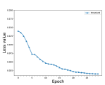
(a) Emotion6

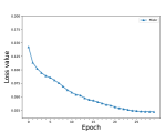
(b) Flickr-LDL

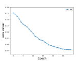
(c) RAF-LDL

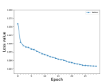
(d) Twitter-LDL

Figure 4: Convergence on various datasets.

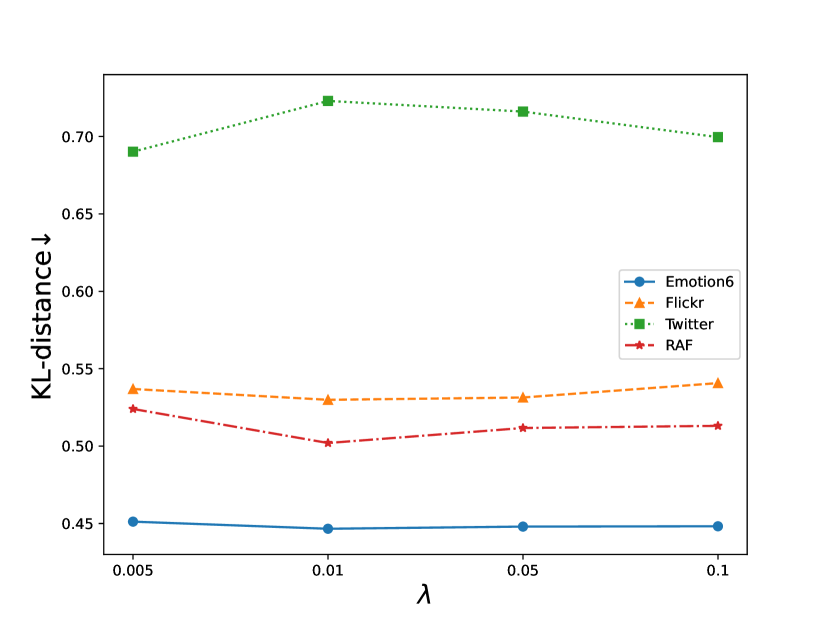
(a) KL with varying $\lambda$

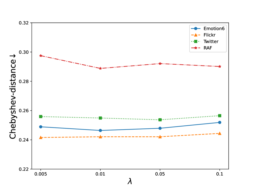
(b) Chebyshev with varying $\lambda$

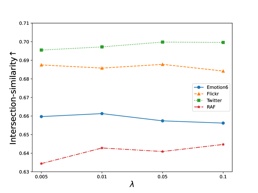
(c) Intersection with varying $\lambda$

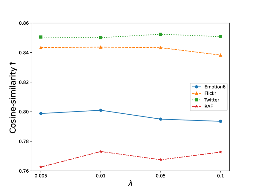
(d) Cosine with varying $\lambda$

Figure 5: Convergence on (a) Emotion6, (b) Flickr-LDL, (c) RAF-LDL and (d) Twitter-LDL.

3.6.3 Ablation Study

Our ablation study dissected the contributions of the PRR loss and unsupervised consistency loss to RankMatch’s effectiveness. Initially, the model was pre-trained using only 10% of the labeled data to establish a baseline performance. The results of this stage demonstrated the capability of the model to learn from a limited amount of data. Subsequently, the ranking loss was incorporated into the training process, utilizing the same 10% of labeled data. In the final stage, the model was augmented with the unsupervised consistency loss, applied to the unlabeled data. This step built upon the pre-trained model with the supervised ranking loss. Ablation experiment results are shown in Table. 3. From this, we can draw the following conclusions:

(a) The PRR loss resulted in a significant improvement over the baseline, emphasizing the component’s effectiveness in enhancing the model’s discriminative ability, even with limited labeled data. This enhancement accentuates the importance of the ranking mechanism in capturing the complex relationships between labels within a semi-supervised framework.

(b) The unsupervised consistency loss led to further gains, as demonstrated by the substantial increase in performance presented in the third row of the ablation table. This indicates that the unsupervised loss plays a vital role in harnessing the unlabeled data and refining the model’s predictions.

3.6.4 Convergence Analysis

In this section, we conduct a convergence analysis of the RankMatch algorithm. The experimental results are shown in Fig. 4. The following conclusions are drawn from the observed loss trajectories during training epochs: For Emotion6, a precipitous decline in loss values during initial epochs underscores the model’s rapid learning rate, which then transitions into a stable phase, indicating a quick adjustment to the dataset specifics. Flickr-LDL mirrors the quick learning pattern of Emotion6 but stabilizes sooner, hinting at an even faster rate of convergence, which could be a characteristic of the dataset or an indication of the model’s proficiency in learning. The loss values for RAF-LDL decrease more gradually, reflecting a consistent and methodical learning process, indicative of the model’s steady performance improvement over time. Twitter-LDL demonstrates a steady downward trend in loss, akin to RAF-LDL, highlighting the model’s consistent learning curve across varying datasets. Overall, the uniform reduction in loss values across datasets emphasizes the RankMatch algorithm’s capability to optimize the loss function effectively, thereby potentially enhancing the model’s prediction accuracy as training advances.

3.6.5 Parameter Sensitivity Analysis

In the parameter sensitivity analysis section, we examine the impact of the hyperparameter $\lambda$ on the performance of our semi-supervised label distribution learning algorithm across four different datasets. The results of the parameter analysis are shown in Fig. 5. From Fig. 5, we can draw the following conclusions: (a)For the KL divergence, the performance remains relatively stable across different values of $\lambda$ on all datasets. (b)The Chebyshev distance metric shows a mild upward trend as $\lambda$ increases for the Emotion6 and RAF-LDL datasets. However, this trend is not observed for the Flickr-LDL and Twitter-LDL datasets. (c)Intersection similarity presents a clear trend where performance improves with increasing $\lambda$ on the Emotion6 dataset, but remains relatively stable on the RAF-LDL and Twitter-LDL datasets. The Flickr-LDL dataset shows a slight decline in performance as $\lambda$ increases. (d)The Cosine similarity metric demonstrates robustness to changes in $\lambda$ across all datasets.

The parameter $\lambda$ has a variable impact on different metrics and datasets. In cases where the performance is affected, the changes are generally gradual and not abrupt, indicating that the RankMatch algorithm is not highly sensitive to this parameter. This implying that the method is robust to parameter changes and can maintain consistent performance without requiring fine-tuned parameter settings.

emotion6	Can $\downarrow$	Che $\downarrow$	Clark $\downarrow$	Cos $\uparrow$	Inter$\uparrow$	KL $\downarrow$
$\lambda$ =0.01 t = 0.1	3.445	0.2419	1.537	0.8037	0.6658	0.4319
$\lambda$ =0.01 t = 0.2	3.446	0.2485	1.542	0.7977	0.6628	0.4491
$\lambda$ =0.01 t = 0.3	3.484	0.2506	1.55	0.7933	0.6554	0.4519
$\lambda$ =0.01 t = 0.4	3.42	0.2447	1.535	0.8067	0.6631	0.4302
RAF-LDL	Can $\downarrow$	Che $\downarrow$	Clark $\downarrow$	Cos $\uparrow$	Intern $\uparrow$	KL $\downarrow$
$\lambda$ =0.01 t = 0.1	3.086	0.2954	1.467	0.7628	0.6351	0.517
$\lambda$ =0.01 t = 0.2	3.053	0.2897	1.457	0.7726	0.6428	0.4954
$\lambda$ =0.01 t = 0.3	3.081	0.2956	1.469	0.7643	0.6382	0.5114
$\lambda$ =0.01 t = 0.4	3.103	0.2982	1.476	0.7612	0.6345	0.5226

Table 4: Impact of Threshold t on the Performance of the RankMatch.

3.6.6 Impact of Threshold t on Experimental Results

The influence of the threshold tin the Pairwise Relevance Ranking loss is critical in determining the sensitivity of the RankMatch algorithm to label ranking discrepancies. Our experiments, as detailed in Table 4, investigate this impact across various datasets and metrics. We observe that the performance metrics on Canberra and Chebyshev distances maintain a relative stability across different tvalues, suggesting that the PRR loss is robust to the threshold variations. The Clark and Cosine distances exhibit a trend where a larger t marginally improves model performance, hinting at the algorithm’s enhanced ability to discern more significant label relationships.

Particularly noteworthy is the trend in intersection similarity and KL divergence metrics, especially for the Emotion6 dataset, where a higher threshold t correlates with improved alignment to ground truth labels. This suggests that a careful calibration of t can leverage the RankMatch algorithm’s strength in datasets with complex label semantics. The results emphasize the need for a balanced threshold that can effectively distinguish meaningful label importance differences, especially under the constraints of limited labeled data in a semi-supervised learning setting.

4 Conclusion

RankMatch advances SSLDL by efficiently combining limited labeled data with a larger volume of unlabeled examples, thus reducing the dependency on extensive manual annotations. It incorporates an averaging strategy inspired by ensemble learning and a pairwise relevance ranking loss, which together enhance prediction stability and model robustness. Our experimental validations across multiple datasets establish RankMatch as a superior method, validating its effectiveness in SSLDL applications.

References

- Basak & Yin (2023) Basak, H. and Yin, Z. Pseudo-label guided contrastive learning for semi-supervised medical image segmentation. In IEEE/CVF Conference on Computer Vision and Pattern Recognition, CVPR 2023, Vancouver, BC, Canada, June 17-24, 2023, pp. 19786–19797. IEEE, 2023.
- Borth et al. (2013) Borth, D., Ji, R., Chen, T., Breuel, T., and Chang, S.-F. Large-scale visual sentiment ontology and detectors using adjective noun pairs. In Proceedings of the 21st ACM international conference on Multimedia, pp. 223–232, 2013.
- Carroll & Russell (1996) Carroll, J. M. and Russell, J. A. Do facial expressions signal specific emotions? judging emotion from the face in context. Journal of personality and social psychology, 70(2):205, 1996.
- Chen et al. (2020) Chen, S., Wang, J., Chen, Y., Shi, Z., Geng, X., and Rui, Y. Label distribution learning on auxiliary label space graphs for facial expression recognition. In 2020 IEEE/CVF Conference on Computer Vision and Pattern Recognition, CVPR 2020, Seattle, WA, USA, June 13-19, 2020, pp. 13981–13990. Computer Vision Foundation / IEEE, 2020. doi: 10.1109/CVPR42600.2020.01400.
- Chen et al. (2021) Chen, X., Yuan, Y., Zeng, G., and Wang, J. Semi-supervised semantic segmentation with cross pseudo supervision. In IEEE Conference on Computer Vision and Pattern Recognition, CVPR 2021, virtual, June 19-25, 2021, pp. 2613–2622. Computer Vision Foundation / IEEE, 2021.
- Cole et al. (2021) Cole, E., Mac Aodha, O., Lorieul, T., Perona, P., Morris, D., and Jojic, N. Multi-label learning from single positive labels. In Proceedings of the IEEE/CVF Conference on Computer Vision and Pattern Recognition, pp. 933–942, 2021.
- Cubuk et al. (2020) Cubuk, E. D., Zoph, B., Shlens, J., and Le, Q. V. Randaugment: Practical automated data augmentation with a reduced search space. In Proceedings of the IEEE/CVF conference on computer vision and pattern recognition workshops, pp. 702–703, 2020.
- DeVries & Taylor (2017) DeVries, T. and Taylor, G. W. Improved regularization of convolutional neural networks with cutout. arXiv preprint arXiv:1708.04552, 2017.
- Fini et al. (2023) Fini, E., Astolfi, P., Alahari, K., Alameda-Pineda, X., Mairal, J., Nabi, M., and Ricci, E. Semi-supervised learning made simple with self-supervised clustering. In IEEE/CVF Conference on Computer Vision and Pattern Recognition, CVPR 2023, Vancouver, BC, Canada, June 17-24, 2023, pp. 3187–3197. IEEE, 2023.
- Gao et al. (2017) Gao, B.-B., Xing, C., Xie, C.-W., Wu, J., and Geng, X. Deep label distribution learning with label ambiguity. IEEE Transactions on Image Processing, 26(6):2825–2838, 2017.
- Geng (2016) Geng, X. Label distribution learning. IEEE Trans. Knowl Data Eng, 28(7):1734–1748, 2016.
- Geng et al. (2013) Geng, X., Yin, C., and Zhou, Z.-H. Facial age estimation by learning from label distributions. IEEE transactions on pattern analysis and machine intelligence, 35(10):2401–2412, 2013.
- González et al. (2021) González, M., González-Almagro, G., Triguero, I., Cano, J.-R., and García, S. Decomposition-fusion for label distribution learning. Information Fusion, 66:64–75, 2021.
- Hannan et al. (2021) Hannan, M. A., How, D. N., Mansor, M. B., Lipu, M. S. H., Ker, P. J., and Muttaqi, K. M. State-of-charge estimation of li-ion battery using gated recurrent unit with one-cycle learning rate policy. IEEE Transactions on Industry Applications, 57(3):2964–2971, 2021.
- He et al. (2016) He, K., Zhang, X., Ren, S., and Sun, J. Deep residual learning for image recognition. In Proceedings of the IEEE conference on computer vision and pattern recognition, pp. 770–778, 2016.
- Hershey & Olsen (2007) Hershey, J. R. and Olsen, P. A. Approximating the kullback leibler divergence between gaussian mixture models. In 2007 IEEE International Conference on Acoustics, Speech and Signal Processing-ICASSP’07, volume 4, pp. IV–317. IEEE, 2007.
- Hou et al. (2017) Hou, P., Geng, X., Huo, Z.-W., and Lv, J.-Q. Semi-supervised adaptive label distribution learning for facial age estimation. In Thirty-First AAAI Conference on Artificial Intelligence, 2017.
- Jang et al. (2016) Jang, E., Gu, S., and Poole, B. Categorical reparameterization with gumbel-softmax. arXiv preprint arXiv:1611.01144, 2016.
- Jia et al. (2018) Jia, X., Li, W., Liu, J., and Zhang, Y. Label distribution learning by exploiting label correlations. In Pro. Conf. Artif. Intell., volume 32, 2018.
- Jia et al. (2019) Jia, X., Li, Z., Zheng, X., Li, W., and Huang, S.-J. Label distribution learning with label correlations on local samples. IEEE Transactions on Knowledge and Data Engineering, 33(4):1619–1631, 2019.
- Jia et al. (2021a) Jia, X., Shen, X., Li, W., Lu, Y., and Zhu, J. Label distribution learning by maintaining label ranking relation. IEEE Transactions on Knowledge and Data Engineering, 2021a.
- Jia et al. (2021b) Jia, X., Wen, T., Ding, W., Li, H., and Li, W. Semi-supervised label distribution learning via projection graph embedding. Information Sciences, 581:840–855, 2021b.
- Jia et al. (2023) Jia, X., Shen, X., Li, W., Lu, Y., and Zhu, J. Label distribution learning by maintaining label ranking relation. IEEE Trans. Knowl. Data Eng., 35(2):1695–1707, 2023.
- Jiang et al. (2022) Jiang, Y., Li, X., Chen, Y., He, Y., Xu, Q., Yang, Z., Cao, X., and Huang, Q. Maxmatch: Semi-supervised learning with worst-case consistency. IEEE Transactions on Pattern Analysis and Machine Intelligence, 45(5):5970–5987, 2022.
- Jiang et al. (2023) Jiang, Y., Li, X., Chen, Y., He, Y., Xu, Q., Yang, Z., Cao, X., and Huang, Q. Maxmatch: Semi-supervised learning with worst-case consistency. IEEE Trans. Pattern Anal. Mach. Intell., 45(5):5970–5987, 2023.
- Klinker (2011) Klinker, F. Exponential moving average versus moving exponential average. Mathematische Semesterberichte, 58:97–107, 2011.
- Krizhevsky et al. (2012) Krizhevsky, A., Sutskever, I., and Hinton, G. E. Imagenet classification with deep convolutional neural networks. Advances in neural information processing systems, 25, 2012.
- Li & Deng (2019) Li, S. and Deng, W. Blended emotion in-the-wild: Multi-label facial expression recognition using crowdsourced annotations and deep locality feature learning. International Journal of Computer Vision, 127(6-7):884–906, 2019.
- Ling & Geng (2019) Ling, M. and Geng, X. Indoor crowd counting by mixture of gaussians label distribution learning. IEEE Transactions on Image Processing, 28(11):5691–5701, 2019.
- Liu et al. (2022) Liu, X., Zhu, J., Zheng, Q., Tian, Z., and Li, Z. Semi-supervised label distribution learning with co-regularization. Neurocomputing, 491:353–364, 2022.
- Liu et al. (2019) Liu, Z., Chen, Z., Bai, J., Li, S., and Lian, S. Facial pose estimation by deep learning from label distributions. In 2019 IEEE/CVF International Conference on Computer Vision Workshops, ICCV Workshops 2019, Seoul, Korea (South), October 27-28, 2019, pp. 1232–1240. IEEE, 2019.
- Morrison et al. (2018) Morrison, S. M., Pan, F., Gagné, O. C., Prabhu, A., Eleish, A., Fox, P. A., Downs, R. T., Bristow, T. F., Rampe, E. B., Blake, D. F., Vaniman, D. T., Achilles, C. N., Ming, D. W., Yen, A. S., Treiman, A. H., Morris, R. V., Chipera, S. J., Craig, P. I., Tu, V., Castle, N., Sarrazin, P. C., Marais, D. J. D., and Hazen, R. M. Predicting multi-component mineral compositions in gale crater, mars with label distribution learning. 2018.
- Peng et al. (2015) Peng, K.-C., Chen, T., Sadovnik, A., and Gallagher, A. C. A mixed bag of emotions: Model, predict, and transfer emotion distributions. In Proceedings of the IEEE conference on computer vision and pattern recognition, pp. 860–868, 2015.
- Shen et al. (2017) Shen, W., Zhao, K., Guo, Y., and Yuille, A. L. Label distribution learning forests. Advances in neural information processing systems, 30, 2017.
- Shih et al. (2008) Shih, F. Y., Chuang, C.-F., and Wang, P. S. Performance comparisons of facial expression recognition in jaffe database. International Journal of Pattern Recognition and Artificial Intelligence, 22(03):445–459, 2008.
- Sohn et al. (2020) Sohn, K., Berthelot, D., Carlini, N., Zhang, Z., Zhang, H., Raffel, C. A., Cubuk, E. D., Kurakin, A., and Li, C.-L. Fixmatch: Simplifying semi-supervised learning with consistency and confidence. Advances in neural information processing systems, 33:596–608, 2020.
- Wu et al. (2019) Wu, X., Wen, N., Liang, J., Lai, Y., She, D., Cheng, M., and Yang, J. Joint acne image grading and counting via label distribution learning. In 2019 IEEE/CVF International Conference on Computer Vision, ICCV 2019, Seoul, Korea (South), October 27 - November 2, 2019, pp. 10641–10650. IEEE, 2019.
- Xu et al. (2023) Xu, H., Liu, X., Zhao, Q., Ma, Y., Yan, C., and Dai, F. Gaussian label distribution learning for spherical image object detection. In Proceedings of the IEEE/CVF Conference on Computer Vision and Pattern Recognition, pp. 1033–1042, 2023.
- Xu & Zhou (2017) Xu, M. and Zhou, Z.-H. Incomplete label distribution learning. In Proc. Int. Joint Conf. Artif. Intell, pp. 3175–3181, 2017.
- Yang et al. (2017) Yang, J., Sun, M., and Sun, X. Learning visual sentiment distributions via augmented conditional probability neural network. In Proceedings of the AAAI Conference on Artificial Intelligence, volume 31, 2017.
- Yang et al. (2022) Yang, X., Song, Z., King, I., and Xu, Z. A survey on deep semi-supervised learning. IEEE Transactions on Knowledge and Data Engineering, 2022.
- You et al. (2019) You, Y., Li, J., Reddi, S., Hseu, J., Kumar, S., Bhojanapalli, S., Song, X., Demmel, J., Keutzer, K., and Hsieh, C.-J. Large batch optimization for deep learning: Training bert in 76 minutes. arXiv preprint arXiv:1904.00962, 2019.
- Zhang et al. (2021) Zhang, B., Wang, Y., Hou, W., Wu, H., Wang, J., Okumura, M., and Shinozaki, T. Flexmatch: Boosting semi-supervised learning with curriculum pseudo labeling. Advances in Neural Information Processing Systems, 34:18408–18419, 2021.
- Zhang & Zhou (2014) Zhang, M. and Zhou, Z. A review on multi-label learning algorithms. IEEE Trans. Knowl. Data Eng., 26(8):1819–1837, 2014. doi: 10.1109/TKDE.2013.39. URL https://doi.org/10.1109/TKDE.2013.39.
- Zhou et al. (2020) Zhou, X., Wei, Z., Xu, M., Qu, S., and Guo, G. Facial depression recognition by deep joint label distribution and metric learning. IEEE Transactions on Affective Computing, 13(3):1605–1618, 2020.
- Zhou & Zhou (2021) Zhou, Z.-H. and Zhou, Z.-H. Ensemble learning. Springer, 2021.