The Hubble Deep Hydrogen Alpha (HDH$\alpha$) Project: I. Catalog of Emission-line Galaxies

Abstract

We present the first results of the Hubble Deep Hydrogen Alpha (HDH$\alpha$) project, which analyzes the space-borne deep H$\alpha$ narrowband imaging data in the GOODS-S region. The HDH$\alpha$ data comprises 72 orbits’ images taken with the HST ACS/WFC F658N filter. The exposure time varies across a total area of $\sim$76.1 $\rm{arcmin}^{2}$, adding up to a total exposure time of 195.7 ks, among which 68.8 ks are spent in the deepest region. These images are aligned, reprojected, and combined to have the same pixel grid as the Hubble Legacy Fields (HLF). The scientific goals of the HDH$\alpha$ include establishing a sample of emission-line galaxies (ELGs) including [O iii] emitters at $z\sim$ 0.3, [O ii] emitters at $z\sim$ 0.8, and Lyman-$\alpha$ emitters (LAEs) at $z\sim 4.4$, studying the line morphology of ELGs with high resolution imaging data, and statistically analyzing the line luminosity functions and line equivalent-width distributions of ELGs selected with HST. Furthermore, the HDH$\alpha$ project enhances the legacy value of the GOODS-S field by contributing the first HST-based narrowband image to the existing data sets, which includes the HST broadband data and other ancillary data from X-ray to radio taken by other facilities. In this paper, we describe the data reduction process of the HDH$\alpha$, select ELGs based on HST’s F658N and broadband data, validate the redshifts of the selected candidates by cross matching with the public spectroscopic catalogs in the GOODS-S, and present a final catalog of the confirmed [O iii] emitters at $z\sim$ 0.3, [O ii] emitters at $z\sim$ 0.8, and LAEs at $z\sim 4.4$.

1 Introduction

Distant galaxies are essential for our understanding of the early Universe and the formation and evolution of galaxies. In the optical band, there are two techniques widely used to search for and study high redshift galaxies, which are the Lyman break technique and the emission line excess technique. The former technique, also called the drop-out technique (Steidel et al., 1996), selects high-$z$ galaxies via their rest-frame UV break features in series broadband images, caused by the absorption of neutral hydrogen within the galaxies and in the intergalactic medium (IGM). The latter technique identifies galaxies with a strong emission line at a particular redshift, where the central wavelength of the emission line is redshifted in the bandpass of the narrowband filter, causing a flux excess in the narrowband over the corresponding broadband. This method identifies high redshift galaxies based on their strong Lyman-$\alpha$ emission line, which was predicted as a promising tracer of high redshift galaxies in the 1960s (Partridge & Peebles, 1967). However, this technique did not succeed until the middle 1990s when better CCD detectors with larger field-of-view (FOV), larger telescopes, and better narrowband filters were available (Cowie & Hu, 1998; Rhoads et al., 2000).

Over the past two decades, the drop-out technique has been widely used to select high redshift star-forming galaxies with deep broadband images from numerous survey campaigns, especially with the Hubble Space Telescope (HST). With the images taken in the first deep blank field, the Hubble Deep Field (Williams et al., 1996), galaxies at $z\sim 4$ were selected successfully to study cosmic star formation history (Madau et al., 1996). Using the deep mosaics based on images delivered by the Great Observatories Origins Deep Survey (GOODS, Giavalisco et al., 2004) and Hubble Ultra Deep Field program (HUDF, Beckwith et al., 2006), the redshift limit had been pushed to $z\sim 6$ (Bouwens et al., 2004; Dickinson et al., 2004; Bouwens et al., 2006). Even a handful of galaxies at $z\sim 7$ have been identified with additional HST/NICMOS and ground-based (e.g., $VLT$/ISAAC, $Subaru$/MOIRCS) observations (Bouwens et al., 2008). Further breakthroughs in the search of high-$z$ galaxies were accomplished using the Wide Field Camera 3 Infrared Channel (WFC3/IR). New generation surveys taken with the WFC3/IR, including the HUDF09 (Bouwens et al., 2011), the Cosmic Assembly Near-infrared Deep Extragalactic Legacy Survey (CANDELS, Grogin et al., 2011; Koekemoer et al., 2011), the Early Release Science program of WFC3 (ERS, Windhorst et al., 2011), and the HUDF12 (Koekemoer et al., 2013), had enabled the discovery of galaxies up to $z\simeq 8-10$ (Bouwens et al., 2010; Oesch et al., 2013, 2014; Bouwens et al., 2015). Recently, the HST surveys of gravitational lensing galaxy clusters have provided a new way to search for high $z$ galaxies (e.g. the Hubble Frontier Field, Lotz et al., 2017), which used galaxy clusters as a natural telescope to search and study high-$z$ galaxies (McLeod et al., 2016; Ishigaki et al., 2018; Bouwens et al., 2022).

Unlike the tremendously successful broadband drop-out surveys with HST as mentioned above, emission-line surveys using narrowband selection technique are mainly carried out with ground-based telescopes, e.g., the Subaru/XMM-Newton Deep Survey (SXDS, Ouchi et al., 2008), the Lyman Alpha Galaxies in the Epoch of Reionization Survey (LAGER, Zheng et al., 2017), the Subaru SILVERRUSH survey (Ouchi et al., 2018), and the upcoming Javalambre-Physics of the Accelerated Universe Astrophysical Survey (J-PAS, Benitez et al., 2014). A wide range of research topics on Lyman-$\alpha$ Emitters (LAEs) had been probed based on the narrowband imaging technique, including diffuse Lyman-$\alpha$ halos (e.g. Momose et al., 2014, 2016), giant diffuse Lyman-$\alpha$ nebulae (Cantalupo et al., 2014; Hennawi et al., 2015; Cai et al., 2017a; Arrigoni Battaia et al., 2018), overdense regions such as protoclusters and large scale structures at high redshifts (Zheng et al., 2016; Cai et al., 2017b; Jiang et al., 2018; Hu et al., 2021; Zheng et al., 2021), and the ionization state of the cosmic reionization epoch (Malhotra & Rhoads, 2002; Ouchi et al., 2010; Kashikawa et al., 2011; Zheng et al., 2017; Hu et al., 2019; Wold et al., 2021). Moreover, this technique has also been used to search for other emission-line emitters to constrain the line luminosity functions and the cosmic star formation rate densities at $z\lesssim 2$.(Sobral et al., 2013; Hayashi et al., 2018; Khostovan et al., 2020).

With HST, narrowband imaging surveys for high-$z$ galaxies are rare. Most of HST’s narrowband imaging surveys were targeted at local galaxies and objects, e.g., local ultra-faint dwarf galaxies (Fu et al., 2021), young stellar objects (Ferreras et al., 2009), and supernova remnants (i.e., SN1987A, Larsson et al., 2013) in the Large Magellanic Cloud. In the high-$z$ Universe, only a few of HST’s narrowband surveys were reported. In the Ly$\alpha$ morphological studies of high-$z$ LAEs, Bond et al. (2010) reported compact Ly$\alpha$ emission of LAEs at $z\sim$ 3.1 with the WFPC2 narrowband observations, while Finkelstein et al. (2011) detected the resolved Ly$\alpha$ emission from two out of three LAEs at $z\sim 4.4$ with the ACS/WFC narrowband observations. Decarli et al. (2012) used the WFC3/UVIS narrowband observations to search for the extended Ly$\alpha$ emission around two quasars at $z>6$, while neither extended Ly$\alpha$ emission around quasars nor LAE companions were found.

Here we introduce the Hubble Deep Hydrogen Alpha (HDH$\alpha$) project, which is based on the deepest HST/ACS H$\alpha$ narrowband (F658N) imaging survey data and is also the largest and deepest narrowband imaging survey in the blank field taken with HST. The final HDH$\alpha$ image, covering part of the GOODS-S Field, allows a systematic search for sources with strong emission lines along with deep broadband images at HST’s spatial resolution. With this sample, we can further analyze the emission-line galaxies’ morphology and spectral energy distribution in the GOODS-S field with the most up-to-date Hubble Legacy Field (HLF: Illingworth et al., 2016, Illingworth et al. in prep.) data.

The structure of the paper is as follows. In Section 2, we describe the observations of the narrowband imaging surveys with HST (§ 2.1), the HDH$\alpha$ project (§ 2.2), the reduction process of the HDH$\alpha$ narrowband data (§ 2.3), and the data quality of the mosaic HDH$\alpha$ image (§ 2.4). In Section 3, we discuss the photometry of HDH$\alpha$ sources. We select emission-line galaxies (ELGs), including [O iii] emitters at $z\sim 0.3$, [O ii] emitters at $z\sim 0.8$, and LAEs at $z\sim 4.4$ with the HDH$\alpha$ narrowband image and the HLF broadband images in Section 4. Finally, we summarize our main results in Section 5. Throughout this paper, we adopt a standard cosmology model with parameters $\Omega_{M}=0.3$, $\Omega_{\Lambda}=0.7$, $H_{0}=\rm{70\ km\ s^{-1}Mpc^{-1}}$. All magnitudes throughout this paper are given in the AB system (Oke & Gunn, 1983).

2 HST Narrowband Surveys and Data Reduction

2.1 Deep Narrowband Imaging Surveys with HST

We search for the HST’s narrowband imaging surveys in extragalactic fields with the planned and archived exposures catalog (PAEC, version: 2021-12-01), which summarizes all exposures taken or planned with HST since Cycle 7. We use HEALPix (Hierarchical Equal Area isoLatitude Pixelation, its python wrapper: healpy, see Górski et al., 2005; Zonca et al., 2019) to divide the celestial sphere into a series of cells with equal areas and calculate the sum of the exposure time of narrowband observations in each cell. The healpy’s parameter $N_{\textrm{Side}}$ is set to $N_{\textrm{Side}}$ = 128, corresponding to an area of each cell of 755 $\rm arcmin^{2}$.

We check the narrowband imaging surveys taken with HST’s WFPC2, ACS/WFC, WFC3/UVIS, and WFC3/IR using HEALPix. The deepest exposures of a single narrowband filter taken with these cameras are summarized in Tab. 1. We find that the ACS/WFC has the deepest narrowband (F658N) exposure in GOODS-S, which is a famous extragalactic blank field. Other deep narrowband surveys in Tab. 1 are targeted at nearby objects, thus unsuitable for the extragalactic study. Therefore, we do not carry out further reductions to these data sets in this study.

Table 1: The deepest narrowband imaging surveys for each of the HST imaging cameras

Camera	Deepest Region	Narrowband Filters	Program Exposure Time
			(Second)
ACS/WFC	R.A.$=03^{h}32^{m}20.62^{s}$, Dec.$=-27^{d}57^{m}11.47^{s}$	F658N	197122
	GOODS-S
WFC3/UVIS	R.A.$=00^{h}25^{m}42.86^{s}$, Dec.$=-72^{d}01^{m}03.45^{s}$	F502N	138186
	47 Tuc
WFPC2	R.A.$=05^{h}37^{m}30^{s}$, Dec.$=-69^{d}25^{m}21.16^{s}$	F656N	125990
	LMC
WFC3/IR	R.A. $=10^{h}38^{m}22.33^{s}$, Dec.$=-58^{d}09^{m}37.33^{s}$	F167N	66291
	G286.21+0.17

2.2 HDH$\alpha$: The HST ACS/WFC F658N Imaging Survey in GOODS-S

The F658N narrowband filter is one of the 16 filters onboard the Wide Field Channel (WFC) of HST/ACS. The F658N filter is described as a H$\alpha$ filter with a central wavelength of 6584Å and a full width at half maximum (FWHM) of 87Å, respectively. The system throughput of HSTACS/WFC F658N, along with broadband filters F435W, F606W, F775W and F814W, is presented in Fig. 1.

The HDH$\alpha$ is located in the GOODS-S field. The narrowband images were collected as parallel observations during the ERS program (Program ID: 11359, PI: Robert O’Connell, Windhorst et al., 2011). The F658N imaging of the HDH$\alpha$ is composed of 8 independent pointings, each of which includes a 9-orbit ACS/WFC F658N observation. It covers a total area of 86 arcmin² in the GOODS-S region. The total exposure time of the HDH$\alpha$ is 197.1 ks, and the deepest region with 68.8 ks. The key parameters of the HDH$\alpha$ project are summarized in Tab. 2.

The narrowband data of the HDH$\alpha$ was probed partially by Finkelstein et al. (2011) to study the Ly$\alpha$ morphology of three LAEs at $z\sim 4.4$. However, such narrowband data has never been combined and released as a unified data set. In contrast, the broadband images in this field had been reduced and released by previous programs (e.g., GOODS and HLF; Giavalisco et al., 2004; Illingworth et al., 2016, Illingworth et al. in prep.). Therefore, a fully reduced narrowband image in this field will increase the legacy value of the GOODS-S field. The footprints of the HDH$\alpha$ project, as well as other large imaging and spectroscopic surveys in the GOODS-S region, are presented in Fig. 2.

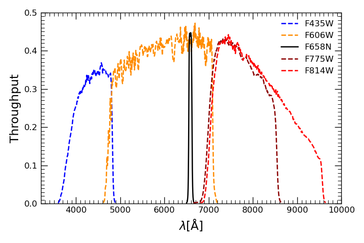
Figure 1: System throughputs of the broadband filters F435W, F606W, F775W, F814W, and the narrowband filter F658N of HST ACS/WFC.

Table 2: The Summary of the HDH$\alpha$ Project

Parameter	Value
Position(J2000)	R.A.$=03^{h}32^{m}33^{s}$, Dec$=-27^{\circ}48^{\prime}52\arcsec$
Area	86 arcmin2 (76.1a arcmin2 )
Camera and Filter	HSTACS/WFC F658N
Number of Exposures	214 (212b)
Total Exposure Time	197,122s (195,690sb)
Number of Orbits	72
$5\sigma$ Depth	m${}_{\textrm{F658N}}(5\sigma)$ = 25.4 - 25.8 mag

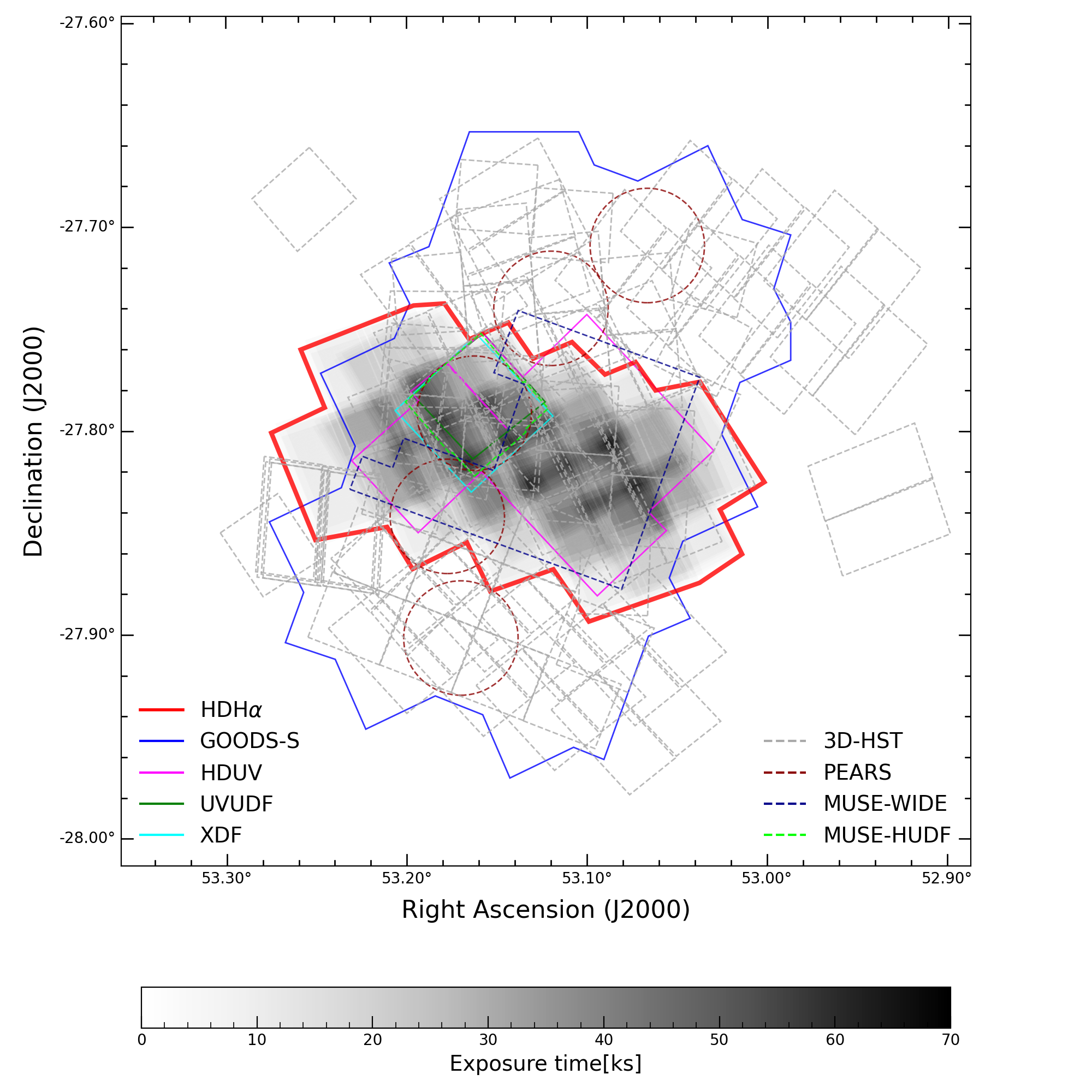
Figure 2: The exposure time map of the HDH$\alpha$ and the footprints of other imaging and spectroscopic surveys. The depth of the exposure time map is encoded by the color bar at the bottom. The solid line shows the coverage of broadband imaging surveys such as the GOODS-S (Giavalisco et al., 2004), the Hubble Deep UV Legacy Survey (HDUV, Oesch et al., 2018), Hubble Ultraviolet Ultra Deep Field (UVUDF, Teplitz et al., 2013), the Hubble eXtreme Deep Field (XDF, Illingworth et al., 2013), and our narrowband project the HDH$\alpha$. The dashed lines demonstrate the coverages and the pointings of three spectroscopic surveys, i.e., the 3D-HST (Brammer et al., 2012; Momcheva et al., 2016), the Probing Evolution And the Reionization Spectroscopically (PEARS) program (Pirzkal et al., 2013), the MUSE-Wide (Urrutia et al., 2019) and the MUSE Hubble Ultra Deep Field surveys (MUSE-HUDF, Bacon et al., 2022).

2.3 HST’s Narrowband Image Processing

2.3.1 Data acquisition

We obtain the calibrated HDH$\alpha$ images from Mikulski Archive for Space Telescopes (MAST). These images have been calibrated with the ACS pipeline calacs, whose function is briefly summarized here. The calibration pipeline starts with raw exposures and initially flags bad pixels in the data quality array from a known bad pixel table. Then, bias images and bias levels determined from overscan regions are subtracted. In this step, the bias shift, cross-talk, and striping are also corrected for the full frame ACS/WFC images. After this, the charge transfer efficiency (CTE) degradation is corrected, followed by cosmic ray identification. Lastly, the dark frame subtraction and the flat field correction are carried out.

We then inspect the quality of the downloaded data visually. Bad quality regions are then masked out. In addition, we check two keywords, QUALITY and EXPFLAG, in the image header of the individual frame for the guide star acquisition failure problem. All these images pass that check.

2.3.2 Narrowband Image Registration

Due to the positional uncertainties of guide stars acquired during HST’s observations, the World Coordinate System (WCS) of the narrowband images needs to be refined for a precise registration across all images in our data set. Furthermore, as there are quite a few bright sources but many cosmic rays in an individual narrowband image taken with HST, it is quite difficult to align these images directly. Here we follow the alignment method introduced by Mack (2015), in which a set of WFC3 narrowband images of Messier 16 were aligned and combined to overcome the alignment problem in the HDH$\alpha$.

Our registration procedure begins with drizzling the narrowband images in the same visit and then works on the visit-based narrowband images for further alignment and combination. We use DrizzlePac, a suite of tasks including AstroDrizzle, TweakReg and, Tweakback for aligning, distortion-correcting, cosmic-ray cleaning, and combining HST images. We first combine the individual exposure images within the same visit to obtain a cosmic-ray cleaned, relatively deep image with AstroDrizzle (version 3.3.0, Gonzaga et al., 2012). Then we use the SExtractor (version 2.19.5, Bertin & Arnouts, 1996) to identify the sources and create a catalog for each visit-based image. We cross match our catalog with the reference catalog, which contains bright sources ($\textrm{F606W}<$ 23.5 mag) from the HLF catalog (HLF, Whitaker et al., 2019). This step is used to remove the residual cosmic rays for each visit. Then the WCS solutions for visit-based images are solved by the TweakReg (version 1.4.7) task, which is designed to improve the alignments of HST’s images. The WCS fitting results of each visit are shown in Tab. 3. Finally, these results are applied to the individual exposure image in each visit by the Tweakback (version 0.4.1) task.

The typical root-mean-square (RMS) value of the alignment residual for visit-based images is $\sim$ 0.3 pixels (Tab. 3). Although it is larger than the value recommended by the ACS data handbook ($\sim$ 0.1 pixels), our WCS solution is based on tens of bright sources ($\simeq 10-20$), which is similar to the case of the 3D-HST infrared image (RMS $\sim$ 0.4 pixels for WFC3/IR $F160W$ images, Skelton et al., 2014). We reject one visit’s data with only two exposures due to a poor WCS solution.

Table 3: The WCS fitting results of individual visits of the HDH$\alpha$.

Visit	Pointing Position	Number of	Total Time of	ShiftX	ShiftY	RMSX	RMSY	Number of
ID		Exposures	Exposures					Matched Sources
			(second)	(pixel)	(pixel)	(pixel)	(pixel)
01	$03^{h}32^{m}46.07^{s}-27^{d}46^{m}33.98^{s}$	12	8802.0	0.96	-2.32	0.36	0.39	18
02	$03^{h}32^{m}37.58^{s}-27^{d}47^{m}07.84^{s}$	12	8802.0	-0.47	-0.93	0.23	0.38	11
03	$03^{h}32^{m}29.09^{s}-27^{d}47^{m}42.19^{s}$	12	8802.0	-1.41	-2.29	0.23	0.15	16
04	$03^{h}32^{m}20.66^{s}-27^{d}48^{m}17.36^{s}$	12	8802.0	-0.12	2.43	0.40	0.35	16
05	$03^{h}32^{m}12.07^{s}-27^{d}48^{m}52.21^{s}$	12	8802.0	-0.46	-0.35	0.23	0.20	20
06	$03^{h}32^{m}48.92^{s}-27^{d}48^{m}31.08^{s}$	12	8802.0	-0.21	0.37	0.32	0.10	7
07	$03^{h}32^{m}40.38^{s}-27^{d}49^{m}05.69^{s}$	12	8802.0	-1.59	-1.25	0.17	0.44	13
09	$03^{h}32^{m}23.44^{s}-27^{d}50^{m}13.86^{s}$	12	8802.0	0.27	2.81	0.21	0.33	24
10	$03^{h}32^{m}14.82^{s}-27^{d}50^{m}49.56^{s}$	12	8802.0	-1.42	-3.28	0.16	0.28	11
11	$03^{h}32^{m}45.96^{s}-27^{d}46^{m}29.17^{s}$	3	2139.0	0.54	-3.02	0.23	0.19	8
12	$03^{h}32^{m}37.47^{s}-27^{d}47^{m}02.97^{s}$	3	2139.0	1.05	0.43	0.32	0.26	7
13	$03^{h}32^{m}28.99^{s}-27^{d}47^{m}37.37^{s}$	3	2139.0	0.08	0.22	0.14	0.27	12
14	$03^{h}32^{m}20.55^{s}-27^{d}48^{m}12.51^{s}$	3	2139.0	0.17	2.21	0.37	0.16	16
15	$03^{h}32^{m}11.97^{s}-27^{d}48^{m}47.36^{s}$	3	2139.0	-0.72	-0.59	0.13	0.17	16
16	$03^{h}32^{m}48.82^{s}-27^{d}48^{m}26.31^{s}$	3	2139.0	-0.12	0.63	0.20	0.29	8
17	$03^{h}32^{m}40.28^{s}-27^{d}49^{m}00.87^{s}$	3	2139.0	0.35	0.57	0.29	0.52	17
18	$03^{h}32^{m}31.75^{s}-27^{d}49^{m}33.94^{s}$	3	2139.0	-2.29	-6.48	0.33	0.14	6
19	$03^{h}32^{m}23.33^{s}-27^{d}50^{m}09.05^{s}$	3	2139.0	-0.57	0.04	0.18	0.13	16
20	$03^{h}32^{m}14.72^{s}-27^{d}50^{m}44.80^{s}$	3	2139.0	-0.80	-0.12	0.39	0.18	14
25	$03^{h}32^{m}50.89^{s}-27^{d}46^{m}32.94^{s}$	8	10964.0	1.07	1.64	0.37	0.30	9
26	$03^{h}32^{m}39.24^{s}-27^{d}47^{m}18.52^{s}$	8	10964.0	0.90	0.84	0.32	0.17	14
27	$03^{h}32^{m}27.53^{s}-27^{d}48^{m}04.40^{s}$	8	10964.0	0.37	-0.85	0.26	0.22	20
28	$03^{h}32^{m}15.79^{s}-27^{d}48^{m}50.95^{s}$	8	10964.0	0.02	-1.08	0.35	0.25	23
29	$03^{h}32^{m}54.82^{s}-27^{d}48^{m}59.81^{s}$	8	10964.0	-0.07	1.76	0.18	0.26	10
30	$03^{h}32^{m}43.22^{s}-27^{d}49^{m}43.76^{s}$	8	10964.0	-1.13	-8.73	0.27	0.26	15
31	$03^{h}32^{m}31.53^{s}-27^{d}50^{m}30.52^{s}$	8	10964.0	-0.24	-0.17	0.12	0.20	23
32	$03^{h}32^{m}19.75^{s}-27^{d}51^{m}16.53^{s}$	8	10964.0	-0.86	0.01	0.23	0.28	21
a8	$03^{h}32^{m}31.48^{s}-27^{d}49^{m}44.10^{s}$	3	2221.0	-1.81	-5.95	0.40	0.30	7
b8	$03^{h}32^{m}31.99^{s}-27^{d}49^{m}35.61^{s}$	4	2928.0	-0.79	-5.71	0.41	0.16	5
c8	$03^{h}32^{m}31.96^{s}-27^{d}49^{m}43.71^{s}$	3	2221.0	-3.47	-6.04	0.16	0.05	8

2.3.3 Combination

The last image processing step combines the well-aligned calibrated images into a final mosaic image. We use AstroDrizzle to drizzle and fine-tune all narrowband F658N images to the pixel grid of the HLF image. The final image has a size of 25000$\times$ 25000 pixels, is located in the GOODS-S field, and has a pixel scale of $0^{\prime\prime}.06$. This step’s final products of AstroDrizzle consist of a science image and a corresponding inverse-variance weight map.

We also generate the efficient exposure map, which encodes the total exposure time on each pixel, by resampling and combining the efficient exposure maps of different visits with Swarp (version 2.38.0, Bertin, 2010). The efficient exposure map of each visit is one type of weight map generated by AstroDrizzle.

2.4 Data Quality Check

To check the image quality of the HDH$\alpha$, we conduct tests on the point spread function (PSF), check the astrometry, and probe the distributions of the exposure time and the magnitude depth in this subsection.

2.4.1 PSF

The PSF is a basic parameter of an astronomical image. It is also essential for multi-band photometric measurements. To check the consistency of fluxes in different bands, we follow previous projects (e.g., 3D-HST, HLF; Skelton et al., 2014; Whitaker et al., 2019) to measure the empirical PSF (ePSF) of the narrowband F658N image of the HDH$\alpha$ and four broadband (F435W, F606W, F775W, F814W) images of the HLF, which are used together to search for emission-line galaxies in Section 4.

Following Skelton et al. (2014), we obtain the ePSF of each image by stacking unsaturated bright stars across the mosaic image. We describe the method briefly here. We select an initial sample of stars from the horizontal sequence on the plot of narrowband flux ratios at different aperture sizes as a function of the Kron aperture (Kron, 1980) magnitudes, shown in panel (a) of Fig. 3. This sample is visually inspected to exclude unsuitable objects, such as artifacts, stars affected by nearby neighbors or cosmic rays. The number of usable stars varies by band, ranging from a minimum of 31 in F658N to a maximum of 162 in F606W. For each star, we generate a cutout with the star centered and a size of 100 $\times$ 100 pixels ($\sim 6^{\prime\prime}\times 6^{\prime\prime}$). Pixels belonging to nearby objects are masked according to the segmentation map, which encodes whether the pixel belongs to individual objects or the background. A circular annulus aperture with an inner diameter of $4^{\prime\prime}$ and an outer diameter of $5^{\prime\prime}$ is used to measure the background of each cutout. We then stack all cutouts together to obtain the final ePSF of each image, normalized to the flux enclosed by a circular aperture with a diameter of $4^{\prime\prime}$. We do not consider the positional variation of PSFs of the HDH$\alpha$ image. Since the mosaic HDH$\alpha$ image comprises HST’s ACS/WFC images at multiple pointings with different orientation angles, the spatial variation of ePSF is averaged to be a small value, as noted by Skelton et al. (2014).

The final ePSF of the HDH$\alpha$ image is shown in panel (b) of Fig. 3. Panel (c) of Fig. 3 shows the comparison of the light growth curves, defined as the flux enclosed by apertures as a function of aperture radius, between the latest result of the photometric calibration of ACS/WFC in Bohlin (2016) and our derivation. The light growth curves are normalized to the aperture flux within a diameter of $4^{\prime\prime}$. The enclosed energy fraction is smaller than expected at a small radius. This problem could be caused by AstroDrizzle mistakenly flagging the peak of stars as cosmic rays, which is also stated as a common issue of ACS images in previous projects (e.g., the reductions of WFC3/IR F160W images of 3D-HST; See Appendix A of Skelton et al., 2014).

In our evaluation of the enclosed fraction from the final ePSF, we observed a discrepancy at smaller radii, particularly when $r\lesssim 0^{\prime\prime}.3$ (see Panel (c) of Fig. 3). However, at more extensive radii, the results align well with the theoretical expectations. It’s worth noting that our primary purpose for the PSF in this research is the aperture correction. Given the close match between the expected PSF and actual measurements at broader apertures, we’re confident in the accuracy of our aperture correction across multi-band photometric measurements.

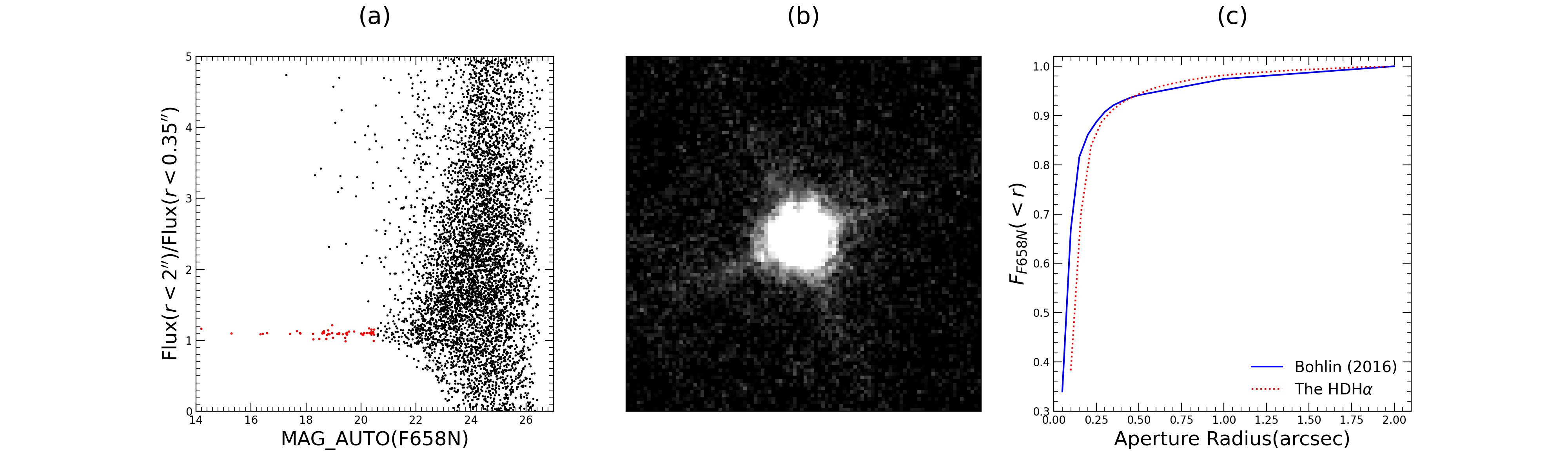
Figure 3: Derivation of the ePSF for the HDH$\alpha$. (a): the flux ratio in different apertures as a function of the narrowband magnitude. The bright and unsaturated stars are marked in red dots; (b): the ePSF in a $\mathbf{\sim 6^{\prime\prime}\times 6^{\prime\prime}}$ box stacked from bright and unsaturated stars in the HDH$\alpha$. The diffraction spike structure of the ePSF is clearly shown here; (c): The light growth curves derived from the ePSF (the red dotted line) and from the latest photometric calibration result of HST (Bohlin, 2016) (the blue solid line).

2.4.2 Astrometry

We check the astrometry between our HDH$\alpha$ image and the HLF images. By matching the sources with S/N $>10$ in both the HDH$\alpha$ catalog and the HLF F606W-band catalog within a radius of $0^{\prime\prime}.1$, we select 1234 sources for the calculations of the astrometric offsets in the two bands. We present the scatter map of astrometric residuals and the distribution of offsets in R.A. and Decl. directions. We fit the distribution to a Gauss function. The mean offset of the astrometric residuals is at the level of $<0^{\prime\prime}.002$, and the 1 $\sigma$ values on R.A. and Decl. are $\mathrm{0^{\prime\prime}.033}$ and $\mathrm{0^{\prime\prime}.032}$, respectively. The offset corresponds to a spatial difference of less than 0.1 pixel (See panel (a) of Fig. 4), which is quite good when considering the positional uncertainties of sources in the HDH$\alpha$. Panel (b) of Fig. 4 shows the astrometric residuals at different positions using the same data as panel (a). To explore the spatial variation of the alignment, we check the residuals at different areas of the HDH$\alpha$, which are composed of different meshes of the HDH$\alpha$ with each mesh’s size of 2000 pixels $\times$ 2000 pixels ($2^{\prime}\times 2^{\prime}$). We present the average value and the direction (vector) of sources in each mesh in panel (b) of Fig. 4. The mean residuals are small across the image, meaning the residual offsets of sources in each mesh are distributed randomly. Therefore, there is no large systematic offset exists.

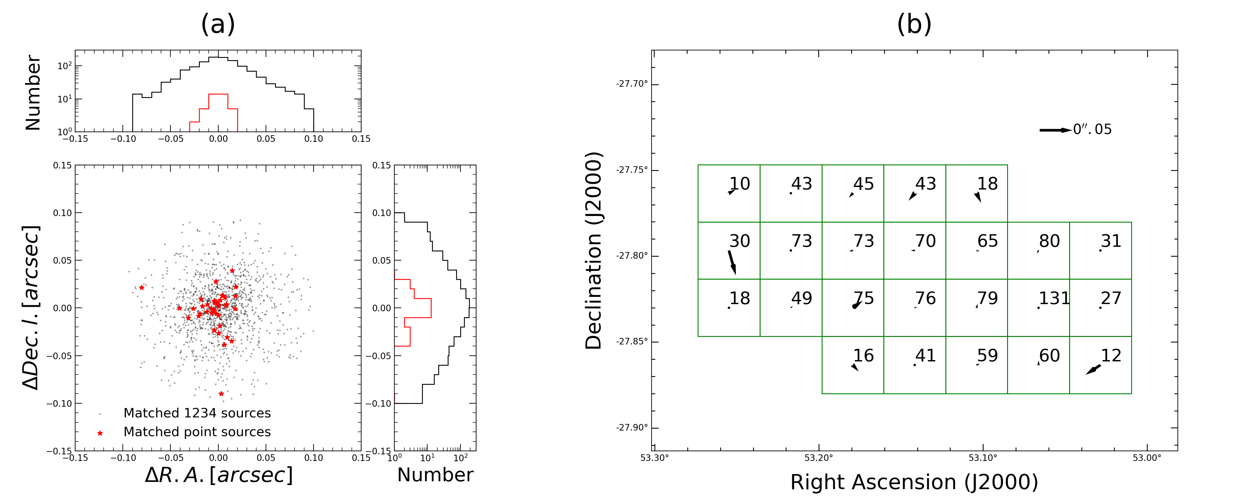
Figure 4: (a): The astrometric residuals calculated from the matched 1234 sources in the HDH$\alpha$ project. The grey and red histograms in the R.A. and Decl. directions show distributions of the residual offsets for all matched sources and a sub-sample of matched point sources, respectively. (b):The spatial distribution of the astrometric residuals of the matched sources. The panel demonstrates the mean residual shown as a vector in each mesh within a size of $2^{\prime}\times 2^{\prime}$, and the number of matched sources used in each mesh in the calculation.

2.4.3 Exposure Time and Depth

We measure the differential and cumulative distributions of the exposure time and the 5$\sigma$ limiting magnitude of the HDH$\alpha$ image. The distributions of exposure time are measured based on the exposure time map generated in Section 2.3.3.

We use the same way as the previous work (e.g. HDUV, Oesch et al., 2018) to estimate the depth of the HDH$\alpha$. We measure the distribution of 5$\sigma$ limiting magnitude by dividing the images into meshes with a size of $\rm 128\ pixels\times 128\ pixels$ ($7^{\prime\prime}.68\times 7^{\prime\prime}.68$). For each mesh, the 5$\sigma$ limiting magnitude is measured by randomly placing empty apertures with a diameter of 0^′′.7 in the background region and estimating the standard deviation of the fluxes in these empty apertures with the zero-point magnitude of 22.75. The zero-point magnitude here is determined with two keywords of PHOTFLAM and PHOTPLAM, which are generated by AstroDrizzle in the image header of the mosaic HDH$\alpha$ image. The results are shown in Fig. 5. In the deepest region, the 5$\sigma$ limiting magnitude of HDH$\alpha$ is 25.8.

Figure 5: The differential (top row) and cumulative (bottom row) distributions of the effective exposure time (left column) and the 5$\sigma$ depth magnitude (right column) in the HDH$\alpha$ project.

We also check the depth of the HDH$\alpha$ by using the same method as Finkelstein et al. (2011), which is summarized as below. Finkelstein et al. (2011) checked the distribution of all detected sources, as well as the statistics of non-detected sources (in empty apertures) in section 23 of GOODS-S (version 2.0, Giavalisco et al., 2004). Three types of limiting magnitudes are defined here, the peak magnitude, the detection limit magnitude, and the 5$\sigma$ depth magnitude. The peak of the magnitude distribution of detected sources defines the peak magnitude. At the 50% peak value in the fainter-end of the distribution, the corresponding magnitude is defined as the detection limit magnitude. The 5$\sigma$ depth magnitude is derived by using the empty aperture method. The distributions of the detected sources in the HDH$\alpha$ are presented in Fig. 6. The statistics of non-detected sources in the HDH$\alpha$ are applied in the same region as that of Finkelstein et al. (2011). We present a comparison of the three kinds of limiting magnitudes from ours and those in Finkelstein et al. (2011) in Tab. 4. All three limiting magnitudes indicate that the HDH$\alpha$ image is about $\sim$0.4$-$0.5 mag deeper than that of Finkelstein et al. (2011).

Figure 6: The magnitude distribution of objects with S/N $\geq$ 5 in the mosaic F658N image of the HDH$\alpha$ project. The peak magnitude is around 25.2 mag here, compared to 24.8 mag in Finkelstein et al. (2011).

Table 4: Depths of the $F658N$ images in the GOODS-S field derived by Finkelstein et al. (2011) and this work.

	Finkelstein+2011	This work
Peak magnitude	24.8 mag	25.2 mag
Detection limit magnitude	25.3 mag	25.8 mag
5$\sigma$ depth magnitude	25.0 mag	25.4 mag
Number of detected sources	3081	3960
Median exposure Time	$\sim$11ks	$\sim$22ks

3 Photometric and spectroscopic data in HDH$\alpha$

3.1 Narrowband Source Detection

Since a few high redshift objects would show extended structures in their emission lines, we use the source detection strategy similar to that of the CANDELS program (Guo et al., 2013; Galametz et al., 2013), which applied the cold mode and the hot mode with SExtractor. The cold mode is designed to detect the bright/extended objects in images without over-deblending, while the hot mode is designed to detect the faint/point objects, especially for objects at high redshift. The parameters of the cold/hot modes used for the HDH$\alpha$ are listed in Tab. 5.

The HDH$\alpha$ narrowband image and the RMS map are used as the detection image and the weight map in SExtractor, respectively. The cold and hot modes are applied to generate corresponding catalogs. There are 7466 and 7520 sources detected in the cold and hot modes, respectively. All objects detected in the cold mode are kept. Objects were detected in the hot mode but not in the Kron aperture. There are 7762 objects in the combined catalog.

Note that the cosmic rays cleaning process of AstroDrizzle in the edge region of the HDH$\alpha$ image might fail because of too few frames covered in these areas. This could bring in the remaining cosmic rays in the combined catalog. We require a minimal effective exposure time cut of 10% of the deepest exposure time to exclude these artifacts. The effective exposure time of each source is defined as the average exposure time of pixels that are enclosed in the photometric aperture. This step successfully filters out fake sources in the edge region. There are 3960 objects in an effective area of 76.1 arcmin².

Table 5: Parameters for the source detection process in the HDH$\alpha$ project.

	Cold Mode	Hot Mode
DETECT_THRESH	1.2	1.0
ANALYSIS_THRESH	5.0	1.0
FILTER	tophat_5.0_5x5	gauss_4.0_7x7
DETECT_MINAREA	5.0	8.0
DEBLEND_NTHRESH	32	64
DEBLEND_MINCONT	0.1	0.001
BACK_SIZE	128	64
BACK_FILTERSIZE	9	5
BACKPHOTO_THICK	100	48

3.2 Multi-band Photometric Data

In order to select emission-line galaxies in the HDH$\alpha$, we use four additional broadband images in the HLF (ACS/WFC F435W, F606W, F775W and F814W). The transmission curves of these filters are shown in Fig. 1.

We run SExtractor in the dual-image mode to measure the aperture fluxes for the HDH$\alpha$ narrowband image and the HLF broadband images, respectively, with the cold-hot strategy described in Section 3.1. We use the HDH$\alpha$ image as the detection image. The aperture photometry is calculated within a circle with a diameter of $0^{\prime\prime}.7$. The aperture correction in each band is applied based on the light growth curve of ePSF we generated in the corresponding band. Then the total flux is calculated as:

$$f_{X,tot}=f_{X,aper}\frac{f_{X}(r_{tot})}{f_{X}(r<r_{aper})}$$ (1)

where X denotes the filter (i.e., F435W, F606W, F775W, F814W or F658N), the $f_{X,aper}$ is the flux encircled in the aperture, and the ratio of $f_{X}(r_{tot})$/$f_{X}(r<r_{aper})$ is measured from the ePSF we generated.

The zero-point magnitude of the HDH$\alpha$ image is described in Section 2.4.3. As for the HLF broadband data, we use the zero-point magnitude provided by the HLF team. We convert the flux after the aperture correction into magnitude using this zero-point. We do not apply any further zero-point correction, which is expected to be very small ($<0.1\rm mag$) according to the previous work (e.g., see Appendix section of Guo et al., 2013; Skelton et al., 2014).

3.3 Broadband-over-narrowband Color Offset

Because the center wavelength of the narrowband filter does not match that of the broadband filter, the corresponding broadband-over-narrowband color of continuum-dominated sources with a non-flat slope would not have a value around zero. We first demonstrate this phenomenon through the calculation. We define the observer-frame equivalent width of an emission line as

$$\mathrm{EW_{obs}}=\Delta\lambda_{NB}\frac{f_{\lambda,NB}-f_{\lambda,BB}}{f_{\lambda,BB}-f_{\lambda,NB}(\Delta\lambda_{NB}/\Delta\lambda_{BB})},$$ (2)

where the $f_{\lambda,NB}$ and $f_{\lambda,BB}$ are the flux densities in the unit of $\mathrm{erg\ cm^{2}\ s^{-1}\ \AA^{-1}}$ of the broadband and the narrowband, respectively. The $\Delta\lambda_{NB}$ and $\Delta\lambda_{BB}$ are the widths (FWHMs) of the corresponding filter, and the center wavelengths of the narrowband filter and the broadband filter are 6584 Å and 5907 Å, respectively. With Eqn. 2, we derive the broadband-over-narrowband color of a continuum-dominated source (EW${}_{\textrm{obs}}$ = 0) as 0.24 mag.

We then use objects with spectroscopic redshifts whose continuum is covered by the F658N narrowband filter to check the broadband-over-narrowband color offset. The redshift information is from Section 4.2 and the emission lines are listed in Tab. 6. Only the bright sources with S/N $\geq$ 10 in narrowband and broadband images are used in this procedure. We adopt the median after the sigma-clipping to remove the impact of the remaining outliers. The sigma-clipped median value and one sigma value of the colors are $\sim 0.27$ mag and $\sigma\sim 0.14$, respectively, which agree with the calculated result above.

To further probe how the broadband color (or the continuum slope) affects the broadband-over-narrowband color offset, we follow Sobral et al. (2013) to investigate the relations between the broadband-over-narrowband color and the broadband color for sources with a bright continuum. The relations between the broadband-over-narrowband color and five different broadband colors are presented in Fig. 7. The median values of the distributions are calculated with the sigma-clipping method. In Fig. 7, we can see that the effect of broadband colors can be ignored when estimating the broadband-over-narrowband color offset.

Figure 7: The relations between the broadband-over-narrowband color and different broadband colors. We investigate the relations using sources with S/N $>$ 10 in the corresponding broadbands as well as only the continuum covered by the F658N narrowband. Most of the sources in our field have relatively red colors, which are reflected by the positive broadband colors and the increasing differences in the central wavelengths of the two corresponding filters.

Table 6: Redshift ranges of line emitters whose emission line could be covered by the F658N narrowband filter.

Emission line	Rest-frame wavelength	Redshift range
Ly$\alpha$	1215.67Å	[4.370, 4.463]
O i	1302.168Å	[4.013, 4.100]
N iv]	1486.496Å	[3.392, 3.468]
C iv	1548.187Å/1550.772Å	[3.210, 3.290]
C III]	1908.734 Å	[2.420, 2.479]
Mg ii]	2795.528Å/2802.705Å	[1.329, 1.376]
[O ii]	3726.032Å/3728.815Å	[0.751, 0.782]
He ii	4685.71Å	[0.393, 0.417]
H$\beta$	4861.333Å	[0.343, 0.366]
[O iii]	4958.911Å/ 5006.843Å	[0.304, 0.339]
H$\alpha$	6562.819Å	[0, 0.012]

Note. — The filter width used to calculate the redshift range is the full width at the 5% maximum (wavelength range: 6528Å-6641Å). The wavelength values of the emission lines are from Kramida et al. (2022).

3.4 Spectroscopic data

The enormous spectroscopic resources in the GOODS-S field help us to validate the redshifts of ELG candidates selected in the HDH$\alpha$. To obtain the spectroscopic redshifts for sources identified with HDH$\alpha$, the following public spectroscopic catalogs are used, including (1)The compilation of the spectroscopic catalog of VLT, which assembles the major results of large spectroscopic surveys between 2001-2012 (Vanzella et al., 2008; Le Fèvre et al., 2005; Szokoly et al., 2004; Croom et al., 2001; Dickinson et al., 2004; van der Wel et al., 2004; Bunker et al., 2003; Stanway et al., 2004; Doherty et al., 2005; Cristiani et al., 2000; Strolger et al., 2004; Stanway et al., 2004; Popesso et al., 2009; Balestra et al., 2010; Mignoli et al., 2005; Ravikumar et al., 2007; Silverman et al., 2010; Kurk et al., 2013); (2)The VANDELS DR4 catalog based on VANDELS spectroscopic survey (Garilli et al., 2021); (3)The MUSE-Wide catalog (Urrutia et al., 2019); (4) The catalog of the MUSE-HUDF survey (Bacon et al., 2022).

Table 7: Summary of spectroscopic catalogs in the GOODS-S region used in this work.

	Total	Number	Number
Catalog name		of sources	of matched
	Number	in HDH$\alpha$	with HDH$\alpha$
The compilation catalog1	7146	2115	1095
VANDELS DR4 catalog2	1017	252	97
MUSE-Wide catalog3	1602	1422	709
MUSE-HUDF catalog4	2221	2221	426

We also note that there are grism catalogs of HST based on the PEARS program (PI: Sangeeta Malhotra, Program ID: 10530, Pirzkal et al., 2013) and the 3D-HST program(PI: Pieter van Dokkum, Program ID: 12177, 12328, Brammer et al., 2012; Momcheva et al., 2016). There are no HDH$\alpha$ ELG or LAE candidates matched with sources in the PEARS catalog. For the 3D-HST catalog, we found that 37 sources in HDH$\alpha$ confirmed at $z=0$ from ground-based spectroscopic surveys show $z>0.1$ in the 3D-HST grism catalog. Therefore, we do not use these two catalogs in this work.

We plot the coverage of the MUSE-Wide, the MUSE-HUDF, the PEARS, and the 3D-HST, along with several imaging data sets in the GOODS-S filed in Fig 2. The total number of sources in various catalogs and in the HDH$\alpha$ coverage are listed in Tab. 7. We perform a cross matching between the redshift catalogs described above and the HDH$\alpha$ catalog with a matching radius of $\boldmath 0^{\prime\prime}.6\unboldmath$. There are 1,799 sources that have at least one detection in these spectroscopic catalogs. For those sources with more than one redshifts in the spectroscopic catalogs, their redshifts are chosen based on the spectral resolution and quality of the corresponding catalogs.

4 Emission-line Galaxies in HDH$\alpha$

In this section, we describe our selection procedure for ELGs with the HDH$\alpha$ data. The selection criteria of ELGs are discussed in Section 4.1. We discuss the confirmed ELGs in Section 4.2. Finally, the depths of emission lines are discussed in Section 4.3.

4.1 ELGs’ selection criteria

HDH$\alpha$ ELGs should have a strong emission line covered by the F658N narrowband filter, thus can be selected by their broadband-over-narrowband color excess (F606W-F658N) to ensure the existence of a strong emission line, such as H$\alpha$ at $z\sim$0.0, [O iii] at $z\sim$ 0.3, [O ii] at $z\sim$ 0.8, or Ly$\alpha$ at $z\sim$ 4.4 (see Tab. 6 for details). Besides the color excess, we also require a line significance parameter on the color excess defined as $\Sigma=\frac{BB-NB}{\sqrt{\Delta BB^{2}+\Delta NB^{2}}}$, where BB and NB represent the magnitudes in broadband and narrowband, and $\Delta BB$ and $\Delta NB$ are the errors of magnitude in broadband and narrowband, respectively.

Since all HDH$\alpha$ sources are covered by the F435W band, according to the Lyman-break technique the detections and non-detections of F435W would divide the redshifts of HDH$\alpha$ sources at $z<4$ and $z\gtrsim 4$, respectively. For the latter case, ELGs at $z\gtrsim 4$ selected with HDH$\alpha$ would be LAEs at $z\sim$ 4.4. We discuss the two samples separately below.

Figure 8: (a): The color and the line significance ($\Sigma$) diagram for the continuum sources (grey dots), 156 ELG candidates (squares), and 53 LAE candidates (triangles) in HDH$\alpha$. The continuum sources refer to those not selected as neither ELG candidates at $z<4$ nor LAE candidates at $z\sim 4.4$. The dashed line and dotted line represent the color and line significance cuts used for the selections of ELG candidates at $z<4$ and LAE candidates at $z\sim$ 4.4, respectively (see Section 4.1.1 and Section 4.1.2). (b): The color-magnitude diagram of the continuum sources, ELG candidates at $z<4$, and LAE candidates at $z\sim 4.4$ in HDH$\alpha$. The symbols are the same as in panel (a). Colors of F606W-F658N $>6$ are set to $=6$ for display only. The two horizontal lines mark the color cuts used in the selection criteria for ELGs at $z<4$ and LAEs at $z\sim 4.4$, which correspond to a rest frame EW ${\sim 30}$ Å at $z\sim 0.77$ and ${\sim 25}$ Å at $z\sim 4.4$, respectively.

4.1.1 ELG candidates at $z<4$

We select the ELG candidates at $z<4$ using the selection criteria below, which include an S/N cut on the narrow-band detection, a color cut corresponding to the equivalent-width cut of an emission line, and a significance of the color excess. These criteria are similar to those of the ground-based ELG surveys (e.g., Sobral et al., 2015; Khostovan et al., 2015, 2020). To further exclude cosmic rays or artifacts, as well as ensure the redshifts at $z<4$, we require sources with reliable signals in the bluer broadband image (here the F435W image). The following selection criteria are applied to select ELG candidates at $z<4$:

$$S/N_{\rm F658N} > 5.0,$$ (3)

$$F606W-F658N > 0.72,$$

$$\Sigma=\frac{F606W-F658N}{\sqrt{\Delta{F606W}^{2}+\Delta{F658N}^{2}}} > 5.0,$$

$$S/N_{\rm F435W} > 5.0,$$

where the $S/N_{\rm F658N}$ and the $S/N_{\rm F435W}$ are the signal-to-noise ratio of objects in the F658N image and the F435W image, respectively. The color cut is set to 0.72, which corresponds to observer-frame equivalent widths of 52.5 Å, which is the same as the previous survey (Khostovan et al., 2020). This color cut corresponds to rest-frame equivalent widths of 52.5 Å at $z\sim 0.0$, 39.8 Å at $z\sim 0.32$, and 30.0 Å at $z\sim 0.77$. The significance of the color excess $\Sigma$ is often set to 3 according to previous studies (e.g., Sobral et al., 2015; Khostovan et al., 2015, 2020). Here we set this to a value of 5 to exclude more contamination indicated by the spectroscopic data (see Sec. 4.2.1 for details).

There are 212 ELG candidates at $z<4$ selected with the above criteria. After the visual inspection, 4 objects are excluded because of the cosmic rays or artifacts. The remaining 208 ELG candidates should include H$\alpha$ emitters at $z\sim$0.0, [O iii] emitters at $z\sim$ 0.3, [O ii] emitters at $z\sim$ 0.8, and other contamination. Note that Galactic stars could be included in the sample of H$\alpha$ emitters.

To exclude stars in the sample of ELG candidates, especially in the H$\alpha$ emitters, we utilize the star selection method of Dahlen2010, which is based on the F435W-J color and J-IRAC1 color. We select 52 objects using this method. 27 of the 52 objects have available redshifts, and all these 27 objects are identified as stars according to their spectra. Furthermore, these 27 stars are all the HDH$\alpha$ ELG candidates with available redshifts at $z\sim$ 0. Therefore, we exclude all the 52 objects from the ELG candidates at $z<4$ (see the Appendix section for details).

Finally, we select 156 objects as ELG candidates at $z<4$ in HDH$\alpha$. The sample should include strong ELGs, such as [Oiii] emitters at $z\sim$ 0.32 and [Oii] emitters at $z\sim$ 0.77. All these ELG candidates at $z<4$ are marked with squares in the color-line significance($\Sigma$) diagram and the color-magnitude diagram (see panels (a) and (b) of Fig. 8).

4.1.2 LAE candidates at $z\sim 4.4$

The selection criteria for LAEs at $z\sim$ 4.4 are summarized as below, including an S/N cut on the narrow-band detection, a color cut corresponding to the equivalent-width cut of the Ly$\alpha$ line, a line significance parameter of the color excess, and a blue band (F435W here) non-detection. These criteria are similar to those of the ground-based LAE surveys (e.g., Rhoads et al., 2000; Finkelstein et al., 2008). We require a red band (F775W or F814W) detection to further exclude cosmic ray events and other artifacts.

The following selection criteria are applied to select LAE candidates:

$$S/N_{\rm F658N\ Auto}>5.0\quad\|\quad S/N_{\rm F658N\ Aper} > 5.0,$$ (4)

$$F606W-F658N > 1.2,$$

$$\Sigma=\frac{F606W-F658N}{\sqrt{\Delta{F606W}^{2}+\Delta{F658N}^{2}}} > 3.0,$$

$$S/N_{\rm F435W} < 3.0,$$

$$S/N_{\rm F775W}>3.5\quad\|\quad S/N_{\rm F814W} > 3.5,$$

where the $S/N_{\rm F658N\ Aper}$ and $S/N_{\rm F658N\ Auto}$ are the signal-to-noise ratios in the F658N band within an aperture of diameter $0^{\prime\prime}.7$ and a Kron aperture, respectively. The $S/N_{\rm F775W}$ and $S/N_{\rm F814W}$ are the signal-to-noise ratios of objects in F775W and F814W bands within an aperture of diameter $0^{\prime\prime}.7$, respectively. The $S/N_{\rm F435W}$ is measured using an aperture of diameter $0^{\prime\prime}.5$ to avoid the contamination from nearby objects. The color threshold is set to 1.2, corresponding to rest-frame equivalent width of $\sim 25$ Å  at $z=4.4$. We require that the LAEs cannot be detected in the F435W band because LAEs at $z=4.4$ should be drop-outs at the F435W band due to their Lyman break. We also require the sources to be detected in the F775W or F814W band to exclude false detections.

We selected 66 LAE candidates with the above criteria. After the visual inspection, there are 53 LAE candidates left, which are marked as triangles in the color-line significance($\Sigma$) diagram and the color-magnitude diagram (see panels (a) and (b) of Fig. 8).

4.2 Spectroscopic confirmation of HDH$\alpha$ ELGs

In this section, we discuss the selected ELG candidates with available spectroscopic redshifts, including [O iii] emitters at $z\sim$ 0.3, [O ii] emitters at $z\sim$ 0.8, and LAEs at $z\sim 4.4$. In Fig. 9, we present the redshift distribution and the color-redshift diagram for all sources with spectroscopic redshifts, ELG candidates at $z<4$, and LAE candidates. As we introduced in Section 1, the narrowband excess method is only sensitive to galaxies at specific redshifts, where their emission lines are redshifted to the bandpass of the F658N filter. Here we give the expected redshift ranges of 9 emission line emitters in Tab. 6. These emitters’ redshift ranges are marked as grey regions in Fig. 9.

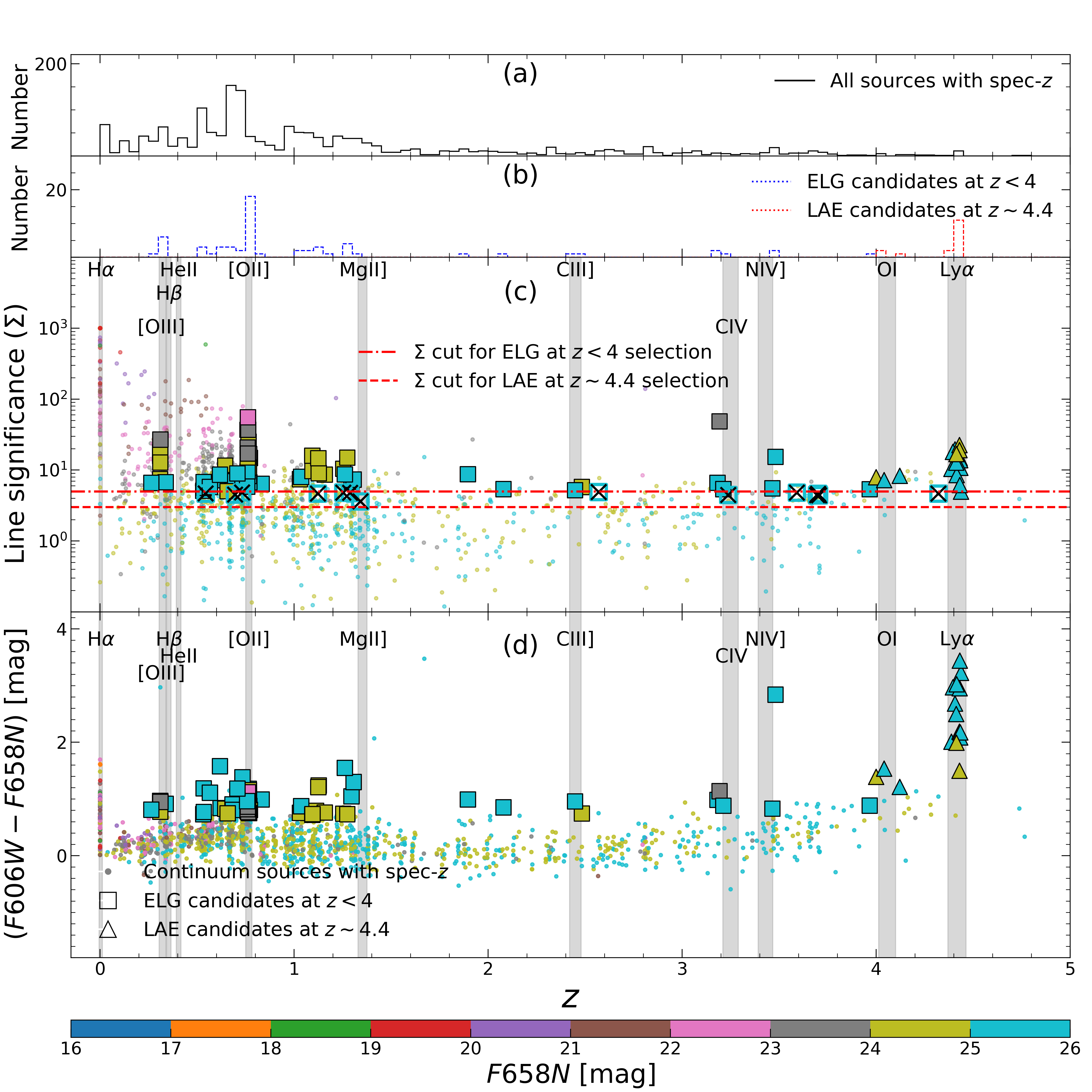
Figure 9: (a): The redshift distribution of all HDH$\alpha$ sources with available redshifts. (b): The redshift distributions of ELG candidates at $z<4$ and LAE candidates $z\sim 4.4$ with available redshifts in the HDH$\alpha$, which are marked by the blue dashed and the red dashed histograms, respectively. (c): The line significance ($\Sigma$) of the color excess and redshift diagram of continuum sources, ELG candidates at $z<4$, and LAE candidates $z\sim 4.4$ in the HDH$\alpha$. The grey vertical regions mark the redshift ranges of the corresponding emission lines. The symbols of ELG candidates at $z<4$ and LAE candidates at $z\sim 4.4$ are similar to those in Fig. 8. The open squares with cross marks represent sources with F658N-F606W color $>$ 0.72 but line significance $\Sigma<5$, which are not valid ELGs based on their redshifts. The symbols’ color is encoded with their narrowband magnitudes shown in the bottom color bar. We can see that fainter sources tend to have smaller significance values of their color excesses. (d): The color-redshift diagram of continuum sources, ELG candidates at $z<4$, and LAE candidates at $z\sim 4.4$ with available redshifts. The symbols are similar to those in panel (c). In this panel, sources fainter than 26 mag in F658N are excluded.

4.2.1 Confirmed ELGs at $z<4$

Among the 156 ELG candidates at $z<4$ selected with HDH$\alpha$, 61 are matched with the spectroscopic catalogs introduced in Section 3.4. We classify these ELG candidates further by matching the redshifts ranges of the corresponding lines in Tab. 6 and by inspecting their spectra. In the following paragraphs, we separate the sample into sub-samples at $z<1$ and at $1\lesssim z<4$ for clear discussions.

We have cross-matched 38 ELG candidates with spectroscopic redshifts at $z<1$. Based on their redshifts, we classify 6 objects as [O iii] emitters and 18 objects as [O ii] emitters. Through visual inspection of their spectra, we find that all 6 [O iii] emitters and 16 out of the 18 [O ii] emitters show the corresponding emission lines within the wavelength range captured by the F658N filter. The remaining two [O ii] emitters are confirmed by the relatively shallow MUSE-WIDE survey, which have their strong [O iii] lines. For the other 14 sources at $z<1$, we analyze both their spectra and their broadband and narrowband images. Our analysis reveals no significant emission lines within the F658N filter’s wavelength range in their spectra. Further examination of their broadband and narrowband images shows that the majority of these sources (10/14) appear compact in narrowband but extended in broadband. Since the narrowband image serves as the detection image (see Section 3.2), this discrepancy results in an underestimation of broadband flux, leading to an overestimation of the broadband-over-narrowband color, thereby erroneously categorizing them as ELG candidates. The remaining 4 objects appear compact in both broadband and narrowband images. Given their redshifts, the Balmer decrement and the 4000 Å break contribute to a reduced flux in F606W, enhancing the broadband-over-narrowband color and consequently, misidentifying these objects as ELG candidates.

We have cross-matched 23 ELG candidates with spectroscopic redshifts in the range of $1\lesssim z<4$. Upon inspecting their spectra, we identify emission lines within the wavelength range of the F658N filter in 4 objects. These include 3 Mg ii] emitter at $z\sim 1.3$ and one C iii] emitter at $z\sim 2.4$. Additionally, we also confirm one C iv emitter at $z\sim 3.19$ based on the broad line partially covered by the F658N filter. This object is matched with a QSO, CXOCDFS J033242.8-274702 from Luo et al. (2017). For the other 18 candidates, we thoroughly examine their spectra, broadband, and narrowband images. 5 of these candidates at $z\sim 1$ show a red continuum, inadvertently enhancing their broadband-over-narrowband colors and leading to their inaccurate selection as ELG candidates. Among the remaining 13, we find no continuum in their spectra. A closer look at their images reveals 8 of them to be compact in narrowband yet extended in broadband, which would overestimate the broadband-over-narrowband color, causing them to be mistakenly identified as ELG candidates. The final 5 objects, compact in both imaging modes, likely have large F606W-F658N colors due to continuum features that their spectra are too shallow to reveal.

It is also noticeable that faint ELG candidates from HDH$\alpha$, especially for those fainter than 25 mag in F658N, would contaminate the selection of the ELG candidates. For example, when improving the significance cut of the color excesses in the ELG selection from 3 to 5, we exclude 14 ELG candidates with redshifts, which are all contamination and fainter than 25 mag in the F658N band (see panel (c) of Fig. 9).

In summary, of all the ELG candidates at $z<$ 4, there are 6 and 18 galaxies confirmed as [O iii] emitters at $z\sim$ 0.32 and [O ii] emitters at $z\sim$ 0.77, respectively. Their positions and photometric data are presented in Tab. 8. We also present these sources’ narrowband and broadband thumbnail images and 1-d spectra in Fig. 10 and Fig 11.

Table 8: The catalog of [O iii] and [O ii] emission line galaxies with spectroscopic confirmation in the HDH$\alpha$ project.

ID	R.A.	Dec.	F435W	F606W	F658N	F775W	F814W	$z$	Reference	Line flux	Type
	(Degree)	(Degree)	(ABmag)	(ABmag)	(ABmag)	(ABmag)	(ABmag)			($10^{-17}\mathrm{erg\ cm^{2}\ s^{-1}}$   )
$282^{*}$	53.114915	-27.765746	$25.93\pm 0.03$	$25.29\pm 0.02$	$24.43\pm 0.12$	$25.20\pm 0.03$	$25.07\pm 0.01$	$0.309$	U19	$1.70^{+0.47}_{-0.42}$	[O iii]
353	53.152608	-27.769387	$26.93\pm 0.02$	$25.97\pm 0.00$	$25.06\pm 0.14$	$25.63\pm 0.00$	$25.53\pm 0.02$	$0.338$	M05	$1.00^{+0.29}_{-0.26}$	[O iii]
2076	53.096750	-27.819529	$25.97\pm 0.05$	$25.34\pm 0.01$	$24.41\pm 0.06$	$25.22\pm 0.03$	$25.22\pm 0.01$	$0.310$	U19	$1.82^{+0.24}_{-0.23}$	[O iii]
2082	53.093190	-27.819698	$26.05\pm 0.05$	$25.33\pm 0.01$	$24.37\pm 0.05$	$25.17\pm 0.03$	$25.13\pm 0.01$	$0.310$	U19	$1.98^{+0.23}_{-0.22}$	[O iii]
3404	53.083948	-27.858922	$25.83\pm 0.06$	$24.98\pm 0.01$	$24.20\pm 0.06$	$24.82\pm 0.03$	$24.70\pm 0.01$	$0.310$	U19	$1.86^{+0.30}_{-0.28}$	[O iii]
3445	53.084732	-27.861410	$25.33\pm 0.04$	$24.57\pm 0.01$	$23.63\pm 0.03$	$24.45\pm 0.02$	$24.33\pm 0.00$	$0.311$	U19	$3.86^{+0.29}_{-0.28}$	[O iii]
215	53.167378	-27.762830	$26.84\pm 0.02$	$26.51\pm 0.01$	$25.33\pm 0.16$	$26.04\pm 0.01$	$25.87\pm 0.03$	$0.767$	B22	$0.97^{+0.27}_{-0.24}$	[O ii]
669	53.170724	-27.782031	$26.38\pm 0.01$	$25.30\pm 0.00$	$24.31\pm 0.06$	$24.28\pm 0.00$	$24.12\pm 0.01$	$0.767$	B22	$2.15^{+0.25}_{-0.23}$	[O ii]
700	53.152808	-27.782777	$25.53\pm 0.01$	$25.27\pm 0.00$	$24.18\pm 0.04$	$24.89\pm 0.00$	$24.68\pm 0.01$	$0.765$	V08	$2.63^{+0.20}_{-0.19}$	[O ii]
1034	53.107234	-27.792313	$26.33\pm 0.07$	$26.02\pm 0.03$	$25.14\pm 0.13$	$25.54\pm 0.05$	$25.37\pm 0.02$	$0.769$	U19	$0.89^{+0.28}_{-0.25}$	[O ii]
1157	53.097031	-27.795813	$25.71\pm 0.04$	$25.12\pm 0.01$	$24.27\pm 0.05$	$24.38\pm 0.01$	$24.26\pm 0.01$	$0.764$	V08	$1.91^{+0.23}_{-0.22}$	[O ii]
1572	53.113281	-27.807036	$25.43\pm 0.03$	$25.13\pm 0.01$	$24.32\pm 0.05$	$24.52\pm 0.02$	$24.41\pm 0.01$	$0.772$	U19	$1.74^{+0.24}_{-0.23}$	[O ii]
2502	53.030231	-27.829806	$24.07\pm 0.00$	$23.71\pm 0.00$	$22.92\pm 0.02$	$23.16\pm 0.00$	$23.08\pm 0.00$	$0.760$	LF05	$6.11^{+0.33}_{-0.32}$	[O ii]
2779	53.073088	-27.837126	$25.30\pm 0.04$	$25.08\pm 0.01$	$24.27\pm 0.05$	$24.42\pm 0.02$	$24.35\pm 0.00$	$0.763$	U19	$1.82^{+0.22}_{-0.21}$	[O ii]
2848	53.177903	-27.839265	$25.44\pm 0.02$	$24.53\pm 0.01$	$23.78\pm 0.04$	$23.58\pm 0.01$	$23.47\pm 0.00$	$0.768$	R07	$2.63^{+0.32}_{-0.31}$	[O ii]
3034	53.168674	-27.844082	$26.40\pm 0.06$	$26.08\pm 0.03$	$25.01\pm 0.13$	$25.47\pm 0.04$	$25.29\pm 0.01$	$0.767$	U19	$1.20^{+0.30}_{-0.27}$	[O ii]
3085	53.163797	-27.845878	$26.26\pm 0.05$	$26.05\pm 0.03$	$24.90\pm 0.10$	$25.42\pm 0.04$	$25.24\pm 0.01$	$0.767$	U19	$1.42^{+0.27}_{-0.25}$	[O ii]
3132	53.091967	-27.847772	$26.63\pm 0.09$	$26.11\pm 0.03$	$25.02\pm 0.11$	$25.49\pm 0.04$	$25.28\pm 0.01$	$0.760$	U19	$1.21^{+0.27}_{-0.24}$	[O ii]
3207	53.087621	-27.850664	$25.82\pm 0.04$	$25.58\pm 0.02$	$24.52\pm 0.07$	$25.21\pm 0.04$	$25.07\pm 0.01$	$0.761$	U19	$1.89^{+0.26}_{-0.24}$	[O ii]
3242	53.088701	-27.851943	$24.51\pm 0.01$	$23.93\pm 0.00$	$23.16\pm 0.02$	$23.24\pm 0.01$	$23.13\pm 0.00$	$0.764$	P09;B10	$4.78^{+0.26}_{-0.26}$	[O ii]
3439	53.126783	-27.861306	$25.02\pm 0.02$	$24.19\pm 0.00$	$23.37\pm 0.04$	$23.22\pm 0.01$	$23.09\pm 0.00$	$0.761$	P09;B10	$4.23^{+0.40}_{-0.39}$	[O ii]
3506	53.113364	-27.864067	$24.25\pm 0.01$	$24.04\pm 0.00$	$22.92\pm 0.02$	$23.77\pm 0.01$	$23.59\pm 0.00$	$0.762$	U19	$8.53^{+0.31}_{-0.30}$	[O ii]
3526	53.076115	-27.865446	$25.09\pm 0.01$	$24.73\pm 0.01$	$23.86\pm 0.05$	$24.18\pm 0.01$	$24.07\pm 0.00$	$0.762$	U19	$2.85^{+0.33}_{-0.32}$	[O ii]
3531	53.087015	-27.865916	$26.53\pm 0.04$	$26.11\pm 0.03$	$25.15\pm 0.16$	$25.46\pm 0.05$	$25.40\pm 0.01$	$0.758$	U19	$0.96^{+0.35}_{-0.30}$	[O ii]

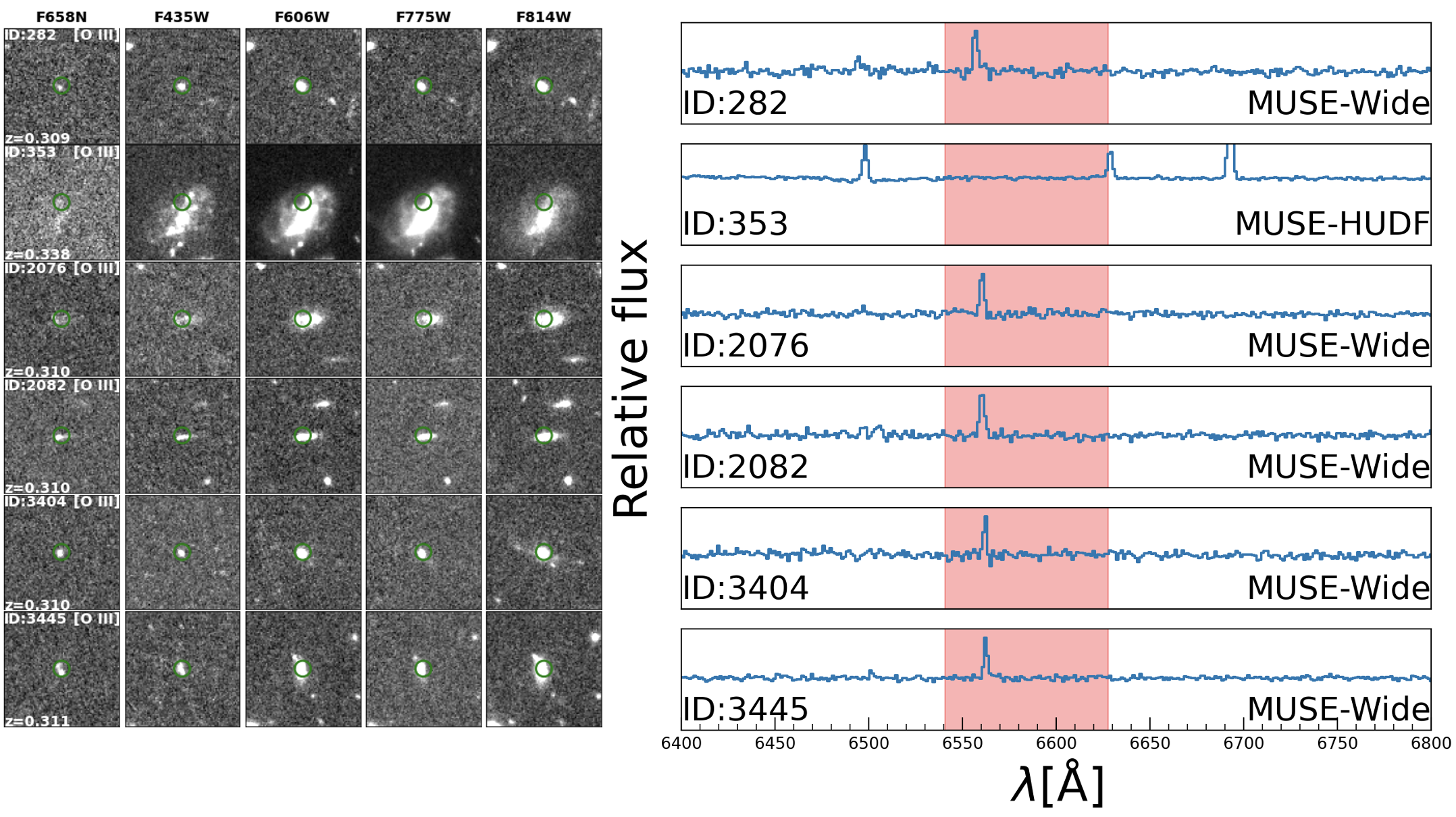
Figure 10: Left panel: The narrowband and broadband thumbnail images of [O iii] emitters at $z\sim$ 0.3. Each thumbnail image has a size of $~{}\sim 5^{\prime\prime}\times 5^{\prime\prime}$, and a green circle with a diameter of $0^{\prime\prime}.7$ in the center. The band information (from left to right: F658N, F435W, F606W, F775W, F814W) of each column is labeled at the top. The emission line type, the catalog ID, and the redshift value are labeled in the first column for each source. Right panel: The 1D spectra of [O iii] emitters at $z\sim 0.3$. The shaded regions demonstrate the coverage of the F658N filter. The facilities used to obtain the spectra are marked.

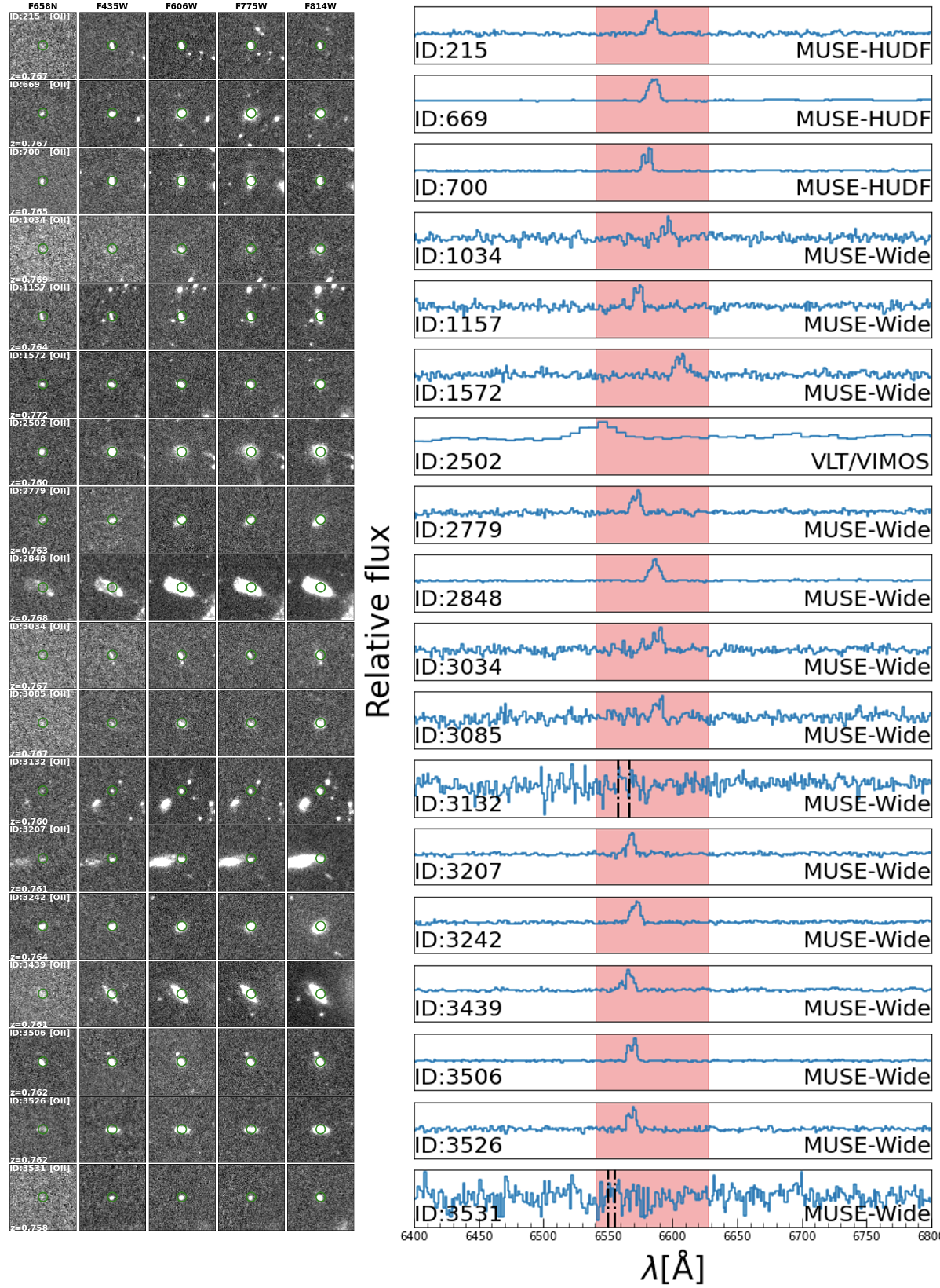
Figure 11: Same as Fig. 10 but for [O ii] emitters at $z\sim$ 0.75-0.77. 2 out of 18 objects (ID: 3132, ID: 3531) do not show [O ii] lines in their spectra but are confirmed by their [O iii] lines. Their [O ii] lines in the wavelength locations are marked by the dashed black lines.

4.2.2 Confirmed LAEs at $z\simeq 4.4$

There are 16 out of 53 LAE candidates ($30\%$) matched with the spectroscopic catalogs introduced in Section 3.4. Among those 16 sources, 13 LAE candidates are finally confirmed as LAEs at $z\sim 4.4$ with the ground-based spectroscopic surveys (see Tab. 9). Note that one LAE confirmed by the MUSE-HUDF survey is classified as an [O iii] emitter by the MUSE-Wide survey mistakenly. There are also three sources at $z\simeq 4.0$ selected as LAE candidates. From their spectra, these three sources may have weak [O i] lines covered by the F658N filter. We therefore exclude these 3 candidates as true LAEs. The final success rate of the LAE candidates’ confirmation is 81.25%, which is slightly higher than the typical value of $\sim 70\%$ (e.g., Zheng et al., 2013; Hu et al., 2017; Harish et al., 2022) in previous works based on the ground-based telescope.

Compared to the sample of ELG at $z<4$ candidates, the sample of LAE candidates has a lower fraction in the spectroscopic coverage but a higher fraction in the spectroscopic confirmation. The low fraction of the spectroscopic coverage is caused by the relatively faint continuum of these LAE candidates. Most of such sources have narrowband magnitudes in the range of 25$-$26, and their colors are very large (see Fig. 13). Thus, the continuum of these sources is often faint, which prevents the spectroscopic follow-up surveys that often target bright broadband sources.

Finally, there are 13 LAE candidates confirmed as LAEs at $z\sim 4.4$. These sources’ positions and photometric data are presented in Tab. 9. The narrowband and broadband thumbnail images and 1-d spectra of LAEs are shown in Fig. 12.

Table 9: The catalog of Ly$\alpha$ emitters with spectroscopic confirmation in the HDH$\alpha$ project.

ID	R.A.	Dec.	F435W	F606W	F658N	F775W	F814W	$z$	Reference	Line flux	Type
	(Degree)	(Degree)	(ABmag)	(ABmag)	(ABmag)	(ABmag)	(ABmag)			($10^{-17}\mathrm{erg\ cm^{2}\ s^{-1}}$   )
657	53.181079	-27.781187	$-99.00^{*}$	$28.09\pm 0.03$	$25.41\pm 0.14$	$27.30\pm 0.02$	$27.03\pm 0.09$	$4.411$	B22	$1.39^{+0.21}_{-0.19}$	Ly$\alpha$
854	53.192930	-27.786922	$-99.00^{*}$	$27.86\pm 0.02$	$25.85\pm 0.19$	$26.95\pm 0.01$	$27.07\pm 0.09$	$4.393$	B22	$0.84^{+0.21}_{-0.17}$	Ly$\alpha$
878	53.137240	-27.787397	$34.11\pm 15.91$	$28.57\pm 0.04$	$25.60\pm 0.16$	$28.76\pm 0.07$	$29.29\pm 0.56$	$4.399$	B22	$1.20^{+0.21}_{-0.18}$	Ly$\alpha$
928	53.114967	-27.789050	$28.80\pm 0.70$	$28.91\pm 0.62$	$25.68\pm 0.20$	$27.93\pm 0.41$	$28.52\pm 0.31$	$4.438$	U19	$1.13^{+0.28}_{-0.26}$	Ly$\alpha$
1540	53.175746	-27.806146	$-99.00^{*}$	$28.84\pm 0.05$	$25.89\pm 0.19$	$28.20\pm 0.04$	$27.94\pm 0.18$	$4.434$	B22	$0.92^{+0.20}_{-0.17}$	Ly$\alpha$
1687	53.110863	-27.809801	$28.04\pm 0.33$	$27.29\pm 0.10$	$25.20\pm 0.11$	$26.97\pm 0.16$	$27.06\pm 0.08$	$4.433$	U19	$1.54^{+0.24}_{-0.22}$	Ly$\alpha$
$2005^{\dagger}$	53.204212	-27.817288	$29.44\pm 0.67$	$26.95\pm 0.06$	$24.76\pm 0.08$	$26.45\pm 0.10$	$26.25\pm 0.04$	$4.429$	F11;G21	$2.36^{+0.23}_{-0.22}$	Ly$\alpha$
2233	53.128212	-27.823525	$-99.00^{*}$	$27.45\pm 0.17$	$25.28\pm 0.11$	$26.64\pm 0.12$	$26.65\pm 0.05$	$4.434$	U19	$1.46^{+0.22}_{-0.21}$	Ly$\alpha$
2579	53.175339	-27.831462	$30.00\pm 1.53$	$28.58\pm 0.29$	$25.56\pm 0.21$	$28.18\pm 0.53$	$28.17\pm 0.26$	$4.415$	U19	$1.25^{+0.31}_{-0.27}$	Ly$\alpha$
$2659^{\dagger}$	53.225164	-27.833627	$-99.00^{*}$	$25.78\pm 0.01$	$24.28\pm 0.08$	$24.87\pm 0.01$	$24.84\pm 0.00$	$4.430$	F11;P09;B10	$3.02^{+0.34}_{-0.32}$	Ly$\alpha$
2874	53.162809	-27.839717	$28.78\pm 0.50$	$27.87\pm 0.14$	$25.37\pm 0.14$	$27.23\pm 0.22$	$27.49\pm 0.10$	$4.413$	U19	$1.42^{+0.24}_{-0.22}$	Ly$\alpha$
3049	53.159479	-27.844401	$29.10\pm 0.68$	$29.27\pm 0.52$	$25.83\pm 0.22$	$27.83\pm 0.38$	$28.65\pm 0.23$	$4.431$	U19	$1.00^{+0.26}_{-0.23}$	Ly$\alpha$
$3296^{\dagger}$	53.165752	-27.854247	$29.49\pm 0.97$	$26.36\pm 0.03$	$24.37\pm 0.11$	$25.54\pm 0.05$	$25.42\pm 0.01$	$4.414$	F11	$3.25^{+0.47}_{-0.43}$	Ly$\alpha$

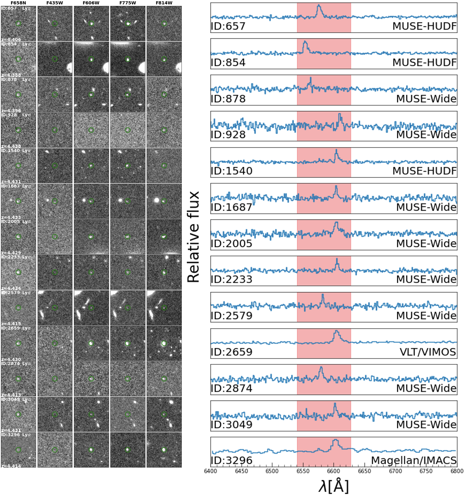
Figure 12: Same as Fig. 10 but for Ly$\alpha$ emitters at $z\sim$ 4.4.

4.3 Depths of Emission Lines in HDH$\alpha$

Here we calculate the depths of emission lines of ELGs candidate in the HDH$\alpha$. The emission line fluxes $f_{line}$ of HDH$\alpha$ sources are defined as:

$${f_{line}=\Delta\lambda_{NB}\left(\frac{f_{\lambda,NB}-f_{\lambda,BB}}{1-\frac{\Delta\lambda_{NB}}{\Delta\lambda_{BB}}}\right)},$$ (5)

where the $f_{\lambda,BB}$ and $f_{\lambda,NB}$ are the flux densities in the unit of $\mathrm{erg\ cm^{2}\ s^{-1}\ \AA^{-1}}$ of the F606W band and the F658N band, and the $\Delta\lambda_{BB}$ and $\Delta\lambda_{NB}$ are the filter widths of the broadband and narrowband, respectively. We present the relation between the line fluxes and the colors of all sources, ELG candidates at $z<4$, and LAE candidates at $z\sim 4.4$ in Fig. 13. The redshifts of sources matched successfully with spectroscopic catalogs are encoded by the color bar. We also plot the different limiting magnitudes in the F658N band in Fig. 13, which shows that the minimum line fluxes of the candidates depend on both the color cut and the limiting F658N magnitude we used in selecting ELGs at $z<4$ or LAEs $z\sim 4.4$. With a smaller color cut and deeper F658N data, a fainter line flux can be probed. We define the depths of our ELG candidates at $z<4$ (LAE candidates at $z\sim 4.4$) as the minimum line fluxes when the color cut is set to 0.72 (1.2) and the limiting F658N magnitude is set to 25.8. Then the depths of emission lines in the HDH$\alpha$ project are $3.9\times 10^{-18}\mathrm{erg\ cm^{2}\ s^{-1}}$ and $6.4\times 10^{-18}\mathrm{erg\ cm^{2}\ s^{-1}}$ for ELG candidates at $z<4$ and LAE candidates at $z\sim 4.4$, respectively. For those confirmed ELGs (LAEs), the minimum and median line fluxes are $8.9\times 10^{-18}\mathrm{erg\ cm^{2}\ s^{-1}}$ and $1.9\times 10^{-17}\mathrm{erg\ cm^{2}\ s^{-1}}$ ($8.4\times 10^{-18}\mathrm{erg\ cm^{2}\ s^{-1}}$ and $1.4\times 10^{-17}\mathrm{erg\ cm^{2}\ s^{-1}}$), respectively.

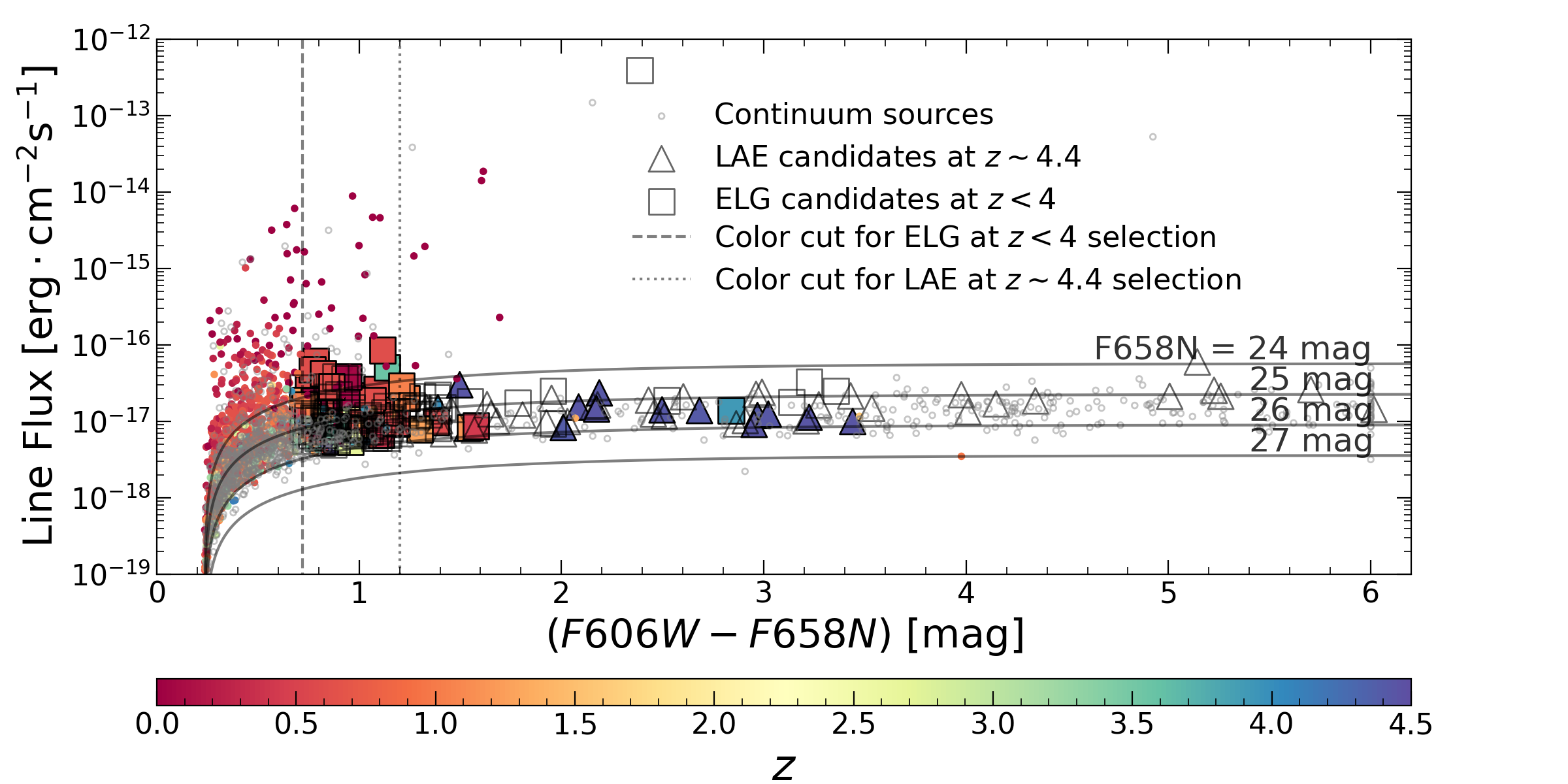
Figure 13: The line flux and F606W-F658N color diagram of the continuum-dominated sources, ELG candidates at $z<4$, and LAE candidates at $\sim 4.4$ in the HDH$\alpha$. The symbols are similar to those in Fig. 8. The open symbols and color-filled symbols represent sources without and with spectroscopic redshifts, respectively. Their redshifts are encoded by the color bar at the bottom. The solid lines are the curves of NB magnitude that step from 24 to 27 mag. The vertical dotted and dashed lines indicate the color cut values for ELGs at $z<4$ and LAEs at $z\sim$4.4, respectively.

5 SUMMARY

We present the Hubble Deep Hydrogen Alpha (HDH$\alpha$) project, which introduces the deepest narrowband imaging data with HST. The HDH$\alpha$ field covers a partial area of the GOODS-S field with the HST/ACS F658N imaging. This paper is the first HDH$\alpha$ paper in a series.

We have reduced the F658N narrowband imaging data in the GOODS-S field. All images of the HDH$\alpha$ are checked, aligned, and drizzled into the same pixel grid of the HLF. To ensure the HDH$\alpha$ data is reliable enough for the photometric analysis, we carry out tests on the PSF and the astrometry of our image.

With the HDH$\alpha$, we select 156 ELG candidates at $z<4$ and 53 LAE candidates at $z\sim 4.4$. We further cross match these two samples with the public spectroscopic catalogs and find 61 ELG candidates at $z<4$ and 16 LAE candidates at $z\sim 4.4$ matched. After validating their redshifts, 6 [O iii] emitters, 18 [O ii] emitters, and 13 LAEs are confirmed, which are listed in Tab. 8 and 9.

The HDH$\alpha$ image increases the legacy value of the GOODS-S field by adding the first narrowband image to the existing data sets. The narrowband images based on HST enable to search for LAEs with a very faint continuum, whose continuum flux may be out of reach by ground-based broadband images. It is also the best tool to understand the morphology of emission line regions of galaxies and to statistically probe the line properties, such as the line luminosity functions and equivalent width distributions, as well as their morphology.

Star contamination in the H$\alpha$ emitter candidates in HDH$\alpha$

To exclude stars in the sample of ELG candidates in HDH$\alpha$, we follow the star selection method introduced in (Dahlen2010), which is based on the F435W-J color and the J-IRAC1 color. Here the F435W band magnitudes for all 208 ELG candidates are measured using the method described in Section 3. For the J band and IRAC1 band magnitudes, we use the measurements from the 3D-HST project(Skelton et al., 2014).

There are 186 objects successfully matched with the 3D-HST catalog with the J band and IRAC1 band magnitudes. For the remaining 22 objects, we measure the magnitudes in the J band image and the IRAC1 image directly from the TENIS program (Hsieh2012) and the SEDs program (Ashby2013), respectively. We use apertures with a radius of 2^′′ in the J band and IRAC1 band measurements. We also correct the magnitude zero-point offset for different programs in the J band and the IRAC1 band for consistent color measurements. There are 178 objects detected at $>2\sigma$ level in both the J band image and IRAC1 image. 6 and 11 objects are detected at only the J band and the IRAC1 band, respectively. We use the 2$\sigma$ up limit magnitude for the non-detection in the corresponding band. The remaining 13 objects have no detection in neither J band nor IRAC1 band images. However, most of their HST images show faint and extended features, thus these 13 objects are not classified as stars.

We present the color-color diagram of ELGs in Fig. 14. The dashed line presents our selection criteria of stars, which is based on the selection criteria of Dahlen2010. For the 17 objects detected at either J or IRAC bands (the upper or lower limit arrows in Fig. 14), none are classified as stars according to the star selection method, and 6 of the 17 objects have available redshift information with $0.62<z<3.97$. For 178 objects detected at $>2\sigma$ in both images (filled circles in Fig. 14), 52 objects are classified as stars. Among these 52 objects, only 27 objects have available redshift information. All these 27 objects are identified as stars (asterisks in Fig. 14) based on their spectra, implying the success of the star selection method. Furthermore, most of the remaining 25 objects show point-source morphology in the HST images. Therefore, these 52 objects are excluded as the ELG candidates in HDH$\alpha$.

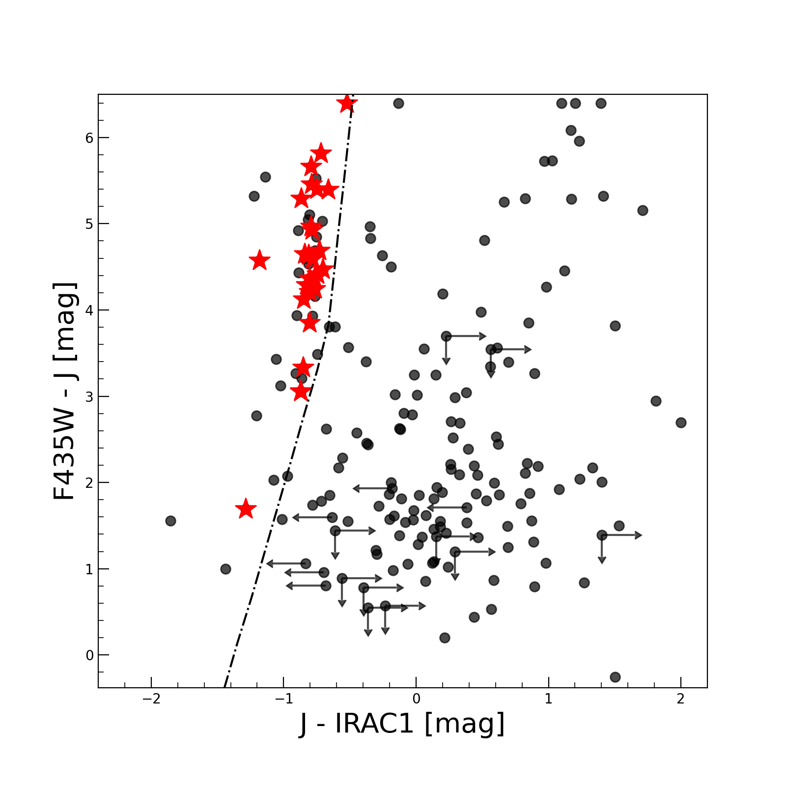
Figure 14: The color-color diagram used for selecting stars from our HDH$\alpha$ ELG candidates. The dash line represents the star selection criteria used by Dahlen2010. ELG candidates with S/N $>2$ in the J band and IRAC1 band are plotted as filled circles in this figure, and ELG candidates spectroscopically confirmed as stars are highlighted as red asterisks.

References

- Arrigoni Battaia et al. (2018) Arrigoni Battaia, F., Prochaska, J. X., Hennawi, J. F., et al. 2018, MNRAS, 473, 3907, doi: 10.1093/mnras/stx2465
- Astropy Collaboration et al. (2013) Astropy Collaboration, Robitaille, T. P., Tollerud, E. J., et al. 2013, A&A, 558, A33, doi: 10.1051/0004-6361/201322068
- Astropy Collaboration et al. (2018) Astropy Collaboration, Price-Whelan, A. M., Sipőcz, B. M., et al. 2018, AJ, 156, 123, doi: 10.3847/1538-3881/aabc4f
- Bacon et al. (2022) Bacon, R., Brinchmann, J., Conseil, S., et al. 2022, arXiv e-prints, arXiv:2211.08493. https://arxiv.org/abs/2211.08493
- Balestra et al. (2010) Balestra, I., Mainieri, V., Popesso, P., et al. 2010, A&A, 512, A12, doi: 10.1051/0004-6361/200913626
- Beckwith et al. (2006) Beckwith, S. V. W., Stiavelli, M., Koekemoer, A. M., et al. 2006, AJ, 132, 1729, doi: 10.1086/507302
- Benitez et al. (2014) Benitez, N., Dupke, R., Moles, M., et al. 2014, arXiv e-prints, arXiv:1403.5237. https://arxiv.org/abs/1403.5237
- Bertin (2010) Bertin, E. 2010, Astrophysics Source Code Library, ascl:1010.068. https://ui.adsabs.harvard.edu/abs/2010ascl.soft10068B
- Bertin & Arnouts (1996) Bertin, E., & Arnouts, S. 1996, Astronomy and Astrophysics Supplement Series, 117, 393, doi: 10.1051/aas:1996164
- Bohlin (2016) Bohlin, R. C. 2016, AJ, 152, 60, doi: 10.3847/0004-6256/152/3/60
- Bond et al. (2010) Bond, N. A., Feldmeier, J. J., Matković, A., et al. 2010, ApJ, 716, L200, doi: 10.1088/2041-8205/716/2/L200
- Bouwens et al. (2022) Bouwens, R. J., Illingworth, G., Ellis, R. S., et al. 2022, arXiv e-prints, arXiv:2203.14978. https://arxiv.org/abs/2203.14978
- Bouwens et al. (2006) Bouwens, R. J., Illingworth, G. D., Blakeslee, J. P., & Franx, M. 2006, ApJ, 653, 53, doi: 10.1086/498733
- Bouwens et al. (2008) Bouwens, R. J., Illingworth, G. D., Franx, M., & Ford, H. 2008, ApJ, 686, 230, doi: 10.1086/590103
- Bouwens et al. (2004) Bouwens, R. J., Illingworth, G. D., Thompson, R. I., et al. 2004, ApJ, 606, L25, doi: 10.1086/421016
- Bouwens et al. (2010) Bouwens, R. J., Illingworth, G. D., Oesch, P. A., et al. 2010, ApJ, 709, L133, doi: 10.1088/2041-8205/709/2/L133
- Bouwens et al. (2011) —. 2011, ApJ, 737, 90, doi: 10.1088/0004-637X/737/2/90
- Bouwens et al. (2015) —. 2015, ApJ, 803, 34, doi: 10.1088/0004-637X/803/1/34
- Bradley et al. (2021) Bradley, L., Sipőcz, B., Robitaille, T., et al. 2021, astropy/photutils: 1.1.0, 1.1.0, Zenodo, doi: 10.5281/zenodo.4624996
- Brammer et al. (2012) Brammer, G. B., Sánchez-Janssen, R., Labbé, I., et al. 2012, The Astrophysical Journal, 758, L17, doi: 10.1088/2041-8205/758/1/L17
- Bunker et al. (2003) Bunker, A. J., Stanway, E. R., Ellis, R. S., McMahon, R. G., & McCarthy, P. J. 2003, MNRAS, 342, L47, doi: 10.1046/j.1365-8711.2003.06664.x
- Cai et al. (2017a) Cai, Z., Fan, X., Yang, Y., et al. 2017a, ApJ, 837, 71, doi: 10.3847/1538-4357/aa5d14
- Cai et al. (2017b) Cai, Z., Fan, X., Bian, F., et al. 2017b, ApJ, 839, 131, doi: 10.3847/1538-4357/aa6a1a
- Cantalupo et al. (2014) Cantalupo, S., Arrigoni-Battaia, F., Prochaska, J. X., Hennawi, J. F., & Madau, P. 2014, Nature, 506, 63, doi: 10.1038/nature12898
- Cowie & Hu (1998) Cowie, L. L., & Hu, E. M. 1998, AJ, 115, 1319, doi: 10.1086/300309
- Cristiani et al. (2000) Cristiani, S., Appenzeller, I., Arnouts, S., et al. 2000, A&A, 359, 489. https://arxiv.org/abs/astro-ph/0004213
- Croom et al. (2001) Croom, S. M., Warren, S. J., & Glazebrook, K. 2001, MNRAS, 328, 150, doi: 10.1046/j.1365-8711.2001.04846.x
- Decarli et al. (2012) Decarli, R., Walter, F., Yang, Y., et al. 2012, ApJ, 756, 150, doi: 10.1088/0004-637X/756/2/150
- Dickinson et al. (2004) Dickinson, M., Stern, D., Giavalisco, M., et al. 2004, ApJ, 600, L99, doi: 10.1086/381119
- Doherty et al. (2005) Doherty, M., Bunker, A. J., Ellis, R. S., & McCarthy, P. J. 2005, MNRAS, 361, 525, doi: 10.1111/j.1365-2966.2005.09191.x
- Ferreras et al. (2009) Ferreras, I., Pasquali, A., Malhotra, S., et al. 2009, ApJ, 706, 158, doi: 10.1088/0004-637X/706/1/158
- Finkelstein et al. (2008) Finkelstein, S. L., Rhoads, J. E., Malhotra, S., Grogin, N., & Wang, J. 2008, ApJ, 678, 655, doi: 10.1086/525272
- Finkelstein et al. (2011) Finkelstein, S. L., Cohen, S. H., Windhorst, R. A., et al. 2011, The Astrophysical Journal, 735, 5, doi: 10.1088/0004-637X/735/1/5
- Fu et al. (2021) Fu, S. W., Weisz, D. R., Starkenburg, E., et al. 2021, arXiv e-prints, arXiv:2111.00045. https://arxiv.org/abs/2111.00045
- Galametz et al. (2013) Galametz, A., Grazian, A., Fontana, A., et al. 2013, The Astrophysical Journal Supplement Series, 206, 10, doi: 10.1088/0067-0049/206/2/10
- Garilli et al. (2021) Garilli, B., McLure, R., Pentericci, L., et al. 2021, Astronomy & Astrophysics, 647, A150, doi: 10.1051/0004-6361/202040059
- Giavalisco et al. (2004) Giavalisco, M., Ferguson, H. C., Koekemoer, A. M., et al. 2004, The Astrophysical Journal, 600, L93, doi: 10.1086/379232
- Gonzaga et al. (2012) Gonzaga, S., Hack, W., Fruchter, A., & Mack, J. 2012, The DrizzlePac Handbook
- Górski et al. (2005) Górski, K. M., Hivon, E., Banday, A. J., et al. 2005, ApJ, 622, 759, doi: 10.1086/427976
- Grogin et al. (2011) Grogin, N. A., Kocevski, D. D., Faber, S. M., et al. 2011, The Astrophysical Journal Supplement Series, 197, 35, doi: 10.1088/0067-0049/197/2/35
- Guo et al. (2013) Guo, Y., Ferguson, H. C., Giavalisco, M., et al. 2013, The Astrophysical Journal Supplement Series, 207, 24, doi: 10.1088/0067-0049/207/2/24
- Harish et al. (2022) Harish, S., Wold, I. G. B., Malhotra, S., et al. 2022, ApJ, 934, 167, doi: 10.3847/1538-4357/ac7cf1
- Harris et al. (2020) Harris, C. R., Millman, K. J., van der Walt, S. J., et al. 2020, Nature, 585, 357, doi: 10.1038/s41586-020-2649-2
- Hayashi et al. (2018) Hayashi, M., Tanaka, M., Shimakawa, R., et al. 2018, PASJ, 70, S17, doi: 10.1093/pasj/psx088
- Hennawi et al. (2015) Hennawi, J. F., Prochaska, J. X., Cantalupo, S., & Arrigoni-Battaia, F. 2015, Science, 348, 779, doi: 10.1126/science.aaa5397
- Hu et al. (2017) Hu, W., Wang, J., Zheng, Z.-Y., et al. 2017, ApJ, 845, L16, doi: 10.3847/2041-8213/aa8401
- Hu et al. (2019) —. 2019, ApJ, 886, 90, doi: 10.3847/1538-4357/ab4cf4
- Hu et al. (2021) Hu, W., Wang, J., Infante, L., et al. 2021, Nature Astronomy, 5, 485, doi: 10.1038/s41550-020-01291-y
- Hunter (2007) Hunter, J. D. 2007, Computing in Science & Engineering, 9, 90, doi: 10.1109/MCSE.2007.55
- Illingworth et al. (2016) Illingworth, G., Magee, D., Bouwens, R., et al. 2016, arXiv e-prints, arXiv:1606.00841. https://arxiv.org/abs/1606.00841
- Illingworth et al. (2013) Illingworth, G. D., Magee, D., Oesch, P. A., et al. 2013, ApJS, 209, 6, doi: 10.1088/0067-0049/209/1/6
- Ishigaki et al. (2018) Ishigaki, M., Kawamata, R., Ouchi, M., et al. 2018, ApJ, 854, 73, doi: 10.3847/1538-4357/aaa544
- Jiang et al. (2018) Jiang, L., Wu, J., Bian, F., et al. 2018, Nature Astronomy, 2, 962, doi: 10.1038/s41550-018-0587-9
- Kashikawa et al. (2011) Kashikawa, N., Shimasaku, K., Matsuda, Y., et al. 2011, ApJ, 734, 119, doi: 10.1088/0004-637X/734/2/119
- Khostovan et al. (2015) Khostovan, A. A., Sobral, D., Mobasher, B., et al. 2015, MNRAS, 452, 3948, doi: 10.1093/mnras/stv1474
- Khostovan et al. (2020) Khostovan, A. A., Malhotra, S., Rhoads, J. E., et al. 2020, MNRAS, 493, 3966, doi: 10.1093/mnras/staa175
- Koekemoer et al. (2011) Koekemoer, A. M., Faber, S. M., Ferguson, H. C., et al. 2011, ApJS, 197, 36, doi: 10.1088/0067-0049/197/2/36
- Koekemoer et al. (2013) Koekemoer, A. M., Ellis, R. S., McLure, R. J., et al. 2013, ApJS, 209, 3, doi: 10.1088/0067-0049/209/1/3
- Kramida et al. (2022) Kramida, A., Yu. Ralchenko, Reader, J., & and NIST ASD Team. 2022, NIST Atomic Spectra Database (ver. 5.10), [Online]. Available: https://physics.nist.gov/asd [2022, November 13]. National Institute of Standards and Technology, Gaithersburg, MD.
- Kron (1980) Kron, R. G. 1980, ApJS, 43, 305, doi: 10.1086/190669
- Kurk et al. (2013) Kurk, J., Cimatti, A., Daddi, E., et al. 2013, A&A, 549, A63, doi: 10.1051/0004-6361/201117847
- Larsson et al. (2013) Larsson, J., Fransson, C., Kjaer, K., et al. 2013, ApJ, 768, 89, doi: 10.1088/0004-637X/768/1/89
- Le Fèvre et al. (2005) Le Fèvre, O., Vettolani, G., Garilli, B., et al. 2005, A&A, 439, 845, doi: 10.1051/0004-6361:20041960
- Lim et al. (2020) Lim et al. 2020, stsynphot: synphot for HST and JWST. http://ascl.net/2010.003
- Lotz et al. (2017) Lotz, J. M., Koekemoer, A., Coe, D., et al. 2017, ApJ, 837, 97, doi: 10.3847/1538-4357/837/1/97
- Luo et al. (2017) Luo, B., Brandt, W. N., Xue, Y. Q., et al. 2017, ApJS, 228, 2, doi: 10.3847/1538-4365/228/1/2
- Mack (2015) Mack, J. 2015, Combining WFC3 Mosaics of M16 with DrizzlePac, Instrument Science Report WFC3 2015-09, 22 pages
- Madau et al. (1996) Madau, P., Ferguson, H. C., Dickinson, M. E., et al. 1996, MNRAS, 283, 1388, doi: 10.1093/mnras/283.4.1388
- Malhotra & Rhoads (2002) Malhotra, S., & Rhoads, J. E. 2002, ApJ, 565, L71, doi: 10.1086/338980
- McLeod et al. (2016) McLeod, D. J., McLure, R. J., & Dunlop, J. S. 2016, MNRAS, 459, 3812, doi: 10.1093/mnras/stw904
- Mignoli et al. (2005) Mignoli, M., Cimatti, A., Zamorani, G., et al. 2005, A&A, 437, 883, doi: 10.1051/0004-6361:20042434
- Momcheva et al. (2016) Momcheva, I. G., Brammer, G. B., van Dokkum, P. G., et al. 2016, ApJS, 225, 27, doi: 10.3847/0067-0049/225/2/27
- Momose et al. (2014) Momose, R., Ouchi, M., Nakajima, K., et al. 2014, MNRAS, 442, 110, doi: 10.1093/mnras/stu825
- Momose et al. (2016) —. 2016, MNRAS, 457, 2318, doi: 10.1093/mnras/stw021
- Oesch et al. (2013) Oesch, P. A., Bouwens, R. J., Illingworth, G. D., et al. 2013, ApJ, 773, 75, doi: 10.1088/0004-637X/773/1/75
- Oesch et al. (2014) —. 2014, ApJ, 786, 108, doi: 10.1088/0004-637X/786/2/108
- Oesch et al. (2018) Oesch, P. A., Montes, M., Reddy, N., et al. 2018, ApJS, 237, 12, doi: 10.3847/1538-4365/aacb30
- Oke & Gunn (1983) Oke, J. B., & Gunn, J. E. 1983, The Astrophysical Journal, 266, 713, doi: 10.1086/160817
- Ouchi et al. (2008) Ouchi, M., Shimasaku, K., Akiyama, M., et al. 2008, ApJS, 176, 301, doi: 10.1086/527673
- Ouchi et al. (2010) Ouchi, M., Shimasaku, K., Furusawa, H., et al. 2010, ApJ, 723, 869, doi: 10.1088/0004-637X/723/1/869
- Ouchi et al. (2018) Ouchi, M., Harikane, Y., Shibuya, T., et al. 2018, PASJ, 70, S13, doi: 10.1093/pasj/psx074
- Partridge & Peebles (1967) Partridge, R. B., & Peebles, P. J. E. 1967, ApJ, 147, 868, doi: 10.1086/149079
- Pirzkal et al. (2013) Pirzkal, N., Rothberg, B., Ly, C., et al. 2013, ApJ, 772, 48, doi: 10.1088/0004-637X/772/1/48
- Popesso et al. (2009) Popesso, P., Dickinson, M., Nonino, M., et al. 2009, A&A, 494, 443, doi: 10.1051/0004-6361:200809617
- Ravikumar et al. (2007) Ravikumar, C. D., Puech, M., Flores, H., et al. 2007, A&A, 465, 1099, doi: 10.1051/0004-6361:20065358
- Rhoads et al. (2000) Rhoads, J. E., Malhotra, S., Dey, A., et al. 2000, The Astrophysical Journal, 545, L85, doi: 10.1086/317874
- Silverman et al. (2010) Silverman, J. D., Mainieri, V., Salvato, M., et al. 2010, ApJS, 191, 124, doi: 10.1088/0067-0049/191/1/124
- Skelton et al. (2014) Skelton, R. E., Whitaker, K. E., Momcheva, I. G., et al. 2014, The Astrophysical Journal Supplement Series, 214, 24, doi: 10.1088/0067-0049/214/2/24
- Sobral et al. (2013) Sobral, D., Smail, I., Best, P. N., et al. 2013, Monthly Notices of the Royal Astronomical Society, 428, 1128, doi: 10.1093/mnras/sts096
- Sobral et al. (2015) Sobral, D., Matthee, J., Best, P. N., et al. 2015, MNRAS, 451, 2303, doi: 10.1093/mnras/stv1076
- Stanway et al. (2004) Stanway, E. R., Glazebrook, K., Bunker, A. J., et al. 2004, ApJ, 604, L13, doi: 10.1086/383523
- Steidel et al. (1996) Steidel, C. C., Giavalisco, M., Pettini, M., Dickinson, M., & Adelberger, K. L. 1996, ApJ, 462, L17, doi: 10.1086/310029
- Strolger et al. (2004) Strolger, L.-G., Riess, A. G., Dahlen, T., et al. 2004, ApJ, 613, 200, doi: 10.1086/422901
- Szokoly et al. (2004) Szokoly, G. P., Bergeron, J., Hasinger, G., et al. 2004, ApJS, 155, 271, doi: 10.1086/424707
- Teplitz et al. (2013) Teplitz, H. I., Rafelski, M., Kurczynski, P., et al. 2013, AJ, 146, 159, doi: 10.1088/0004-6256/146/6/159
- Urrutia et al. (2019) Urrutia, T., Wisotzki, L., Kerutt, J., et al. 2019, Astronomy and Astrophysics, 624, A141, doi: 10.1051/0004-6361/201834656
- van der Wel et al. (2004) van der Wel, A., Franx, M., van Dokkum, P. G., & Rix, H. W. 2004, ApJ, 601, L5, doi: 10.1086/381887
- Vanzella et al. (2008) Vanzella, E., Cristiani, S., Dickinson, M., et al. 2008, A&A, 478, 83, doi: 10.1051/0004-6361:20078332
- Virtanen et al. (2020) Virtanen, P., Gommers, R., Oliphant, T. E., et al. 2020, Nature Methods, 17, 261, doi: 10.1038/s41592-019-0686-2
- Whitaker et al. (2019) Whitaker, K. E., Ashas, M., Illingworth, G., et al. 2019, The Astrophysical Journal Supplement Series, 244, 16, doi: 10.3847/1538-4365/ab3853
- Williams et al. (1996) Williams, R. E., Blacker, B., Dickinson, M., et al. 1996, AJ, 112, 1335, doi: 10.1086/118105
- Windhorst et al. (2011) Windhorst, R. A., Cohen, S. H., Hathi, N. P., et al. 2011, The Astrophysical Journal Supplement Series, 193, 27, doi: 10.1088/0067-0049/193/2/27
- Wold et al. (2021) Wold, I. G. B., Malhotra, S., Rhoads, J., et al. 2021, arXiv e-prints, arXiv:2105.12191. https://arxiv.org/abs/2105.12191
- Zheng et al. (2021) Zheng, X. Z., Cai, Z., An, F. X., Fan, X., & Shi, D. D. 2021, MNRAS, 500, 4354, doi: 10.1093/mnras/staa2882
- Zheng et al. (2016) Zheng, Z.-Y., Malhotra, S., Rhoads, J. E., et al. 2016, ApJS, 226, 23, doi: 10.3847/0067-0049/226/2/23
- Zheng et al. (2013) Zheng, Z.-Y., Finkelstein, S. L., Finkelstein, K., et al. 2013, Monthly Notices of the Royal Astronomical Society, 431, 3589, doi: 10.1093/mnras/stt440
- Zheng et al. (2017) Zheng, Z.-Y., Wang, J., Rhoads, J., et al. 2017, The Astrophysical Journal, 842, L22, doi: 10.3847/2041-8213/aa794f
- Zonca et al. (2019) Zonca, A., Singer, L., Lenz, D., et al. 2019, Journal of Open Source Software, 4, 1298, doi: 10.21105/joss.01298