Conditional Stochastic Interpolation for
Generative Learning

Abstract

We propose a conditional stochastic interpolation (CSI) approach to learning conditional distributions. CSI learns probability flow equations or stochastic differential equations that transport a reference distribution to the target conditional distribution. This is achieved by first learning the drift function and the conditional score function based on conditional stochastic interpolation, which are then used to construct a deterministic process governed by an ordinary differential equation or a diffusion process for conditional sampling. In our proposed CSI model, we incorporate an adaptive diffusion term to address the instability issues arising during the training process. We provide explicit forms of the conditional score function and the drift function in terms of conditional expectations under mild conditions, which naturally lead to an nonparametric regression approach to estimating these functions. Furthermore, we establish non-asymptotic error bounds for learning the target conditional distribution via conditional stochastic interpolation in terms of KL divergence, taking into account the neural network approximation error. We illustrate the application of CSI on image generation using a benchmark image dataset.

Abstract

In this Supplement, we provide proofs for the main results and technical lemmas.

, , and

1 Introduction

In recent years, there have been important advances in statistical modeling and analysis of high-dimensional data using a generative learning approach with deep neural networks. For example, for learning (unconditional) distributions of high-dimensional data arising in image analysis and natural language processing, the generative adversarial networks (GANs) (Goodfellow et al., 2014; Arjovsky, Chintala and Bottou, 2017) have proven to be effective and achieved impressive success (Reed et al., 2016; Zhu et al., 2017). Instead of estimating the functional forms of density functions, GANs start from a known reference distribution and learn a map that pushes the reference distribution to the data distribution.

The basic ideas of GANs have also been extended to learn conditional distributions. In particular, conditional generative adversarial networks (cGANs) (Mirza and Osindero, 2014; Zhou et al., 2023) have shown to be able to generate high-quality samples under predetermined conditions. However, these adversarially trained generative models are not exempt from drawbacks, primarily the problems of training instability (Arjovsky, Chintala and Bottou, 2017; Karras, Laine and Aila, 2019) and mode collapse (Zhao et al., 2018).

Recently, process-based methods have emerged as an area of significant interest for generative modeling due to its impressive results. In contrast to estimating a generator function in GANs, it learns a transport procedure that converts a simple reference distribution into a high-dimensional target distribution. There are mainly two categories of methods: SDE-based generative models and ODE-based generative models. A notable instance of SDE-based generative modelings is diffusion models (Ho, Jain and Abbeel, 2020; Song et al., 2020; Meng et al., 2021), which have achieved impressive empirical success (Dhariwal and Nichol, 2021). This approach embeds the target density into a Gaussian density via Ornstein-Uhlenbeck (OU) process and solves a reverse-time SDE, which yields a score-based generative model. This reverse-time process is extended to the deterministic process that maintains the consistency in time-dependent distribution (Song, Meng and Ermon, 2020; Song et al., 2020; Lu et al., 2022; Lipman et al., 2022). ODE-based models also have excellent performance (Liu, Gong and Liu, 2022; Albergo and Vanden-Eijnden, 2023; Liu et al., 2023; Xu et al., 2022). Most ODE-based methods use an interpolative trajectory modeling approach (Liu, Gong and Liu, 2022; Albergo and Vanden-Eijnden, 2023; Liu et al., 2023; Lipman et al., 2022). Liu, Gong and Liu (2022) introduces the idea of utilizing a linear interpolation to connect the target distribution and a reference distribution and (Albergo and Vanden-Eijnden, 2023) further extend the interpolation to a nonlinear case.

Both the SDE and the ODE methods are known as score-based generative models. While these methods have achieved excellent performance, the process is truncated at a finite time point, which introduces bias into the reverse process and the final estimation, due to the requirement for an infinite time horizon in this method.

A recent paper by Albergo, Boffi and Vanden-Eijnden (2023) proposes to use stochastic interpolations to generate samples for estimating drift function and score functions, and then employ ODE and SDE-based generative models to transform a reference distribution to a target distribution within a finite time interval. In addition, the score and drift functions under this framework can be estimated more easily based on a quadratic loss function, instead of score matching as in the existing score based methods. They also establish the connection between the velocity field and the distribution field, along with providing an explicit form of the score function. However, the proof techniques rely on strict assumptions on the smoothness of density functions, which may not hold in practical scenarios as real-life data often exhibits multimodal distributions or the data can have support on manifolds. In addition, the problem of score function explosion in SDE generators remains unsolved.

In this work, we extend the method of Albergo, Boffi and Vanden-Eijnden (2023) and propose a conditional stochastic interpolation (CSI) approach to conditional generative learning. We show that the score and drift functions of CSI can be expressed as certain conditional expectations. Based on these expressions, we can convert nonparametric drift and score estimation problems into regression problems in the ODE/SDE models. We leverage the expressive power of deep neural networks for estimating high-dimensional conditional score and drift functions.

Our main contributions are as follows.

• We propose a conditional stochastic interpolation (CSI) approach for learning conditional distributions. The proposed CSI leads to a bias-free generative model and provides a unified conditional synthesis mechanism for both SDE-based and ODE-based generators on a finite time interval.

• We derive the explicit forms of the conditional score function and the drift in terms of conditional expectations without making restrictive smoothness assumptions, which naturally lead to the use of nonparametric regression for estimating these functions. We analyze the boundary behaviour of the drift and score functions, which is crucial for numerical solutions of ODEs or SDEs due to the random initialization for the integrand. We also incorporate an adaptive diffusion term in our proposed SDE-based generators to address the instability issues.

• We derive upper bounds for the KL divergence between the estimator of the conditional distribution and the underlying target conditional distribution for the SDE-based conditional generator.

• We provide sufficient the conditions on the interpolation process that ensure the training stability of drift and score functions. We demonstrate that our proposed CSI approach generates high-quality samples through a stable optimization-based training procedure.

The remainder of this article is organized as follows. Section 2 introduces the CSI process along with its basic properties. Section 3 describes the generative models under CSI framework. Section 5 presents the theoretical analysis of the CSI estimators. In Section 7, we examine relevant literature and outline the similarities and distinctions between our framework and existing approaches. Section 6 provides an evaluation of our proposal methods through simulation studies on image generation and reconstruction tasks with benchmark data. Finally, Section 8 concludes and discusses the study in this work. Proofs and technical details are provided in the supplementary material.

2 Conditional stochastic interpolation

In this section, we present the proposed CSI approach and its basic properties.

2.1 Definition and basic properties

Let $Y_{0}\sim\pi_{0}$ be a random vector following a known distribution $\pi_{0}$. Let $X$ be a random vector in a Borel space $\mathcal{X}$ and $Y_{1}\mid X\sim\pi^{X}_{1}$ be a random vector following the conditional distribution $\pi^{X}_{1}$ such that $Y_{0}$ is independent of $(X,Y_{1})$. CSI approach learns a conditional stochastic process by solving the ODE/SDE equations connecting the conditional distribution of $Y_{0}\mid X$ and $Y_{1}\mid X$. Noticeably, the SDE ”mapping” from a sample of $Y_{0}\mid X$ to that of $Y_{1}\mid X$ is not a deterministic function, but rather a probabilistic relation. This feature of SDE distinguishes them from deterministic generative learning methods such as GANs, where a given input yields a unique output.

Now, we give the definition of CSI.

Definition 2.1 (Conditional stochastic interpolation).

A conditional stochastic interpolation $Y_{t}\mid X$ between $\pi_{0}$ and $\pi^{X}_{1}$ is defined by

$$[Y_{t}\mid X]=\tilde{\mathcal{I}}(Y_{0},Y_{1},X,t)+\gamma(t)\boldsymbol{\eta},\quad t\in[0,1],$$ (2.1)

where $\boldsymbol{\eta}\in\mathbb{R}^{d}$ is a standard multivariate normal random vector independent of $(X,Y_{0},Y_{1})$, $\gamma$ is a real-valued function defined on $[0,1]$, and the interpolation $\tilde{\mathcal{I}}(Y_{0},Y_{1},X,t):=\mathcal{I}(Y_{0},Y_{1},t)\mid X$ between two random vectors $Y_{0}$ and $Y_{1}\mid X$ is defined by a function $\mathcal{I}:\mathbb{R}^{d}\times\mathbb{R}^{d}\times[0,1]\rightarrow\mathbb{R}^{d}$ with the following conditions:

1. The interpolation function $\mathcal{I}$ satisfies $\mathcal{I},\partial_{t}\mathcal{I}\in L^{\infty}(\mathbb{R}^{d}\times\mathbb{R}^{d}\times[0,1])$ and the boundary conditions that $\mathcal{I}(\mathbf{y}_{0},\mathbf{y}_{\mathbf{x}},0)=\mathbf{y}_{0}$ and $\mathcal{I}(\mathbf{y}_{0},\mathbf{y}_{\mathbf{x}},1)=\mathbf{y}_{\mathbf{x}}$, where $\mathbf{y}_{0}$ and $\mathbf{y}_{\mathbf{x}}$ denote the observed values of $Y_{0}$ and $Y_{1}$ conditioning on $X=\mathbf{x}$, respectively.

2. The function $\gamma$ is a differentiable function with $\dot{\gamma}\in L^{\infty}([0,1])$ and satisfies one of the following conditions:

   1. For $t\in[0,1]$, $\gamma(t)\equiv 0$;

   2. For $t\in(0,1)$, $\gamma(t)>0$ and $\gamma(t)=0$ elsewhere.

The reference random variable $Y_{0}$ is assumed to be independent of $X$ and $Y_{1}$ since the dependence would result in an artificial and meaningless relationship (transfer mapping) (Liu, Gong and Liu, 2022). We use the definition $\tilde{\mathcal{I}}(Y_{0},Y_{1},X,t):=\mathcal{I}(Y_{0},Y_{1},t)\mid X$ to emphasize the subtle association between the function ${\mathcal{I}}$ and $\tilde{\mathcal{I}}$. Specifically, we introduce the notation $\mathcal{I}$ to facilitate derivation and avoid ambiguity arising from changes of the domain of conditioned $X,$ such that $\mathcal{I}$ can adequately characterizes the relationship between the mean motion and time when discussing the transfer path in the measurable space conditional on $X$.

The first condition in Definition 2.1 on the interpolation function $\mathcal{I}$ ensures that the variable $\tilde{\mathcal{I}}(Y_{0},Y_{1},X,t)$ does not change too rapidly along the path from $Y_{0}$ at $t=0$ to $Y_{1}\mid X$ at $t=1$. In the second condition of Definition 2.1, the perturbation function $\gamma(t)$ is required non-negative and smooth to control the stability of the stochastic term at different moments. These conditions on $\mathcal{I}$ and $\gamma$ are mild compared with those in (Albergo, Boffi and Vanden-Eijnden, 2023).

A CSI process is determined by $\mathcal{I},\gamma$ and the reference distribution $\pi_{0}$. The choices of $\mathcal{I},\gamma$, and $\pi_{0}$ result in a highly flexible selection space. Specifically, when $\gamma(t)\equiv 0,$ the process defined in (2.1) degenerates into a deterministic process. In particular, the rectified flow (Liu, Gong and Liu, 2022) is a linear interpolation model with $\mathcal{I}(\mathbf{y}_{0},\mathbf{y}_{\mathbf{x}},t)=t\mathbf{y}_{\mathbf{x}}+(1-t)\mathbf{y}_{0}$ and $\gamma(t)=0$. We defer the detailed discussion on the conditional version of deterministic linear interpolation to Section 3.

Given $\mathcal{I},\gamma$, and $\pi_{0}$, CSI models learn the velocity and distribution fields of the interpolation between $Y_{0}$ and $Y_{1}\mid X,$ thereby achieving the purpose of learning the relationship between $Y_{1}$ and $X$. The proposed CSI possesses can be described by two field functions, i.e., the velocity field (or drift function) and distribution field (or score function). The drift function represents the deterministic part of the process, which captures the long-term behavior or tendency of the process. It provides information of the mean velocity for the process at each location and time. For non-degenerate CSI processes ($\gamma(t)\not\equiv 0$), the score function is defined as the gradient of the log-likelihood function of the process, and can be explicitly expressed by known quantities. It measures the sensitivity of the changes in the density function of the process. The following theorem reveals how the drift function characterizes a stochastic interpolation process.

Theorem 2.2 (Transport equation or Liouville’s equation).

Denote the time-dependent conditional density of $Y_{t}\mid X$ by $\rho^{*}(\mathbf{x},\mathbf{y},t):=\rho^{*}_{\mathbf{x}}(\mathbf{y},t):=p(Y_{t}=\mathbf{y}\mid X=\mathbf{x}):\mathcal{X}\times\mathbb{R}^{d}\times[0,1]\rightarrow[0,+\infty)$, where $p$ denotes the density function. In particular, we denote $\rho_{\mathbf{x}}^{*}(\mathbf{y},0):=\rho^{*}(\mathbf{x},\mathbf{y},0)=p(Y_{0}=\mathbf{y}\mid X=\mathbf{x})=p(Y_{0}=\mathbf{y})$. Let the drift function $\boldsymbol{b}^{*}:\mathcal{X}\times\mathbb{R}^{d}\times(0,1)\rightarrow\mathbb{R}^{d}$ be defined by

$$\boldsymbol{b}^{*}(\mathbf{x},\mathbf{y},t):=\mathbb{E}(\partial_{t}{\mathcal{I}}(Y_{0},Y_{1},t)+\dot{\gamma}(t)\boldsymbol{\eta}\mid X=\mathbf{x},Y_{t}=\mathbf{y}),$$ (2.2)

then the time-dependent conditional density $\rho^{*}$ solves the transport equation

$$\partial_{t}\rho^{*}+\nabla\cdot(\boldsymbol{b}^{*}\rho^{*})=0,$$ (2.3)

where $\partial_{t}\rho^{*}$ denotes the partial derivative of $\rho^{*}$ with respect to $t$, and $\nabla\cdot(\boldsymbol{b}^{*}\rho^{*})$ denotes the divergence of $(\boldsymbol{b}^{*}\rho^{*})$ with respect to its second input, i.e., $\nabla\cdot(\boldsymbol{b}^{*}\rho^{*})=\frac{\partial}{\partial\mathbf{y}}\cdot(\boldsymbol{b}^{*}\rho^{*})=\Sigma_{i=1}^{d}\frac{\partial}{\partial\mathbf{y}^{(i)}}(\boldsymbol{b}^{*}\rho^{*})^{(i)}$ , where $\mathbf{y}^{(i)}$ represents the $i$-th component of $\mathbf{y}$.

Theorem 2.2 is similar to a result of (Albergo, Boffi and Vanden-Eijnden, 2023), but was obtained through a different technique without making assumptions on the time-dependent density function. It shows that the time-dependent conditional density satisfies the transport equation or Liouville’s equation with regards to the drift function. This property ensures that the distribution of the conditional stochastic interpolation evolves in a consistent and predictable manner over time.

In the following, we derive the explicit form of the conditional score function. Previously, Albergo, Boffi and Vanden-Eijnden (2023) focused on deriving the non-conditional version of the conditional score function with smoothness conditions on the data density function. Here, we only need a milder condition regarding the integrability of the gradient of the conditional density. We let the symbol $\nabla$ denote the operation of taking the derivative with respect to the second input $\mathbf{y}$, unless stated otherwise.

Assumption 1.

The gradient of the conditional density $\nabla\rho^{*}(\mathbf{x},\mathbf{y},t)$ exists for all $\mathbf{x},\mathbf{y}$ and $t$ in the domain and $\nabla\rho^{*}(\mathbf{x},\cdot,t)\in L^{1}(\mathbb{R}^{d})$. The conditional expectation $\mathbb{E}[\|\tilde{\mathcal{I}}(Y_{0},Y_{1},X,t)\|_{\infty}\mid X]$ and $\mathbb{E}[\|Y_{t}\|_{\infty}\mid X]$ exist for all $t\in[0,1]$ and $X\in\mathcal{X}$.

Theorem 2.3 (Conditional score function).

Suppose Assumption 1 holds and $\gamma(t)\not\equiv 0$, then the conditional score function $\boldsymbol{s}^{*}(\mathbf{x},\mathbf{y},t):\mathcal{X}\times\mathbb{R}^{d}\times(0,1)\rightarrow\mathbb{R}^{d}$ satisfies

$$\boldsymbol{s}^{*}(\mathbf{x},\mathbf{y},t):=\nabla\log\rho^{*}(\mathbf{x},\mathbf{y},t)=-\frac{1}{\gamma(t)}\mathbb{E}\left(\boldsymbol{\eta}\mid X=\mathbf{x},Y_{t}=\mathbf{y}\right).$$ (2.4)

Based on Theorem 2.3, the score function at the boundaries can have explosive behavior as $\gamma(t)\rightarrow 0$ when $t\to 1$, where the phenomenon are observed in SDE-based models (Kim et al., 2021). The properties of the score function at the boundaries are also influenced by the reference distribution and the underlying data distribution in addition to the perturbation function $\gamma(t)$.

The follow resutls shows that the score function at the boundary $t=0$ is well-defined when the reference random variable $Y_{0}$ follows a standard multivariate Gaussian distribution.

Theorem 2.4 (Boundary problem).

Let $\pi_{0}$ be a standard multivariate normal distribution. If $\|p_{\tilde{\mathcal{I}}(Y_{0},Y_{1},\mathbf{x},t)}-p_{Y_{0}}\|_{\infty}=o(\gamma(t))$ as $t$ tends toward $0$ for given $\mathbf{x}\in\mathcal{X}$, then $\lim_{t\to 0}\boldsymbol{s}^{*}(\mathbf{x},\mathbf{y},t)$ is well-defined with

$$\boldsymbol{s}^{*}(\mathbf{x},\mathbf{y},0)=-\mathbf{y},$$

and the value of the drift function at $t=0$ is

$$\boldsymbol{b}^{*}(\mathbf{x},\mathbf{y},0)=\mathbb{E}[\partial_{t}{\mathcal{I}}(\mathbf{y},Y_{1},0)\mid X=\mathbf{x}].$$

Theorem 2.4 implies that the values of score and drift function remain safe and integrable during initialization, which is supportive for the use of numerical solvers, such as Euler-Maruyama and stochastic Runge-Kutta methods (Platen and Bruti-Liberati, 2010) to provide approximate trajectories from ODEs/SDEs. In contrast, existing methods (Liu, Gong and Liu, 2022; Albergo and Vanden-Eijnden, 2023; Lipman et al., 2022; Dao et al., 2023; Song et al., 2020) discard the integral domain near the boundary $t=0$ to avoid potential issues of infinite-valued integrals, but introduce unnecessary truncation bias. Theorem 2.4 resolves the issue by considering normal reference distribution.

The validity of Theorem 2.4 relies on the condition that $\|p_{\tilde{\mathcal{I}}(Y_{0},Y_{1},\mathbf{x},t)}-p_{Y_{0}}\|_{\infty}=o(\gamma(t))$. This condition can hold for an appropriate interpolation function $\mathcal{I}$ and a perturbation function $\gamma$. A class of appropriate $\mathcal{I}$ and $\gamma$ functions is provided in the following corollary.

Corollary 1.

Let $y_{x}$ denote a random variable satisfying $\mathbf{y}_{\mathbf{x}}\sim Y_{1}\mid X=\mathbf{x}$ and $\mathbf{y}_{0}$ follow a standard multivariate normal distribution. Suppose

$$\mathcal{I}(\mathbf{y}_{0},\mathbf{y}_{\mathbf{x}},t)=a(t)\mathbf{y}_{0}+b(t)\mathbf{y}_{\mathbf{x}},$$ (2.5)

where $a(t),b(t)$ are functions of $t$ continuous at $0$, and satisfy $|1-a(t)|=o(\gamma(t))$ and $|b(t)|=o(\gamma(t))$ as $t$ tends to $0$. If the supports of the conditional distributions of $Y_{1}\mid X=\mathbf{x}$ for every given $\mathbf{x}$ are uniformly bounded by a finite constant $B_{1}>0,$ then $\|p_{\tilde{\mathcal{I}}(Y_{0},Y_{1},\mathbf{x},t)}-p_{Y_{0}}\|_{\infty}=o(\gamma(t))$ and $\boldsymbol{s}^{*}(\mathbf{x},\mathbf{y},0)=-\mathbf{y}$.

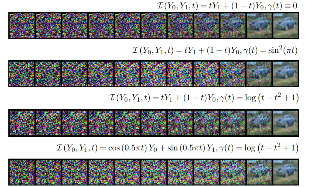
Figure 1: Examples of the interpolation function $\cal{I}$ and the perturbation function $\gamma$.

Figure 1 includes some examples of the interpolation function $\cal{I}$ and the perturbation function $\gamma$. It also displays the generating processes from white noise to an image using these interpolation and perturbation functions.

The stability of score functions at the boundary $t=0$ can be ensured under mild conditions. However, establishing the stability result of score functions at the boundary $t=1$ is more challenging. The difficulty arises from the fact that the support set of the data distribution typically resides on low-dimensional sets (Pidstrigach, 2022; De Bortoli, 2022), resulting in a drastic change of the function values of $\boldsymbol{s}$ near the boundary $t=1$. In subsection 3.2, we introduce a diffusion term to SDE samplers to mitigate this impact.

Theorems 2.2 and 2.3 give expressions of the drift and score functions in terms of conditional expectations, making it possible for their estimation in practical applications. Because of these expessions, the estimators for $\boldsymbol{b}^{*}$ and $\boldsymbol{s}^{*}$ can be obtained via nonparametric regression by minimizing a quadratic loss function.

Lemma 2.5.

The drift function $\boldsymbol{b}^{*}$ and score function $\boldsymbol{s}^{*}$ can be obtained by minimizing the corresponding loss functions,

$$\boldsymbol{b}^{*} =\operatorname*{arg\,min}_{\boldsymbol{b}}\mathcal{L}_{b}(Y_{0},Y_{1},X,\boldsymbol{\eta}),$$

$$\boldsymbol{s}^{*} =\operatorname*{arg\,min}_{\boldsymbol{s}}\mathcal{L}_{s}(Y_{0},Y_{1},X,\boldsymbol{\eta})$$

where

$$\mathcal{L}_{b}(Y_{0},Y_{1},X,\boldsymbol{\eta}) :={\displaystyle\int_{0}^{1}\mathbb{E}\|\partial_{t}{\mathcal{I}}(Y_{0},Y_{1},t)+\dot{\gamma}(t)\boldsymbol{\eta}-\boldsymbol{b}(X,Y_{t},t)\|^{2}\ \mathrm{d}t},$$ (2.6)

$$\mathcal{L}_{s}(Y_{0},Y_{1},X,\boldsymbol{\eta}) :={\displaystyle\int_{0}^{1}\mathbb{E}\|\gamma(t)^{-1}\boldsymbol{\eta}+\boldsymbol{s}(X,Y_{t},t)\|^{2}\ \mathrm{d}t},$$ (2.7)

and $Y_{t}={\mathcal{I}}(Y_{0},Y_{1},t)+\gamma(t)\boldsymbol{\eta}$.

This lemma shows that $\mathbf{b}^{*}$ and $\mathbf{s}^{*}$ can be identified as solutions to two least squares problems. This paves the way for using nonparametric regression to estimate these two functions. We will present the details in Section 4 below.

3 Conditional generators

For interpolation-type generative models, the sample $Y_{0}$ from the reference distribution is transported to the sample $Y_{1}\mid X$ from the target distribution along the conditional path $\{Y_{t}\mid X\}_{t\in[0,1]}$. By the formulated conditional interpolation process $[Y_{t}\mid X]=\tilde{\mathcal{I}}(Y_{0},Y_{1},X,t)+\gamma(t)\eta$, we can directly calculate $Y_{t}\mid X$ based on samples of $Y_{0}$ and $Y_{1}\mid X$ in a non-generative way. However, this is insufficient for generative purposes since such $Y_{t}\mid X$ does not flow along an adaptive process from the starting point $Y_{0},$ but relies on training samples of $Y_{1}\mid X$. To obtain a generator that produces new samples from $Y_{1}\mid X$, we can design ODE and SDE-based generative models, producing Markov processes $\{Z_{t}^{X}\}_{t\in[0,1]}$ with condition $X\in\mathcal{X}$ such that $Z_{0}^{X}\stackrel{{\scriptstyle d}}{{=}}Y_{0}$ and $Z_{1}^{X}\stackrel{{\scriptstyle d}}{{=}}Y_{1}\mid X$. These generative models can be constructed based on estimators of the drift function $\boldsymbol{b}^{*}$ and the score function $\boldsymbol{s}^{*}$ involved the interpolation process $Y_{t}\mid X$.

In this section, based on the stochastic interpolation procedure, we propose two conditional generators, the conditional stochastic interpolation flow (an ODE-based generative model) and the conditional stochastic interpolation process (an SDE-based generative model). These generative models under the CSI framework can be conceptualized as a two-step approach, encompassing a training step and a sampling step. In the training step, we utilize conditional stochastic interpolation to estimate the drift function $\boldsymbol{b}^{*}$ and the score function $\boldsymbol{s}^{*}$. These functions incorporate the information from $Y_{1}\mid X$ but do not directly include $Y_{1}\mid X$ as part of their inputs. This pre-sampling step enables us to capture the key characteristics of the conditional distribution without relying on explicit knowledge of $Y_{1}\mid X$. In the sampling step, we construct a Markov process $Z_{t}^{X}$, encompassing a stochastic process or the corresponding probability flow, using either the estimator of $\boldsymbol{b}^{*}$ or $\boldsymbol{s}^{*}$. The process $Z_{t}^{X}$ possesses the marginal preserving property, i.e., the time-dependent conditional distribution of $Z_{t}^{X}$ is equivalent to the interpolation $Y_{t}\mid X$, despite $Z_{t}^{X}$ and $Y_{t}\mid X$ have different transfer paths. Consequently, the solutions of the process $Z_{1}^{X}$ can serve as the generated samples from $Y_{1}\mid X$. In practice, the Euler-Maruyama and stochastic Runge-Kutta methods (Platen and Bruti-Liberati, 2010) are commonly employed for solving the corresponding ODEs/SDEs. An illustration of our CSI approach is depicted in Figure 2.

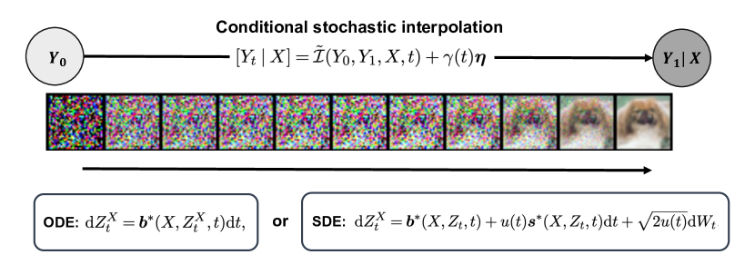
Figure 2: Illustration of the proposed CSI approach.

3.1 ODE-based generative model

We present an ODE-based generative model with conditional stochastic interpolation flow. In the training step, we first estimate the drift function by solving a simple least squares regression problem (2.6) based on samples from conditional stochastic interpolation $Y_{t}\mid X$. Once the estimator of the drift function is estimated, we can generate new samples by solving the ordinary differential equation (ODE) using the estimated drift function, which is defined in (C.1).

Definition 3.1 (Conditional stochastic interpolation flow).

Let random variables $Y_{0}\sim\pi_{0}$, and $Y_{1}\mid X\sim\pi^{X}_{1}$, where $Y_{0}\sim\pi_{0}$ is independent of $X$. The conditional stochastic flow $Z_{t}^{X}:=Z_{t}\mid X$ induced from $Y_{0}$ and $Y_{1}\mid X$ is defined by an ordinary differentiable model (ODE) over time $t\in[0,1]$,

$$\mathrm{d}Z_{t}^{X}=\boldsymbol{b}^{*}(X,Z_{t}^{X},t)\mathrm{d}t,\quad t\in[0,1].$$ (3.1)

where $Z_{0}=Y_{0}$ and the drift function $\boldsymbol{b}^{*}:\mathcal{X}\times\mathbb{R}^{d}\times[0,1]\rightarrow\mathbb{R}^{d}$ is defined as (C.1).

Equation (3.1) describes a completely deterministic motion that differs from the process (2.1). To avoid confusion, we introduce a new notation $Z_{t}$ that is different from $Y_{t}$. As a consequence of Theorem 2.2, the drift function $\boldsymbol{b}^{*}$ and the conditional density function also satisfy the Liouville’s equation ((Gardiner et al., 1985, subsection 3.5) and (Öttinger, 2012, subsection 3.3.3)), which suggests that the conditional stochastic interpolation flow converts samples of $Y_{0}$ to samples of $Y_{1}\mid X$. We present this property below.

Corollary 2.

Denote the conditional density function of the conditional stochastic interpolation flow by $\rho^{\text{ode}}(\mathbf{x},\mathbf{z},t):\mathcal{X}\times\mathbb{R}^{d}\times[0,1]\rightarrow[0,+\infty)$ defined as $\rho^{\text{ode}}(\mathbf{x},\mathbf{z},t)=\rho^{\text{ode}}_{\mathbf{x}}(\mathbf{z},t):=p(Z_{t}=\mathbf{z}\mid X=\mathbf{x})$ with $\rho^{\text{ode}}(\cdot,0)=\rho(\cdot,0)$. Then the transport equation (Liouville’s equation) holds:

$$\partial_{t}\rho^{\text{ode}}+\nabla\cdot(\boldsymbol{b}^{*}\rho^{\text{ode}})=0.$$ (3.2)

A simple example of conditional stochastic interpolation flow is the rectified flow introduced by (Liu, Gong and Liu, 2022). The rectified flow follows a linear interpolation between $Y_{0}$ and $Y_{1}$, which enhances sampling efficiency. Under the proposed CSI approach, this model is realized by setting $\mathcal{I}(\mathbf{y}_{0},\mathbf{y}_{\mathbf{x}},t)=t\mathbf{y}_{\mathbf{x}}+(1-t)\mathbf{y}_{0}$ and $\gamma(t)=0$.

Example (Conditional rectified flow).

Let random variables $Y_{0}\sim\pi_{0}$, and $Y_{1}\mid X\sim\pi^{X}_{1}$, where $Y_{0}\sim\pi_{0}$ is independent of $X$. The conditional rectified flow induced from $Y_{0}$ and $Y_{1}\mid X$ is defined by an ordinary differentiable model (ODE) over time $t\in[0,1]$,

$$\mathrm{d}Z_{t}^{X}=\boldsymbol{b}(X,Z_{t}^{X},t)\mathrm{d}t,\text{ }t\in[0,1],$$

where $Z_{0}=Y_{0}$ and the corresponding drift function $\boldsymbol{b}:\mathcal{X}\times\mathbb{R}^{d}\times[0,1]\rightarrow\mathbb{R}^{d}$ is obtain by solving the problem:

$$\min_{\boldsymbol{b}}{\displaystyle\int_{0}^{1}\mathbb{E}\|Y_{1}-Y_{0}-\boldsymbol{b}(X,Y_{t},t)\|^{2}\ \mathrm{d}t},\quad\text{with }{Y}_{t}=t{Y}_{1}+(1-t)Y_{0}.$$

3.2 SDE-based generative model

In this subsection, present the SDE-based generative model, in which a stochastic noise is included for introducing randomness and capturing the inherent uncertainty in the system being modeled. An adaptive function $u(t)$ is also incorporated to adjust the dynamic noise level during the generation process, which enhances the practicality of the model. When the adaptive function $u(t)$ is set to zero, the stochastic process degenerates into a deterministic process, i.e. the conditional stochastic interpolation flow.

Definition 3.2 (Conditional stochastic interpolation process).

Let random variables $Y_{0}\sim\pi_{0}$, and $Y_{1}\mid X\sim\pi^{X}_{1}$, where $Y_{0}\sim\pi_{0}$ is independent of $X$. The conditional stochastic process $Z_{t}^{X}:=Z_{t}\mid X$ induced from $Y_{0}$ and $Y_{1}\mid X$ is defined as

$$\mathrm{d}Z_{t}^{X}=\boldsymbol{b}_{u}(X,Z_{t}^{X},t)\mathrm{d}t+\sqrt{2u(t)}\mathrm{d}W_{t},t\in[0,1],$$ (3.3)

where $Z_{0}=Y_{0}$, $\{W_{t},t\in[0,1]\}$ is a Wiener process, and $\boldsymbol{b}_{u}(X,Z_{t},t):=\boldsymbol{b}^{*}(X,Z_{t},t)+u(t)\boldsymbol{s}^{*}(X,Z_{t},t)$ is the corresponding drift function with $\boldsymbol{b}^{*}$, $\boldsymbol{s}^{*}$ defined in (C.1) and (C.5).

The SDE-based generative models incorporate the diffusion term $\sqrt{2u(t)}\mathrm{d}W_{t}$ into the process, which differs from the model proposed in (Albergo, Boffi and Vanden-Eijnden, 2023), where the variance of noise remains constant. The diffusion function $u(t)$ in Definition 3.2 offers an enhanced flexibility and adaptability to temporal changes. With a proper adaptive diffusion function $u(t)$, the function involved in SDE process $\boldsymbol{b}_{u}(X,Z_{t},t)$ can be stabilized. Note that

$$\boldsymbol{b}_{u}(X,Z_{t},t) =\boldsymbol{b}^{*}(X,Z_{t},t)+u(t)\boldsymbol{s}^{*}(X,Z_{t},t)$$

$$=\boldsymbol{b}^{*}(X,Z_{t},t)-u(t)\frac{1}{\gamma(t)}\mathbb{E}\left(\boldsymbol{\eta}\mid X=\mathbf{x},Y_{t}=\mathbf{y}\right),$$

then setting $u(t)=\gamma(t)$ yields

$$\boldsymbol{b}_{u}(\mathbf{x},\mathbf{y},t)=\boldsymbol{b}^{*}(\mathbf{x},\mathbf{y},t)-\mathbb{E}[\boldsymbol{\eta}\mid X=\mathbf{x},Y_{t}=\mathbf{y}],$$

which is more stable when $\mathbb{E}[\boldsymbol{\eta}\mid X=\mathbf{x},Y_{t}=\mathbf{y}]$ is controllable.

The SDE given in (3.3) describes a different motion from the process (2.1). This newly generated process $Z_{t}\mid X$ is shown to satisfy the Fokker-Planck equation (Öttinger, 2012, Section 3.3.3).

Corollary 3.

Let $\rho^{\text{sde}}(\mathbf{x},\mathbf{z},t)=\rho^{\text{sde}}_{\mathbf{x}}(\mathbf{z},t):=p(Z_{t}=\mathbf{z}\mid X=\mathbf{x}):\mathcal{X}\times\mathbb{R}^{d}\times[0,1]\rightarrow[0,+\infty)$ denote the conditional density function of the process defined in (3.3) with $\rho^{\text{sde}}(\cdot,0)=\rho(\cdot,0)$. Then the Fokker-Planck equation holds, i.e.,

$$\partial_{t}\rho^{\text{sde}}+\nabla\cdot(\boldsymbol{b}_{u}\rho^{\text{sde}})-u(t)\Delta\rho^{\text{sde}}=0$$ (3.4)

for all $\mathbf{x}\in\mathcal{X}$. The symbol $\Delta$ denotes the Laplacian operator with respect to the second input.

In addition, the diffusion term makes it possible to capture the discrepancy measured by the Kullback-Leibler (KL) divergence between the estimated distribution at $t=1$ and the target distribution.

Next, we present an example of the conditional rectified flow with the specific choices of $\gamma(t)=\log(t-t^{2}+1)$ and $u(t)=1-t$. These selections provide a parametrization of the latent variable $\boldsymbol{\eta}$ and the diffusion term $\sqrt{2u(t)}\mathrm{d}W_{t}$.

Example (Conditional stochastic linear interpolation process).

Let random variables $Y_{0}\sim\pi_{0}$, and $Y_{1}\mid X\sim\pi^{X}_{1}$, where $Y_{0}\sim\pi_{0}$ is independent of $X$. A conditional stochastic linear interpolation process induced from $Y_{0}$ and $Y_{1}\mid X$ is

$$\mathrm{d}Z_{t}=\boldsymbol{b}(X,Z_{t},t)+\frac{\log^{2}(t-t^{2}+1)}{2}\boldsymbol{s}(X,Z_{t},t)\mathrm{d}t,\text{ }t\in[0,1],$$

where $Z_{0}=Y_{0}$ and the corresponding $\boldsymbol{b}$ and $\boldsymbol{s}$ can be obtained by solving the minimization problems:

$$\min_{\boldsymbol{b}}{\displaystyle\int_{0}^{1}\mathbb{E}\|Y_{1}-Y_{0}+\frac{1-2t}{t-t^{2}+1}\boldsymbol{\eta}-\boldsymbol{b}(X,Y_{t},t)\|^{2}\mathrm{d}t},$$

$$\min_{\boldsymbol{s}}{\displaystyle\int_{0}^{1}\mathbb{E}\|\frac{1}{\log(t-t^{2}+1)}\boldsymbol{\eta}+\boldsymbol{s}(X,Y_{t},t)\|^{2}\mathrm{d}t},$$

where $Y_{t}=tY_{1}+(1-t)Y_{0}+\log(t-t^{2}+1)\boldsymbol{\eta}$.

Compared with the conditional rectified flow, the inclusion of the latent variable $\gamma(t)\boldsymbol{\eta}$ and the diffusion term in this framework simplifies the structure of the intermediate density $p(Y_{t}=\mathbf{y}\mid X).$

4 Estimation of the drift and score functions

At the population level, the drift function $\mathbf{b}^{*}$ and the score function $\mathbb{s}^{*}$ can be identified over the whole interval $[0,1],$ as shown in Lemma 2.5. However, at the empirical level, it is difficult to estimate the whole processes $\{\mathbf{b}(\cdot,t),t\in[0,1]\}$ and $\{\mathbf{s}(\cdot,t),t\in[0,1]\}.$ This is particularly so for the score function $\mathbf{s}^{*}$, since its behavior at the boundary points can be unstable. Therefore, we estimate them in a pointwise manner.

For any given $t\in[0,1]$, we define respectively the $L^{2}$ risks for any $\boldsymbol{b}$ and $\boldsymbol{s}$ at time $t$ by

$$R^{b}_{t}(\boldsymbol{b}) :=\mathbb{E}\left\|\partial_{t}{\mathcal{I}}(Y_{0},Y_{1},t)+\dot{\gamma}(t)\boldsymbol{\eta}-\boldsymbol{b}(X,Y_{t},t)\right\|^{2},$$ (4.1)

$$R^{s}_{t}(\boldsymbol{s}) :=\mathbb{E}\left\|\gamma(t)^{-1}\boldsymbol{\eta}+\boldsymbol{s}(X,Y_{t},t)\right\|^{2},$$ (4.2)

where $Y_{t}=\mathcal{I}(Y_{0},Y_{1},t)+\gamma(t)\boldsymbol{\eta}$ and the expectation is taken over variables $Y_{0},(X,Y_{1}),\boldsymbol{\eta}$ that is independent of the models $\boldsymbol{b}$ and $\boldsymbol{s}$. For a fixed $t\in[0,1]$, based on the basic properties of conditional expectation, the minimums of (4.1) and (4.2) are achieved at

$$\boldsymbol{b}^{*}(\mathbf{x},\mathbf{y},t)=\mathbb{E}\left[\partial_{t}\mathcal{I}(Y_{0},Y_{1},t)+\dot{\gamma}(t)\boldsymbol{\eta}|X=\mathbf{x},Y_{t}=\mathbf{y}\right]=\arg\min_{\boldsymbol{b}}R^{b}_{t}(\boldsymbol{b}),$$ (4.3)

$$\boldsymbol{s}^{*}(\mathbf{x},\mathbf{y},t)=\mathbb{E}\left[-\gamma(t)^{-1}\boldsymbol{\eta}|X=\mathbf{x},Y_{t}=\mathbf{y}\right]=\arg\min_{\boldsymbol{s}}R^{b}_{t}(\boldsymbol{s}),$$ (4.4)

respectively for any $\mathbf{x}\in\mathcal{X}$ and $\mathbf{y}\in\mathbb{R}^{d}.$

In practice, the data distribution is usually unknown and we can not directly minimize the loss functions but the corresponding empirical risk based on a finite sample. Let $S:=\{(\mathbf{y}_{0,j},(\mathbf{x}_{1,k},\mathbf{y}_{1,k}),\boldsymbol{\eta}_{h})\}_{j,k,h}^{m,n,H}$ be a finite sample with independent and identically distributed observations drawn from the data distribution, where $n$, $m$, and $H$ correspond to the number of samples of $Y_{0}$, $(X,Y_{1})$, and $\boldsymbol{\eta}$, respectively. The sample sizes $m$, $n$, and $H$ may not be identical. It can be shown that the effective sample size of $S$ in fact depends on $\min\{m,n,H\}$ in terms of the theoretical guarantee. Without loss of generality, we set $m=n=H$ as the sample size of $S$ and rewrite the indices of the sample as $S=\{D_{k}=(\mathbf{y}_{0,k},(\mathbf{x}_{k},\mathbf{y}_{1,k}),\boldsymbol{\eta}_{k})\}_{k=1}^{n}$. Based on the effective sample $S$, for any given $t\in[0,1]$, we define the empirical risks for the drift and score functions as:

$$R_{t,n}^{b}(\boldsymbol{b}) :=\frac{1}{n}\sum_{k=1}^{n}\left\|\partial_{t}\mathcal{I}(\mathbf{y}_{0,k},\mathbf{y}_{1,k},t)+\dot{\gamma}(t)\boldsymbol{\eta}_{k}-\boldsymbol{b}(\mathbf{x}_{k},\mathbf{y}_{t,k},t)\right\|^{2},$$ (4.5)

$$R_{t,n}^{s}(\boldsymbol{s}) :=\frac{1}{n}\sum_{k=1}^{n}\left\|\gamma(t)^{-1}\boldsymbol{\eta}_{k}+\boldsymbol{s}(\mathbf{x}_{k},\mathbf{y}_{t,k},t)\right\|^{2},$$ (4.6)

where $\mathbf{y}_{t,k}=\mathcal{I}(\mathbf{y}_{0,k},\mathbf{y}_{1,k}t)+\gamma(t)\boldsymbol{\eta}_{k}$. We minimize the empirical risk over a class of neural network functions $\mathcal{F}_{n}=\{\boldsymbol{f}:\mathbb{R}^{k+d+1}\rightarrow\mathbb{R}^{d}\}$ described below.

With a finite sample $S$ and a class of functions $\mathcal{F}_{n}$, we define the empirical risk minimizer (ERM) by

$$\hat{\boldsymbol{b}}_{n}(\cdot,t)\in\arg\min_{\boldsymbol{f}\in\mathcal{F}_{n}}R_{t,n}^{b}(\boldsymbol{f}),$$ (4.7)

$$\hat{\boldsymbol{s}}_{n}(\cdot,t)\in\arg\min_{\boldsymbol{f}\in\mathcal{F}_{n}}R_{t,n}^{s}(\boldsymbol{f}),\forall t\in[0,1].$$ (4.8)

We estimate the $d$-dimensional to $d$-dimensional target functions $\boldsymbol{b}^{*}$ and $\boldsymbol{s}^{*}$ using neural networks. We consider the commonly used feedforward neural networks, the multi-layer perceptrons (MLPs). However, other types of neural networks or approximation function classes can be also be used, if their approximation error bounds are available.

A ReLU-activated multi-layer perceptron can be defined by a composited function $\boldsymbol{f}_{\boldsymbol{\theta}}:\mathbb{R}^{k+d+1}\rightarrow\mathbb{R}^{d}$ with a parameter $\boldsymbol{\theta}$:

$$\boldsymbol{f}_{\boldsymbol{\theta}}=\mathcal{L}_{\mathcal{D}}\circ\sigma\circ\mathcal{L}_{\mathcal{D}-1}\circ\sigma\circ\cdots\circ\sigma\circ\mathcal{L}_{1}\circ\sigma\circ\mathcal{L}_{0},$$

where $\sigma(x)=\max(0,x),x\in\mathbb{R}$ is the Rectified Linear Unit (ReLU) activation function applied componentwise to a vector and $\mathcal{L}_{i}(\mathbf{x})=W_{i}\mathbf{x}+\mathbf{b}_{i}$ is the $i$-th linear transformation with weight matrix $W_{i}\in\mathbb{R}^{p_{i+1}\times p_{i}}$ and bias vector $\mathbf{b}_{i}\in\mathbb{R}^{p_{i+1}}$, and $p_{i}$ is the width (the number of neurons or computational units) of the $i$-th layer for $i=0,1,\ldots,\mathcal{D}$. For MLP $\boldsymbol{f}_{\boldsymbol{\theta}}$ defined above, we let $\mathcal{D}$ denote its depth, $\mathcal{W}=\max\left\{p_{1},\ldots,p_{\mathcal{D}}\right\}$ denote its width, $\mathcal{U}=\sum_{i=1}^{\mathcal{D}}p_{i}$ denote the number of neurons, and $\mathcal{S}=\sum_{i=0}^{\mathcal{D}-1}[p_{i}\times p_{i+1}+p_{i+1}]$ denote the size. We denote the class of ReLU activated neural networks by

$$\mathcal{F}_{\mathcal{D},\mathcal{U},\mathcal{W},\mathcal{S},\mathcal{B}}:=\left\{\boldsymbol{f}_{\boldsymbol{\theta}}:W_{i}\in\mathbb{R}^{p_{i+1}\times p_{i}},\mathbf{b}_{i}\in\mathbb{R}^{p_{i+1}}{\rm\ for\ }i\in\{0,\ldots,\mathcal{D}\}{\rm\ and\ }\|\boldsymbol{f}_{\boldsymbol{\theta}}\|_{\infty}\leq\mathcal{B}\right\},$$

where $\mathcal{B}>0$ is a large constant.

Since the estimations of the target functions $\boldsymbol{b}^{*}$ and $\boldsymbol{s}^{*}$ is carried out independently, we denote the corresponding estimating neural networks by $\boldsymbol{b}_{\boldsymbol{\theta}}\in\mathcal{F}_{n}$, $\boldsymbol{s}_{\boldsymbol{\theta}^{\prime}}\in\mathcal{F}_{n}^{\prime}$, with parameters $\boldsymbol{\theta}$ and $\boldsymbol{\theta}^{\prime},$ respectively, where $\mathcal{F}_{n}:=\mathcal{F}_{\mathcal{D},\mathcal{U},\mathcal{W},\mathcal{S},\mathcal{B}}$ and $\mathcal{F}_{n}^{\prime}:=\mathcal{F}_{\mathcal{D}^{\prime},\mathcal{U}^{\prime},\mathcal{W}^{\prime},\mathcal{S}^{\prime},\mathcal{B}^{\prime}}$. For ease of presentation, we omit the subscript for the dependence of these hyperparameters on the sample size $n$ in subsequent discussions.

5 Error analysis

In this section, we consider the theoretical properties of the proposed CSI flows, including their marginal preserving properties and learning guarantees.

5.1 The marginal preserving property

In this subsection, we show that the CSI flow (ODE-based model) and process (SDE-based model) both follow the same conditional distribution of $Y_{t}\mid X=\mathbf{x}$ for all $t\in[0,1]$ and $\mathbf{x}\in\mathcal{X}$ despite their different paths, that is, the conditional distributions of these paths satisfy

$$\rho_{\mathbf{x}}(\cdot,t)=\rho_{\mathbf{x}}^{\text{ode}}(\cdot,t)=\rho_{\mathbf{x}}^{\text{sde}}(\cdot,t),\ t\in[0,1].$$

We refer to this property as the marginal preserving property, which shows the consistency and equivalence of the two approaches in capturing the conditional distributions.

Without conditioning on the covariates, the marginal preserving property for stochastic interpolations was previously proved in Albergo, Boffi and Vanden-Eijnden (2023). Here we extend the results in Albergo, Boffi and Vanden-Eijnden (2023) to the conditional stochastic interpolations under standard regularity conditions on the drift and score function of the process. First, we need the following condition that guarantees the existence and uniqueness of solutions of Fokker-Planck type equations, see, for example, Proposition 2 of (Bris and Lions, 2008).

Assumption 2.

For any $\mathbf{x}\in\mathcal{X}$, the functions $\boldsymbol{b}^{*}(\mathbf{x},\cdot,\cdot)$ and $u\boldsymbol{s}^{*}(\mathbf{x},\cdot,\cdot)$ satisfy

$$\boldsymbol{b}^{*}(\mathbf{x},\cdot,\cdot),u\boldsymbol{s}^{*}(\mathbf{x},\cdot,\cdot)\in(L^{1}(W^{1,1}_{loc}(\mathbb{R}^{d}),[0,1]))^{d},$$

$$\nabla\cdot\boldsymbol{b}^{*}(\mathbf{x},\cdot,\cdot),u\nabla\cdot\boldsymbol{s}^{*}(\mathbf{x},\cdot,\cdot)\in L^{1}(L^{\infty}(\mathbb{R}^{d}),[0,1]),$$

$$\frac{\boldsymbol{b}^{*}(\mathbf{x},\cdot,\cdot)}{1+\|\mathbf{x}\|},\frac{u\boldsymbol{s}^{*}(\mathbf{x},\cdot,\cdot)}{1+\|\mathbf{x}\|}\in(L^{1}(L^{1}+L^{\infty}(\mathbb{R}^{d}),[0,1]))^{d},$$

where $\|\cdot\|$ is the Euclidean norm, the $u(t)$ satisfies the conditions in Definition 3.2, and the local Sobolev space $W^{1,1}(\mathbb{R}^{d})$ is defined as

$$W^{1,1}_{loc}(\mathbb{R}^{d}):=\left\{f\in L^{1}_{loc}(\mathbb{R}^{d}):{D}^{\alpha}f\in L^{1}_{loc}(\mathbb{R}^{d}),\forall\|\alpha\|_{1}\leq 1\right\}.$$

Here, $L_{\mathrm{loc}}^{1}(\mathbb{R}^{d}):=\left\{f:\mathbb{R}^{d}\rightarrow\mathbb{R}\text{ measurable }:\left.f\right|_{K}\in L^{1}(K),\forall K\subset\mathbb{R}^{d},K\text{ compact }\right\}$ is locally integrable function sapce.

Lemma 5.1.

If Assumption 2 holds, then the marginal preserving property holds in the sense that $\rho^{*}=\rho^{\text{ode}}=\rho^{\text{sde}}$.

Lemma 5.1 ensures the existence and uniqueness of the density functions of the solutions to the Fokker-Planck equation. In the rest of the paper, we refer to them as $\rho^{*}.$

5.2 Learning guarantee

In this subsection, we derive learning guarantees for our proposed estimators of the drift function and the score function. We consider the upper bounds of the excess risk of the estimators. The excess risk is decomposed into stochastic error and approximation error. We derive upper bounds for these errors.

We evaluate the quality of estimator $\hat{\boldsymbol{b}}_{n}$ or $\hat{\boldsymbol{s}}_{n}$ via the corresponding excess risk, defined as the difference between the $L^{2}$ risks of ground truth and the estimator,

$$R^{b}_{t}(\hat{\boldsymbol{b}}_{n})-R^{b}_{t}(\boldsymbol{b}^{*}) =\mathbb{E}\left\|\partial_{t}\mathcal{I}(Y_{0},Y_{1},t)+\dot{\gamma}(t)\boldsymbol{\eta}-\hat{\boldsymbol{b}}_{n}(X,Y_{t},t)\right\|^{2}$$

$$\ \ \ \ -\mathbb{E}\left\|\partial_{t}\mathcal{I}(Y_{0},Y_{1},t)+\dot{\gamma}(t)\boldsymbol{\eta}-\boldsymbol{b}^{*}(X,Y_{t},t)\right\|^{2}$$

$$=\mathbb{E}\|\hat{\boldsymbol{b}}_{n}(X,Y_{t},t)-\boldsymbol{b}^{*}(X,Y_{t},t)\|^{2}$$

$$R^{s}_{t}(\hat{\boldsymbol{s}}_{n})-R^{s}_{t}(\boldsymbol{s}^{*}) =\mathbb{E}\left\|\gamma(t)^{-1}\boldsymbol{\eta}+\hat{\boldsymbol{s}}_{n}(X,Y_{t},t)\right\|^{2}-\mathbb{E}\left\|\gamma(t)^{-1}\boldsymbol{\eta}+\boldsymbol{s}^{*}(X,Y_{t},t)\right\|^{2}$$

$$=\mathbb{E}\|\hat{\boldsymbol{s}}_{n}(X,Y_{t},t)-\boldsymbol{s}^{*}(X,Y_{t},t)\|^{2}.$$

To establish upper bounds for the excess risks, following Jiao et al. (2023), we first decompose the excess risks into two parts, namely, the stochastic error and the approximation error.

Lemma 5.2.

For any $t\in[0,1]$, given random sample $S=\{D_{k}=(\mathbf{y}_{0,k},(\mathbf{x}_{k},\mathbf{y}_{1,k}),\boldsymbol{\eta}_{k})\}_{k=1}^{n}$ and two specific classes of functions $\mathcal{F}_{n}$, $\mathcal{F}_{n}^{\prime}$, we have

$$\mathbb{E}_{S}\{R^{b}_{t}(\hat{\boldsymbol{b}}_{n})-R^{b}_{t}(\boldsymbol{b}^{*})\}\leq\mathbb{E}_{S}\{R^{b}_{t}(\hat{\boldsymbol{b}}_{n})-2R_{t,n}^{b}(\hat{\boldsymbol{b}}_{n})+R^{b}_{t}(\boldsymbol{b}^{*})\}+2d\inf_{\boldsymbol{f}\in\mathcal{F}_{n}}\|\boldsymbol{b}-\boldsymbol{b}^{*}\|_{\infty}^{2}.$$

$$\mathbb{E}_{S}\{R^{s}_{t}(\hat{\boldsymbol{s}}_{n})-R^{s}_{t}(\boldsymbol{s}^{*})\}\leq\mathbb{E}_{S}\{R^{s}_{t}(\hat{\boldsymbol{s}}_{n})-2R_{t,n}^{s}(\hat{\boldsymbol{s}}_{n})+R^{s}_{t}(\boldsymbol{s}^{*})\}+2d\inf_{\boldsymbol{f}\in\mathcal{F}_{n}^{\prime}}\|\boldsymbol{s}-\boldsymbol{s}^{*}\|_{\infty}^{2},$$

where $\mathbb{E}_{S}$ means that the expectation is taken with respect to the randomness in the observations.

Lemma 5.2 shows that the excess risk can be bounded by the sum of stochastic error and approximation error. The stochastic error arises from the randomness of the sampling data, while the approximation error results from the limited representational power of the function class to the ground truth or the target function.

5.2.1 Stochastic error

To analyze the stochastic error of the estimators $\hat{\boldsymbol{b}}_{n}$ and $\hat{\boldsymbol{s}}_{n}$ with multi-dimensional output, we introduce notations for the class of functions restricted to its components. For neural networks in $\mathcal{F}_{n}$ with multi-dimensional output, for $i=1,\ldots,d$ we let $\mathcal{F}_{ni}:=\{\boldsymbol{f}^{(i)}:\mathbb{R}^{k+d+1}\rightarrow\mathbb{R}|\boldsymbol{f}\in\mathcal{F}_{n}\}$ denote the neural networks in $\mathcal{F}_{n}$ with univariate output restricted to the $i$-th component of the original output. For $i=1,\ldots,d$, we let $\tilde{\mathcal{F}}_{ni}:=\{\boldsymbol{f}^{(i)}:\mathbb{R}^{k+d+1}\rightarrow\mathbb{R}\mid\boldsymbol{f}^{(i)}{\rm\ has\ the\ same\ architecture\ as\ that\ of\ }\boldsymbol{f}^{(i)}\in\tilde{\mathcal{F}}_{ni}\}$ be the class of neural networks with the same architecture as those in $\mathcal{F}_{ni}$ with all possible weight matrices and bias vectors. It is worth noting that $\mathcal{F}_{ni}$ is correlated with $\mathcal{F}_{nj}$ for $i\not=j$ in the sense that functions in these two classes may share the same parameter in layers excluding the output one. On the contrary, $\tilde{\mathcal{F}}_{ni}$ is independent of $\tilde{\mathcal{F}}_{nj}$ for $i\not=j$. As a consequence, $\mathcal{F}_{ni}\subset\tilde{\mathcal{F}}_{ni}$ and $\mathcal{F}_{n}\subseteq\mathcal{F}_{n1}\times\ldots\times\mathcal{F}_{nd}\subset\tilde{\mathcal{F}}_{n1}\times\ldots\times\tilde{\mathcal{F}}_{nd}$. Similarly, we can define function classes $\tilde{\mathcal{F}}^{\prime}_{ni}:=\{\boldsymbol{f}^{(i)}:\mathbb{R}^{k+d+1}\rightarrow\mathbb{R}\mid\boldsymbol{f}^{(i)}{\rm\ has\ the\ same\ architecture\ as\ that\ of\ }\boldsymbol{f}^{(i)}\in\tilde{\mathcal{F}}^{\prime}_{ni}\}$ with $\mathcal{F}_{n}^{\prime}\subset\tilde{\mathcal{F}}_{n1}^{\prime}\times\ldots\times\tilde{\mathcal{F}}_{nd}^{\prime}$.

We conduct the error analysis for the target functions $\boldsymbol{b}^{*}$ and $\boldsymbol{s}^{*}$, and we assume the distribution of $\boldsymbol{\eta}$ to be a truncated normal distribution to simplify the proof, of which the definition is postponed to Appendix A in the Supplementary Material.

Assumption 3.

Assume that $\boldsymbol{\eta}$ follows the truncated normal distribution where there exits $B_{\eta}>1$ such that $\|\boldsymbol{\eta}\|_{\infty}\leq B_{\eta}$.

The function $\gamma(t)$ governs the rate of change of the stochastic perturbation and can affect the training stability of the process. To prevent significant deviations from either endpoint of the process, we place restrictions on the rate of $\gamma(t)$ declining to 0 at the boundaries $t=0$ and $t=1$ in the following.

Assumption 4.

Suppose $\gamma(t)\not\equiv 0$ and there exists $\zeta\in(0,1/5),\varepsilon\in(0,1)$, $0\leq B\leq B^{\prime}$ such that $B^{\prime}>\gamma(t)\geq t^{1/5-\zeta}$ for $t\in[0,\varepsilon)$, $\gamma(t)\geq B$ for $t\in[\varepsilon,1-\varepsilon]$, and $B^{\prime}>\gamma(t)\geq(1-t)^{1/5-\zeta}$ for $t\in(1-\varepsilon,1]$.

Next, we give upper bounds for the stochastic error of the ERM for $\boldsymbol{b}^{*}$ and $\boldsymbol{s}^{*}.$

Theorem 5.3.

Let $\boldsymbol{b}^{*}$, $\boldsymbol{s}^{*}$ be the target function defined in (4.3) and (4.4) under the conditional stochastic interpolation model. Suppose that Assumption 3, 4 holds, and $\|\partial_{t}\mathcal{I}\|_{\infty}\leq B_{I}^{\prime}$, $\|\dot{\gamma}\|_{\infty}\leq B_{\gamma}^{\prime}$ for some constants $B_{I}^{\prime},B_{\gamma}^{\prime}\geq 1$. Suppose that $\mathcal{B}\geq B_{I}^{\prime}+B_{\gamma}^{\prime}B_{\eta}$, $\mathcal{B}^{\prime}=B_{\eta}/B^{\prime}$ and $\|\boldsymbol{b}^{*(i)}\|_{\infty}\leq\mathcal{B}$, $\|\boldsymbol{s}^{*(i)}\|_{\infty}\leq\mathcal{B}^{\prime}$ for any $i=1,2,...,d$. Then for any $t\in[0,1]$, the ERMs $\hat{\boldsymbol{b}}_{n}$ and $\hat{\boldsymbol{s}}_{n}$ defined in (4.7) and (4.8) satisfy

$$\mathbb{E}_{S}\{R^{b}_{t}(\hat{\boldsymbol{b}}_{n})-2R_{t,n}^{b}(\hat{\boldsymbol{b}}_{n})+R^{b}_{t}(\boldsymbol{b}^{*})\}\leq c_{0}d\mathcal{B}^{5}\frac{\mathcal{SD}\log(\mathcal{S})}{n}$$

and

$$\mathbb{E}_{S}\{R^{s}_{t}(\hat{\boldsymbol{s}}_{n})-2R_{t,n}^{s}(\hat{\boldsymbol{s}}_{n})+R^{s}_{t}(\boldsymbol{s}^{*})\}\leq\left\{\begin{aligned} c_{0}^{\prime}dB_{\eta}^{5}\frac{\mathcal{S^{\prime}D^{\prime}}\log(\mathcal{S}^{\prime})}{n}t^{-(1-5\zeta)}&\text{, }&t\in[0,\varepsilon),\\ c_{0}^{\prime}d\left(\frac{B_{\eta}}{B}\right)^{5}\frac{\mathcal{S}^{\prime}\mathcal{D}^{\prime}\log(\mathcal{S}^{\prime})}{n}&\text{, }&t\in[\varepsilon,1-\varepsilon],\\ c_{0}^{\prime}dB_{\eta}^{5}\frac{\mathcal{S^{\prime}D^{\prime}}\log(\mathcal{S}^{\prime})}{n}(1-t)^{-(1-5\zeta)}&\text{, }&t\in(1-\varepsilon,1],\end{aligned}\right.$$

for $n\geq\max_{i=1,...,d}\{\operatorname{Pdim}(\tilde{\mathcal{F}}_{ni}),\operatorname{Pdim}(\tilde{\mathcal{F}}_{ni}^{\prime})\}/2$, where $c_{0},c_{0}^{\prime}>0$ are constants independent of $d,n,\mathcal{B},\mathcal{D},\mathcal{W},\mathcal{S},\mathcal{B}^{\prime},\mathcal{D}^{\prime},\mathcal{W}^{\prime}$ , and $\mathcal{S}^{\prime}$.

The stochastic error bound for the score function includes a time-dependent factor $t$, which reflects the difficulty of approximating real score function at different time steps. Particularly when $t$ is near the boundary, the score function can approach infinity, which poses significant challenges for the accurate estimation in practice (Kim et al., 2021; Pidstrigach, 2022). The bounds for the score function $\mathbf{s}$ are different from those in the standard nonparametric regression problems.

5.2.2 Approximation error

The approximation error is related to the expressive power of the neural networks and the properties such as smoothness of the target functions $\boldsymbol{b}^{*(i)}$, $\boldsymbol{s}^{*(i)}$, $i=1,\ldots,d$. Before presenting the result, we state the definition of $\beta$-Hölder smooth functions.

Definition 5.4.

$\beta=\lfloor\beta\rfloor+r>0,r\in(0,1]$, where $\lfloor\beta\rfloor$ denotes the largest integer strictly smaller than $\beta$ and $\mathbb{N}_{0}$ denotes the set of non-negative integers. For a finite constant $B_{0}>0$ and a bounded closed set $E\subset\mathbb{R}^{d}$, the H$\ddot{o}$lder class of functions $\mathcal{H}^{\beta}\left(E,B_{0}\right)$ is defined as

$$\mathcal{H}^{\beta}\left(E,B_{0}\right)$$

$$=\left\{f:E\rightarrow\mathbb{R},\max_{\|\alpha\|_{1}\leq\lfloor\beta\rfloor}\left\|D^{\alpha}f\right\|_{\infty}\leq B_{0},\max_{\|\alpha\|_{1}=\lfloor\beta\rfloor}\sup_{\mathbf{x}\neq\mathbf{y}}\frac{\left|D^{\alpha}f(\mathbf{x})-D^{\alpha}f(\mathbf{y})\right|}{\|\mathbf{x}-\mathbf{y}\|^{r}}\leq B_{0}\right\},$$

where $D^{\alpha}$ is the differential operator and $\alpha=(\alpha_{1},\ldots,\alpha_{d})$ is a multi-index of order $\|\alpha\|_{1}$ with

$$D^{\alpha}f=\frac{\partial^{\|\alpha\|_{1}}f}{\partial\mathbf{x}_{1}^{\alpha_{1}}\ldots\partial\mathbf{x}_{d}^{\alpha_{d}}}.$$

Theorem 5.5.

Assume there exists $N\geq B_{I}+B_{\gamma}\cdot B_{\eta}>0$ such that $\|X\|_{\infty}\leq N$. Suppose that the drift functions $\boldsymbol{b}^{*(i)}$ belongs to the H$\ddot{o}$lder class $\mathcal{H}^{\beta}\left([-N,N]^{k+d}\times[0,1],B_{0}\right)$ with $B_{0}>0$ and $\beta>0$ and $\boldsymbol{s}^{*(i)}$ belongs to the H$\ddot{o}$lder class $\mathcal{H}^{\beta^{\prime}}\left([-N,N]^{k+d}\times[0,1],B_{0}^{\prime}\right)$ with $B_{0}^{\prime}>0$ and $\beta^{\prime}>0$ for $i=1,\ldots,d$.

1. For any $U,V\in\mathbb{N}^{+}$, let $\mathcal{F}_{n}=\mathcal{F}_{\mathcal{D},\mathcal{W},\mathcal{U},\mathcal{S},\mathcal{B}}$ be a class of neural networks with width $\mathcal{W}=38(\lfloor\beta\rfloor+1)^{2}3^{(k+d+1)}(k+d+1)^{\lfloor\beta\rfloor+2}(3+\left\lceil\log_{2}U\right\rceil)U$, and depth $\mathcal{D}=21(\lfloor\beta\rfloor+1)^{2}(3+\left\lceil\log_{2}V\right\rceil)V+2(k+d+1)$, then

   $$\inf_{\boldsymbol{f}\in\mathcal{F}_{n}}\|\boldsymbol{f}-\boldsymbol{b}^{*}\|_{\infty}\leq 19B_{0}(\lfloor\beta\rfloor+1)^{2}(k+d+1)^{\lfloor\beta\rfloor+(\beta\vee 1)/2}(UV)^{-2\beta/(k+d+1)}.$$

2. For any $U^{\prime},V^{\prime}\in\mathbb{N}^{+}$, let $\mathcal{F}_{n}^{\prime}=\mathcal{F}^{\prime}_{\mathcal{D}^{\prime},\mathcal{W}^{\prime},\mathcal{U}^{\prime},\mathcal{S}^{\prime},\mathcal{B}^{\prime}}$ be a class of neural networks with width $\mathcal{W}^{\prime}=38(\lfloor\beta^{\prime}\rfloor+1)^{2}3^{(k+d+1)}(k+d+1)^{\lfloor\beta^{\prime}\rfloor+2}(3+\left\lceil\log_{2}U^{\prime}\right\rceil)U^{\prime}$, and depth $\mathcal{D}^{\prime}=21(\lfloor\beta^{\prime}\rfloor+1)^{2}(3+\left\lceil\log_{2}V^{\prime}\right\rceil)V^{\prime}+2(k+d+1)$, then

   $$\inf_{\boldsymbol{f}\in\mathcal{F}^{\prime}_{n}}\|\boldsymbol{f}-\boldsymbol{s}^{*}\|_{\infty}\leq 19B_{0}^{\prime}(\lfloor\beta^{\prime}\rfloor+1)^{2}(k+d+1)^{\lfloor\beta^{\prime}\rfloor+(\beta^{\prime}\vee 1)/2}(U^{\prime}V^{\prime})^{-2\beta^{\prime}/(k+d+1)}.$$

5.3 Non-asymptotic upper bound

Combining the upper bounds of stochastic error and approximation error, we can obtain the non-asymptotic upper bounds for the excess risks of the estimators $\hat{\boldsymbol{b}}_{n}$ and $\hat{\boldsymbol{s}}_{n}$.

Theorem 5.6.

Assumption 3, 4 and the conditions in Theorem 5.5 hold.

1. For any $U,V\in\mathbb{N}^{+}$, let $\mathcal{F}_{n}=\mathcal{F}_{\mathcal{D},\mathcal{W},\mathcal{U},\mathcal{S},\mathcal{B}}$ be a class of neural networks with width $\mathcal{W}=38(\lfloor\beta\rfloor+1)^{2}3^{(k+d+1)}(k+d+1)^{\lfloor\beta\rfloor+2}(3+\left\lceil\log_{2}U\right\rceil)U$, and depth $\mathcal{D}=21(\lfloor\beta\rfloor+1)^{2}(3+\left\lceil\log_{2}V\right\rceil)V+2(k+d+1)$, then for $n\geq\max_{i=1,...,d}\operatorname{Pdim}(\tilde{\mathcal{F}}_{ni})/2$ and any $t\in[0,1]$, we have

   $$\mathbb{E}_{S}\|\hat{\boldsymbol{b}}_{n}(X,Y_{t},t)-\boldsymbol{b}^{*}(X,Y_{t},t)\|^{2}$$

   $$\leq 722dB_{0}^{2}(\lfloor\beta\rfloor+1)^{4}(k+d+1)^{2\lfloor\beta\rfloor+(\beta\vee 1)}(UV)^{-4\beta/(k+d+1)}+c_{0}d\mathcal{B}^{5}\frac{\mathcal{SD}\log(\mathcal{S})}{n},$$

   where $c_{0}>0$ is a universal constant.

2. For any $U^{\prime},V^{\prime}\in\mathbb{N}^{+}$, let $\mathcal{F}_{n}^{\prime}=\mathcal{F}^{\prime}_{\mathcal{D}^{\prime},\mathcal{W}^{\prime},\mathcal{U}^{\prime},\mathcal{S}^{\prime},\mathcal{B}^{\prime}}$ be a class of neural networks with width $\mathcal{W}^{\prime}=38(\lfloor\beta^{\prime}\rfloor+1)^{2}3^{(k+d+1)}(k+d+1)^{\lfloor\beta^{\prime}\rfloor+2}(3+\left\lceil\log_{2}U^{\prime}\right\rceil)U^{\prime}$, and depth $\mathcal{D}^{\prime}=21(\lfloor\beta^{\prime}\rfloor+1)^{2}(3+\left\lceil\log_{2}V^{\prime}\right\rceil)V^{\prime}+2(k+d+1)$, then for $n\geq\max_{i=1,...,d}\operatorname{Pdim}(\tilde{\mathcal{F}}_{ni})/2$, we have

   $$\mathbb{E}_{S}\|\hat{\boldsymbol{s}}_{n}(\cdot,t)-\boldsymbol{s}^{*}(\cdot,t)\|^{2} \leq c_{0}^{\prime}dB_{\eta}^{5}\frac{\mathcal{S^{\prime}D^{\prime}}\log(\mathcal{S}^{\prime})}{n}\times\Gamma(t)$$

   $$+722dB_{0}^{\prime 2}(\lfloor\beta^{\prime}\rfloor+1)^{4}(k+d+1)^{2\lfloor\beta^{\prime}\rfloor+(\beta^{\prime}\vee 1)}(U^{\prime}V^{\prime})^{-4\beta^{\prime}/(k+d+1)},$$

   where

   $$\Gamma(t)=\left\{\begin{aligned} &t^{-(1-5\zeta_{1})},\ t\in[0,\varepsilon),\\ &1,\ t\in[\varepsilon,1-\varepsilon],\\ &(1-t)^{-(1-5\zeta)},\ t\in(1-\varepsilon,1],\end{aligned}\right.$$

and $c_{0}^{\prime}>0$ is a universal constant.

The upper bounds in Theorem 5.6 are the summations of stochastic error and approximation error. We can properly determine the network architecture with respect to $n$ and thus the trade-off between the stochastic and approximation errors to achieve the minimax optimal convergence rate for nonparametric regression (Stone, 1982).

Corollary 4.

Suppose Assumptions 3, 4 and the conditions in Theorem 5.5 hold.

1. Let $U=n^{(k+d)/(8\beta+4k+4d)}$ and $V=n^{(k+d)/(8\beta+4k+4d)}.$ t We have

   $$\mathbb{E}_{S}\|\hat{\boldsymbol{b}}_{n}(X,Y_{t},t)-\boldsymbol{b}^{*}(X,Y_{t},t)\|^{2}=O\left(n^{\frac{-2\beta}{2\beta+k+d+1}}\log^{5}n\right)$$

   for any $t\in[0,1]$.

2. Let $U^{\prime}=n^{(k+d)/(8\beta+4k+4d)}$ and $V^{\prime}=n^{(k+d)/(8\beta+4k+4d)}.$ We have

   $$\mathbb{E}_{S}\|\hat{\boldsymbol{s}}_{n}(X,Y_{t},t)-\boldsymbol{s}^{*}(X,Y_{t},t)\|^{2}=\left\{\begin{aligned} O\left(t^{-(1-5\zeta)}n^{\frac{-2\beta}{2\beta+k+d+1}}\log^{5}n\right),\quad&t\in[0,\varepsilon),\\ O\left(n^{\frac{-2\beta}{2\beta+k+d+1}}\log^{5}n\right),\quad&t\in[\varepsilon,1-\varepsilon],\\ O\left((1-t)^{-(1-5\zeta)}n^{\frac{-2\beta}{2\beta+k+d+1}}\log^{5}n\right),\quad&t\in(1-\varepsilon,1],\end{aligned}\right.$$

   where $\varepsilon=(\log n)^{-\frac{1}{1/5-\zeta}}n^{-\frac{2\beta^{\prime}}{(2\beta^{\prime}+k+d)(k+d+1)(1-5\zeta)}}$.

5.4 KL divergence

In Section 5.3, we have derived non-asymptotic upper bounds for the estimation error of the estimated drift and score functions. Naturally, a main question of interest regarding the generative models is about the quality of the generated samples. In other words, it is of interest to evaluate the accuracy of the distributions induced from the estimated score $\hat{\boldsymbol{s}}_{n}$ and the drift function $\hat{\boldsymbol{b}}_{n}$.

The error bounds for the estimators $\hat{\boldsymbol{b}}_{n}$ and $\hat{\boldsymbol{s}}_{n}$ can lead to an upper bound of the Kullback-Leibler (KL) divergence between the induced density estimator and its target. To further elucidate this connection, we first state a lemma that specifically applies to the generators under SDE-based models (the conditional stochastic interpretation process).

Lemma 5.7.

Let $\rho^{*}$ denote the solution of the Fokker-Planck equation (3.4). For any velocity ${\boldsymbol{b}}(\mathbf{x},\mathbf{z},t)$ and distribution field ${\boldsymbol{s}}(\mathbf{x},\mathbf{z},t)$, we define

$${\boldsymbol{b}}_{u}(\mathbf{x},\mathbf{z},t):={\boldsymbol{b}}(\mathbf{x},\mathbf{z},t)+u(t){\boldsymbol{s}}(\mathbf{x},\mathbf{z},t).$$

Let $Z_{t},t\in(0,1]$ be defined according to

$$\mathrm{d}Z_{t}=\boldsymbol{b}_{u}(X,Z_{t},t)\mathrm{d}t+\sqrt{2u(t)}\mathrm{d}W_{t},\qquad Z_{0}=Y_{0}.$$

We define its corresponding time-dependent conditional density ${\rho}(\mathbf{x},\mathbf{z},t):={\rho}_{\mathbf{x}}(\mathbf{z},t):=p(Z_{t}=\mathbf{z}\mid X=\mathbf{x})$ as the solution to the Fokker-Planck equation

$$\partial_{t}{{\rho}}+\nabla\cdot\left({\boldsymbol{b}}_{u}{{\rho}}\right)-u(t)\Delta{{\rho}}=0,\quad{{\rho}}(\cdot,0)=\rho^{*}(\cdot,0),$$ (5.1)

for all $\mathbf{x}\in\mathcal{X}$. Then, for any integrable functions $u$ and $u^{-1}$ and any $t\in[0,1],$ we have

$${\mathbb{E}_{\mathbf{x}}[\mathrm{KL}(\rho_{\mathbf{x}}^{*}(\cdot,t)\|{\rho}_{\mathbf{x}}(\cdot,t))]}\leq\int_{0}^{t} \frac{1}{2u(s)}\mathbb{E}\|{\boldsymbol{b}(\mathbf{x},\mathbf{z}_{s},s)}-\boldsymbol{b}^{*}(\mathbf{x},\mathbf{z}_{s},s)\|^{2}ds$$ (5.2)

$$+\int_{0}^{t}\frac{u(s)}{2}\mathbb{E}\|{\boldsymbol{s}(\mathbf{x},\mathbf{z}_{s},s)}-\boldsymbol{s}^{*}(\mathbf{x},\mathbf{z}_{s},s)\|^{2}ds.$$ (5.3)

Let $f^{*}(\mathbf{z},t):=p(Z_{t}=\mathbf{z})$ and $f(\mathbf{z}_{t},t):=\mathbb{E}_{\mathbf{x}}[\rho(\mathbf{x},\mathbf{z},t)]$ denote the corresponding density functions. Then for any $t\in(0,1],$ we have

$$\mathrm{KL}(f^{*}(\cdot,t)\|f(\cdot,t))\leq\int_{0}^{t} \frac{1}{2u(s)}\mathbb{E}\|{\boldsymbol{b}}(\mathbf{x},\mathbf{z}_{s},s)-\boldsymbol{b}^{*}(\mathbf{x},\mathbf{z}_{s},s)\|^{2}ds$$

$$+\int_{0}^{t}\frac{u(s)}{2}\mathbb{E}\|{\boldsymbol{s}}(\mathbf{x},\mathbf{z}_{s},s)-\boldsymbol{s}^{*}(\mathbf{x},\mathbf{z}_{s},s)\|^{2}ds.$$

Observing the right-hand side of the inequality (C.28) and combining it with Corollary 4, we can bound the KL divergence with respect to the sample size.

Theorem 5.8.

Let $\rho^{*}$ denote the solution of the Fokker-Planck equation (3.4). Let $\hat{\rho}_{n}$ denote the solution to the Fokker-Planck equation:

$$\partial_{t}\hat{\rho}_{n}+\nabla\cdot\left(\hat{\boldsymbol{b}}_{u,n}\hat{\rho}_{n}\right)-u(t)\Delta\hat{\rho}_{n}=0,\quad\hat{\rho}_{n}(\cdot,0)=\rho^{*}(\cdot,0),$$ (5.4)

where $\hat{\boldsymbol{b}}_{u,n}=\hat{\boldsymbol{b}}_{n}+u\hat{\boldsymbol{s}}_{n}$ is defined based on the empirical risk estimators $\hat{\boldsymbol{b}}_{n}$ and $\hat{\boldsymbol{s}}_{n}$. Suppose $u(t)t^{-(1-5\zeta)}$, $u(t)(1-t)^{-(1-5\zeta)}$ $u(t)^{-1}t^{-(1-5\zeta)}$ and $u(t)^{-1}(1-t)^{-(1-5\zeta)}$ are integrable on $[0,1]$ and suppose the conditions in Corollary 4 hold, we have

$${\mathbb{E}_{S}[\mathrm{KL}(\rho_{\mathbf{x}}^{*}(\cdot,1)\|\hat{\rho}_{n,\mathbf{x}}(\cdot,1))]}=O\left(n^{\frac{-2\beta}{2\beta+k+d+1}}\log^{5}n\right).$$

Let $\hat{f}_{n}(\mathbf{z}_{t},t):=\mathbb{E}_{\mathbf{x}}[\hat{\rho}_{n}(\mathbf{x},\mathbf{z},t)]$ denote the estimated density function, we also have

$$\mathbb{E}_{S}\left[\mathrm{KL}(f^{*}(\cdot,1)\|\hat{f}_{n}(\cdot,1))\right]=O\left(n^{\frac{-2\beta}{2\beta+k+d+1}}\log^{5}n\right)$$

for $n$ large enough.

6 Numerical examples

In this section, we use two examples to illustrate the proposed CSI in learning conditional distributions.

6.1 Conditional distribution based on a regression model

We consider the conditional distribution based on the following nonlinear regression model. We substitute the ground truth of both the drift and score functions into ODE/SDE-based generators to verify the correctness of this methodology. The regression model is

$$y_{1}=f(x)+\epsilon,$$

where $\epsilon\sim N(0,I_{d})$ and $f$ is a regression function. As an example, we take

$$f(x)=|2+(x^{(1)})^{2}/3|-|x^{(2)}|+\max\{(x^{(3)})^{3},x^{(4)}\times\exp(x^{(5)}/2)\}.$$

The reference distribution $\pi_{0}$ is set to be $N(0,I_{d})$. The interpolation function $\mathcal{I}(Y_{0},Y_{1},t)$ is $a(t)Y_{0}+b(t)Y_{1}$, with $a(t)=\cos(\pi t/2)$ and $b(t)=\sin(\pi t/2)$. The perturbation function is given by $\gamma(t)=\log(t-t^{2}+1)$. Under this setting, the drift function and the score function are

$$\boldsymbol{b}(\mathbf{x},\mathbf{y},t) =\left(\frac{\dot{a}(t)a(t)+\dot{b}(t)b(t)+\dot{\gamma}(t)\gamma(t)}{a(t)^{2}+b(t)^{2}+\gamma(t)^{2}}\right)(\mathbf{y}-b(t)f(x))+\dot{b}(t)f(x),$$

$$\boldsymbol{s}(\mathbf{x},\mathbf{y},t) =\frac{-(\mathbf{y}-b(t)f(x))}{a(t)^{2}+b(t)^{2}+\gamma(t)^{2}}.$$

The details of the derivation are given in Section C.13 of the Supplementary Material. Based on the Definitions 3.1 and 3.2, we can obtain the generators based on ODE and SDE. Additionally, the diffusion function for the SDE-based generator is defined as $u(t)=t^{2}(1-t)^{2}/8.$

To elucidate the process under various conditions, we examine two distinct conditions: $X_{0}=[0,0,0,0,0]^{T}$ and $X_{1}=[2,2,2,2,2]^{T}$ and display the conditional distributions of $Y_{t}\mid X_{0}$ and $Y_{t}\mid X_{1}$ at intermediate times $t=0.2$, $0.4$, $0.6$, and $0.8$. The sample size is $5000$. The estimated time-dependent conditional distributions based on the three process: conditional stochastic interpolation, ODE-based, and SDE-based generators are plotted in Figure 3. From the figure, the distributions of the three processes are similar at each moment. Moreover, at $t=1$, the conditional probability densities are similar. This experiment supports the result of Lemma 5.1.

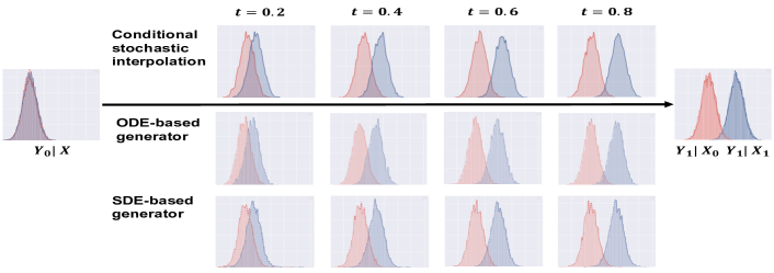
Figure 3: The sampling distribution of three processes (interpolation, flow and stochastic process) at different moments. Dashed, dotted, and solid lines represent the time-dependent distribution obtained by conditional stochastic interpolation, ODE-based generator, and SDE-based generator, respectively. The red portion represents the conditional distribution of $Y_{1}\mid X=\mathbf{0}$, and the blue portion represents the conditional distribution of $Y_{1}\mid X=2\cdot\mathbf{1}$.

6.2 The STL-10 dataset

We now illustrate the application of CSI approach to a high-dimensional data problem. Our objective is to generate images based on a given label. We provide an illustrative example using the STL-10 dataset (Coates, Ng and Lee, 2011), which contains $13,000$ images. $5,000$ images for training and $8,000$ images for testing. These images are categorized into $10$ distinct classes (e.g., airplane, bird, car, cat, deer, etc.) and the class sizes are equal. Each image is stored as a $96\times 96\times 3$ tensor for RGB channels and paired with a label in $\{0,1,...,9\}$. We use one-hot vectors in $\mathbb{R}^{10}$ to encode the ten categories. In this exercise, 10,200 images are used for training, the remaining images are reserved for final testing and evaluation.

To construct a conditional stochastic interpolation, we set the interpolation function $\mathcal{I}(Y_{0},Y_{1},t)=tY_{1}+(1-t)Y_{0}$ and the perturbation function $\gamma(t)=\sqrt{t(1-t)}$. The multivariate standard normal distribution is used as the reference distribution $\pi_{0}$. To estimate the drift function within an ODE-based generator, we employ the U-net architecture (Ronneberger, Fischer and Brox, 2015). This architecture incorporates residual blocks, upsampling blocks, downsampling blocks, and cross-attention layers (Chen, Fan and Panda, 2021) for integrating time, labels and image information. Residual blocks consist of a $3\times 3$ convolutional neural network (CNN) structure with padding of 1, while upsampling blocks and downsampling blocks employ CNN structures or nearest-neighbor interpolation for upsampling or downsampling, respectively. The model we use encompasses $10$ feature map resolutions ranging from $96\times 96$ to $6\times 6$ and the widths of networks are in sequence $(128,256,512,1024,2048,2048,1024,512,256,128)$. The shared architecture of each feature map includes two residual blocks and one function block (upsample or downsample block) , facilitating double upsampling or downsampling. Specifically, the initial five maps perform upsampling from $96\times 96$ to $6\times 6$, while the remaining five maps handle the reverse upsampling process. Due to computational limitations, attention layers are included only in the middle six feature maps (resolutions from $24\times 24$ to $6\times 6$). For training, we use the PyTorch the platform. In the sampling step, we utilize the Runge-Kutta method of order 5(4) (Dormand and Prince, 1980; Shampine, 1986) for generating approximate trajectories from the ODE. The ODE solver is provided by the Python package scipy.

As shown in Figure 4, the synthesized images closely resemble the actual ones, rendering them hard to distinguish. This suggests that CSI approach can effectively discern the distinguishing characteristics among different classes of image.

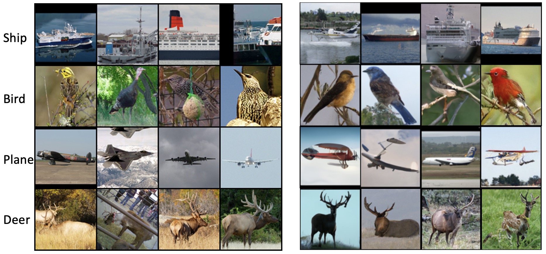
Figure 4: The real images (left panel) and the partial experimental results (right panel).

7 Related work

In this section, we discuss the connections and differences between our work and the related papers in the literature. Since there is now a big literature on process-based generative modeling approaches, it is beyond the scope of this paper to have a complete review of the existing literature, we only consider the most related ones below.

7.1 Denoising diffusion probabilistic model

Diffusion models have their roots in the concept of image denoising, known as denoising diffusion probabilistic model (DDPM) (Sohl-Dickstein et al., 2015; Ho, Jain and Abbeel, 2020). This methodology initially involves a parameterized Markov chain trained through variational inference and generates samples matching the data within a discrete time frame $\{k\}_{k=1}^{T}$, where $T\in\mathbb{N}^{+}$. Contrary to the models involved in CSI, diffusion models theoretically transport the sample $Y_{0}$ from the target distribution $\pi_{data}$ to a sample from the multivariate Gaussian distribution $\mathcal{N}(\mathbf{0},\mathbf{I}_{d})$ as time progresses from $0$ to infinity. The diffusion process or forward process $Y_{k}$ involves the incremental addition of noise to the data $Y_{0}$ according to a variance schedule $\{\beta_{1},...,\beta_{T}\}\subset\mathbb{R}^{+}$,

$$Y_{k}=\sqrt{1-\beta_{k}}Y_{k-1}+\beta_{k}\boldsymbol{\eta}.$$ (7.1)

This process can be sampled at any time step $k$ using a closed-form expression that combines the initial value $Y_{0}$ with the noise term, weighted by scaling factors $\sqrt{\bar{\alpha}_{k}}$ and $\sqrt{1-\bar{\alpha}_{k}}$:

$$Y_{k}=\sqrt{\bar{\alpha}_{k}}Y_{0}+\sqrt{1-\bar{\alpha}_{k}}\boldsymbol{\eta},\text{ with }\bar{\alpha}_{k}:=\prod_{i=1}^{k}(1-\beta_{i}).$$ (7.2)

By Tweedie’s formula (Efron, 2011), the expectation of the posterior distribution over $Y_{0}$ given $Y_{k}$ can be expressed as

$$\mathbb{E}[Y_{0}\mid Y_{k}]=\frac{1}{\sqrt{\bar{\alpha}_{k}}}Y_{k}+\frac{1-\bar{\alpha}_{k}}{\sqrt{\bar{\alpha}}_{k}}\boldsymbol{s}(Y_{k},k),$$

where the score function $\boldsymbol{s}(Y_{k},k):=\nabla_{y}\log p(Y_{k},k)$ and the symbol $\nabla_{y}$ represents the operator for taking the gradient with respect to $Y_{k}$.

Transitions of this process, denoted as $Z_{k}$, is defined as a Markov chain with learned Gaussian transitions starting at $Z_{T}\sim\mathcal{N}(\mathbf{0},\mathbf{I}_{d})$: $Z_{k-1}=\boldsymbol{\mu}_{\boldsymbol{\theta}}(Z_{k},k)+{\Sigma}_{\boldsymbol{\theta}}^{{1}/{2}}(Z_{k},k)\boldsymbol{\eta},$ where $\boldsymbol{\mu}_{\boldsymbol{\theta}}(Z_{k},k):=\frac{1}{\sqrt{1-\beta_{k}}}Z_{k}+\frac{\beta_{k}}{\sqrt{1-\beta_{k}}}\boldsymbol{s}_{\boldsymbol{\theta}}(Z_{k},k)$ and ${\Sigma}_{\boldsymbol{\theta}}:=\tilde{\beta}_{k}\mathbf{I}_{d}$. The score function $\boldsymbol{s}_{\boldsymbol{\theta}}(Z_{k},k)$ and the covariance matrix are learned through reparameterization using neural networks, with $\boldsymbol{\theta}$ representing the network parameters.

As $T$ approaches infinity, the distribution of $Y_{T}$ converges to a multivariate standard normal distribution. Therefore, in practice, it takes a large number of function evaluations to reach Casussian distribution. On the other hand, in a finite time interval, $Y_{T}$ and $Z_{T}$ are different, so there is an inevitable bias in the generative samples. Additionally, the requirement for tuning of a sequence of hyperparameters $\{\beta_{k}\}_{k=1}^{T}$ introduces unnecessary complexity and challenges in both theoretical analysis and practical implementation.

7.2 Continuous process-based generative models

The idea of using a continuous process for generative modeling was initially introduced by (Song et al., 2020). A fundamental distinction between discrete models and continuous models lies in their respective sampling approaches. DDPM employ Bayesian posterior distributions as the basis for sampling, whereas continuous models employ the inverse process of differential equations for sampling.

By defining the scale function $\beta:[0,1]\rightarrow[0,T\beta_{T}]$ as $\beta(k/T):=T\beta_{k},k\in\{0,1,...,T\}$. The equation (7.1) converges to the following stochastic differential equation (SDE) when $T\rightarrow+\infty$:

$$\mathrm{d}Y_{\tau}=-\frac{1}{2}\beta(\tau)Y_{\tau}\mathrm{d}\tau+\sqrt{\beta(\tau)}\mathrm{d}W_{\tau},\text{ }Y_{0}\sim\pi_{data},$$ (7.3)

where $W_{\tau}$ is a Wiener process for $\tau\in[0,1]$. The solution to the SDE defined in (7.3) can be expressed as a stochastic interpolation:

$$Y_{\tau}=\exp\big{(}-\frac{1}{2}\int_{0}^{\tau}\beta(s)ds\big{)}Y_{0}+\Big{[}1-\exp\big{(}-\int_{0}^{\tau}\beta(s)ds\big{)}\Big{]}^{1/2}\,\boldsymbol{\eta},\text{ }Y_{0}\sim\pi_{data}.$$ (7.4)

These models adopt a time setting that is opposite to our approach, where the time parameter ranges from $\tau=0$ to $1$, moving from the data distribution towards a reference distribution. To facilitate comparisons between different methods, we adopt the convention of using $t=1-\tau\in[0,1]$ to unify the time setting throughout the paper. Consequently, (7.4) can be rewritten as follows:

$$Y_{1-t}=\exp\big{(}-\frac{1}{2}\int_{0}^{1-t}\beta(s)ds\big{)}Y_{1}+\Big{[}1-\exp\big{(}-\int_{0}^{1-t}\beta(s)ds\big{)}\Big{]}^{1/2}\,\boldsymbol{\eta},\text{ }Y_{1}\sim\pi_{data}.$$ (7.5)

In this equation, the interpolation function and perturbation function are given by

$$\mathcal{I}(Y_{0},Y_{1},t)=\exp\big{(}-\frac{1}{2}\int_{0}^{t}\beta(s)ds\big{)}Y_{1}\ \text{ and }\ \gamma(t)=\Big{[}1-\exp(-\int_{0}^{t}\beta(s)ds\Big{]}^{1/2},$$

respectively. However, it should be noted that these functions do not satisfy the boundary conditions (1) and (2). These types of models rely on reverse SDEs for sampling, which is different from our proposed CSI approach. Specifically, for DDPM, the reverse SDE can be expressed as:

$$\mathrm{d}Z_{1-t}=\frac{1}{2}\beta(1-t)Z_{1-t}+\beta(1-t)\boldsymbol{s}_{\boldsymbol{\theta}}(Z_{1-t},1-t)\mathrm{d}t+\sqrt{\beta(1-t)}\mathrm{d}V_{1-t},$$

where $V_{1-t}$ is a reversed Wiener process. It should be noted that $Z_{1}$ and $Y_{1}$ obey different distributions, which introduces bias.

Continuous SDE-based models also suffer from low sampling efficiency due to the intractability of the time-dependent density function and the need for iterative numerical solutions to handle the reverse process. To address these challenges, deterministic samplers have been proposed, which can be derived through a deterministic ODE process known as the probability flow ODE. It has been observed in Song et al. (2020) that this approach satisfies the same Fokker-Planck equation, ensuring that it possesses the same marginal density function as the reverse SDE.

All these sampling procedures rely on the score function, which makes them known as score-based diffusion methods (SBDM). SBDM places greater emphasis on the Markov process that neglect exploring the existence solutions of reversed SDEs/ODEs of reparameterization due to the complexity associated with estimating the function $\boldsymbol{s}_{\boldsymbol{\theta}}$. Meanwhile, the numerical solution introduces bias resulting from the mismatch between the forward process $Y_{t}$ and the backward process $Z_{t}$ at time $t=1$.

In comparison, interpolation-type generative models can circumvent the bias issue of SBMDs (Albergo, Boffi and Vanden-Eijnden, 2023; Lipman et al., 2022). Liu, Gong and Liu (2022) propose a linear interpolation to connect the target distribution and a reference distribution. Albergo and Vanden-Eijnden (2023) further proposes a non-linear interpolation.

In this work, we extend the stochastic interpolation approach of Albergo, Boffi and Vanden-Eijnden (2023) to conditional process-based modeling. Our proposed CSI approach elucidates the influence of conditioning on the support set of $Y_{t}$ during the transfer, subsequently impacting the final distribution. Furthermore, because the model of Albergo, Boffi and Vanden-Eijnden (2023) uses a fixed variance scale for the stochastic term, resulting in an inevitable explosion of the score function near the data distribution and leading to truncation bias in applications, we incorporate an adaptive diffusion term (i.e., the term $\sqrt{2u(t)}$ in (3.3) in Definition 3.2) to effectively mitigate the detrimental effects of the score function explosion in the training process.

7.3 Theoretical studies of process based generative models

Theoretical studies of SBDM with SDE have aimed to establish convergence rates, assuming a given estimation error for the score function. However, these studies rely on strong assumptions concerning the data distribution, such as functional inequalities (Lee, Lu and Tan, 2022; Wibisono and Yang, 2022) or uniform Lipschitz condition (Lee, Lu and Tan, 2022; Chen et al., 2022). Some other works relax the smoothness constraint on the score function but introduce assumptions regarding infinite KL-divergence or Fisher information between the data distribution and a multivariate standard normal distribution (Chen et al., 2022; Conforti, Durmus and Silveri, 2023). Both of these conditions imply that the support of the data distribution fills the entire $\mathbb{R}^{d}$ space. Violation of this assumption leads to the explosion of score functions. Theoretical results on DDPM are limited. To the best of our knowledge, only (Li et al., 2023) derive a convergence rate for the DDPM-type sampler but it is obtained under a specific setting of hyperparameters $\{\beta_{t}\}_{t=1}^{T}$.

Under a manifold support assumption, Pidstrigach (2022) shows that the approximate backward process converges to a random variable whose distribution is supported on the manifold of interest. De Bortoli (2022) complement these results by studying the discretization scheme and providing quantitative bounds between the output of the diffusion model and the target distribution. However, these techniques either suffer from exponential dependence on problem parameters (De Bortoli, 2022) or high iteration complexity (Lee, Lu and Tan, 2023; Chen, Lee and Lu, 2023). A recent work by Benton et al. (2023) improves upon the result of Chen, Lee and Lu (2023) and obtains error bounds that are linear in the data dimension.

For interpolation based generative models, (Liu, Gong and Liu, 2022) present a derivation of the transport equation within the framework of deterministic and linear interpolation, elucidating the connection between the velocity field and the distribution field. (Chen, Daras and Dimakis, 2023) further generalize the results to encompass broader scenarios involving stochastic and nonlinear situations using Fourier transform techniques. However, their approach is constrained by the requirements of function space and smoothness conditions imposed on the data density function to ensure the validity of the inverse Fourier Transform. In contrast, we employ a different technique to obtain the transport equation and circumvent the need for these strict assumptions about data distribution.

Furthermore, we derive the closed form of the conditional score function by making reasonable $L^{1}$ integrability and finite moment assumptions. These theoretical preparations lay the groundwork for aligning the distribution transfer of stochastic interpolation with the Markov processes constructed by the corresponding drift and scoring functions, a crucial aspect in the context of interpolation-type generative models. In this aspect, it is essential to explore the existence and uniqueness of the solutions to Fokker-Planck equation (Liu, Gong and Liu, 2022). We assume the regularity condition Assumption (2) to ensure the existence and uniqueness of such solutions.

Regarding the convergence of the distribution of generated samples, the existing results were established based on pre-specified estimators of drift function and score function with a given accuracy of estimation. The upper bounds expressed in terms of the pre-sepcified estimation accuracy were derived for the ODE sampler in terms of 2-Wasserstein distance (Benton, Deligiannidis and Doucet, 2023), and the SDE sampler in terms of KL divergence (Albergo, Boffi and Vanden-Eijnden, 2023). In addition, the former work relies on a Lipschitz type condition, while the latter neglects the impact of an unstable score function near the data distribution on the transportation process, leading to an unavoidable introduction of early stopping. Our proposed CSI approach effectively mitigates the influence of score function explosion and bias resulting from imprecise transportation.

For interpolation-type models, we first provide the learning guarantee based on the neural network function class, where we establish upper bounds for both stochastic error and approximation error in the estimation of the drift and score function, respectively. The approximation capability of neural networks is linked to the smoothness of functions, and our analysis relies on this assumption solely for assessing approximation errors. It is worth highlighting that the estimation error bound for the score function depends on $t.$ Therefore, our error analysis considers the difficulty of approximating real functions at different time points, particularly when the score function approaches explosion. This aspect aligns more closely with practical scenarios, where obtaining accurate estimates at the boundary is usually more challenging. Furthermore, we establish non-asymptotic upper error bounds for the learned conditional distribution in terms of the KL divergence.

8 Conclusions and discussion

In this work, we have proposed a CSI method for conditional generative learning, which provides a unified basis for using conditional ODE-based and SDE-based models. We have provided learning guarantees for the estimation accuracy of the CSI generative models. Under mild conditions, we have established the non-asymptotic error bounds for the estimated drift and score functions based on the conditional stochastic interpolation process. In particular, we have derived an upper bound on the KL divergence between the distributions of generated samples and the truth for the SDE-based generative model.

We have also conducted numerical experiments to evaluate CSI, which show that it works well in the examples we have considered, including a nonparametric conditional density estimation problems to a more complex image generation problem. However, the scope of our numerical experiments are limited, more extensive studies with simulated and real data are needed to further examine the performance of CSI.

Several questions deserve further investigation. First, it would be of interest to derive upper bounds of the KL divergence between the sample distribution of the ODE-based generator and the underlying target distribution, in addition to the results on SDE-based models. Second, it would be beneficial to explore a weaker version of the marginal preserving property, or weaker conditions required to establish it. For generative purposes, it is enough that the sample distribution at the terminal $t=1$ of the ODE-based or SDE-based generator is consistent with the target, while marginal preserving property ensures time-dependent conditional distributions of the three processes (interpolation, flow, and stochastic process) are equivalent at each moment. Finally, extending the proposed CSI approach to infinite integral fields would be a meaningful endeavor since score-based diffusion models can be regarded as a variant in CSI framework, namely the infinite-horizon conditional stochastic interpolation. This extension would enrich the theory and improve the understanding and application of diffusion models. We leave these research questions for the future work.

Supplementary Material to “Conditional Stochastic Interpolation for Generative Learning”

Ding Huang, Jian Huang, Ting Li, Guohao Shen

Hong Kong Polytechnic University

In this supplementary material, we present technical details and proofs of the theoretical results stated in the paper.

Appendix A Definitions

Definition A.1 (Covering number).

For a given sequence $\mathbf{x}=\left(x_{1},\ldots,x_{n}\right)\in\mathcal{Y}$, let $\mathcal{F}_{n}|_{\mathbf{x}}=\{(f(x_{1}),\ldots,f(x_{n})):f\in\mathcal{F}_{n}\}$ be a subset of $\mathbb{R}^{n}$. For a positive number $\delta$, let $\mathcal{N}(\delta,\|\cdot\|_{\infty},\mathcal{F}_{n}|_{\mathbf{x}})$ denote the covering number of $\mathcal{F}_{n}|_{\mathbf{x}}$ under the norm $\|\cdot\|_{\infty}$ with radius $\delta$. Define the uniform covering number $\mathcal{N}_{n}(\delta,\|\cdot\|_{\infty},\mathcal{F}_{n})$ by the maximum of the covering number $\mathcal{N}(\delta,\|\cdot\|_{\infty},\mathcal{F}_{n}|_{\mathbf{x}})$ over all $\mathbf{x}\in\mathcal{Y}$, i.e.

$$\mathcal{N}_{n}\left(\delta,\|\cdot\|_{\infty},\mathcal{F}_{n}\right)=\max\left\{\mathcal{N}\left(\delta,\|\cdot\|_{\infty},\mathcal{F}_{n}|_{\mathbf{x}}\right):\mathbf{x}\in\mathcal{Y}\right\}.$$

Definition A.2.

Let $\mathcal{F}$ be a set of functions mapping from a domain $X$ to $\mathbb{R}$ and suppose that $S=\left\{x_{1},x_{2},\ldots,x_{m}\right\}\subseteq X$. Then $S$ is pseudo-shattered by $\mathcal{F}$ if there are real numbers $r_{1},r_{2},\ldots,r_{m}$ such that for each $b\in\{0,1\}^{m}$ there is a function $f_{b}$ in $F$ with $\operatorname{sgn}\left(f_{b}\left(x_{i}\right)-r_{i}\right)=b_{i}$ for $1\leq i\leq m$. We say that $r=\left(r_{1},r_{2},\ldots,r_{m}\right)$ witnesses the shattering.

Definition A.3 (Pseudo-dimension).

Suppose that $\mathcal{F}$ is a set of functions from a domain $X$ to $\mathbb{R}$. Then $\mathcal{F}$ has pseudo-dimension $d$ if $d$ is the maximum cardinality of a subset $S$ of $X$ that is pseudo-shattered by $\mathcal{F}$. If no such maximum exists, we say that $\mathcal{F}$ has infinite pseudo-dimension. The pseudo-dimension of $\mathcal{F}$ is denoted $\operatorname{Pdim}(\mathcal{F})$.

Definition A.4 (Truncated normal distribution).

Suppose $X\in\mathbb{R}^{d}$ follows the multivariate normal distribution with mean $\boldsymbol{\mu}$ and variance $\boldsymbol{\Sigma}$. Let $(a,b)$ be an interval with $-\infty\leq a<b\leq\infty$. Then $X$ conditional on $a<\|X\|_{\infty}<b$ has a truncated normal distribution with probability density function $f$ given by

$$f(\mathbf{x};\boldsymbol{\mu},\boldsymbol{\Sigma},a,b)=\det(\boldsymbol{\Sigma})^{-1/2}\frac{\varphi\left(\boldsymbol{\Sigma}^{-1/2}(\mathbf{x}-\boldsymbol{\mu})\right)}{\Phi\left(\boldsymbol{\Sigma}^{-1/2}(b\mathbf{1}-\boldsymbol{\mu})\right)-\Phi\left(\boldsymbol{\Sigma}^{-1/2}({a\mathbf{1}-\boldsymbol{\mu}})\right)},\ a<\|X\|_{\infty}<b$$

and $f=0$ otherwise. Here,

$$\varphi(\boldsymbol{\xi})=(2\pi)^{-2/d}\exp\left(-\frac{1}{2}\|\boldsymbol{\xi}\|^{2}\right),\boldsymbol{\xi}\in\mathbb{R}^{d}$$

is the probability density function of the multivariate standard normal distribution and $\Phi$ is its cumulative distribution function.

Appendix B Assumption

We state an assumption for the marginal preserving property. This condition guarantees the existence and uniqueness of solutions of Fokker-Planck type equations, see, for example, Proposition 2 of (Bris and Lions, 2008).

Assumption 5.

For any $\mathbf{x}\in\mathcal{X}$, the functions $\boldsymbol{b}^{*}(\mathbf{x},\cdot,\cdot)$ and $u\boldsymbol{s}^{*}(\mathbf{x},\cdot,\cdot)$ satisfy

$$\boldsymbol{b}^{*}(\mathbf{x},\cdot,\cdot),u\boldsymbol{s}^{*}(\mathbf{x},\cdot,\cdot)\in(L^{1}(W^{1,1}_{loc}(\mathbb{R}^{d}),[0,1]))^{d},$$

$$\nabla\cdot\boldsymbol{b}^{*}(\mathbf{x},\cdot,\cdot),u\nabla\cdot\boldsymbol{s}^{*}(\mathbf{x},\cdot,\cdot)\in L^{1}(L^{\infty}(\mathbb{R}^{d}),[0,1]),$$

$$\frac{\boldsymbol{b}^{*}(\mathbf{x},\cdot,\cdot)}{1+\|\mathbf{x}\|},\frac{u\boldsymbol{s}^{*}(\mathbf{x},\cdot,\cdot)}{1+\|\mathbf{x}\|}\in(L^{1}(L^{1}+L^{\infty}(\mathbb{R}^{d}),[0,1]))^{d},$$

where $\|\cdot\|$ is the Euclidean norm, the $u(t)$ satisfies the conditions in Definition 3.2, and the local Sobolev space $W^{1,1}(\mathbb{R}^{d})$ is defined as

$$W^{1,1}_{loc}(\mathbb{R}^{d}):=\left\{f\in L^{1}_{loc}(\mathbb{R}^{d}):{D}^{\alpha}f\in L^{1}_{loc}(\mathbb{R}^{d}),\forall\|\alpha\|_{1}\leq 1\right\}.$$

Here, $L_{\mathrm{loc}}^{1}(\mathbb{R}^{d}):=\left\{f:\mathbb{R}^{d}\rightarrow\mathbb{R}\text{ measurable }:\left.f\right|_{K}\in L^{1}(K),\forall K\subset\mathbb{R}^{d},K\text{ compact }\right\}$ is locally integrable function sapce.

Appendix C Proofs

For ease of reference, we first restate the results in the main text, and then give the proofs.

C.1 Proof of Theorem 2.2

Theorem 2.2. Denote the time-dependent conditional density of $Y_{t}\mid X$ by $\rho^{*}(\mathbf{x},\mathbf{y},t):=\rho^{*}_{\mathbf{x}}(\mathbf{y},t):=p(Y_{t}=\mathbf{y}\mid X=\mathbf{x}):\mathcal{X}\times\mathbb{R}^{d}\times[0,1]\rightarrow[0,+\infty)$, where $p$ denotes the density function. In particular, we denote $\rho_{\mathbf{x}}^{*}(\mathbf{y},0):=\rho^{*}(\mathbf{x},\mathbf{y},0)=p(Y_{0}=\mathbf{y}\mid X=\mathbf{x})=p(Y_{0}=\mathbf{y})$. Let the drift function $\boldsymbol{b}^{*}:\mathcal{X}\times\mathbb{R}^{d}\times(0,1)\rightarrow\mathbb{R}^{d}$ be defined by

$$\boldsymbol{b}^{*}(\mathbf{x},\mathbf{y},t):=\mathbb{E}(\partial_{t}{\mathcal{I}}(Y_{0},Y_{1},t)+\dot{\gamma}(t)\boldsymbol{\eta}\mid X=\mathbf{x},Y_{t}=\mathbf{y}),$$ (C.1)

then the time-dependent conditional density $\rho^{*}$ solves the transport equation

$$\partial_{t}\rho^{*}+\nabla\cdot(\boldsymbol{b}^{*}\rho^{*})=0,$$ (C.2)

where $\partial_{t}\rho^{*}$ denotes the partial derivative of $\rho^{*}$ with respect to $t$, and $\nabla\cdot(\boldsymbol{b}^{*}\rho^{*})$ denotes the divergence of $(\boldsymbol{b}^{*}\rho^{*})$ with respect to its second input, i.e., $\nabla\cdot(\boldsymbol{b}^{*}\rho^{*})=\frac{\partial}{\partial\mathbf{y}}\cdot(\boldsymbol{b}^{*}\rho^{*})=\Sigma_{i=1}^{d}\frac{\partial}{\partial\mathbf{y}^{(i)}}(\boldsymbol{b}^{*}\rho^{*})^{(i)}$ , where $\mathbf{y}^{(i)}$ represents the $i$-th component of $\mathbf{y}$.

Proof.

Given $X\in\mathcal{X}$, our target is to prove that the conditional density $\rho^{*}(\mathbf{x},\mathbf{y},t)$ solves the continuity equation for $\rho$:

$$\partial_{t}\rho+\nabla\cdot\left(\boldsymbol{b}\rho\right)=0,$$ (C.3)

where $\boldsymbol{b}$ is the conditional drift function. Let $\varphi:\mathbb{R}^{d}\rightarrow\mathbb{R}$ be a continuously differentiable test function with compact support. Then for any given $X\in\mathcal{X}$ and $t\in(0,1)$, we have

$$\int\left(\partial_{t}\rho^{*}+\nabla\cdot\left(\boldsymbol{b}^{*}\rho^{*}\right)\right)\varphi d\mathbf{y} =\int(\varphi\partial_{t}\rho^{*}-\nabla\varphi\cdot\boldsymbol{b}^{*}\rho^{*})d\mathbf{y}$$

$$=\partial_{t}\mathbb{E}\left[\varphi\left(Y_{t}\right)\mid X\right]-\mathbb{E}\left[\nabla\varphi\left(Y_{t}\right)\cdot\boldsymbol{b}^{*}(X,Y_{t},t)\mid X\right],$$

where the first equation follows from integration by parts that $\int\varphi\nabla\cdot\left(\boldsymbol{b}^{*}\rho^{*}\right)=-\int\nabla\varphi\cdot\boldsymbol{b}^{*}\rho^{*}$. Note that

$$\partial_{t}\mathbb{E}\left[\varphi\left(Y_{t}\right)\mid X\right]= \mathbb{E}\left[\nabla\varphi\left(Y_{t}\right)\cdot\dot{Y}_{t}\mid X\right]=\mathbb{E}\left[\nabla\varphi\left(Y_{t}\right)\cdot\mathbb{E}\left[\dot{Y}_{t}\mid X,Y_{t}\right]\mid X\right]$$ (C.4)

$$= \mathbb{E}\left[\nabla\varphi\left(Y_{t}\right)\cdot\boldsymbol{b}^{*}\left(X,Y_{t},t\right)\mid X\right],$$

where $\boldsymbol{b}^{*}(X,Y_{t},t):=\mathbb{E}\left[\dot{Y}_{t}\mid X,Y_{t}\right]$ by definition. Then

$$\int\left(\partial_{t}\rho^{*}+\nabla\cdot\left(\boldsymbol{b}^{*}\rho^{*}\right)\right)\varphi d\mathbf{y}=0$$

for any $\varphi$, which completes the proof. ∎

C.2 Proof of Theorem 2.3

Theorem 2.3 [Conditional score function]. Suppose Assumption 1 holds and $\gamma(t)\not\equiv 0$, then the conditional score function $\boldsymbol{s}^{*}(\mathbf{x},\mathbf{y},t):\mathcal{X}\times\mathbb{R}^{d}\times(0,1)\rightarrow\mathbb{R}^{d}$ satisfies

$$\boldsymbol{s}^{*}(\mathbf{x},\mathbf{y},t):=\nabla\log\rho^{*}(\mathbf{x},\mathbf{y},t)=-\frac{1}{\gamma(t)}\mathbb{E}\left(\boldsymbol{\eta}\mid X=\mathbf{x},Y_{t}=\mathbf{y}\right).$$ (C.5)

Proof.

Our proof follows Theorem 2.8 in (Albergo, Boffi and Vanden-Eijnden, 2023). Based on condition 2, we consider the case where $\gamma(t)>0$ for $t\in(0,1)$. We can utilize Gaussian integration by parts to derive the following equality:

$$\mathbb{E}\left[\boldsymbol{\eta}e^{i\gamma(t)\mathbf{v}\cdot\boldsymbol{\eta}}\right] =-\gamma(t)^{-1}\left(i\nabla_{\mathbf{v}}\right)\mathbb{E}e^{i\gamma(t)\mathbf{v}\cdot\boldsymbol{\eta}}$$

$$=-\gamma(t)^{-1}\left(i\nabla_{\mathbf{v}}\right)e^{-\frac{1}{2}\gamma^{2}(t)\|\mathbf{v}\|^{2}}$$

$$=\gamma(t)i\mathbf{v}e^{-\frac{1}{2}\gamma^{2}(t)\|\mathbf{v}\|^{2}}$$

$$=\gamma(t)i\mathbf{v}\mathbb{E}\left[e^{i\mathbf{v}\cdot\gamma(t)\boldsymbol{\eta}}\right],$$

for any $\mathbf{v}\in\mathbb{R}^{d}$ where $i=\sqrt{-1}$ is the imaginary unit. As a result, by the independence between $Y_{0},(X,Y_{1})$, and $\boldsymbol{\eta}$, for any $\mathbf{x}\in\mathcal{X}$ and $t\in(0,1)$, we have

$$\mathbb{E}\left[\boldsymbol{\eta}e^{i\mathbf{v}\cdot Y_{t}}\mid X=\mathbf{x}\right] =\mathbb{E}\left[e^{i\mathbf{v}\cdot\mathcal{I}(Y_{0},Y_{1},t)}\mid X=\mathbf{x}\right]\mathbb{E}\left[\boldsymbol{\eta}e^{i\gamma(t)\mathbf{v}\cdot\boldsymbol{\eta}}\mid X=\mathbf{x}\right]$$ (C.6)

$$=\gamma(t)i\mathbf{v}\mathbb{E}\left[e^{i\mathbf{v}\cdot\mathcal{I}(Y_{0},Y_{1},t)}\mid X=\mathbf{x}\right]\mathbb{E}\left[e^{i\mathbf{v}\cdot\gamma(t)\boldsymbol{\eta}}\right]$$

$$=\gamma(t)i\mathbf{v}\mathbb{E}\left[e^{i\mathbf{v}\cdot Y_{t}}\mid X=\mathbf{x}\right]$$

$$=\gamma(t)i\mathbf{v}\int_{\mathbb{R}^{d}}e^{i\mathbf{v}\cdot\mathbf{y}}\rho^{*}(\mathbf{x},\mathbf{y},t)d\mathbf{y}$$

$$=i\mathbf{v}\int_{\mathbb{R}^{d}}e^{i\mathbf{v}\cdot\mathbf{y}}\gamma(t)\rho^{*}(\mathbf{x},\mathbf{y},t)d\mathbf{y}$$

$$=-\int_{\mathbb{R}^{d}}e^{i\mathbf{v}\cdot\mathbf{y}}\gamma(t)\nabla_{\mathbf{y}}\rho^{*}(\mathbf{x},\mathbf{y},t)d\mathbf{y}.$$ (C.7)

On the other hand, we observe that the left-hand side of the equation (C.6) can be alternatively derived as

$$\mathbb{E}\left[\boldsymbol{\eta}e^{i\mathbf{v}\cdot Y_{t}}\mid X=\mathbf{x}\right] =\int_{\mathbb{R}^{d}}\mathbb{E}\left[\eta e^{i\mathbf{v}\cdot\mathbf{y}}\mid X=\mathbf{x},Y_{t}=\mathbf{y}\right]\rho^{*}(\mathbf{x},\mathbf{y},t)d\mathbf{y}$$

$$=\int_{\mathbb{R}^{d}}\mathbb{E}\left[\boldsymbol{\eta}\mid X=\mathbf{x},Y_{t}=\mathbf{y}\right]e^{i\mathbf{v}\cdot\mathbf{y}}\rho^{*}(\mathbf{x},\mathbf{y},t)d\mathbf{y}.$$ (C.8)

Then combining (C.7) and (C.2), we have

$$\int_{\mathbb{R}^{d}}e^{i\mathbf{v}\cdot\mathbf{y}}\mathbb{E}\left[\boldsymbol{\eta}\mid X=\mathbf{x},Y_{t}=\mathbf{y}\right]\rho^{*}(\mathbf{x},\mathbf{y},t)d\mathbf{y}=-\int_{\mathbb{R}^{d}}e^{i\mathbf{v}\cdot\mathbf{y}}\gamma(t)\nabla_{\mathbf{y}}\rho^{*}(\mathbf{x},\mathbf{y},t)d\mathbf{y}.$$ (C.9)

Let $\boldsymbol{q}(\mathbf{y},t):=\mathbb{E}\left[\boldsymbol{\eta}\mid X=\mathbf{x},Y_{t}=\mathbf{y}\right]\rho^{*}(\mathbf{x},\mathbf{y},t)$ and $\boldsymbol{h}(\mathbf{y},t):=-\gamma(t)\nabla\rho^{*}(\mathbf{x},\mathbf{y},t)$ in equation (C.9). Then we note that the inverse Fourier transform of $\boldsymbol{q}(\mathbf{y},t)$ is equivalent to the inverse Fourier transform of $\boldsymbol{h}(\mathbf{y},t)$, and we intend to prove that $\boldsymbol{q}\equiv\boldsymbol{h}$. To this end, it is sufficient to prove the $L^{1}$-integrability of $\boldsymbol{q}(\mathbf{y},t)$ and $\boldsymbol{h}(\mathbf{y},t)$. Note that

$$\boldsymbol{q}(\mathbf{y},t)\gamma(t) =\mathbb{E}\left[\gamma(t)\boldsymbol{\eta}\mid X=\mathbf{x},Y_{t}=\mathbf{y}\right]\rho^{*}(\mathbf{x},\mathbf{y},t)$$

$$=\left(\mathbf{y}-E\left[\mathcal{I}(Y_{0},Y_{1},t)\mid X=\mathbf{x}\right]\right)\rho^{*}(\mathbf{x},\mathbf{y},t)$$

$$=\mathbf{y}\rho^{*}(\mathbf{x},\mathbf{y},t)-E\left[\mathcal{I}(Y_{0},Y_{1},t)\mid X=\mathbf{x}\right]\rho^{*}(\mathbf{x},\mathbf{y},t).$$

On one hand, by Assumption 1, we have $\mathbb{E}[\|\mathcal{I}(Y_{0},Y_{1},t)\|_{\infty}\mid X=\mathbf{x}]<\infty$ and $\mathbb{E}[\|Y_{t}\|_{\infty}\mid X=\mathbf{x}]<\infty$, which implies that $\mathbf{y}\rho^{*}(\mathbf{x},\mathbf{y},t)$ and $E\left[\mathcal{I}(Y_{0},Y_{1},t)\mid X=\mathbf{x}\right]\rho^{*}(\mathbf{x},\mathbf{y},t)$ are $L^{1}$-integrable. Given $\gamma(t)$ is a bounded function, we have proved that $\boldsymbol{q}(\mathbf{y},t)$ is absolutely integrable on $\mathbf{y}$. On the other hand, $\nabla\rho^{*}(\mathbf{x},\mathbf{y},t)$ is $L^{1}$-integral by Assumption 3, which ensures the $L^{1}$-integrability of $\boldsymbol{h}(\mathbf{y},t)$. Therefore, we conclude that

$$\mathbb{E}\left(\boldsymbol{\eta}\mid X=\mathbf{x},Y_{t}=\mathbf{y}\right)\rho^{*}(\mathbf{x},\mathbf{y},t) =-\gamma(t)\nabla\rho^{*}(\mathbf{x},\mathbf{y},t)$$

$$=-\gamma(t)\boldsymbol{s}(\mathbf{x},\mathbf{y},t)\rho^{*}(\mathbf{x},\mathbf{y},t),$$

which completes the proof. ∎

C.3 Proof of Theorem 2.4

Theorem 2.4[Boundary problem]. Let $\pi_{0}$ be a standard multivariate normal distribution. If $\|p_{\tilde{\mathcal{I}}(Y_{0},Y_{1},\mathbf{x},t)}-p_{Y_{0}}\|_{\infty}=o(\gamma(t))$ as $t$ tends toward $0$ for given $\mathbf{x}\in\mathcal{X}$, then $\lim_{t\to 0}\boldsymbol{s}^{*}(\mathbf{x},\mathbf{y},t)$ is well-defined with

$$\boldsymbol{s}^{*}(\mathbf{x},\mathbf{y},0)=-\mathbf{y},$$

and the value of the drift function at $t=0$ is

$$\boldsymbol{b}^{*}(\mathbf{x},\mathbf{y},0)=\mathbb{E}[\partial_{t}{\mathcal{I}}(\mathbf{y},Y_{1},0)\mid X=\mathbf{x}].$$

Proof.

Let $p_{\mathcal{I}(Y_{0},Y_{1},t)\mid\mathbf{x}}$ denote the conditional density function of $\mathcal{I}(Y_{0},Y_{1},t)$ given $X=\mathbf{x}$. By definition of the score function (C.5), and the independence between $Y_{0}$ and $(X,Y_{1})$, we have

$$\boldsymbol{s}(\mathbf{x},\mathbf{y},t) =-\frac{1}{\gamma(t)}\mathbb{E}\left(\boldsymbol{\eta}\mid X=\mathbf{x},\mathcal{I}(Y_{0},Y_{1},t)+\gamma(t)\boldsymbol{\eta}=\mathbf{y}\right)$$

$$=-\frac{1}{\gamma(t)}\displaystyle\int\boldsymbol{\eta}\frac{p_{\mathcal{I}(Y_{0},Y_{1},t)\mid\mathbf{x}}(\mathbf{y}-\gamma(t)\boldsymbol{\eta})p_{\boldsymbol{\eta}}(\boldsymbol{\eta})}{\int p_{\mathcal{I}(Y_{0},Y_{1},t)\mid\mathbf{x}}(\mathbf{y}-\gamma(t)\mathbf{z})p_{\boldsymbol{\eta}}(\mathbf{z})d\mathbf{z}}d\boldsymbol{\eta}$$

$$=-\frac{1}{\gamma(t)}\frac{\int{\boldsymbol{\eta}}p_{\mathcal{I}(Y_{0},Y_{1},t)\mid\mathbf{x}}(\mathbf{y}-\gamma(t){\boldsymbol{\eta}})p_{\boldsymbol{\eta}}({\boldsymbol{\eta}})d{\boldsymbol{\eta}}}{\int p_{\mathcal{I}(Y_{0},Y_{1},t)\mid\mathbf{x}}(\mathbf{y}-\gamma(t)\mathbf{z})p_{\boldsymbol{\eta}}(\mathbf{z})d\mathbf{z}}.$$

Next, we derive bounds for the components of the score function ${\boldsymbol{s}}$. Let

$$A(\mathbf{x},\mathbf{y},t,{\boldsymbol{\eta}}) =p_{Y_{0}}(\mathbf{y}-\gamma(t){\boldsymbol{\eta}})p_{\boldsymbol{\eta}}({\boldsymbol{\eta}})$$

$$B(\mathbf{x},\mathbf{y},t,{\boldsymbol{\eta}}) =(p_{\mathcal{I}(Y_{0},Y_{1},t)\mid\mathbf{x}}(\mathbf{y}-\gamma(t){\boldsymbol{\eta}})-p_{Y_{0}}(\mathbf{y}-\gamma(t){\boldsymbol{\eta}}))p_{\boldsymbol{\eta}}({\boldsymbol{\eta}}).$$

We note that

$$\left\|\int B(\mathbf{x},\mathbf{y},\boldsymbol{\eta},t)d\boldsymbol{\eta}\right\|_{\infty}\leq\|p_{\mathcal{I}(Y_{0},Y_{1},t)\mid\mathbf{x}}-p_{Y_{0}}\|_{\infty}$$ (C.10)

and

$$\left\|\int\boldsymbol{\eta}B(\mathbf{x},\mathbf{y},\boldsymbol{\eta},t)d\boldsymbol{\eta}\right\|_{\infty} =\left\|\int\boldsymbol{\eta}\left(p_{\mathcal{I}(Y_{0},Y_{1},t)\mid\mathbf{x}}(\mathbf{y}-\gamma(t)\boldsymbol{\eta})-p_{Y_{0}}(\mathbf{y}-\gamma(t)\boldsymbol{\eta})\right)p_{\boldsymbol{\eta}}(\boldsymbol{\eta})d\boldsymbol{\eta}\right\|_{\infty}$$

$$\leq\int\|\boldsymbol{\eta}\|_{1}\left|p_{\mathcal{I}(Y_{0},Y_{1},t)\mid\mathbf{x}}(\mathbf{y}-\gamma(t)\boldsymbol{\eta})-p_{Y_{0}}(\mathbf{y}-\gamma(t)\boldsymbol{\eta})\right|p_{\boldsymbol{\eta}}(\boldsymbol{\eta})d\boldsymbol{\eta}$$

$$\leq C_{\boldsymbol{\eta}}\times\|p_{\mathcal{I}(Y_{0},Y_{1},t)\mid\mathbf{x}}-p_{Y_{0}}\|_{\infty},$$

where $C_{\boldsymbol{\eta}}:=\int\|\boldsymbol{\eta}\|_{\infty}p_{\boldsymbol{\eta}}(\boldsymbol{\eta})d\boldsymbol{\eta}<\infty$ is a finite constant given $\boldsymbol{\eta}\sim\mathcal{N}(0,I_{d})$. Given $\gamma(t)\geq 0$, then for any $j\in\{1,\ldots,d\}$, the $j$th component of $\boldsymbol{s}(\mathbf{x},\mathbf{y},t)$ satisfy

$$\boldsymbol{s}(\mathbf{x},\mathbf{y},t)_{j}=-\frac{1}{\gamma(t)}\frac{(\int{\boldsymbol{\eta}}[A(\mathbf{x},\mathbf{y},t,{\boldsymbol{\eta}})+B(\mathbf{x},\mathbf{y},t,{\boldsymbol{\eta}})]d{\boldsymbol{\eta}})_{j}}{\int[A(\mathbf{x},\mathbf{y},t,\mathbf{z})+B(\mathbf{x},\mathbf{y},t,\mathbf{z})]d\mathbf{z}}$$

$$=-\frac{1}{\gamma(t)}\frac{\int A(\mathbf{x},\mathbf{y},t,\mathbf{z})d\mathbf{z}}{\int[A(\mathbf{x},\mathbf{y},t,\mathbf{z})+B(\mathbf{x},\mathbf{y},t,\mathbf{z})]d\mathbf{z}}\left(\frac{(\int{\boldsymbol{\eta}}A(\mathbf{x},\mathbf{y},t,{\boldsymbol{\eta}})d{\boldsymbol{\eta}})_{j}+(\int{\boldsymbol{\eta}}B(\mathbf{x},\mathbf{y},t,{\boldsymbol{\eta}})d{\boldsymbol{\eta}})_{j}}{\int A(\mathbf{x},\mathbf{y},t,\mathbf{z})d\mathbf{z}}\right)$$

$$\leq-\frac{1}{\gamma(t)}\frac{\int A(\mathbf{x},\mathbf{y},t,\mathbf{z})d\mathbf{z}}{\int A(\mathbf{x},\mathbf{y},t,\mathbf{z})d\mathbf{z}+\|\int B(\mathbf{x},\mathbf{y},t,\mathbf{z})d\mathbf{z}\|_{\infty}}\left(\frac{(\int{\boldsymbol{\eta}}A(\mathbf{x},\mathbf{y},t,{\boldsymbol{\eta}})d{\boldsymbol{\eta}})_{j}-\|\int{\boldsymbol{\eta}}B(\mathbf{x},\mathbf{y},t,{\boldsymbol{\eta}})d{\boldsymbol{\eta}}\|_{1}}{\int A(\mathbf{x},\mathbf{y},t,\mathbf{z})d\mathbf{z}}\right).$$ (C.11)

Based on the condition that $\|p_{\tilde{\mathcal{I}}(Y_{0},Y_{1},\mathbf{x},t)}-p_{Y_{0}}\|_{\infty}=o(\gamma(t))$ and inequality (C.10), we know there exists a neighborhood $(0,\epsilon)$ of $t=0$ such that ${\int A(\mathbf{x},\mathbf{y},t,\mathbf{z})d\mathbf{z}-\|\int B(\mathbf{x},\mathbf{y},t,\mathbf{z})d\mathbf{z}\|_{\infty}}>0$. Then for $t\in(0,\epsilon)$, we can similarly obtain

$$\boldsymbol{s}(\mathbf{x},\mathbf{y},t)_{j}$$

$$\geq-\frac{1}{\gamma(t)}\frac{\int A(\mathbf{x},\mathbf{y},t,\mathbf{z})d\mathbf{z}}{\int A(\mathbf{x},\mathbf{y},t,\mathbf{z})d\mathbf{z}-\|\int B(\mathbf{x},\mathbf{y},t,\mathbf{z})d\mathbf{z}\|_{\infty}}\left(\frac{(\int{\boldsymbol{\eta}}A(\mathbf{x},\mathbf{y},t,{\boldsymbol{\eta}})d{\boldsymbol{\eta}})_{j}+\|\int{\boldsymbol{\eta}}B(\mathbf{x},\mathbf{y},t,{\boldsymbol{\eta}})d{\boldsymbol{\eta}}\|_{1}}{\int A(\mathbf{x},\mathbf{y},t,\mathbf{z})d\mathbf{z}}\right).$$ (C.12)

Now recall that $Y_{0}$ and ${\boldsymbol{\eta}}$ both follow standard Gaussian distributions and we find that

$$\frac{A(\mathbf{x},\mathbf{y},t,{\boldsymbol{\eta}})}{\int A(\mathbf{x},\mathbf{y},t,\mathbf{z})d\mathbf{z}} =\frac{p_{Y_{0}}(\mathbf{y}-\gamma(t){\boldsymbol{\eta}})p_{\boldsymbol{\eta}}({\boldsymbol{\eta}})}{\int p_{Y_{0}}(\mathbf{y}-\gamma(t)\mathbf{z})p_{\boldsymbol{\eta}}(z)d\mathbf{z}}$$

$$\propto\exp\left\{-\frac{1}{2}\left(\|\mathbf{y}-\gamma(t){\boldsymbol{\eta}}\|_{2}^{2}+\|{\boldsymbol{\eta}}\|_{2}^{2}\right)\right\}$$

$$=\exp\left\{-\frac{1}{2}\left((\gamma(t)^{2}+1)\|{\boldsymbol{\eta}}\|_{2}^{2}+\|\mathbf{y}\|_{2}^{2}-2\gamma(t)\mathbf{y}\cdot{\boldsymbol{\eta}}\right)\right\}$$

$$\propto\exp\left(-\frac{\gamma(t)^{2}+1}{2}\|{\boldsymbol{\eta}}-\frac{\gamma(t)}{\gamma(t)^{2}+1}\mathbf{y}\|_{2}^{2}\right),$$

which is a kernel of a Gaussian density function. Therefore, we have

$$\int{\boldsymbol{\eta}}\frac{A(\mathbf{x},\mathbf{y},t,{\boldsymbol{\eta}})}{\int A(\mathbf{x},\mathbf{y},t,\mathbf{z})d\mathbf{z}}d{\boldsymbol{\eta}}=\int{\boldsymbol{\eta}}\frac{p_{Y_{0}}(\mathbf{y}-\gamma(t){\boldsymbol{\eta}})p_{\boldsymbol{\eta}}({\boldsymbol{\eta}})}{\int p_{Y_{0}}(\mathbf{y}-\gamma(t)\mathbf{z})p_{\boldsymbol{\eta}}(\mathbf{z})d\mathbf{z}}d{\boldsymbol{\eta}}=\frac{\gamma(t)}{\gamma(t)^{2}+1}\mathbf{y}.$$ (C.13)

Also, we can calculate the term

$$\int A(\mathbf{x},\mathbf{y},t,\mathbf{z})d\mathbf{z}=\int p_{Y_{0}}(\mathbf{y}-\gamma(t)\mathbf{z})p_{\boldsymbol{\eta}}(\mathbf{z})d\mathbf{z}$$

$$= \displaystyle\int\frac{1}{(2\pi)^{d}}\exp\left\{-\frac{1}{2}\left((\gamma(t)^{2}+1)\|\mathbf{z}\|_{2}^{2}+\|\mathbf{y}\|_{2}^{2}-2\gamma(t)\mathbf{y}\cdot\mathbf{z}\right)\right\}d\mathbf{z}$$

$$= \frac{1}{(2\pi)^{d}}\exp\left(-\frac{\|\mathbf{y}\|_{2}^{2}}{2}\right)\displaystyle\int\exp\left\{-\frac{\gamma(t)^{2}+1}{2}\left(\|\mathbf{z}-\frac{\gamma(t)}{\gamma(t)^{2}+1}\mathbf{y}\|_{2}^{2}-\left(\frac{\gamma(t)}{\gamma(t)^{2}+1}\right)^{2}\|\mathbf{y}\|_{2}^{2}\right)\right\}$$

$$= \frac{1}{(2\pi)^{d}}\exp\left(-\frac{\|\mathbf{y}\|_{2}^{2}}{2(\gamma(t)^{2}+1)}\right)\displaystyle\int\exp\left(-\frac{\gamma(t)^{2}+1}{2}\|\mathbf{z}-\frac{\gamma(t)}{\gamma(t)^{2}+1}\mathbf{y}\|_{2}^{2}\right)$$

$$= (2\pi)^{-\frac{d}{2}}\left(\gamma(t)^{2}+1\right)^{-\frac{d}{2}}\exp\left(-\frac{\|\mathbf{y}\|_{2}^{2}}{2(\gamma(t)^{2}+1)}\right).$$ (C.14)

Plugging (C.13), (C.3) into (C.11) and (C.3), for $j\in\{1,\ldots,d\}$ and $t$ near 0, we have

$$\boldsymbol{s}(\mathbf{x},\mathbf{y},t)_{j}$$

$$\leq-\left(\frac{1}{\gamma(t)^{2}+1}\mathbf{y}_{j}-C_{\boldsymbol{\eta}}(2\pi)^{\frac{d}{2}}(\gamma(t)^{2}+1)^{\frac{d}{2}}\exp\left(\frac{\|\mathbf{y}\|_{2}^{2}}{2(\gamma(t)^{2}+1)}\right)\frac{\|p_{\mathcal{I}(Y_{0},Y_{1},t)\mid\mathbf{x}}-p_{Y_{0}}\|_{\infty}}{\gamma(t)}\right)$$

$$\quad\quad\quad\cdot\frac{(2\pi)^{-\frac{d}{2}}\left(\gamma(t)^{2}+1\right)^{-\frac{d}{2}}\exp\left(-\frac{\|\mathbf{y}\|_{2}^{2}}{2(\gamma(t)^{2}+1)}\right)}{(2\pi)^{-\frac{d}{2}}\left(\gamma(t)^{2}+1\right)^{-\frac{d}{2}}\exp\left(-\frac{\|\mathbf{y}\|_{2}^{2}}{2(\gamma(t)^{2}+1)}\right)+\|p_{\mathcal{I}(Y_{0},Y_{1},t)\mid\mathbf{x}}-p_{Y_{0}}\|_{\infty}}$$

and

$$\boldsymbol{s}(\mathbf{x},\mathbf{y},t)_{j}$$

$$\geq-\left(\frac{1}{\gamma(t)^{2}+1}\mathbf{y}_{j}+C_{\boldsymbol{\eta}}(2\pi)^{\frac{d}{2}}(\gamma(t)^{2}+1)^{\frac{d}{2}}\exp\left(\frac{\|\mathbf{y}\|_{2}^{2}}{2(\gamma(t)^{2}+1)}\right)\frac{\|p_{\mathcal{I}(Y_{0},Y_{1},t)\mid\mathbf{x}}-p_{Y_{0}}\|_{\infty}}{\gamma(t)}\right)$$

$$\quad\quad\quad\cdot\frac{(2\pi)^{-\frac{d}{2}}\left(\gamma(t)^{2}+1\right)^{-\frac{d}{2}}\exp\left(-\frac{\|\mathbf{y}\|_{2}^{2}}{2(\gamma(t)^{2}+1)}\right)}{(2\pi)^{-\frac{d}{2}}\left(\gamma(t)^{2}+1\right)^{-\frac{d}{2}}\exp\left(-\frac{\|\mathbf{y}\|_{2}^{2}}{2(\gamma(t)^{2}+1)}\right)-\|p_{\mathcal{I}(Y_{0},Y_{1},t)\mid\mathbf{x}}-p_{Y_{0}}\|_{\infty}}.$$

Recall that $\gamma(0)=0$ and $\|p_{\mathcal{I}(Y_{0},Y_{1},t)\mid\mathbf{x}}-p_{Y_{0}}\|_{\infty}=o(\gamma(t))$ as $t$ tends toward $0$. Let $t$ in above two inequalities approach to $0$ and we can obtain

$$-\mathbf{y}_{j}\leq\lim_{t\to 0}\boldsymbol{s}(\mathbf{x},\mathbf{y},t)_{j}\leq-\mathbf{y}_{j},$$ (C.15)

for any $j\in\{1,\ldots,d\}$. Therefore, the limit exists and $\boldsymbol{s}(\mathbf{x},\mathbf{y},0)=-\mathbf{y}$ is well-defined. Based on the equation (C.15) (C.1), we can also obtain the value of drift function at $t=0$, i.e.,

$$\boldsymbol{b}(\mathbf{x},\mathbf{y},0) =\mathbb{E}(\partial_{t}\mathcal{I}(\mathbf{y}_{0},\mathbf{y}_{1},0)\mid X=\mathbf{x},Y_{t}=\mathbf{y})+\dot{\gamma}(0){\gamma}(0)\mathbf{y}$$

$$=\mathbb{E}(\partial_{t}\mathcal{I}(\mathbf{y}_{0},\mathbf{y}_{1},0)\mid X=\mathbf{x},Y_{t}=\mathbf{y}),$$

where the last equality holds because the function $\gamma(t)$ satisfies the condition 2. ∎

C.4 Proof of Corollary 1

Corollary 1. Let $y_{x}$ denote a random variable satisfying $\mathbf{y}_{\mathbf{x}}\sim Y_{1}\mid X=\mathbf{x}$ and $\mathbf{y}_{0}$ follow a standard multivariate normal distribution. Suppose

$$\mathcal{I}(\mathbf{y}_{0},\mathbf{y}_{\mathbf{x}},t)=a(t)\mathbf{y}_{0}+b(t)\mathbf{y}_{\mathbf{x}},$$ (C.16)

where $a(t),b(t)$ are functions of $t$ continuous at $0$, and satisfy $|1-a(t)|=o(\gamma(t))$ and $|b(t)|=o(\gamma(t))$ as $t$ tends to $0$. If the supports of the conditional distributions of $Y_{1}\mid X=\mathbf{x}$ for every given $\mathbf{x}$ are uniformly bounded by a finite constant $B_{1}>0,$ then $\|p_{\tilde{\mathcal{I}}(Y_{0},Y_{1},\mathbf{x},t)}-p_{Y_{0}}\|_{\infty}=o(\gamma(t))$ and $\boldsymbol{s}^{*}(\mathbf{x},\mathbf{y},0)=-\mathbf{y}$.

Proof.

We demonstrate that the conditions in Corollary 1 are sufficient to establish $\|p_{\mathcal{I}(Y_{0},Y_{1},t)\mid\mathbf{x}}-p_{Y_{0}}\|_{\infty}=o(\gamma(t))$ as $t$ tends toward $0$.

Firstly, the conditions $1-a(t)=o(\gamma(t))$, $b(t)=o(\gamma(t))$ and $\gamma(0)=0$ imply that $a(0)=1$ and $b(0)=0$. Since $a(t)$ is continuous at $0$ and $a(0)>0$, then there exists a neighborhood $[0,\epsilon)$ such that $a(t)>0$ for all $t\in[0,\epsilon)$. We also note that $\mathcal{I}(Y_{0},Y_{1},t)=a(t)Y_{0}+b(t)Y_{1}$ and $\|Y_{1}\|\leq B_{1}$. Then for all $t\in[0,\epsilon)$, we have

$$\|p_{\mathcal{I}(Y_{0},Y_{1},t)\mid\mathbf{x}}(\mathbf{y})-p_{Y_{0}}(\mathbf{y})\|_{\infty}$$

$$=\max_{\mathbf{y}}\left|\displaystyle\int_{\|\mathbf{z}\|\leq b(t)B_{1}}p_{Y_{0}}\left(\frac{\mathbf{y}-\mathbf{z}}{a(t)}\right)p_{b(t)Y_{1}\mid\mathbf{x}}(\mathbf{z})d\mathbf{z}-p_{Y_{0}}(\mathbf{y})\right|$$

$$\leq\displaystyle\int_{\|\mathbf{z}\|\leq b(t)B_{1}}\max_{\mathbf{y}}\left|p_{Y_{0}}\left(\frac{\mathbf{y}-\mathbf{z}}{a(t)}\right)-p_{Y_{0}}(\mathbf{y})\right|p_{b(t)Y_{1}\mid\mathbf{x}}(\mathbf{z})d\mathbf{z}$$

$$\leq\displaystyle\int_{\|\mathbf{z}\|\leq b(t)B_{1}}\max_{\mathbf{y}}\max_{\|\mathbf{u}\|\leq b(t)B_{1}}\left|p_{Y_{0}}\left(\frac{\mathbf{y}-\mathbf{u}}{a(t)}\right)-p_{Y_{0}}(\mathbf{y})\right|p_{b(t)Y_{1}\mid\mathbf{x}}(\mathbf{z})d\mathbf{z}$$

$$\leq\max_{y}\max_{\|\mathbf{u}\|\leq b(t)B_{1}}\left|p_{Y_{0}}\left(\frac{\mathbf{y}-\mathbf{u}}{a(t)}\right)-p_{Y_{0}}(\mathbf{y})\right|.$$ (C.17)

Define $\mathbf{v}=(\mathbf{y}-\mathbf{u})/a(t)-\mathbf{y}$, then (C.4) can be rewritten as

$$\|p_{\mathcal{I}(Y_{0},Y_{1},t)\mid\mathbf{x}}(\mathbf{y})-p_{Y_{0}}(\mathbf{y})\|_{\infty}\leq\max_{\mathbf{y}}\max_{\|\mathbf{v}\|\leq r_{t}(\mathbf{y})}\left|p_{Y_{0}}\left(\mathbf{y}+\mathbf{v}\right)-p_{Y_{0}}(\mathbf{y})\right|,$$ (C.18)

where $r_{t}(\mathbf{y})$ is defined by

$$r_{t}(\mathbf{y}):=\frac{|1-a(t)|}{a(t)}\|\mathbf{y}\|+\frac{|b(t)|}{a(t)}B_{1}\geq\left\|\frac{\mathbf{y}-\mathbf{u}}{a(t)}-\mathbf{y}\right\|.$$

By the mean value theorem for multivariate function, we have

$$\max_{\|\mathbf{v}\|\leq r_{t}(\mathbf{y})}\left|p_{Y_{0}}\left(\mathbf{y}+\mathbf{v}\right)-p_{Y_{0}}(\mathbf{y})\right|$$

$$=\max_{\|\mathbf{v}\|\leq r_{t}(\mathbf{y})}(2\pi)^{-d/2}\left|\exp\left(-\frac{1}{2}\left\|\mathbf{y}+\mathbf{v}\right\|^{2}\right)-\exp\left(-\frac{1}{2}\|\mathbf{y}\|^{2}\right)\right|$$

$$\leq(2\pi)^{-d/2}\max_{\mathbf{u}:\|\mathbf{u}-\mathbf{y}\|\leq r_{t}(\mathbf{y})}\|u\|\exp\left(-\frac{1}{2}\|\mathbf{u}\|^{2}\right)$$

$$\leq(2\pi)^{-d/2}r_{t}(\mathbf{y})(\|\mathbf{y}\|+r_{t}(\mathbf{y}))\exp\left(-\frac{1}{2}\max(0,\|\mathbf{y}\|-r_{t}(\mathbf{y}))^{2}\right),$$

where $l_{t}(\mathbf{y}):=(2\pi)^{-d/2}(\|\mathbf{y}\|+r_{t}(\mathbf{y}))\exp\left(-\frac{1}{2}\max(0,\|\mathbf{y}\|-r_{t}(\mathbf{y}))^{2}\right)$ in the last row is the locally Lipschitz constant of function $p_{Y_{0}}$. For notation simplification, we introduce $\alpha(t):=|1-a(t)|/{a(t)}$. Integrating the results above, for $t\in[0,\epsilon)$ we have

$$\max_{\mathbf{y}}\max_{\|\mathbf{v}\|\leq r_{t}(\mathbf{y})}|p_{Y_{0}}(\mathbf{y}+\mathbf{v})-p_{Y_{0}}(\mathbf{y})|\leq\max_{\mathbf{y}}r_{t}(\mathbf{y})l_{t}(\mathbf{y})$$

$$\leq(2\pi)^{-d/2}\max_{\|\mathbf{y}\|}\left(\alpha(t)\|\mathbf{y}\|+\frac{|b(t)|}{a(t)}B_{1}\right)\left((\alpha(t)+1)\|\mathbf{y}\|+\frac{|b(t)|}{a(t)}B_{1}\right)$$

$$\quad\quad\quad\cdot\exp\left(-\frac{1}{2}\max(0,(1-\alpha(t))\|\mathbf{y}\|-\frac{|b(t)|}{a(t)}B_{1})^{2}\right)$$

$$\leq(2\pi)^{-d/2}\max_{\|\mathbf{y}\|}(\alpha(t)+1)\left(\alpha(t)\|\mathbf{y}\|+\frac{|b(t)|}{a(t)}B_{1}\right)\left(\|\mathbf{y}\|+\frac{|b(t)|B_{1}}{a(t)(\alpha(t)+1)}\right)$$

$$\quad\quad\quad\cdot\exp\left(-\frac{1}{2}\max(0,(1-\alpha(t))\|\mathbf{y}\|-\frac{|b(t)|}{a(t)}B_{1})^{2}\right)$$

$$\leq(2\pi)^{-d/2}\max_{z\geq\frac{|b(t)|B_{1}}{a(t)(\alpha(t)+1)}}(\alpha(t)+1)\left(\alpha(t)z+\frac{|b(t)|B_{1}}{a(t)(\alpha(t)+1)}\right)z$$

$$\quad\quad\quad\cdot\exp\left(-\frac{1}{2}\max(0,(1-\alpha(t))z-\frac{2|b(t)|B_{1}}{a(t)(\alpha(t)+1)})^{2}\right)$$

$$\leq(2\pi)^{-d/2}\left[(\alpha(t)+1)\alpha(t)\max_{z\geq 0}z^{2}\exp(-f(z))+\frac{|b(t)|B_{1}}{a(t)}\max_{z\geq 0}z\exp(-f(z))\right]$$

$$\leq c_{1}(\alpha(t)+1)\alpha(t)+c_{2}\frac{|b(t)|}{a(t)}=o(\gamma(t)),$$

where $f(z):=\max(0,(1-\alpha(t))z-\frac{2|b(t)|B_{1}}{a(t)(\alpha(t)+1)})^{2}/2$, $c_{1}:=\max_{z\geq 0}z^{2}\exp(-f(z))<\infty$ and $c_{1}:=\max_{z\geq 0}z^{2}\exp(-f(z))<\infty$. Note that $\alpha(t)=o(\gamma(t))$ and $|b(t)|=o(\gamma(t))$ as $t$ tends towards $0$. This completes the proof. ∎

C.5 Proof of Lemma 5.1

Lemma 5.1. If Assumption 2 holds, then the marginal preserving property holds in the sense that $\rho^{*}=\rho^{\text{ode}}=\rho^{\text{sde}}$.

Proof.

Recall that the probability density function $\rho^{\text{ode}}$ satisfies the Fokker-Planck equation (3.4), while both $\rho^{*}$ and $\rho^{\text{ode}}$ satisfy the Transport equation (C.2). Under assumption 5, it is evident that $\rho_{\mathbf{x}}^{*}(\cdot,\cdot)$, $\rho^{\text{ode}}_{\mathbf{x}}(\cdot,\cdot)$, and $\rho^{\text{ode}}_{\mathbf{x}}(\cdot,\cdot)$ belong to $L^{\infty}(L^{1}\cap L^{\infty},[0,1])$ according to Proposition 2 in (Bris and Lions, 2008). Furthermore, by the uniqueness of the solution to the Fokker-Planck equation and the Transport equation in the function space $L^{\infty}(L^{1}\cap L^{\infty},[0,1])$, we conclude that $\rho_{\mathbf{x}}^{*}=\rho^{\text{ode}}_{\mathbf{x}}$ for any given $\mathbf{x}\in\mathcal{X}$.

Next we show that $\rho_{\mathbf{x}}^{*}=\rho^{\text{sde}}_{\mathbf{x}}$. Assume that for a given $\mathbf{x}\in\mathcal{X}$, there exists $\mathbf{y}\in\mathbb{R}^{d}$ and $t\in[0,1]$ such that $\rho^{\text{sde}}(\mathbf{x},\mathbf{y},t)\neq\rho^{*}(\mathbf{x},\mathbf{y},t)$. By substituting $\boldsymbol{b}_{u}=\boldsymbol{b}+u(t)\nabla\log\rho^{*}$ into the Transport equation, we obtain:

$$0= \partial_{t}\rho_{\mathbf{x}}^{*}+\nabla_{\mathbf{y}}\cdot(\boldsymbol{b}\rho_{\mathbf{x}}^{*})$$

$$= \partial_{t}\rho_{\mathbf{x}}^{*}+\nabla_{\mathbf{y}}\cdot\{(\boldsymbol{b}+u(t)\nabla\log\rho_{\mathbf{x}}^{*}-u(t)\nabla\log\rho_{\mathbf{x}}^{*})\rho_{\mathbf{x}}^{*}\}$$

$$= \partial_{t}\rho_{\mathbf{x}}^{*}+\nabla_{\mathbf{y}}\cdot\{\boldsymbol{b}_{u}\rho_{\mathbf{x}}^{*}-u(t)\left(\frac{\nabla\rho_{\mathbf{x}}^{*}}{\rho_{\mathbf{x}}^{*}}\right)\rho_{\mathbf{x}}^{*}\}$$

$$= \partial_{t}\rho_{\mathbf{x}}^{*}+\nabla_{\mathbf{y}}\cdot(\boldsymbol{b}_{u}\rho_{\mathbf{x}}^{*})-u(t)\Delta\rho_{\mathbf{x}}^{*}.$$

This means that $\rho^{*}$ is also the solution of the Fokker-Planck equation (3.4), which contradicts the uniqueness of the solution. Therefore, we can conclude that $\rho_{\mathbf{x}}^{*}=\rho^{\text{sde}}_{\mathbf{x}}$. Finally, we obtain $\rho^{*}=\rho^{\text{ode}}=\rho^{\text{sde}}$. This completes the proof. ∎

C.6 Proof of Lemma 5.2

Lemma 5.2. For any $t\in[0,1]$, given random sample $S=\{D_{k}=(\mathbf{y}_{0,k},(\mathbf{x}_{k},\mathbf{y}_{1,k}),\boldsymbol{\eta}_{k})\}_{k=1}^{n}$ and two specific classes of functions $\mathcal{F}_{n}$, $\mathcal{F}_{n}^{\prime}$, we have

$$\mathbb{E}_{S}\{R^{b}_{t}(\hat{\boldsymbol{b}}_{n})-R^{b}_{t}(\boldsymbol{b}^{*})\}\leq\mathbb{E}_{S}\{R^{b}_{t}(\hat{\boldsymbol{b}}_{n})-2R_{t,n}^{b}(\hat{\boldsymbol{b}}_{n})+R^{b}_{t}(\boldsymbol{b}^{*})\}+2d\inf_{\boldsymbol{f}\in\mathcal{F}_{n}}\|\boldsymbol{b}-\boldsymbol{b}^{*}\|_{\infty}^{2}.$$

$$\mathbb{E}_{S}\{R^{s}_{t}(\hat{\boldsymbol{s}}_{n})-R^{s}_{t}(\boldsymbol{s}^{*})\}\leq\mathbb{E}_{S}\{R^{s}_{t}(\hat{\boldsymbol{s}}_{n})-2R_{t,n}^{s}(\hat{\boldsymbol{s}}_{n})+R^{s}_{t}(\boldsymbol{s}^{*})\}+2d\inf_{\boldsymbol{f}\in\mathcal{F}_{n}^{\prime}}\|\boldsymbol{s}-\boldsymbol{s}^{*}\|_{\infty}^{2},$$

where $\mathbb{E}_{S}$ means that the expectation is taken with respect to the randomness in the observations.

Proof.

Firstly, by the independence between $\mathbf{\eta}$ and $(X,Y_{0},Y_{1})$, for any $\boldsymbol{b}$ it is easy to check

$$R^{b}_{t}(\boldsymbol{b})-R^{b}_{t}(\boldsymbol{b}^{*})= \mathbb{E}\left\|\partial_{t}\mathcal{I}(Y_{0},Y_{1},t)+\dot{\gamma}(t){\boldsymbol{\eta}}-\boldsymbol{b}(X,Y_{t},t)\right\|^{2}$$

$$-\mathbb{E}\left\|\partial_{t}\mathcal{I}(Y_{0},Y_{1},t)+\dot{\gamma}(t){\boldsymbol{\eta}}-\boldsymbol{b}^{*}(X,Y_{t},t)\right\|^{2}$$

$$=\mathbb{E}\|\boldsymbol{b}(X,Y_{t},t)-\boldsymbol{b}^{*}(X,Y_{t},t)\|^{2}$$ (C.19)

Recall that $\hat{\boldsymbol{b}}_{n}(\cdot,t)$ is empirical risk minimizer for $t\in[0,1]$ based on the effective sample $S$. Then for any $\boldsymbol{b}\in\mathcal{F}_{n}$ we have

$$\mathbb{E}_{S}\{R^{b}_{t}(\hat{\boldsymbol{b}}_{n})-R^{b}_{t}(\boldsymbol{b}^{*})\}$$

$$\leq\mathbb{E}_{S}\{R^{b}_{t}(\hat{\boldsymbol{b}}_{n})-R^{b}_{t}(\boldsymbol{b}^{*})\}+2\mathbb{E}_{S}\{R^{b}_{t,n}(\boldsymbol{b})-R^{b}_{t,n}(\hat{\boldsymbol{b}}_{n})\}$$

$$=\mathbb{E}_{S}\{R^{b}_{t}(\hat{\boldsymbol{b}}_{n})-R^{b}_{t}(\boldsymbol{b}^{*})\}+2\mathbb{E}_{S}\{R^{b}_{t,n}(\boldsymbol{b})-R^{b}_{t,n}(\boldsymbol{b}^{*})+R^{b}_{t,n}(\boldsymbol{b}^{*})-R^{b}_{t,n}(\hat{\boldsymbol{b}}_{n})\}$$

$$=\mathbb{E}_{S}\{R^{b}_{t}(\hat{\boldsymbol{b}}_{n})-R^{b}_{t}(\boldsymbol{b}^{*})+2R^{b}_{t,n}(\boldsymbol{b}^{*})-2R^{b}_{t,n}(\hat{\boldsymbol{b}}_{n})\}+2\mathbb{E}\{R^{b}_{t,n}(\boldsymbol{b})-R^{b}_{t,n}(\boldsymbol{b}^{*})\}$$

$$=\mathbb{E}_{S}\{R^{b}_{t}(\hat{\boldsymbol{b}}_{n})-2R^{b}_{t,n}(\hat{\boldsymbol{b}}_{n})+R^{b}_{t}(\boldsymbol{b}^{*})\}+2\mathbb{E}\{R^{b}_{t,n}(\boldsymbol{b})-R^{b}_{t,n}(\boldsymbol{b}^{*})\},$$

$$=\mathbb{E}_{S}\{R^{b}_{t}(\hat{\boldsymbol{b}}_{n})-2R^{b}_{t,n}(\hat{\boldsymbol{b}}_{n})+R^{b}_{t}(\boldsymbol{b}^{*})\}+2\mathbb{E}\|\boldsymbol{b}(X,Y_{t},t)-\boldsymbol{b}^{*}(X,Y_{t},t)\|^{2},$$ (C.20)

where the first inequality follows from $R^{b}_{t,n}(\hat{\boldsymbol{b}}_{n})\leq R^{b}_{t,n}(\boldsymbol{b})$ based on the definition of empirical risk minimizer, and the last row follows from (C.6). Since (C.6) holds for any $\boldsymbol{b}\in\mathcal{F}_{n}$, we then have

$$\mathbb{E}_{S}\{R^{b}_{t}(\hat{\boldsymbol{b}}_{n})-R^{b}_{t}(\boldsymbol{b}^{*})\}\leq\mathbb{E}_{S}\{R^{b}_{t}(\hat{\boldsymbol{b}}_{n})-2R^{b}_{t,n}(\hat{\boldsymbol{b}}_{n})+R^{b}_{t}(\boldsymbol{b}^{*})\}+2\inf_{\boldsymbol{b}\in\mathcal{F}_{n}}\|\boldsymbol{b}-\boldsymbol{b}^{*}\|_{\infty}^{2}.$$

Similarly, we can obtain

$$\mathbb{E}_{S}\|\hat{\boldsymbol{s}}_{n}(X,Y_{t},t)-\boldsymbol{s}^{*}(X,Y_{t},t)\|^{2}$$

$$\leq\mathbb{E}_{S}\{R^{s}_{t}(\hat{\boldsymbol{s}}_{n})-2R^{s}_{t,n}(\hat{\boldsymbol{s}}_{n})+R^{s}_{t}(\boldsymbol{s}^{*})\}+2\inf_{\boldsymbol{s}\in\mathcal{F}_{n}^{\prime}}\|\boldsymbol{s}-\boldsymbol{s}^{*}\|_{\infty}^{2}.$$

This completes the proof. ∎

C.7 Proof of Theorem 5.3

Theorem 5.3. Let $\boldsymbol{b}^{*}$, $\boldsymbol{s}^{*}$ be the target function defined in (4.3) and (4.4) under the conditional stochastic interpolation model. Suppose that Assumption 3, 4 holds, and $\|\partial_{t}\mathcal{I}\|_{\infty}\leq B_{I}^{\prime}$, $\|\dot{\gamma}\|_{\infty}\leq B_{\gamma}^{\prime}$ for some constants $B_{I}^{\prime},B_{\gamma}^{\prime}\geq 1$. Suppose that $\mathcal{B}\geq B_{I}^{\prime}+B_{\gamma}^{\prime}B_{\eta}$, $\mathcal{B}^{\prime}=B_{\eta}/B^{\prime}$ and $\|\boldsymbol{b}^{*(i)}\|_{\infty}\leq\mathcal{B}$, $\|\boldsymbol{s}^{*(i)}\|_{\infty}\leq\mathcal{B}^{\prime}$ for any $i=1,2,...,d$. Then for any $t\in[0,1]$, the ERMs $\hat{\boldsymbol{b}}_{n}$ and $\hat{\boldsymbol{s}}_{n}$ defined in (4.7) and (4.8) satisfy

$$\mathbb{E}_{S}\{R^{b}_{t}(\hat{\boldsymbol{b}}_{n})-2R_{t,n}^{b}(\hat{\boldsymbol{b}}_{n})+R^{b}_{t}(\boldsymbol{b}^{*})\}\leq c_{0}d\mathcal{B}^{5}\frac{\mathcal{SD}\log(\mathcal{S})}{n}$$

and

$$\mathbb{E}_{S}\{R^{s}_{t}(\hat{\boldsymbol{s}}_{n})-2R_{t,n}^{s}(\hat{\boldsymbol{s}}_{n})+R^{s}_{t}(\boldsymbol{s}^{*})\}\leq\left\{\begin{aligned} c_{0}^{\prime}dB_{\eta}^{5}\frac{\mathcal{S^{\prime}D^{\prime}}\log(\mathcal{S}^{\prime})}{n}t^{-(1-5\zeta)}&\text{, }&t\in[0,\varepsilon),\\ c_{0}^{\prime}d\left(\frac{B_{\eta}}{B}\right)^{5}\frac{\mathcal{S}^{\prime}\mathcal{D}^{\prime}\log(\mathcal{S}^{\prime})}{n}&\text{, }&t\in[\varepsilon,1-\varepsilon],\\ c_{0}^{\prime}dB_{\eta}^{5}\frac{\mathcal{S^{\prime}D^{\prime}}\log(\mathcal{S}^{\prime})}{n}(1-t)^{-(1-5\zeta)}&\text{, }&t\in(1-\varepsilon,1],\end{aligned}\right.$$

for $n\geq\max_{i=1,...,d}\{\operatorname{Pdim}(\tilde{\mathcal{F}}_{ni}),\operatorname{Pdim}(\tilde{\mathcal{F}}_{ni}^{\prime})\}/2$, where $c_{0},c_{0}^{\prime}>0$ are constants independent of $d,n,\mathcal{B},\mathcal{D},\mathcal{W},\mathcal{S},\mathcal{B}^{\prime},\mathcal{D}^{\prime},\mathcal{W}^{\prime}$ , and $\mathcal{S}^{\prime}$.

Proof.

We present the proof in two parts. We derive stochastic error bounds for $\hat{\boldsymbol{b}}_{n}$ in Part (I) and $\hat{\boldsymbol{s}}_{n}$ in Part (II).

Part (I): For any $t\in[0,1]$, the stochastic error of the estimator $\hat{\boldsymbol{b}}_{n}$ is given by:

$$\mathbb{E}_{S}\left\{R^{b}_{t}(\hat{\boldsymbol{b}}_{n})-2R^{b}{t,n}(\hat{\boldsymbol{b}}_{n})+R^{b}_{t}(\boldsymbol{b})\right\}.$$

Given the sample $S=\{D_{k}=(\mathbf{y}_{0,k},(\mathbf{x}_{k},\mathbf{y}_{1,k}),{\boldsymbol{\eta}}_{k})\}_{k=1}^{n}$. we consider coordinate-wise scalar expressions of the risks

$$R_{t}^{b,(i)}(\boldsymbol{b}) :=\mathbb{E}_{S}|\partial_{t}\mathcal{I}(\mathbf{y}_{0,k},\mathbf{y}_{1,k},t)^{(i)}+\dot{\gamma}(t){\boldsymbol{\eta}}^{(i)}-\boldsymbol{b}^{(i)}(\mathbf{x}_{k},\mathbf{y}_{t,k},t)|^{2}$$

$$R_{t,n}^{b,(i)}(\boldsymbol{b}) :=\frac{1}{n}\sum_{k=1}^{n}\left|\partial_{t}\mathcal{I}(\mathbf{y}_{0,k},\mathbf{y}_{1,k},t)^{(i)}+\dot{\gamma}(t){\boldsymbol{\eta}}^{(i)}-\boldsymbol{b}^{(i)}(\mathbf{x}_{k},\mathbf{y}_{t,k},t)\right|^{2},$$

where $\mathbf{v}^{(i)}$ denotes the $i$th component of a vector $\mathbf{v}$. It is evident that $R^{b}_{t}(\boldsymbol{b})=\sum_{i=1}^{d}R_{t}^{b,(i)}(\boldsymbol{b})$ and $R^{b}_{t,n}(\boldsymbol{b})=\sum_{i=1}^{d}R_{t,n}^{b,(i)}(\boldsymbol{b})$. Let $S^{\prime}:=\{D_{k}^{\prime}=(\mathbf{y}^{\prime}_{0,k},\mathbf{y}^{\prime}_{1,k},t^{\prime}_{k})\}_{k=1}^{n}$ be an independent ghost sample of $S$. We then have

$$\mathbb{E}\{R^{b}_{t}(\hat{\boldsymbol{b}}_{n}) -2R^{b}_{t,n}(\hat{\boldsymbol{b}}_{n})+R^{b}_{t}(\boldsymbol{b}^{*})\}=\mathbb{E}_{S}\left\{R^{b}_{t}(\hat{\boldsymbol{b}}_{n})-R^{b}_{t}(\boldsymbol{b}^{*})-2\{R^{b}_{t,n}(\hat{\boldsymbol{b}}_{n})-R^{b}_{t,n}(\boldsymbol{b}^{*})\}\right\}$$

$$= \sum_{i=1}^{d}\mathbb{E}_{S}\left\{R_{t}^{b,(i)}(\hat{\boldsymbol{b}}_{n})-R_{t}^{b,(i)}(\boldsymbol{b}^{*})+2\{R_{t,n}^{b,(i)}(\boldsymbol{b}^{*})-R^{b,(i)}_{t,n}(\hat{\boldsymbol{b}}_{n})\}\right\}$$

$$= \sum_{i=1}^{d}\mathbb{E}_{S}\Bigg{[}\mathbb{E}_{S^{\prime}}\left|\partial_{t}\mathcal{I}(Y_{0}^{\prime},Y_{1}^{\prime},t)^{(i)}+\dot{\gamma}(t){\boldsymbol{\eta}}^{\prime(i)}-\hat{\boldsymbol{b}}_{n}^{(i)}(Y_{t}^{\prime},t)\right|^{2}$$

$$\qquad-\mathbb{E}_{S^{\prime}}\left|\partial_{t}\mathcal{I}(Y_{0}^{\prime},Y_{1}^{\prime},t)^{(i)}+\dot{\gamma}(t){\boldsymbol{\eta}}^{\prime(i)}-\boldsymbol{b}^{*(i)}(Y_{t}^{\prime},t)\right|^{2}\Bigg{]}$$

$$-\frac{2}{n}\sum_{k=1}^{n}\Bigg{[}\left|\partial_{t}\mathcal{I}(\mathbf{y}^{(i)}_{0,k},\mathbf{y}^{(i)}_{1,k},t)+\dot{\gamma}(t){\boldsymbol{\eta}}_{k}-\hat{\boldsymbol{b}}_{n}^{(i)}(\mathbf{x}_{k},\mathbf{y}_{t,k},t)\right|^{2}$$

$$\qquad-\left|\partial_{t}\mathcal{I}(\mathbf{y}^{(i)}_{0,k},\mathbf{y}^{(i)}_{1,k},t)+\dot{\gamma}(t){\boldsymbol{\eta}}_{k}-{\boldsymbol{b}}^{*(i)}(\mathbf{x}_{k},\mathbf{y}_{t,k},t)\right|^{2}\Bigg{]}$$

$$:= \sum_{i=1}^{d}\mathbb{E}_{S}\left[\mathbb{E}_{S^{\prime}}[\boldsymbol{g}^{(i)}(\hat{\boldsymbol{b}}_{n},D_{k}^{\prime})]-\frac{2}{n}\sum_{k=1}^{n}\boldsymbol{g}^{(i)}(\hat{\boldsymbol{b}}_{n},D_{k})\right],$$ (C.21)

where $Y_{t}^{\prime}=\mathcal{I}(Y_{0}^{\prime},Y_{1}^{\prime},t)+\gamma(t){\boldsymbol{\eta}}^{\prime}$ and $\boldsymbol{g}^{(i)}(\boldsymbol{b},D_{k}):=|\partial_{t}{\mathcal{I}(\mathbf{y}_{0,k},\mathbf{y}_{1,k},t)}^{(i)}+\dot{\gamma}(t){\boldsymbol{\eta}}_{k}^{(i)}-{\boldsymbol{b}}^{(i)}(\mathbf{x}_{k},\mathbf{y}_{t,k},t)|^{2}-|\partial_{t}\mathcal{I}(\mathbf{y}_{0,k},\mathbf{y}_{1,k},t)^{(i)}+\dot{\gamma}(t){\boldsymbol{\eta}}_{k}^{(i)}-\boldsymbol{b}^{*(i)}(\mathbf{x}_{k},\mathbf{y}_{t,k},t)|^{2}$ for $i=1,\ldots,d$ and $k=1,\ldots,n$

Next, we aim at deriving upper bounds of $\mathbb{E}_{S^{\prime}}[\boldsymbol{g}^{(i)}(\hat{\boldsymbol{b}}_{n},D_{k}^{\prime})]-\frac{2}{n}\sum_{k=1}^{n}\boldsymbol{g}^{(i)}(\hat{\boldsymbol{b}}_{n},D_{k})$ for $i=1,2,\ldots,d$. Recall that $\hat{\boldsymbol{b}}^{(i)}_{n}\in\mathcal{F}_{ni}=\{\boldsymbol{b}^{(i)}:\mathbb{R}^{k+d+1}\to\mathbb{R}\mid\boldsymbol{b}\in\mathcal{F}_{n}\}$ and $\tilde{\mathcal{F}}_{ni}:=\{\boldsymbol{b}^{(i)}:\mathbb{R}^{k+d+1}\rightarrow\mathbb{R}\mid\boldsymbol{b}^{(i)}{\rm\ has\ the\ same\ architecture\ as\ that\ of\ }\boldsymbol{b}^{(i)}\in\tilde{\mathcal{F}}_{ni}\}$. Then for any $z\geq 0$, we have

$$P \left\{\mathbb{E}_{S^{\prime}}[\boldsymbol{g}^{(i)}(\hat{\boldsymbol{b}}_{n},D_{k}^{\prime})]-\frac{2}{n}\sum_{k=1}^{n}\boldsymbol{g}^{(i)}(\hat{\boldsymbol{b}}_{n},D_{k})\geq z\right\}$$

$$= P\left\{\mathbb{E}_{S^{\prime}}[\boldsymbol{g}^{(i)}(\hat{\boldsymbol{b}}_{n},D_{k}^{\prime})]-\frac{1}{n}\sum_{k=1}^{n}\boldsymbol{g}^{(i)}(\hat{\boldsymbol{b}}_{n},D_{k})\geq\frac{z}{2}+\frac{1}{2}\mathbb{E}_{S^{\prime}}[\boldsymbol{g}^{(i)}(\hat{\boldsymbol{b}}_{n},D_{k}^{\prime})]\right\}$$

$$\leq P\left\{\exists\boldsymbol{b}^{(i)}\in\tilde{\mathcal{F}}_{ni}:\mathbb{E}_{S^{\prime}}[\boldsymbol{g}^{(i)}(\hat{\boldsymbol{b}}_{n},D_{k}^{\prime})]-\frac{1}{n}\sum_{k=1}^{n}\boldsymbol{g}^{(i)}(\hat{\boldsymbol{b}}_{n},D_{k})\geq\frac{1}{2}\left(\frac{z}{2}+\frac{z}{2}+\mathbb{E}_{S^{\prime}}[\boldsymbol{g}^{(i)}(\hat{\boldsymbol{b}}_{n},D_{k}^{\prime})]\right)\right\}.$$

Note that for any $\boldsymbol{b}$ with $\boldsymbol{b}^{(i)}\in\tilde{\mathcal{F}}_{ni}$, we have $\|\boldsymbol{b}\|\leq B$. Then, by Theorem 11.4 of (Györfi et al., 2002), for each $n\geq 1$ and any $u\geq 0$, we have

$$P \left\{\exists\boldsymbol{b}^{(i)}\in\tilde{\mathcal{F}}_{ni}:\mathbb{E}_{S^{\prime}}[\boldsymbol{g}^{(i)}(\hat{\boldsymbol{b}}_{n},D_{k}^{\prime})]-\frac{1}{n}\sum_{k=1}^{n}\boldsymbol{g}^{(i)}(\hat{\boldsymbol{b}}_{n},D_{k})\geq\frac{1}{2}\left(\frac{z}{2}+\frac{z}{2}+\mathbb{E}_{S^{\prime}}[\boldsymbol{g}^{(i)}(\hat{\boldsymbol{b}}_{n},D_{k}^{\prime})]\right)\right\}$$

$$\qquad\qquad\qquad\qquad\leq 14\mathcal{N}_{n}\left(\frac{z}{80\mathcal{B}},\|\cdot\|_{\infty},\tilde{\mathcal{F}}_{ni}\right)\exp{\left(-\frac{nz}{5136\mathcal{B}^{4}}\right)},$$

where the covering number $\mathcal{N}_{n}$ can be found in Appendix (A). Then for $a_{n}\geq 0$, we have

$$\mathbb{E}_{S} \left\{\mathbb{E}_{S^{\prime}}[\boldsymbol{g}^{(i)}(\hat{\boldsymbol{b}}_{n},D_{k}^{\prime})]-\frac{2}{n}\sum_{k=1}^{n}\boldsymbol{g}^{(i)}(\hat{\boldsymbol{b}}_{n},D_{k})\right\}$$

$$\leq a_{n}+{\displaystyle\int_{a_{n}}^{\infty}P\left\{\mathbb{E}_{S^{\prime}}[\boldsymbol{g}^{(i)}(\hat{\boldsymbol{b}}_{n},D_{k}^{\prime})]-\frac{2}{n}\sum_{k=1}^{n}\boldsymbol{g}^{(i)}(\hat{\boldsymbol{b}}_{n},D_{k})>z\right\}}\,dz$$

$$\leq a_{n}+{\displaystyle\int_{a_{n}}^{\infty}14\mathcal{N}_{n}\left(\frac{z}{80\mathcal{B}},\|\cdot\|_{\infty},\tilde{\mathcal{F}}_{ni}\right)\exp{\left(-\frac{nz}{5136\mathcal{B}^{4}}\right)}}\,dz$$

$$\leq a_{n}+{\displaystyle\int_{a_{n}}^{\infty}14\mathcal{N}_{n}\left(\frac{a_{n}}{80\mathcal{B}},\|\cdot\|_{\infty},\tilde{\mathcal{F}}_{ni}\right)\exp{\left(-\frac{nz}{5136\mathcal{B}^{4}}\right)}}\,dz$$

$$= a_{n}+14\mathcal{N}_{n}\left(\frac{a_{n}}{80\mathcal{B}},\|\cdot\|_{\infty},\tilde{\mathcal{F}}_{ni}\right)\exp{\left(-\frac{a_{n}n}{5136\mathcal{B}^{4}}\right)}\frac{5136\mathcal{B}^{4}}{n}.$$ (C.22)

Choosing $a_{n}=\log(14\mathcal{N}_{n}(\frac{1}{n},\|\cdot\|_{\infty},\tilde{\mathcal{F}}_{ni}))\cdot 5136\mathcal{B}^{4}/n$, we can verify that $a_{n}/(80\mathcal{B})\geq 1/n$ and $\mathcal{N}_{n}(\frac{a_{n}}{80\mathcal{B}},\|\cdot\|_{\infty},\tilde{\mathcal{F}}_{ni})\leq\mathcal{N}_{n}(\frac{1}{n},\|\cdot\|_{\infty},\tilde{\mathcal{F}}_{ni})$. Then we have

$$\mathbb{E}_{S}\left\{\mathbb{E}_{S^{\prime}}\boldsymbol{g}^{(i)}(\hat{\boldsymbol{b}}_{n},D^{\prime})-\frac{2}{n}\sum_{k=1}^{n}\boldsymbol{g}^{(i)}(\hat{\boldsymbol{b}}_{n},D_{k})\right\}\leq \frac{5136\mathcal{B}^{4}(\log(14\mathcal{N}_{n}(\frac{1}{n},\|\cdot\|_{\infty},\tilde{\mathcal{F}}_{ni}))+1)}{n}$$

$$\leq \frac{c_{1}\mathcal{B}^{4}\log(14\mathcal{N}_{n}(\frac{1}{n},\|\cdot\|_{\infty},\tilde{\mathcal{F}}_{ni}))}{n},$$ (C.23)

where $c_{1}>0$ is a constant not depending on $n$ and $\mathcal{B}$. According to Theorem 12.2 in (Anthony et al., 1999), the covering number of $\tilde{\mathcal{F}}_{ni}$ can be further linked to its Pseudo dimension $\operatorname{Pdim}(\tilde{\mathcal{F}}_{ni})$ by

$$\mathcal{N}_{n}\left(\frac{1}{n},\|\cdot\|_{\infty},\tilde{\mathcal{F}}_{ni}\right)\leq\left(\frac{4e\mathcal{B}n^{2}}{\operatorname{Pdim}\left(\tilde{\mathcal{F}}_{ni}\right)}\right)^{\operatorname{Pdim}\left(\tilde{\mathcal{F}}_{ni}\right)}$$ (C.24)

provided that $2n\geq\operatorname{Pdim}(\tilde{\mathcal{F}}_{ni})$, where the definition of Pseudo-dimension can be found in Appendix (A). Furthermore, based on Theorem 3 and 6 in (Bartlett et al., 2019), there exist universal constants $c$ and $C$ such that

$$c\cdot\mathcal{SD}\log(\mathcal{S}/\mathcal{D})\leq\operatorname{Pdim}\left(\tilde{\mathcal{F}}_{ni}\right)\leq C\cdot\mathcal{SD}\log(\mathcal{S})$$ (C.25)

Finally, combining (C.7), (C.7), (C.24) and (C.25), for each $i=1,\ldots,d$ we obtain an upper bound expressed in the network parameters

$$\mathbb{E}_{S}\left\{\mathbb{E}_{S^{\prime}}\boldsymbol{g}^{(i)}(\hat{\boldsymbol{b}}_{n},D^{\prime})-\frac{2}{n}\sum_{k=1}^{n}\boldsymbol{g}^{(i)}(\hat{\boldsymbol{b}}_{n},D_{k})\right\}\leq c_{0}\mathcal{B}^{5}\frac{\mathcal{SD}\log(\mathcal{S})}{n}$$ (C.26)

for some constant $c_{0}>0$ not depending on $n,d,\mathcal{B},\mathcal{S}$ or $\mathcal{D}$. Based on (C.7) and (C.26), we finally get

$$\mathbb{E}_{S}\{R^{b}_{t}(\hat{\boldsymbol{b}}_{n})-2R^{b}_{t,n}(\hat{\boldsymbol{b}}_{n})+R^{b}_{t}(\boldsymbol{b}^{*})\}\leq c_{0}d\mathcal{B}^{5}\frac{\mathcal{SD}\log(\mathcal{S})}{n}.$$

Part (II): To tackle the stochastic error of $\hat{\boldsymbol{s}}_{n}$, we define

$$h^{(i)}(s,D_{k}):=|\dot{\gamma}(t)^{-1}{\boldsymbol{\eta}}_{k}^{(i)}+\hat{\boldsymbol{s}}_{n}^{(i)}(\mathbf{x}_{k},\mathbf{y}_{t,k},t)|^{2}-|\dot{\gamma}(t)^{-1}{\boldsymbol{\eta}}_{k}^{(i)}+\boldsymbol{s}^{*(i)}(\mathbf{x}_{k},\mathbf{y}_{t,k},t)|^{2},$$

for $D_{k}\in S$, which is similar to the definition of $\boldsymbol{g}^{(i)}$ in Part (I). As the value $\gamma(t)^{-1}$ varies with respect to $t$ and can achieve infinity (in Assumption 4), we conduct a segmented analysis with respect to the value ranges of $t$.

• When $t\in[0,\varepsilon)$, recall that there exits $\zeta>0$ such that $1/B^{\prime}<\gamma(t)^{-1}\leq t^{-(1/5-\zeta)}$. Thus, $\|\gamma(t)^{-1}{\boldsymbol{\eta}}\|_{\infty}\leq t^{-(1/5-\zeta)}\|{\boldsymbol{\eta}}\|_{\infty}\leq t^{-(1/5-\zeta)}B_{\eta}$ and $\|\hat{\boldsymbol{s}}_{n}^{(i)}(\cdot,t)\|_{\infty}\leq\mathcal{B}^{\prime}\leq t^{-(1/5-\zeta)}B_{\eta}$ with $\mathcal{B}^{\prime}=B_{\eta}/B^{\prime}$. Then by Theorem 11.4 of (Györfi et al., 2002), for any $u\geq 0$

  $$P \left\{\mathbb{E}_{S^{\prime}}[h^{(i)}(\hat{\boldsymbol{s}}_{n},D_{k}^{\prime})]-\frac{2}{n}\sum_{k=1}^{n}h^{(i)}(\hat{\boldsymbol{s}}_{n},D_{k})\geq u\right\}$$

  $$= P\left\{\mathbb{E}_{S^{\prime}}[h^{(i)}(\hat{\boldsymbol{s}}_{n},D_{k}^{\prime})]-\frac{1}{n}\sum_{k=1}^{n}h^{(i)}(\hat{\boldsymbol{s}}_{n},D_{k})\geq\frac{u}{2}+\frac{1}{2}\mathbb{E}_{S^{\prime}}[h^{(i)}(\hat{\boldsymbol{s}}_{n},D_{k}^{\prime})]\right\}$$

  $$\leq P\left\{\exists s^{(i)}\in\tilde{\mathcal{F}}_{ni}^{\prime}:\mathbb{E}_{S^{\prime}}[h^{(i)}(\hat{\boldsymbol{s}}_{n},D_{k}^{\prime})]-\frac{1}{n}\sum_{k=1}^{n}h^{(i)}(\hat{\boldsymbol{s}}_{n},D_{k})\geq\frac{1}{2}\left(\frac{u}{2}+\frac{u}{2}+\mathbb{E}_{S^{\prime}}[h^{(i)}(\hat{\boldsymbol{s}}_{n},D_{k}^{\prime})]\right)\right\}$$

  $$\leq 14\mathcal{N}_{n}\left(\frac{u}{80t^{1/5-\zeta}B_{\eta}},\|\cdot\|_{\infty},\tilde{\mathcal{F}}_{ni}\right)\exp{\left(-\frac{nu}{5136(t^{1/5-\zeta}B_{\eta})^{4}}\right)}.$$

  Similar to the proof in Part (I), we then have

  $$\mathbb{E}_{S}\{R^{s}_{t}(\hat{\boldsymbol{s}}_{n})-2R^{s}_{t,n}(\hat{\boldsymbol{s}}_{n})+R^{s}_{t}(\boldsymbol{s}^{*})\}\leq c_{0}^{\prime}dB_{\eta}^{5}\frac{\mathcal{S^{\prime}D^{\prime}}\log(\mathcal{S}^{\prime})}{n}t^{-(1-5\zeta)},$$

  for $t\in[0,\varepsilon)$ where $c_{0}^{\prime}>0$ is a constant not depending on $d,n,\mathcal{B}_{\eta},\mathcal{S}^{\prime},\mathcal{D}^{\prime}$ and $t$.

• When $t\in(1-\varepsilon,1]$, recall that there exits $\zeta>0$ such that $1/B^{\prime}<\gamma(t)^{-1}\leq(1-t)^{-(1/5-\zeta)}$. Hence, $\|\gamma(t)^{-1}{\boldsymbol{\eta}}\|_{\infty}\leq(1-t)^{-(1/5-\zeta)}\|{\boldsymbol{\eta}}\|_{\infty}\leq(1-t)^{-(1/5-\zeta)}B_{\eta}$ and $\|\hat{\boldsymbol{s}}_{n}^{(i)}(\cdot,t)\|_{\infty}\leq\mathcal{B}^{\prime}\leq(1-t)^{-(1/5-\zeta)}B_{\eta}$. We can obtain

  $$\mathbb{E}_{S}\{R^{s}_{t}(\hat{\boldsymbol{s}}_{n})-2R^{s}_{t,n}(\hat{\boldsymbol{s}}_{n})+R^{s}_{t}(\boldsymbol{s}^{*})\}\leq c_{0}^{\prime}dB_{\eta}^{5}\frac{\mathcal{S^{\prime}D^{\prime}}\log(\mathcal{S}^{\prime})}{n}(1-t)^{-(1-5\zeta)}$$

  for $t\in(1-\varepsilon,1]$.

• When $t\in[\varepsilon,1-\varepsilon]$, it is shown that $\|\gamma(t)^{-1}{\boldsymbol{\eta}}\|_{\infty}\leq B_{\eta}/B$ and $\|\hat{\boldsymbol{s}}_{n}^{(i)}(\cdot,t)\|_{\infty}\leq\mathcal{B}^{\prime}\leq B_{\eta}/B$ given $|\gamma(t)^{-1}|\leq 1/B$ and $B^{\prime}\geq B$. We can obtain

  $$\mathbb{E}_{S}\{R^{s}_{t}(\hat{\boldsymbol{s}}_{n})-2R^{s}_{t,n}(\hat{\boldsymbol{s}}_{n})+R^{s}_{t}(\boldsymbol{s}^{*})\}\leq c_{0}^{\prime}d\left(\frac{B_{\eta}}{B}\right)^{5}\frac{\mathcal{S^{\prime}D^{\prime}}\log(\mathcal{S}^{\prime})}{n}$$

  for $t\in[\varepsilon,1-\varepsilon]$.

This completes the proof. ∎

C.8 Proof of Theorem 5.5

Theorem 5.5. Assume there exists $N\geq B_{I}+B_{\gamma}\cdot B_{\eta}>0$ such that $\|X\|_{\infty}\leq N$. Suppose that the drift functions $\boldsymbol{b}^{*(i)}$ belongs to the H$\ddot{o}$lder class $\mathcal{H}^{\beta}\left([-N,N]^{k+d}\times[0,1],B_{0}\right)$ with $B_{0}>0$ and $\beta>0$ and $\boldsymbol{s}^{*(i)}$ belongs to the H$\ddot{o}$lder class $\mathcal{H}^{\beta^{\prime}}\left([-N,N]^{k+d}\times[0,1],B_{0}^{\prime}\right)$ with $B_{0}^{\prime}>0$ and $\beta^{\prime}>0$ for $i=1,\ldots,d$.

1. For any $U,V\in\mathbb{N}^{+}$, let $\mathcal{F}_{n}=\mathcal{F}_{\mathcal{D},\mathcal{W},\mathcal{U},\mathcal{S},\mathcal{B}}$ be a class of neural networks with width $\mathcal{W}=38(\lfloor\beta\rfloor+1)^{2}3^{(k+d+1)}(k+d+1)^{\lfloor\beta\rfloor+2}(3+\left\lceil\log_{2}U\right\rceil)U$, and depth $\mathcal{D}=21(\lfloor\beta\rfloor+1)^{2}(3+\left\lceil\log_{2}V\right\rceil)V+2(k+d+1)$, then

   $$\inf_{\boldsymbol{f}\in\mathcal{F}_{n}}\|\boldsymbol{f}-\boldsymbol{b}^{*}\|_{\infty}\leq 19B_{0}(\lfloor\beta\rfloor+1)^{2}(k+d+1)^{\lfloor\beta\rfloor+(\beta\vee 1)/2}(UV)^{-2\beta/(k+d+1)}.$$

2. For any $U^{\prime},V^{\prime}\in\mathbb{N}^{+}$, let $\mathcal{F}_{n}^{\prime}=\mathcal{F}^{\prime}_{\mathcal{D}^{\prime},\mathcal{W}^{\prime},\mathcal{U}^{\prime},\mathcal{S}^{\prime},\mathcal{B}^{\prime}}$ be a class of neural networks with width $\mathcal{W}^{\prime}=38(\lfloor\beta^{\prime}\rfloor+1)^{2}3^{(k+d+1)}(k+d+1)^{\lfloor\beta^{\prime}\rfloor+2}(3+\left\lceil\log_{2}U^{\prime}\right\rceil)U^{\prime}$, and depth $\mathcal{D}^{\prime}=21(\lfloor\beta^{\prime}\rfloor+1)^{2}(3+\left\lceil\log_{2}V^{\prime}\right\rceil)V^{\prime}+2(k+d+1)$, then

   $$\inf_{\boldsymbol{f}\in\mathcal{F}^{\prime}_{n}}\|\boldsymbol{f}-\boldsymbol{s}^{*}\|_{\infty}\leq 19B_{0}^{\prime}(\lfloor\beta^{\prime}\rfloor+1)^{2}(k+d+1)^{\lfloor\beta^{\prime}\rfloor+(\beta^{\prime}\vee 1)/2}(U^{\prime}V^{\prime})^{-2\beta^{\prime}/(k+d+1)}.$$

Proof.

Recall that the target function of our estimation is a vector-valued function. We consider a Cartesian product of function classes with the same model complexity for different components of the output of vector-valued functions. Specifically, we define $\bar{\mathcal{F}}_{n}:=\bar{\mathcal{F}}_{n1}\times...\times\bar{\mathcal{F}}_{nd}=\{\boldsymbol{f}:\mathbb{R}^{k+d+1}\to\mathbb{R}^{d}\mid\boldsymbol{f}=(f_{1},\ldots,f_{d}),f_{i}\in\bar{\mathcal{F}}_{ni},i=1,\ldots,d\}$ as neural networks with $d$-dimensional output constructed by paralleling one-dimensional output networks in $\bar{\mathcal{F}}_{ni},i=1,\ldots,d$. Here $\bar{\mathcal{F}}_{ni}:=\mathcal{F}_{\mathcal{D},\bar{\mathcal{W}},\bar{\mathcal{U}},\bar{\mathcal{S}}}$ is a class of neural networks with depth $\mathcal{D}$ width $\bar{\mathcal{W}}$, neurons $\bar{\mathcal{U}}$ and size $\bar{\mathcal{S}}$. By the definition of $\bar{\mathcal{F}}_{n}$, the neural networks in $\bar{\mathcal{F}}_{n}$ has depth $\mathcal{D}$, width $\mathcal{W}=d\bar{\mathcal{W}}$, neurons $d\mathcal{U}$ and size $d\mathcal{S}$. If we let $\mathcal{F}_{n}$ be a class of neural networks with output dimension $d$, depth $\mathcal{D}$, width $\mathcal{W}=d\bar{\mathcal{W}}$, neurons $d\mathcal{U}$ and size $d\mathcal{S}$, then

$$\inf_{\boldsymbol{f}\in\mathcal{F}_{n}}\|\boldsymbol{f}-\boldsymbol{b}^{*}\|_{\infty}\leq\inf_{\boldsymbol{f}\in\bar{\mathcal{F}}_{n}}\|\boldsymbol{f}-\boldsymbol{b}^{*}\|_{\infty}.$$

It is worth noting that the components of neural networks $\bar{\mathcal{F}}_{n}$ are calculated by neural networks in different function classes $\bar{\mathcal{F}}_{ni},i=1,2,...,d$, which do not interact with each other. Then

$$\inf_{\boldsymbol{f}\in\bar{\mathcal{F}}_{n}}\|\boldsymbol{f}-\boldsymbol{b}^{*}\|_{\infty}=\max_{i=1,\ldots,d}\inf_{\boldsymbol{f}\in\bar{\mathcal{F}}_{ni^{*}}}|f-\boldsymbol{b}^{*(i)}|,$$

and the approximation analysis for vector-valued functions can be reformulated into an approximation analysis for one-dimensional real-valued functions. By the corollary 3.1. in (Jiao et al., 2023), we have

Lemma C.1.

Assume that $f\in\mathcal{H}^{\beta}\left([0,1]^{d^{\prime}},B_{0}\right)$ with $\beta=s+r,s\in\mathbb{N}_{0}$ and $r\in(0,1]$. For any $U,V\in\mathbb{N}^{+}$, there exists a function $\phi$ implemented by a ReLU network with width $\mathcal{W}=38(\lfloor\beta\rfloor+1)^{2}3^{d^{\prime}}{d}^{\prime\lfloor\beta\rfloor+1}U\left\lceil\log_{2}(8U)\right\rceil$ and depth $\mathcal{D}=21(\lfloor\beta\rfloor+1)^{2}V\left\lceil\log_{2}(8V)\right\rceil+2d^{\prime}$ such that

$$|f(x)-\phi(x)|\leq 19B_{0}(\lfloor\beta\rfloor+1)^{2}d^{\prime\lfloor\beta\rfloor+(\beta\vee 1)/2}(UV)^{-2\beta/d^{\prime}},x\in[0,1]^{d^{\prime}}.$$

Recall the drift functions $\boldsymbol{b}^{*(i)}$ belongs to the H$\ddot{o}$lder class $\mathcal{H}^{\beta}\left([-N,N]^{k+d}\times[0,1],B_{0}\right)$ with $B_{0}>0$ and $\beta>0$ for $i=1,\ldots,d$. We let $(x^{\prime},y^{\prime})=(x+N\mathbf{1}_{k},y+N\mathbf{1}_{d})/(2N)$ and introduce $g((x^{\prime},y^{\prime}),t)):=f(2N(x^{\prime},y^{\prime})-N,t)),f\in\bar{\mathcal{F}}_{ni^{*}}$, $i=1,...,d$.

For any $U,V\in\mathbb{N}^{+}$, let the ReLU networks in $\bar{\mathcal{F}}_{ni},i=1,\ldots,d$ has width $\bar{\mathcal{W}}=38(\lfloor\beta\rfloor+1)^{2}3^{k+d+1}(k+d+1)^{\lfloor\beta\rfloor+1}U\left\lceil\log_{2}(8U)\right\rceil$ and a depth of $\mathcal{D}=21(\lfloor\beta\rfloor+1)^{2}V\left\lceil\log_{2}(8V)\right\rceil+2(k+d+1)$. Then, for $i=,1,\ldots,d$ we can obtain

$$\inf_{f\in\bar{\mathcal{F}}_{ni^{*}}}|f-\boldsymbol{b}^{*(i^{*})}|= \inf_{g\in\bar{\mathcal{F}}_{ni^{*}}}|g-\boldsymbol{b}^{*(i^{*})}|$$

$$\leq 19B_{0}(\lfloor\beta\rfloor+1)^{2}(k+d+1)^{\lfloor\beta\rfloor+(\beta\vee 1)/2}(UV)^{-2\beta/(k+d+1)}.$$

Similarly, for the approximation of $\boldsymbol{s}^{*}$, we can obtain

$$\inf_{\boldsymbol{f}\in\bar{\mathcal{F}}^{\prime}_{n}}\|\boldsymbol{f}-\boldsymbol{s}^{*}\|_{\infty}\leq 19B_{0}^{\prime}(\lfloor\beta^{\prime}\rfloor+1)^{2}(k+d+1)^{\lfloor\beta^{\prime}\rfloor+(\beta^{\prime}\vee 1)/2}(U^{\prime}V^{\prime})^{-2\beta^{\prime}/(k+d+1)},$$

where the notations of $B_{0}^{\prime},\beta^{\prime},U^{\prime}$ and $V^{\prime}$ are defined accordingly. ∎

C.9 Proof of Theorem 5.6

Theorem 5.6. Assumption 3, 4 and the conditions in Theorem 5.5 hold.

1. For any $U,V\in\mathbb{N}^{+}$, let $\mathcal{F}_{n}=\mathcal{F}_{\mathcal{D},\mathcal{W},\mathcal{U},\mathcal{S},\mathcal{B}}$ be a class of neural networks with width $\mathcal{W}=38(\lfloor\beta\rfloor+1)^{2}3^{(k+d+1)}(k+d+1)^{\lfloor\beta\rfloor+2}(3+\left\lceil\log_{2}U\right\rceil)U$, and depth $\mathcal{D}=21(\lfloor\beta\rfloor+1)^{2}(3+\left\lceil\log_{2}V\right\rceil)V+2(k+d+1)$, then for $n\geq\max_{i=1,...,d}\operatorname{Pdim}(\tilde{\mathcal{F}}_{ni})/2$ and any $t\in[0,1]$, we have

   $$\mathbb{E}_{S}\|\hat{\boldsymbol{b}}_{n}(X,Y_{t},t)-\boldsymbol{b}^{*}(X,Y_{t},t)\|^{2}$$

   $$\leq 722dB_{0}^{2}(\lfloor\beta\rfloor+1)^{4}(k+d+1)^{2\lfloor\beta\rfloor+(\beta\vee 1)}(UV)^{-4\beta/(k+d+1)}+c_{0}d\mathcal{B}^{5}\frac{\mathcal{SD}\log(\mathcal{S})}{n},$$

   where $c_{0}>0$ is a universal constant.

2. For any $U^{\prime},V^{\prime}\in\mathbb{N}^{+}$, let $\mathcal{F}_{n}^{\prime}=\mathcal{F}^{\prime}_{\mathcal{D}^{\prime},\mathcal{W}^{\prime},\mathcal{U}^{\prime},\mathcal{S}^{\prime},\mathcal{B}^{\prime}}$ be a class of neural networks with width $\mathcal{W}^{\prime}=38(\lfloor\beta^{\prime}\rfloor+1)^{2}3^{(k+d+1)}(k+d+1)^{\lfloor\beta^{\prime}\rfloor+2}(3+\left\lceil\log_{2}U^{\prime}\right\rceil)U^{\prime}$, and depth $\mathcal{D}^{\prime}=21(\lfloor\beta^{\prime}\rfloor+1)^{2}(3+\left\lceil\log_{2}V^{\prime}\right\rceil)V^{\prime}+2(k+d+1)$, then for $n\geq\max_{i=1,...,d}\operatorname{Pdim}(\tilde{\mathcal{F}}_{ni})/2$, we have

   $$\mathbb{E}_{S}\|\hat{\boldsymbol{s}}_{n}(\cdot,t)-\boldsymbol{s}^{*}(\cdot,t)\|^{2} \leq c_{0}^{\prime}dB_{\eta}^{5}\frac{\mathcal{S^{\prime}D^{\prime}}\log(\mathcal{S}^{\prime})}{n}\times\Gamma(t)$$

   $$+722dB_{0}^{\prime 2}(\lfloor\beta^{\prime}\rfloor+1)^{4}(k+d+1)^{2\lfloor\beta^{\prime}\rfloor+(\beta^{\prime}\vee 1)}(U^{\prime}V^{\prime})^{-4\beta^{\prime}/(k+d+1)},$$

   where

   $$\Gamma(t)=\left\{\begin{aligned} t^{-(1-5\zeta_{1})},\quad&t\in[0,\varepsilon),\\ 1,\quad&t\in[\varepsilon,1-\varepsilon],\\ (1-t)^{-(1-5\zeta)},\quad&t\in(1-\varepsilon,1],\end{aligned}\right.$$

and $c_{0}^{\prime}>0$ is a universal constant.

Proof.

According to Lemma 5.2, for any $t\in[0,1]$ we have

$$\mathbb{E}_{S}\|\hat{\boldsymbol{b}}_{n}(X,Y_{t},t)-\boldsymbol{b}^{*}(X,Y_{t},t)\|^{2}$$

$$=\mathbb{E}_{S}\{R_{t}^{b}(\hat{\boldsymbol{b}})-R_{t}^{b}(\boldsymbol{b}^{*})\}$$

$$\leq\mathbb{E}_{S}\{R^{b}_{t}(\hat{\boldsymbol{b}}_{n})-2R_{t,n}^{b}(\hat{\boldsymbol{b}}_{n})+R^{b}_{t}(\boldsymbol{b}^{*})\}+2d\inf_{\boldsymbol{f}\in\mathcal{F}_{n}}\|\boldsymbol{f}-\boldsymbol{b}^{*}\|_{\infty}^{2}.$$

Combining Theorem 5.3 and Theorem 5.5 completes the proof. ∎

C.10 Proof of Corollary 4

Proof.

For any $U,V\in\mathbb{N}^{+}$, the class of neural networks in $\mathcal{F}_{n}=\mathcal{F}_{\mathcal{D},\mathcal{W},\mathcal{U},\mathcal{S},\mathcal{B}}$ have width $\mathcal{W}=38(\lfloor\beta\rfloor+1)^{2}3^{d}d^{\lfloor\beta\rfloor+2}\left\lceil 3+\log_{2}U\right\rceil U$ and depth $\mathcal{D}=21(\lfloor\beta\rfloor+1)^{2}\left\lceil 3+\log_{2}V\right\rceil V+2(k+d+1)$. For $n\geq\max_{i=1,...,d}\operatorname{Pdim}(\tilde{\mathcal{F}}_{ni})/2$ and $t\in[0,1]$, the excess risk of $\hat{\boldsymbol{b}}_{n}$ satisfies

$$\mathbb{E}_{S}\|\hat{\boldsymbol{b}}_{n}(X,Y_{t},t)-\boldsymbol{b}^{*}(X,Y_{t},t)\|^{2}$$

$$\leq c_{0}d\mathcal{B}^{5}\frac{\mathcal{SD}\log(\mathcal{S})}{n}+722dB_{0}^{2}(\lfloor\beta\rfloor+1)^{4}(k+d+1)^{2\lfloor\beta\rfloor+(\beta\vee 1)}(UV)^{-4\beta/(k+d+1)}.$$

Recall that for any multi-layer neural network in $\mathcal{F}_{n}$, its parameters naturally satisfy

$$\max\{\mathcal{W},\mathcal{D}\}\leq\mathcal{S}\leq(\mathcal{D}-1)\mathcal{W}^{2}+(\mathcal{D}+k+2d+1)\mathcal{W}+d\leq 2\mathcal{D}\mathcal{W}^{2}.$$

Then, by plugging $\mathcal{W}\leq 38(\lfloor\beta\rfloor+1)^{2}3^{(k+d+1)}d^{\lfloor\beta\rfloor+2}(3+\log_{2}U)U$ and $\mathcal{D}\leq 21(\lfloor\beta\rfloor+1)^{2}(3+\log_{2}V)V+2(k+d+1)$ into the right-hand side, we obtain

$$c\mathcal{S}\mathcal{D}\log(\mathcal{S})\leq c_{1}U^{2}V^{2}\log^{2}U\log^{2}V(\log U+\log V),$$

and

$$\mathbb{E}_{S}\|\hat{\boldsymbol{b}}_{n}(X,Y_{t},t)-\boldsymbol{b}^{*}(X,Y_{t},t)\|^{2}$$

$$\leq c_{1}\frac{U^{2}V^{2}\log^{2}U\log^{2}V(\log U+\log V)}{n}+c_{2}(UV)^{-4\beta/(k+d+1)},$$

for some universal constant $c_{1}>0$ where constant $c_{2}:=722dB_{0}^{2}(\lfloor\beta\rfloor+1)^{4}(k+d+1)^{2\lfloor\beta\rfloor+(\beta\vee 1)}$.

To achieve the optimal rate with respect to $n$, let us consider the right-hand side of the inequality as a function of $U$ and $V$ neglecting constants, denoted by $f(U,V):={U^{2}V^{2}\log^{2}U\log^{2}V(\log U+\log V)}/n+(UV)^{-4\beta/(k+d+1)}$. Note that $f(U,V)$ is convex and the relative positions of $U$ and $V$ in the equation are symmetric. Consequently, the optimal solutions will include the case $U=V$, and we can focus on $f(z):=f(z,z)=z^{4}\log^{5}z/n+z^{-8\beta/(k+d+1)}$. By taking the derivative of $f(z)$, we can determine the minimal achieves at $z^{*}$ that satisfies

$$\frac{8\beta}{k+d+1}n=(z^{*})^{\frac{8\beta}{k+d+1}+4}\log^{4}z^{*}(4\log(z^{*})+5),$$

which does not have a closed form solution. We let $z^{\frac{8\beta}{k+d+1}+4}=n$ then

$$\min_{z}f(z)\leq f(n^{\frac{k+d+1}{8\beta+4k+4d+4}})=c_{1}d\mathcal{B}^{5}n^{\frac{-2\beta}{2\beta+k+d+1}}\log^{5}n+c_{2}n^{\frac{-2\beta}{2\beta+k+d+1}},$$

which implies

$$\mathbb{E}_{S}\|\hat{\boldsymbol{b}}_{n}(X,Y_{t},t)-\boldsymbol{b}^{*}(X,Y_{t},t)\|^{2}\leq O\left(n^{\frac{-2\beta}{2\beta+k+d+1}}\log^{5}n\right).$$

Regarding the convergence rate of $\hat{\boldsymbol{s}}_{n}$, the excess risk bound depends on the value of $t$, and can be analyzed similar to that of $\hat{\boldsymbol{b}}_{n}$ for different cases.

Given any integer $U^{\prime},V^{\prime}\in\mathbb{N}^{+}$, let the MLP class $\mathcal{F}^{\prime}_{n}=\mathcal{F}_{\mathcal{D}^{\prime},\mathcal{W}^{\prime},\mathcal{U}^{\prime},\mathcal{S}^{\prime},\mathcal{B}^{\prime}}$ has width $\mathcal{W}^{\prime}=38(\lfloor\beta^{\prime}\rfloor+1)^{2}3^{k+d+1}d^{\lfloor\beta^{\prime}\rfloor+2}\left\lceil 3+\log_{2}U^{\prime}\right\rceil U^{\prime}$ and depth $\mathcal{D}^{\prime}=21(\lfloor\beta^{\prime}\rfloor+1)^{2}\left\lceil 3+\log_{2}V^{\prime}\right\rceil V^{\prime}+2(k+d+1)$. We have

$$c^{\prime}\mathcal{S}^{\prime}\mathcal{D}^{\prime}\log(\mathcal{S}^{\prime})\leq c_{3}U^{\prime 2}V^{\prime 2}\log^{2}U^{\prime}\log^{2}V^{\prime}(\log U^{\prime}+\log V^{\prime})$$

where $c^{\prime}:=c_{0}^{\prime}d\mathcal{B}^{\prime 5}$ and $c_{3}>0$ is a constant independent of $U^{\prime}$, $V^{\prime}$ and $n$.

When $t\in[\varepsilon,1-\varepsilon]$, we can obtain

$$\mathbb{E}_{S}\|\hat{\boldsymbol{s}}_{n}(X,Y_{t},t)-\boldsymbol{s}^{*}(X,Y_{t},t)\|^{2}\leq O\left(n^{\frac{-2\beta}{2\beta+k+d+1}}\log^{5}n\right).$$

When $t\in[0,\varepsilon)$, we have

$$\mathbb{E}_{S}\|\hat{\boldsymbol{s}}_{n}(X,Y_{t},t)-\boldsymbol{s}^{*}(X,Y_{t},t)\|^{2}\leq c_{4}t^{-(1-5\zeta)}U^{\prime 2}V^{\prime 2}\log^{2}U^{\prime}\log^{2}V^{\prime}(\log U^{\prime}$$

$$+\log V^{\prime})+c_{5}(U^{\prime}V^{\prime})^{-4\beta/(k+d+1)},$$

where $c_{4}>0$ is a universal constant and $c_{5}:=722dB_{0}^{\prime 2}(\lfloor\beta^{\prime}\rfloor+1)^{4}(k+d+1)^{2\lfloor\beta^{\prime}\rfloor+(\beta^{\prime}\vee 1)}$. The right-hand side of the inequality can be seen as a convex function of $U^{\prime}$ and $V^{\prime}$. Due to the symmetry of $U^{\prime}$ and $V^{\prime}$, we consider the case when $U^{\prime}=V^{\prime}$. Let $g(z):=t^{-(1-5\zeta)}z^{4}\log^{5}z/n+z^{-8\beta^{\prime}/(k+d+1)}$, then the first term of the function $g$ is increasing in $z$ while the second term is decreasing in $z$. We set $z=n^{\frac{k+d}{8\beta^{\prime}+4k+4d}}$, for $t\in[0,\varepsilon)$ we can obtain

$$\mathbb{E}_{S}\|\hat{\boldsymbol{s}}_{n}(X,Y_{t},t)-\boldsymbol{s}^{*}(X,Y_{t},t)\|^{2}\leq t^{-(1-5\zeta)}O\left(n^{\frac{-2\beta^{\prime}}{2\beta^{\prime}+k+d}}\log^{5}n\right).$$

When $t\in(1-\varepsilon,1]$, following the similar arguments, we can obtain

$$\mathbb{E}_{S}\|\hat{\boldsymbol{s}}_{n}(X,Y_{t},t)-\boldsymbol{s}^{*}(X,Y_{t},t)\|^{2}\leq(1-t)^{-(1-5\zeta)}O\left(n^{\frac{-2\beta^{\prime}}{2\beta^{\prime}+k+d}}\log^{5}n\right).$$

∎

C.11 Proof of Lemma 5.7

Lemma 5.7. Let $\rho^{*}$ denote the solution of the Fokker-Planck equation (3.4). For any velocity ${\boldsymbol{b}}(\mathbf{x},\mathbf{z},t)$ and distribution field ${\boldsymbol{s}}(\mathbf{x},\mathbf{z},t)$, we define

$${\boldsymbol{b}}_{u}(\mathbf{x},\mathbf{z},t):={\boldsymbol{b}}(\mathbf{x},\mathbf{z},t)+u(t){\boldsymbol{s}}(\mathbf{x},\mathbf{z},t).$$

Let $Z_{t},t\in(0,1]$ be defined according to

$$\mathrm{d}Z_{t}=\boldsymbol{b}_{u}(X,Z_{t},t)\mathrm{d}t+\sqrt{2u(t)}\mathrm{d}W_{t},\qquad Z_{0}=Y_{0}.$$

We define its corresponding time-dependent conditional density ${\rho}(\mathbf{x},\mathbf{z},t):={\rho}_{\mathbf{x}}(\mathbf{z},t):=p(Z_{t}=\mathbf{z}\mid X=\mathbf{x})$ as the solution to the Fokker-Planck equation

$$\partial_{t}{{\rho}}+\nabla\cdot\left({\boldsymbol{b}}_{u}{{\rho}}\right)-u(t)\Delta{{\rho}}=0,\quad{{\rho}}(\cdot,0)=\rho^{*}(\cdot,0),$$ (C.27)

for all $\mathbf{x}\in\mathcal{X}$. Then, for any integrable functions $u$ and $u^{-1}$ and any $t\in[0,1],$ we have

$${\mathbb{E}_{\mathbf{x}}[\mathrm{KL}(\rho_{\mathbf{x}}^{*}(\cdot,t)\|{\rho}_{\mathbf{x}}(\cdot,t))]}\leq\int_{0}^{t} \frac{1}{2u(s)}\mathbb{E}\|{\boldsymbol{b}(\mathbf{x},\mathbf{z}_{s},s)}-\boldsymbol{b}^{*}(\mathbf{x},\mathbf{z}_{s},s)\|^{2}ds$$ (C.28)

$$+\int_{0}^{t}\frac{u(s)}{2}\mathbb{E}\|{\boldsymbol{s}(\mathbf{x},\mathbf{z}_{s},s)}-\boldsymbol{s}^{*}(\mathbf{x},\mathbf{z}_{s},s)\|^{2}ds.$$ (C.29)

Let $f^{*}(\mathbf{z},t):=p(Z_{t}=\mathbf{z})$ and $f(\mathbf{z}_{t},t):=\mathbb{E}_{\mathbf{x}}[\rho(\mathbf{x},\mathbf{z},t)]$ denote the corresponding density functions. Then for any $t\in(0,1],$ we have

$$\mathrm{KL}(f^{*}(\cdot,t)\|f(\cdot,t))\leq\int_{0}^{t} \frac{1}{2u(s)}\mathbb{E}\|{\boldsymbol{b}}(\mathbf{x},\mathbf{z}_{s},s)-\boldsymbol{b}^{*}(\mathbf{x},\mathbf{z}_{s},s)\|^{2}ds$$

$$+\int_{0}^{t}\frac{u(s)}{2}\mathbb{E}\|{\boldsymbol{s}}(\mathbf{x},\mathbf{z}_{s},s)-\boldsymbol{s}^{*}(\mathbf{x},\mathbf{z}_{s},s)\|^{2}ds.$$

Proof.

We introduce $\boldsymbol{b}_{u}^{*}(\mathbf{x},\cdot):=\boldsymbol{b}^{*}(\mathbf{x},\cdot)+u\boldsymbol{s}^{*}(\mathbf{x},\cdot)$ and new notation $v$ to represent time. For notational simplicity, we omit the argument $(\mathbf{z},v)$ of all functions. Using (3.4) and (C.27), we compute analytically, for any given $\mathbf{x}\in\mathcal{X}$,

$$\frac{d}{dv}\mathrm{KL}(\rho_{\mathbf{x}}^{*}(\cdot,v)\|{\rho}_{{\mathbf{x}}}(\cdot,v))=\frac{d}{dv}\int_{\mathbb{R}^{d}}\log\left(\frac{{\rho}_{\mathbf{x}}^{*}}{{\rho}_{\mathbf{x}}}\right)\rho_{\mathbf{x}}^{*}d\mathbf{z}$$

$$=\int_{\mathbb{R}^{d}}{\rho}_{\mathbf{x}}\left(\frac{\partial_{v}\rho_{\mathbf{x}}^{*}}{{\rho}_{\mathbf{x}}}-\frac{\rho_{\mathbf{x}}^{*}}{({\rho}_{\mathbf{x}})^{2}}\partial_{v}{\rho}_{\mathbf{x}}\right)d\mathbf{z}+\int\log\left(\frac{\rho_{\mathbf{x}}^{*}}{{\rho}_{\mathbf{x}}}\right)\partial_{v}\rho_{\mathbf{x}}^{*}d\mathbf{z}$$

$$=-\int_{\mathbb{R}^{d}}\left(\frac{\rho_{\mathbf{x}}^{*}}{{\rho}_{\mathbf{x}}}\right)\partial_{v}{\rho}_{\mathbf{x}}d\mathbf{z}+\int_{\mathbb{R}^{d}}\log\left(\frac{\rho_{\mathbf{x}}^{*}}{{\rho}_{\mathbf{x}}}\right)\partial_{v}\rho_{\mathbf{x}}^{*}d\mathbf{z}$$

$$=\int_{\mathbb{R}^{d}}\left(\frac{\rho_{\mathbf{x}}^{*}}{{\rho}_{\mathbf{x}}}\right)\left\{\nabla\cdot({\boldsymbol{b}}_{u}(\mathbf{x},\cdot){\rho}_{\mathbf{x}})-u(v)\Delta{\rho}_{\mathbf{x}}\right\}d\mathbf{z}$$

$$\quad\quad+\int\log\left(\frac{\rho_{\mathbf{x}}^{*}}{{\rho}_{\mathbf{x}}}\right)\left\{-\nabla\cdot(\boldsymbol{b}_{u}^{*}(\mathbf{x},\cdot)\rho_{\mathbf{x}}^{*})+u(v)\Delta\rho_{\mathbf{x}}^{*}\right\}d\mathbf{z}$$

$$=\int_{\mathbb{R}^{d}}\frac{\rho_{\mathbf{x}}^{*}}{{\rho}_{\mathbf{x}}}\nabla\cdot({\boldsymbol{b}}_{u}(\mathbf{x},\cdot){\rho}_{\mathbf{x}})d\mathbf{z}-\int_{\mathbb{R}^{d}}\log\left(\frac{\rho_{\mathbf{x}}^{*}}{{\rho}_{\mathbf{x}}}\right)\nabla\cdot(\boldsymbol{b}_{u}^{*}(\mathbf{x},\cdot)\rho_{\mathbf{x}}^{*})d\mathbf{z}$$

$$\quad\quad-u(v)\int_{\mathbb{R}^{d}}\frac{\rho_{\mathbf{x}}^{*}}{{\rho}_{\mathbf{x}}}\nabla\cdot({\rho}_{\mathbf{x}}\nabla\log{\rho}_{\mathbf{x}})d\mathbf{z}+u(v)\int_{\mathbb{R}^{d}}\log\frac{\rho_{\mathbf{x}}^{*}}{{\rho}_{\mathbf{x}}}\nabla\cdot(\rho_{\mathbf{x}}^{*}\nabla\log\rho_{\mathbf{x}}^{*})d\mathbf{z}$$

$$=-\int_{\mathbb{R}^{d}}\nabla\left(\frac{\rho_{\mathbf{x}}^{*}}{{\rho}_{\mathbf{x}}}\right)\cdot{\boldsymbol{b}}_{u}(\mathbf{x},\cdot){\rho}_{\mathbf{x}}d\mathbf{z}+\int_{\mathbb{R}^{d}}\nabla\log\left(\frac{\rho_{\mathbf{x}}^{*}}{{\rho}_{\mathbf{x}}}\right)\cdot\boldsymbol{b}_{u}^{*}(\mathbf{x},\cdot)\rho_{\mathbf{x}}^{*}d\mathbf{z}$$

$$\quad\quad+u(v)\int_{\mathbb{R}^{d}}\nabla\left(\frac{\rho_{\mathbf{x}}^{*}}{{\rho}_{\mathbf{x}}}\right)\cdot({\rho}_{\mathbf{x}}\nabla\log{\rho}_{\mathbf{x}})d\mathbf{z}-u(v)\int_{\mathbb{R}^{d}}\nabla\log\left(\frac{\rho_{\mathbf{x}}^{*}}{{\rho}_{\mathbf{x}}}\right)\cdot(\rho_{\mathbf{x}}^{*}\nabla\log\rho_{\mathbf{x}}^{*})d\mathbf{z}$$

$$=-\int_{\mathbb{R}^{d}}\left(\frac{\nabla\rho_{\mathbf{x}}^{*}}{{\rho}_{\mathbf{x}}}-\frac{\rho_{\mathbf{x}}^{*}\nabla{\rho}_{\mathbf{x}}}{{\rho}_{\mathbf{x}}^{2}}\right)\cdot{\boldsymbol{b}}_{u}(\mathbf{x},\cdot){\rho}_{\mathbf{x}}d\mathbf{z}+\int_{\mathbb{R}^{d}}(\nabla\log\rho_{\mathbf{x}}^{*}-\nabla\log{\rho}_{\mathbf{x}})\cdot\boldsymbol{b}_{u}^{*}(\mathbf{x},\cdot)\rho_{\mathbf{x}}^{*}d\mathbf{z}$$

$$\quad\quad+u(v)\int_{\mathbb{R}^{d}}\left(\frac{\nabla\rho_{\mathbf{x}}^{*}}{{\rho}_{\mathbf{x}}}-\frac{\rho_{\mathbf{x}}^{*}\nabla{\rho}_{\mathbf{x}}}{{\rho}_{\mathbf{x}}^{2}}\right)\cdot({\rho}_{\mathbf{x}}\nabla\log{\rho}_{\mathbf{x}})d\mathbf{z}-u(v)\int_{\mathbb{R}^{d}}\nabla\log\left(\frac{\rho_{\mathbf{x}}^{*}}{{\rho}_{\mathbf{x}}}\right)\cdot(\rho_{\mathbf{x}}^{*}\nabla\log\rho_{\mathbf{x}}^{*})d\mathbf{z}$$

$$=-\int_{\mathbb{R}^{d}}(\nabla\log\rho_{\mathbf{x}}^{*}-\nabla\log{\rho}_{\mathbf{x}})\cdot{\boldsymbol{b}}_{u}(\mathbf{x},\cdot)\rho_{\mathbf{x}}^{*}d\mathbf{z}+\int_{\mathbb{R}^{d}}(\nabla\log\rho_{\mathbf{x}}^{*}-\nabla\log{\rho}_{\mathbf{x}})\cdot\boldsymbol{b}_{u}^{*}(\mathbf{x},\cdot)\rho_{\mathbf{x}}^{*}d\mathbf{z}$$

$$+u(v)\int_{\mathbb{R}^{d}}(\nabla\log\rho_{\mathbf{x}}^{*}-\nabla\log{\rho}_{\mathbf{x}})\cdot\nabla\log{\rho}_{\mathbf{x}}\rho_{\mathbf{x}}^{*}d\mathbf{z}-u(v)\int_{\mathbb{R}^{d}}(\nabla\log\rho_{\mathbf{x}}^{*}-\nabla\log{\rho}_{\mathbf{x}})\cdot(\nabla\log\rho_{\mathbf{x}}^{*})\rho_{\mathbf{x}}^{*}d\mathbf{z}$$

$$=\int_{\mathbb{R}^{d}}(\nabla\log{\rho}_{\mathbf{x}}-\nabla\log\rho_{\mathbf{x}}^{*})\cdot({\boldsymbol{b}}_{u}(\mathbf{x},\cdot)-\boldsymbol{b}_{u}^{*}(\mathbf{x},\cdot))\rho_{\mathbf{x}}^{*}d\mathbf{z}-u(v)\int_{\mathbb{R}^{d}}\|\nabla\log{\rho}_{\mathbf{x}}-\nabla\log\rho_{\mathbf{x}}^{*}\|^{2}\rho_{\mathbf{x}}^{*}d\mathbf{z},$$

where for any differentiable function $f:\mathbb{R}^{d}\rightarrow\mathbb{R}^{1}$, it holds $\Delta f=\nabla\cdot(f\nabla\log f)$.

Integrating both sides with respect to time from $0$ to $t$, we obtain

$$\mathrm{KL}(\rho_{\mathbf{x}}^{*}(\cdot,t)\|{\rho}_{\mathbf{x}}(\cdot,t))= \int_{0}^{t}\int_{\mathbb{R}^{d}}(\nabla\log{\rho}_{\mathbf{x}}-\nabla\log\rho_{\mathbf{x}}^{*})\cdot({\boldsymbol{b}}_{u}(\mathbf{x},\cdot)-\boldsymbol{b}_{u}^{*}(\mathbf{x},\cdot))\rho_{\mathbf{x}}^{*}d\mathbf{z}dv$$

$$-\int_{0}^{t}u(v)\int_{\mathbb{R}^{d}}\|\nabla\log{\rho}_{\mathbf{x}}-\nabla\log\rho_{\mathbf{x}}^{*}\|^{2}\rho_{\mathbf{x}}^{*}d\mathbf{z}dv.$$ (C.30)

Using the definition of $\boldsymbol{b}^{*}_{u}$ and ${\boldsymbol{b}}_{u}$, we have

$$\int_{0}^{t}\int_{\mathbb{R}^{d}}(\nabla\log{\rho}_{\mathbf{x}}-\nabla\log\rho_{\mathbf{x}}^{*})\cdot({\boldsymbol{b}}_{u}(\mathbf{x},\cdot)-\boldsymbol{b}_{u}^{*}(\mathbf{x},\cdot))\rho_{\mathbf{x}}^{*}d\mathbf{z}dv$$

$$=\int_{0}^{t}\int_{\mathbb{R}^{d}}(\nabla\log{\rho}_{\mathbf{x}}-\nabla\log\rho_{\mathbf{x}}^{*})\cdot\left[({\boldsymbol{b}}-\boldsymbol{b}^{*}+u\hat{\boldsymbol{s}}_{n}-u\boldsymbol{s}^{*})(\mathbf{x},\cdot)\right]\rho_{\mathbf{x}}^{*}d\mathbf{z}dv$$

$$=\int_{0}^{t}\int_{\mathbb{R}^{d}}\sqrt{2u(v)}(\nabla\log{\rho}_{\mathbf{x}}-\nabla\log\rho_{\mathbf{x}}^{*})\cdot\left\{\frac{1}{\sqrt{2u(v)}}({\boldsymbol{b}}-\boldsymbol{b}^{*})(\mathbf{x},\cdot)+\sqrt{\frac{u(v)}{2}}({\boldsymbol{s}}-\boldsymbol{s}^{*})(\mathbf{x},\cdot)\right\}\rho_{\mathbf{x}}^{*}d\mathbf{z}dv$$

$$\leq\int_{0}^{t}\int_{\mathbb{R}^{d}}u(v)\|\nabla\log{\rho}_{\mathbf{x}}-\nabla\log\rho_{\mathbf{x}}^{*}\|^{2}\rho_{\mathbf{x}}^{*}d\mathbf{z}dv$$

$$\quad\quad+\frac{1}{2}\int_{0}^{t}\int_{\mathbb{R}^{d}}\|\frac{1}{\sqrt{2u(v)}}({\boldsymbol{b}}-\boldsymbol{b}^{*})(\mathbf{x},\cdot)+\sqrt{\frac{u(v)}{2}}({\boldsymbol{s}}-\boldsymbol{s}^{*})(\mathbf{x},\cdot)\|^{2}\rho_{\mathbf{x}}^{*}d\mathbf{z}dv$$

$$\leq\int_{0}^{t}\int_{\mathbb{R}^{d}}u(v)\|\nabla\log{\rho}_{\mathbf{x}}-\nabla\log\rho\|^{2}\rho_{\mathbf{x}}^{*}d\mathbf{z}dv$$

$$+\int_{0}^{t}\int_{\mathbb{R}^{d}}\frac{1}{2u(v)}\|({\boldsymbol{b}}-\boldsymbol{b}^{*})(\mathbf{x},\cdot)\|^{2}\rho_{\mathbf{x}}^{*}d\mathbf{z}dv+\int_{0}^{t}\int_{\mathbb{R}^{d}}\frac{u(v)}{2}\|({\boldsymbol{s}}-\boldsymbol{s}^{*})(\mathbf{x},\cdot)\|^{2}\rho_{\mathbf{x}}^{*}d\mathbf{z}dv$$

$$=\int_{0}^{t}\int_{\mathbb{R}^{d}}u(v)\|\nabla\log{\rho}_{\mathbf{x}}-\nabla\log\rho_{\mathbf{x}}^{*}\|^{2}\rho_{\mathbf{x}}^{*}d\mathbf{z}dv$$

$$+\int_{0}^{t}\frac{1}{2u(v)}\mathbb{E}\left[\|{\boldsymbol{b}}-\boldsymbol{b}^{*}\|^{2}\mid X=\mathbf{x}\right]dv+\int_{0}^{t}\frac{u(v)}{2}\mathbb{E}\left[\|{\boldsymbol{s}}-\boldsymbol{s}^{*}\|^{2}\mid X=\mathbf{x}\right]dv.$$ (C.31)

Combining the (C.11), (C.11) and taking the expectation of $\mathbf{x}$ on both sides of the inequality , we obtain

$$\mathrm{KL}(f^{*}(\cdot,t)\|f(\cdot,t))=\mathbb{E}_{X}\mathbb{E}_{Z_{t}\mid X}\left[\log\left(\frac{p(Z_{t}=\mathbf{z}_{t}\mid X=\mathbf{x})p(X=\mathbf{x})}{{\rho}(\mathbf{x},\mathbf{z}_{t},t)p(X=\mathbf{x})}\right)\right]$$

$$=\mathbb{E}_{X}\mathbb{E}_{Z_{t}\mid X}\left[\log\left(\frac{p(Z_{t}=\mathbf{z}_{t}\mid X=\mathbf{x})}{{\rho}(\mathbf{x},\mathbf{z}_{t},t)}\right)\right]$$

$$=\mathbb{E}_{\mathbf{x}}[\mathrm{KL}(\rho_{\mathbf{x}}^{*}(\cdot,t)\|{\rho}_{\mathbf{x}}(\cdot,t))]$$

$$\leq\int_{0}^{t}\frac{1}{2u(v)}\mathbb{E}\|{\boldsymbol{b}}-\boldsymbol{b}^{*}\|^{2}dv+\int_{0}^{t}\frac{u(v)}{2}\mathbb{E}\|{\boldsymbol{s}}-\boldsymbol{s}^{*}\|^{2}dv.$$

∎

C.12 Proof of Theorem 5.8

Theorem 5.8. Let $\rho^{*}$ denote the solution of the Fokker-Planck equation (3.4). Let $\hat{\rho}_{n}$ denote the solution to the Fokker-Planck equation:

$$\partial_{t}\hat{\rho}_{n}+\nabla\cdot\left(\hat{\boldsymbol{b}}_{u,n}\hat{\rho}_{n}\right)-u(t)\Delta\hat{\rho}_{n}=0,\quad\hat{\rho}_{n}(\cdot,0)=\rho^{*}(\cdot,0),$$ (C.32)

where $\hat{\boldsymbol{b}}_{u,n}=\hat{\boldsymbol{b}}_{n}+u\hat{\boldsymbol{s}}_{n}$ is defined based on the empirical risk estimators $\hat{\boldsymbol{b}}_{n}$ and $\hat{\boldsymbol{s}}_{n}$. Suppose $u(t)t^{-(1-5\zeta)}$, $u(t)(1-t)^{-(1-5\zeta)}$ $u(t)^{-1}t^{-(1-5\zeta)}$ and $u(t)^{-1}(1-t)^{-(1-5\zeta)}$ are integrable on $[0,1]$ and suppose the conditions in Corollary 4 hold, we have

$${\mathbb{E}_{S}[\mathrm{KL}(\rho_{\mathbf{x}}^{*}(\cdot,1)\|\hat{\rho}_{n,\mathbf{x}}(\cdot,1))]}=O\left(n^{\frac{-2\beta}{2\beta+k+d+1}}\log^{5}n\right).$$

Let $\hat{f}_{n}(\mathbf{z}_{t},t):=\mathbb{E}_{\mathbf{x}}[\hat{\rho}_{n}(\mathbf{x},\mathbf{z},t)]$ denote the estimated density function, we also have

$$\mathbb{E}_{S}\left[\mathrm{KL}(f^{*}(\cdot,1)\|\hat{f}_{n}(\cdot,1))\right]=O\left(n^{\frac{-2\beta}{2\beta+k+d+1}}\log^{5}n\right)$$

for $n$ large enough.

Proof.

As Lemma 5.1 states, $Z_{t}$ and $Y_{t}$ follow the same distribution. Combining Inequality C.28, we obtain

$$\mathrm{KL}(f^{*}(\cdot,t)\|f(\cdot,t))={\mathbb{E}_{\mathbf{x}}[\mathrm{KL}(\rho_{\mathbf{x}}^{*}(\cdot,t)\|{\rho}_{\mathbf{x}}(\cdot,t))]}$$

$$\leq\int_{0}^{t}\frac{1}{2u(s)}\mathbb{E}\|{\boldsymbol{b}(\mathbf{x},\mathbf{z}_{s},s)}-\boldsymbol{b}^{*}(\mathbf{x},\mathbf{z}_{s},s)\|^{2}ds+\int_{0}^{t}\frac{u(s)}{2}\mathbb{E}\|{\boldsymbol{s}(\mathbf{x},\mathbf{z}_{s},s)}-\boldsymbol{s}^{*}(\mathbf{x},\mathbf{z}_{s},s)\|^{2}ds$$

$$=\int_{0}^{t}\frac{1}{2u(s)}\mathbb{E}\|{\boldsymbol{b}(\mathbf{x},\mathbf{y}_{s},s)}-\boldsymbol{b}^{*}(\mathbf{x},\mathbf{y}_{s},s)\|^{2}ds+\int_{0}^{t}\frac{u(s)}{2}\mathbb{E}\|{\boldsymbol{s}(\mathbf{x},\mathbf{y}_{s},s)}-\boldsymbol{s}^{*}(\mathbf{x},\mathbf{y}_{s},s)\|^{2}ds$$

Then, take expectations for the sample set $S$ on both sides of the inequality, we have

$$\mathbb{E}_{S}[\mathrm{KL}(f^{*}(\cdot,t)\|f(\cdot,t))]={\mathbb{E}_{S}[\mathrm{KL}(\rho_{\mathbf{x}}^{*}(\cdot,t)\|{\rho}_{\mathbf{x}}(\cdot,t))]}$$

$$\leq\int_{0}^{t}\frac{1}{2u(s)}\mathbb{E}_{S}\|{\boldsymbol{b}(\mathbf{x},\mathbf{y}_{s},s)}-\boldsymbol{b}^{*}(\mathbf{x},\mathbf{y}_{s},s)\|^{2}ds+\int_{0}^{t}\frac{u(s)}{2}\mathbb{E}_{S}\|{\boldsymbol{s}(\mathbf{x},\mathbf{y}_{s},s)}-\boldsymbol{s}^{*}(\mathbf{x},\mathbf{y}_{s},s)\|^{2}ds$$

Combining this bound with Corollary 4 and Lemma 5.7 completes the proof. ∎

C.13 Derivation of the drift and the score functions in Section 6

We present detailed derivations for the drift and score functions of the regression model in Subsection 6.1. The conditional stochastic interpolation is defined as

$$Y_{t}\mid X=\tilde{\mathcal{I}}(Y_{0},Y_{1},X,t):=a(t)Y_{0}+b(t)[Y_{1}\mid X]+\gamma(t)\eta.$$

Here, $Y_{1}=f(X)+\epsilon$, and $Y_{0}$, $\epsilon$, and $\eta$ are independent variables following a standard normal distribution. Based on this, the drift function and score function can be derived as follows:

$$s(\mathbf{x},y,t)=-\frac{1}{\gamma(t)}\mathbb{E}(\eta\mid Y_{t}=y,X=\mathbf{x})$$ (C.33)

$$b(\mathbf{x},y,t) =\mathbb{E}(\partial_{t}\mathcal{I}(Y_{0},Y_{1},t)+\dot{\gamma}(t)\eta\mid Y_{t}=y,X=\mathbf{x})$$

$$=\mathbb{E}(\dot{a}(t)Y_{0}+\dot{b}(t)Y_{1}+\dot{\gamma}(t)\eta\mid Y_{t}=y,X=\mathbf{x})$$

$$=\dot{a}(t)\mathbb{E}(Y_{0}\mid Y_{t}=y,X=\mathbf{x})+\dot{b}(t)\mathbb{E}(Y_{1}\mid Y_{t}=y,X=\mathbf{x})+\dot{\gamma}(t)\mathbb{E}(\eta\mid Y_{t}=y,X=\mathbf{x})$$

$$=\dot{a}(t)\mathbb{E}(Y_{0}\mid Y_{t}=y,X=\mathbf{x})+\dot{b}(t)f(\mathbf{x})+\dot{b}(t)\mathbb{E}(\epsilon\mid Y_{t}=y,X=\mathbf{x})$$

$$+\dot{\gamma}(t)\mathbb{E}(\eta\mid Y_{t}=y,X=\mathbf{x}).$$ (C.34)

First, we derive

$$\mathbb{E}(\eta\mid Y_{t}=y,X=\mathbf{x}) =\mathbb{E}\left[\eta\mid{a}(t)Y_{0}+{b}(t)Y_{1}+{\gamma}(t)\eta=y,X=\mathbf{x}\right]$$

$$=\mathbb{E}[\eta\mid{a}(t)Y_{0}+{b}(t)(f(\mathbf{x})+\epsilon)+{\gamma}(t)\eta=y]$$

$$=\mathbb{E}[\eta\mid{a}(t)Y_{0}+{b}(t)+\epsilon+{\gamma}(t)\eta=y-{b}(t)f(\mathbf{x})]$$

$$=\int\eta\frac{p_{a(t)Y_{0}+b(t)\epsilon}(y-b(t)f(\mathbf{x})-\gamma(t)\eta)p_{\eta}(\eta)}{\int p_{a(t)Y_{0}+b(t)\epsilon}(y-b(t)f(\mathbf{x})-\gamma(t)z)p_{\eta}(z)dz}d\eta,$$

where

$$\frac{p_{a(t)Y_{0}+b(t)\epsilon}(y-b(t)f(\mathbf{x})-\gamma(t)\eta)p_{\eta}(\eta)}{\int p_{a(t)Y_{0}+b(t)\epsilon}(y-b(t)f(\mathbf{x})-\gamma(t)z)p_{\eta}(z)dz}$$

$$\propto\exp\left[-\frac{1}{2(a^{2}(t)+b^{2}(t))}(y-b(t)f(\mathbf{x})-\gamma(t)\eta)^{2}-\frac{1}{2}\eta^{2}\right]$$

$$\propto\exp\left[-\frac{a^{2}(t)+b^{2}(t)+\gamma^{2}(t)}{2(a^{2}(t)+b^{2}(t))}\left(\eta-\frac{\gamma(t)(y-b(t)f(\mathbf{x}))}{a^{2}(t)+b^{2}(t)+\gamma^{2}(t)}\right)\right],$$

which implies the random variable follows the normal distribution. Consequently, we obtain

$$\mathbb{E}(\eta\mid Y_{t}=y,X=\mathbf{x})=\frac{\gamma(t)(y-b(t)f(\mathbf{x}))}{a^{2}(t)+b^{2}(t)+\gamma^{2}(t)}$$ (C.35)

Combining formulas C.33 and C.35, we obtain

$$\boldsymbol{s}(\mathbf{x},y,t)=\frac{-(y-b(t)f(\mathbf{x}))}{a(t)^{2}+b(t)^{2}+\gamma(t)^{2}}.$$

From symmetry, similarly, we can obtain

$$\mathbb{E}(Y_{0}\mid Y_{t}=y,X=\mathbf{x}) =\frac{a(t)(y-b(t)f(\mathbf{x}))}{a^{2}(t)+b^{2}(t)+\gamma^{2}(t)}$$ (C.36)

$$\mathbb{E}(\epsilon\mid Y_{t}=y,X=\mathbf{x}) =\frac{b(t)(y-b(t)f(\mathbf{x}))}{a^{2}(t)+b^{2}(t)+\gamma^{2}(t)}$$ (C.37)

Combining (C.34), (C.35), (C.36), and (C.37), we finally obtain

$$\boldsymbol{b}(\mathbf{x},y,t)=\left(\frac{\dot{a}(t)a(t)+\dot{b}(t)b(t)+\dot{\gamma}(t)\gamma(t)}{a(t)^{2}+b(t)^{2}+\gamma(t)^{2}}\right)(y-b(t)f(\mathbf{x}))+\dot{b}(t)f(\mathbf{x}).$$

This completes the derivation for the example in Subsection 6.1.

References

- Albergo, Boffi and Vanden-Eijnden (2023) {barticle}[author] \bauthor\bsnmAlbergo, \bfnmMichael S\binitsM. S., \bauthor\bsnmBoffi, \bfnmNicholas M\binitsN. M. and \bauthor\bsnmVanden-Eijnden, \bfnmEric\binitsE. (\byear2023). \btitleStochastic interpolants: A unifying framework for flows and diffusions. \bjournalarXiv preprint arXiv:2303.08797. \endbibitem
- Albergo and Vanden-Eijnden (2023) {binproceedings}[author] \bauthor\bsnmAlbergo, \bfnmMichael S\binitsM. S. and \bauthor\bsnmVanden-Eijnden, \bfnmEric\binitsE. (\byear2023). \btitleBuilding normalizing flows with stochastic interpolants. In \bbooktitleInternational Conference on Learning Representations. \endbibitem
- Anthony et al. (1999) {bbook}[author] \bauthor\bsnmAnthony, \bfnmMartin\binitsM., \bauthor\bsnmBartlett, \bfnmPeter L\binitsP. L., \bauthor\bsnmBartlett, \bfnmPeter L\binitsP. L. \betalet al. (\byear1999). \btitleNeural Network Learning: Theoretical Foundations. \bpublisherCambridge University Press. \endbibitem
- Arjovsky, Chintala and Bottou (2017) {binproceedings}[author] \bauthor\bsnmArjovsky, \bfnmMartin\binitsM., \bauthor\bsnmChintala, \bfnmSoumith\binitsS. and \bauthor\bsnmBottou, \bfnmLéon\binitsL. (\byear2017). \btitleWasserstein generative adversarial networks. In \bbooktitleInternational Conference on Machine Learning \bpages214–223. \bpublisherPMLR. \endbibitem
- Bartlett et al. (2019) {barticle}[author] \bauthor\bsnmBartlett, \bfnmPeter L\binitsP. L., \bauthor\bsnmHarvey, \bfnmNick\binitsN., \bauthor\bsnmLiaw, \bfnmChristopher\binitsC. and \bauthor\bsnmMehrabian, \bfnmAbbas\binitsA. (\byear2019). \btitleNearly-tight VC-dimension and pseudodimension bounds for piecewise linear neural networks. \bjournalThe Journal of Machine Learning Research \bvolume20 \bpages2285–2301. \endbibitem
- Benton, Deligiannidis and Doucet (2023) {barticle}[author] \bauthor\bsnmBenton, \bfnmJoe\binitsJ., \bauthor\bsnmDeligiannidis, \bfnmGeorge\binitsG. and \bauthor\bsnmDoucet, \bfnmArnaud\binitsA. (\byear2023). \btitleError bounds for flow matching methods. \bjournalarXiv preprint arXiv:2305.16860. \endbibitem
- Benton et al. (2023) {barticle}[author] \bauthor\bsnmBenton, \bfnmJoe\binitsJ., \bauthor\bsnmDe Bortoli, \bfnmValentin\binitsV., \bauthor\bsnmDoucet, \bfnmArnaud\binitsA. and \bauthor\bsnmDeligiannidis, \bfnmGeorge\binitsG. (\byear2023). \btitleLinear convergence bounds for diffusion models via stochastic localization. \bjournalarXiv preprint arXiv:2308.03686. \endbibitem
- Bris and Lions (2008) {barticle}[author] \bauthor\bsnmBris, \bfnmC Le\binitsC. L. and \bauthor\bsnmLions, \bfnmP-L\binitsP.-L. (\byear2008). \btitleExistence and uniqueness of solutions to Fokker–Planck type equations with irregular coefficients. \bjournalCommunications in Partial Differential Equations \bvolume33 \bpages1272–1317. \endbibitem
- Chen, Daras and Dimakis (2023) {binproceedings}[author] \bauthor\bsnmChen, \bfnmSitan\binitsS., \bauthor\bsnmDaras, \bfnmGiannis\binitsG. and \bauthor\bsnmDimakis, \bfnmAlex\binitsA. (\byear2023). \btitleRestoration-degradation beyond linear diffusions: A non-asymptotic analysis for DDIM-type samplers. In \bbooktitleInternational Conference on Machine Learning \bpages4462–4484. \bpublisherPMLR. \endbibitem
- Chen, Fan and Panda (2021) {binproceedings}[author] \bauthor\bsnmChen, \bfnmChun-Fu Richard\binitsC.-F. R., \bauthor\bsnmFan, \bfnmQuanfu\binitsQ. and \bauthor\bsnmPanda, \bfnmRameswar\binitsR. (\byear2021). \btitleCrossvit: Cross-attention multi-scale vision transformer for image classification. In \bbooktitleProceedings of the IEEE/CVF International Conference on Computer Vision \bpages357–366. \endbibitem
- Chen, Lee and Lu (2023) {binproceedings}[author] \bauthor\bsnmChen, \bfnmHongrui\binitsH., \bauthor\bsnmLee, \bfnmHolden\binitsH. and \bauthor\bsnmLu, \bfnmJianfeng\binitsJ. (\byear2023). \btitleImproved analysis of score-based generative modeling: User-friendly bounds under minimal smoothness assumptions. In \bbooktitleInternational Conference on Machine Learning \bpages4735–4763. \bpublisherPMLR. \endbibitem
- Chen et al. (2022) {barticle}[author] \bauthor\bsnmChen, \bfnmSitan\binitsS., \bauthor\bsnmChewi, \bfnmSinho\binitsS., \bauthor\bsnmLi, \bfnmJerry\binitsJ., \bauthor\bsnmLi, \bfnmYuanzhi\binitsY., \bauthor\bsnmSalim, \bfnmAdil\binitsA. and \bauthor\bsnmZhang, \bfnmAnru R\binitsA. R. (\byear2022). \btitleSampling is as easy as learning the score: Theory for diffusion models with minimal data assumptions. \bjournalarXiv preprint arXiv:2209.11215. \endbibitem
- Coates, Ng and Lee (2011) {binproceedings}[author] \bauthor\bsnmCoates, \bfnmAdam\binitsA., \bauthor\bsnmNg, \bfnmAndrew\binitsA. and \bauthor\bsnmLee, \bfnmHonglak\binitsH. (\byear2011). \btitleAn analysis of single-layer networks in unsupervised feature learning. In \bbooktitleProceedings of the Fourteenth International Conference on Artificial Intelligence and Statistics \bpages215–223. \bpublisherJMLR Workshop and Conference Proceedings. \endbibitem
- Conforti, Durmus and Silveri (2023) {barticle}[author] \bauthor\bsnmConforti, \bfnmGiovanni\binitsG., \bauthor\bsnmDurmus, \bfnmAlain\binitsA. and \bauthor\bsnmSilveri, \bfnmMarta Gentiloni\binitsM. G. (\byear2023). \btitleScore diffusion models without early stopping: finite Fisher information is all you need. \bjournalarXiv preprint arXiv:2308.12240. \endbibitem
- Dao et al. (2023) {barticle}[author] \bauthor\bsnmDao, \bfnmQuan\binitsQ., \bauthor\bsnmPhung, \bfnmHao\binitsH., \bauthor\bsnmNguyen, \bfnmBinh\binitsB. and \bauthor\bsnmTran, \bfnmAnh\binitsA. (\byear2023). \btitleFlow matching in latent space. \bjournalarXiv preprint arXiv:2307.08698. \endbibitem
- De Bortoli (2022) {barticle}[author] \bauthor\bsnmDe Bortoli, \bfnmValentin\binitsV. (\byear2022). \btitleConvergence of denoising diffusion models under the manifold hypothesis. \bjournalarXiv preprint arXiv:2208.05314. \endbibitem
- Dhariwal and Nichol (2021) {barticle}[author] \bauthor\bsnmDhariwal, \bfnmPrafulla\binitsP. and \bauthor\bsnmNichol, \bfnmAlexander\binitsA. (\byear2021). \btitleDiffusion models beat gans on image synthesis. \bjournalAdvances in Neural Information Processing Systems \bvolume34 \bpages8780–8794. \endbibitem
- Dormand and Prince (1980) {barticle}[author] \bauthor\bsnmDormand, \bfnmJohn R\binitsJ. R. and \bauthor\bsnmPrince, \bfnmPeter J\binitsP. J. (\byear1980). \btitleA family of embedded Runge-Kutta formulae. \bjournalJournal of computational and applied mathematics \bvolume6 \bpages19–26. \endbibitem
- Efron (2011) {barticle}[author] \bauthor\bsnmEfron, \bfnmBradley\binitsB. (\byear2011). \btitleTweedie’s formula and selection bias. \bjournalJournal of the American Statistical Association \bvolume106 \bpages1602–1614. \endbibitem
- Gardiner et al. (1985) {bbook}[author] \bauthor\bsnmGardiner, \bfnmCrispin W\binitsC. W. \betalet al. (\byear1985). \btitleHandbook of Stochastic Methods. \bpublisherSpringer Berlin. \endbibitem
- Goodfellow et al. (2014) {bincollection}[author] \bauthor\bsnmGoodfellow, \bfnmIan\binitsI., \bauthor\bsnmPouget-Abadie, \bfnmJean\binitsJ., \bauthor\bsnmMirza, \bfnmMehdi\binitsM., \bauthor\bsnmXu, \bfnmBing\binitsB., \bauthor\bsnmWarde-Farley, \bfnmDavid\binitsD., \bauthor\bsnmOzair, \bfnmSherjil\binitsS., \bauthor\bsnmCourville, \bfnmAaron\binitsA. and \bauthor\bsnmBengio, \bfnmYoshua\binitsY. (\byear2014). \btitleGenerative adversarial nets. In \bbooktitleAdvances in Neural Information Processing Systems, \bvolume27 \bpages2672–2680. \endbibitem
- Györfi et al. (2002) {bbook}[author] \bauthor\bsnmGyörfi, \bfnmLászló\binitsL., \bauthor\bsnmKohler, \bfnmMichael\binitsM., \bauthor\bsnmKrzyzak, \bfnmAdam\binitsA., \bauthor\bsnmWalk, \bfnmHarro\binitsH. \betalet al. (\byear2002). \btitleA distribution-Free Theory of Nonparametric Regression. \bpublisherSpringer. \endbibitem
- Ho, Jain and Abbeel (2020) {barticle}[author] \bauthor\bsnmHo, \bfnmJonathan\binitsJ., \bauthor\bsnmJain, \bfnmAjay\binitsA. and \bauthor\bsnmAbbeel, \bfnmPieter\binitsP. (\byear2020). \btitleDenoising diffusion probabilistic models. \bjournalAdvances in Neural Information Processing Systems \bvolume33 \bpages6840–6851. \endbibitem
- Jiao et al. (2023) {barticle}[author] \bauthor\bsnmJiao, \bfnmYuling\binitsY., \bauthor\bsnmShen, \bfnmGuohao\binitsG., \bauthor\bsnmLin, \bfnmYuanyuan\binitsY. and \bauthor\bsnmHuang, \bfnmJian\binitsJ. (\byear2023). \btitleDeep nonparametric regression on approximate manifolds: Nonasymptotic error bounds with polynomial prefactors. \bjournalThe Annals of Statistics \bvolume51 \bpages691–716. \endbibitem
- Karras, Laine and Aila (2019) {binproceedings}[author] \bauthor\bsnmKarras, \bfnmTero\binitsT., \bauthor\bsnmLaine, \bfnmSamuli\binitsS. and \bauthor\bsnmAila, \bfnmTimo\binitsT. (\byear2019). \btitleA style-based generator architecture for generative adversarial networks. In \bbooktitleProceedings of the IEEE/CVF Conference on Computer Vision and Pattern Recognition \bpages4401–4410. \endbibitem
- Kim et al. (2021) {barticle}[author] \bauthor\bsnmKim, \bfnmDongjun\binitsD., \bauthor\bsnmShin, \bfnmSeungjae\binitsS., \bauthor\bsnmSong, \bfnmKyungwoo\binitsK., \bauthor\bsnmKang, \bfnmWanmo\binitsW. and \bauthor\bsnmMoon, \bfnmIl-Chul\binitsI.-C. (\byear2021). \btitleSoft truncation: A universal training technique of score-based diffusion model for high precision score estimation. \bjournalarXiv preprint arXiv:2106.05527. \endbibitem
- Lee, Lu and Tan (2022) {barticle}[author] \bauthor\bsnmLee, \bfnmHolden\binitsH., \bauthor\bsnmLu, \bfnmJianfeng\binitsJ. and \bauthor\bsnmTan, \bfnmYixin\binitsY. (\byear2022). \btitleConvergence for score-based generative modeling with polynomial complexity. \bjournalAdvances in Neural Information Processing Systems \bvolume35 \bpages22870–22882. \endbibitem
- Lee, Lu and Tan (2023) {binproceedings}[author] \bauthor\bsnmLee, \bfnmHolden\binitsH., \bauthor\bsnmLu, \bfnmJianfeng\binitsJ. and \bauthor\bsnmTan, \bfnmYixin\binitsY. (\byear2023). \btitleConvergence of score-based generative modeling for general data distributions. In \bbooktitleInternational Conference on Algorithmic Learning Theory \bpages946–985. \bpublisherPMLR. \endbibitem
- Li et al. (2023) {barticle}[author] \bauthor\bsnmLi, \bfnmGen\binitsG., \bauthor\bsnmWei, \bfnmYuting\binitsY., \bauthor\bsnmChen, \bfnmYuxin\binitsY. and \bauthor\bsnmChi, \bfnmYuejie\binitsY. (\byear2023). \btitleTowards faster non-asymptotic convergence for diffusion-based generative models. \bjournalarXiv preprint arXiv:2306.09251. \endbibitem
- Lipman et al. (2022) {barticle}[author] \bauthor\bsnmLipman, \bfnmYaron\binitsY., \bauthor\bsnmChen, \bfnmRicky TQ\binitsR. T., \bauthor\bsnmBen-Hamu, \bfnmHeli\binitsH., \bauthor\bsnmNickel, \bfnmMaximilian\binitsM. and \bauthor\bsnmLe, \bfnmMatt\binitsM. (\byear2022). \btitleFlow matching for generative modeling. \bjournalarXiv preprint arXiv:2210.02747. \endbibitem
- Liu, Gong and Liu (2022) {barticle}[author] \bauthor\bsnmLiu, \bfnmXingchao\binitsX., \bauthor\bsnmGong, \bfnmChengyue\binitsC. and \bauthor\bsnmLiu, \bfnmQiang\binitsQ. (\byear2022). \btitleFlow straight and fast: Learning to generate and transfer data with rectified flow. \bjournalarXiv preprint arXiv:2209.03003. \endbibitem
- Liu et al. (2023) {binproceedings}[author] \bauthor\bsnmLiu, \bfnmXingchao\binitsX., \bauthor\bsnmWu, \bfnmLemeng\binitsL., \bauthor\bsnmZhang, \bfnmShujian\binitsS., \bauthor\bsnmGong, \bfnmChengyue\binitsC., \bauthor\bsnmPing, \bfnmWei\binitsW. and \bauthor\bsnmLiu, \bfnmQiang\binitsQ. (\byear2023). \btitleFlowGrad: Controlling the output of generative ODEs with gradients. In \bbooktitleProceedings of the IEEE/CVF Conference on Computer Vision and Pattern Recognition \bpages24335–24344. \endbibitem
- Lu et al. (2022) {barticle}[author] \bauthor\bsnmLu, \bfnmCheng\binitsC., \bauthor\bsnmZhou, \bfnmYuhao\binitsY., \bauthor\bsnmBao, \bfnmFan\binitsF., \bauthor\bsnmChen, \bfnmJianfei\binitsJ., \bauthor\bsnmLi, \bfnmChongxuan\binitsC. and \bauthor\bsnmZhu, \bfnmJun\binitsJ. (\byear2022). \btitleDpm-solver: A fast ODE solver for diffusion probabilistic model sampling in around 10 steps. \bjournalAdvances in Neural Information Processing Systems \bvolume35 \bpages5775–5787. \endbibitem
- Meng et al. (2021) {barticle}[author] \bauthor\bsnmMeng, \bfnmChenlin\binitsC., \bauthor\bsnmSong, \bfnmYang\binitsY., \bauthor\bsnmSong, \bfnmJiaming\binitsJ., \bauthor\bsnmWu, \bfnmJiajun\binitsJ., \bauthor\bsnmZhu, \bfnmJun-Yan\binitsJ.-Y. and \bauthor\bsnmErmon, \bfnmStefano\binitsS. (\byear2021). \btitleSdedit: Image synthesis and editing with stochastic differential equations. \bjournalarXiv preprint arXiv:2108.01073. \endbibitem
- Mirza and Osindero (2014) {barticle}[author] \bauthor\bsnmMirza, \bfnmMehdi\binitsM. and \bauthor\bsnmOsindero, \bfnmSimon\binitsS. (\byear2014). \btitleConditional generative adversarial nets. \bjournalarXiv preprint arXiv:1411.1784. \endbibitem
- Öttinger (2012) {bbook}[author] \bauthor\bsnmÖttinger, \bfnmHans C\binitsH. C. (\byear2012). \btitleStochastic Processes in Polymeric Fluids: Tools and Examples for Developing Simulation Algorithms. \bpublisherSpringer Science & Business Media. \endbibitem
- Pidstrigach (2022) {barticle}[author] \bauthor\bsnmPidstrigach, \bfnmJakiw\binitsJ. (\byear2022). \btitleScore-based generative models detect manifolds. \bjournalAdvances in Neural Information Processing Systems \bvolume35 \bpages35852–35865. \endbibitem
- Platen and Bruti-Liberati (2010) {bbook}[author] \bauthor\bsnmPlaten, \bfnmEckhard\binitsE. and \bauthor\bsnmBruti-Liberati, \bfnmNicola\binitsN. (\byear2010). \btitleNumerical Solution of Stochastic Differential Equations with Jumps in Finance. \bpublisherSpringer Science & Business Media. \endbibitem
- Reed et al. (2016) {binproceedings}[author] \bauthor\bsnmReed, \bfnmScott\binitsS., \bauthor\bsnmAkata, \bfnmZeynep\binitsZ., \bauthor\bsnmYan, \bfnmXinchen\binitsX., \bauthor\bsnmLogeswaran, \bfnmLajanugen\binitsL., \bauthor\bsnmSchiele, \bfnmBernt\binitsB. and \bauthor\bsnmLee, \bfnmHonglak\binitsH. (\byear2016). \btitleGenerative adversarial text to image synthesis. In \bbooktitleICML. \endbibitem
- Ronneberger, Fischer and Brox (2015) {binproceedings}[author] \bauthor\bsnmRonneberger, \bfnmOlaf\binitsO., \bauthor\bsnmFischer, \bfnmPhilipp\binitsP. and \bauthor\bsnmBrox, \bfnmThomas\binitsT. (\byear2015). \btitleU-net: Convolutional networks for biomedical image segmentation. In \bbooktitleMedical Image Computing and Computer-Assisted Intervention–MICCAI 2015, \bpages234–241. \bpublisherSpringer. \endbibitem
- Shampine (1986) {barticle}[author] \bauthor\bsnmShampine, \bfnmLawrence F\binitsL. F. (\byear1986). \btitleSome practical runge-kutta formulas. \bjournalMathematics of computation \bvolume46 \bpages135–150. \endbibitem
- Sohl-Dickstein et al. (2015) {binproceedings}[author] \bauthor\bsnmSohl-Dickstein, \bfnmJascha\binitsJ., \bauthor\bsnmWeiss, \bfnmEric\binitsE., \bauthor\bsnmMaheswaranathan, \bfnmNiru\binitsN. and \bauthor\bsnmGanguli, \bfnmSurya\binitsS. (\byear2015). \btitleDeep unsupervised learning using nonequilibrium thermodynamics. In \bbooktitleInternational Conference on Machine Learning \bpages2256–2265. \bpublisherPMLR. \endbibitem
- Song, Meng and Ermon (2020) {barticle}[author] \bauthor\bsnmSong, \bfnmJiaming\binitsJ., \bauthor\bsnmMeng, \bfnmChenlin\binitsC. and \bauthor\bsnmErmon, \bfnmStefano\binitsS. (\byear2020). \btitleDenoising diffusion implicit models. \bjournalarXiv preprint arXiv:2010.02502. \endbibitem
- Song et al. (2020) {barticle}[author] \bauthor\bsnmSong, \bfnmYang\binitsY., \bauthor\bsnmSohl-Dickstein, \bfnmJascha\binitsJ., \bauthor\bsnmKingma, \bfnmDiederik P\binitsD. P., \bauthor\bsnmKumar, \bfnmAbhishek\binitsA., \bauthor\bsnmErmon, \bfnmStefano\binitsS. and \bauthor\bsnmPoole, \bfnmBen\binitsB. (\byear2020). \btitleScore-based generative modeling through stochastic differential equations. \bjournalarXiv preprint arXiv:2011.13456. \endbibitem
- Stone (1982) {barticle}[author] \bauthor\bsnmStone, \bfnmCharles J\binitsC. J. (\byear1982). \btitleOptimal global rates of convergence for nonparametric regression. \bjournalThe Annals of Statistics \bvolume10 \bpages1040–1053. \endbibitem
- Wibisono and Yang (2022) {barticle}[author] \bauthor\bsnmWibisono, \bfnmAndre\binitsA. and \bauthor\bsnmYang, \bfnmKaylee Yingxi\binitsK. Y. (\byear2022). \btitleConvergence in KL divergence of the inexact Langevin algorithm with application to score-based generative models. \bjournalarXiv preprint arXiv:2211.01512. \endbibitem
- Xu et al. (2022) {barticle}[author] \bauthor\bsnmXu, \bfnmYilun\binitsY., \bauthor\bsnmLiu, \bfnmZiming\binitsZ., \bauthor\bsnmTegmark, \bfnmMax\binitsM. and \bauthor\bsnmJaakkola, \bfnmTommi\binitsT. (\byear2022). \btitlePoisson flow generative models. \bjournalarXiv preprint arXiv:2209.11178. \endbibitem
- Zhao et al. (2018) {barticle}[author] \bauthor\bsnmZhao, \bfnmShengjia\binitsS., \bauthor\bsnmRen, \bfnmHongyu\binitsH., \bauthor\bsnmYuan, \bfnmArianna\binitsA., \bauthor\bsnmSong, \bfnmJiaming\binitsJ., \bauthor\bsnmGoodman, \bfnmNoah\binitsN. and \bauthor\bsnmErmon, \bfnmStefano\binitsS. (\byear2018). \btitleBias and generalization in deep generative models: An empirical study. \bjournalAdvances in Neural Information Processing Systems \bvolume31. \endbibitem
- Zhou et al. (2023) {barticle}[author] \bauthor\bsnmZhou, \bfnmXingyu\binitsX., \bauthor\bsnmJiao, \bfnmYuling\binitsY., \bauthor\bsnmLiu, \bfnmJin\binitsJ. and \bauthor\bsnmHuang, \bfnmJian\binitsJ. (\byear2023). \btitleA deep generative approach to conditional sampling. \bjournalJournal of the American Statistical Association \bvolume118 \bpages1837–1848. \endbibitem
- Zhu et al. (2017) {binproceedings}[author] \bauthor\bsnmZhu, \bfnmJun-Yan\binitsJ.-Y., \bauthor\bsnmPark, \bfnmTaesung\binitsT., \bauthor\bsnmIsola, \bfnmPhillip\binitsP. and \bauthor\bsnmEfros, \bfnmAlexei A\binitsA. A. (\byear2017). \btitleUnpaired image-to-image translation using cycle-consistent adversarial networks. In \bbooktitleICCV. \endbibitem