Spin noise spectroscopy of an alignment-based atomic magnetometer

Abstract

Optically pumped magnetometers (OPMs) are revolutionising the task of magnetic-field sensing due to their extremely high sensitivity combined with technological improvements in miniaturisation which have led to compact and portable devices. OPMs can be based on spin-oriented or spin-aligned atomic ensembles which are spin-polarized through optical pumping with circular or linear polarized light, respectively. Characterisation of OPMs and the dynamical properties of their noise is important for applications in real-time sensing tasks. In our work, we experimentally perform spin noise spectroscopy of an alignment-based magnetometer. Moreover, we propose a stochastic model that predicts the noise power spectra exhibited by the device when, apart from the strong magnetic field responsible for the Larmor precession of the spin, white noise is applied in the perpendicular direction aligned with the pumping-probing beam. By varying the strength of the noise applied as well as the linear-polarisation angle of incoming light, we verify the model to accurately predict the heights of the Larmor-induced spectral peaks and their corresponding line-widths. Our work paves the way for alignment-based magnetometers to become operational in real-time sensing tasks.

I Introduction

Optically pumped magnetometers (OPMs) [1, 2] based on e.g. caesium, rubidium or potassium atomic vapour, or helium gas can have high sensitivity in the fT/$\sqrt{\mathrm{Hz}}$ range [3]. Commercially available OPMs include scalar OPMs for use in e.g. geophysical surveys [4, 5] and zero-field OPMs [5, 6, 7, 8] which are promising for applications within areas such as cardiology [9, 10, 11] and neuroscience [12, 13, 14].OPMs can also be used for detection of radio-frequency (RF) magnetic fields with potential applications within biomedical imaging [15, 16], non-destructive testing [17, 18], and remote sensing [19, 20]. However, such RF OPMs are not yet commercially available. Orientation-based RF OPMs are typically implemented using two or three laser beams [21, 22, 23]. On the other hand, alignment-based RF OPMs implemented with a single laser beam [24] are promising for applications and commercialisation [25].

In an optical magnetometer, the atoms are spin-polarized using light through the process of optical pumping [26]. In an orientation-based optical magnetometer, the atoms are optically pumped with circularly polarised light. In this case, each atom can be effectively treated as a spin-1/2 particle, even if the ground state of the atom has a total angular momentum $F$ larger than 1/2. The evolution of the atomic spin in a magnetic field is then well described by the Bloch equation for the spin vector $\bm{F}=\left(F_{x},F_{y},F_{z}\right)^{\mathrm{T}}$. Its three components correspond to the expectation values of the angular momentum operators defined along the respective directions, i.e. $F_{\alpha}\coloneqq\mathrm{Tr}\{\hat{F}_{\alpha}\rho\}$ with $\alpha=x,y,z$ for an atomic ensemble being effectively described by a single-atom density matrix $\rho$. On the contrary, in an alignment-based magnetometer [27, 24, 28, 29, 30, 25] the atoms are optically pumped with linearly polarised light. In this case, each atom can be effectively treated as a spin-1 particle [31]. As a result, one has to abandon describing the atomic state with a three-component vector, and instead describe it using rank-2 spherical tensors with five components, which describe how the atomic spin is aligned along certain axes [32].

The purpose of spin noise spectroscopy (SNS) [33] is to characterise the noise properties of a given atomic system and, in particular, the form of the autocorrelation function that noise fluctuations exhibit in the steady-state regime [34]. However, only in the case of orientation-based magnetometers have stochastic noise models been proposed that are capable of explaining the observed noise power spectra when probing unpolarised atomic ensembles [35, 36, 37, 38]. In contrast, such models characterising fully the spin-noise spectra in alignment-based magnetometers are still missing, despite recent promising steps in that direction [39, 40, 41, 42, 43, 44].

In our work, we employ methods of stochastic calculus and the formalism of spherical tensors to predict the power spectral density (PSD) of an alignment-based magnetometer in the presence of a strong static magnetic field affected by white noise that is applied in the perpendicular direction, i.e. along the beam simultaneously pumping and probing the ensemble . Our model correctly predicts the existence of peaks in the measured PSD at particular multiples of the Larmor frequency, as well as the dependence of their amplitudes and widths on the system geometry and the noise intensity. Importantly, we verify our model in a series of experiments, whose results show very good accordance with the predictions.

Our work paves the way for exploring alignment-based magnetometers in real-time sensing tasks, in which—thanks to the detailed characterisation of the spin noise—one is capable of tracking time-varying signals beyond the nominal bandwidth dictated by the magnetometer [46]. Our alignment-based magnetometer with added noise can be used as a scalar magnetometer to sense time-varying magnetic fields, but also potentially ones that oscillate at RF. Thanks to employing only a single beam of light for both pumping and probing the atoms, the simplicity of the proposed architecture is promising with respect to potential miniaturisation and commercialisation [47].

The remainder of the paper is organised as follows. We firstly describe the spatial configuration of the magnetometer considered in Sec. II, in order to motivate and explain the spherical-tensor formalism that we particularly employ to parametrise its atomic state in Sec. II.1. In Sec. II.2 we then discuss the evolution of the atomic state and, in particular, how it determines the dynamics of relevant spherical-tensor components and the detected signal, so that in Sec. II.3 we may relate it to and describe in detail the physical parameters of our experimental setup. In Sec. III we turn to SNS that constitutes the goal of our work. We firstly explain in Sec. III.1 what the form of PSD is that we expect for the magnetometer considered, and how we predict it. The results of the experiment are then shown in Sec. III.2 and compared to the theory in Sec. III.2.1 and Sec. III.2.2. Finally, we conclude in Sec. IV.

II Alignment-based atomic magnetometer

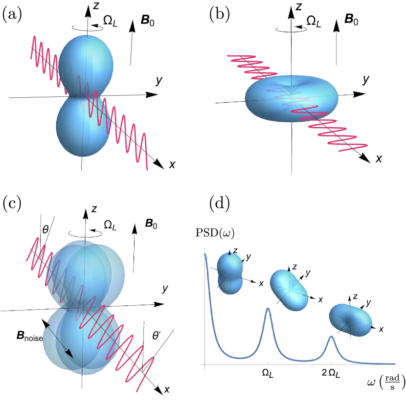
Figure 1: Alignment-based magnetometer: spatial configuration. The light propagates in the direction $x$ in the presence of a strong, static magnetic field $\bm{B}_{0}$, pointing along the $z$-direction. In (a) and (b), angular-momentum probability surfaces of the resulting atomic steady-state are presented, when the atom is pumped by vertically ($\theta=0$) or horizontally ($\theta=\pi/2$) polarised light, respectively. As shown in (c), considering the input light-beam to be polarised at some intermediate angle $0<\theta<\pi/2$, the atomic steady-state generally modifies the polarisation angle of the transmitted light $\theta^{\prime}$. Moreover, in our experiment a stochastic field $\bm{B}_{\mathrm{noise}}$ is applied along the direction of light propagation, and induces white noise that disturbs the atomic state from equilibrium. The so-created randomly tilted state has now three distinct contributions from spherical components ${{\mathcal{T}}}^{(2)}_{0}$, ${{\mathcal{T}}}^{(2)}_{\pm 1}$ and ${{\mathcal{T}}}^{(2)}_{\pm 2}$, whose angular-momentum probability surfaces shown in (d) exhibit periodicity under rotations around $z$ at multiples $0$, $\Omega_{L}$ and $2\Omega_{L}$ of the Larmor (angular) frequency $\Omega_{L}$, respectively. As a result, as depicted in (d), the recorded power spectral density (PSD) of $\theta^{\prime}$-fluctuations should contain three peaks at these particular frequencies with amplitudes dictated by the contribution of each spherical-tensor component.

In Fig. 1 we depict the natural spatial configuration of an alignment-based atomic magnetometer [24], which applies to the implementation considered here. A strong magnetic field $\bm{B}_{0}$, directed along $z$, acts perpendicularly to the direction of light propagation, here chosen to be $x$, with light being linearly polarised at an angle $\theta$ to $z$-axis in the $yz$-plane. Both the field and the light interact with an atom and modify its steady state, otherwise induced solely by the relaxation processes [27]. Although we defer the formal description of the atomic steady-state, let us note for now that its form can be conveniently represented by the angular-momentum probability surface [48, 32] (depicted in blue in Fig. 1). As the surface describes the effective polarisation of the steady state, it indicates the rotation symmetries the state possesses. Its shape strongly depends on the polarisation angle $\theta$ of the input light-beam, e.g., resembling a “peanut” for $\theta=0$ or a “doughnut” for $\theta=\tfrac{\pi}{2}$, see Fig. 1(a) and (b), respectively. Importantly, in our experiment the atom is further disturbed by a stochastic field $\bm{B}_{\mathrm{noise}}$, see Fig. 1(c), that induces white noise along the $x$-direction, whose impact can then be monitored by inspecting the polarisation angle $\theta^{\prime}$ of the transmitted beam, while the atomic state is constantly “kicked out” of equilibrium.

Furthermore, as we carry out the experiment in conditions in which correlations between distinct atoms may be neglected during the sensing process, the dynamics of the whole ensemble is effectively captured by the evolution of a single atom [26]. Due to the effective atomic density being low, the shot noise of the photon-detection process dominates over the atomic projection noise, and the impact of the measurement backaction on the atomic steady-state can be ignored [49]. Moreover, thanks to the presence of a relatively strong magnetic field $\bm{B}_{0}$, given that the experiment is carried out at the room temperature, the mechanism of spin-exchange interactions during atomic collisions is irrelevant [50], in contrast to SERF magnetometers [51], that could in principle induce not only classical correlations but also entanglement between individual atoms [52, 53].

In what follows, we firstly formalise the description of an atomic steady-state in the spherical-tensor representation, in order to then show how such a formalism allows us to compactly model the magnetometer dynamics, as well as predict the behaviour of the detected signal.

II.1 Spherical tensor representation of the atomic steady state

Any density matrix describing an atom of total angular momentum $F$ can always be written in the eigenbasis of the angular-momentum operators $\hat{F}^{2}$ and $\hat{F}_{z}$ as [26]:

$$\rho=\sum_{M,M^{\prime}=-F}^{F}\rho_{MM^{\prime}}^{(F)}\left|F,M\phantom{{}^{\prime}}\right\rangle\!\!\left\langle F,M^{\prime}\right|.$$ (1)

However, it is much more convenient to decompose the density matrix in the basis of spherical tensor operators of rank $\kappa=0,1,\dots,2F$, which transform independently in each $\kappa$-subspace under rotations, and hence magnetic fields, in a well-behaved manner. In particular, we may equivalently write any state (1) as

$$\rho=\sum_{\kappa=0}^{2F}\sum_{q=-\kappa}^{\kappa}m_{\kappa q}{{\mathcal{T}}}^{(\kappa)}_{q},$$ (2)

where the density matrix is now decomposed into a sum of rank-$\kappa$ components, each constituting a sum (over $q$) of, in principle, non-Hermitian tensor operators ${{\mathcal{T}}}^{(\kappa)}_{q}$ multiplied by their corresponding complex coefficients $m_{\kappa q}$. Dealing with an atom of fixed $F$, we drop the explicit $F$-dependence of the terms in Eq. (2). As ${{\mathcal{T}}}^{(\kappa)}_{q}$ form a basis, they formally satisfy $\mathrm{Tr}\!\left\{{{\mathcal{T}}}^{(\kappa)}_{q}({{\mathcal{T}}}^{(\kappa^{\prime})}_{q^{\prime}})^{\dagger}\right\}=\delta_{\kappa\kappa^{\prime}}\delta_{qq^{\prime}}$, while it is convenient to also impose ${{\mathcal{T}}}^{(\kappa){\dagger}}_{q}=(-1)^{q}{{\mathcal{T}}}^{(\kappa)}_{-q}$, so that conditions $m_{\kappa q}=(-1)^{q}m^{*}_{\kappa,-q}$ and $\mathrm{Im}\{m_{\kappa 0}\}=0$ assure then the density matrix (2) to be Hermitian. The $m_{00}=1/\sqrt{2F+1}$ coefficient is fixed by the $\mathrm{Tr}\!\left\{\rho\right\}=1$ condition, while the corresponding ($\kappa=0$) tensor operator, ${{\mathcal{T}}}^{(0)}_{0}=\tfrac{1}{\sqrt{2F+1}}\openone_{2F+1}$, is the only one with a non-zero trace, being invariant under any rotations.

In principle, the atomic steady state may involve more than one $F$-level, e.g. $F=3,4$ in the case of the D1-line transition in caesium. However, if the laser field is tuned to a specific optical transition from a single $F$-level, and there is no coherent coupling between levels of different $F$, one can disregard coherences between these and most generally write the atomic steady state as:

$$\rho=\bigoplus_{F}p_{F}\;\rho^{(F)}.$$ (3)

Moreover, one may then focus on the dynamics of only one particular $\rho^{(F)}$ for the $F$-level actually contributing to the light-atom interaction, with $\rho^{(F)}$ being then decomposable just as in Eq. (2). In what follows, we drop the $(F)$-superscript for simplicity.

As the case of a linearly polarised pump is of our interest, see Fig. 1, from symmetry arguments it follows that, independently of the spin-number $F$, only even-$\kappa$ coefficients are modified when interacting with light [54]. Moreover, as we show later, our model predicts no significant coupling between components of different $\kappa$. On the other hand, it is only the orientation ($\kappa=1$) and alignment ($\kappa=2$) components that can be probed by resorting to electric dipole light-atom interactions [26, 54]. Hence, even though the pump in the experiment is relatively strong, so that $\rho$ in Eq. (2) (for a particular $F$) reads:

$$\rho=\tfrac{1}{2F+1}\openone_{2F+1}+\sum_{q=-2}^{2}m_{2q}{{\mathcal{T}}}^{(2)}_{q}+\sum_{q=-4}^{4}m_{4q}{{\mathcal{T}}}^{(4)}_{q}+\dots,$$ (4)

we may assume that all the information, which is accessible when probing the atomic state $\rho$ with light, is in fact completely determined by the vector containing the alignment coefficients:

$$\textbf{m}=\left(\begin{array}[]{ccccc}m_{2,-2}&m_{2,-1}&m_{2,0}&m_{2,1}&m_{2,2}\end{array}\right)^{\mathrm{T}}.$$ (5)

Furthermore, if the quantisation axis $z$ is chosen along the light polarisation of the pump, $\theta=0$ in Fig. 1(a), by symmetry the atomic steady state must be invariant to any rotations around $z$. Hence, only the (real) coefficient with $q=0$ can acquire some value $m_{2,0}\to m^{\mathrm{ini}}_{20}$, whose maximum (or negative minimum) is theoretically constrained by the positivity of $\rho\geq 0$, but practically by the efficiency of optical pumping being counteracted by relaxation. Considering the light to be linearly polarised at an arbitrary angle to the $xz$-plane, see Fig. 1(c), the steady state can be found by just adequately rotating the above solution for $\theta\!=\!0$ around the light-propagation direction $x$. In particular, the m-vector (5) of the steady state (ss) generated by linearly polarised pump at an angle $\theta$ with respect to the quantisation axis reads, see App. A:

$$\textbf{m}^{\mathrm{ss}}=m^{\mathrm{ini}}_{20}\begin{pmatrix}-\frac{\sqrt{6}}{4}\mathsf{s}_{\theta}^{2}&\mathrm{i}\frac{\sqrt{6}}{4}\mathsf{s}_{2\theta}&1-\frac{3}{2}\mathsf{s}_{\theta}^{2}&\mathrm{i}\frac{\sqrt{6}}{4}\mathsf{s}_{2\theta}&-\frac{\sqrt{6}}{4}\mathsf{s}_{\theta}^{2}\end{pmatrix}^{\mathrm{T}},$$ (6)

where $\mathsf{s}_{\theta}\coloneqq\sin\theta$. However, as the strong static field $\bm{B}_{0}$ leads to fast (Larmor) precession of the atomic state around $z$, see Fig. 1, i.e. with the Larmor (angular) frequency $\Omega_{L}\coloneqq\gamma_{\mathrm{gmr}}|\bm{B}_{0}|$ much greater than the overall relaxation rate, all the multipoles $m_{2,q\neq 0}$ quickly average to zero, so that according to the secular approximation [26] the steady-state vector (6) can then be simplified to

$$\textbf{m}^{\mathrm{ss}}\approx m^{\mathrm{ini}}_{20}\begin{pmatrix}0&0&1\!-\!\frac{3}{2}\sin^{2}\theta&0&0\end{pmatrix}^{\mathrm{T}},$$ (7)

which we assume to be valid throughout this work. The Larmor frequency above is defined using the gyromagnetic ratio $\gamma_{\mathrm{gmr}}\coloneqq g_{F}\mu_{B}/\hbar$ (with units $[\mathrm{rad}\,\mathrm{s}^{-1}\mathrm{T}^{-1}]$), where $g_{F}$ is the Landé g-factor for an atom of total spin $F$ and $\mu_{B}$ is the Bohr magneton.

In order to visualise the symmetries and geometric properties of the steady state (7), we resort to plotting the angular-momentum probability surfaces it yields for $\theta=0$, $\theta=\tfrac{\pi}{2}$ and $0<\theta<\tfrac{\pi}{2}$ in Fig. 1(a), (b) and (c), respectively. In particular, in each case we present a spherical plot of the overlap of the steady state with the state of a maximum angular momentum $\left|F,F\right\rangle_{\bm{n}}$ defined with respect to a given direction $\bm{n}$, which then determines the quantisation axis, i.e.:

$$r(\bm{n})=\,_{\bm{n}}\!\left\langle F,F\right|\rho_{\mathrm{ss}}\left|F,F\right\rangle_{\bm{n}},$$ (8)

where $\rho_{\mathrm{ss}}$ is the steady-state density matrix of the form (4) with the alignment coefficients given by Eq. (7).

In our experiment, as shown in Fig. 1(c), the angular-momentum probability surface of the steady state is constantly perturbed out of equilibrium by the $\bm{B}_{\mathrm{noise}}$-field inducing white noise in the $x$-direction, so that coefficients with $q\neq 0$ in Eq. (7) are no longer zero. As a result, the effective atomic state contains components not only from ${{\mathcal{T}}}^{(2)}_{0}$, but also from ${{\mathcal{T}}}^{(2)}_{\pm 1}$ and ${{\mathcal{T}}}^{(2)}_{\pm 2}$ tensor operators, see Eq. (4), which can be separately visualised by the surfaces depicted in Fig. 1(d). Crucially, as the latter two return to their original state under Larmor precession after being rotated by $2\pi$ and $\pi$, respectively, the measured noisy $\theta^{\prime}$-signal should contain distinct frequency-components at $\Omega_{L}$ and $2\Omega_{L}$. This should be visible when analysing the power spectral density (PSD) of the detected signal, as schematically presented in Fig. 1(d).

II.2 Magnetometer dynamics and measurement

In order to be able to predict the PSD in our experiment, we must move away from just the steady-state description. In particular, we must be able to model the stochastic dynamics of the atoms, so that the auto-correlation function of the detected signal can be computed, whose Fourier transform specifies the PSD.

II.2.1 Atomic stochastic dynamics

Deterministic noisy evolution.

In general, any noisy evolution of the atomic state (1) is described by the Gorini–Kossakowski–Sudarshan–Lindblad equation [55]:

$$\frac{\mathrm{d}\rho}{\mathrm{d}t}=-\frac{\mathrm{i}}{\hbar}[\hat{H},\rho]+\Phi[\rho],$$ (9)

where $\hat{H}$ is the system Hamiltonian, while the map

$$\Phi[\rho]=\sum_{i}\Gamma_{i}(\hat{L}_{i}\rho\hat{L}_{i}^{\dagger}-\frac{1}{2}\{\hat{L}_{i}^{\dagger}\hat{L}_{i},\rho\})$$ (10)

is responsible for the decoherence, with $\hat{L}_{i}$ being the quantum jump (Lindblad) operators and $\Gamma_{i}\geq 0$ the corresponding dissipation rates, which must be non-negative for a Markovian evolution [55].

In the absence of the $\bm{B}_{\mathrm{noise}}$-field, the Hamiltonian incorporates only the interaction of the atom with the static field, i.e. $\hat{H}=\gamma_{\mathrm{gmr}}\bm{B}_{0}\cdot\hat{\bm{F}}=\Omega_{L}\hat{F}_{z}$. However, as the static field introduces anisotropicity in the system, we split the decoherence map as follows:

$$\Phi[\rho]\coloneqq\sum_{\alpha=x,y,z}\Phi_{\alpha}[\rho]+\Phi_{\mathrm{iso}}[\rho],$$ (11)

where

$$\Phi_{\alpha}[\rho] \coloneqq\frac{\Gamma_{\alpha}}{\hbar^{2}}(\hat{F}_{\alpha}\rho\hat{F}_{\alpha}-\frac{1}{2}\{\hat{F}_{\alpha}^{2},\rho\})$$ (12)

can be interpreted as arising from magnetic-field fluctuation in each $\alpha=x,y,z$ direction, whereas:

$$\Phi_{\mathrm{iso}}[\rho] \coloneqq\Gamma_{\mathrm{iso}}\!\left(\sum_{M,M^{\prime}}\!\!\hat{L}_{M,M^{\prime}}\rho\hat{L}_{M,M^{\prime}}^{\dagger}\!-\!\frac{1}{2}\{\hat{L}_{M,M^{\prime}}^{\dagger}\hat{L}_{M,M^{\prime}},\rho\}\right)$$ (13)

with $\hat{L}_{M,M^{\prime}}\coloneqq\frac{1}{\sqrt{2F+1}}\left|F,M\right\rangle\!\!\left\langle F,M^{\prime}\right|$, represents isotropic dissipation that can be equivalently written as

$$\Phi_{\mathrm{iso}}[\rho]=\Lambda-\frac{1}{2}\{\hat{\Gamma},\rho\},$$ (14)

where $\hat{\Gamma}\coloneqq\Gamma_{\mathrm{iso}}\openone_{2F+1}$ and $\Lambda\coloneqq\frac{\Gamma_{\mathrm{iso}}}{2F+1}\,\openone_{2F+1}$ are typically referred to as the re-population and depolarising terms, respectively [32]. Although we assume in our model the rates $\Gamma_{\alpha}$ and $\Gamma_{\mathrm{iso}}$ to be phenomenological and account for various dissipation mechanisms, Eq. (14) can be naturally interpreted as the loss of polarised atoms that then reappear in the beam in a completely unpolarised state.

Impact of the stochastic $\bm{B}_{\mathrm{noise}}$-field.

In our experiment, see Fig. 1(c), stochastic $\bm{B}_{\mathrm{noise}}$-field is applied in the light-propagation direction $x$, which leads to another term in the Hamiltonian $\hat{H}_{\mathrm{noise}}(t)=\gamma_{\mathrm{gmr}}\bm{B}_{\mathrm{noise}}(t)\cdot\hat{\bm{F}}=\gamma_{\mathrm{gmr}}B_{\mathrm{noise}}(t)\hat{F}_{x}$ with

$$B_{\mathrm{noise}}(t)=\frac{\Omega_{\mathrm{noise}}}{\gamma_{\mathrm{gmr}}}\,\xi(t)\;\approx\;\frac{\Omega_{\mathrm{noise}}}{\gamma_{\mathrm{gmr}}}\sqrt{\frac{1}{2\pi f_{\textrm{cutoff}}}}\frac{\mathrm{d}W_{t}}{\mathrm{d}t},$$ (15)

where $\xi(t)$ represents the stochastic process for the noise we generate, see App. C for its further characteristics, which effectively exhibits a constant power spectrum that is cut-off at some frequency $f_{\textrm{cutoff}}$ (in Hz). Now, as we will deal with processes occurring at (angular) frequencies $\omega\ll 2\pi f_{\textrm{cutoff}}$, we approximate such noise in Eq. (15) as being white with the correct rescaling factor—the white noise can be interpreted as the time-derivative, $\frac{\mathrm{d}W}{\mathrm{d}t}$, of the Wiener process, $W_{t}$ [56]. As a result, we can write the (stochastic) time-increment induced by the noise involving the Hamiltonian as

$$\hat{H}_{\mathrm{noise}}(t)\mathrm{d}t=\sqrt{\omega_{\mathrm{noise}}}\,\hat{F}_{x}\,\mathrm{d}W_{t},$$ (16)

where we define $\omega_{\mathrm{noise}}\coloneqq\Omega_{\mathrm{noise}}^{2}/(2\pi f_{\textrm{cutoff}})$ as the effective noise spectral density, while $\mathrm{d}W_{t}\sim\mathcal{N}(0,\mathrm{d}t)$ is then the Wiener increment [56].

In order to correctly include the white noise in the deterministic dynamics (9), we must explicitly compute the time-increment of the density matrix, $\mathrm{d}\rho=\rho(t+\mathrm{d}t)-\rho(t)$, that is now stochastic. By adding the noise contribution to Eq. (9), we define the stochastic map

$$\mathcal{K}(t)[\rho]\coloneqq-\frac{\mathrm{i}}{\hbar}[\hat{H}_{\mathrm{noise}}(t)+\hat{H},\rho]+\Phi[\rho],$$ (17)

which allows us to write for small $\mathrm{d}t$:

$$\rho(t+\mathrm{d}t) =\mathrm{e}^{\mathcal{K}(t)\mathrm{d}t}\left[\rho(t)\right]=\sum_{n=0}^{\infty}\frac{(\mathcal{K}(t)\mathrm{d}t)^{n}[\rho(t)]}{n!}$$

$$=\rho(t)+\mathcal{K}[\rho(t)]\mathrm{d}t+\frac{1}{2}(\mathcal{K}\mathrm{d}t)^{2}[\rho(t)]+O(\mathrm{d}t^{5/2})$$

$$=\rho(t)-\frac{\mathrm{i}}{\hbar}[\hat{H},\rho(t)]\mathrm{d}t+\Phi[\rho(t)]\mathrm{d}t$$

$$-\frac{\mathrm{i}\sqrt{\omega_{\mathrm{noise}}}}{\hbar}[\hat{F}_{x},\rho(t)]\mathrm{d}W_{t}-\frac{\omega_{\mathrm{noise}}}{2\hbar^{2}}[\hat{F}_{x},[\hat{F}_{x},\rho(t)]]\mathrm{d}t$$

$$+O(\mathrm{d}t^{3/2}),$$ (18)

where according to the Itô calculus implying $\mathrm{d}W_{t}^{2}=\mathrm{d}t$ we obtain a dissipative term at the second ($n=2$) order, while all the other terms can be ignored with $\mathrm{d}W_{t}\mathrm{d}t=O(\mathrm{d}t^{3/2})$ within the big-$O$ notation [56].

As a consequence, we obtain the desired stochastic differential equation describing the atomic dynamics as

$$\mathrm{d}\rho =(-\frac{\mathrm{i}}{\hbar}[\hat{H},\rho]+\Phi_{\mathrm{iso}}[\rho])\mathrm{d}t$$

$$+\sum_{\alpha=y,z}\frac{\Gamma_{\alpha}}{\hbar^{2}}(\hat{F}_{\alpha}\rho\hat{F}_{\alpha}-\frac{1}{2}\{\hat{F}_{\alpha}^{2},\rho\})\mathrm{d}t$$

$$+\frac{\Gamma_{x}+\omega_{\mathrm{noise}}}{\hbar^{2}}(\hat{F}_{x}\rho\hat{F}_{x}-\frac{1}{2}\{\hat{F}_{x}^{2},\rho\})\mathrm{d}t$$

$$-\frac{\mathrm{i}\sqrt{\omega_{\mathrm{noise}}}}{\hbar}[\hat{F}_{x},\rho]\mathrm{d}W_{t},$$ (19)

which, apart from the expected term generating random rotations around the $\bm{B}_{\mathrm{noise}}$-field direction, accounts for the fact that (by the fluctuation-dissipation theorem) the white noise must also increase the dissipation rate in the $x$-direction from $\Gamma_{x}$ to $\Gamma_{x}+\omega_{\mathrm{noise}}$.

II.2.2 Spherical-tensor representation

We have argued that when considering the relevant $F$-subspace of the atomic steady state described in Eq. (2), the nature and geometry of light-atom interactions allows us to reduce its form, so that it contains only the alignment component ($\kappa=2$) in Eq. (4). Consistently, as shown in App. A, the evolution determined by Eq. (19) does not couple spherical-tensor components of different rank $\kappa$. Hence, while incorporating optical pumping into the dynamics (19), the evolution of the atomic state must be completely described by the m-vector (5) of, now time-dependent, alignment coefficients, i.e.:

$$\textbf{m}_{t}=\left(\begin{array}[]{ccccc}m_{2,-2}(t)&m_{2,-1}(t)&m_{2,0}(t)&m_{2,1}(t)&m_{2,2}(t)\end{array}\right)^{\mathrm{T}}.$$ (20)

This evolves under the dynamics (19) according to the following stochastic differential equation, see App. A:

$$\mathrm{d}\textbf{m}_{t} =\left(\textbf{A}_{0}+\textbf{A}_{\Phi}+\frac{\textbf{A}_{\mathrm{noise}}^{2}}{2}\right)\textbf{m}_{t}\,\mathrm{d}t+\textbf{A}_{\mathrm{noise}}\,\textbf{m}_{t}\,\mathrm{d}W_{t},$$ (21)

where $\textbf{A}_{0}=-\mathrm{i}\Omega_{L}\textbf{J}^{(2)}_{z}$ and $\textbf{A}_{\mathrm{noise}}=-\mathrm{i}\sqrt{\omega_{\mathrm{noise}}}\textbf{J}^{(2)}_{x}$ are $5\times 5$ matrices that should be associated with the free evolution and stochastic noise, respectively. These are defined with help of the representation of angular momentum operators, $\textbf{J}^{(\kappa)}_{\alpha}$ with $\alpha=x,y,z$, acting on the vector space of alignment—equivalent to ones acting on the state-space of a spin-2 particle, written in the $\{\left|2,-2\right\rangle,\dots,\left|2,2\right\rangle\}$ basis to agree with Eq. (20).

In a similar fashion, the matrix-representation of the dissipative map $\Phi$ in Eq. (11), see App. A, reads

$$\textbf{A}_{\Phi} =-\frac{1}{2}\sum_{\alpha}\Gamma_{\alpha}(\textbf{J}^{(2)}_{\alpha})^{2}-\Gamma_{\mathrm{iso}}\openone_{5}$$

$$\equiv-\textrm{diag}\{\Gamma_{2},\Gamma_{1},\Gamma_{0},\Gamma_{1},\Gamma_{2}\},$$ (22)

which we, however, force above to have a diagonal form postulated in Ref. [27] with three dissipation rates:

$$\bm{\Gamma}\equiv\begin{pmatrix}\Gamma_{0}\\ \Gamma_{1}\\ \Gamma_{2}\\ \end{pmatrix}\coloneqq\begin{pmatrix}6\Gamma_{\perp}+\Gamma_{\mathrm{iso}}\\ \Gamma_{\parallel}+5\Gamma_{\perp}+\Gamma_{\mathrm{iso}}\\ 4\Gamma_{\parallel}+2\Gamma_{\perp}+\Gamma_{\mathrm{iso}}\\ \end{pmatrix}.$$ (23)

Formally, this corresponds to the assumption that in the absence of stochastic noise one should differentiate only between dephasing rates along, $\Gamma_{\parallel}\coloneqq\Gamma_{z}$, and perpendicular to, $\Gamma_{\perp}\coloneqq\Gamma_{x}=\Gamma_{y}$, the static field, while keeping the isotropic depolarisation rate, $\Gamma_{\mathrm{iso}}$, as an independent parameter. The effective rates $\bm{\Gamma}$, see also App. A, are then defined by reparametrising the problem as in Eq. (23).

Finally, in order to include the impact of optical pumping in Eq. (21), we enforce that, in the absence of the noisy magnetic field, the $\textbf{m}_{t}$-vector (20) must converge with time to the steady state described in Sec. II.1. This way, we obtain the desired stochastic dynamical equation for the vector of alignment coefficients as

$$\mathrm{d}\textbf{m}_{t} =(\textbf{A}_{0}+\frac{\textbf{A}_{\mathrm{noise}}^{2}}{2})\textbf{m}_{t}\,\mathrm{d}t+\textbf{A}_{\Phi}(\textbf{m}_{t}-\textbf{m}^{\mathrm{ss}})\,\mathrm{d}t$$

$$+\textbf{A}_{\mathrm{noise}}\textbf{m}_{t}\,\mathrm{d}W_{t},$$ (24)

where the steady state $\textbf{m}^{\mathrm{ss}}$ is given by Eq. (7), being already averaged over the fast (Larmor) precession around $z$ and, hence, satisfying $\textbf{A}_{0}\textbf{m}^{\mathrm{ss}}=\textbf{0}$.

II.2.3 Detected signal

We depict the impact of the Faraday effect in Fig. 1(c), owing to which the angle $\theta$ of the linearly polarised incoming beam is changed to $\theta^{\prime}$ upon leaving the atomic cell. Treating the atomic ensemble as an optically thin sample, the change of the angle, $\Delta\theta\coloneqq\theta^{\prime}-\theta$, obeys then [32]:

$$\Delta\theta\propto\mathrm{i}(\tilde{m}_{2,1}+\tilde{m}_{2,-1}),$$ (25)

with the proportionality constant depending on the optical depth, interaction strength, light power etc.

In the above, $\tilde{m}_{\kappa,q}$ are the alignment coefficients defined with the quantisation axis along the direction of incoming light polarisation, i.e. tilted away by $\theta$ from $z$ in the $yz$-plane, see Fig. 1(c). Hence, Eq. (25) can be re-expressed with help of the $\textbf{m}_{t}$-vector (20) (defined with $z$ being the quantisation axis) by simply rotating $\textbf{m}_{t}$ by an angle $\theta$ around the light-propagation direction $x$, i.e.:

$$\Delta\theta\propto\textbf{h}^{\mathrm{T}}\,\textbf{D}^{(2)}_{\theta}\textbf{m}_{t},$$ (26)

where $\textbf{h}=(0,\mathrm{i},0,\mathrm{i},0)^{\mathrm{T}}$ and $\textbf{D}^{(2)}_{\theta}=D^{(2)}_{m,m^{\prime}}(-\pi/2,\theta,\pi/2)$ is the appropriate Wigner D-matrix, see App. A.

As a result, based on Eq. (26), we may write the detected signal of an alignment-based magnetometer as:

$$S(t) =g_{D}\,\textbf{h}^{\mathrm{T}}\,\textbf{D}^{(2)}_{\theta}\textbf{m}_{t}+\zeta(t)$$

$$=g_{D}\,\tfrac{1}{2}[\sqrt{6}m_{2,0}(t)+m_{2,2}(t)+m_{2,-2}(t)]\sin(2\theta)$$

$$+g_{D}\,\mathrm{i}[m_{2,1}(t)+m_{2,-1}(t)]\cos(2\theta)+\zeta(t),$$ (27)

where $g_{D}$ is the effective proportionality constant, whereas $\zeta(t)$ denotes the detection stochastic noise, which is completely uncorrelated from the magnetic-field noise affecting the atom dynamics in Eq. (24).

It becomes clear from the expression (27) that, as the signal depends on all the alignment coefficients with $q=0,\pm 1,\pm 2$, it must contain components that oscillate at frequencies $0$, $\Omega_{L}$ and $2\Omega_{L}$, respectively. In other words, the signal contains information about different spherical-tensor components of the atomic state, in particular the ones illustrated in Fig. 1(d), each of which should yield a peak in the PSD at the corresponding frequency.

II.3 Experimental setup

Figure 2 shows a schematic of the experimental setup we employ. Linearly polarised light, with a wavelength of 895 nm, is passed through an optical fibre. The light is resonant with the $F=4\rightarrow F^{\prime}=3$ D1 transition of caesium. The light has an electric field amplitude $\bm{E}_{0}$ and passes through a cubic paraffin-coated cell containing caesium atoms, which is placed inside a magnetic shield (Twinleaf MS-1). The cell is $(5\text{mm})^{3}$ and is kept at room temperature ($\sim 18^{\circ}$).

A static magnetic field $\bm{B}_{0}=B_{0}\,\bm{e}_{z}$, with $B_{0}=2.74~{}\mu$T, is applied using the magnetic shield coils. This corresponds to inducing Larmor precession of the atomic spin at a frequency of $f_{L}\approx 10$ kHz. A half-wave plate is placed before the magnetic shield to change the angle of the electric field amplitude of the light, $\bm{E}_{0}$, with respect to the direction of the static magnetic field. Consistently with Fig. 1(c), we denote in Fig. 2 by $\theta$ the angle between the linear polarisation and the $z$-direction in the $yz$-plane, so that, e.g., $\bm{E}_{0}=E_{0}\,\bm{e}_{z}$ for $\theta=0$ and $\bm{E}_{0}=E_{0}\,\bm{e}_{y}$ for $\theta=\pi/2$. In parallel, a noisy magnetic field $\bm{B}_{\mathrm{noise}}(t)=B_{\mathrm{noise}}(t)\,\bm{e}_{x}$ with $B_{\mathrm{noise}}(t)$ being varied in the experiment from $0.132~{}\mathrm{pT_{rms}}$ to $32.92~{}\mathrm{nT_{rms}}$ is applied to the system using a function generator connected to a homemade square Helmholtz coil.

As shown in Fig. 2, after the magnetic shield the polarisation rotation of the transmitted light is measured using a half-wave plate ($\lambda/2$) and a polarising beam splitter (PBS). The half-wave plate is rotated to match exactly the polarisation angle $\theta^{\prime}$ of the transmitted light, see Fig. 1(c), so that it is the deviations from $\theta^{\prime}$ that are then effectively measured via balanced photodection (BPD) . In particular, the difference in the intensity of the outgoing beams from the PBS is tracked using a Thorlabs balanced photodetector (PDB210A/M). The output photocurrent is recorded in real time using a data acquisition card. Further technical details on the magnetometer can also be found in Ref. [25].

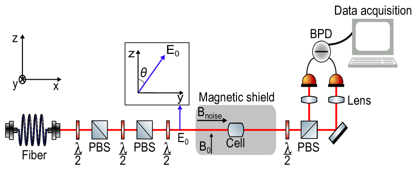
Figure 2: Alignment-based magnetometer: experimental setup. The laser light propagates along the $x$-direction, while the angle $\theta$ of its linear polarisation can be adjusted by rotating half-wave plates ($\lambda/2$) before it enters the magnetic shield (marked in grey). Within the shield, the light simultaneously pumps and probes the atomic ensemble of caesium atoms contained within a paraffin-coated cell (Cell). The atoms are subject to (strong) static and (relatively weak) noisy magnetic fields: $\bm{B}_{0}$ applied in the $z$-, and $\bm{B}_{\mathrm{noise}}$ applied in the $x$-direction, respectively. Due to the Faraday effect, the polarisation of the light exhibits rotation, which is then measured by passing the output beam through a polarising beam splitter (PBS) and performing balanced photodetection (BPD).

Importantly, as our experiment matches the spatial configuration of an alignment-based magnetometer described in previous sections, we can interpret the measured photocurrent of the BPD exactly as $\delta S(t)\coloneqq S(t)-\left\langle S(t)\right\rangle$, i.e. as deviations from the mean value of the detected signal stated in Eq. (27). The effective proportionality constant $g_{D}$ in Eq. (27), which relates the instantaneous atomic state to the photocurrent signal, is then dictated by a number of experimental conditions including: the light power (1 $\mu W$), pumping efficiency, size of the vapour cell ((5 mm)³), as well as the temperature (room temperature, $\sim 18^{\circ}$). On the other hand, the detection noise, $\zeta(t)$ in Eq. (27), should be attributed to photon shot-noise and electronic jitter arising solely due to the photo-detection process that effectively leads to a background noise—within the measured PSD a DC offset is observed independently whether the light beam interacts with the atoms or not. This results in a noise floor that depends on the frequency, partially due to the 1/f noise. This will be taken into account when interpreting the data in Sec. III.2 below.

III Spin noise spectroscopy

Denoting the Fourier transform of any signal, here the measured current of the balanced photodetector $\delta S(t)$, over a finite-time interval $[0,T]$ as:

$$\delta S(\omega)=\frac{1}{\sqrt{T}}\int_{0}^{T}\mathrm{d}t\mathrm{e}^{-\mathrm{i}\omega t}\delta S(t),$$ (28)

its power spectral density (PSD) is defined as [33]:

$$\mathrm{PSD}(\omega)\coloneqq\left\langle|\delta S(\omega)|^{2}\right\rangle,$$ (29)

where by $\left\langle\dots\right\rangle$ we denote throughout the article an average over stochastic trajectories.

Importantly, provided that $\delta S(t)$ is stationary and ergodic, which can be assured by letting $T\gg\tau_{\mathrm{coh}}$ in Eq. (28) where $\tau_{\mathrm{coh}}$ is some effective coherence time of the noisy system under study, we may rewrite the power spectrum according to the Wiener-Khinchin theorem as [33]:

$$\mathrm{PSD}(\omega)\;\underset{\textrm{ss}}{=}\;2\int_{0}^{\infty}\mathrm{d}t\cos(\omega t)\left\langle S(t),S(0)\right\rangle,$$ (30)

where by “ss”, as before, we emphasise the above to hold in the steady state. Crucially, Eq. (30) is now expressed in terms of the auto-covariance function of the detected signal, $S(t)$ specified in Eq. (27), i.e. $\left\langle S(t_{1}),S(t_{2})\right\rangle\coloneqq\left\langle S(t_{1})S(t_{2})\right\rangle-\left\langle S(t_{1})\right\rangle\left\langle S(t_{2})\right\rangle$ .

Substituting explicitly the form of the detected signal (27) into Eq. (30), we obtain the form of the PSD applicable to our problem as

$$\mathrm{PSD}(\omega)=g_{D}^{2}\,\textbf{h}^{\mathrm{T}}\,\textbf{D}^{(2)}_{\theta}\mathbf{\Xi}(\omega)\textbf{D}^{(2)\mathrm{T}}_{\theta}\textbf{h}+\left\langle|\zeta(\omega)|^{2}\right\rangle,$$ (31)

where the (5x5) matrix $\mathbf{\Xi}(\omega)$ is defined as:

$$\Xi_{pq}(\omega)\coloneqq 2\int_{0}^{\infty}\mathrm{d}t\cos(\omega t)\langle m_{2,p}(t),m_{2,q}(0)\rangle,$$ (32)

with $p,q=-2,..,2$ specifying the coefficients of the $\textbf{m}_{t}$-vector (20) evaluated in the steady state. As expected, the detection noise $\zeta(\omega)$, being uncorrelated from any other noise sources, leads to just a noise floor in Eq. (29).

III.1 Theoretical predictions

The alignment dynamics derived in Eq. (24) constitutes an example of a stochastic inhomogeneous evolution [56], for which one can explicitly determine the form of the $\bm{\Xi}(\omega)$-matrix appearing in the PSD (29), see App. B, i.e.:

$$\bm{\Xi}(\omega)=(\textbf{A}_{\mathrm{det}}+\mathrm{i}\omega)^{-1}\textbf{A}_{\mathrm{noise}}\,\bm{\sigma}\,(\textbf{A}_{\mathrm{noise}})^{\mathrm{T}}(\textbf{A}_{\mathrm{det}}^{\mathrm{T}}-\mathrm{i}\omega)^{-1},$$ (33)

where by $\textbf{A}_{\mathrm{det}}\coloneqq\textbf{A}_{0}+\textbf{A}_{\Phi}+\tfrac{1}{2}\textbf{A}_{\mathrm{noise}}^{2}$ we denote for short the overall matrix responsible in Eq. (21) for the deterministic evolution. The (covariance) matrix $\bm{\sigma}$ above is then, see App. B, the solution of the linear equation:

$$\textbf{A}_{\mathrm{det}}\bm{\sigma}+\bm{\sigma}\textbf{A}_{\mathrm{det}}^{\mathrm{T}}+\textbf{A}_{\mathrm{noise}}\,\bm{\sigma}\,(\textbf{A}_{\mathrm{noise}})^{\mathrm{T}}$$

$$=\textbf{A}_{\Phi}\textbf{m}^{\mathrm{ss}}(\textbf{m}^{{\mathrm{ss}}})^{\mathrm{T}}{\textbf{A}_{\Phi}}^{\mathrm{T}}(\textbf{A}_{\mathrm{det}}^{\mathrm{T}})^{-1}$$

$$\qquad+(\textbf{A}_{\mathrm{det}})^{-1}\textbf{A}_{\Phi}\textbf{m}^{\mathrm{ss}}(\textbf{m}^{{\mathrm{ss}}})^{\mathrm{T}}{\textbf{A}_{\Phi}}^{\mathrm{T}},$$ (34)

which can always be solved fast numerically, given $\textbf{A}_{0}$, $\textbf{A}_{\mathrm{noise}}$, $\textbf{A}_{\mathrm{\Phi}}$ and $\textbf{m}^{\mathrm{ss}}$.

However, independently of the particular form of $\bm{\sigma}$, one can show that the PSD (31) for our problem, see App. B.1, must correspond to a sum of absorptive and dispersive Lorentzian functions:

$$\mathrm{PSD}(\omega)= \sum_{j=-2,..,2}\frac{p_{|j|}^{a}\gamma_{|j|}^{2}}{(\omega-\omega_{j})^{2}+\gamma_{|j|}^{2}}$$ (35)

$$+\sum_{j=\pm 1,\pm 2}\frac{\pm p_{|j|}^{d}\gamma_{|j|}(\omega-\omega_{j})}{(\omega-\omega_{j})^{2}+\gamma_{|j|}^{2}}+\left\langle|\zeta(\omega)|^{2}\right\rangle,$$

whose central frequencies, $\omega_{j}$, read

$$\omega_{0} =0,\quad\omega_{1}=-\omega_{-1}=\sqrt{\Omega_{L}^{2}-\frac{9}{16}\omega_{\mathrm{noise}}^{2}},$$

$$\omega_{2} =-\omega_{-2}\approx 2\Omega_{L}-\frac{3}{16}\frac{\omega_{\mathrm{noise}}^{2}}{\Omega_{L}},$$ (36)

and, as expected, up to negligible corrections $O(\omega_{\mathrm{noise}}^{2}/\Omega_{L})$ correspond to multiples of the Larmor frequency: $0$, $\Omega_{L}$ and $2\Omega_{L}$. Whereas, the line widths (half-widths at half maxima), $\gamma_{|j|}$, take the form

$$\gamma_{0} \approx\Gamma_{0}+\frac{3}{2}\omega_{\mathrm{noise}},\quad\gamma_{1}=\Gamma_{1}+\frac{5}{4}\omega_{\mathrm{noise}},$$

$$\gamma_{2} \approx\Gamma_{2}+\frac{1}{2}\omega_{\mathrm{noise}}.$$ (37)

All $\omega_{j}$ and $\gamma_{|j|}$ stated in Eqs. (36) and (37), respectively, can be determined analytically, however, we already simplified their forms above for $\omega_{\pm 2}$, $\gamma_{0}$ and $\gamma_{2}$, which are given $\forall_{j}:\;\Omega_{L}\gg\Gamma_{|j|}$ and $\Omega_{L}\gg\omega_{\mathrm{noise}}$.

In particular, these assumptions are guaranteed in our experiment, in which the static field $B_{0}$ is always much stronger than the noisy field $B_{\mathrm{noise}}$ and yields the Larmor frequency $\Omega_{L}$ much greater than any of the dissipation rates forming $\bm{\Gamma}$ in Eq. (23). Moreover, under these assumptions we can compute analytically also the peak heights, $p_{|j|}^{a/d}$, which in the absorptive case then read

$$p^{a}_{0}=C\,\frac{27}{16}\;\omega_{\mathrm{noise}}^{2}\;\frac{\Gamma_{0}^{2}(2\Gamma_{2}+\omega_{\mathrm{noise}})}{(2\Gamma_{0}+3\omega_{\mathrm{noise}})^{2}G(\omega_{\mathrm{noise}},\bm{\Gamma})}\;h(\theta),$$ (38a)

$$p^{a}_{1}=C\,\frac{3}{4}\;\omega_{\mathrm{noise}}\;\frac{\Gamma_{0}^{2}(2\Gamma_{2}+\omega_{\mathrm{noise}})}{(4\Gamma_{1}+5\omega_{\mathrm{noise}})\,G(\omega_{\mathrm{noise}},\bm{\Gamma})}\;g(\theta),$$ (38b)

$$p^{a}_{2}=C\,\frac{3}{32}\;\omega_{\mathrm{noise}}^{2}\;\frac{\Gamma_{0}^{2}}{(2\Gamma_{2}+\omega_{\mathrm{noise}})\,G(\omega_{\mathrm{noise}},\bm{\Gamma})}\;h(\theta),$$ (38c)

with

$$G(\omega_{\mathrm{noise}},\bm{\Gamma})\coloneqq(2\Gamma_{0}+3\omega_{\mathrm{noise}})\{3\omega_{\mathrm{noise}}^{2}[\Gamma_{0}+2(\Gamma_{1}+\Gamma_{2})]$$

$$\;\;+2\omega_{\mathrm{noise}}(2\Gamma_{0}\Gamma_{1}+5\Gamma_{0}\Gamma_{1}+6\Gamma_{1}\Gamma_{2})+8\Gamma_{0}\Gamma_{1}\Gamma_{2}\},$$ (39)

and the proportionality constant $C\coloneqq g_{D}^{2}(m^{\mathrm{ini}}_{20})^{4}$.

The dispersive equivalents of expressions (38) can also be determined analytically (given $\forall_{j}:\;\Omega_{L}\gg\Gamma_{|j|}$ and $\Omega_{L}\gg\omega_{\mathrm{noise}}$) and can be found in App. C. However, see App. C.1, these are irrelevant upon substituting the parameters applicable to our experiment. Hence, we ignore their contribution to the PSD (35) from now on.

Although Eqs. (38) allow us to predict the dependence of the peak heights for all values of noise intensity $\omega_{\mathrm{noise}}$, it directly follows that for low noise-strengths they obey $p_{0}^{a}~{}\propto~{}\omega_{\mathrm{noise}}^{2}$, $p_{1}^{a}\propto\omega_{\mathrm{noise}}$, and $p_{2}^{a}\propto\omega_{\mathrm{noise}}^{2}$. Furthermore, their angular dependence factorises and is given by

$$h(\theta)\coloneqq[2\sin(2\theta)+3\sin(4\theta)]^{2}$$ (40)

for $p_{0}^{a}$ and $p_{2}^{a}$, whereas for $p_{1}^{a}$ it reads

$$g(\theta)\coloneqq[3+2\cos(2\theta)+3\cos(4\theta)]^{2}.$$ (41)

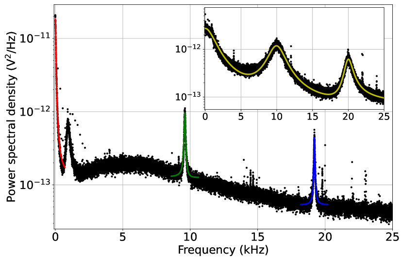
Figure 3: Power spectral density (PSD) measured in the experiment against the theoretical fits predicted by Eq. (35). The signal was recorded over 100 time traces, each of 1 second duration. Within the main plot, relatively low-noise spectral density of $f_{\mathrm{noise}}=0.26$ Hz is chosen, corresponding to 140 mV_rms (the input polarisation angle is set to $\theta=40^{\circ}$). The so-obtained PSD is then fitted with help of separate Lorentzian functions centred around the three peaks at $f=0$, $f_{L}$ and $2f_{L}$ (red, green and blue curves, respectively). In contrast, the inset shows the PSD for high-noise spectral density $f_{\mathrm{noise}}=120$ Hz, corresponding to 3 V_rms (with the input polarisation angle set now to $\theta=25^{\circ}$). In such a case, a single fit-function for all three peaks must be used (yellow curve).

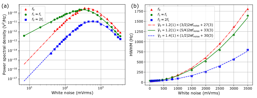
Figure 4: Amplitudes (a) and line-widths (b) of the PSD peaks as a function of the white-noise strength, which is varied from 7 $\mathrm{mV_{rms}}$ to 3500 $\mathrm{mV_{rms}}$ with the light polarisation angle fixed to $\theta=25^{\circ}$. For every white-noise value $V_{\mathrm{noise}}$, amplitudes and line-widths are determined for each of the three relevant (absorptive) peaks in the PSD via the fitting procedure described in Fig. 3. Using the same colouring as in the main plot of Fig. 3, the theoretical predictions are shown for each peak at $0$ (red, dot-dashed), $\approx f_{L}$ (green, solid) and $\approx 2f_{L}$ (blue, dashed) frequency. (a) All three peak amplitudes $\widetilde{p}_{j}^{a}$ clearly follow the theoretical predictions of Eq. (38), which we fit by tuning only the overall proportionality constants ($C_{j}$ for each $j$, see main text) while using the values of dissipation rates $\widetilde{\bm{\Gamma}}$ determined from the line-width data. (b) As predicted by Eq. (37), the line-widths increase linearly with $f_{\mathrm{noise}}$($=cV_{\mathrm{noise}}^{2}$) with proportionality constants agreeing almost exactly for each peak. The line-widths at $V_{\mathrm{noise}}=0$ provide then the corresponding dissipation rates $\widetilde{\bm{\Gamma}}$ (in Hz): $\widetilde{\Gamma}_{0}=27(3)$, $\widetilde{\Gamma}_{1}=33(3)$ and $\widetilde{\Gamma}_{2}=30(3)$.

III.2 Measured noise spectra

In order to validate the theoretical model outlined above, we vary the noisy magnetic field in the table-top alignment-based magnetometer described in Sec. II.3. For the purpose of experiment, we define the noise spectral density in Hz, i.e. $f_{\mathrm{noise}}$ such that $\omega_{\mathrm{noise}}=2\pi f_{\mathrm{noise}}$. As we apply a known voltage through the coil, it is convenient to further write $f_{\mathrm{noise}}=c\,V_{\mathrm{noise}}^{2}$, where $V_{\mathrm{noise}}^{2}$ has now units of $\mathrm{mV_{rms}}$ and the proportionality constant $c$ can be explicitly determined for our setup, see App. D.

In order to measure the PSD (29) of our device, we record one hundred one-second data sets, for each of which the Fourier transform is then computed before averaging. The main plot of Fig. 3 shows an exemplary PSD obtained for the input polarisation angle being set to $\theta=40^{\circ}$, and the applied noise spectral density to $V_{\mathrm{noise}}=140$ mV_rms (corresponding to $f_{\mathrm{noise}}=0.26$ Hz). It is clear that the PSD has peaks at approximately $0$, $f_{L}$ and $2f_{L}$ frequencies with $\Omega_{L}=2\pi f_{L}$, as predicted.

For such a low strength of white noise the three peaks are clearly separated and effectively experience detection noise (and $1/f$-noise) of different strengths. Hence, we fit the absorptive Lorentzian functions appearing in Eq. (35) to each of them individually, i.e. we fit independently around each peak with $j=0,1,2$ the profile:

$$\mathrm{PSD}_{j}(f)=\frac{\widetilde{p}_{j}^{a}\widetilde{\gamma}_{j}^{2}}{(f-f_{j})^{2}+\widetilde{\gamma}_{j}^{2}}+\left\langle|\widetilde{\zeta}_{j}(f)|^{2}\right\rangle,$$ (42)

where the central frequencies $f_{j}\approx jf_{L}$ (with $f_{0}=0$ imposed) and the line widths $\widetilde{\gamma}_{j}=\gamma_{j}/2\pi$ are now expressed in Hz, while both the peak amplitude and noise floor, $\widetilde{p}_{j}$ and $\left\langle|\widetilde{\zeta}_{j}(f)|^{2}\right\rangle$ respectively, have units of $\mathrm{V}^{2}/\mathrm{Hz}$.

$j$	$f_{j}$	$\widetilde{\gamma}_{j}$	$\widetilde{p}_{j}^{a}$	$\left\langle|\widetilde{\zeta}(f)|^{2}\right\rangle$
	(Hz)	(Hz)	(V2/Hz)	(V2/Hz)
$0$	$0$	$34.3(3)$	$9.15(5)\times 10^{-12}$	$6.5(8)\times 10^{-14}$
$1$	$9603.1(3)$	$48.9(4)$	$4.17(2)\times 10^{-13}$	$6.35(4)\times 10^{-14}$
$2$	$19208.0(3)$	$37.9(4)$	$1.97(1)\times 10^{-13}$	$2.67(2)\times 10^{-14}$

Table 1: Best-fit parameters in the low-noise regime. Each of the three individual peaks in the main plot of Fig. 3 was fitted independently to the Lorentzian profile (42) to obtain the fit-parameters presented. For this data set, the light polarisation angle was set to $\theta=40^{\circ}$ and the strength of applied noise was set to 140 mV_rms such that $f_{\mathrm{noise}}=0.26$ Hz.

The corresponding fit parameters obtained for each of the three peaks are listed in Table 1. Due to a clear separation of the peaks, the noise floor varies between them—it takes the value of approximately $6.5\times 10^{-14}$ V²/Hz for the peaks centred at $f_{0}=0$ and $f_{1}\approx f_{L}$, while it reads about $2.7\times 10^{-14}$ V²/Hz for the peak at $f_{2}\approx 2f_{L}$.

In contrast, when dealing with high strengths of white noise ($V_{\mathrm{noise}}\geq 1~{}\mathrm{V_{rms}}$), the three peaks strongly overlap within the PSD, as shown explicitly for $V_{\mathrm{noise}}=3~{}\mathrm{V_{rms}}$ within the inset of Fig. 3. As predicted by the theory, this is due to an apparent increase of the peak line-widths. Moreover, as the peak amplitudes are then at least an order of magnitude above the noise floor, the latter may be assumed to be frequency-independent. As a consequence, it is then correct to fit a single function to the whole PSD, i.e. the complete absorptive part of Eq. (35).

In what follows, we verify in more detail the expressions (38) for the peak amplitudes by studying explicitly their dependence on the noise spectral density, $f_{\mathrm{noise}}$, and the light polarisation angle, $\theta$.

III.2.1 Varying the noise spectral density

Figures 4(a) and 4(b) show the variation of the amplitude and line-width, respectively, for each of the Lorentzian peaks fitted around $f=0$, $f_{L}$ and $2f_{L}$, as a function of the white-noise strength $V_{\mathrm{noise}}$ in $\mathrm{mV^{2}_{rms}}$ units (same colouring as in the main plot of Fig. 3). The data was collected with a fixed, $\theta=25^{\circ}$, polarisation angle of the input beam. As described above, for low white-noise strengths, $V_{\mathrm{noise}}<1~{}\mathrm{V_{rms}}$, the fitting procedure was done while treating each of the peaks separately, whereas for higher values of noise a single fitting-function was used.

Crucially, the experimental results are consistent with the theory, in particular, the amplitudes of the three (absorptive) peaks follow the functional dependences predicted by Eq. (38), with e.g. quadratic and linear dependences: $\widetilde{p}_{0}^{a}~{}\propto~{}f_{\mathrm{noise}}^{2}$, $\widetilde{p}_{1}^{a}\propto f_{\mathrm{noise}}$, and $\widetilde{p}_{2}^{a}\propto f_{\mathrm{noise}}^{2}$ with $f_{\mathrm{noise}}\propto V^{2}_{\mathrm{noise}}$ (now in Hz); easily verifiable from Fig. 4(a) in the low white-noise regime. On the other hand, the corresponding line-widths depicted in Fig. 4(b) follow quadratic dependences in $V_{\mathrm{noise}}$ predicted by Eq. (37), which allows us to determine the effective dissipation rates (23) that take values $\widetilde{\Gamma}_{0}=27(3)$ Hz, $\widetilde{\Gamma}_{1}=33(3)$ Hz and $\widetilde{\Gamma}_{2}=30(3)$ Hz for $f=0$, $f_{L}$ and $2f_{L}$ peaks, respectively. Moreover, in both cases we obtain the proportionality constant in $f_{\mathrm{noise}}=cV^{2}_{\mathrm{noise}}$ to be best approximated by $c=1.33(2)\times 10^{-5}~{}\mathrm{Hz/mV^{2}_{rms}}$, which is in agreement with the value obtained independently via the calibration described in App. D. Although the theory does not allow us to predict the proportionality constant $C$ shared by all the peak amplitudes in Eq. (38), we determine its value separately for each $\widetilde{p}^{a}_{0}$, $\widetilde{p}^{a}_{1}$ and $\widetilde{p}^{a}_{2}$ in Fig. 4(a). We obtain $C_{0}=2.97(7)\times 10^{-6}~{}\mathrm{V}^{2}$, $C_{1}=1.88(4)\times 10^{-6}~{}\mathrm{V}^{2}$ and $C_{3}=1.18(3)\times 10^{-6}~{}\mathrm{V}^{2}$, respectively, which consistently are of the same order.

Last but not least, let us comment that our theoretical model is incapable of predicting shifts in the central frequencies of the peaks, as it would force $f_{j}=j\,f_{L}$ in Eq. (42) with the corrections to $\omega_{j}=2\pi f_{j}$ predicted by Eq. (36) not only being negative, but also appearing at a negligible $O(\omega_{\mathrm{noise}}^{2}/\Omega_{L}=f_{\mathrm{noise}}^{2}/f_{L})$ order—ranging between $10^{-5}$ Hz and $1$ Hz for parameters of our experiment. Nonetheless, we investigate explicitly the shifts of central frequencies $f_{1}\approx f_{L}$ and $f_{2}\approx 2f_{L}$ with the white-noise strengths in Fig. 5. Surprisingly, these increase linearly with $f_{\mathrm{noise}}$ (quadratically with $V_{\mathrm{noise}}$) reaching up to $\Delta f_{j}\coloneqq f_{j}-jf_{L}\approx 1$ kHz for the strongest white-noise applied. Although the stochastic dynamics (24) does not anticipate such a phenomenon, it can be incorporated phenomenologically by letting the “effective” Larmor frequencies depend on the white-noise strength, so that assuming the shifts to depend linearly on the noise density we obtain $\Delta f_{j}=\chi_{j}f_{\mathrm{noise}}$ with $\chi_{1}=4.0$ and $\chi_{2}=6.2$ for the data of Fig. 5.

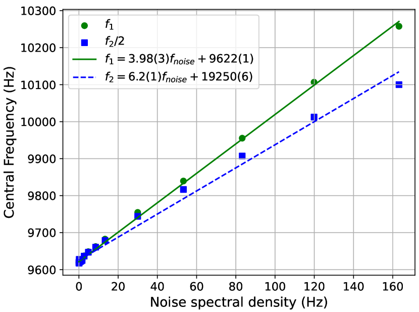
Figure 5: Central frequency of the PSD peaks as a function of the noise spectral density ($f_{\mathrm{noise}}$), which is varied from 7 $\mathrm{mV_{rms}}$ to 3500 $\mathrm{mV_{rms}}$ with the light polarisation angle being fixed to $\theta=25^{\circ}$. Although the shifts observed are not predicted by our theoretical model, we fit the linear (quadratic) dependence of $\Delta f_{j}\coloneqq f_{j}-jf_{l}$ on $f_{\mathrm{noise}}$ ($V_{\mathrm{noise}}$) to obtain phenomenological shift dependencies $\Delta f_{j}=\chi_{j}f_{\mathrm{noise}}$ with $\chi_{1}=4.0$ and $\chi_{2}=6.2$ for the peaks centred around the frequencies $f_{L}$ ($j=1$, green solid) and $2f_{L}$ ($j=2$, blue dashed).

III.2.2 Varying the light polarisation angle

Finally, as the angular dependence of the peak amplitudes (38) separates from all other parameters in the form of functions $h[\theta]$ and $g[\theta]$ stated in Eqs. (40) and (41), we verify this explicitly in the low white-noise regime with $V_{\mathrm{noise}}=$140 $\mathrm{mV_{rms}}$ (each peak fitted separately according to Eq. (42)), by varying the polarisation angle of the incoming light from $\theta=-20^{\circ}$ to $\theta=120^{\circ}$. The results are presented in Fig. 6 with measurements reproducing almost exactly the predicted angular behaviours. As the line-widths of the peaks do not vary significantly when varying $\theta$ (data not shown), we may use the values $\widetilde{\gamma}_{j}$ determined for this low value of noise in Fig. 4(a) and compute separately the exact proportionality constants for each $\widetilde{p}^{a}_{j}$ such that the functions $h[\theta]$ and $g[\theta]$ are most accurately reproduced. In this way, while accounting also for a common angular offset $\theta\to\theta+\delta\theta$ with $\delta\theta=0.77(7)^{\circ}$ in our setup, we obtain $C_{0}=3.1(5)\times 10^{-6}$ V, $C_{1}=2.0(1)\times 10^{-6}$ V and $C_{2}=1.3(4)\times 10^{-6}$ V, which are consistently of similar magnitude and almost the same as the ones determined above when varying the white-noise strength.

Figure 6: Amplitudes of the PSD peaks as a function of the light polarisation angle, which is varied from $\theta=-20^{\circ}$ to $\theta=120^{\circ}$ with the white-noise strength set to $V_{\mathrm{noise}}=140~{}\mathrm{mV_{rms}}$. The fits predicted theoretically by Eq. (38), in particular, the angular dependences $h[\theta]$ and $g[\theta]$ stated in Eqs. (40) and (41), are shown as solid curves for the peaks centred around frequencies $0$ (red), $f_{L}$ (green) and $2f_{L}$ (blue).

IV Conclusions

We prepare a detailed dynamical model allowing us to predict spin-noise spectra of an alignment-based magnetometer, which we then verify experimentally. Its applicability relies on the presence of the excess white-noise being applied along the propagation direction of the light beam that is used to both pump and probe the atomic ensemble, which is perpendicular to the direction of the strong magnetic field responsible for Larmor precession.

On one hand, the added noise amplifies the Larmor-induced peaks to be clearly visible within the power spectral density above the level of detection noise, so that thanks to our model the device can be used as a scalar magnetometer to track fast changes (beyond the magnetometer bandwidth [46]) of the strong magnetic field in real time [59, 60]. On the other, the induced noise can be used to naturally perform sensing tasks in the so-called covert manner [61], i.e. so that an adversary having access to the output of the magnetometer would not be able to recover the signal without possessing the pre-calibrated dynamical model that we propose. In this sense, we expect our model to be useful also for tracking time-varying signals encoded in oscillating RF-fields (amplitude/phase) directed perpendicularly to both the scalar field and the added noise.

It would be interesting to generalise our model to a device that operates at the quantum limit [35, 36, 37], i.e. with detection noise being small enough, so that the predicted peaks in the spectrum arise without the need to artificially amplify them by applying the excess classical noise. Moreover, similarly to orientation-based magnetometers [38, 62, 63], maybe such model could be also capable to incorporate the effect of pumping and probing the ensemble with squeezed light, so the detection noise can be even further reduced. We leave such open questions for the future.

Appendix A Evolution in the basis of spherical tensor operators

The evolution of the atomic ensemble without the effect of pumping, described by Eq. (19), is written in terms of the density matrix (1). In this appendix we show how to write it in terms of the vector of all spherical tensor components $\textbf{m}_{t}^{\mathrm{full}}$. In particular, since the right-hand side of the equation is linear in terms of $\rho$, we would like to find specific linear operators that act on $\textbf{m}_{t}^{\mathrm{full}}$ that correspond to specific operations performed on $\rho$, and enable us to write the dynamical equation in the form of (21). We also show that, since the resulting operators do not couple spherical tensor components of different rank, we only need rank-2 component for a full description of the problem under consideration.

A.1 Rotations induced by magnetic fields

Spherical-tensor operators, ${{\mathcal{T}}}^{(\kappa)}_{q}$, form a convenient basis for density matrices of a system with fixed angular momentum $F$:

$${\rho}=\sum_{\kappa=0}^{2F}\sum_{q=-\kappa}^{\kappa}m_{\kappa q}{{\mathcal{T}}}^{(\kappa)}_{q},$$ (43)

with a scalar product $\mathrm{Tr}\Big{[}{{{\mathcal{T}}}^{(\kappa)}_{q}}^{\dagger}{{\mathcal{T}}}^{(\kappa^{\prime})}_{q^{\prime}}\Big{]}=\delta_{\kappa\kappa^{\prime}}\delta_{qq^{\prime}}$, and with well-defined behaviour under rotations generated by the angular-momentum operators, i.e. a vector $\hat{\bm{F}}:=(\hat{F}_{x},\hat{F}_{y},\hat{F}_{z})^{T}$. In particular, any $SO(3)$ rotation can be parameterised either by the axis (represented by a normalised vector $\bm{n}$), and angle of rotation $\varphi$:

$$\hat{\mathcal{R}}(\bm{n},\varphi)=\mathrm{e}^{-\mathrm{i}\varphi\bm{n}\cdot\hat{\bm{F}}},$$ (44)

or by the three Euler angles $\phi$, $\theta$, $\psi$ that correspond to subsequent rotations about the $z$-, $y$- and again the $z$-axes, respectively:

$$\hat{\mathcal{R}}(\psi,\theta,\phi)=\mathrm{e}^{-\mathrm{i}\psi\hat{F}_{z}}\mathrm{e}^{-\mathrm{i}\theta\hat{F}_{y}}\mathrm{e}^{-\mathrm{i}\phi\hat{F}_{z}}.$$ (45)

We now use the operator above to define the Wigner D-matrix:

$$D^{(F)}_{M,M^{\prime}}(\psi,\theta,\phi):=\langle F,M|\hat{\mathcal{R}}(\psi,\theta,\phi)|F,M^{\prime}\rangle.$$ (46)

The spherical tensor operators behave analogously to angular momentum eigenstates under rotations if we treat the rank $\kappa$ as the total angular momentum, and the index $q$ as the projection on the $z$ axis:

$$\hat{\mathcal{R}}(\psi,\theta,\phi){{\mathcal{T}}}^{(\kappa)}_{q^{\prime}}\hat{\mathcal{R}}(\psi,\theta,\phi)^{\dagger}=\sum_{q=-\kappa}^{\kappa}D^{(\kappa)}_{q,q^{\prime}}(\psi,\theta,\phi){{\mathcal{T}}}^{(\kappa)}_{q}.$$ (47)

This means that for the spherical tensor component vector $\textbf{m}_{t}^{(\kappa)}$ composed of $m_{\kappa,q}(t)$ coefficients ($q=-\kappa,...,\kappa$), the rotation generators are $\textbf{J}^{(\kappa)}_{x}$, $\textbf{J}^{(\kappa)}_{y}$ and $\textbf{J}^{(\kappa)}_{z}$, which are the matrix representations of angular momentum operators cut to the subspace of total angular momentum $\kappa$.

This simplifies the study of dynamics of $\rho$ under rotations, but also facilitates the description of light-atom interactions. Whenever one considers dipole-type interactions, which correspond to multiplying two (dipole) vectors, spherical-tensor components with $\kappa\leq 2$ describing the atom are sufficient to find the output light state. [26, 54].

We use these properties of the spherical tensor to find the expressions for the evolution of the atomic state described by Eq. (19) in the spherical tensor basis. Since the Hamiltonian resulting from the magnetic field generates the rotation of the atomic state about the magnetic field vector $\bm{B}$:

$$\frac{\mathrm{d}\rho}{\mathrm{d}t}=-\mathrm{i}[\gamma_{\mathrm{gmr}}\bm{B}\cdot\hat{\bm{F}},\rho],$$ (48)

the evolution in the spherical tensor basis will also be driven by respective rotation generators:

$$\frac{\mathrm{d}\textbf{m}_{t}^{(\kappa)}}{\mathrm{d}t}=-\mathrm{i}\gamma_{\mathrm{gmr}}(\bm{B}\cdot\bm{J}^{(\kappa)})\textbf{m}_{t}^{(\kappa)},$$ (49)

where $\bm{J}^{(\kappa)}=\left(\textbf{J}^{(\kappa)}_{x},\textbf{J}^{(\kappa)}_{y},\textbf{J}^{(\kappa)}_{z}\right)^{\mathrm{T}}$.

This can be directly shown using the commutation relations for the spherical tensor operators and the angular momentum operators:

$$[\hat{F}_{z},{{\mathcal{T}}}^{(\kappa)}_{q}] =\hbar q{{\mathcal{T}}}^{(\kappa)}_{q},$$ (50)

$$[\hat{F}_{\pm},{{\mathcal{T}}}^{(\kappa)}_{q}] =\hbar\sqrt{\kappa(\kappa+1)-q(q\pm 1)}{{\mathcal{T}}}^{(\kappa)}_{\pm q},$$ (51)

that enable us to find the exact form of the matrix:

$$(\textbf{A}_{0})^{(\kappa),q}_{(\kappa^{\prime}),q^{\prime}} =-\frac{\mathrm{i}\Omega_{L}}{\hbar}\mathrm{Tr}\{{{\mathcal{T}}}^{(\kappa){\dagger}}_{q}[\hat{F}_{z},{{\mathcal{T}}}^{(\kappa^{\prime})}_{q^{\prime}}]\}$$

$$=-\mathrm{i}\Omega_{L}q\delta_{\kappa\kappa^{\prime}}\delta_{qq^{\prime}}=-\mathrm{i}\Omega_{L}(\textbf{J}^{(\kappa)}_{z})^{q}_{q^{\prime}}.$$ (52)

Using Eq. (51) we could analogously find, that commuting the density matrix with $\hat{F}_{x}$ and $\hat{F}_{y}$ is equivalent to acting the operators $\textbf{J}^{(\kappa)}_{x}$ and $\textbf{J}^{(\kappa)}_{y}$, respectively, on $\textbf{m}_{t}^{(\kappa)}$. We use this to also obtain:

$$\textbf{A}_{\mathrm{noise}}=-\mathrm{i}\sqrt{\omega_{\mathrm{noise}}}\textbf{J}^{(2)}_{x}$$ (53)

Let us now note that commuting density matrix twice with some operator:

$$[\hat{F}_{\alpha},[\hat{F}_{\alpha},\rho]]=2\hat{F}_{\alpha}\rho\hat{F}_{\alpha}-\{\hat{F}_{\alpha}^{2},\rho\}$$ (54)

is then equivalent to acting with the square of the respective operator $\textbf{J}^{(\kappa)}_{\alpha}$. This is responsible for the appearance of the $\textbf{A}_{\mathrm{noise}}^{2}/2$ term in Eq. (21). In either case, the operation does not couple spherical tensor coefficients of different rank.

A.2 Decoherence

We would also like to find the correct description of decoherence using the spherical tensor coefficients. It is driven by non-unitary evolution, described by an operator:

$$\frac{\mathrm{d}\rho}{\mathrm{d}t}=\Phi[\rho]=\sum_{\alpha}\Phi_{\alpha}[\rho]+\Phi_{\mathrm{iso}}[\rho],$$ (55)

where $\Phi_{\alpha}[\rho]$ is the part of dissipation that comes form the unknown fluctuations of the magnetic field:

$$\Phi_{\alpha}[\rho] =\Gamma_{\alpha}(\hat{F}_{\alpha}\rho\hat{F}_{\alpha}-\frac{1}{2}\{\hat{F}_{\alpha}^{2},\rho\}),$$ (56)

and the isotropic part of the dissipation reads:

$$\Phi_{\mathrm{iso}}[\rho]=\Lambda-\frac{1}{2}\{\hat{\Gamma},\rho\},$$ (57)

where $\hat{\Gamma}=\Gamma_{\mathrm{iso}}\openone_{2F+1}$ and $\Lambda=\frac{\Gamma_{\mathrm{iso}}}{2F+1}\,\openone_{2F+1}$. It causes the decay of all matrix components at the same rate $\Gamma_{\mathrm{iso}}$ ($-\frac{1}{2}\{\hat{\Gamma},\rho\}$) and pumps the $m_{0,0}$ components in the rate that balances the decay ($\Lambda$). This means that all of the $\kappa\neq 0$ components of the spherical tensor decay at the same rate $\Gamma_{\mathrm{iso}}$:

$$\frac{\mathrm{d}m_{\kappa,q}}{\mathrm{d}t}=-\Gamma_{\mathrm{iso}}m_{\kappa,q}.$$ (58)

The operator (56), on the other hand, is proportional to a double commutator of Eq. (54), therefore we obtain the following operator of decoherence in the spherical-tensor basis:

$$\textbf{A}_{\Phi}=-\frac{1}{2}\sum_{\alpha}\Gamma_{\alpha}(\textbf{J}^{(2)}_{\alpha})^{2}-\Gamma_{\mathrm{iso}}\openone_{5},$$ (59)

which for the case $\Gamma_{x}=\Gamma_{y}=\Gamma_{\perp}$, $\Gamma_{z}=\Gamma_{\parallel}$ takes the form:

$$\textbf{A}_{\Phi}=-\left(\begin{array}[]{ccccc}\Gamma_{2}&0&0&0&0\\ 0&\Gamma_{1}&0&0&0\\ 0&0&\Gamma_{0}&0&0\\ 0&0&0&\Gamma_{1}&0\\ 0&0&0&0&\Gamma_{2}\end{array}\right),$$ (60)

with:

$$\Gamma_{0} =3\Gamma_{\perp}+\Gamma_{\mathrm{iso}},$$ (61)

$$\Gamma_{1} =\frac{1}{2}(\Gamma_{\parallel}+5\Gamma_{\perp})+\Gamma_{\mathrm{iso}},$$ (62)

$$\Gamma_{2} =2\Gamma_{\parallel}+\Gamma_{\perp}+\Gamma_{\mathrm{iso}}.$$ (63)

We see again that spherical tensor coefficients of different rank do not couple, so we can limit our considerations to the rank-2 component, relevant to our physical system.

Appendix B Noise spectrum resulting from an inhomogeneous linear SDE

For the purpose of predicting the spin-noise spectrum, we need to consider the following multiple-variable stochastic differential equation:

$$\mathrm{d}\textbf{m}_{t}=(\textbf{v}+\textbf{F}\textbf{m}_{t})\mathrm{d}t+\textbf{G}\textbf{m}_{t}\,\mathrm{d}W_{t},$$ (64)

where $\textbf{m}_{t}$ is an evolving vector, while operators F and G together with vector v parameterise the evolution of the system. The equation is linear and inhomogeneous. Equations like this, in general, are not analytically solvable if the operators F and G do not commute. However, we only need to calculate the Fourier transform of the time-autocovariance matrix:

$$\bm{\Xi}(t)=\langle\textbf{m}_{0},\textbf{m}_{t}^{\mathrm{T}}\rangle_{\mathrm{ss}}=\langle\textbf{m}_{0}\textbf{m}_{t}^{\mathrm{T}}\rangle_{\mathrm{ss}}-\langle\textbf{m}_{0}\rangle_{\mathrm{ss}}\langle\textbf{m}_{t}^{\mathrm{T}}\rangle_{\mathrm{ss}}.$$ (65)

In order to obtain the steady-state mean value $\langle\,.\,\rangle_{\mathrm{ss}}$, we average over the possible paths of the stochastic process $W_{t}$ given particular value of the initial point $\textbf{m}_{0}$, and then separately over all values of the initial point. We indicate these subsequent stochastic averages explicitly by the distinct subscripts, i.e.:

$$\langle\textbf{m}_{0}\textbf{m}_{t}^{\mathrm{T}}\rangle_{\mathrm{ss}}=\langle\textbf{m}_{0}\langle\textbf{m}_{t}^{\mathrm{T}}\rangle_{W_{t}|\textbf{m}_{0}}\rangle_{\textbf{m}_{0}}.$$ (66)

Path-averaging of Eq. (64), which cancels the stochasic increment, leads to

$$\frac{\mathrm{d}}{\mathrm{d}t}\langle\textbf{m}_{t}\rangle_{W_{t}|\textbf{m}_{0}}=\textbf{v}+\textbf{F}\langle\textbf{m}_{t}\rangle_{W_{t}|\textbf{m}_{0}},$$ (67)

which yields the following evolution of the average value:

$$\langle\textbf{m}_{t}\rangle_{W_{t}}=-\textbf{F}^{-1}\textbf{v}+\mathrm{e}^{\textbf{F}t}\left(\textbf{m}_{0}+\textbf{F}^{-1}\textbf{v}\right).$$ (68)

The steady-state mean of $\textbf{m}_{t}$, which is only obtained if all eigenvalues of F have negative real parts, can be found by taking the limit $t\rightarrow+\infty$:

$$\langle\textbf{m}\rangle_{\mathrm{ss}}=-\textbf{F}^{-1}\textbf{v},$$ (69)

where we drop the subscript $t$ in m, because by definition the steady-state mean value does not evolve.

Finally, by substituting the expressions (68) and (69) into Eq. (65) we obtain:

$$\langle\textbf{m}_{0},\textbf{m}_{t}^{\mathrm{T}}\rangle_{\mathrm{ss}}=\left[\langle\textbf{m}\textbf{m}^{\mathrm{T}}\rangle_{\mathrm{ss}}-\textbf{F}^{-1}\textbf{v}\textbf{v}^{\mathrm{T}}(\textbf{F}^{-1})^{\mathrm{T}}\right]\mathrm{e}^{\textbf{F}^{\mathrm{T}}t},$$ (70)

which is true for $t\geq 0$. An analogous result for $t<0$ can be found by the use of the fact that for the steady state:

$$\langle\textbf{m}_{0},\textbf{m}_{-t}^{\mathrm{T}}\rangle_{\mathrm{ss}}=\langle\textbf{m}_{t},\textbf{m}_{0}^{\mathrm{T}}\rangle_{\mathrm{ss}}=\langle\textbf{m}_{0},\textbf{m}_{t}^{\mathrm{T}}\rangle^{\mathrm{T}},$$ (71)

so that for any $t$ we can finally write:

$$\langle\textbf{m}_{0},\textbf{m}_{t}^{\mathrm{T}}\rangle_{\mathrm{ss}}=$$ (72)

$$\quad\left\{\begin{array}[]{ll}\left[\langle\textbf{m}\textbf{m}^{\mathrm{T}}\rangle_{\mathrm{ss}}-\textbf{F}^{-1}\textbf{v}\textbf{v}^{\mathrm{T}}(\textbf{F}^{-1})^{\mathrm{T}}\right]\mathrm{e}^{\textbf{F}^{\mathrm{T}}t}&\textrm{for }t<0,\\ \mathrm{e}^{-\textbf{F}^{\mathrm{T}}t}\left[\langle\textbf{m}\textbf{m}^{\mathrm{T}}\rangle_{\mathrm{ss}}-\textbf{F}^{-1}\textbf{v}\textbf{v}^{\mathrm{T}}(\textbf{F}^{-1})^{\mathrm{T}}\right]&\textrm{for }t\geq 0.\\ \end{array}\right.$$ (75)

In order to get the mean steady-state value of $\langle\textbf{m}\textbf{m}^{\mathrm{T}}\rangle$, we need to find

$$\mathrm{d}(\textbf{m}_{t}\textbf{m}_{t}^{\mathrm{T}})=\mathrm{d}\textbf{m}_{t}\,\textbf{m}_{t}^{\mathrm{T}}+\textbf{m}_{t}\,\mathrm{d}\textbf{m}_{t}^{\mathrm{T}}+\mathrm{d}\textbf{m}_{t}\,\mathrm{d}\textbf{m}_{t}^{\mathrm{T}}.$$ (76)

The $\mathrm{d}\textbf{m}_{t}\,\mathrm{d}\textbf{m}_{t}^{\mathrm{T}}$ term is necessary to account for the property of the stochastic increment that $\mathrm{d}W_{t}^{2}=\mathrm{d}t$. We substitute $\mathrm{d}\textbf{m}_{t}$ from Eq. (64), take the average, divide by $\mathrm{d}t$ and obtain:

$$\frac{\mathrm{d}}{\mathrm{d}t}\langle\textbf{m}_{t}\textbf{m}_{t}^{\mathrm{T}}\rangle =\textbf{v}\langle\textbf{m}_{t}^{\mathrm{T}}\rangle+\langle\textbf{m}_{t}\rangle\textbf{v}^{\mathrm{T}}+\textbf{F}\langle\textbf{m}_{t}\textbf{m}_{t}^{\mathrm{T}}\rangle$$

$$+\langle\textbf{m}_{t}\textbf{m}_{t}^{\mathrm{T}}\rangle\textbf{F}^{\mathrm{T}}+\textbf{G}\langle\textbf{m}_{t}\textbf{m}_{t}^{\mathrm{T}}\rangle\textbf{G}^{\mathrm{T}},$$ (77)

which equals 0 in the steady state. Hence, after substituting $\langle\textbf{m}_{t}\rangle=\langle\textbf{m}\rangle_{\mathrm{ss}}$ from (69), we obtain:

$$\textbf{F}\,\bm{\sigma}+\bm{\sigma}\,\textbf{F}^{\mathrm{T}}+\textbf{G}\,\bm{\sigma}\,\textbf{G}^{\mathrm{T}}=\textbf{v}\,\textbf{v}^{\mathrm{T}}\,(\textbf{F}^{\mathrm{T}})^{-1}+\textbf{F}^{-1}\,\textbf{v}\,\textbf{v}^{\mathrm{T}},$$ (78)

where $\bm{\sigma}=\langle\textbf{m}\,\textbf{m}^{\mathrm{T}}\rangle_{\mathrm{ss}}$. Importantly, in case we are given a specific set of v, F and G, we can solve (78) as a system of linear equations to find $\bm{\sigma}$.

Possessing a particular form of $\bm{\sigma}$, we can explicitly calculate the Fourier transform of $\bm{\Xi}(t)$, i.e.:

$$\bm{\Xi}(\omega) =\int_{-\infty}^{0}\!\!\!\mathrm{d}t\,\mathrm{e}^{-\textbf{F}^{\mathrm{T}}t}\left[\langle\textbf{m}\textbf{m}^{\mathrm{T}}\rangle-\textbf{F}^{-1}\textbf{v}\textbf{v}^{\mathrm{T}}(\textbf{F}^{-1})^{\mathrm{T}}\right]$$ (79)

$$+\int_{0}^{+\infty}\!\!\!\mathrm{d}t\left[\bm{\sigma}-\textbf{F}^{-1}\textbf{v}\textbf{v}^{\mathrm{T}}(\textbf{F}^{\mathrm{T}})^{-1}\right]\exp\left[(-\mathrm{i}\omega+\textbf{F}^{\mathrm{T}})t\right]$$

$$=-\frac{1}{2\pi}(\textbf{F}+\mathrm{i}\omega)^{-1}\left[\bm{\sigma}-\textbf{F}^{-1}\textbf{v}\textbf{v}^{\mathrm{T}}(\textbf{F}^{\mathrm{T}})^{-1}\right]$$ (80)

$$-\frac{1}{2\pi}\left[\bm{\sigma}-\textbf{F}^{-1}\textbf{v}\textbf{v}^{\mathrm{T}}(\textbf{F}^{\mathrm{T}})^{-1}\right](\textbf{F}^{\mathrm{T}}-\mathrm{i}\omega)^{-1}.$$

We can simplify this formula by using Eq. (78) and finding that:

$$(\textbf{F}+\mathrm{i}\omega)\bm{\Xi}(\omega)(\textbf{F}^{\mathrm{T}}-\mathrm{i}\omega)=\textbf{G}\,\bm{\sigma}\,\textbf{G}^{\mathrm{T}},$$ (81)

so we obtain:

$$\bm{\Xi}(\omega)=(\textbf{F}+\mathrm{i}\omega)^{-1}\textbf{G}\,\bm{\sigma}\,\textbf{G}^{\mathrm{T}}(\textbf{F}^{\mathrm{T}}-\mathrm{i}\omega)^{-1}.$$ (82)

If the signal is a linear combination of the $\textbf{m}_{t}$ components, parameterised by a vector k of the same dimension as $\textbf{m}_{t}$:

$$S(t)=\textbf{k}^{\mathrm{T}}\,\textbf{x}_{t},$$ (83)

then the PSD is given by:

$$\mathrm{PSD}(\omega) =\textbf{k}^{\mathrm{T}}\,\bm{\Xi}(\omega)\,\textbf{k}=$$

$$=\textbf{k}^{\mathrm{T}}\,(\textbf{F}+\mathrm{i}\omega)^{-1}\textbf{G}\,\bm{\sigma}\,\textbf{G}^{\mathrm{T}}(\textbf{F}^{\mathrm{T}}-\mathrm{i}\omega)^{-1}\,\textbf{k}.$$ (84)

B.1 Effective Lorentzian form

To find the functional form of $\mathrm{PSD}(\omega)$ one can write Eq. (84) in the eigenbasis of the F matrix. If we write the eigenvalues of F as $\lambda_{\alpha}=-\gamma_{\alpha}+\mathrm{i}\omega_{\alpha}$, then

$$\mathrm{PSD}(\omega)= \sum_{\alpha,\beta}\frac{k_{\alpha}k_{\beta}Q_{\alpha\beta}}{[-\gamma_{\alpha}+\mathrm{i}(\omega+\omega_{\alpha})][-\gamma_{\beta}-\mathrm{i}(\omega-\omega_{\beta})]}$$

$$= \sum_{\alpha,\beta}k_{\alpha}k_{\beta}Q_{\alpha\beta}\frac{\gamma_{\alpha}+\gamma_{\beta}+\mathrm{i}(\omega_{\alpha}+\omega_{\beta})}{(\gamma_{\alpha}+\gamma_{\beta})^{2}+(\omega_{\alpha}+\omega_{\beta})^{2}}$$

$$\times\left(\frac{\gamma_{\alpha}+\mathrm{i}(\omega+\omega_{\alpha})}{\gamma_{\alpha}^{2}+(\omega+\omega_{\alpha})^{2}}+\frac{\gamma_{\beta}-\mathrm{i}(\omega-\omega_{\beta})}{\gamma_{\beta}^{2}+(\omega-\omega_{\beta})^{2}}\right),$$ (85)

where $\tilde{k}_{\alpha}$, $\tilde{k}_{\beta}$ are the components of the k vector and $\tilde{Q}_{\alpha\beta}$ are the components of the matrix $\textbf{G}\,\bm{\sigma}\,\textbf{G}^{\mathrm{T}}$, in both cases written in the eigenbasis of F. As one can see, the resulting spectrum is a sum of symmetric (absorptive) and antisymmetric (dispersive) Lorentzian peaks, whose widths are the opposites of real parts ($\gamma_{\alpha}$), and central frequencies are the imaginary parts of the eigenvalues and their opposites ($\pm\omega_{\alpha}$):

$$\mathrm{PSD}(\omega)=\sum_{\alpha}\left(\frac{p_{\alpha}^{a}\gamma_{\alpha}^{2}}{\gamma_{\alpha}^{2}+(\omega-\omega_{\alpha})^{2}}+\frac{p_{\alpha}^{a}\gamma_{\alpha}^{2}}{\gamma_{\alpha}^{2}+(\omega+\omega_{\alpha})^{2}}\right.$$

$$\left.+\frac{p_{\alpha}^{d}\gamma_{\alpha}(\omega-\omega_{\alpha})}{\gamma_{\alpha}^{2}+(\omega-\omega_{\alpha})^{2}}+\frac{p_{\alpha}^{d}\gamma_{\alpha}(\omega+\omega_{\alpha})}{\gamma_{\alpha}^{2}+(\omega+\omega_{\alpha})^{2}}\right),$$ (86)

which, in the case of a real signal $S(t)$ we know to be real, positive, and symmetric around $\omega=0$.

Appendix C Analytic prediction of peak amplitudes

Crucially, the atomic magnetometer under study, described by dynamics (24), constitutes an example of stochastic inhomogeneous evolution discussed in App. B, so that the PSD without external noise $\zeta(t)$ is given by Eq. (84) with $\textbf{v}=\textbf{A}_{\Phi}\textbf{m}^{\mathrm{ss}}$, $\textbf{F}=\textbf{A}_{0}+\textbf{A}_{\Phi}+\frac{\textbf{A}_{\mathrm{noise}}^{2}}{2}$, $\textbf{G}=\textbf{A}_{\mathrm{noise}}$ and $\textbf{k}=\textbf{D}^{(2)\mathrm{T}}_{\theta}\,\textbf{h}$.

Since the characteristic polynomial of the matrix F has real coefficients, we know that it has at least one real eigenvalue, while the other two are, in pairs, complex conjugates of each other. This limits the number and character of peaks to one symmetric peak at zero, and two pairs of peaks of opposite frequencies, that are sums of symmetric and antisymmetric peaks:

$$\mathrm{PSD}(\omega) =\sum_{j=-2,..,2}\frac{p_{|j|}^{a}\gamma_{|j|}^{2}}{(\omega-\omega_{j})^{2}+\gamma_{|j|}^{2}}$$ (87)

$$+\sum_{j=\pm 1,\pm 2}\frac{\pm p_{|j|}^{d}\gamma_{|j|}(\omega-\omega_{j})}{(\omega-\omega_{j})^{2}+\gamma_{|j|}^{2}},$$ (88)

where the approximate $\omega_{j}$ and $\gamma_{j}$ are given by Eqs. (36) and (37) of main text, respectively.

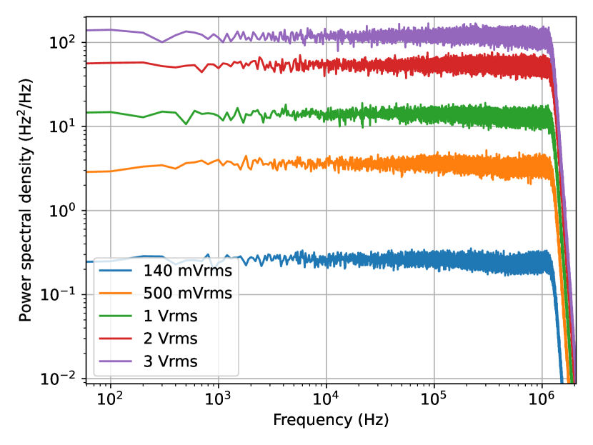
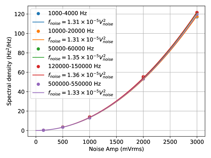
Figure 7: Amplitude calibration for the noise spectral density ($\omega_{\mathrm{noise}}$) (a) Fourier Transform of 100 averages of 0.01 seconds of data. The data is sampled at a rate of 40MHz and we have a 1MHz low pass filter. (b) Frequency averages of the data for varying white noise amplitude fitted to $f_{\textrm{noise}}=cV_{\mathrm{noise}}^{2}=\frac{\omega_{\mathrm{noise}}}{2\pi}$.

The formula resulting from Eq. (84) has a complex form, practically only possible to obtain and store using symbolic calculation software, therefore it does not provide a clear picture of the properties of the spectrum, except for making it possible to plot it numerically. In order to find the specific values of $p_{i}^{a}$, $p_{i}^{d}$, which are hidden in the formula, we use the observation that for $\Omega_{L}\gg\gamma_{i}$ the heights of the peaks in the spectrum do not depend on $\Omega_{L}$, and therefore the limits:

$$p_{i}^{a}\approx\lim_{\Omega_{L}\rightarrow+\infty}\mathrm{PSD}(\omega=\omega_{i})$$ (89)

will give, in sufficiently good approximation, the values of $p_{i}^{a}$. To obtain the approximate values of $p_{i}^{d}$, we calculate:

$$p_{i}^{d}\approx\frac{\Gamma_{i}}{\Omega_{L}}\lim_{\Omega_{L}\rightarrow+\infty}\left(\Omega_{L}\left.\frac{\mathrm{d}}{\mathrm{d}\omega}\mathrm{PSD}(\omega)\right|_{\omega=\omega_{i}}\right),$$ (90)

because we need the second order of expansion in $\frac{1}{\Omega_{L}}$. Using this approximation we obtain Eqs. (38) from the main text, and:

$$p^{d}_{1}= g_{D}^{2}\frac{3}{2}(m^{\mathrm{ini}}_{20})^{4}\frac{\omega_{\mathrm{noise}}}{\Omega_{L}}\frac{\Gamma_{0}^{2}(16\Gamma_{1}^{2}\Gamma_{2}+8\Gamma_{1}(\Gamma_{1}+5\Gamma_{2})\omega_{\mathrm{noise}}+16(\Gamma_{1}+\Gamma_{2})\omega_{\mathrm{noise}}^{2}+3\omega_{\mathrm{noise}}^{3})}{(4\Gamma_{1}+5\omega_{\mathrm{noise}})^{3}\,G(\omega_{\mathrm{noise}},\bm{\Gamma})}[3+2\cos(2\theta)+3\cos(4\theta)]^{2}$$ (91)

$$p^{d}_{2}= g_{D}^{2}\frac{9}{64}(m^{\mathrm{ini}}_{20})^{4}\frac{\omega_{\mathrm{noise}}^{2}}{\Omega_{L}}\frac{\Gamma_{0}^{2}(8\Gamma_{2}^{2}+8\Gamma_{2}\omega_{\mathrm{noise}}+\omega_{\mathrm{noise}}^{2})}{(2\Gamma_{2}+\omega_{\mathrm{noise}})^{3}\,G(\omega_{\mathrm{noise}},\bm{\Gamma})}[2\sin(2\theta)+3\sin(4\theta)]^{2}$$ (92)

where $G(\omega_{\mathrm{noise}},\bm{\Gamma})$ is stated in Eq. (39) of the main text.

C.1 Irrelevance of the dispersive contributions

We note that we have not verified the predicted relations for the dispersive contributions of the line shape, see Eq. (91) and Eq. (92) in App. C. This is due to their contribution being below the noise floor of our system. We can verify that this is as expected for a Larmor frequency of approximately 10 kHz by calculating the ratios of the peak height equations and using the linewidths found in the experiment, $\Gamma_{1}=33$ Hz and $\Gamma_{2}=30$ Hz. We find $p^{d}_{1}/p^{a}_{1}$ from Eq. (91) divided by Eq. (38b) and we find $p^{d}_{2}/p^{a}_{2}$ from Eq. (92) divided by Eq. (38c). The calculations were done for the lowest white noise amplitude of $7~{}\mathrm{mV_{rms}}$ and the highest white noise amplitude of $3.5~{}\mathrm{V_{rms}}$. For $\mathrm{V_{noise}}=7~{}\mathrm{mV_{rms}}$ we find $p^{d}_{1}/p^{a}_{1}=1.0\times 10^{-4}$ and $p^{d}_{2}/p^{a}_{2}=3.0\times 10^{-4}$. Furthermore, when $\mathrm{V_{noise}}=3.5~{}\mathrm{V_{rms}}$ we find $p^{d}_{1}/p^{a}_{1}=2.9\times 10^{-5}$ and $p^{d}_{2}/p^{a}_{2}=1.6\times 10^{-4}$. Hence, the dispersive contribution is at least 4 orders of magnitude smaller than the absorptive contribution. Hence, this is significantly below our noise floor for both peaks, as seen experimentally.

Appendix D Amplitude calibration for the noise spectral density $\omega_{\mathrm{noise}}$

In order to determine an experimental value for the constant $\omega_{\mathrm{noise}}=2\pi f_{\mathrm{noise}}=2\pi cV_{\mathrm{noise}}^{2}$ we recorded 100 0.01 second time traces of the white noise generator at varying noise amplitudes. A 1 MHz low pass filter was used to prevent the effect of aliasing. The data was then Fourier transformed to find the power spectral density. Using the power spectral density together with the coil calibration factor (10.1 $\mathrm{nT/mV_{rms}}$) and the gyromagnetic ratio of Caesium (3.5 Hz/nT) we can determine the PSD in the units of $\mathrm{Hz}^{2}/\mathrm{Hz}$. The results are shown in Fig. 7.

From Fig. 7 we can determine $f_{\mathrm{noise}}$ by seeing how the PSD varies with different white noise amplitudes. We average areas of Fig. 7 in different frequency zones and then fit this to $cV_{\mathrm{\mathrm{noise}}}^{2}$ where $V_{\mathrm{noise}}$ is in units of $\mathrm{mV_{rms}}$. Fig. 7 shows that $c=1.33(3)\times 10^{-5}$ Hz/mV${}_{\mathrm{rms}}^{2}$.

References

• Budker and Romalis [2007] D. Budker and M. Romalis, Optical magnetometryNat. Phys. 3, 227 (2007).
• Budker and Jackson Kimball [2013] D. Budker and D. F. Jackson Kimball, eds., Optical Magnetometry (Cambridge University Press, 2013).
• Kominis et al. [2003] I. K. Kominis, T. W. Kornack, J. C. Allred, and M. V. Romalis, A subfemtotesla multichannel atomic magnetometerNature 422, 596 (2003).
• [4] Gem Systems, https://www.gemsys.ca.
• [5] QuSpin, https://quspin.com.
• [6] Twinleaf, https://twinleaf.com.
• [7] Fieldline Inc., https://fieldlineinc.com.
• [8] MAG4Health, https://www.mag4health.com.
• Bison et al. [2009] G. Bison et al.A room temperature 19-channel magnetic field mapping device for cardiac signalsAppl. Phys. Lett. 95, 173701 (2009).
• Wyllie et al. [2012] R. Wyllie, M. Kauer, R. T. Wakai, and T. G. Walker, Optical magnetometer array for fetal magnetocardiographyOpt. Lett. 37, 2247 (2012).
• Jensen et al. [2018] K. Jensen, M. A. Skarsfeldt, H. Stærkind, J. Arnbak, M. V. Balabas, S.-P. Olesen, B. H. Bentzen, and E. S. Polzik, Magnetocardiography on an isolated animal heart with a room-temperature optically pumped magnetometerSci. Rep. 8, 16218 (2018).
• Xia et al. [2006] H. Xia, A. Ben-Amar Baranga, D. Hoffman, and M. V. Romalis, Magnetoencephalography with an atomic magnetometerAppl. Phys. Lett. 89, 211104 (2006).
• Boto et al. [2018] E. Boto et al.Moving magnetoencephalography towards real-world applications with a wearable systemNature 555, 657 (2018).
• Labyt et al. [2022] E. Labyt, T. Sander, and R. Wakai, eds., Flexible High Performance Magnetic Field Sensors: On-Scalp Magnetoencephalography and Other Applications (Springer, 2022).
• Marmugi and Renzoni [2016] L. Marmugi and F. Renzoni, Optical magnetic induction tomography of the heartSci. Rep. 6, 23962 (2016).
• Jensen et al. [2019] K. Jensen, M. Zugenmaier, J. Arnbak, H. Stærkind, M. V. Balabas, and E. S. Polzik, Detection of low-conductivity objects using eddy current measurements with an optical magnetometerPhys. Rev. Res. 1, 033087 (2019).
• Wickenbrock et al. [2016] A. Wickenbrock, N. Leefer, J. W. Blanchard, and D. Budker, Eddy current imaging with an atomic radio-frequency magnetometerAppl. Phys. Lett. 108, 183507 (2016).
• Bevington et al. [2019] P. Bevington, R. Gartman, and W. Chalupczak, Enhanced material defect imaging with a radio-frequency atomic magnetometerJ. Appl. Phys. 125, 094503 (2019).
• Deans et al. [2018] C. Deans, L. Marmugi, and F. Renzoni, Active underwater detection with an array of atomic magnetometersAppl. Optics 57, 2346 (2018).
• Rushton et al. [2022] L. M. Rushton, T. Pyragius, A. Meraki, L. Elson, and K. Jensen, Unshielded portable optically pumped magnetometer for the remote detection of conductive objects using eddy current measurementsRev. Sci. Instrum. 93, 125103 (2022).
• Wasilewski et al. [2010] W. Wasilewski, K. Jensen, H. Krauter, J. J. Renema, M. V. Balabas, and E. S. Polzik, Quantum noise limited and entanglement-assisted magnetometryPhys. Rev. Lett. 104, 133601 (2010).
• Chalupczak et al. [2012] W. Chalupczak, R. M. Godun, S. Pustelny, and W. Gawlik, Room temperature femtotesla radio-frequency atomic magnetometerAppl. Phys. Lett. 100, 242401 (2012).
• Keder et al. [2014] D. A. Keder, D. W. Prescott, A. W. Conovaloff, and K. L. Sauer, An unshielded radio-frequency atomic magnetometer with sub-femtotesla sensitivityAIP Adv. 4, 127159 (2014).
• Ledbetter et al. [2007] M. P. Ledbetter, V. M. Acosta, S. M. Rochester, D. Budker, S. Pustelny, and V. V. Yashchuk, Detection of radio-frequency magnetic fields using nonlinear magneto-optical rotationPhys. Rev. A 75, 023405 (2007).
• Rushton et al. [2023] L. M. Rushton, L. Elson, A. Meraki, and K. Jensen, Alignment-based optically pumped magnetometer using a buffer-gas cell, Phys. Rev. Appl. 19, 064047 (2023).
• Happer [1972] W. Happer, Optical pumpingRev. Mod. Phys. 44, 169 (1972).
• Weis et al. [2006] A. Weis, G. Bison, and A. S. Pazgalev, Theory of double resonance magnetometers based on atomic alignmentPhys. Rev. A 74, 033401 (2006).
• Zigdon et al. [2010] T. Zigdon, A. D. Wilson-Gordon, S. Guttikonda, E. J. Bahr, O. Neitzke, S. M. Rochester, and D. Budker, Nonlinear magneto-optical rotation in the presence of a radio-frequency field, Opt. Express 18, 25494 (2010).
• Beato et al. [2018] F. Beato, E. Belorizky, E. Labyt, M. Le Prado, and A. Palacios-Laloy, Theory of a ${}^{4}\mathrm{He}$ parametric-resonance magnetometer based on atomic alignmentPhys. Rev. A 98, 053431 (2018).
• Bertrand et al. [2021] F. Bertrand, T. Jager, A. Boness, W. Fourcault, G. Le Gal, A. Palacios-Laloy, J. Paulet, and J. M. Léger, A ${}^{4}\mathrm{He}$ vector zero-field optically pumped magnetometer operated in the earth-fieldRev. Sci. Instr. 92, 105005 (2021).
• Colangelo et al. [2013] G. Colangelo, R. J. Sewell, N. Behbood, F. M. Ciurana, G. Triginer, and M. W. Mitchell, Quantum atom-light interfaces in the gaussian description for spin-1 systemsNew J. Phys. 15, 103007 (2013).
• Auzinsh et al. [2014] M. Auzinsh, D. Budker, and S. M. Rochester, Optically Polarized Atoms: Understanding Light-Atom Interactions (Oxford University Press, 2014).
• Sinitsyn and Pershin [2016] N. A. Sinitsyn and Y. V. Pershin, The theory of spin noise spectroscopy: A review, Rep. Prog. Phys. 79, 106501 (2016).
• Gardiner and Zoller [2000] C. Gardiner and P. Zoller, Quantum Noise (Springer, 2000).
• Zapasskii et al. [2013] V. S. Zapasskii, A. Greilich, S. A. Crooker, Y. Li, G. G. Kozlov, D. R. Yakovlev, D. Reuter, A. D. Wieck, and M. Bayer, Optical spectroscopy of spin noisePhys. Rev. Lett. 110, 176601 (2013).
• Glasenapp et al. [2014] P. Glasenapp, N. A. Sinitsyn, L. Yang, D. G. Rickel, D. Roy, A. Greilich, M. Bayer, and S. A. Crooker, Spin noise spectroscopy beyond thermal equilibrium and linear responsePhys. Rev. Lett. 113, 156601 (2014).
• Shah et al. [2010] V. Shah, G. Vasilakis, and M. V. Romalis, High bandwidth atomic magnetometery with continuous quantum nondemolition measurementsPhys. Rev. Lett. 104, 013601 (2010).
• Lucivero et al. [2016] V. G. Lucivero, R. Jiménez-Martínez, J. Kong, and M. W. Mitchell, Squeezed-light spin noise spectroscopyPhys. Rev. A 93, 053802 (2016).
• Fomin et al. [2020] A. A. Fomin, M. Y. Petrov, G. G. Kozlov, M. M. Glazov, I. I. Ryzhov, M. V. Balabas, and V. S. Zapasskii, Spin-alignment noise in atomic vaporPhys. Rev. Res. 2, 012008 (2020).
• Fomin et al. [2021] A. A. Fomin, M. Y. Petrov, I. I. Ryzhov, G. G. Kozlov, V. S. Zapasskii, and M. M. Glazov, Nonlinear spectroscopy of high-spin fluctuationsPhys. Rev. A 103, 023104 (2021).
• Liu et al. [2022] S. Liu, P. Neveu, J. Delpy, L. Hemmen, E. Brion, E. Wu, F. Bretenaker, and F. Goldfarb, Birefringence and dichroism effects in the spin noise spectra of a spin-1 systemNew J. Phys. 24, 113047 (2022).
• Liu et al. [2023] S. Liu, P. Neveu, J. Delpy, E. Wu, F. Bretenaker, and F. Goldfarb, Spin-noise spectroscopy of a spin-one systemPhys. Rev. A 107, 023527 (2023).
• Delpy et al. [2023a] J. Delpy, S. Liu, P. Neveu, E. Wu, F. Bretenaker, and F. Goldfarb, Spin-noise spectroscopy of optical light shiftsPhys. Rev. A 107, L011701 (2023a).
• Delpy et al. [2023b] J. Delpy, S. Liu, P. Neveu, C. Roussy, T. Jolicoeur, F. Bretenaker, and F. Goldfarb, Creation and dynamics of spin fluctuations in a noisy magnetic fieldNew J. Phys. 25, 093055 (2023b).
• Note [1] In contrast to the parallel configuration, in which the white noise would just yield effective fluctuations of the static field [44].
• Jiménez-Martínez et al. [2018] R. Jiménez-Martínez, J. Kołodyński, C. Troullinou, V. G. Lucivero, J. Kong, and M. W. Mitchell, Signal tracking beyond the time resolution of an atomic sensor by kalman filteringPhys. Rev. Lett. 120, 040503 (2018).
• Kitching [2018] J. Kitching, Chip-scale atomic devicesApp. Phys. Rev. 5, 031302 (2018).
• Rochester and Budker [2001] S. M. Rochester and D. Budker, Atomic polarization visualizedAmerican Journal of Physics 69, 450 (2001).
• Deutsch and Jessen [2010] I. H. Deutsch and P. S. Jessen, Quantum control and measurement of atomic spins in polarization spectroscopyOpt. Commun. 283, 681 (2010).
• Savukov and Romalis [2005] I. M. Savukov and M. V. Romalis, Effects of spin-exchange collisions in a high-density alkali-metal vapor in low magnetic fieldsPhys. Rev. A 71, 023405 (2005).
• Savukov [2017] I. M. Savukov, Spin exchange relaxation free (serf) magnetometers, in High Sensitivity Magnetometers, edited by A. Grosz, M. J. Haji-Sheikh, and S. C. Mukhopadhyay (Springer International Publishing, 2017) pp. 451–491.
• Mouloudakis and Kominis [2021] K. Mouloudakis and I. K. Kominis, Spin-exchange collisions in hot vapors creating and sustaining bipartite entanglementPhys. Rev. A 103, L010401 (2021).
• Katz et al. [2022] O. Katz, R. Shaham, and O. Firstenberg, Quantum interface for noble-gas spins based on spin-exchange collisionsPRX Quantum 3, 010305 (2022).
• Bevilacqua et al. [2014] G. Bevilacqua, E. Breschi, and A. Weis, Steady-state solutions for atomic multipole moments in an arbitrarily oriented static magnetic fieldPhys. Rev. A 89, 033406 (2014).
• Breuer and Petruccione [2002] H.-P. Breuer and F. Petruccione, The Theory of Open Quantum Systems (Oxford University Press, 2002).
• Gardiner et al. [1985] C. W. Gardiner et al.Handbook of Stochastic Methods, Vol. 3 (springer Berlin, 1985).
• Note [2] Even if $\theta^{\prime}$ is not exactly matched, the resulting DC-component of the detected signal (27) yields a spike at zero frequency in the PSD, whose presence may be safely ignored within our analysis.
• Note [3] Eq. (30) could be equivalently defined in terms of the auto-correlation function of $\delta S(t)=S(t)-\left\langle S(t)\right\rangle$ [56].
• Wilson et al. [2020] N. Wilson, C. Perrella, R. Anderson, A. Luiten, and P. Light, Wide-bandwidth atomic magnetometry via instantaneous-phase retrievalPhys. Rev. Res. 2, 013213 (2020).
• Li et al. [2020] R. Li, F. N. Baynes, A. N. Luiten, and C. Perrella, Continuous high-sensitivity and high-bandwidth atomic magnetometerPhys. Rev. Appl. 14, 064067 (2020).
• Hao et al. [2022] S. Hao, H. Shi, C. N. Gagatsos, M. Mishra, B. Bash, I. Djordjevic, S. Guha, Q. Zhuang, and Z. Zhang, Demonstration of entanglement-enhanced covert sensingPhys. Rev. Lett. 129, 010501 (2022).
• Troullinou et al. [2021] C. Troullinou, R. Jiménez-Martínez, J. Kong, V. G. Lucivero, and M. W. Mitchell, Squeezed-light enhancement and backaction evasion in a high sensitivity optically pumped magnetometerPhys. Rev. Lett. 127, 193601 (2021).
• Lucivero et al. [2017] V. G. Lucivero, A. Dimic, J. Kong, R. Jiménez-Martínez, and M. W. Mitchell, Sensitivity, quantum limits, and quantum enhancement of noise spectroscopiesPhys. Rev. A 95, 041803 (2017).