Radiation-reaction effects on the production of twisted photon in the nonlinear inverse Thomson scattering

Abstract

Twisted photons can be emitted by free electrons in circular or spiral motion, which carry orbital angular momentum (OAM) and possess a helical phase structure. However, classical radiation reaction (RR) effects has not been investigated as an accelerated electron emits vortex radiation during the interaction with a laser. This work focuses on investigating the effects of radiation reaction on the production of twisted photons in the Nonlinear Inverse Thomson Scattering (NITS) process. Using the precise electron trajectory obtained by Landau-Lifshitz (LL) equation with a circularly polarized (CP) laser, we find that the radiation reaction effects can be significant for a sufficiently long pulse of a laser. They observe modifications in the frequency, phase structure, rotational asymmetry of OAM density, and energy distribution of the vortex field due to radiation reaction. This finding could provide an unique signature for the detection of radiation reaction.

I Introduction

Free electrons in circular or spiral motion can emit twisted photons naturally carrying well-defined orbital angular momentum (OAM) [1, 2, 3]. This discovery indicates that an electromagnetic wave radiated by a single free electron in circular motion or a spiral motion has a helical phase structure and carries OAM. Since the twisted photon can be emitted by the classical radiation in the context of real physical processes, the vortex gamma-ray source could be available via the laser-electron interaction or a helical undulator [4, 5]. The potential applications of twisted photons are vast and varied [6]. Twisted photons can be used to study the properties of materials and to manipulate the spin and orbital angular momentum of particles [7, 8, 9]. Besides, twisted photons play a vital role in understanding radiation mechanism in astrophysics [10, 11]. The discovery of twisted photons emitted by free electrons opens up new avenues for research and has the potential to revolutionize many fields of science and technology.

Precisely, for the interaction between an ultrarelativistic electron and a relativistic laser with intermediate intensity, or nonlinear inverse Thomson scattering (NITS) process, the electron trajectory should be described by considering the classical radiation reaction (RR) effects. RR describes the motion of charged particles in the presence of electromagnetic fields, and arises from the fact that a charged particle that is accelerated in an electromagnetic field will emit radiation, and this radiation will carry away energy and momentum from the particle [12, 13, 14, 15]. This leads to a back-reaction force on the particle, which can affect its motion and thus the radiation. Neglecting the quantum effects, the radiation-reaction force in the instantaneous rest frame of the electron is always much weaker than the Lorentz force, and Landau-Lifshitz (LL) equation is effective to describe the motion of a charged particle in an electromagnetic field, including the effects of radiation reaction [16, 17]. Although LL equation has limitations and are not applicable in all situations, particularly at ultraintense field where quantum effects become important [18, 19, 20], classical RR provides a foundation for understanding the radiation behavior of charged particles in electromagnetic fields. Therefore, radiation reaction effects on the vortex radiation can be taken into account via the LL equation [21, 22, 17].

In this paper, we theoretically investigate the RR effects on the production of twisted photons in the NITS process. Utilizing the precise electron spiral trajectory of LL equation for the interaction between a electron and a circularly polarized (CP) laser, the dominate RR effects are connected to the number of laser cycles. By using tens of thousand laser cycles, RR effects can be large and the radiation remains below the threshold for quantum effects. The vortex fields resulting from RR modified electron trajectory can be obtained for each harmonic. We find that RR can lead to the inconsistence between center frequency and resonant frequency, and modifies the phase structure of vortex field to the Bessel mode. Moreover, RR breaks the rotation symmetry of the vortex field and thus the angular momentum in transverse plane, and compared to the case without RR, enhances the energy density of each harmonic and reallocate the proportions of energy on high-order harmonics energy.

The paper is organized as follows: In Sec. II, we derive the precise trajectory using LL equation and the corresponding harmonic radiation field using Lienard-Wiechert potential. In Sec. III, the numerical results about the RR effects on the OAM photons are discussed. Finally, we present a concise summary of our findings in Sec. IV.

II Theoretical derivation of the radiation-reaction effects in the NITS

II.1 The precise trajectory of an electron in NITS with a circularly polarized light

Assuming the experienced RR of an electron can be described by the Landau–Lifshitz (LL) equation, we consider the interaction of an electron with a plane-wave electromagnetic field, and to obtain the analytical trajectories, invoke the exact solution of the LL equation [21]. The trajectories are obtained in the Cartesian coordinate system $(x,y,z)$, wherein a circularly polarized (CP) laser propagates along the $-\hat{\bm{z}}$ direction and an electron moves along the $+\hat{\bm{z}}$ direction. The international unit is used throughout the paper. The four-vector potential of a left-hand CP laser is designated as

$$\mathbf{A}(\eta) = (E_{0}/k_{0}c)\left[\cos(k_{0}\eta)\bm{e}_{x}+\sin(k_{0}\eta)\bm{e}_{y}\right],$$ (1)

where $\eta=z+ct$ serves as an independent variable describing the motion of the electron. $E_{0}$ is the amplitude of electric field and normalized as $a_{0}=E_{0}e/mc\omega_{0}$, and $k_{0}=\omega_{0}/c=2\pi/\lambda_{0}$ is the wave number corresponding to frequency $\omega_{0}$ and wavelength $\lambda_{0}$ of the CP laser.

Denoting $\eta_{0}$ as the initial value of $\eta$, and the length of a plane-wave laser as $\ell_{0}=N_{0}\lambda_{0}$ with the number of laser cycles $N_{0}$. According to the exact solution of LL equation for the four-vector velocity $u^{\mu}$, the corresponding trajectory $\bm{r}_{e}=(x_{e},y_{e},z_{e})$ of an electron, with initial position ($x_{0},y_{0},z_{0}$) and $\rho_{0}=\gamma_{0}(1+\beta_{0})$, can be obtained via $x^{\mu}=x^{\mu}_{0}+\frac{1}{\rho_{0}}\int_{\eta_{0}}^{\eta}h(\eta)u^{\mu}(\eta)d\eta$, expressed as

$$x_{e} =x_{0}+r_{1}\left[\sin{(k_{0}\eta)}\left(1+\frac{2}{3}R_{c}k_{0}(\eta-\eta_{0})\right)\right.$$

$$\quad+\left.\frac{4}{3}R_{c}\cos{(k_{0}\eta)}+\frac{2}{3}\alpha\frac{k_{0}\rho_{0}}{m}\cos{(k_{0}\eta)}\right.$$

$$\quad+\left.\frac{2}{3}R_{c}\omega_{0}(\phi-\phi_{0})\sin{(k_{0}\eta_{0})}\right],$$ (2a)

$$y_{e} =y_{0}-r_{1}\left[\cos{(k_{0}\eta)}\left(1+\frac{2}{3}R_{c}k_{0}(\eta-\eta_{0})\right)\right.$$

$$\quad+\left.\frac{4}{3}R_{c}\sin{(k_{0}\eta)}+\frac{2}{3}\alpha\frac{k_{0}\rho_{0}}{m}\sin{(k_{0}\eta)}\right.$$

$$\quad+\left.\frac{2}{3}R_{c}\omega_{0}(\phi-\phi_{0})\cos{(k_{0}\eta_{0})}\right],$$ (2b)

$$z_{e} =z_{0}+\beta_{1}k_{0}(\eta-\eta_{0})+\beta_{2}[k_{0}(\eta-\eta_{0})]^{2}$$

$$\quad+\beta_{3}[k_{0}(\eta-\eta_{0})]^{3}+\beta_{4}\sin{(k_{0}\eta)}+\beta_{5}\cos{(k_{0}\eta)},$$ (2c)

where $\alpha$ is the fine-structure constant, and $R_{c}=\alpha k_{0}\gamma_{0}(1+\beta_{0})a_{0}^{2}/2m$ the invariant classical radiation reaction parameter which controls the magnitude of the radiation losses percycle. Parameters $r_{1}$ and $\beta_{1}$ above are

$$r_{1} = \frac{a_{0}}{\sqrt{2}\gamma_{0}(1+\beta_{0})k_{0}},$$ (3)

$$\beta_{1} = \frac{1}{2}\left(1-\frac{1+\frac{a_{0}^{2}}{2}+\frac{4}{9}R_{c}^{2}}{2\gamma_{0}^{2}(1+\beta_{0})^{2}k_{0}}\right),$$ (4)

respectively, and parameters $\beta_{2}$, $\beta_{3}$, $\beta_{4}$, and $\beta_{5}$ above are

$$\beta_{2}=-\frac{\frac{4}{3}R_{c}a_{0}^{2}}{2\rho_{0}^{2}k_{0}},\beta_{3}=-\frac{\frac{4}{9}R_{c}^{2}a_{0}^{2}}{2\rho_{0}^{2}k_{0}},\beta_{4}=\frac{\frac{4}{9}R_{c}^{2}a_{0}^{2}}{2\rho_{0}^{2}k_{0}},\beta_{5}=\frac{\frac{4}{3}R_{c}a_{0}^{2}}{2\rho_{0}^{2}k_{0}},$$ (5)

respectively. Here, $a_{0}=eE_{0}/m\omega_{0}c$ is the laser intensity, $\gamma_{0}$ and $\beta_{0}$ are the initial relativistic factor and velocity of an electron.

Eq. (2) indicates that for the dominant order, the RR effects can be characterized by the term $R_{c}k_{0}(\eta-\eta_{0})$, and it would be large in long laser pulses while remaining below the threshold for quantum effects. When $R_{c}k_{0}(\eta-\eta_{0})\ll 1$, the above trajectories in Eq (2) recover to the normal helical motion with constant radius $r_{1}$. Therefore, the RR effects described by LL equation can be significant when $R_{c}k_{0}(\eta-\eta_{0})\sim 1$ is available via a sufficiently long duration $(\eta-\eta_{0})$ of a laser. Neglecting the minor terms associated to the laser intensity $a_{0}$, Eq. (2) can be approximated as

$$x \simeq x_{0}+r_{1}\left[\sin(k_{0}\eta)+\frac{2}{3}R_{c}k_{0}(\eta-\eta_{0})\left[\sin{(k_{0}\eta)}+\sin{(k_{0}\eta_{0})}\right]\right],$$ (6a)

$$y \simeq y_{0}-r_{1}\left[\cos(k_{0}\eta)+\frac{2}{3}R_{c}k_{0}(\eta-\eta_{0})\left[\cos{(k_{0}\eta)}+\cos{(k_{0}\eta_{0})}\right]\right],$$ (6b)

$$z \simeq z_{0}+\beta_{1}k_{0}(\eta-\eta_{0}),$$ (6c)

which describes the classical RR effects dominated by the interaction duration.

II.2 The harmonic radiation field with RR effects in NITS

The radiation field from NITS can be calculated by the Lienard-Wiechert potential, which results in the Fourier components of the electric field emitted by a single electron in any orbit $\bm{r}_{e}$ with a normalized velocity $\beta=v/c$, and is expressed as [4]

$$\bm{E}=-i\sqrt{\dfrac{e^{2}k^{2}}{32\pi^{3}\varepsilon_{0}^{2}}}\dfrac{e^{ikR}}{R}\int_{-\infty}^{\infty}dt\{\bm{n}\times(\bm{n}\times\beta)\}e^{i\omega\left(t-\frac{\bm{n}\cdot\bm{r}_{e}(t)}{c}\right)},$$ (7)

where e is the elementary charge and $\varepsilon_{0}$ the vacuum dielectric constant. $\omega$ and $k=\omega/c$ are the angular frequency and wave number of the emitted photons, respectively, and $R$ the distance from the origin to the observation point with the direction $\bm{n}$.

It is convenient to calculate Eq. (7) in the spherical coordinates $(r,\theta,\phi)$. Following the method of Ref. [4] and substituting the trajectories of Eq. (6) into Eq. (7), the $\theta$ and $\phi$ components, $E_{\theta}$ and $E_{\phi}$, of the radiation field are obtained as

$$E_{\theta} = \sum_{n=1}^{+\infty}i\sqrt{\frac{e^{2}k^{2}}{32\pi^{3}\varepsilon_{0}^{2}c^{2}}}\frac{e^{ikR+in\phi+i\psi_{0}}}{R}e^{-ink_{0}\eta_{0}}\int_{-\ell_{0}/2}^{\ell_{0}/2}d\eta$$ (8)

$$\times \left\{\left[\frac{nk_{0}cos\theta}{ksin\theta}+\frac{2}{3}R_{c}k_{0}r_{1}sin\sigma-\beta_{1}sin\theta\right]J_{n}(p_{c})\right.$$

$$+ \left.i\frac{2}{3}R_{c}k_{0}r_{1}J^{\prime}_{n}(p_{c})\right\}e^{-i\bar{k}_{c}(\eta-\eta_{0})},$$

$$E_{\phi} = \sum_{n=1}^{+\infty}-\sqrt{\frac{e^{2}k^{2}}{32\pi^{3}\varepsilon_{0}^{2}c^{2}}}\frac{e^{ikR+in\phi+i\psi_{0}}}{R}e^{-ink_{0}\eta_{0}}\int_{-\ell_{0}/2}^{\ell_{0}/2}d\eta$$ (9)

$$\times \left\{k_{0}r_{1}\mathcal{N}J^{\prime}_{n}(p_{c})+\frac{2}{3}R_{c}k_{0}r_{1}\frac{n}{p_{c}}J_{n}(p_{c})\right.$$

$$+ \left.\frac{2}{3}R_{c}k_{0}r_{1}\cos\sigma J_{n}(p_{c})\right\}e^{-i\bar{k}_{c}(\eta-\eta_{0})},$$

with $\sigma\equiv k_{0}\eta-\phi$ ($\sigma_{0}=k_{0}\eta_{0}-\phi$) and $\mathcal{N}\equiv\left[1+\frac{2}{3}R_{c}k_{0}(\eta-\eta_{0})\right]$, and

$$\bar{k}_{c} \equiv k[1-\beta_{1}(1+\cos{\theta})]-\frac{2}{3}R_{c}k_{0}p\sin{\sigma_{0}}-nk_{0},$$ (10)

$$p_{c} \equiv kr_{1}\sin{\theta}\mathcal{N},$$ (11)

$$\psi_{0} \equiv -k\left[x_{0}\sin{\theta}\cos{\phi}+y_{0}\sin{\theta}\sin{\phi}+z_{0}(1+\cos{\theta})\right].$$ (12)

The detailed derivation of Eqs. (8) and (9) is presented in the Appendix A.

Considering $R_{c}\ll 1$, $E_{\theta}$ and $E_{\phi}$ can be approximated as

$$E_{\theta} \simeq \sum_{n}i\sqrt{\frac{e^{2}k^{2}}{32\pi^{3}\varepsilon_{0}^{2}c^{2}}}\frac{e^{ikR+in\phi+i\psi_{0}-ink_{0}\eta_{0}}}{R}\left[\frac{nk_{0}cos\theta}{ksin\theta}-\beta_{1}sin\theta\right]$$ (13)

$$\times \int_{-\ell_{0}/2}^{\ell_{0}/2}d\eta J_{n}(p_{c})e^{-i\bar{k}_{c}(\eta-\eta_{0})},$$

$$E_{\phi} \simeq \sum_{n}-\sqrt{\frac{e^{2}k^{2}}{32\pi^{3}\varepsilon_{0}^{2}c^{2}}}\frac{e^{ikR+in\phi+i\psi_{0}-ink_{0}\eta_{0}}}{R}k_{0}r_{1}$$ (14)

$$\times \int_{-\ell_{0}/2}^{\ell_{0}/2}d\eta\mathcal{N}J^{\prime}_{n}(p_{c})e^{-i\bar{k}_{c}(\eta-\eta_{0})}.$$

When $R_{c}=0$, the radiation fields expressed in Eqs. (13) and (14) recover to the ones obtained in Ref. [4].

Substituting the integer-order Bessel function into the above equations and using the following integration formula:

$$\int x^{n}e^{-ikx}dx=-\frac{1}{(ik)^{n+1}}\Gamma(n+1,ikx)+\rm{constant},$$ (15)

$E_{\theta}$ and $E_{\phi}$ can be arranged into the following compact forms:

$$E_{\theta} \simeq \frac{e^{ikR}}{R}\sum_{n}iC_{\theta,n}e^{in\phi-ink_{0}\eta_{0}+i\psi_{0}},$$ (16)

$$E_{\phi} \simeq \frac{e^{ikR}}{R}\sum_{n}-C_{\phi,n}e^{in\phi-ink_{0}\eta_{0}+i\psi_{0}}.$$ (17)

The concrete expressions of $C_{\theta,n}$ and $C_{\phi,n}$ are presented in the Appendix A. To show the phase structure of radiation field in the transverse plane, the electric fields in Eqs. (16) and (17) can be transformed to $E_{x}\bm{e}_{x}$ and $E_{y}\bm{e}_{y}$ in the Cartesian coordinate [4], resulting in

$$E_{\pm}=\frac{E_{x}\pm iE_{y}}{\sqrt{2}}=\frac{e^{ikR}}{R}\sum_{n}C_{\pm,n}e^{i(n\mp 1)\phi-ink_{0}\eta_{0}+i\psi_{0}},$$ (18)

for the helicity components $\bm{e}_{\pm}=(\bm{e}_{x}\pm i\bm{e}_{y})/\sqrt{2}$. Defining $\varphi_{\pm,n}$ as the vortex phase of nth harmonic, it has

$$\varphi_{\pm,n}=\tan{n(\phi-k_{0}\eta_{0}+\psi_{0})}\arctan{\frac{\mathfrak{Im}(C_{\pm,n})}{\mathfrak{Re}(C_{\pm,n})}}.\\$$ (19)

II.3 Broadening resonance function due to RR effects

Resonance function determines the bandwidth of the radiation spectrum for a given harmonic and reflects the properties of the harmonic electric field peak. With RR effects, the resonance functions can also be defined by the normalized integral parts of Eqs. (13) and (14), namely,

$$\mathcal{R}_{\theta} =\left|\frac{\int_{-\ell_{0}/2}^{\ell_{0}/2}J_{n}(p_{c})e^{i\bar{k}_{c}(\eta-\eta_{0})}d\eta}{\int_{-\ell_{0}/2}^{\ell_{0}/2}J_{n}(p_{c})d\eta}\right|^{2},$$ (20a)

$$\mathcal{R}_{\phi} =\left|\frac{\int_{-\ell_{0}/2}^{\ell_{0}/2}\mathcal{N}J^{\prime}_{n}(p_{c})e^{i\bar{k}_{c}(\eta-\eta_{0})}d\eta}{\int_{-\ell_{0}/2}^{\ell_{0}/2}\mathcal{N}J^{\prime}_{n}(p_{c})d\eta}\right|^{2},$$ (20b)

for the radiation field along $\theta$ and $\phi$ directions. When $R_{c}=0$, Eq. (38) recovers to the form of $\mathcal{R}(k,nk_{0})=|\frac{sin(\bar{k}\eta_{0})}{\bar{k}\eta_{0}}|^{2}$ for the radiation fields without RR effects [23], where $\bar{k}=k[{1-\beta_{1}(1+cos\theta)}]-{nk_{0}}$.

The properties of $\mathcal{R}_{\theta}$ and $\mathcal{R}_{\phi}$ are dependent on the variable $p_{c}$, which has the maximum of $p_{m}=kr_{1}\sin{\theta}(1+\frac{4}{3}\pi R_{c}N_{0})$ when $\eta-\eta_{0}=\ell_{0}$, and the nonzero $R_{c}$ of $p_{m}$ causes the dependence on the number of laser cycle $N_{0}$. Denoting $\alpha_{1}^{(n)}$ as the first zero point of $J_{n}(p_{c})$, when $p_{m}<\alpha_{1}^{(n)}$, it can be proved that $\mathcal{R}_{\theta}$ has the maximum value at $\bar{k}_{c}=0$ (see the details in the Appendix A). Similarly, and $\mathcal{R}_{\phi}$ has the maximum value at $\bar{k}_{c}=0$ when $p_{m}<\beta_{1}^{(n)}$, where $\beta_{1}^{(n)}$ is the first zero point of $J^{\prime}_{n}(p_{c})$. From $\bar{k}_{c}=0$, the wave number of the radiation field is obtained as

$$k=\dfrac{nk_{0}}{1-\beta_{1}(1+\cos\theta)-\frac{2}{3}R_{c}k_{0}r_{1}\sin\theta\sin\sigma_{0}},$$ (21)

which implies that RR can cause the extra frequency shift of the radiation fields. The equivalent evidence is that when $p_{m}>\alpha_{1}^{(n)}$, $\mathcal{R}_{\theta}$ and $\mathcal{R}_{\phi}$ will not be maximum at $\bar{k}_{c}=0$, and actually, will split into two peaks according to the numerical calculation (see the discussions in Fig. 1 below).

III Numerical results of RR effects on the emission of vortex gamma-ray photons

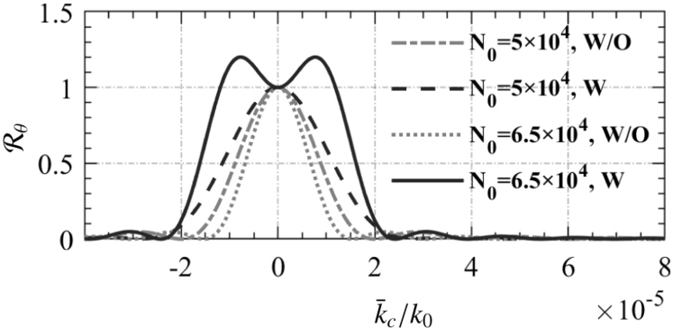
FIG 1: Resonance function $\mathcal{R}_{\theta}$ with $n=1$ versus $\bar{k}_{c}/k_{0}$, corresponding to the number of the laser-electron interacting periods of $N_{0}=5\times 10^{4}$ and $N_{0}=6.5\times 10^{4}$ with (W) and without (W/O) RR effects. The results are obtained by using Eq. (38).

In the numerically investigation of the classical RR effects, $R_{c}\ll 1$ and $\chi\ll 1$ should be fulfilled so that classical RR can be a good approximation to quantum RR for a given set of parameters of laser and electron [12]. For this end, we consider an incident electron energy of 1 GeV (i.e., $\gamma_{0}=2000$, $\rho_{0}=\gamma_{0}(1+\beta_{0})=4000$), CP laser intensity of $a_{0}=1$ and the number of laser cycles of $N_{0}=10^{4}$. This set of parameters results in $R_{c}\simeq 10^{-4}$, $\chi=\frac{a_{0}\gamma_{0}(1+\beta_{0})k_{0}}{m}\simeq 0.008$, and $\frac{2}{3}R_{c}k_{0}(\eta-\eta_{0})\simeq 1$ in Eq. (6), which implies that RR effects is non-negligible in this considered scenario.

The difference between the amplitudes of $\mathcal{R}_{\theta}$ and $\mathcal{R}_{\phi}$ is negligible for the considered parameters, which implies that the spatial inhomogeneity of radiation amplitude $|E_{\theta}|^{2}+|E_{\phi}|^{2}$ induced by RR is negligible. $\mathcal{R}_{\theta}$ is used to illustrate the RR effects on bandwidth of radiation field; see Fig. 1. Without RR, the bandwidth becomes narrow as $N_{0}$ increases since $\Delta\omega=1/nN_{0}$, and the central frequency of a harmonic equals the resonant frequency determined at $\bar{k}=0$ or the peak of resonance function. However, the bandwidth is broaden by RR, and the broadening of bandwidth becomes wide with increasing $N_{0}$ which enhances the strength of RR. Moreover, when $p_{m}>\mu_{1}^{(n)}$, $\mathcal{R}_{\theta}$ is available at $N_{0}=6.5\times 10^{4}$, $R_{\theta}$ is split into two peaks beside $\bar{k}_{c}=0$. The split resonance function indicates that the resonance peak of radiation field for a harmonic is not determined at $\bar{k}_{c}=0$, and RR can result in two resonance frequencies for a harmonic. For the higher harmonics with $n>1$, the variation of resonance function with $\bar{k}_{c}$ is similar to the case of first harmonic.

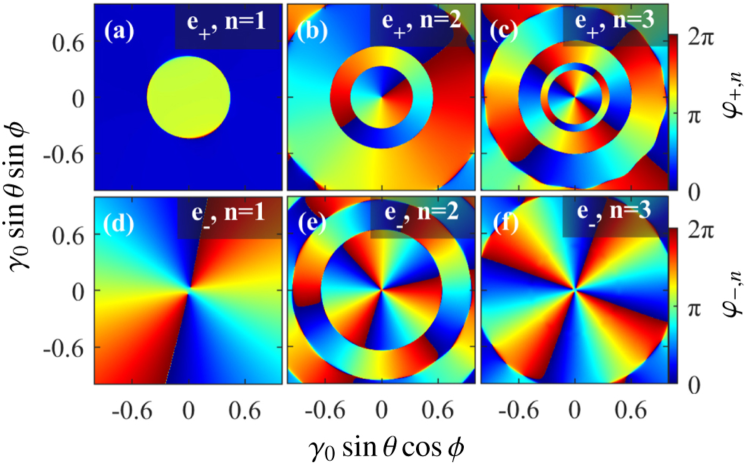
FIG 2: Spatial distributions of the phase of the radiation field with positive ($e_{+}$) and negative ($e_{-}$) helicity components for: (a) first, (b) second, and (c) third harmonics. (d)-(f) similar to (a)-(c) but for the $e_{-}$ component of radiation field. The results are calculated by Eq. (19) with $N_{0}=2.4\times 10^{4}$.

The phase structure of a twisted photon is shown in Eq. (18), and the phase term $e^{i(n\mp 1)\phi}$ represents the carried number of OAM for the CP components with positive and negative helicities. However, parameter $\mathcal{N}$ is dependent on $\eta$ due to nonzero $R_{c}$, the integration of $J_{n}(p_{c})$ and its derivative $J^{\prime}_{n}(p_{c})$ in Eqs. (8) and (9) leads to the complex amplitude $C_{\pm,n}$. Therefore, the phase structure of a twisted photon can be modulated by RR. For the case of the single-peaked resonance function, RR effect on phase structure is negligible. However, when resonance function is bimodal distribution for a sufficiently long laser cycles, the phase structure is significantly modulated as the Bessel model, i.e., the relative phases occur the loop structure; See Fig. 2. When $N_{0}$ increases, the loop phase for vortex charge $n=2,3,\ldots$ grows inward for $\bm{e}_{+}$ component [see Figs. 2 (b) and (c)] and grows outward for $\bm{e}_{-}$ component [see Figs. 2 (e) and (f)]. Because the interaction of a left-hand CP laser with a electron results in the trajectory fo left-hand spiral, the relative phases of the twisted photon grow around the circle anticlockwise and form a vortex $\exp{(in\phi)}$ with phase increment $n2\pi$ around the loop.

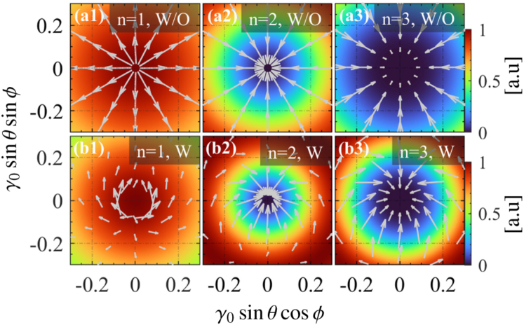
FIG 3: Spatial distributions of the normalized spectra $d^{2}I/d\omega d\Omega$ from NITS for different harmonics: (a1)-(a3) without (W/O), and (b1)-(b3) with (W) RR effects. The time-averaged OAM density $\langle\bm{j}\rangle$ for each harmonic is superposed onto the spectra. The results are calculated by Eqs. (13), (14) and (22) with $N_{0}=2.4\times 10^{4}$.

As is clarified that electric filed of harmonic is modified by Bessel function due to RR [see Eqs. (13) and (14)], thus the corresponding spectra, namely, the radiation energy per angular frequency and solid angle $d^{2}I/d\omega d\Omega=2\varepsilon_{0}R^{2}(|E_{\theta}|^{2}+|E_{\phi}|^{2})$, can be modified by RR. To reveal that, the spatial distributions of spectra without and with RR for each harmonic are compared; see Fig. 3. For the first harmonic, RR leads to the more focused energy spot [see Figs. 3(a1) and (b1)]. For the higher harmonics, RR leads to the more concentrated energy distribution around z-axis, i.e., the radius of annular intensity profiles, defined as the radial distance between the singularity spot and the peak, with RR is smaller. The time-averaged OAM density $\langle\bm{j}\rangle$ of radiation field is defined as [2]:

$$\langle\bm{j}\rangle=\bm{r}\times\langle\bm{p}\rangle=\frac{R}{4\pi c}\left[\bm{E}(\bm{n}\cdot\bm{H}^{*})-\bm{H}(\bm{n}\cdot\bm{E}^{*})\right].$$ (22)

Substituting the electric field of each harmonic in Eqs. (13) and (14) into Eq. (22), the RR effects on the vortex field can be directly revealed via OAM density. The detailed derivation of $\langle\bm{j}\rangle$ is presented in the Appendix B). Eq. (22) shows that the direction of OAM is determined by the direction of the electric and magnetic fields. Without RR, the directions of OAM for each harmonic is isotropic in transverse plane [see Figs. 3(a1)-(a3)], this is attributed to the transverse rotation symmetry of electric and magnetic fields. However, the isotropic OAM can be significantly distorted by RR [see Figs. 3(b1)-(b3)]. This is because that with RR, the center of electron spiral motion gradually deviates from the z-axis, which is indicated by Eq. (6). Thus, the rotation symmetry of electric and magnetic fields is broken, leading to the transverse distortion of OAM directions.

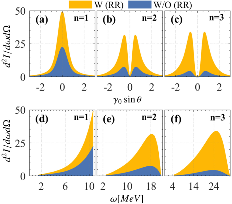
FIG 4: Spatial distributions along direction $\phi=0$ of energy spectra with (W) and without (W/O) RR effects for : (a) first, (b) second, and (c) third harmonics. (d)-(f) similar to (a)-(c) but for the energy dependence. The results are calculated by Eqs. (13) and (14) with $N_{0}=2.4\times 10^{4}$.

To further reveal the RR effects on vortex radiation, the comparison between the absolute spectra without and with RR for each harmonic is shown in Fig. 4. The energy spectra of each harmonic with RR can be enhanced by several times than one without RR. This is because that the modified integrand $J_{n}(p_{c})$and $\mathcal{N}J^{\prime}_{n}(p_{c})$ in Eqs. (13) and (14) have positive contribution to the integration over $\eta$, and thus enhance the radiation field for each harmonic. Moreover, RR can modify the energy allocation among various harmonics, increasing the energy proportion in higher-order harmonics. This is because that RR modifies the intervals between Bessel functions of different orders and their first-order derivatives which are involved as integrands in calculations of radiation field.

IV CONCLUSION

In summary, we investigate the effects of radiation reaction on the production of twisted photons in the nonlinear inverse Thomson scattering. By using Landau-Lifshitz equation, the dominate RR effects on the trajectory of electron are connected to the laser cycles, which indicates that classical radiation reaction effects can be large in long laser pulses while remaining below the threshold for quantum effects. By calculating the Lienard-Wiechert potential using the radiation reaction modified electron trajectory, the vortex field for each harmonic can be obtained. Radiation reaction causes the broadening and even split of resonance function, which implies the center frequency is different from the resonant frequency. The phase structure of vortex field will be modified to the Bessel mode due to radiation reaction. The rotation symmetry of the vortex field and thus the angular momentum in transverse plane can be broken by radiation reaction. Radiation reaction can enhance the energy density of each harmonic and reallocate the proportions of energy on high-order harmonics energy.

V ACKNOWLEDGEMENT

The authors thank M. Katoh for fruitful discussions. The work is supported by the National Natural Science Foundation of China (Grants No. 12022506, No. U2267204, 12105217), the Foundation of Science and Technology on Plasma Physics Laboratory (No. JCKYS2021212008), and the Shaanxi Fundamental Science Research Project for Mathematics and Physics (Grant No. 22JSY014).

Appendix A The concrete derivation of $E_{\theta}$ and $E_{\phi}$

Eq. (7) can be represented in spherical coordinates as:

$$\begin{split}E_{\theta}=&i\sqrt{\frac{e^{2}k^{2}}{32\pi^{3}\varepsilon_{0}^{2}c^{2}}}\frac{e^{ikR}}{R}\int_{-\eta_{00}}^{\eta_{00}}d\eta\\ &(\frac{dx}{d\eta}\cos\theta\cos\phi+\frac{dy}{d\eta}\cos\theta\sin\phi-\frac{dz}{d\eta}\sin\theta)e^{i\psi}\end{split},$$ (23)

$$\begin{split}E_{\phi}=i\sqrt{\frac{e^{2}k^{2}}{32\pi^{3}\varepsilon_{0}^{2}c^{2}}}\frac{e^{ikR}}{R}\int_{-\eta_{00}}^{\eta_{00}}d\eta(\frac{dx}{d\eta}\sin\phi-\frac{dy}{d\eta}\cos\phi)e^{i\psi}\end{split}$$ (24)

Substituting the electron trajectories in Eq (6) into Eqs. (23) and (24), we obtain the integrands in the expressions of $E_{\theta}$ and $E_{\phi}$ separately:

$$\begin{aligned} &\left(\frac{dx}{d\eta}\cos\theta cos\phi+\frac{dy}{d\eta}\cos\theta\sin\phi-\frac{dz}{d\eta}\sin\theta\right)e^{i\psi}\\ &=[k_{0}r_{1}\cos\theta(1+\frac{2}{3}R_{c}k_{0}(\eta-\eta_{0}))\cos\sigma\\ &+\frac{2}{3}R_{c}k_{0}r_{1}\cos\theta(\sin\sigma+\sin\sigma_{0})-\beta_{1}\sin\theta]\cdot\\ &exp\{i[k(\eta-\eta_{0})(1-\beta_{1}(1+\cos\theta))\\ &-p_{c}\sin\sigma-p\frac{2}{3}R_{c}k_{0}(\eta-\eta_{0})\sin\sigma_{0}+\psi_{0}]\}\end{aligned},$$ (25)

$$\begin{aligned} &\left(\frac{dx}{d\eta}sin\phi-\frac{dy}{d\eta}\cos\phi\right)e^{i\psi}\\ &=[-k_{0}r_{1}(1+\frac{2}{3}R_{c}k_{0}(\eta-\eta_{0}))sin\sigma\\ &+\frac{2}{3}R_{c}k_{0}r_{1}(\cos\sigma+\cos\sigma_{0}))]\\ &\cdot exp\{i[k(\eta-\eta_{0})(1-\beta_{1}(1+\cos\theta))\\ &-p_{c}\sin\sigma-p\frac{2}{3}R_{c}k_{0}(\eta-\eta_{0})\sin\sigma_{0}+\psi_{0}]\}\end{aligned}.$$ (26)

Using the following identities, we can expand Eqs. (25) and (26) into series.

$$e^{-ip_{c}\sin\sigma}=\sum_{n=-\infty}^{+\infty}J_{n}(p_{c})e^{-in\sigma},$$ (27a)

$$cos\sigma e^{-ip_{c}\sin\sigma}=\sum_{n=-\infty}^{+\infty}\frac{n}{p_{c}}J_{n}(p_{c})e^{-in\sigma},$$ (27b)

$$sin\sigma e^{-ip_{c}\sin\sigma}=i\sum_{n=-\infty}^{+\infty}J^{\prime}_{n}(p_{c})e^{-in\sigma}$$ (27c)

Finally, we can obtain the series expression for the electric field, namely Eqs (8) and (9).

$$E_{\theta} = \sum_{n=1}^{+\infty}i\sqrt{\frac{e^{2}k^{2}}{32\pi^{3}\varepsilon_{0}^{2}c^{2}}}\frac{e^{ikR+in\phi+i\psi_{0}}}{R}e^{-ink_{0}\eta_{0}}\int_{-\ell_{0}/2}^{\ell_{0}/2}d\eta$$ (28)

$$\times \left\{\left[\frac{nk_{0}\cos\theta}{k\sin\theta}+\frac{2}{3}R_{c}k_{0}r_{1}\sin\sigma-\beta_{1}\sin\theta\right]J_{n}(p_{c})\right.$$

$$+ \left.i\frac{2}{3}R_{c}k_{0}r_{1}J^{\prime}_{n}(p_{c})\right\}e^{-i\bar{k}_{c}(\eta-\eta_{0})}$$

$$,E_{\phi} = \sum_{n=1}^{+\infty}-\sqrt{\frac{e^{2}k^{2}}{32\pi^{3}\varepsilon_{0}^{2}c^{2}}}\frac{e^{ikR+in\phi+i\psi_{0}}}{R}e^{-ink_{0}\eta_{0}}\int_{-\ell_{0}/2}^{\ell_{0}/2}d\eta$$ (29)

$$\times \left\{k_{0}r_{1}\mathcal{N}J^{\prime}_{n}(p_{c})+\frac{2}{3}R_{c}k_{0}r_{1}\frac{n}{p_{c}}J_{n}(p_{c})\right.$$

$$+ \left.\frac{2}{3}R_{c}k_{0}r_{1}\cos\sigma J_{n}(p_{c})\right\}e^{-i\bar{k}_{c}(\eta-\eta_{0})},$$

with $\sigma\equiv k_{0}\eta-\phi$ ($\sigma_{0}=k_{0}\eta_{0}-\phi$) and $\mathcal{N}\equiv\left[1+\frac{2}{3}R_{c}k_{0}(\eta-\eta_{0})\right]$,

Considering $R_{c}\ll 1$, $E_{\theta}$ and $E_{\phi}$ can be approximated as

$$E_{\theta} \simeq \sum_{n}i\sqrt{\frac{e^{2}k^{2}}{32\pi^{3}\varepsilon_{0}^{2}c^{2}}}\frac{e^{ikR+in\phi+i\psi_{0}-ink_{0}\eta_{0}}}{R}\left[\frac{nk_{0}cos\theta}{k\sin\theta}-\beta_{1}\sin\theta\right]$$ (30)

$$\times \int_{-\ell_{0}/2}^{\ell_{0}/2}d\eta J_{n}(p_{c})e^{-i\bar{k}_{c}(\eta-\eta_{0})},$$

$$E_{\phi} \simeq \sum_{n}-\sqrt{\frac{e^{2}k^{2}}{32\pi^{3}\varepsilon_{0}^{2}c^{2}}}\frac{e^{ikR+in\phi+i\psi_{0}-ink_{0}\eta_{0}}}{R}k_{0}r_{1}$$ (31)

$$\times \int_{-\ell_{0}/2}^{\ell_{0}/2}d\eta\mathcal{N}J^{\prime}_{n}(p_{c})e^{-i\bar{k}_{c}(\eta-\eta_{0})}.$$

Substituting the integer-order Bessel function into the above equations and using the following formula

$$\int x^{n}e^{-ikx}dx=-\frac{1}{(ik)^{n+1}}\Gamma(n+1,ikx)+\rm{constant},$$ (32)

$E_{\theta}$ and $E_{\phi}$ can be arranged into the following compact forms

$$E_{\theta} \simeq \sum_{n}iC_{\theta,n}\frac{e^{ikR+in\phi+i\psi_{0}-ink_{0}\eta_{0}}}{R},$$ (33)

$$E_{\phi} \simeq \sum_{n}-C_{\phi,n}\frac{e^{ikR+in\phi+i\psi_{0}-ink_{0}\eta_{0}}}{R}.$$ (34)

The expression of $C_{\theta,n}$ is:

$$C_{\theta,n}= \sqrt{\frac{e^{2}k^{2}}{32\pi^{3}\varepsilon_{0}^{2}c^{2}}}\frac{1}{\frac{2}{3}R_{c}k_{0}p}(\frac{nk_{0}\cos\theta}{k\sin\theta}-\beta_{1}\sin\theta)$$ (35)

$$\sum_{m=0}^{\infty}\frac{(-1)^{m}}{m!(n+m)!}\frac{1}{2^{n+2m}}\frac{1}{(i\tilde{k})^{n+2m+1}}$$

$$(\Gamma(n+2m+1,i\tilde{k}_{c}p)-\Gamma(n+2m+1,i\tilde{k}_{c}p_{m}))$$

The expression of $C_{\phi,n}$ is:

$$C_{\phi,n}= \sqrt{\frac{e^{2}k^{2}}{32\pi^{3}\varepsilon_{0}^{2}c^{2}}}\frac{r_{1}}{\frac{2}{3}R_{c}p^{2}}$$ (36)

$$\sum_{m=0}^{\infty}\frac{(-1)^{m+1}(n+2m)}{m!(n+m)!}\frac{1}{2^{n+2m}}\frac{1}{(i\tilde{k_{c}})^{n+2m+1}}$$

$$(\Gamma(n+2m+1,i\tilde{k}_{c}p)-\Gamma(n+2m+1,i\tilde{k}_{c}p_{m}))$$

Here, $\tilde{k}_{c}={\bar{k}_{c}}{\frac{2}{3}R_{c}k_{0}p}$.

With RR effect, resonance functions are

$$\mathcal{R}_{\theta} =\left|\frac{\int_{-\ell_{0}/2}^{\ell_{0}/2}J_{n}(p_{c})e^{i\bar{k}_{c}(\eta-\eta_{0})}d\eta}{\int_{-\ell_{0}/2}^{\ell_{0}/2}J_{n}(p_{c})d\eta}\right|^{2},$$ (37a)

$$\mathcal{R}_{\phi} =\left|\frac{\int_{-\ell_{0}/2}^{\ell_{0}/2}\mathcal{N}J^{\prime}_{n}(p_{c})e^{i\bar{k}_{c}(\eta-\eta_{0})}d\eta}{\int_{-\ell_{0}/2}^{\ell_{0}/2}\mathcal{N}J^{\prime}_{n}(p_{c})d\eta}\right|^{2},$$ (37b)

for the radiation field along $\theta$ and $\phi$ directions. When $R_{c}=0$, $p_{c}$ is not related to $\eta$, thus resonance functions are:

$$\mathcal{R}_{\theta} =\left|\frac{\int_{-\ell_{0}/2}^{\ell_{0}/2}J_{n}(p_{c})e^{i\bar{k}_{c}(\eta-\eta_{0})}d\eta}{\int_{-\ell_{0}/2}^{\ell_{0}/2}J_{n}(p_{c})d\eta}\right|^{2}$$ (38a)

$$=\left|\frac{\int_{-\ell_{0}/2}^{\ell_{0}/2}e^{i\bar{k}_{c}(\eta-\eta_{0})}d\eta}{\int_{-\ell_{0}/2}^{\ell_{0}/2}d\eta}\right|^{2}=\left|\frac{\sin{(\bar{k}\eta_{0})}}{\bar{k}\eta_{0}}\right|^{2}$$ (38b)

$$\mathcal{R}_{\phi} =\left|\frac{\int_{-\ell_{0}/2}^{\ell_{0}/2}\mathcal{N}J^{\prime}_{n}(p_{c})e^{i\bar{k}_{c}(\eta-\eta_{0})}d\eta}{\int_{-\ell_{0}/2}^{\ell_{0}/2}\mathcal{N}J^{\prime}_{n}(p_{c})d\eta}\right|^{2}$$ (38c)

$$=\left|\frac{\int_{-\ell_{0}/2}^{\ell_{0}/2}e^{i\bar{k}_{c}(\eta-\eta_{0})}d\eta}{\int_{-\ell_{0}/2}^{\ell_{0}/2}d\eta}\right|^{2}=\left|\frac{\sin{(\bar{k}\eta_{0})}}{\bar{k}\eta_{0}}\right|^{2},$$ (38d)

First, we discuss $\mathcal{R}_{\theta}$. For different values of $\bar{k}_{c}$, the denominator of $\mathcal{R}_{\theta}$ is a constant, so the peak of $\mathcal{R}_{\theta}$ depends on the peak of the numerator. When $p_{c}$ does not exceed $\mu_{1}^{(n)}$, $J_{n}(p_{c})$ is always a positive real number, thus the integration factor in the numerator satisfies the following inequality:

$$\left|\int_{-\ell_{0}/2}^{\ell_{0}/2}J_{n}(p_{c})e^{i\bar{k}_{c}(\eta-\eta_{0})}d\eta\right|\leq\int_{-\ell_{0}/2}^{\ell_{0}/2}\left|J_{n}(p_{c})\right|\left|e^{i\bar{k}_{c}(\eta-\eta_{0})}\right|d\eta$$ (39)

$$=\int_{-\ell_{0}/2}^{\ell_{0}/2}\left|J_{n}(p_{c})\right|d\eta=\left|\int_{-\ell_{0}/2}^{\ell_{0}/2}J_{n}(p_{c})e^{i\bar{k}_{c}(\eta-\eta_{0})}d\eta\right|\Big{|}_{\bar{k}_{c}=0}$$

Thus, we know $\mathcal{R}_{\theta}$ has the maximum value at $\bar{k}_{c}=0$.

Similarly, for $R_{\phi}$, there is:

$$\left|\int_{-\ell_{0}/2}^{\ell_{0}/2}\mathcal{N}J^{\prime}_{n}(p_{c})e^{i\bar{k}_{c}(\eta-\eta_{0})}d\eta\right|\leq\int_{-\ell_{0}/2}^{\ell_{0}/2}\left|\mathcal{N}J^{\prime}_{n}(p_{c})\right|\left|e^{i\bar{k}_{c}(\eta-\eta_{0})}\right|d\eta$$ (40)

$$=\int_{-\ell_{0}/2}^{\ell_{0}/2}\left|\mathcal{N}J^{\prime}_{n}(p_{c})\right|d\eta=\left|\int_{-\ell_{0}/2}^{\ell_{0}/2}\mathcal{N}J^{\prime}_{n}(p_{c})e^{i\bar{k}_{c}(\eta-\eta_{0})}d\eta\right|\Big{|}_{\bar{k}_{c}=0}$$

Thus, we know $\mathcal{R}_{\phi}$ has the maximum value at $\bar{k}_{c}=0$.

Appendix B The second-order increments of the electromagnetic field and angular momentum

In the previous calculations, we obtained the first-order increment of the electric field in the frequency domain, denoted as $\bm{E}_{\omega}^{(1)}(\omega,\bm{r})$.The electric field at a specific frequency $\omega$ in the time domain can be expresssed as:

$$\bm{E}^{(1)}(t,\bm{r})=\frac{1}{\sqrt{2\pi}}\bm{E}_{\omega}^{(1)}(\omega,\bm{r})e^{-i\omega t}$$ (41)

From

$$\begin{pmatrix}E^{(1)}_{r}\\ E^{(1)}_{\theta}\\ E^{(1)}_{\phi}\end{pmatrix}=\begin{pmatrix}0\\ \frac{1}{r}\frac{\partial}{\partial r}(rA^{(1)}_{\theta})\\ \frac{1}{r}\frac{\partial}{\partial r}(rA^{(1)}_{\phi})\end{pmatrix}=\begin{pmatrix}0\\ ikA^{(1)}_{\theta}\\ ikA^{(1)}_{\phi},\end{pmatrix},$$ (42)

we can obtain the first-order increment of the vector potential $\bm{A}$. Then, we utilize the following formula to determine the second-order increment of the electromagnetic field:

$$\bm{E^{(2)}}=\begin{pmatrix}E^{(2)}_{r}\\ E^{(2)}_{\theta}\\ E^{(2)}_{\phi}\end{pmatrix}=\begin{pmatrix}-\frac{1}{r\sin\theta}\frac{\partial}{\partial\theta}(\sin\theta A^{(1)}_{\theta})-\frac{1}{r\sin\theta}\frac{\partial}{\partial\phi}A^{(1)}_{\phi}\\ \mathcal{O}\left(\frac{1}{r^{2}}\right)\\ \mathcal{O}\left(\frac{1}{r^{2}}\right)\end{pmatrix},$$ (43)

$$\bm{H^{(2)}}=\begin{pmatrix}H^{(2)}_{r}\\ H^{(2)}_{\theta}\\ H^{(2)}_{\phi}\end{pmatrix}=\begin{pmatrix}\frac{1}{r\sin\theta}\frac{\partial}{\partial\theta}(\sin\theta A^{(1)}_{\phi})-\frac{1}{r\sin\theta}\frac{\partial}{\partial\phi}A^{(1)}_{\theta}\\ \mathcal{O}\left(\frac{1}{r^{2}}\right)\\ \mathcal{O}\left(\frac{1}{r^{2}}\right)\end{pmatrix},$$ (44)

The second-order increments unrelated to angular momentum are not explicitly displayed in Eqs. (43) and (44).

Then, in spherical coordinates, the real part of the time-averaged OAM density of an electromagnetic field $\langle\bm{j}\rangle$ can be expressed as:

$$\langle\bm{j}\rangle\propto\begin{pmatrix}0,&E^{(1)}_{\theta}H^{(2)*}_{r}-H^{(1)*}_{\theta}E^{(2)}_{r},&E^{(1)}_{\phi}H^{(2)*}_{r}-H^{(1)*}_{\phi}E^{(2)}_{r}\end{pmatrix}_{r,\theta,\phi}.$$ (45)

When converted to Cartesian coordinates, angular momentum can be expressed as:

$$\begin{pmatrix}j^{(1)}_{x}\\ j^{(1)}_{y}\\ j^{(1)}_{z}\end{pmatrix}=\begin{pmatrix}-\sin\theta\sin\phi&-\cos\theta\sin\phi&-\cos\phi\\ \sin\theta\cos\phi&\cos\theta\cos\phi&-\sin\phi\\ \cos\theta&-\sin\theta&0\end{pmatrix}\times\begin{pmatrix}0\\ j^{(1)}_{\theta}\\ j^{(1)}_{\phi}\end{pmatrix}.$$ (46)

References

• Bahrdt et al. [2013] J. Bahrdt, K. Holldack, P. Kuske, R. Müller, M. Scheer, and P. Schmid, First Observation of Photons Carrying Orbital Angular Momentum in Undulator Radiation, Phys. Rev. Lett. 111, 034801 (2013).
• Katoh et al. [2017a] M. Katoh, M. Fujimoto, H. Kawaguchi, K. Tsuchiya, K. Ohmi, T. Kaneyasu, Y. Taira, M. Hosaka, A. Mochihashi, and Y. Takashima, Angular Momentum of Twisted Radiation from an Electron in Spiral Motion, Phys. Rev. Lett. 118, 094801 (2017a).
• Katoh et al. [2017b] M. Katoh, M. Fujimoto, N. S. Mirian, T. Konomi, Y. Taira, T. Kaneyasu, M. Hosaka, N. Yamamoto, A. Mochihashi, Y. Takashima, K. Kuroda, A. Miyamoto, K. Miyamoto, and S. Sasaki, Helical Phase Structure of Radiation from an Electron in Circular Motion, Sci. Rep. 7, 6130 (2017b).
• Taira et al. [2017] Y. Taira, T. Hayakawa, and M. Katoh, Gamma-ray vortices from nonlinear inverse Thomson scattering of circularly polarized light, Sci. Rep. 7, 5018 (2017).
• Chen et al. [2019] Y.-Y. Chen, K. Z. Hatsagortsyan, and C. H. Keitel, Generation of twisted $\gamma$ -ray radiation by nonlinear Thomson scattering of twisted light, Matter Radiat. Extremes 4, 024401 (2019).
• Torres and Torner [2011] J. P. Torres and L. Torner, Twisted photons: applications of light with orbital angular momentum (John Wiley & Sons, 2011).
• Molina-Terriza et al. [2007] G. Molina-Terriza, J. P. Torres, and L. Torner, Twisted photons, Nat. Phys. 3, 305 (2007).
• van Veenendaal and McNulty [2007] M. van Veenendaal and I. McNulty, Prediction of strong dichroism induced by x rays carrying orbital momentum, Phys. Rev. Lett. 98, 157401 (2007).
• Erhard et al. [2018] M. Erhard, R. Fickler, M. Krenn, and A. Zeilinger, Twisted photons: new quantum perspectives in high dimensions, Light: Science & Applications 7, 17146 (2018).
• Harwit [2003] M. Harwit, Photon orbital angular momentum in astrophysics, Astrophys. J. 597, 1266 (2003).
• II [2008] N. E. II, Photon orbital angular momentum in astronomy, Astron. Astrophys. 492, 883 (2008).
• Blackburn [2020] T. G. Blackburn, Radiation reaction in electron–beam interactions with high-intensity lasers, Rev. Mod. Plasma Phys. 4, 5 (2020).
• Gonoskov et al. [2022] A. Gonoskov, T. G. Blackburn, M. Marklund, and S. S. Bulanov, Charged particle motion and radiation in strong electromagnetic fields, Rev. Mod. Phys. 94, 045001 (2022).
• Sun et al. [2022] T. Sun, Q. Zhao, K. Xue, Z.-W. Lu, L.-L. Ji, F. Wan, Y. Wang, Y. I. Salamin, and J.-X. Li, Production of polarized particle beams via ultraintense laser pulses, Rev. Mod. Plasma Phys. 6, 38 (2022).
• Fedotov et al. [2023] A. Fedotov, A. Ilderton, F. Karbstein, B. King, D. Seipt, H. Taya, and G. Torgrimsson, Advances in QED with intense background fields, Phys. Rep. 1010, 1 (2023).
• Landau [2013] L. D. Landau, The classical theory of fields, Vol. 2 (Elsevier, 2013).
• Di Piazza and Audagnotto [2021] A. Di Piazza and G. Audagnotto, Analytical spectrum of nonlinear Thomson scattering including radiation reaction, Phys. Rev. D 104, 016007 (2021).
• Li et al. [2014] J.-X. Li, K. Z. Hatsagortsyan, and C. H. Keitel, Robust Signatures of Quantum Radiation Reaction in Focused Ultrashort Laser Pulses, Phys. Rev. Lett. 113, 044801 (2014).
• Li et al. [2018] J.-X. Li, Y.-Y. Chen, K. Z. Hatsagortsyan, and C. H. Keitel, Single-Shot Carrier-Envelope Phase Determination of Long Superintense Laser Pulses, Phys. Rev. Lett. 120, 124803 (2018).
• Guo et al. [2020] R.-T. Guo, Y. Wang, R. Shaisultanov, F. Wan, Z.-F. Xu, Y.-Y. Chen, K. Z. Hatsagortsyan, and J.-X. Li, Stochasticity in radiative polarization of ultrarelativistic electrons in an ultrastrong laser pulse, Phys. Rev. Research 2, 033483 (2020).
• Di Piazza [2008] A. Di Piazza, Exact Solution of the Landau-Lifshitz Equation in a Plane Wave, Lett. Math. Phys. 83, 305 (2008).
• Di Piazza [2018] A. Di Piazza, Analytical infrared limit of nonlinear Thomson scattering including radiation reaction, Physics Letters B 782, 559 (2018).
• Esarey et al. [1993] E. Esarey, S. K. Ride, and P. Sprangle, Nonlinear Thomson scattering of intense laser pulses from beams and plasmas, Phys. Rev. E 48, 3003 (1993).