Correspondences of the Third Kind:
Camera Pose Estimation from Object Reflection

Abstract

Computer vision has long relied on two kinds of correspondences: pixel correspondences in images and 3D correspondences on object surfaces. Is there another kind, and if there is, what can they do for us? In this paper, we introduce correspondences of the third kind we call reflection correspondences and show that they can help estimate camera pose by just looking at objects without relying on the background. Reflection correspondences are point correspondences in the reflected world, i.e., the scene reflected by the object surface. The object geometry and reflectance alters the scene geometrically and radiometrically, respectively, causing incorrect pixel correspondences. Geometry recovered from each image is also hampered by distortions, namely generalized bas-relief ambiguity, leading to erroneous 3D correspondences. We show that reflection correspondences can resolve the ambiguities arising from these distortions. We introduce a neural correspondence estimator and a RANSAC algorithm that fully leverages all three kinds of correspondences for robust and accurate joint camera pose and object shape estimation just from the object appearance. The method expands the horizon of numerous downstream tasks, including camera pose estimation for appearance modeling (e.g., NeRF) and motion estimation of reflective objects (e.g., cars on the road), to name a few, as it relieves the requirement of overlapping background.

1 Introduction

Look at the two images in Fig. 1. Even for this extreme case of a perfect mirror object, we—as humans—can understand how the camera moved (at least qualitatively) between the two images. This likely owes to our ability to disentangle the reflected surroundings from surface appearance.

How would a computer estimate the camera pose change between the two images? Structure-from-motion would fail in such conditions because they rely on pixel correspondences, i.e., matched projections of the same physical surface points in the images, which would be erroneous as the glossy reflection violates the color constancy constraint.

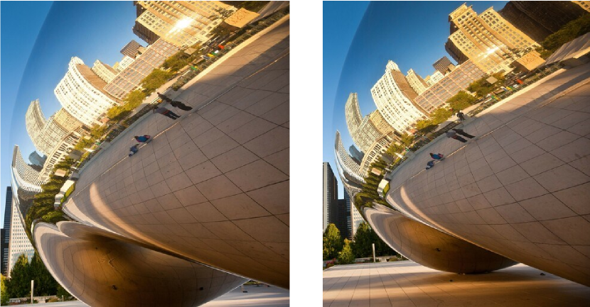
Figure 1: We humans can tell how the camera moved between the images, but computers have a hard time. Can we estimate camera pose and possibly object shape just from object appearance, despite the featureless appearance and non-overlapping background? (Photos by Richard Ellis/Alamy)

Recent neural shape-from-shading methods can recover the object geometry as surface normals in each view even under complex natural illumination [21]. As the illumination is unknown, the recovered surface normals, however, suffer from a fundamental ambiguity known as the generalized bas-relief ambiguity [1] between light source and surface geometry. That is, a rotated illumination and sheered surface can conspire to generate the exact same object appearance. As such, 3D correspondences established between the two surface normal maps recovered independently from the two images would only tell us the camera pose in the distorted space.

In fact, we show that even if we use both pixel correspondences in the images and 3D correspondences on the recovered object surfaces, we cannot resolve this ambiguity for orthographic cameras. Even with a perspective camera, the object is often far enough that this limitation still holds. Even if we have more than two views, joint estimation of the camera poses and the object shape with the erroneous normal maps would be still challenging. The geometry estimate can easily fall into local minima whose surface normals (i.e., local surface geometry) are consistent with the current camera pose estimates.

How then can camera pose be estimated just from the object appearance? We take a hint from what we humans likely do: establish correspondences in the world reflected by the object surface. By leveraging the single-view reconstruction of surface normals, we can extract from each of the images a reflectance map. The reflectance map is the Gaussian sphere of the reflected radiance. It represents the surrounding environment modulated by surface reflectance as a spherical surface indexed by surface normals. We establish correspondences between the reflectance maps of the images. We refer to these as reflection correspondences.

We show that these reflection correspondences by themselves are not sufficient to directly compute the camera pose. They, however, resolve the ambiguity remaining in the point and 3D correspondences in presence of the bas-relief ambiguity. This means that, by using all three types of correspondences in two or more images of an object of arbitrary reflectance, even without any texture and with strong specularity, we can compute the relative camera poses just from the object appearances. This liberates many applications from seemingly benign yet practically extremely limiting requirement of overlapping static background or diffuse surface texture just to recover camera positions.

We formalize reflection correspondences and show how they should be combined with conventional correspondences (pixel correspondences and 3D correspondences) to obtain a quantitative estimate of the correct camera rotation. We also introduce a new neural feature extractor for establishing 3D and reflection correspondences robust to the inherent distortions primarily caused by the bas-relief ambiguity with effective data augmentation. Finally, we derive a RANSAC-based joint estimation framework for accurate joint camera pose and geometry reconstruction which alternates between the interdependent two quantities.

Experimental results on synthetic correspondences and images show that the reflection correspondences and the neural feature extractor as well as our iterative estimation framework are essential for accurate camera pose and geometry estimation. We believe reflection correspondences can play an important role in applications beyond camera pose and shape recovery from object appearance, including camera calibration [2] and object pose estimation [14] when classical correspondences are not sufficient.

2 Related Work

In this paper, we address camera pose estimation from a small number (2) of views of textureless, non-Lambertian (e.g., shiny) objects taken under unknown natural illumination, which remains challenging for existing methods especially when good initial estimates are not available.

Structure-from-motion methods recover camera poses for multiple images by detecting and leveraging pixel correspondences [25, 16]. They typically detect such pixel correspondences by leveraging view-independent, salient features such as textures and jointly solve for camera poses and 3D locations of the surface points. Descriptors invariant to rotation and scale (e.g., SIFT [10]) and outlier correspondence detection with RANSAC [5] are often exploited for robust estimation. However, these methods are prone to fail on textureless, non-Lambertian objects (especially, shiny objects) as correspondences between surface points are extremely challenging to establish on these objects. Also, correspondences based on textures are usually sparse, and these methods require a large number (e.g., 50) of input images that have high visual overlaps for accurate estimation.

Neural image synthesis methods jointly estimate surface geometry and a surface light field (or its radiometric roots, i.e., reflectance and illumination) as neural representations with differentiable volumetric [11, 13, 24, 19, 9] or surface [22, 23] rendering. While most of these methods require multiple registered images as inputs, a few methods also handle non-registered multi-view images by optimizing the camera poses as additional parameters [22, 3]. They, however, still require good initial estimates of camera poses (e.g., SAMURAI [3] uses manually annotated coarse camera poses as inputs) or an extremely large number ($>$50) of input images as the joint optimization of all unknown parameters is extremely challenging and easily falls into local minima.

Pose estimation from specular reflections has also been studied [8, 15, 4, 12]. Lagger et al. [8], for instance, refine camera pose estimates using images and the 3D CAD model of a specular object. They recover view-dependent environment maps from the inputs and optimize the camera pose by minimizing discrepancies between them. These methods, however, assume known geometry [8, 15, 4, 12], known illumination [4], or a simple lighting model (i.e., directional or point source) [15, 12] which cannot be assumed in general scenes.

In contrast, reflection correspondences enable us to recover the camera pose and object geometry of arbitrary objects under complex natural illumination without requiring static overlapping background to be present in the image.

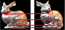
(a) Pixel Correspondences

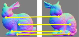
(b) 3D Correspondences

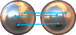
(c) Reflection Correspondences

Figure 2: We show how to leverage three types of correspondences. Pixel correspondences (a) are the pixels that correspond to the same surface point. We can also leverage similar correspondences in the normal maps which we refer to as 3D correspondences (b). In addition to these correspondences, we leverage novel correspondences about the surrounding environment which we can observe through surface reflection. We recover camera-view reflectance maps, maps that associate surface normal orientations with the surrounding environment, and detect this type of correspondences from them (c). We refer to this novel kind of correspondences as reflection correspondences.

3 Method

In this section, we first detail the three types of correspondences we consider and the equations that can be derived from them. Figure 2 provides a visualization of these three types of correspondences. To avoid confusion, we refer to them by the following names:

• “pixel correspondences”, for the “classical correspondences” which link corresponding locations in the two images on the object surface: the two matched points are the reprojections of the same physical 3D point in the two images.

• “3D correspondences”, for the correspondences between corresponding normals in the two images on the object surface. Note that for each pixel correspondence, we also have a 3D correspondence if we know the normals at the matched image locations. The difference is that for the pixel correspondence, we exploit the pixel coordinates themselves, while in the case of the 3D correspondence, we exploit the normals.

• “reflection correspondences”, which match image locations where light rays creating specular reflections come from the same direction in the two images. As shown in Fig. 2(c), we detect these correspondences from camera-view reflectance maps, i.e., view-dependent maps about the surrounding environment.

In this paper, we assume orthographic projection as objects are usually distant from the cameras and we can regard camera rays that point at the object as almost constant. Note that, as we see in the next subsection, camera pose estimation is challenging especially under orthographic projection.

3.1 Pixel Correspondences

Let us assume that we can establish $N_{\mathrm{IM}}$ pixel correspondences $(u_{1}^{i},v_{1}^{i})\leftrightarrow(u_{2}^{i},v_{2}^{i})$. Under orthographic projection, each pixel correspondence gives us one constraint on the camera rotation between the two images [6]:

$$\left[(u_{1}^{i}\cos\phi+v_{1}^{i}\sin\phi)-(u_{2}^{i}\cos\theta+v_{2}^{i}\sin\theta)\right]^{2}=0\,,$$ (1)

where $\phi$ and $\theta$ are two of three Euler angles $(\theta,\phi,\eta)$ that correspond to the relative rotation $\mathrm{R_{21}}$ from the second view to the first one. Without loss of generality, we assume that these correspondences are shifted such that the average location (e.g., $\frac{1}{N_{\mathrm{IM}}}\sum_{i}u_{1}^{i}$) is zero. We use the (z-x-z) sequence for the Euler angles

$$\mathrm{R_{21}}=\mathrm{R_{z}}[\phi]~{}\mathrm{R_{x}}[\eta]~{}\mathrm{R_{z}}[-\theta]\,,$$ (2)

where $\mathrm{R_{z}}[\cdot]$ and $\mathrm{R_{x}}[\cdot]$ are rotations around z and x axes, respectively. Since Eq. 1 is independent of one of the unknown Euler angles ($\eta$), it is not possible to fully recover the rotation matrix from pixel correspondences when we have only two views.

3.2 3D Correspondences

If we could estimate unambiguously the normal maps ${\bf N}_{1}$ and ${\bf N}_{2}$ for the images, correspondences $(u_{1}^{i},v_{1}^{i})\leftrightarrow(u_{2}^{i},v_{2}^{i})$ would be constrained by

$${\bf N}_{1}[u_{1}^{i},v_{1}^{i}]=\mathrm{R_{21}}{\bf N}_{2}[u_{2}^{i},v_{2}^{i}]\,,$$ (3)

as the normals at locations $(u_{1}^{i},v_{1}^{i})$ and $(u_{2}^{i},v_{2}^{i})$ are the same up to rotation $\mathrm{R}_{21}$. We then could estimate the relative rotation $\mathrm{R}_{21}$ by simply solving Eq. 3.

Unfortunately, in practice, normal maps can be recovered only up to the generalized bas-relief (GBR) ambiguity [1]. Given a normal map $\mathbf{N}$ for an image $I$, any normal map ${\bf N}^{\prime}$ with

$${\bf N}^{\prime}[u,v]=\mathrm{G}^{-\mathrm{T}}{\bf N}[u,v]\,,$$ (4)

could result in the same image $I$ under a different lighting, where $\mathrm{G}$ is the generalized bas-relief (GBR) transformation [1]

$$\mathrm{G}\equiv\begin{pmatrix}1&0&0\\ 0&1&0\\ \mu&\nu&\lambda\end{pmatrix}\,.$$ (5)

$\mu$ and $\nu$ can take any values, and $\lambda$ can take any positive value. Note that, while discussions regarding the bas-relief ambiguity (e.g., one in Belhumeur et al. [1]) usually assume directional lights, this holds true even for environmental illumination as we can see it as a set of directional lights.

The bas-relief ambiguity changes the relationship in Eq. 3 to

$${\bf N}_{1}[u_{1}^{i},v_{1}^{i}]\propto\mathrm{G_{1}}^{-\mathrm{T}}\mathrm{R_{21}}\mathrm{G_{2}}^{\mathrm{T}}{\bf N}_{2}[u_{2}^{i},v_{2}^{i}]\,,$$ (6)

where $\mathrm{G_{k}}$ $(k=1,2)$ is an unknown GBR transformation for each view that corresponds to the estimation errors [1]. If we have a sufficient number of correspondences, we can obtain a unique solution for the combined transformation

$$\mathrm{G}_{21}\equiv\mathrm{G_{1}}^{-\mathrm{T}}\mathrm{R_{21}}\mathrm{G_{2}}^{\mathrm{T}}\,.$$ (7)

There is, however, an unresolvable ambiguity in its decomposition into the three unknown matrices. Most important, this ambiguity corresponds to one regarding the pixel correspondences, in other words, we cannot recover the relative camera pose even when combining pixel and 3D correspondences: for any $\eta$, there are corresponding GBR transformations $\mathrm{G_{1}}$ and $\mathrm{G_{2}}$ that are consistent with Eq. 6. We provide the proof in the supplementary material.

3.3 Reflection Correspondences

Let us assume we have correspondences between image locations $(u_{1}^{i},v_{1}^{i})\leftrightarrow(u_{2}^{i},v_{2}^{i})$ where light rays come from the same direction in the two images. In other words, correspondences of the surroundings reflected by the object surface. If we, for now, ignore the GBR ambiguity, these “reflection” correspondences give each a constraint of the form

$$\omega_{\mathrm{r}}({\bf N}_{1}[u_{1}^{i},v_{1}^{i}])\propto\mathrm{R_{21}}\omega_{\mathrm{r}}({\bf N}_{2}[u_{2}^{i},v_{2}^{i}])\,,$$ (8)

where function $\omega_{\mathrm{r}}({\bf n})$ returns the reflection of the line of sight direction $\omega_{o}$ on the surface with normal ${\bf N}$:

$$\omega_{\mathrm{r}}({\bf n})=-\omega_{o}+2\frac{\omega_{o}\cdot{\bf n}}{{\bf n}\cdot{\bf n}}{\bf n}\,.$$ (9)

Again, at this stage, we can in fact predict the normal maps only up to the GBR ambiguity, and we need to introduce the two GBR transformations into Eq. 8:

$$\omega_{\mathrm{r}}(\mathrm{G_{1}}^{\mathrm{T}}{\bf N}_{1}[u_{1}^{i},v_{1}^{i}])\propto\mathrm{R_{21}}\omega_{\mathrm{r}}(\mathrm{G_{2}}^{\mathrm{T}}{\bf N}_{2}[u_{2}^{i},v_{2}^{i}])\,.$$ (10)

Each reflection correspondence thus gives us a new type of equations to estimate $\mathrm{R_{21}}$ but also $\mathrm{G_{1}}$ and $\mathrm{G_{2}}$, from which we can also get the object shape.

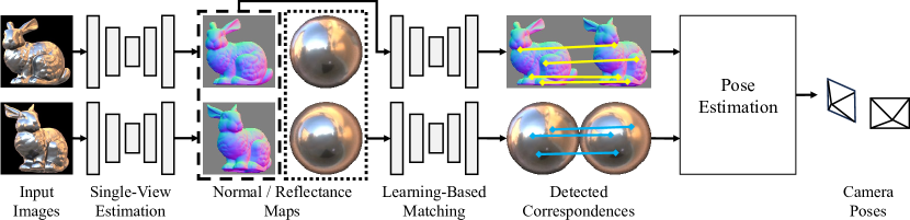
Figure 3: Given two-view images of a textureless, non-Lambertian object, we first recover surface normals and reflectance map for each view using a single-view geometry reconstruction method [21]. We establish 3D and reflection correspondences with a novel deep feature extraction network (Fig. 5) to compute the relative camera pose from them.

Detection of these reflection correspondences directly from images is, however, extremely challenging as surface reflection depends not only on the surrounding illumination but also on the surface geometry. Let us now assume we have a surface normal map for each view. Then we can avoid this problem by recovering camera-view reflectance maps [7]. The reflectance maps are view-dependent mappings from a surface normal to the surface radiance which are determined by the surface reflectance and the surrounding illumination environment

$$E_{k}(\mathbf{n})=\int L_{i}(\mathrm{R}_{k}^{\mathrm{T}}\mathbf{\omega_{i}})\psi(\mathbf{\omega_{i}},\mathbf{\omega_{o}},\mathbf{n})\max(\mathbf{\omega_{i}}\cdot\mathbf{n},0)\mathrm{d}\mathbf{\omega_{i}}\,,$$ (11)

where $\mathbf{\omega_{i}}$, $\mathbf{\omega_{o}}$, $\mathbf{n}$ are incident, viewing, and surface normal orientations in the local camera coordinate system, respectively. $\mathrm{R}_{k}$ is the camera pose (a rotation matrix) of $k$-th view, $L_{i}(\mathrm{v})$ is a mapping from an incident direction to a radiance of the the corresponding incident light, and $\psi(\mathbf{\omega_{i}},\mathbf{\omega_{o}},\mathbf{n})$ is the bidirectional reflectance distribution function (BRDF).

From the surface normal maps and the input images, i.e., pairs of surface normals and surface radiances, we can recover these reflectance maps and, as illustrated in Fig. 2(c), detect these reflection correspondences from the reflectance maps regardless of the object shape. Note that, as the reflectance maps are recovered using the surface normal maps, they also suffer from the bas-relief ambiguity. The relationship between the ground truth $E(\mathbf{n})$ and another possible solution $E(\mathbf{n})$ is

$$E^{\prime}(\mathbf{n})=E(\mathrm{G}^{\mathrm{T}}\mathbf{n})\,.$$ (12)

Thus we still need to use Eq. 10 for these reflection correspondences.

3.4 Objective Function

From Eq. 1, (6), and (10), we derive the objective function

$$f=f_{\text{IM}}+f_{\text{NM}}^{(12)}+f_{\text{NM}}^{(21)}+f_{\text{RM}}^{(12)}+f_{\text{RM}}^{(21)}\,.$$ (13)

that enforces the equation in the least-squares sense. $f_{\text{IM}}$ enforces Eq. 1:

$$f_{\text{IM}}=\sum_{i}^{N_{\text{IM}}}\left(t_{\phi}^{i}-t_{\theta}^{i}\right)^{2}\,,$$ (14)

with

$$t_{\phi}^{i}=u_{1}^{i}\cos\phi+v_{1}^{i}\sin\phi\,,$$ (15)

$$t_{\theta}^{i}=u_{2}^{i}\cos\theta+v_{2}^{(i)}\sin\theta\,,$$ (16)

and $N_{\text{IM}}$ is the number of image correspondences.

Note that for Eq. 6 and Eq. 10, we can switch the role of the two images. We therefore introduce two terms for each of these equations. For Eq. 6, we introduce

$$f_{\text{NM}}^{(jk)}=\sum_{i}^{N_{\text{NM}}}\left\|{\bf N}_{j}[u_{j}^{i},v_{j}^{i}]-{\text{Norm}}(\mathrm{G}_{kj}{\bf N}_{k}[u_{k}^{i},v_{k}^{i}])\right\|^{2}\,,$$ (17)

where Norm is the vector normalization operator and $N_{\text{NM}}$ the number of 3D correspondences.

For Eq. 10, we introduce

$$f_{\text{RM}}^{(jk)}=\sum_{i}^{N_{\text{RM}}}\left\|{\bf N}_{j}[u_{j}^{i},v_{j}^{i}]-\Omega^{(jk)}({\bf N}_{k}[u_{k}^{i},v_{k}^{i}])\right\|^{2}\,,$$ (18)

where $\Omega^{(jk)}({\bf n})$ transforms a surface normal ${\bf n}$ in the $j$-th view reflectance map to the surface normal in the $k$-th view

$$\Omega^{(jk)}({\bf n})={\text{Norm}}(\mathrm{G}_{k}^{-T}\omega_{\mathrm{r}}^{-1}(\mathrm{R}_{jk}\;\omega_{\mathrm{r}}(\mathrm{G}_{j}^{T}{\bf n})))\,.$$ (19)

Given 3 sets of $N_{\text{IM}}$ pixel correspondences, $N_{\text{NM}}$ 3D correspondences, and $N_{\text{RM}}$ reflection correspondences, we optimize $f$ in Eq. 13 for the three Euler angles $\theta$, $\phi$, and $\eta$, and the two sets of parameters for the GBR transformations for both images $\mu_{1}$, $\nu_{1}$, $\lambda_{1}$, $\mu_{2}$, $\nu_{2}$, $\lambda_{2}$, under the constraints that $\lambda_{1}$ and $\lambda_{2}$ are positive. We empirically find that naive nonlinear optimization with all the correspondences is slow and susceptible to local minima. We instead derive a two-step algorithm that first estimates the combined transformation $\mathrm{G_{21}}$ using pixel and 3D correspondences and then decomposes it using reflection correspondences. Nonlinear optimization with an off-the shelf solver [18] is used for the first step. In the second step, we discretize $\eta$ in 180 angles, solve for the other parameters analytically, and check if the obtained parameters are consistent with reflectance map correspondences. The supplementary material provides more details.

Intuition on the required numbers of correspondences.

In practice, the numbers of correspondences required for the camera pose estimation is important as we can use them for a robust estimation with RANSAC [5]. Although it is difficult to derive a rigorous proof about the number of required correspondences, we can build intuition about how many correspondences are required for each view pair. We first consider estimation from 3D correspondences in normal maps. Each correspondence gives us 1 constraint from the images and 2 from the normal maps—only 2 because, while the surface normals are 3-vectors, they are normalized. The number of unknown parameters except for the unresolvable parameter $\eta$ is 8. Thus the expected number of required 3D correspondences in normal maps is 3. One reflection correspondence is also required for resolving the remaining ambiguity about $\eta$. We indeed experimentally confirmed that three 3D and one reflection correspondences used together for direct optimization of all transformations ($\mathrm{G_{1}},\mathrm{G_{2}}$ and $R_{21}$) are sufficient. When using the sequential two-step algorithm, however, we empirically find in Sec. 4.1 that we need four 3D correspondences instead of three for the first stage of estimating the combined transformation $\mathrm{G_{21}}$. This is actually consistent with the total of 4 mixed 3D and reflection correspondences necessary for a direct optimization, likely suggesting that the least-square estimation of the combined transformation always needs at least a total of four correspondences of whatever form. Deriving a rigorous theoretical understanding of this would open new interesting research directions in 3D geometry.

3.5 Camera Pose Estimation from Two Images

Figure 3 depicts how the camera pose between two views can be recovered. To recover the normal maps ${\bf N}_{1}$ and ${\bf N}_{2}$, we use DeepShaRM which is a radiometry-based geometry estimation method [21] to each input image independently. This gives us the normal maps but only up to the GBR transformations. DeepShaRM also recovers a reflectance map for each view from the normal maps. We use these outputs for the reflection correspondence detection.

To obtain 3D correspondences in the normal maps, we train a deep network to extract pixel-wise, view-invariant features that we use to match locations across the normal maps. Figure 5 depicts this feature extraction network. We train the network by contrastive learning. We use pairs of synthetic normal maps of two views as training data. We feed both of them to the feature extraction network and obtain corresponding feature maps ${\bf F}_{1}$ and ${\bf F}_{2}$. Given ground truth correspondences $(u_{1}^{i},v_{1}^{i})\leftrightarrow(u_{2}^{i},v_{2}^{i})$, we impose the InfoNCE loss [17]

$$L=\sum_{i}\sum_{j}-\delta_{ij}\log\left(\frac{\exp(c_{ij})}{\sum_{i^{\prime}}\sum_{j^{\prime}}\exp(c_{i^{\prime}j^{\prime}})}\right)\,,$$ (20)

where $c_{ij}$ is the cosine similarity of feature vectors ${\bf F}_{1}[u_{1}^{i},v_{1}^{i}]$ and ${\bf F}_{2}[u_{2}^{j},v_{2}^{j}]$

$$c_{ij}={\text{Norm}}({\bf F}_{1}[u_{1}^{i},v_{1}^{i}])\cdot{\text{Norm}}({\bf F}_{2}[u_{2}^{j},v_{2}^{j}])\,,$$ (21)

and $\delta_{ij}$ is the Kronecker delta. By this, we ensure that features of pixels that correspond to the same surface point become similar.

The training with synthetic normal maps is, however, insufficient for 3D correspondence detection in the estimated normal maps as they are distorted by GBR transform. We overcome this with data augmentation. For each view in the training data, we randomly sample parameters of the GBR transformation and transform the input normal map according to Eq. 4. We use the transformed normal maps instead of the original ones so that the network can learn to extract features robust to the estimation errors caused by the bas-relief ambiguity.

At inference time, using the extracted feature maps, we detect correspondences by brute-force matching and filter them with the ratio test by Lowe [10]. For any location on the object in the first image, we look for the best and second best locations in the second image in terms of the cosine similarity of the features. If the ratio of the similarity of the second best location to one of the best location is lower than a threshold, we use the best location as the matched location. This gives us both pixel correspondences and 3D correspondences.

We also train another deep neural network reflection correspondences in the same way. Please see the supplementary for more details.

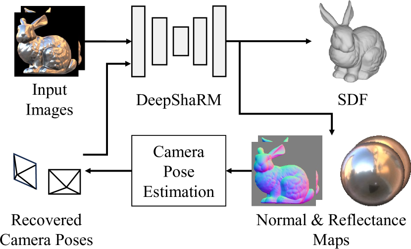
Figure 4: Once we recover the camera poses, we can iteratively refine them by alternating between estimation of the surface normals and reflectance maps, and the camera poses. We use DeepShaRM [21] to update the normals and reflectance maps. DeepShaRM also outputs a unified surface geometry estimate as a 3D grid of a singled distance function (SDF).

Once we have the three types of correspondences, we recover the relative rotation using our two-step algorithm (Sec. 3.4). For robust estimation, we perform the first step with RANSAC [5]. We estimate different candidates of the combined transformation $\mathrm{G_{21}}$ from randomly sampled minimal sets of pixel and 3D correspondences. We then select one of them according to the number of inlier correspondences, i.e., ones that are consistent with the estimated parameters. In the second step, for each possible decomposition of $\mathrm{G_{21}}$, we check the number of inlier reflection correspondences that are consistent with the decomposed parameters and select one according to it. Based on Sec. 4.1, we use four pixel and four 3D correspondences from the normal map pair as the minimal set for the estimation in the first step.

3.5.1 Translation Estimation

Once $\mathrm{R_{21}}$ is determined, by leveraging the pixel correspondences, we can also solve for the relative translation between the two views except for offsets regarding the two viewing directions [6]. That is, we estimate the translation vector $\mathbf{t_{21}}=(t_{x},t_{y},t_{z})$ using the constraint

$$r_{23}t_{x}-R_{13}t_{y}=-\sum_{i}\left(r_{23}\tilde{u}^{i}-r_{13}\tilde{v}^{i}\right)\,,$$ (22)

where $r_{jk}$ is $(j,k)$ element of $\mathrm{R_{21}}$ and

$$\tilde{u}^{i}=r_{11}u_{2}^{i}+r_{12}v_{2}^{i}-u_{1}^{i}\,,$$ (23)

$$\tilde{v}^{i}=r_{21}u_{2}^{i}+r_{22}v_{2}^{i}-v_{1}^{i}\,.$$ (24)

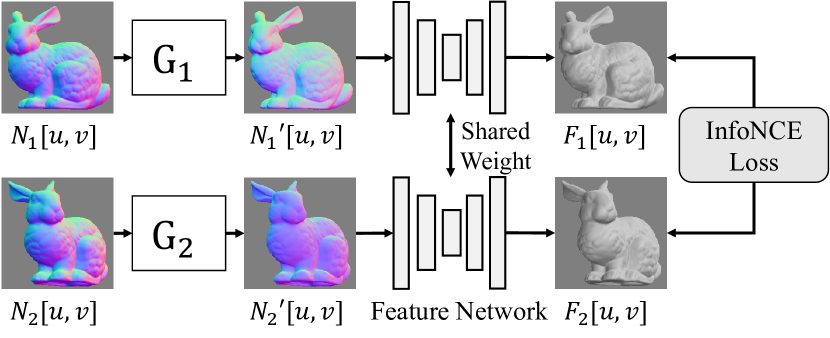
Figure 5: We train a deep neural network to extract view-independent, per-pixel features for correspondence matching. Contrastive learning using InfoNCE loss [17] with data augmentation with the GBR transform enables feature extraction for distortion-robust correspondence matching.

3.6 Joint Shape and Camera Pose Recovery

As depicted in Fig. 4, we further improve the camera pose estimation accuracy by alternating between estimating camera poses using the surface normal and reflectance map estimates and updating them using the camera pose estimates. As a byproduct, we obtain an accurate object shape. For the update of the surface normal and reflectance map estimates, we use DeepShaRM [21]. Using the camera poses as inputs, DeepShaRM integrates the multi-view estimates of surface normals and output improved estimates along with a surface geometry estimate represented as a 3D signed distance function.

If we have more than two views, we can integrate the estimated relative camera pose for each view pair. We first initialize a camera pose estimate for each view $\mathrm{R_{k}}$ using some of the recovered relative poses. Using inlier correspondences, we then refine the pose estimates by minimizing the sum of the objective functions from Eq. 13 over each view pair.

4 Experimental Results

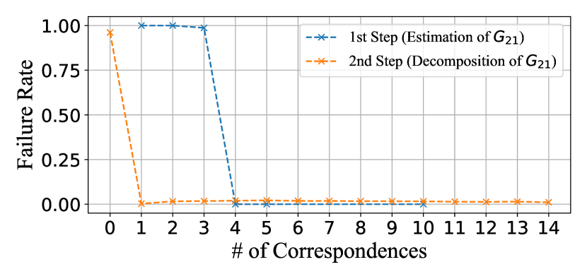
Figure 6: Empirical analysis of the number of correspondences required for optimization of the camera pose and the two GBR transforms of two images. See text for details.

	Pose Error
w/o Data Augm.	13.4 deg
w/o Joint	7.1 deg
Ours	6.1 deg

Table 1: Camera pose estimation accuracy on images in the nLMVS-Synth dataset [20]. Please see the text for details.

We focus our experiments on answering the following key questions. What are the actual number of correspondences required for resolving the bas-relief ambiguity? Can the novel feature extraction network establish correspondences robust to GBR distortion? To answer these questions, we validate the following points

• The intuition about the number of required correspondences is consistent with results of empirical evaluation.

• The proposed components (e.g., the data augmentation) are essential for accurate reconstruction from a sparse set (2) of images.

4.1 The Number of Correspondences

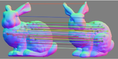
(a) 3D Correspondences

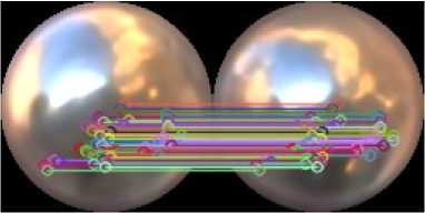
(b) Reflection Correspondences

Figure 7: Examples of 3D and reflection correspondences detected by our method. Visual inspection shows that they match semantically correct surface and reflectance map points.

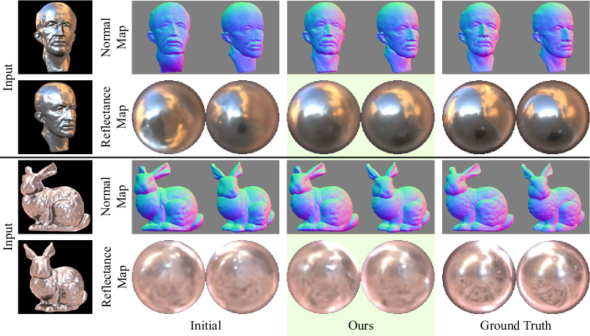
Figure 8: Surface normal and reflectance maps recovered from two synthetic images in the nLMVS-Synth dataset. The bas-relief ambiguity is successfully resolved and the recovered maps are consistent with ground truth.

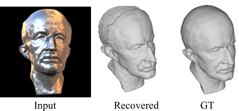
Figure 9: Surface geometry recovered by the joint estimation.

We first conduct empirical evaluation of the number of correspondences required for resolving the bas-relief ambiguity for each view pair. We created 10000 sets of synthetic correspondences by randomly sampling surface normal orientations, relative rotation matrices, and parameters of the GBR transformation. Using this synthetic data, we checked how the numbers of correspondences used for the two-step algorithm (Sec. 3.4) affects the estimation accuracy. In this experiment, we optimized all the unknown parameters with all available correspondences using an off-the-shelf solver [18] as the two step algorithm cannot be applied to cases where reflection correspondences are not available. In the following results, we exclude cases where the objective function did not converge to zero as it is a symptom that the optimization algorithm did not converge correctly.

The blue line in Fig. 6 shows the relationship between the number of correspondences in normal maps (pixel and 3D correspondences) and rate of failure cases where the error (Frobenius norm) between estimated combined transformation matrix $\mathrm{G_{21}}$ and the ground truth is higher than 0.01. To simulate the first step of the algorithm, we did not use reflection correspondences in this experiment. The results show that four correspondences are required for the estimation of $\mathrm{G_{21}}$. The orange line in Fig. 6 shows the relationship between the number of reflection correspondences and rate of failure cases where the error between the estimated camera pose and the ground truth is higher than 0.1 degree. In this experiment, we used four pixel and four 3D correspondences in addition to the reflection correspondences. The results show that one reflection correspondence resolves the remaining ambiguity. Note that, the leftmost point in the orange line shows that, without reflection correspondences, we cannot decompose the combined transformation $\mathrm{G_{21}}$. These results are consistent with the intuition discussed in Sec. 3.4.

4.2 Camera Pose Estimation

We evaluate the accuracy of the joint camera pose and object shape estimation framework on synthetic images. We train the feature extraction network using synthetic normal and reflectance maps on the nLMVS-Synth dataset [20].

For quantitative evaluation, we test our method on synthetic images from the test set of the nLMVS-Synth dataset [20] which provides ground truth data. We compare our camera pose estimation accuracy (the average pose estimation error) with those by its own ablated variants, “w/o Data Aug.” and “w/o Joint”. “w/o Data Aug.” uses the feature extraction networks trained without the data augmentation with GBR transforms. “w/o Joint” is our method without the joint iterative estimation which recovers camera poses from only the initial estimates of normal and reflectance maps.

Table 1 shows the average camera pose estimation errors. The results show that the joint estimation improves the estimation accuracy and the data augmentation method is essential for joint estimation of the relative camera pose and the parameters of the bas-relief transformation.

Figure 7 shows inlier correspondences detected by our method. The results join points on the 3D surface and reflectance maps that visually appear to be correct correspondences, demonstrating the effectiveness of the feature extractor and the robust estimation method. Their accuracy is ultimately reflected in the accuracy of the resulting camera pose estimates.

Figure 8 shows how the initial estimates of surface normal and reflectance maps are improved by the joint estimation of geometry and camera poses. Even when the initial estimates are erroneous, our method successfully resolves the bas-relief ambiguity and recovers plausible surface normal and reflectance maps along with the relative camera pose. As shown in Figure 9, surface geometry is also successfully recovered.

Please also see the supplementary material for quantitative and qualitative evaluation on real-world images and comparison with existing methods for camera pose estimation and joint shape estimation [3, 16].

5 Conclusion

We introduced a new type of correspondences, reflection correspondences, that enables accurate and robust camera pose and joint shape estimation from the appearance alone of textureless, reflective objects. We believe this new type of correspondences not only expunges restricting requirements on image capture for camera pose estimation but also opens new use of object appearance in various applications.

Acknowledgement

KY was in part supported by JST JPMJSP2110 and JPMJCR20G7. VL was in part supported by the ANR-DFG-JST TOSAI project and the ERC grant ”explorer” (No. 101097259). KN was in part supported by JSPS 20H05951, 21H04893, JST JPMJCR20G7, and RIKEN GRP.

Supplementary Material

Appendix A Ambiguity in The Estimation with Pixel and 3D Correspondences

Harris [6] showed that a least-square objective for establishing pixel correspondences (Eq. (14) in the main text) is equivalent to

$$\min_{z_{2}^{i},t_{x},t_{y}}f_{\mathrm{IM}}^{\prime}=\min_{z_{2}^{i},t_{x},t_{y}}\sum_{i}f_{u}^{i}+f_{v}^{i}\,,$$ (A.1)

where $z_{2}^{i}$ is the depth of a surface point in the second view for the $i$-th correspondence, $t_{x}$ and $t_{y}$ are x and y elements of the relative translation vector, respectively, $f_{u}^{i}$ and $f_{v}^{i}$ are reprojection errors along the x and y axes, respectively,

$$f_{u}^{i}=(r_{11}u_{2}^{i}+r_{12}v_{2}^{i}+r_{13}z_{2}^{i}+t_{x}-u_{1}^{i})^{2}\,,$$ (A.2)

$$f_{v}^{i}=(r_{21}u_{2}^{i}+r_{22}v_{2}^{i}+r_{23}z_{2}^{i}+t_{y}-v_{1}^{i})^{2}\,,$$ (A.3)

and $r_{ij}$ is the $(i,j)$ element of the relative rotation $\mathrm{R_{21}}$. Please see Harris [6] for details. Here we derive a relationship between the unresolvable parameter $\eta$ and corresponding depth estimates (surface geometry) ${z_{2}^{i}}$. As the depths that minimize Eq. A.1 should satisfy

$$\frac{\partial}{\partial z_{2}^{i}}f_{\mathrm{IM}}^{\prime}=0\,,$$ (A.4)

we have

$$z_{2}^{i}=-\frac{r_{13}(\tilde{u}^{i}+t_{x})+r_{23}(\tilde{v}^{i}+t_{y})}{r_{13}^{2}+r_{23}^{2}}\,,$$ (A.5)

where

$$\tilde{u}^{i}=r_{11}u_{2}^{i}+r_{12}v_{2}^{i}-u_{1}^{i}\,,$$ (A.6)

$$\tilde{v}^{i}=r_{21}u_{2}^{i}+r_{22}v_{2}^{i}-v_{1}^{i}\,.$$ (A.7)

Relationships between the elements of $\mathrm{R_{21}}$ and corresponding Euler angles $(\phi,\eta,\theta)$ are

$$r_{11} =\cos\phi\cos\theta+\sin\phi\sin\theta\cos\eta\,,$$ (A.8)

$$r_{12} =\cos\phi\sin\theta-\sin\phi\cos\theta\cos\eta\,,$$ (A.9)

$$r_{13} =\sin\phi\sin\eta\,,$$ (A.10)

$$r_{21} =\sin\phi\cos\theta-\cos\phi\sin\theta\cos\eta\,,$$ (A.11)

$$r_{22} =\sin\phi\sin\theta+\cos\phi\cos\theta\cos\eta\,,$$ (A.12)

$$r_{23} =-\cos\phi\sin\eta\,,$$ (A.13)

$$r_{31} =-\sin\theta\sin\eta\,,$$ (A.14)

$$r_{32} =\cos\theta\sin\eta\,,$$ (A.15)

$$r_{33} =\cos\eta\,.$$ (A.16)

By substituting these for Eq. A.5, we have

$$z_{2}^{i}=\frac{1}{\tan\eta}n_{\theta}^{i}-\frac{1}{\sin\eta}(n_{\phi}^{i}-n_{t,\phi})\,,$$ (A.17)

where

$$n_{\theta}^{i}=u_{2}^{i}\sin\theta-v_{2}^{i}\cos\theta\,,$$ (A.18)

$$n_{\phi}^{i}=u_{1}^{i}\sin\phi-v_{1}^{i}\cos\phi\,,$$ (A.19)

$$n_{t,\phi}=t_{x}\sin\phi-t_{y}\cos\phi\,.$$ (A.20)

Let us assume that $\hat{\eta}$ is an inaccurate estimate of the unresolvable Euler angle and $\eta$ is the corresponding ground truth. These two quantities $\hat{\eta}$ and $\eta$ are tied by

$$\frac{1}{\sin\hat{\eta}}=\frac{\sin\eta}{\sin\hat{\eta}}\frac{1}{\sin\eta}\,,$$ (A.21)

$$\frac{1}{\tan\hat{\eta}}=\frac{\sin\eta}{\sin\hat{\eta}}\frac{1}{\tan\eta}+\left(\frac{\cos\hat{\eta}}{\cos\eta}-1\right)\frac{\sin\eta}{\sin\hat{\eta}}\frac{1}{\tan\eta}\,.$$ (A.22)

By using Eqs. A.17, A.21 and A.22, we can relate (inaccurate) depth estimates $\hat{z}_{2}^{i}$ that correspond to $\hat{\eta}$ with the ground truth $z_{2}^{i}$

$$\hat{z}_{2}^{i}=\lambda_{\hat{\eta}}z_{2}^{i}+\mu_{\hat{\eta}}u_{2}^{i}+\nu_{\hat{\eta}}v_{2}^{i}+c_{\hat{\eta}}\,,$$ (A.23)

where

$$\lambda_{\hat{\eta}}=\frac{\sin\eta}{\sin\hat{\eta}}\,,$$ (A.24)

$$\mu_{\hat{\eta}}=\left(\frac{\cos\hat{\eta}}{\cos\eta}-1\right)\frac{\sin\eta}{\sin\hat{\eta}}\frac{1}{\tan\eta}\sin\theta\,,$$ (A.25)

$$\nu_{\hat{\eta}}=-\left(\frac{\cos\hat{\eta}}{\cos\eta}-1\right)\frac{\sin\eta}{\sin\hat{\eta}}\frac{1}{\tan\eta}\cos\theta\,,$$ (A.26)

$$c_{\hat{\eta}}=\frac{1}{\sin\hat{\eta}}\left(\hat{n}_{t,\phi}-n_{t,\phi}\right)\,,$$ (A.27)

and $\hat{n}_{t,\phi}$ is an estimate of $n_{t,\phi}$ that corresponds to $\hat{\eta}$. This relationship is identical to the generalized bas-relief (GBR) transformation [1]

$$d^{\prime}[u_{2}^{i},v_{2}^{i}]=\lambda_{2}d[u_{2}^{i},v_{2}^{i}]+\mu_{2}u_{2}^{i}+\nu_{2}v_{2}^{i}\,,$$ (A.28)

except for the global offset $c_{\hat{\eta}}$. Therefore, for any possible $\hat{\eta}$ and corresponding inaccurate surface geometry, there is a GBR transformation

$$\hat{\mathrm{G}}_{2}=\mathrm{G}_{2}\mathrm{G}_{\hat{\eta},2}^{-1}\,,$$ (A.29)

that transforms surface normals of the inaccurate surface geometry to ones in the recovered normal maps in the second view. $\mathrm{G}_{2}$ is a transformation from the ground-truth geometry to the recovered normal map and $\mathrm{G}_{\hat{\eta},2}$ is one from the ground truth to the inaccurate geometry

$$\mathrm{G}_{\hat{\eta},2}=\begin{pmatrix}1&0&o\\ 0&1&0\\ \mu_{\hat{\eta}}&\nu_{\hat{\eta}}&\lambda_{\hat{\eta}}\end{pmatrix}\,.$$ (A.30)

Similarly, we can also derive the relationship between $\hat{\eta}$ and the GBR transformation of the first view $\hat{\mathrm{G}}_{1}$. Note that, when the signs of $\eta$ and $\hat{\eta}$ are different, $\lambda_{\hat{\eta}}$ becomes negative, i.e., the surface geometry is inverted. This causes corresponding estimates of $\lambda_{1}$ and $\lambda_{2}$ to be negative thus we can exclude such a solution in practice,

Appendix B Two-Step Estimation of Relative Camera Pose

Given 3 sets of $N_{\mathrm{IM}}$ pixel correspondences, $N_{\mathrm{NM}}$ 3D correspondences, and $N_{\mathrm{RM}}$ reflection correspondences between two views, we estimate the relative rotation $\mathrm{R_{21}}$ and parameters for the generalized bas-relief transformations for both images $\mu_{1}$, $\nu_{1}$, $\lambda_{1}$, $\mu_{2}$, $\nu_{2}$, $\lambda_{2}$, under the constraints that $\lambda_{1}$ and $\lambda_{2}$ are positive. As briefly described in the main text, we achieve this by deriving a two-step algorithm. First, we obtain initial estimates of the unknown parameters using only pixel and 3D correspondences, i.e., by minimizing the sum of Eq. (14) and Eq. (17) in the main text using an off-the-shelf solver [18]. To ensure that $\lambda_{1}$ and $\lambda_{2}$ are positive, instead of directly optimizing them, we optimize their logarithms. This gives us a unique solution for $\phi$ and $\theta$, two of three Euler angles that correspond to $\mathrm{R_{21}}$, and the compound transformation matrix $\mathrm{G_{21}}\equiv\mathrm{G_{1}}^{\mathrm{-1}}\mathrm{R_{21}}\mathrm{G_{2}}^{\mathrm{T}}$. There is, however, still an ambiguity regarding $\eta$, one of the three Euler angles (Appendix A).

If $\eta$ is given in addition to $\theta$ and $\phi$, i.e., if $\mathrm{R_{21}}$ is determined, we can solve for the parameters of the generalized bas-relief transformations analytically using $\mathrm{R_{21}}$ and $\mathrm{G_{21}}$. From the definitions of $\mathrm{G_{21}}$, $\mathrm{G_{1}}$, $\mathrm{G_{2}}$, and $\mathrm{R_{21}}$, we have

$$\mathrm{G_{21}}=\begin{pmatrix}\gamma_{11}&\gamma_{12}&\gamma_{13}\\ \gamma_{21}&\gamma_{22}&\gamma_{23}\\ \gamma_{31}&\gamma_{32}&\gamma_{33}\end{pmatrix}\,,$$ (B.1)

$$\gamma_{11} =r_{11}-r_{31}\frac{\mu_{1}}{\lambda_{1}}\,,$$ (B.2)

$$\gamma_{12} =r_{12}-r_{32}\frac{\mu_{1}}{\lambda_{1}}\,,$$ (B.3)

$$\gamma_{13} =r_{11}\mu_{2}+r_{12}\nu_{2}+r_{13}\lambda_{2}-\mu_{1}\gamma_{33}\,,$$ (B.4)

$$\gamma_{21} =r_{21}-r_{31}\frac{\nu_{1}}{\lambda_{1}}\,,$$ (B.5)

$$\gamma_{22} =r_{22}-r_{32}\frac{\nu_{1}}{\lambda_{1}}\,,$$ (B.6)

$$\gamma_{23} =r_{21}\mu_{2}+r_{22}\nu_{2}+r_{23}\lambda_{2}-\nu_{1}\gamma_{33}\,,$$ (B.7)

$$\gamma_{31} =\frac{r_{31}}{\lambda_{1}}\,,$$ (B.8)

$$\gamma_{32} =\frac{r_{32}}{\lambda_{1}}\,,$$ (B.9)

$$\gamma_{33} =\frac{1}{\lambda_{1}}(r_{31}\mu_{2}+r_{32}\nu_{2}+r_{33}\lambda_{2})\,,$$ (B.10)

where $r_{ij}$ is the (i,j) element of $\mathrm{R_{21}}$. From Eq. B.8 and Eq. B.9, we have

$$\lambda_{1}^{2}=\frac{r_{31}^{2}+r_{32}^{2}}{\gamma_{31}^{2}+\gamma_{32}^{2}}\,.$$ (B.11)

Since $\lambda_{1}$ is positive, by taking the square root of both sides, we have a solution for $\lambda_{1}$

$$\lambda_{1}=\sqrt{\frac{r_{31}^{2}+r_{32}^{2}}{\gamma_{31}^{2}+\gamma_{32}^{2}}}\,.$$ (B.12)

As there is a relationship regarding determinants of the matrices

$$\det\left(\mathrm{G_{21}}\right)=\det\left(\mathrm{G_{1}}^{\mathrm{-T}}\right)\det\left(\mathrm{R_{21}}\right)\det\left(\mathrm{G_{2}}^{\mathrm{T}}\right)=\frac{\lambda_{2}}{\lambda_{1}}\,,$$ (B.13)

we also have a solution for $\lambda_{2}$

$$\lambda_{2}=\det\left(\mathrm{\mathrm{G_{21}}}\right)\lambda_{1}\,.$$ (B.14)

As Eqs. B.2, B.3, B.4, B.5, B.6, B.7 and B.10 are linear equations for the remaining unknown parameters, we can analytically solve these equations in the least-squares sense. Note that, we empirically found that there is a solution for these equations only when the sign of the given $\eta$ and one of the ground truth are identical. This is consistent with the discussion in Appendix A.

Based on these, in the second step, we discretize $\eta$ in 180 angles, solve for the other parameters analytically, and check if the obtained parameters are consistent with the reflection correspondences.

Appendix C Implementation Details

C.1 Feature Extraction from Reflecance Maps

Similar to the feature extraction network for normal maps, we train another feature extraction network for correspondence detection from reflectance maps. We use a set of two-view synthetic reflectance maps as training data. To feed the reflectance maps into a 2D convolutional neural feature extraction network, we convert them to 2D images using angular fisheye projection. For each view, the network takes a projected reflectance map as inputs and outputs a corresponding 2D feature map. Using ground truth correspondences between surface normals $\mathbf{n_{1}^{i}}\leftrightarrow\mathbf{n_{2}^{i}}$, we impose the InfoNCE loss [17] (Eq. (20) in the main text) to ensure that features of pixels (normal orientations) that correspond to the same light source become similar.

During training, we augment the synthetic reflectance maps using Eq. (12) in the main text. Based on Eq. (4) in the main text, we also change the ground truth correspondences $\mathbf{n_{1}^{i}}\leftrightarrow\mathbf{n_{2}^{i}}$ to $\mathrm{G_{1}}^{\mathrm{-T}}\mathbf{n_{1}^{i}}\leftrightarrow\mathrm{G_{2}}^{\mathrm{-T}}\mathbf{n_{2}^{i}}$.

At inference time, similar to the detection of 3D correspondences, we detect reflection correspondences by brute-force matching and filter them with the ratio test by Lowe [10].

C.2 Network Architecture

We use a UNet architecture described in [21] (Tab. 5) to implement the feature extraction networks for correspondence detection. Each of the feature extraction network consists of a series of two UNets. We set the number of output channels of the UNets to 36.

C.3 DeepShaRM for Single-View Estimation

While DeepShaRM [21] is originally designed for multi-view images (with known camera poses), we found that its joint shape and reflectance map estimation framework can work even with a single-view image. To reduce computational burden, instead of using a 3D grid of a signed distance function, we represent the surface geometry as a 2D grid of the surface depths. As the single-view estimation suffers from the bas-relief ambiguity, during the joint optimization of surface geometry and a reflectance map, we impose a regularization loss

$$L_{\mathrm{reg}}=\left\{\begin{pmatrix}0\\ 0\\ l\end{pmatrix}-\frac{1}{|P|}\sum_{u,v\in P}\mathbf{N}[u,v]\right\}^{2}\,,$$ (C.1)

where $\mathbf{N}[u,v]$ is a normal map extracted from the depth grid, $P$ is a set of pixels inside the object, and $|P|$ is the number of such pixels. As we can assume that the surface is roughly fronto-parallel, we enforce the x and y components of the average surface normal orientation to be zero. We also encourage its z component to be identical to its average value in training data $l$. As the value of the z component corresponds to flatness of the surface (i.e., higher values means that almost all surface normals are facing the camera), this loss ensures that the surface is not extremely flat or sharp. For the rest, we follow the method described in the paper [21].

Appendix D Evaluation on Real Images

We quantitatively and qualitatively evaluate our method on real-world two-view images from the nLMVS-Real dataset [20]. We compared our results with ones of COLMAP [16] and SAMURAI [3]. We found that COLMAP completely fails on our inputs, i.e., two-view cropped images that covers only the target object. We used 11 view uncropped images that capture not only the target object but also textured object around the target (i.e., ChArUco boards) as inputs to COLMAP. Note that the uncropped images are provided by the authors of the dataset [20] as RAW data. As SAMURAI requires coarse initial camera poses, we use the same camera pose as the initial value for all input views.

Table 2 and Fig. 10 show quantitative and qualitative results. Note that COLMAP completely failed on the “Horse” object. Note also that, as SAMURAI failed to extract a 3D mesh model from their volumetric geometry representation, we instead show a normal map in the first view for SAMURAI. While existing methods fail on the extremely challenging inputs, our method successfully recovers plausible camera poses, surface geometry, and reflectance maps.

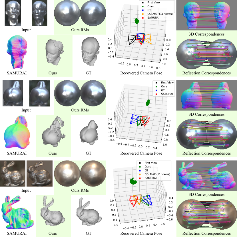
Figure 10: Reflectance maps (RMs), surface geometry, relative camera poses, and correspondences recovered from two-view real-world images.

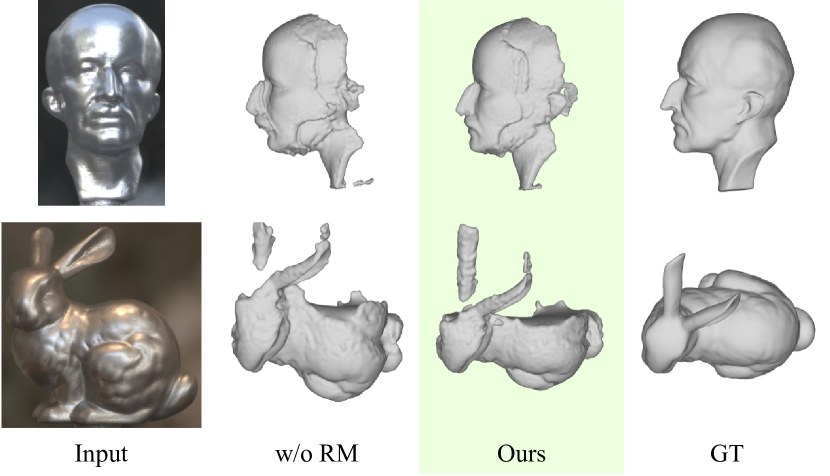
Figure 11: Effectiveness of the use of reflection correspondences.

	Planck	Horse	Bunny
COLMAP [16] (*)	15.7 deg	N/A	24.5 deg
SAMURAI [3]	5.6 deg	24.3 deg	30.5 deg
w/o RM	3.8 deg	20.2 deg	11.9 deg
Ours	1.9 deg	12.5 deg	7.2 deg

Table 2: Camera pose estimation accuracy on real-world images in the nLMVS-Real dataset [20]. (*) COLMAP [16] uses 11 view uncropped images as inputs. Please see the text for details.

D.1 Effectiveness of Reflection Correspondences

We also compared with our method “w/o RM”, a variant of our method that only leverages pixel and 3D correspondences. To obtain a unique solution without using reflection correspondences, we ignore the bas-relief ambiguity and recovered the relative rotation based on Eq. (3) in the main text. For detection of inlier 3D correspondences, we use the same RANSAC-based algorithm as one in the first-step of our camera pose estimation method.

Table 2 and Fig. 11 show quantitative and qualitative results. Note that the joint shape and camera pose recovery without reflection correspondences completely failed on the “Horse” object. In Tab. 2, we report the accuracy of our method “w/o RM” without the joint estimation for the “Horse” object. Without reflection correspondences, the recovered camera poses can be wrong and the recovered geometry can be distorted due to the bas-relief ambiguity.

References

- Belhumeur et al. [1999] Peter N. Belhumeur, David J. Kriegman, and Alan L. Yuille. The Bas-Relief Ambiguity. IJCV, 35(1):33–44, 1999.
- Bhayani et al. [2023] Snehal Bhayani, Torsten Sattler, Viktor Larsson, Janne Heikkilä, and Zuzana Kukelova. Partially Calibrated Semi-Generalized Pose from Hybrid Point Correspondences. In Proc. WACV, 2023.
- Boss et al. [2022] Mark Boss, Andreas Engelhardt, Abhishek Kar, Yuanzhen Li, Deqing Sun, Jonathan T. Barron, Hendrik P. A. Lensch, and Varun Jampani. SAMURAI: Shape And Material from Unconstrained Real-world Arbitrary Image collections. In Proc. NeurIPS, 2022.
- Chang et al. [2009] Ju Yong Chang, Ramesh Raskar, and Amit K. Agrawal. 3D Pose Estimation and Segmentation using Specular Cues. In Proc. CVPR, pages 1706–1713. IEEE Computer Society, 2009.
- Fischler and Bolles [1981] Martin A. Fischler and Robert C. Bolles. Random Sample Consensus: A Paradigm for Model Fitting with Applications to Image Analysis and Automated Cartography. Commun. ACM, 24(6):381–395, 1981.
- Harris [1991] Christopher G. Harris. Structure-from-Motion under Orthographic Projection. IJCV, 9(5):329–332, 1991.
- Horn and Sjoberg [1979] Berthold K. P. Horn and Robert W. Sjoberg. Calculating the Reflectance Map. Applied optics, 18(11):1770–1779, 1979.
- Lagger et al. [2008] Pascal Lagger, Mathieu Salzmann, Vincent Lepetit, and Pascal Fua. 3D Pose Refinement from Reflections. In Proc. CVPR. IEEE Computer Society, 2008.
- Liu et al. [2023] Yuan Liu, Peng Wang, Cheng Lin, Xiaoxiao Long, Jiepeng Wang, Lingjie Liu, Taku Komura, and Wenping Wang. NeRO: Neural Geometry and BRDF Reconstruction of Reflective Objects from Multiview Images. ACM TOG, 2023.
- Lowe [2004] David G. Lowe. Distinctive Image Features from Scale-Invariant Keypoints. IJCV, 60(2):91–110, 2004.
- Mildenhall et al. [2020] Ben Mildenhall, Pratul P. Srinivasan, Matthew Tancik, Jonathan T. Barron, Ravi Ramamoorthi, and Ren Ng. NeRF: Representing Scenes as Neural Radiance Fields for View Synthesis. In Proc. ECCV, 2020.
- Netz and Osadchy [2013] Aaron Netz and Margarita Osadchy. Recognition Using Specular Highlights. TPAMI, 35(3):639–652, 2013.
- Niemeyer et al. [2020] Michael Niemeyer, Lars Mescheder, Michael Oechsle, and Andreas Geiger. Differentiable Volumetric Rendering: Learning Implicit 3D Representations without 3D Supervision. In Proc. CVPR, 2020.
- Park et al. [2019] Kiru Park, Timothy Patten, and Markus Vincze. Pix2Pose: Pixel-Wise Coordinate Regression of Objects for 6D Pose Estimation. In Proc. ICCV, 2019.
- Schnieders and Wong [2013] Dirk Schnieders and Kwan-Yee Kenneth Wong. Camera and Light Calibration from Reflections on a Sphere. CVIU, 117(10):1536–1547, 2013.
- Schönberger and Frahm [2016] Johannes Lutz Schönberger and Jan-Michael Frahm. Structure-from-Motion Revisited. In Proc. CVPR, 2016.
- van den Oord et al. [2018] Aäron van den Oord, Yazhe Li, and Oriol Vinyals. Representation Learning with Contrastive Predictive Coding. arXiv preprint arXiv:1807.03748, 2018.
- Virtanen et al. [2020] Pauli Virtanen, Ralf Gommers, Travis E. Oliphant, Matt Haberland, Tyler Reddy, David Cournapeau, Evgeni Burovski, Pearu Peterson, Warren Weckesser, Jonathan Bright, Stéfan J. van der Walt, Matthew Brett, Joshua Wilson, K. Jarrod Millman, Nikolay Mayorov, Andrew R. J. Nelson, Eric Jones, Robert Kern, Eric Larson, C J Carey, İlhan Polat, Yu Feng, Eric W. Moore, Jake VanderPlas, Denis Laxalde, Josef Perktold, Robert Cimrman, Ian Henriksen, E. A. Quintero, Charles R. Harris, Anne M. Archibald, Antônio H. Ribeiro, Fabian Pedregosa, Paul van Mulbregt, and SciPy 1.0 Contributors. SciPy 1.0: Fundamental Algorithms for Scientific Computing in Python. Nature Methods, 17:261–272, 2020.
- Wang et al. [2021] Peng Wang, Lingjie Liu, Yuan Liu, Christian Theobalt, Taku Komura, and Wenping Wang. NeuS: Learning Neural Implicit Surfaces by Volume Rendering for Multi-view Reconstruction. In Proc. NeurIPS, pages 27171–27183, 2021.
- Yamashita et al. [2023a] Kohei Yamashita, Yuto Enyo, Shohei Nobuhara, and Ko Nishino. nLMVS-Net: Deep Non-Lambertian Multi-View Stereo. In Proc. WACV, pages 3037–3046, 2023a.
- Yamashita et al. [2023b] Kohei Yamashita, Shohei Nobuhara, and Ko Nishino. DeepShaRM: Multi-View Shape and Reflectance Map Recovery Under Unknown Lighting. arXiv preprint arXiv:2310.17632, 2023b.
- Yariv et al. [2020] Lior Yariv, Yoni Kasten, Dror Moran, Meirav Galun, Matan Atzmon, Basri Ronen, and Yaron Lipman. Multiview Neural Surface Reconstruction by Disentangling Geometry and Appearance. In Proc. NeurIPS, pages 2492–2502, 2020.
- Zhang et al. [2021a] Kai Zhang, Fujun Luan, Qianqian Wang, Kavita Bala, and Noah Snavely. PhySG: Inverse Rendering with Spherical Gaussians for Physics-based Material Editing and Relighting. In Proc. CVPR, pages 5453–5462, 2021a.
- Zhang et al. [2021b] Xiuming Zhang, Pratul P Srinivasan, Boyang Deng, Paul Debevec, William T Freeman, and Jonathan T Barron. NeRFactor: Neural Factorization of Shape and Reflectance Under an Unknown Illumination. ACM TOG, 40(6):237:1–237:18, 2021b.
- Özyeşil et al. [2017] Onur Özyeşil, Vladislav Voroninski, Ronen Basri, and Amit Singer. A Survey of Structure from Motion. Acta Numerica, 26:305–364, 2017.