Using Large Language Models for
Hyperparameter Optimization

Abstract

This paper studies using foundational large language models (LLMs) to make decisions during hyperparameter optimization (HPO). Empirical evaluations demonstrate that in settings with constrained search budgets, LLMs can perform comparably or better than traditional HPO methods like random search and Bayesian optimization on standard benchmarks. Furthermore, we propose to treat the code specifying our model as a hyperparameter, which the LLM outputs, going beyond the capabilities of existing HPO approaches. Our findings suggest that LLMs are a promising tool for improving efficiency in the traditional decision-making problem of hyperparameter optimization.

1 Introduction

Hyperparameters, distinct from the parameters directly learned throughout training, significantly influence the inductive bias of a machine learning model, thus determining its capacity to generalize effectively. The choice of hyperparameters helps dictate the complexity of the model, the strength of regularization, the optimization strategy, the loss function, and more. Due to this importance, many methods have been proposed to find strong hyperparameter configurations automatically. For example, black-box optimization methods such as random search [6] or Bayesian optimization [42, 49] have been deployed for hyperparameter optimization (HPO). Beyond black-box methods, other works further utilize the structure of the problem, e.g., are compute-environment-aware [20], compute-budget-aware [32], multi-task [52], like transfer-learning [21] or multi-fidelity [30], iterative-optimization-aware [33], online [26], or multi-objective [15]. However, these methods (a) still rely on practitioners to design a search space, which includes selecting which parameters can be optimized and specifying bounds on these parameters, and (b) typically struggle in the initial search phase ($<2^{d}$ queries for $d$-dimensional hyperparameters).

This paper investigates the capacity of large language models (LLMs) to optimize hyperparameters. Large language models are trained on internet-scale data and have demonstrated emergent capabilities in new settings [10, 44]. We prompt LLMs with an initial set of instructions – describing the specific dataset, model, and hyperparameters – to recommend hyperparameters to evaluate. Upon receiving these hyperparameters, we train the model based on the proposed configuration, record the final metric (e.g., validation loss), and ask the LLM to suggest the next set of hyperparameters. Figure 1 illustrates this iterative process.

Empirically, we employ our proposed algorithm to investigate whether LLMs can optimize 2D toy optimization objectives, where LLMs only receive loss $\mathcal{L}(\boldsymbol{x})$ at specific points $\boldsymbol{x}$. Across a range of objectives, we show that LLMs effectively minimize the loss, exploiting performant regions or exploring untested areas. Next, to analyze whether LLMs can optimize realistic HPO settings, we evaluate our approach on standard HPO benchmarks, comparing it to common methods such as random search and Bayesian optimization. With small search budgets (e.g., $10$ evaluations), LLMs can improve traditional hyperparameter tuning. We also assess the importance of using chain-of-thought reasoning [59] and demonstrate that LLMs can also perform well over longer horizons of 30 evaluations. This opens the door to many possibilities, such as using the LLM output to complement other HPO methods.

We further explore the possibilities of optimizing hyperparameters with more flexibility. Rather than adhering to a fixed set of hyperparameter configurations, we prompt LLMs to produce training code (e.g., in PyTorch) to improve validation performance. This extension alleviates the need for human specification of the hyperparameters and their search spaces. As such, code generation can help automate applying machine learning to real-world problems. The generated code provides a strong initialization and can reduce the initial search for configuration spaces that are unlikely to succeed. With a limited search budget ($5$ evaluations), our results show that code generation performs better than random search. We conclude with a discussion of language models as general-purpose hyperparameter tuning assistants, limitations, and future work.

2 Method

Figure 1: LLMs for hyperparameter optimization. In this sequential decision making setup, we prompt an LLM with the problem description and the search space. The LLM then outputs a set of hyperparameters to evaluate. The environment executes a training run with the hyperparameter setting, and then a validation metric is used to prompt the language model again.

Figure 2: Minimum validation error achieved after $10$ function evaluations from different hyperparameter optimizers on datasets from HPOBench [17]. The benchmark defines a configuration search space on neural networks for learning rates, $\ell_{2}$ regularization, width, depth, and batch size. A large language model (GPT-4 Turbo) performs well compared to random search and Bayesian optimization ($BO$) with Gaussian process ($GP$) and random forest ($RF$) surrogate models. We also conduct experiments to tune the hyperparameters for logistic regression, support vector machines (SVMs), and random forests, with aggregate results in Table 1.

2.1 Background

Hyperparameter optimization can be formulated as a bilevel optimization problem:

$$\boldsymbol{\lambda}^{\star} =\operatorname*{arg\,min}_{\boldsymbol{\lambda}}\mathcal{L}_{V}^{*}\left(\boldsymbol{\lambda}\right)=\operatorname*{arg\,min}_{\boldsymbol{\lambda}}\mathcal{L}_{V}\left(\boldsymbol{\lambda},\mathbf{w}^{\star}\left(\boldsymbol{\lambda}\right)\right)$$ (1)

$$\text{ s.t. }\mathbf{w}^{\star}\left(\boldsymbol{\lambda}\right) =\operatorname*{arg\,min}_{\mathbf{w}}\mathcal{L}_{T}\left(\boldsymbol{\lambda},\mathbf{w}\right),$$ (2)

where $\mathcal{L}_{T}$ and $\mathcal{L}_{V}$ are training and validation objectives, and $\boldsymbol{\lambda}$ and $\mathbf{w}$ are hyperparameters and the model parameters, respectively. Intuitively, the objective – i.e., the validation loss with best-responding parameters $\mathcal{L}_{V}^{*}$ – aims to find the hyperparameters that minimize the validation loss when the training objective is trained to convergence. Hyperparameter optimization can be done in sequential fashion, where a proposal $\boldsymbol{\lambda}_{n}$ depends on the sequence of prior values $\{\boldsymbol{\lambda}_{1},\boldsymbol{\lambda}_{2},\dots,\boldsymbol{\lambda}_{n-1}\}$ and their validation losses.

For instance, Bayesian Optimization [42, 49] builds a probabilistic model, such as a Gaussian Process, to map hyperparameters $\boldsymbol{\lambda}$ to the validation loss $\mathcal{L}_{V}(\boldsymbol{\lambda},\mathbf{w}^{*}(\boldsymbol{\lambda}))$. This approach iteratively selects the next hyperparameters to evaluate by optimizing an acquisition function that balances exploration and exploitation, thereby converging to the optimal hyperparameters $\boldsymbol{\lambda}^{*}$ that minimize the validation loss. In a limited budget setting, practitioners often employ a trial-and-error “manual" search, choosing hyperparameters based on prior knowledge or experience [61]. In this paper, we assess the ability of large language models in this role, hypothesizing they will be effective as they have been trained on internet-scale data and have demonstrated emergent capabilities in new settings [10, 44].

2.2 LLMs for Hyperparameter Optimization

We now describe our approach in more detail. We first address the case when the hyperparameters search space is known. We prompt an LLM by describing the problem and the search space. The LLM outputs a hyperparameter setting to evaluate. We then repeatedly alternate between two steps: (1) evaluating the current hyperparameter setting, and (2) prompting the LLM with the validation metric (e.g., loss or accuracy) to receive the next set of hyperparameters. This continues until our search budget is exhausted. We illustrate this process in Figure 1 and list the prompts that we use in Appendices B and D. Note that our prompts provide a high-level overview of the machine learning problem setup, the hyperparameters that can be tuned, and, if given, their associated search spaces.

⬇

### 1. Chat prompting

[User: <<Machine learning problem description>>. Provide a config in JSON format. Config:

(Assistant: <<generated hyperparameter configuration>>

User: The validation loss was <<L>>. Provide the next config in the same format.

) x N]

### 2. Single message prompting

[User: <<Machine learning problem description>>. Here is what we have tried so far:

<<Config 1>> <<Loss 1>>

<<Config 2>> <<Loss 2>>

...

<<Config N>> <<Loss N>>

Provide the next config in JSON format. Config:]

Figure 3: Two ways to prompt the language model. Angular brackets vary with the problem or are dependent on what was generated in previous steps. Note that both approaches end with a user message so that the language model generates the next response.

More concretely, we consider two ways to prompt the model, following the popular “chat” interface [56, 44] where users prompt the model with a dialogue consisting of “user” and “assistant” messages, depicted in Figure 1. The models we use generate tokens sampled according to an input temperature, terminating at a stop token. We prompt the model with the entire conversational history of messages, so the number of messages sent in the $n$-th prompt scales linearly with the number of steps. This is because every new step contains two additional messages: the previous LLM response and the validation metrics from executing a training run from the hyperparameters in the response. The number of tokens increases by the number of tokens representing the validation metrics and configuration. We denote this approach the “chat” prompt.

An alternative is to compress the previous search history into a single initial message. The single message contains the problem description and lists the configurations’ history and corresponding validation metrics. This approach represents a more compact state representation, especially if we use chain-of-thought reasoning [59] prompting strategies explored in our experiments. The inference cost on compressed messages is cheaper than in the prior approach. Empirically, we observe that the two approaches achieve similar performance. We denote this approach the “compressed” prompt.

When the search space is unknown, we can prompt an LLM to generate code for the model and optimizer, effectively providing a hyperparameter setting to evaluate. In this case, the environment executes the generated code and provides the resulting output to the LLM. We use the prompt in Appendix C. If the code fails to produce a validation accuracy, then we can re-prompt with the error message. Note that code generation can also be viewed as hyperparameter tuning, where the hyperparameter is the input string representing the code.

3 Related Work

Hyperparameter Optimization (HPO).

Finding the optimal hyperparameter settings is crucial to achieving strong performance in machine learning [6, 50]. We refer readers to Feurer and Hutter [18] and Bischl et al. [8] for a general introduction to HPO. Initial research mainly explored model-free techniques such as grid and random search [6]. More advanced methods leverage multi-fidelity optimization – often by using that our optimization is an iterative process. For example, Hyperband [33] and the Successive Halving [27] introduced multi-armed bandit approaches to allow for the early stopping of less promising hyperparameter configurations. These methods are easy to parallelize and have shown promising results in practice, but are dependent on random processes and do not fully leverage the HPO structure.

Bayesian Optimization (BO) [42, 25, 50, 7, 49] builds a surrogate model from past function evaluations to choose promising future candidates. BO further models uncertainty, leveraged by optimizing an acquisition function instead of the loss directly. Since the initial successes of BO in optimizing hyperparameters, numerous tools have been developed to optimize the pipeline for improved efficiency and adaptability [4, 29, 5, 35]. However, BO requires building an inductive bias in conditional probability, is heavily influenced by the choice of surrogate model parameters [34], and, importantly, faces scalability problems with an increase in the number of hyperparameters being tuned or the number of past function evaluations. Gradient or conditioning-based methods [41, 19, 37, 40, 2, 38, 47, 3] present a more scalable and efficient solution for HPO. Nevertheless, they are often challenging to implement, require the objective to be differentiable, and must be deployed in the same location as the underlying model, which makes them less appealing as general HPO solvers. A related approach is OptFormer [13], which finetunes Transformers on a large offline dataset to transfer learn a surrogate used for gradient-based HPO.

Decision making with LLMs.

Large language models (LLMs) have proven to be exceptionally valuable in a variety of practical domains [22, 36], showing surprising emergent abilities, including in-context learning and chain-of-thought reasoning [10, 59, 44]. Although LLMs are known to occasionally give confident but incorrect answers [28], they are also shown to have reasoning capabilities, especially when explicitly guided to [43, 59, 31]. Recent studies have used LLMs for optimization [60], such as finding the best prompt for the downstream task or integrating LLMs into the general AutoML pipeline [11, 24, 39, 62, 63]. For example, Zheng et al. [63] uses similar prompting strategies for neural architecture search (NAS) and demonstrates that LLMs can find competitive architectures on NAS benchmarks [51].

4 Results

We report our results for tuning hyperparameters on eight different datasets and four models (neural nets, SVMs, random forests, and logistic regression) from the HPOBench benchmark for hyperparameter optimization [17]. We then analyze low-dimensional optimization problems to understand and visualize the LLM trajectories in a simpler setting and then discuss how our approach can be applied to code generation.

4.1 Hyperparameter Optimization on HPOBench

We report results on the HPOBench [17] benchmark, which defines search spaces for various models on publicly available OpenML AutoML benchmarks. Eggensperger et al. [17] show that the benchmarks yield different hyperparameter-loss landscapes and are effective for benchmarking algorithm performance. We used the first $8$ datasets provided and tuned hyperparameters for the algorithms implemented in Sklearn: logistic regression, support vector machines (SVMs), random forests, and neural networks [45], resulting in $32$ different tasks. We tune $2$ hyperparameters for SVMs, $2$ for logistic regression, $4$ for random forests, and $5$ for neural networks [17]. Search space details can be found in Appendix B, as well as figures of results on each task. We compare the following HPO approaches:

LLMs. We use the most recent time-stamped versions of GPT-3.5 and GPT-4 models from OpenAI in our initial experiments: gpt-3.5-turbo-0613 and gpt-4-0613 with temperature 0. Since GPT-4 Turbo was released after our initial experiments, we also conducted experiments with the model gpt-4-1106-preview and found it performed better at less than half the price of GPT-4.

Random. Random search often outperforms grid and manual search, thriving when the hyperparameter space has low effective dimensionality [6]. The design spaces of a given benchmark dictate where we should sample – e.g., log-uniformly for regularization hyperparameters in $\mathbb{R}^{+}$ or from a discrete set such as the number of neural network layers. We randomly sample $500$ configurations for each model and dataset combination, evaluate the corresponding losses, and then use a bootstrapped sample to estimate the loss on a given budget.

Bayesian Optimization (BO). We evaluate two Bayesian HPO methods in the SMAC3 library [35] that use random forest and Gaussian processes as surrogate models.

In Table 1, we report aggregated results comparing two LLMs, random search, and two BO algorithms with different surrogate models. We compare the difference in validation error versus random search ($0.2$ to $0.1$ is a $50\%$ improvement). Every algorithm has a search budget of $10$ function evaluations. As a summary metric, we report the mean and median improvement in the $32$ tasks of each algorithm versus random search. Full results detailing the performance of each dataset and model are in Figure 2 and Figure 6. GPT-4 Turbo beats random search most frequently and achieves the highest mean and median improvement. When we compare the mean rank for the five search algorithms across the $32$ tasks – again, GPT-4 Turbo is consistently better.

Table 1: We summarize the performance of various HPO Algorithms versus random search on $8$ datasets and $4$ search spaces tuning hyperparameters for logistic regression, SVMs, random forests, and neural networks. Bayesian optimization uses Gaussian process ($GP$) and random forest ($RF$) surrogate models. For all tasks, we use $10$ function evaluations. As summary metrics, we report how often each method beats random search (GPT-4 Turbo beats random search 81.25% of the time). We also compute the change in validation error for each optimizer versus random search and report the median and mean change across $32$ tasks. The mean rank is computed between the $5$ HPO approaches and random search, i.e. each method is assigned a rank between $1$ and $6$ on a task. The mean rank for random across the 32 tasks is $4.00$. Figure 6 shows the detailed performance on the other tasks.

Model	Beats Random ($\uparrow$)	Median Change ($\uparrow$)	Mean Change ($\uparrow$)	Mean Rank ($\downarrow$)
GPT-4 Turbo	81.25%	13.70%	19.83%	2.42
GPT-4	68.75%	4.58%	8.54%	3.48
GPT-3.5 Turbo	43.75%	-0.82%	-13.58%	3.84
$\text{Bayes Opt}_{RF}$	56.25%	2.11%	5.86%	3.45
$\text{Bayes Opt}_{GP}$	50.00%	-0.01%	-8.28%	3.80

Table 2: Chain-of-thought reasoning prompting may offer modest improvement versus prompting a model to output the next set of hyperparameters immediately.

Model	Beats Random ($\uparrow$)	Median Change ($\uparrow$)	Mean Change ($\uparrow$)
GPT-4 Turbo CoT	81.25%	13.70%	19.83%
GPT-4 Turbo	81.25%	15.58%	21.23%
GPT-4 CoT	68.75%	4.58%	8.54%
GPT-4	65.62%	3.43%	11.55%
GPT-3.5 Turbo CoT	43.75%	-0.82%	-13.58%
GPT-3.5 Turbo	40.62%	-3.19%	-117.12%

Table 3: Evaluating performance on a longer trajectory of $30$ function calls. GPT-4-Turbo still maintains good performance, suggesting that it is capable of selecting problem-specific hyperparameter settings. The mean rank between all $5$ methods (each row + random) is $3$.

Model	Beats Random ($\uparrow$)	Median Change ($\uparrow$)	Mean Change ($\uparrow$)	Rank ($\downarrow$)
GPT-4 Turbo CoT	78.12%	12.10%	18.27 %	2.72
GPT-4 Turbo	90.62%	18.94%	22.34 %	2.22
$\text{Bayes Opt}_{RF}$	71.88%	5.91%	14.63 %	3.06
$\text{Bayes Opt}_{GP}$	84.38%	11.80%	21.07 %	2.75

How important is chain-of-thought reasoning?

In Table 2, we evaluate the effects of chain-of-thought [59] on performance. To elicit reasoning, our intermediate messages to the language model are:

⬇

loss = {loss:.4e} Write two lines as follows:

Analysis: Up to a few sentences describing what worked so far and what to choose next

Config: (JSON config)

The loss is expressed in scientific notation to four decimal places. See Appendix B for complete details on the prompts. We see that including reasoning has a large positive impact on GPT-3.5 and a marginal impact on GPT-4. Reasoning chains can be informative for a practitioner at the cost of additional tokens. Below is a snippet of GPT-4 reasoning when tuning hyperparameters for a neural network.

• (loss $0.193$) GPT-4: The loss remained the same despite changes in the hyperparameters. This suggests that the model might not be sensitive to these parameters or has reached a local minimum. We should try a more drastic change in the learning rate and depth. <proposed config consistent with reasoning>

• (loss $0.215$) GPT-4: The loss increased, indicating that the last configuration was not beneficial. The increase in learning rate and the decrease in depth might have caused the model to overshoot the minimum. Let’s try reducing the learning rate and increasing the depth.

We provide additional full trajectories in the Appendix F. We qualitatively observe reasoning that trades off between exploration and selecting a strong final value.

Longer trajectories

We additionally evaluate our approach on a longer time horizon, with $30$ function queries, and show the results in Table 3. Here, we use the “compressed” prompt described in Section 2: we prompt the LLM with a single message at each step, showing the entire history of hyperparameter configurations and losses. A longer search trajectory has a reduced dependency on initialization and requires a better search algorithm for good performance. GPT-4 Turbo still compares favorably with other approaches. Qualitatively, the reasoning generated by the language model is a useful summary of experimental results and the relative importance of different hyperparameters. For example, when tuning a random forest, we get the following reasoning:

• GPT-4-Turbo: The lowest loss so far is with Config 9, which suggests that a combination of a slightly deeper tree (max_depth: 15), a moderate number of features (max_features: 0.5), and a higher number of samples at the leaf nodes (min_samples_leaf: 4) and for splitting (min_samples_split: 8) is beneficial. The loss has not improved significantly with changes to the max_depth beyond the default, so we should explore other parameters more. We can try increasing the min_samples_leaf further since increasing it from 1 to 4 improved the performance, and we can also experiment with a different max_features value to see if it affects the loss.

Additionally, we run a preliminary experiment to assess if LLMs can be useful to initialize Bayesian optimization – we find that for a search trajectory of length 30, using the LLM proposed configurations for the first ten steps improves or matches performance on 21 of the 32 tasks ($65.6\%$) for Bayesian optimization with a random forest surrogate function.

4.2 Code generation

Code generation offers a flexible paradigm to specify the configuration space for hyperparameter tuning. In this setup, we treat the model and optimizer source code as hyperparameters tuned by the LLM. We use code generation as a method to circumvent requiring a specific configuration space to search over. The code generation approach is evaluated against random search and LLMs with a fixed, configuration-based search space. The baseline methods are provided with a space, which includes the depth and width of the network, the batch size, learning rate, and weight decay. To minimize the risk of data leakage issues where the LLM was trained on good hyperparameter settings for our dataset, we used a recent Kaggle NYC Taxi dataset [54, 55] for our experiments. We provide our prompts and additional details in Appendix C.

On the first tuning iteration, we ask the LLM (gpt-4-1106-preview) to output source code for the model and optimizer, which implicitly also requires specifying the hyperparameters. This code is generated as functions that take in hyperparameters as arguments. In later iterations, the hyperparameter tuning is done by asking the LLM to generate functions calls with specific arguments. The model is run with the given settings, and the LLM receives the validation loss and the average training losses during each epoch as feedback.

Table 4 reports the minimum test loss achieved using a fixed search budget of $5$ evaluations, which simulates the results of the initial search phase during hyperparameter tuning. We randomly sample 200 configurations and use a bootstrapped sample to estimate the standard error for a random search. Figure 4 reports the minimum test loss found at each step and illustrates that code generation obtains better initial settings than competing approaches.

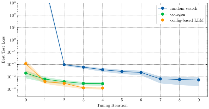
Figure 4: Test loss trajectory comparison with a standard error displayed over $5$ runs. We randomly sample 200 configurations and use a bootstrapped sample to estimate the standard error for a random search. Code generation and configuration-based search both compare favorably to random search.

Table 4: Minimum test loss after $5$ tuning iterations. We report the mean and standard error for code generation and the config-based LLM across 5 runs.

Method	Min Test Loss ($\downarrow$)
Random search	$3.757\times 10^{-3}\pm 1.172\times 10^{-3}$
Code generation	$2.754\times 10^{-4}\pm 9.241\times 10^{-5}$
Config-based LLM	$1.218\times 10^{-4}\pm 2.959\times 10^{-5}$

4.3 2-Dimensional Landscapes

To evaluate whether LLMs can reason about optimization choices, we study a set of 2-dimensional toy test functions commonly used in optimization: Rosenbrock [48], Branin [16], Himmelblau [23], and Ackley [1]. For each test function $f$, we consider optimizing $f(\boldsymbol{x})$ and also $f(\boldsymbol{x}-\boldsymbol{c})$, where $\boldsymbol{c}$ is a fixed constant, with $\boldsymbol{c}_{i}\sim\mathcal{U}(0,1)$, to mitigate the LLM’s potential to memorize the original $f$. Also, we benchmark performance on a well-conditioned and ill-conditioned quadratic. We provide the experimental details and the explored prompts in Appendix D.

We search for optimal solutions using LLMs as an optimizer with GPT-4. While these problems can be considered black-box optimization, we can also pose them as HPO to the LLM, using the same prompts in Figure 1 for consistency. We show the performance of a single fixed seed and temperature $0$ in Figure 5. Performance across $3$ seeds outperforms random search in most tasks, as shown in Table 7. Moreover, inspecting the trajectories and reasoning chains shown in Appendix F, we qualitatively observe different behaviors that may characterize a strong search algorithm: initial exploration around the center and boundaries of the search space; a line-search type algorithm to probe function behavior; and reasoning that trades off between exploration and selecting a performant final value. However, performance can be inconsistent between random seeds, as shown in Table 6.

We use prompts with minimal details to gain intuition on this HPO approach and to evaluate our LLM approach on problems with less complexity. Inspecting the trajectories, we see room for more specific prompts. For example, the LLMs re-explored previously evaluated points. We obtain the same or better performance in $8$ of the $10$ tasks by adding a sentence stating that the functions are deterministic, shown in Table 8. We speculate that HPO performance can generally be improved with more details on the problem setting in the prompt.

Figure 5: The LLM optimizer effectively optimizes the function in most situations with few function evaluations, even when we apply random argument shifts to mitigate memorization.

5 Discussion

When performing HPO, LLMs can extend beyond fixed configuration spaces for hyperparameter tuning, as they can offer interactive help to debug and improve models using natural language. We highlight some limitations and potential applications.

5.1 Limitations

Limited Context Length.

A primary limitation of our prompting-based approach is the limited context length. LLMs typically have a predetermined context window size and cannot process prompts exceeding this limit in the token count. As we incorporate the history of previously tried suggestions from the LLMs, the number of input tokens in the prompt increases with each additional round of hyperparameter optimization and the total number of hyperparameters being tuned. Allocating more budgets to the hyperparameters requires longer context lengths. Advancements in research aimed at extending the context length for LLMs [12] can potentially improve results by allowing a higher budget for hyperparameter optimization. Indeed, we see that GPT-4-Turbo already has a context length of 128k, significantly longer than previous OpenAI models.

Challenges with Reproducibility.

The exact inference procedures for LLMs like GPT-4 [44] are not publicly disclosed, making replicating the results in this work potentially challenging. For example, although GPT-4 should ideally give the same results when the sampling temperature is set to $0$, this is not always true. For future studies, using open source LLMs [53, 14, 56, 57] to establish a benchmark with reproducible results would be beneficial. We focus on the current most general-purpose capable models, as most open-source models perform worse than GPT-3.5 on benchmarks.

Possibility of Dataset Contamination.

It is possible that some of the evaluation benchmarks used were part of the LLM training data. However, previous research suggests that such contamination might not critically influence overall performance [46]. Building more private data sets unseen by LLM during training would be valuable for future studies or even synthetic datasets like our quadratic experiments. Additionally, we emphasize that our prompting process only provides the output of a function and does not contain any information about the benchmark, reducing the likelihood of exact memorization.

Cost.

It can be costly to conduct a full-scale HPO experiment with GPT-4. For example, executing $32$ tasks using chain-of-thought reasoning on HPOBench costs approximately $\$8$ USD as of September 2023. This cost can increase further when using more budget, but can be reduced by using the “compressed" prompt. We believe this burden will be alleviated as the models improve to be both capable and cost-efficient.

5.2 LLMs as a Hyperparameter Tuning Assistant

We run initial experiments to demonstrate the potential of an LLM as a general-purpose assistant for training pipelines. In Figure 7, LLMs provide useful feedback for the error messages, which is infeasible with traditional approaches. However, this can suffer from the challenges that affect current language models, such as hallucinations [9]. In Figure 8, the LLM assumes that the user has a neural network and suggests regularization, which may be unhelpful if the model is underfitting. Exploring this paradigm further is an exciting direction for future work.

Appendix A Appendix

Our appendix includes details on 2-dimensional landscape experiments in Section D, HPOBench experiments in Section B, dialogues of using LLMs as Tuning Assistants in Section E, and trajectories of LLM responses in Section F.

Appendix B HPOBench

B.1 Prompts

Our initial prompt is the concatenation of a generic message and the Sklearn documentation for specific hyperparameters. This is the initial message we use for all models.

beginning

You are helping tune hyperparameters for a {model}. Training is done with Sklearn. This is our hyperparameter search space:

These search space descriptions are copied verbatim from Sklearn and the benchmark configuration.

middle

svm

C, regularization parameter. The strength of the regularization is inversely proportional to C. Must be strictly positive. The penalty is a squared l2 penalty. Type: UniformFloat, Range: [0.0009765625, 1024.0], Default: 1.0, on log-scale
gamma, Kernel coefficient for rbf, Type: UniformFloat, Range: [0.0009765625, 1024.0], Default: 0.1, on log-scale

logistic regression

alpha, constant that multiplies the regularization term. The higher the value, the stronger the regularization. Type: UniformFloat, Range: [1e-05, 1.0], Default: 0.001, on log-scale
eta0, The initial learning rate for the adaptive schedule. Type: UniformFloat, Range: [1e-05, 1.0], Default: 0.01, on log-scale

random forest

max_depth, the maximum depth of the tree. Type: UniformInteger, Range: [1, 50], Default: 10, on log-scale
max_features, the number of features to consider when looking for the best split. Type: UniformFloat, Range: [0.0, 1.0], Default: 0.5
min_samples_leaf, the minimum number of samples required to be at a leaf node. Type: UniformInteger, Range: [1, 20], Default: 1
min_samples_split, the minimum number of samples required to split an internal node. Type: UniformInteger, Range: [2, 128], Default: 32, on log-scale

neural net

alpha, l2 regularization, Type: UniformFloat, Range: [1e-08, 1.0], Default: 0.001, on log-scale
batch_size, Type: UniformInteger, Range: [4, 256], Default: 32, on log-scale
depth, Type: UniformInteger, Range: [1, 3], Default: 3
learning_rate_init, Type: UniformFloat, Range: [1e-05, 1.0], Default: 0.001, on log-scale
width, Type: UniformInteger, Range: [16, 1024], Default: 64, on log-scale

end

We have a budget to try 10 configurations in total. You will get the validation error rate (1 - accuracy) before you need to specify the next configuration. The goal is to find the configuration that minimizes the error rate with the given budget, so you should explore different parts of the search space if the loss is not changing. Provide a config in JSON format. Do not put new lines or any extra characters in the response. Example config: {"C": x, "gamma": y} Config:

B.2 Transition Messages

After receiving the initial config, we evaluate the hyperparameters and prompt the language model with the following:

⬇

loss = {loss:.4e}. Specify the next config, do not add anything else in your response. Config:

Here “{loss:.4e}" represents the loss in scientific notation with 4 decimal places.

After that, we use one of the following prompts, where the validation loss is updated based on the result of the training run.

⬇

### Chain of Thought (CoT)

loss = {loss:.4e} Write two lines as follows:

Analysis: Up to a few sentences describing what worked so far and

what to choose next

Config: (JSON config)

### Normal (No CoT)

loss = {loss:.4e}. Specify the next config.

Finally, on the last attempt before our budget is exhausted, we preface the message with “This is the last try." These prompts seemed natural to try, and we did not adjust them beyond adding “do not add anything else" to ensure that the language model output is easily parsable.

B.3 Results

In Figure 6, we show the validation accuracy achieved on each task.

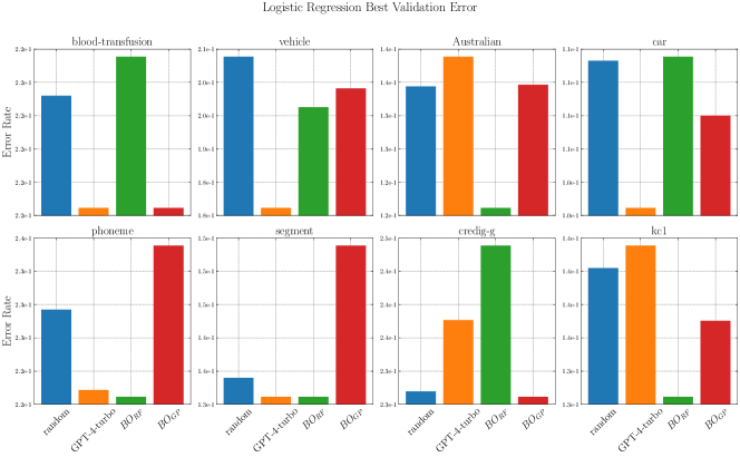
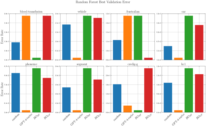
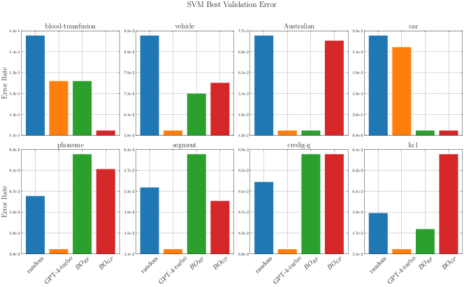
Figure 6: Results on logistic regression, random forests, and SVMs.

B.4 Additional Results

We consider the effect of appending a system prompt “You are a machine learning expert" in Table 5. We use this prompt throughout the rest of the experiments, following the idea of conditioning on good performance [64].

Table 5: Evaluating effects of system prompt.

Model	Beats Random ($\uparrow$)	Median Change ($\uparrow$)	Mean Change ($\uparrow$)
Expert prompt	90.62%	7.75%	23.23 %
Non-expert prompt	81.25%	13.79%	22.36 %

Appendix C Code Generation

This is the initial prompt we use for code generation:

⬇

I’m going to use your abilities to generate a model and tune its hyperparameters such that it performs well on a Kaggle challenge.

{dataset.problem_description}

You have {dataset.in_features} input features.

The names of the features in the dataset are: {dataset.X_columns}

The target variable is: {dataset.y_columns[0]}

You may assume that the dataset already preprocessed and available as a DataLoader object.

I want you to write PyTorch code that creates a model and optimizer.

Write everything in one function that is called ‘make_model_and_optimizer‘.

Later I will ask you to call this function so make sure it does not reference any global variables.

Also make sure that you include all the hyperparameters that you anticipate needing to tune later as arguments into this function.

Favour using primitive or built-in types and avoid using Callable or Module types as arguments to this function.

Be sure to include a short docstring and type annotations.

Finally, write a short sentence explaining your reasoning.

Format your output as follows:

reasoning: <your reasoning here>

code:

‘‘‘python

<your code here>

‘‘‘

The make_model_and_optimizer function is then parsed and validated. This is done by first checking that it is valid Python code, and then by checking its function signature to make sure that the function arguments and the outputs are as specified. If these constraints are not met, the error is fed back into the LLM, and it regenerates the code.

The agent now tunes hyperparameters it has specified for this function by making calls to it. This is done by taking advantage of the function calling feature in the OpenAI API to get our LLM to directly output a call into this function.

Here is the tuning prompt:

⬇

Now let’s tune the hyperparameters of your model.

Give me instances of a both the model and an optimizer by making

a call to ‘make_model_and_optimizer‘.

Use hyperparameters that you think will perform well on the validation set.

I will then train the model and give you feedback on how well it performs.

You have {search_budget} iterations to tune your model.

Your respone should just be one function call to

‘make_model_and_optimizer‘.

After training the model with the proposed settings, we provide feedback to the model using the following prompt:

⬇

Here is the output of your code:

training loss over each epoch:

{’, ’.join([f’{l:.3f}’ for l in feedback.train_losses])}

validation loss: {feedback.val_loss:.3f}

Based on this, make a new call to ‘make_model_and_optimizer‘

with hyperparameters that you think will perform better

on the validation set.

The baseline methods are given the following configuration space to optimize:

⬇

alpha, l2 regularization, Type: UniformFloat, Range: [1e-08, 1.0], Default: 0.001, on log-scale

batch_size, Type: UniformInteger, Range: [4, 256], Default: 32, on log-scale

depth, Type: UniformInteger, Range: [1, 3], Default: 3

learning_rate_init, Type: UniformFloat, Range: [1e-05, 1.0], Default: 0.001, on log-scale

width, Type: UniformInteger, Range: [16, 1024], Default: 64, on log-scale

Appendix D 2-dimensional Landscape Experiment details

D.1 Prompts

Prompt 0 is a practical description of the problem as black-box optimization.

⬇

You are optimizing a function with two inputs. x1 must be in range {search_space[’x1’]\. x2 must be in range {search_space[’x2’]}. I want you to predict values that minimize the loss of the function; I will tell you the value of the function before you try again. Do not put new lines or extra characters in your response. Format your output with json as follows: {{"x": [x1, x2]}}

Prompt 1 adds one sentence to include the compute budget.

⬇

You are optimizing a function with two inputs. x1 must be in range {search_space[’x1’]}. x2 must be in range {search_space[’x2’]}. I want you to predict values that minimize the loss of the function; I will tell you the value of the function before you try again. Do not put new lines or extra characters in your response. We have a total of {budget} evaluations. Format your output with json as follows: {{"x": [x1, x2]}}\n

Prompt 2 is similar to the second, but frames the problem as hyperparameter optimization.

⬇

You are helping tune hyperparameters to minimize loss. x1 must be in range {search_space[’x1’]}. x2 must be in range {search_space[’x2’]}. I want you to predict values that minimize the loss of the function; I will tell you the value of the function before you try again. Do not put new lines or extra characters in your response. We have a total of {budget} evaluations. Format your output with json as follows: {{"x": [x1, x2]}}\n

We also study Prompt 3 which adds a sentence: “The training process is deterministic and yields a nonnegative loss."

Toy Function	Prompt 0	Prompt 1	Prompt 2	Prompt 2 ($T=0$)
ack	0.0, 0.0, 0.0	0.0, 0.0, 0.0	0.0, 0.0, 0.0	0.0, 0.0, 0.0
shifted_ack	1.81, 2.52, 2.83	2.19, 2.19, 2.19	4.37, 2.83, 1.77	1.77, 1.86, 4.48
bran	10.82, 2.88, 3.09	1.03, 9.87, 1.94	9.87, 9.87, 0.5	1.94, 3.91, 0.5
shifted_bran	15.54, 15.8, 18.68	7.79, 1.04, 3.26	2.39, 9.9, 50.04	3.26, 5.58, 9.9
rosen	1.0, 1.0, 1.0	1.0, 0.0, 1.0	1.0, 0.0, 1.0	0.0, 1.0, 0.0
shifted_rosen	7.03, 7.03, 5.3	0.78, 167.43, 215.4	2.99, 215.4, 0.78	0.53, 163.86, 15.37
himmel	0.0, 8.12, 8.12	2.0, 8.12, 106.0	8.12, 8.12, 26.0	8.12, 8.12, 8.12
shifted_himmel	4.57, 4.57, 4.57	47.07, 14.46, 47.07	47.07, 152.1, 1.58	16.99, 47.07, 47.07
quad2d	0.44, 28.15, 0.44	11.24, 28.15, 12.75	0.72, 0.32, 0.32	1.45, 0.37, 28.15
quad2d_illcond	52.35, 51.45, 51.14	51.45, 51.45, 51.45	18.45, 0.65, 51.21	51.45, 51.14, 0.65

Table 6: Minimum loss achieved in 10 iterations on 3 different seeds at temperature 0.1. We also run the experiments for Prompt 2 with temperature 0. Note that there is randomness in the results even at temperature 0.

Toy Function	Prompt 0	Prompt 1	Prompt 2	Prompt 2 ($T=0$)	Random
ack	0.0	0.0	0.0	0.0	5.28 $\pm$ 1.73
shifted_ack	2.39	2.19	2.99	2.7	5.26 $\pm$ 1.74
bran	5.6	4.28	6.75	2.12	5.83 $\pm$ 5.57
shifted_bran	16.68	4.03	20.78	6.25	7.13 $\pm$ 6.00
rosen	1.0	0.67	0.67	0.33	481.34 $\pm$ 998.30
shifted_rosen	6.46	127.87	73.06	59.92	618.82 $\pm$ 1691.99
himmel	5.42	38.71	14.08	8.12	20.39 $\pm$ 19.93
shifted_himmel	4.57	36.2	66.92	37.04	21.47 $\pm$ 20.00
quad2d	9.68	17.38	0.46	9.99	4.72 $\pm$ 5.76
quad2d_illcond	51.65	51.45	23.44	34.41	15.14 $\pm$ 17.61

Table 7: Average minimum loss achieved in 10 iterations on 3 different seeds at temperature 0.1. We also run the experiments for Prompt 2 with temperature 0. Note that there is randomness in the results even at temperature 0. We report the mean and standard deviation for random across 1000 trials

Toy Function	Prompt 2	Prompt 3
ack	0.0	0.0
shifted_ack	2.7	2.19
bran	2.12	3.57
shifted_bran	6.25	1.23
rosen	0.33	0.33
shifted_rosen	59.92	129.31
himmel	8.12	6.05
shifted_himmel	37.04	36.21
quad2d	9.99	0.87
quad2d_illcond	34.41	27.08

Table 8: Average minimum loss achieved in 10 iterations on 3 different seeds at temperature 0. Note that there is randomness in the results even at temperature 0. Prompt 3 adds a sentence “The training process is deterministic and yields a nonnegative loss." to Prompt 2. This achieves the same or better performance on $8$ of the $10$ tasks.

Appendix E LLMs as Tuning Assistants

Large language models offer exciting potential for hyperparameter tuning as they can offer interactive help to debug and improve models, using natural language. We highlight some potential applications and limitations. We show the temperature 0 responses from different language models.

In Figure 7, LLMs provide useful feedback to someone encountering an error message, which is infeasible with traditional approaches. A user can also seek additional clarification after implementing suggestions. In Figure 8, we show a potential shortcoming of this approach. The LLMs generated content assumes the user is using a neural network and also suggests using regularization (which may be unhelpful if the model is underfitting); an expert would potentially respond by first requesting clarification from the user (e.g. what model they are training, and specifics on validation and training performance).

Question: I’m using Adam with a learning rate of 0.1 to train a neural network and get a NaN error. What should I do?

GPT-3.5-Turbo:

If you are encountering a NaN (Not a Number) error while training a neural network with Adam optimizer and a learning rate of 0.1, it typically indicates that the gradients have exploded or become too large. Here are a few steps you can take to address this issue:

1. Reduce the learning rate: A high learning rate can cause the gradients to become unstable and result in NaN errors. Try reducing the learning rate to a smaller value, such as 0.01 or 0.001, and see if the issue persists.

2. Check for numerical instability: NaN errors can also occur due to numerical instability in the network. Ensure that your input data is properly normalized and that there are no extreme values or outliers that could cause instability.

3. Implement gradient clipping: Gradient clipping is a technique that limits the magnitude of the gradients during training. By setting a maximum threshold for the gradient values, you can prevent them from becoming too large. This can help mitigate the NaN error. Most deep learning frameworks provide built-in functions for gradient clipping.

4. Check for bugs in your code: Review your code implementation to ensure there are no bugs or mistakes that could lead to NaN errors. Double-check the loss function, network architecture, and any custom layers or operations you have implemented.

5. Use regularization techniques: Regularization methods like L1 or L2 regularization, dropout, or batch normalization can help stabilize the training process and prevent NaN errors. Consider applying appropriate regularization techniques to your network.

6. Verify your data: NaN errors can also occur due to problematic data. Check your dataset for missing values, corrupted samples, or any other data-related issues that could lead to NaN errors.

7. Monitor the network’s behavior: During training, keep an eye on the loss values and gradients. If you notice sudden spikes or extremely large values, it can indicate a problem. You can also try visualizing the gradients to identify any abnormalities.

By following these steps, you should be able to diagnose and address the NaN error in your neural network training.

GPT-4:

Getting a NaN error during training usually indicates that your model is diverging, and the weights are becoming too large to represent. This is often due to a too high learning rate. Here are some steps you can take to resolve this issue:

1. Reduce the learning rate: A learning rate of 0.1 is quite high for the Adam optimizer. Try reducing it to 0.001 or 0.0001.

2. Gradient Clipping: If your model is still diverging after reducing the learning rate, you might want to try gradient clipping. This is a technique to prevent exploding gradients by capping them at a certain value.

3. Check your data: Make sure there are no NaN or infinite values in your input data. Also, check if your data is properly normalized. Large input values can also cause the model to diverge.

4. Check your model architecture: Make sure your model architecture is appropriate for your task. If your model is too complex, it might overfit and diverge.

5. Regularization: If your model is overfitting, you might want to add some form of regularization, like dropout or weight decay.

6. Check your loss function: Make sure your loss function is appropriate for your task and correctly implemented. Some loss functions can produce NaN values if not used correctly.

Remember, debugging a neural network often involves a lot of trial and error. Don’t be discouraged if the first thing you try doesn’t work. Keep experimenting and you’ll eventually find a solution.

Figure 7: Response to question about NaN.

Question: I’ve trained a model but have low accuracies; what hyperparameters should I consider tuning?

GPT-4:

1. Learning Rate: This is one of the most important hyperparameters. If it’s too high, the model might overshoot the optimal solution. If it’s too low, the model might need too many iterations to converge to the best values. So, finding a good value is crucial.

2. Number of Epochs: This is the number of times the entire training set is shown to the network while training. Increase it if the model is underfitting.

3. Batch Size: It is the number of training examples used in one iteration. For a large dataset, it might be beneficial to use a larger batch size to speed up the training process, but it also might be less accurate.

4. Number of Layers: If your model is underfitting, you can try to make your model more complex by increasing the number of layers.

5. Number of Neurons: The number of neurons in a layer can also affect the model performance. You can try increasing this number for underfitting models.

6. Activation Function: The choice of activation function can have a big impact on the performance of the model. ReLU, sigmoid, and tanh are some commonly used activation functions.

7. Dropout Rate: Dropout is a regularization technique that prevents overfitting. If your model is overfitting, you can try increasing the dropout rate.

8. Weight Initialization: The way the initial weights are set in your neural network can have a big impact on the performance of the model.

9. Optimizer: Different optimizers can have a big impact on the performance of your model. Some common optimizers are SGD, Adam, RMSProp, etc.

10. Momentum (generally used with SGD optimizer): It helps in accelerating gradients vectors in the right directions, thus leading to faster converging.

Remember, tuning hyperparameters is a trial and error process. It’s about understanding what each one does and how they can potentially impact your model training and accuracy.

Figure 8: Response to question about low accuracies. The LLM-generated content assumes the user is using a neural network and also suggests using regularization

Appendix F Trajectories

F.1 2D experiments

Here, we show the LLM responses for the contour plots in the main paper.

⬇

rosenbrock

{"x": [0, 0]}

{"x": [-5, 10]}

Analysis: The loss increased significantly when both x1 and x2 were at the extremes of their ranges. This suggests that the function may have a minimum somewhere in the middle of the ranges.

Output: {"x": [2.5, 2.5]}

Analysis: The loss decreased when the values of x1 and x2 were closer to the middle of their ranges. This suggests that we are moving towards the minimum. Let’s try to move closer to the initial point.

Output: {"x": [1, 1]}

Analysis: The loss has reached zero, which suggests that we have found the minimum of the function. However, to confirm this, we can try a point slightly away from the current one.

Output: {"x": [1.5, 1.5]}

Analysis: The loss increased when we moved away from the point [1, 1]. This confirms that [1, 1] is indeed the minimum of the function.

Output: {"x": [1, 1]}

Analysis: The loss is still zero at the point [1, 1], further confirming that this is the minimum of the function. There’s no need to explore further.

Output: {"x": [1, 1]}

Analysis: The loss remains at zero, which confirms that the point [1, 1] is indeed the minimum of the function. As the loss is not decreasing further, we can conclude our search.

Output: {"x": [1, 1]}

Analysis: The loss is consistently zero at the point [1, 1], which confirms that we have found the minimum of the function. There’s no need for further evaluations.

Output: {"x": [1, 1]}

Analysis: The loss remains at zero, which confirms that the point [1, 1] is indeed the minimum of the function. As the loss is not decreasing further, we can conclude our search.

Output: {"x": [1, 1]}

branin

{"x": [0, 0]}

{"x": [-5, 15]}

Analysis: The loss decreased significantly when x1 was at its minimum and x2 was at its maximum. This suggests that the function may be minimized when x1 is less and x2 is more. Let’s try to decrease x1 further and increase x2 further within their respective ranges.

Output: {"x": [-5, 15]}

Analysis: The loss remained the same, indicating that we might have reached the optimal values for x1 and x2. However, to confirm this, let’s try a different combination by increasing x1 and decreasing x2.

Output: {"x": [0, 10]}

Analysis: The loss increased when we increased x1 and decreased x2. This suggests that the function is indeed minimized when x1 is less and x2 is more. Let’s revert back to the previous values to confirm this.

Output: {"x": [-5, 15]}

Analysis: The loss remained the same, confirming our hypothesis that the function is minimized when x1 is at its minimum and x2 is at its maximum. Let’s keep these values as they seem to provide the lowest loss.

Output: {"x": [-5, 15]}

Analysis: The loss is consistent at 1.751e+01 when x1 is -5 and x2 is 15. This suggests that we have found the optimal values for x1 and x2. However, to ensure we are not stuck in a local minimum, let’s try a different combination.

Output: {"x": [10, 0]}

Analysis: Surprisingly, the loss decreased when we set x1 to its maximum and x2 to its minimum. This suggests that the function might have multiple minima. Let’s continue exploring this direction by keeping x1 at its maximum and increasing x2 slightly.

Output: {"x": [10, 5]}

Analysis: The loss decreased further when we increased x2 while keeping x1 at its maximum. This suggests that the function might be minimized when x1 is high and x2 is somewhere in the middle of its range. Let’s continue to increase x2.

Output: {"x": [10, 10]}

Analysis: The loss increased significantly when we increased x2 further while keeping x1 at its maximum. This suggests that the function might be minimized when x1 is high and x2 is lower. Let’s decrease x2 slightly.

Output: {"x": [10, 3]}

F.2 HPOBench

Here, we show some chain-of-thought reasoning for tuning neural networks on HPOBench generated by GPT-4.

⬇

Task 1

{"alpha": 0.001, "batch_size": 32, "depth": 3, "learning_rate_init": 0.001, "width": 64}

{"alpha": 0.01, "batch_size": 16, "depth": 2, "learning_rate_init": 0.01, "width": 256}

Analysis: So far, the initial configuration performed well with a loss of 0.19283. The second configuration resulted in a slightly higher loss of 0.19731. It seems that increasing the learning rate and reducing the batch size did not improve the performance.

Config: {"alpha": 0.001, "batch_size": 32, "depth": 3, "learning_rate_init": 0.001, "width": 64}

Analysis: The previous configurations resulted in decreasing performance, with the latest configuration having a loss of 0.24664. It seems that the current hyperparameters are not optimal for minimizing the error rate.

Config: {"alpha": 0.1, "batch_size": 64, "depth": 1, "learning_rate_init": 0.1, "width": 1024}Analysis: The latest configuration showed some improvement with a loss of 0.21525, compared to the previous configuration. It seems that reducing the depth and increasing the width of the network had a positive impact.

Config: {"alpha": 0.001, "batch_size": 16, "depth": 2, "learning_rate_init": 0.001, "width": 512}Analysis: The latest configuration resulted in further improvement with a loss of 0.17937, indicating that reducing the depth and increasing the width of the network continues to be effective. It seems that a smaller batch size also contributed to the improved performance.

Config: {"alpha": 0.01, "batch_size": 8, "depth": 2, "learning_rate_init": 0.01, "width": 512}Analysis: The latest configuration resulted in a loss of 0.19731, which is similar to the previous best configuration. It seems that further exploration is needed to find a better combination of hyperparameters.

Config: {"alpha": 0.001, "batch_size": 16, "depth": 3, "learning_rate_init": 0.001, "width": 256}Analysis: The latest configuration resulted in a loss of 0.17937, which is the same as the previous best configuration. It seems that we have reached a plateau in terms of performance improvement.

Config: {"alpha": 0.001, "batch_size": 8, "depth": 2, "learning_rate_init": 0.001, "width": 512}Analysis: The latest configuration resulted in a loss of 0.21525, which is slightly worse than the previous best configuration. It seems that reducing the depth and increasing the width of the network may not always lead to better performance.

Config: {"alpha": 0.01, "batch_size": 16, "depth": 2, "learning_rate_init": 0.01, "width": 512}Analysis: The latest configuration resulted in a loss of 0.21525, which is the same as the previous best configuration. It seems that we have reached a limit in terms of performance improvement with the given budget and search space.

Config: {"alpha": 0.01, "batch_size": 16, "depth": 2, "learning_rate_init": 0.01, "width": 512}Task 2

{"alpha": 0.001, "batch_size": 32, "depth": 3, "learning_rate_init": 0.001, "width": 64}{"alpha": 0.01, "batch_size": 16, "depth": 2, "learning_rate_init": 0.01, "width": 128}Analysis: So far, the initial configuration with alpha=0.001, batch_size=32, depth=3, learning_rate_init=0.001, and width=64 has achieved a low loss rate of 0.047619. The second configuration with alpha=0.01, batch_size=16, depth=2, learning_rate_init=0.01, and width=128 resulted in a slightly higher loss rate of 0.083333.

Next Config: {"alpha": 0.0001, "batch_size": 64, "depth": 1, "learning_rate_init": 0.0001, "width": 256}Analysis: The initial configuration with alpha=0.001, batch_size=32, depth=3, learning_rate_init=0.001, and width=64 achieved the lowest loss rate of 0.047619. However, the second configuration with alpha=0.01, batch_size=16, depth=2, learning_rate_init=0.01, and width=128 resulted in a higher loss rate of 0.083333.

Next Config: {"alpha": 0.00001, "batch_size": 128, "depth": 1, "learning_rate_init": 0.00001, "width": 512}Analysis: The initial configuration with alpha=0.001, batch_size=32, depth=3, learning_rate_init=0.001, and width=64 achieved the lowest loss rate of 0.047619. However, subsequent configurations with different hyperparameters have resulted in higher loss rates, indicating that the initial configuration was more effective.

Next Config: {"alpha": 0.0001, "batch_size": 256, "depth": 1, "learning_rate_init": 0.0001, "width": 1024}Analysis: The initial configuration with alpha=0.001, batch_size=32, depth=3, learning_rate_init=0.001, and width=64 achieved the lowest loss rate of 0.047619. The subsequent configurations have not been able to improve upon this performance.

Next Config: {"alpha": 0.00001, "batch_size": 4, "depth": 1, "learning_rate_init": 0.00001, "width": 16}Analysis: The initial configuration with alpha=0.001, batch_size=32, depth=3, learning_rate_init=0.001, and width=64 achieved the lowest loss rate of 0.047619. The subsequent configurations have not been able to improve upon this performance.

Next Config: {"alpha": 0.1, "batch_size": 256, "depth": 3, "learning_rate_init": 0.1, "width": 1024}Analysis: The initial configuration with alpha=0.001, batch_size=32, depth=3, learning_rate_init=0.001, and width=64 achieved the lowest loss rate of 0.047619. The subsequent configurations have not been able to improve upon this performance.

Next Config: {"alpha": 0.0001, "batch_size": 16, "depth": 1, "learning_rate_init": 0.0001, "width": 1024}Analysis: The initial configuration with alpha=0.001, batch_size=32, depth=3, learning_rate_init=0.001, and width=64 achieved the lowest loss rate of 0.047619. The subsequent configurations have not been able to improve upon this performance, except for the latest configuration with alpha=0.0001, batch_size=16, depth=1, learning_rate_init=0.0001, and width=1024, which achieved a lower loss rate of 0.071429.

Next Config: {"alpha": 0.001, "batch_size": 64, "depth": 2, "learning_rate_init": 0.001, "width": 256}Analysis: The initial configuration with alpha=0.001, batch_size=32, depth=3, learning_rate_init=0.001, and width=64 achieved the lowest loss rate of 0.047619. Among the subsequent configurations, the latest configuration with alpha=0.001, batch_size=64, depth=2, learning_rate_init=0.001, and width=256 achieved a lower loss rate of 0.055556.

Next Config: {"alpha": 0.01, "batch_size": 128, "depth": 3, "learning_rate_init": 0.01, "width": 512}Task 3

{"alpha": 0.001, "batch_size": 32, "depth": 3, "learning_rate_init": 0.001, "width": 64}{"alpha": 0.01, "batch_size": 16, "depth": 2, "learning_rate_init": 0.01, "width": 256}Analysis: So far, the initial configuration with alpha=0.001, batch_size=32, depth=3, learning_rate_init=0.001, and width=64 has achieved a loss of 0.058537. The second configuration with alpha=0.01, batch_size=16, depth=2, learning_rate_init=0.01, and width=256 resulted in a slightly higher loss of 0.082927. It seems that increasing the learning rate and width did not improve the performance.

Config: {"alpha": 0.1, "batch_size": 8, "depth": 1, "learning_rate_init": 0.0001, "width": 128}Analysis: The initial configuration with alpha=0.001, batch_size=32, depth=3, learning_rate_init=0.001, and width=64 achieved the lowest loss of 0.058537. However, the subsequent configuration with alpha=0.01, batch_size=16, depth=2, learning_rate_init=0.01, and width=256 resulted in a higher loss of 0.082927. It seems that decreasing the learning rate and increasing the width did not improve the performance.

Config: {"alpha": 0.0001, "batch_size": 64, "depth": 3, "learning_rate_init": 0.001, "width": 128}Analysis: The initial configuration with alpha=0.001, batch_size=32, depth=3, learning_rate_init=0.001, and width=64 achieved the lowest loss of 0.058537. The subsequent configuration with alpha=0.01, batch_size=16, depth=2, learning_rate_init=0.01, and width=256 resulted in a higher loss of 0.082927. However, the latest configuration with alpha=0.0001, batch_size=64, depth=3, learning_rate_init=0.001, and width=128 achieved a lower loss of 0.063415. It seems that decreasing the alpha and increasing the batch size and width have improved the performance.

Config: {"alpha": 0.00001, "batch_size": 128, "depth": 2, "learning_rate_init": 0.0001, "width": 512}Analysis: The initial configuration with alpha=0.001, batch_size=32, depth=3, learning_rate_init=0.001, and width=64 achieved the lowest loss of 0.058537. This configuration has consistently performed well throughout the search.

Config: {"alpha": 0.0001, "batch_size": 16, "depth": 2, "learning_rate_init": 0.0001, "width": 256}Analysis: The initial configuration with alpha=0.001, batch_size=32, depth=3, learning_rate_init=0.001, and width=64 achieved the lowest loss of 0.058537. The subsequent configuration with alpha=0.01, batch_size=16, depth=2, learning_rate_init=0.01, and width=256 resulted in a higher loss of 0.082927. However, the latest configuration with alpha=0.0001, batch_size=64, depth=3, learning_rate_init=0.001, and width=128 achieved a lower loss of 0.063415. It seems that decreasing the alpha and increasing the batch size and width have improved the performance.

Config: {"alpha": 0.00001, "batch_size": 128, "depth": 2, "learning_rate_init": 0.0001, "width": 512}Analysis: The initial configuration with alpha=0.001, batch_size=32, depth=3, learning_rate_init=0.001, and width=64 achieved the lowest loss of 0.058537. The subsequent configuration with alpha=0.01, batch_size=16, depth=2, learning_rate_init=0.01, and width=256 resulted in a higher loss of 0.082927. It seems that decreasing the learning rate and increasing the width did not improve the performance.

Config: {"alpha": 0.1, "batch_size": 8, "depth": 1, "learning_rate_init": 0.0001, "width": 128}Analysis: The initial configuration with alpha=0.001, batch_size=32, depth=3, learning_rate_init=0.001, and width=64 achieved the lowest loss of 0.058537. The subsequent configuration with alpha=0.01, batch_size=16, depth=2, learning_rate_init=0.01, and width=256 resulted in a higher loss of 0.082927. It seems that decreasing the learning rate and increasing the width did not improve the performance. The latest configuration with alpha=0.1, batch_size=8, depth=1, learning_rate_init=0.0001, and width=128 also resulted in a higher loss of 0.13171.

Config: {"alpha": 0.00001, "batch_size": 256, "depth": 3, "learning_rate_init": 0.001, "width": 1024}Analysis: The initial configuration with alpha=0.001, batch_size=32, depth=3, learning_rate_init=0.001, and width=64 achieved the lowest loss of 0.058537. The subsequent configurations did not improve the performance significantly.

Config: {"alpha": 0.0001, "batch_size": 32, "depth": 2, "learning_rate_init": 0.001, "width": 128}

References

- Ackley [1987] D Ackley. A connectionist machine for genetic hillclimbing, 1987.
- Bae and Grosse [2020] Juhan Bae and Roger B Grosse. Delta-stn: Efficient bilevel optimization for neural networks using structured response jacobians. Advances in Neural Information Processing Systems, 33:21725–21737, 2020.
- Bae et al. [2022] Juhan Bae, Michael R Zhang, Michael Ruan, Eric Wang, So Hasegawa, Jimmy Ba, and Roger Baker Grosse. Multi-rate vae: Train once, get the full rate-distortion curve. In The Eleventh International Conference on Learning Representations, 2022.
- Bakshy et al. [2018] Eytan Bakshy, Lili Dworkin, Brian Karrer, Konstantin Kashin, Benjamin Letham, Ashwin Murthy, and Shaun Singh. Ae: A domain-agnostic platform for adaptive experimentation. In Conference on neural information processing systems, pages 1–8, 2018.
- Balandat et al. [2020] Maximilian Balandat, Brian Karrer, Daniel Jiang, Samuel Daulton, Ben Letham, Andrew G Wilson, and Eytan Bakshy. Botorch: A framework for efficient monte-carlo bayesian optimization. Advances in neural information processing systems, 33:21524–21538, 2020.
- Bergstra and Bengio [2012] James Bergstra and Yoshua Bengio. Random search for hyper-parameter optimization. Journal of machine learning research, 13(2), 2012.
- Bergstra et al. [2013] James Bergstra, Dan Yamins, David D Cox, et al. Hyperopt: A python library for optimizing the hyperparameters of machine learning algorithms. In Proceedings of the 12th Python in science conference, volume 13, page 20. Citeseer, 2013.
- Bischl et al. [2023] Bernd Bischl, Martin Binder, Michel Lang, Tobias Pielok, Jakob Richter, Stefan Coors, Janek Thomas, Theresa Ullmann, Marc Becker, Anne-Laure Boulesteix, et al. Hyperparameter optimization: Foundations, algorithms, best practices, and open challenges. Wiley Interdisciplinary Reviews: Data Mining and Knowledge Discovery, 13(2):e1484, 2023.
- Bowman [2023] Samuel R Bowman. Eight things to know about large language models. arXiv preprint arXiv:2304.00612, 2023.
- Brown et al. [2020] Tom Brown, Benjamin Mann, Nick Ryder, Melanie Subbiah, Jared D Kaplan, Prafulla Dhariwal, Arvind Neelakantan, Pranav Shyam, Girish Sastry, Amanda Askell, et al. Language models are few-shot learners. Advances in neural information processing systems, 33:1877–1901, 2020.
- Chen et al. [2023a] Angelica Chen, David M Dohan, and David R So. Evoprompting: Language models for code-level neural architecture search. arXiv preprint arXiv:2302.14838, 2023a.
- Chen et al. [2023b] Shouyuan Chen, Sherman Wong, Liangjian Chen, and Yuandong Tian. Extending context window of large language models via positional interpolation. arXiv preprint arXiv:2306.15595, 2023b.
- Chen et al. [2022] Yutian Chen, Xingyou Song, Chansoo Lee, Zi Wang, Richard Zhang, David Dohan, Kazuya Kawakami, Greg Kochanski, Arnaud Doucet, Marc’aurelio Ranzato, et al. Towards learning universal hyperparameter optimizers with transformers. Advances in Neural Information Processing Systems, 35:32053–32068, 2022.
- Chiang et al. [2023] Wei-Lin Chiang, Zhuohan Li, Zi Lin, Ying Sheng, Zhanghao Wu, Hao Zhang, Lianmin Zheng, Siyuan Zhuang, Yonghao Zhuang, Joseph E. Gonzalez, Ion Stoica, and Eric P. Xing. Vicuna: An open-source chatbot impressing gpt-4 with 90%* chatgpt quality, March 2023. URL https://lmsys.org/blog/2023-03-30-vicuna/.
- Daulton et al. [2022] Samuel Daulton, David Eriksson, Maximilian Balandat, and Eytan Bakshy. Multi-objective bayesian optimization over high-dimensional search spaces. In Uncertainty in Artificial Intelligence, pages 507–517. PMLR, 2022.
- Dixon [1978] Laurence Charles Ward Dixon. The global optimization problem: an introduction. Towards Global Optimiation 2, pages 1–15, 1978.
- Eggensperger et al. [2021] Katharina Eggensperger, Philipp Müller, Neeratyoy Mallik, Matthias Feurer, René Sass, Aaron Klein, Noor Awad, Marius Lindauer, and Frank Hutter. Hpobench: A collection of reproducible multi-fidelity benchmark problems for hpo. arXiv preprint arXiv:2109.06716, 2021.
- Feurer and Hutter [2019] Matthias Feurer and Frank Hutter. Hyperparameter optimization. Automated machine learning: Methods, systems, challenges, pages 3–33, 2019.
- Franceschi et al. [2017] Luca Franceschi, Michele Donini, Paolo Frasconi, and Massimiliano Pontil. Forward and reverse gradient-based hyperparameter optimization. In International Conference on Machine Learning, pages 1165–1173. PMLR, 2017.
- Ginsbourger et al. [2010] David Ginsbourger, Rodolphe Le Riche, and Laurent Carraro. Kriging is well-suited to parallelize optimization. In Computational intelligence in expensive optimization problems, pages 131–162. Springer, 2010.
- Golovin et al. [2017] Daniel Golovin, Benjamin Solnik, Subhodeep Moitra, Greg Kochanski, John Karro, and David Sculley. Google vizier: A service for black-box optimization. In Proceedings of the 23rd ACM SIGKDD international conference on knowledge discovery and data mining, pages 1487–1495, 2017.
- Hariri [2023] Walid Hariri. Unlocking the potential of chatgpt: A comprehensive exploration of its applications, advantages, limitations, and future directions in natural language processing. arXiv preprint arXiv:2304.02017, 2023.
- Himmelblau et al. [2018] David M Himmelblau et al. Applied nonlinear programming. McGraw-Hill, 2018.
- Hollmann et al. [2023] Noah Hollmann, Samuel Müller, and Frank Hutter. Gpt for semi-automated data science: Introducing caafe for context-aware automated feature engineering. arXiv preprint arXiv:2305.03403, 2023.
- Hutter et al. [2011] Frank Hutter, Holger H Hoos, and Kevin Leyton-Brown. Sequential model-based optimization for general algorithm configuration. In Learning and Intelligent Optimization: 5th International Conference, LION 5, Rome, Italy, January 17-21, 2011. Selected Papers 5, pages 507–523. Springer, 2011.
- Jaderberg et al. [2017] Max Jaderberg, Valentin Dalibard, Simon Osindero, Wojciech M Czarnecki, Jeff Donahue, Ali Razavi, Oriol Vinyals, Tim Green, Iain Dunning, Karen Simonyan, et al. Population based training of neural networks. arXiv preprint arXiv:1711.09846, 2017.
- Jamieson and Talwalkar [2016] Kevin Jamieson and Ameet Talwalkar. Non-stochastic best arm identification and hyperparameter optimization. In Artificial intelligence and statistics, pages 240–248. PMLR, 2016.
- Ji et al. [2023] Ziwei Ji, Nayeon Lee, Rita Frieske, Tiezheng Yu, Dan Su, Yan Xu, Etsuko Ishii, Ye Jin Bang, Andrea Madotto, and Pascale Fung. Survey of hallucination in natural language generation. ACM Computing Surveys, 55(12):1–38, 2023.
- Kandasamy et al. [2020] Kirthevasan Kandasamy, Karun Raju Vysyaraju, Willie Neiswanger, Biswajit Paria, Christopher R Collins, Jeff Schneider, Barnabas Poczos, and Eric P Xing. Tuning hyperparameters without grad students: Scalable and robust bayesian optimisation with dragonfly. The Journal of Machine Learning Research, 21(1):3098–3124, 2020.
- Klein et al. [2017] Aaron Klein, Stefan Falkner, Simon Bartels, Philipp Hennig, and Frank Hutter. Fast bayesian optimization of machine learning hyperparameters on large datasets. In Artificial intelligence and statistics, pages 528–536. PMLR, 2017.
- Kojima et al. [2022] Takeshi Kojima, Shixiang Shane Gu, Machel Reid, Yutaka Matsuo, and Yusuke Iwasawa. Large language models are zero-shot reasoners. Advances in neural information processing systems, 35:22199–22213, 2022.
- Lam et al. [2016] Remi Lam, Karen Willcox, and David H Wolpert. Bayesian optimization with a finite budget: An approximate dynamic programming approach. Advances in Neural Information Processing Systems, 29, 2016.
- Li et al. [2017] Lisha Li, Kevin Jamieson, Giulia DeSalvo, Afshin Rostamizadeh, and Ameet Talwalkar. Hyperband: A novel bandit-based approach to hyperparameter optimization. The journal of machine learning research, 18(1):6765–6816, 2017.
- Lindauer et al. [2019] Marius Lindauer, Matthias Feurer, Katharina Eggensperger, André Biedenkapp, and Frank Hutter. Towards assessing the impact of bayesian optimization’s own hyperparameters. arXiv preprint arXiv:1908.06674, 2019.
- Lindauer et al. [2022] Marius Lindauer, Katharina Eggensperger, Matthias Feurer, André Biedenkapp, Difan Deng, Carolin Benjamins, Tim Ruhkopf, René Sass, and Frank Hutter. Smac3: A versatile bayesian optimization package for hyperparameter optimization. The Journal of Machine Learning Research, 23(1):2475–2483, 2022.
- Liu et al. [2023] Yiheng Liu, Tianle Han, Siyuan Ma, Jiayue Zhang, Yuanyuan Yang, Jiaming Tian, Hao He, Antong Li, Mengshen He, Zhengliang Liu, et al. Summary of chatgpt-related research and perspective towards the future of large language models. Meta-Radiology, page 100017, 2023.
- Lorraine and Duvenaud [2018] Jonathan Lorraine and David Duvenaud. Stochastic hyperparameter optimization through hypernetworks. arXiv preprint arXiv:1802.09419, 2018.
- Lorraine et al. [2020] Jonathan Lorraine, Paul Vicol, and David Duvenaud. Optimizing millions of hyperparameters by implicit differentiation. In International conference on artificial intelligence and statistics, pages 1540–1552. PMLR, 2020.
- Lorraine et al. [2022] Jonathan Lorraine, Nihesh Anderson, Chansoo Lee, Quentin De Laroussilhe, and Mehadi Hassen. Task selection for automl system evaluation. arXiv preprint arXiv:2208.12754, 2022.
- MacKay et al. [2019] Matthew MacKay, Paul Vicol, Jon Lorraine, David Duvenaud, and Roger Grosse. Self-tuning networks: Bilevel optimization of hyperparameters using structured best-response functions. arXiv preprint arXiv:1903.03088, 2019.
- Maclaurin et al. [2015] Dougal Maclaurin, David Duvenaud, and Ryan Adams. Gradient-based hyperparameter optimization through reversible learning. In International conference on machine learning, pages 2113–2122. PMLR, 2015.
- Mockus [1998] Jonas Mockus. The application of bayesian methods for seeking the extremum. Towards global optimization, 2:117, 1998.
- Nye et al. [2021] Maxwell Nye, Anders Johan Andreassen, Guy Gur-Ari, Henryk Michalewski, Jacob Austin, David Bieber, David Dohan, Aitor Lewkowycz, Maarten Bosma, David Luan, et al. Show your work: Scratchpads for intermediate computation with language models. arXiv preprint arXiv:2112.00114, 2021.
- OpenAI [2023] OpenAI. Gpt-4 technical report, 2023.
- Pedregosa et al. [2011] F. Pedregosa, G. Varoquaux, A. Gramfort, V. Michel, B. Thirion, O. Grisel, M. Blondel, P. Prettenhofer, R. Weiss, V. Dubourg, J. Vanderplas, A. Passos, D. Cournapeau, M. Brucher, M. Perrot, and E. Duchesnay. Scikit-learn: Machine learning in Python. Journal of Machine Learning Research, 12:2825–2830, 2011.
- Radford et al. [2021] Alec Radford, Jong Wook Kim, Chris Hallacy, Aditya Ramesh, Gabriel Goh, Sandhini Agarwal, Girish Sastry, Amanda Askell, Pamela Mishkin, Jack Clark, et al. Learning transferable visual models from natural language supervision. In International conference on machine learning, pages 8748–8763. PMLR, 2021.
- Raghu et al. [2021] Aniruddh Raghu, Jonathan Lorraine, Simon Kornblith, Matthew McDermott, and David K Duvenaud. Meta-learning to improve pre-training. Advances in Neural Information Processing Systems, 34:23231–23244, 2021.
- Rosenbrock [1960] HoHo Rosenbrock. An automatic method for finding the greatest or least value of a function. The computer journal, 3(3):175–184, 1960.
- Shahriari et al. [2015] Bobak Shahriari, Kevin Swersky, Ziyu Wang, Ryan P Adams, and Nando De Freitas. Taking the human out of the loop: A review of bayesian optimization. Proceedings of the IEEE, 104(1):148–175, 2015.
- Snoek et al. [2012] Jasper Snoek, Hugo Larochelle, and Ryan P Adams. Practical bayesian optimization of machine learning algorithms. Advances in neural information processing systems, 25, 2012.
- Su et al. [2021] Xiu Su, Tao Huang, Yanxi Li, Shan You, Fei Wang, Chen Qian, Changshui Zhang, and Chang Xu. Prioritized architecture sampling with monto-carlo tree search. In Proceedings of the IEEE/CVF Conference on Computer Vision and Pattern Recognition, pages 10968–10977, 2021.
- Swersky et al. [2013] Kevin Swersky, Jasper Snoek, and Ryan P Adams. Multi-task bayesian optimization. Advances in neural information processing systems, 26, 2013.
- Taori et al. [2023] Rohan Taori, Ishaan Gulrajani, Tianyi Zhang, Yann Dubois, Xuechen Li, Carlos Guestrin, Percy Liang, and Tatsunori B. Hashimoto. Stanford alpaca: An instruction-following llama model. https://github.com/tatsu-lab/stanford_alpaca, 2023.
- Taxi and Commission [2023a] NYC Taxi and Limousine Commission. NYC Taxi Trip Records from JAN 2023 to JUN 2023, 2023a. URL https://www.kaggle.com/datasets/nagasai524/nyc-taxi-trip-records-from-jan-2023-to-jun-2023.
- Taxi and Commission [2023b] NYC Taxi and Limousine Commission. TLC Trip Record Data - TLC, 2023b. URL https://www.nyc.gov/site/tlc/about/tlc-trip-record-data.page.
- Touvron et al. [2023a] Hugo Touvron, Thibaut Lavril, Gautier Izacard, Xavier Martinet, Marie-Anne Lachaux, Timothée Lacroix, Baptiste Rozière, Naman Goyal, Eric Hambro, Faisal Azhar, et al. Llama: Open and efficient foundation language models. arXiv preprint arXiv:2302.13971, 2023a.
- Touvron et al. [2023b] Hugo Touvron, Louis Martin, Kevin Stone, Peter Albert, Amjad Almahairi, Yasmine Babaei, Nikolay Bashlykov, Soumya Batra, Prajjwal Bhargava, Shruti Bhosale, et al. Llama 2: Open foundation and fine-tuned chat models. arXiv preprint arXiv:2307.09288, 2023b.
- Vicol et al. [2022] Paul Vicol, Jonathan P Lorraine, Fabian Pedregosa, David Duvenaud, and Roger B Grosse. On implicit bias in overparameterized bilevel optimization. In International Conference on Machine Learning, pages 22234–22259. PMLR, 2022.
- Wei et al. [2022] Jason Wei, Xuezhi Wang, Dale Schuurmans, Maarten Bosma, Fei Xia, Ed Chi, Quoc V Le, Denny Zhou, et al. Chain-of-thought prompting elicits reasoning in large language models. Advances in Neural Information Processing Systems, 35:24824–24837, 2022.
- Yang et al. [2023] Chengrun Yang, Xuezhi Wang, Yifeng Lu, Hanxiao Liu, Quoc V Le, Denny Zhou, and Xinyun Chen. Large language models as optimizers. arXiv preprint arXiv:2309.03409, 2023.
- Yang and Shami [2020] Li Yang and Abdallah Shami. On hyperparameter optimization of machine learning algorithms: Theory and practice. Neurocomputing, 415:295–316, 2020.
- Zhang et al. [2023] Shujian Zhang, Chengyue Gong, Lemeng Wu, Xingchao Liu, and Mingyuan Zhou. Automl-gpt: Automatic machine learning with gpt. arXiv preprint arXiv:2305.02499, 2023.
- Zheng et al. [2023] Mingkai Zheng, Xiu Su, Shan You, Fei Wang, Chen Qian, Chang Xu, and Samuel Albanie. Can gpt-4 perform neural architecture search? arXiv preprint arXiv:2304.10970, 2023.
- Zhou et al. [2022] Yongchao Zhou, Andrei Ioan Muresanu, Ziwen Han, Keiran Paster, Silviu Pitis, Harris Chan, and Jimmy Ba. Large language models are human-level prompt engineers. In The Eleventh International Conference on Learning Representations, 2022.