Algorithms for the Global Domination Problem

Abstract

A dominating set $D$ in a graph $G$ is a subset of its vertices such that every vertex of the graph which does not belong to set $D$ is adjacent to at least one vertex from set $D$. A set of vertices of graph $G$ is a global dominating set if it is a dominating set for both, graph $G$ and its complement. The objective is to find a global dominating set with the minimum cardinality. The problem is known to be $NP$-hard. Neither exact nor approximation algorithm existed . We propose two exact solution methods, one of them being based on an integer linear program (ILP) formulation, three heuristic algorithms and a special purification procedure that further reduces the size of a global dominated set delivered by any of our heuristic algorithms. We show that the problem remains $NP$-hard for restricted types of graphs and specify some families of graphs for which the heuristics guarantee the optimality. The second exact algorithm turned out to be about twice faster than ILP for graphs with more than 230 vertices and up to 1080 vertices, which were the largest benchmark instances that were solved optimally. The heuristics were tested for the existing 2284 benchmark problem instances with up to 14000 vertices and delivered solutions for the largest instances in less than one minute. Remarkably, for about 52% of the 1000 instances with the obtained optimal solutions, at least one of the heuristics generated an optimal solution, where the average approximation error for the remaining instances was 1.07%.

1 Introduction

A dominating set $D$ in a graph $G$ is a subset of its vertices such that every vertex of the graph which does not belong to set $D$ is adjacent to at least one vertex from set $D$. A set of vertices of graph $G$ is a global dominating set if it is a dominant set for both, graph $G$ and its complement. The objective is to find a global dominating set with the minimum cardinality, an optimal global dominating set. The global domination problem was introduced by Sampathkumar [1989] and was dealt with in a more general form by Brigham & Dutton [1990], where it was shown that the problem is $NP$-hard. Desormeaux et al. [2015], Enciso & Dutton [2008] and Brigham & Dutton [1990] suggested some lower and upper bounds for the problem. To the best of our knowledge, there are known no other results on the problem. In particular, neither exact nor approximation algorithms have been earlier suggested.

In this paper, we propose two exact solutions methods, one of them being based on an integer linear program (ILP) formulation, three heuristic algorithms and a special purification procedure that further reduces the size of a global dominated set delivered by any of our heuristic algorithms. We show that the problem remains $NP$-hard for planar and split graphs. We also give some families of graphs for which our heuristic algorithms obtain an optimal solution. These graph families containing star graphs as sub-graphs (see, for example, Doreian & Conti [2012]) have immediate practical applications in social networks. In recent research, Wang et al. [2009, 2011] and Abu-Khzam & Lamaa [2018] use networks to represent individuals with specific unfavorable social habits, such are drinking, smoking, drug consumption, alcoholism etc. A dominating set in such a network, the so-called minimum positive influence dominating set (PIDS), represents a selected group of the most “influential” individuals with the above social habits (ones have more followers in the social network). Social intervention programs designed for the individuals with these habits are particularly directed to the individuals from PIDS since due to budget constraints, it is not possible to include all the individuals from the network. This model does not take into account a constant variation of the “influence” of some individuals, that occur in practice. A more flexible model, that takes into account a possible loss of the influence (followers) of the individuals from a given dominating set, would deal with a global dominating set instead of a dominating set.

We tested our algorithms for over 2200 known benchmark instances. Below we give a brief description of the experimental results (a detailed experimental analysis is presented in Section 9). We were able to obtain optimal solutions for the 1000 benchmark instances with up to 1086 vertices from Parra Inza [2023]. In general, ILP formulation gave better execution times for very dense graphs (ones with the densities 0.8-0.9), whereas the other exact algorithm turned out to be about twice faster than the ILP method for moderate and large sized less dense graphs (ones with more than 230 vertices).

Using the optimal solutions obtained by our exact algorithms and the earlier known upper bounds for the problem, we evaluated the practical performance of the proposed three heuristics, which were tested for the existing 2284 benchmark problem instances with up to 14000 vertices. We obtained solutions for the largest instances in less than one minute, where the heuristics halted within a few seconds for all instances with up to 1000 vertices. Remarkably, for about 52% of the 1000 instances with the above obtained optimal solutions, at least one of the heuristics generated an optimal solution, where the average approximation error for the remaining instances was 1.07%. In average over all the tested instances, the number of the vertices in the obtained solutions turned out to be less than 1/10th of the value of the minimum upper bound. These results were obtained after the application of the proposed purification procedure, which turned out to be essential. For example, for 100% of the analyzed instances, the solutions delivered by one of the heuristics were purified.

The paper is organized as follows. In sections 2 and 3 we give basic definitions and we briefly overview the earlier known upper and lower bounds for the problem, and we study the computational complexity of the problem for general and some types of restricted graphs. In Section 4 we describe an ILP formulation of the global domination problem and our exact algorithm. In Sections 5, 6 and 7 we describe the three heuristic algorithms and we establish graph families for which our heuristics give an optimal solution. The purification procedure is described in Section 8. Section 9 contains the description of our experimental results, and Section 10 is the conclusion.

2 Preliminaries

We start this section with necessary notions and notations. Let $G=(V,E)$ be a simple graph of order $|V|=n$ and size $|E|=m$. For nonempty set $D\subseteq V$, and a vertex $v\in V$, $N_{D}(v)$ denotes the set of neighbors of $v$ in $D$ and $N_{D}[v]=N_{D}(v)\cup\{v\}$. The degree of $v$ in $D$ will be denoted by $\delta_{D}(v)=|N_{D}(v)|$. Analogously, $\overline{N}_{D}(v)$ denotes the set of non neighbors of $v$ in $D$, $\overline{N}_{D}[v]=\overline{N}_{D}(v)\cup\{v\}$ and $\overline{\delta}_{D}(v)$ denotes the cardinality of the set $\overline{N}_{D}(v)$ (i.e $\overline{\delta}_{D}(v)=|\overline{N}_{D}(v)|$) . For short, we will often use $N(v)$, $N[v]$, $\delta(v)$, $\overline{N}(v)$ and $\overline{N}[v]$ instead of $N_{V}(v)$, $N_{V}[v]$, $\delta_{V}(v)$, $\overline{N}_{V}(v)$ and $\overline{N}_{V}[v]$, respectively. Therefore, $N_{A}(B)=\bigcup_{v\in B}N_{A}(v)$ and $N_{A}[B]=\bigcup_{v\in B}N_{A}[v]$, where $A$ and $B$ are subsets of $V$, for short if $A=V$, then $N(B)=\bigcup_{v\in B}N(v)$ and $N[B]=\bigcup_{v\in B}N[v]$. The private neighborhood $pn(v,S)$ of vertex $v\in S\subseteq V$ is defined by $pn(v,S)=\{u\in V:N(u)\cap S=\{v\}\}$. A vertex in $pn(v,S)$ is called a private neighbor of $v$.

A nonempty subset $D\subseteq V$ is called a global dominating set in $G$ (or GDS set for short) if $D$ is a dominating set of both $G$ and $\overline{G}$, where $\overline{G}$ is the complement of the graph G, i.e., the graph consisting of all vertices of $G$ and all the edges which are not in set $E=E(G)$; in other words, for every vertex $v\in V\setminus D$, (i) there is at least one vertex $x\in D$ such that $(x,v)\in E$, and (ii) there is at least one vertex $y\in D$ such that $(y,v)\not\in E$. The domination number of graph $G$, $\gamma(G)$ is the number of vertices in a dominating set of minimum cardinality of this graph. We will refer to a dominating set of graph $G$ with cardinality $\gamma(G)$ as $\gamma(G)$-set. The global domination number $\gamma_{g}(G)$ and $\gamma_{g}(G)$-set are defined similarly for the global domination problem.

If $G_{1}$, $G_{2}$, …, $G_{r}$ with $r\geq 2$, are the connected components of a graph $G$, then any minimum GDS in $G$ is formed by a minimum dominating set in each subgraph. This implies that, $\gamma_{g}(G)=\sum_{i=1}^{r}\gamma(G_{i})$. Furthermore, it is known that $\gamma_{g}(G)=\gamma_{g}(\overline{G})$. Due to these observations, we assume that our graphs and their complements are connected.

The diameter $d(G)$ of graph $G$ is the maximum number of edges on a shortest path between a pair of vertices, and the radius $r(G)$ is the minimum number of edges on a shortest path between a pair of vertices in that graph. A leaf vertex is a degree one vertex, and a support vertex is a vertex adjacent to a leaf. The set of support vertices will be denoted by $Supp(G)$, and the degree of a vertex with the maximum number of neighbors in graph $G$ by $\Delta(G)$.

Now we briefly overview the known lower and upper limits for the problem. We obtain our overall lower bound $L$ using the following known results.

Theorem 1 (Haynes [2017])

If $G(V,E)$ is a connected graph of order $n$, then

• $\gamma(G)\geq\frac{n}{\Delta(G)+1}$,

• $\gamma(G)\geq\frac{2r(G)}{3}$,

• $\gamma(G)\geq\frac{d(G)+1}{3}$, and

• $\gamma(G)\geq|Supp(G)|$.

Theorem 2 (Desormeaux et al. [2015])

If $G(V,E)$ is a connected graph, $\gamma_{g}(G)\geq\gamma(G)$.

The next result is an immediate consequence of the Theorems 1 and 2:

Corollary 3

Let $G(V,E)$ be a connected graph of order $n$. Then

$$L=\max\left\{\frac{n}{\Delta(G)+1},\frac{2r(G)}{3},\frac{d(G)+1}{3},|Supp(G)|\right\}$$

is a lower bound of $\gamma_{g}(G)$.

The overall upper bound $U$ is obtained using the following known results.

Theorem 4 (Brigham & Dutton [1990])

If $G(V,E)$ is a connected graph of maximum degree $\Delta(G)$, then $\gamma_{g}(G)\leq U_{1}=\min\{\Delta(G),\Delta(\overline{G})\}+1$.

Theorem 5 (Brigham & Dutton [1990])

For any graph $G(V,E)$ of minimum degree $\delta(G)$, $\gamma_{g}(G)\leq U_{2}=\delta(G)+2$ if $\delta(G)=\delta(\overline{G})\leq 2$; otherwise $\gamma_{g}(G)\leq U_{2}=\max\{\delta(G),\delta(\overline{G})\}+1$.

We summarize Theorems 4 and 5 in the next corollary:

Corollary 6

Let $G(V,E)$ be a connected graph. Then $U=\min\{U_{1},U_{2}\}$ is an upper bound of $\gamma_{g}(G)$.

3 NP-hardness results

As already noted, the global domination concept was intruded by Sampathkumar [1989]. Brigham & Dutton [1990] introduced the so-called factor domination problem, and showed that the global domination problem can be restricted to the domination problem, which is known to be NP-hard (Garey & Johnson [1979]). We give a few definitions from Brigham & Dutton [1990] and then we give a scratch of this intuitive reduction.

Let us say that graph $G=(V,E)$ can be decomposed into $k-factors$ $G_{1},\dots,G_{k}$, $G_{i}=(V_{i},E_{i})$ if for each graph $G_{i}$, $V_{i}=V$ and the collection of all edges $V_{1},\dots,V_{k}$ forms a partition of set $E$. Given a decomposition of graph $G=(V,E)$ into the $k$-factors $G_{1},\dots,G_{k}$, $D\subseteq V$ is called a factor dominating set if $D$ is a dominating set for each $G_{i}$, $i=1,\dots,k$. The factor domination number $\gamma(G_{1},\dots,G_{k})$ is the number of elements in a smallest factor dominating set.

Let us now consider a 2-factoring of a complete graph $K_{n}$, and any its sub-graph $G=(V,E)$ with $|V|=n$. Let $G_{1}=G$ and $G_{2}=\bar{G}$. Then note that $G_{1},G_{2}$ is a 2-factorization of graph $K_{n}$. Then we immediately obtain that the factor domination problem for graph $K_{n}$ and with $k=2$ is equivalent to the global domination problem in that graph. Note now that factor domination problem with $k=1$ is the standard domination problem, which is NP-hard. Hence, the factor domination problem is also NP-hard also for any $k\geq 2$, in particular, for $k=2$:

Theorem 7 (Brigham & Dutton [1990])

The global domination problem is NP-hard.

In the remaining part of this section, we show that the domination problem in restricted types of graphs remains NP-hard. In particular, we consider split and planar graphs (Merris [2003], Meek & Gary Parker [1994]). We will use $D$ ($D_{g}$) for a minimum (global) dominating set.

3.1 Split graphs

A split graph is a graph in which the vertices can be partitioned into a clique $C$ and an independent set $I$ (see Foldes & Hammer [1977], Tyshkevich & Chernyak [1979], Colombi et al. [2017], Jovanovic et al. [2023]). Let $G$ be a connected split graph and let $C$ ($I$, respectively) be a maximum clique (the independent set, respectively) in that graph (recall that our graphs are assumed to be connected due to our earlier remark). Since graph $G$ is connected, there exists an edge from any vertex from set $I$ to a vertex from set $C$. In particular, the following proposition holds.

Proposition 8

If $G$ is a connected split graph, its complement $\bar{G}$ is also a connected split graph.

Proof. Note that the roles of sets $C$ and $I$ are interchanged in the complement $\bar{G}$, hence $\bar{G}$ is also a split graph. The complement is also connected, since in graph $G$, for any vertex from set $I$, there exists at least one vertex from set $C$ which is not adjacent to that vertex.

Lemma 9 (Bertossi [1984])

Suppose $G$ is a connected split graph with maximum clique $C$ and independent set $I$. Then any minimum dominating set $D$ of graph $G$ is a (not necessarily proper) subset of set $C$.

Lemma 10

Suppose $G$ is a connected split graph with maximal clique $C$, independent set $I$ and a minimum dominating set $D$. Then if $D=C$ then $D_{g}=D$.

Proof. Since $D=C$, for every vertex $y\in I$, there must exist a vertex $z\in C$ which is not associated with vertex $y$. Then vertex $z$ will dominate vertex $y$ in the complement $\bar{G}$. Hence, $D$ is also a global dominating set.

Theorem 11

Given a connected split graph $G$, any global dominating set for this graph is formed either by the dominating set of that graph or by the dominating set of that graph and one (or more) vertices from set $I$. Therefore, the global domination problem in graph $G$ reduces to the domination problem in that graph, and hence it is NP-hard.

Proof. Let us consider two basic types of a split graph $G$. In the first type of split graph $G$, every vertex $v\in C$ is associated with at least one grade one (pendant) vertex $x\in I$ (i.e., $x$ is a private neighbor of $v$). For such a $G$, there is only one minimum dominating set $D=C$. Set $D$ is also a global dominating set for graph $G$ by Lemma 10, and the first claim in the theorem holds. Suppose now $G$ is of the second type, i.e., there is a vertex in set $I$ associated with two or more vertices in set $C$, see Figure 1 (note that, since graph $G$ is connected, every vertex in set $I$ is associated with at least one vertex of set $C$). Let $u\in C$ be a vertex with no private neighbor in set $I$. (In the graph of Figure 1, the clique $C$ is formed by the four vertices of the rectangular from the lower right part of that figure. This clique contains one vertex of type $v$ and three vertices of type $u$.) It is easy to see that a minimum dominating set $D$ of graph $G$ is a proper subset of set $C$ (see Lemma 9). Indeed, since there is a vertex in set $I$ associated with two or more (type $u$) vertices in set $C$, set $D$ is formed by the vertices of clique $C$ but one (or more) type $u$ vertices. Note that these type $u$ vertices will not be dominated by set $D$ in the complement $\bar{G}$. Hence, to form a global dominating set, we need to add to set $D$ one (or more) vertices from set $I$, those, which are not adjacent to the above type $u$ vertices from set $C\setminus D$.

We showed that the global dominating set problem in split graphs reduces to the standard domination problem for both types of the split graphs. The latter problem is known to be NP-hard Bertossi [1984]. The theorem is proved.

Figure 1: A split graph with both, the type $x$ and the type $u$ jobs

3.2 Planar graphs

In Enciso & Dutton [2008] the global domination problem in planar graphs was studied. In particular, upper bounds for special types of planar graphs were obtained. The complexity status of the problem, however, has not been yet addressed, neither in the above reference nor in any other reference that we know. Here we prove that the global domination problem in planar graphs is NP-hard.

Figure 2: A star graph $H$ and a planar graph $G$

To start with, let us define the rooted product of two graphs. Given a graph $G$ with $n$ vertices and a graph (tree) $H$ with the root vertex $r$, the rooted product $G\circ_{r}H$ is the graph obtained from graphs $G$ and $H$ as follows. We extend every vertex $v$ of graph $G$ with a copy of tree $H$, i.e., we associate with vertex $v$ vertex $r$ extending in this way graph $G$. In Figure 2 we illustrate a planar graph $G$ and tree $H$. Figure 3 illustrates the rooted product of these two graphs.

Figure 3: The rooted product results in a planar graph $G\circ_{r}H$

Theorem 12

Given a planar graph $G$ of order $n$ and a star graph $H$ of order greater than two with support $w$, graph $G\circ_{r}H$ is planar. Moreover, the global dominating set of graph $G\circ_{r}H$ is the domination set of graph $G$ augmented with $n$ support vertices of the $n$ copies of graph $H$. Therefore, the global domination problem in graph $G$ is $NP$-hard.

Proof. Since both graphs $G$ and $H$ are planar, the rooted product of these graphs clearly produces another planar graph. We prove the remaining part of the theorem. Let $D$ be a minimum dominating set of graph $G$. It is easy to see that $D\cup\{w_{1},w_{2},\dots,w_{n}\}$ is a global dominating set of graph $G\circ_{r}H$. Indeed, every vertex of $i$th copy $H_{i}$ of graph $H$ is dominated by vertex $w_{i}$, hence $D\cup\{w_{1},w_{2},\dots,w_{n}\}$ is a dominating set of graph $G\circ_{r}H$. $D\cup\{w_{1},w_{2},\dots,w_{n}\}$ is also a dominating set of the complement of graph $G\circ_{r}H$ since vertex $w_{i}$ will dominate any vertex from the complement which is not in $H_{i}$, whereas all vertices of graph $H_{i}$ will be dominated by any $w_{j}$, $j\neq i$. (Figure 3 represents the rooted product $G\circ_{r}H$ of the two graphs of Figure 2, where set $D$ consists of vertex $3$.)

Note now that $D\cup\{w_{1},w_{2},\dots,w_{n}\}$ is a a minimum dominating set for graph $G\circ_{r}H$ since clearly, at least one vertex from each graph $H_{i}$ is to be included in any dominating set of that graph. Hence, $D\cup\{w_{1},w_{2},\dots,w_{n}\}$ is the minimum global dominating set for graph $G\circ_{r}H$ since it coincides with the minimum dominating set of that graph.

The last claim in the theorem follows since the standard dominating set problem in planar graphs is known to be $NP$-hard (Enciso & Dutton [2008]).

4 Exact algorithms

4.1 ILP formulation of the problem

Given graph $G=(V,E)$ of order $n$, its neighborhood matrix $A=(a_{ij})_{n\times n}$ is defined as follows: $a_{ij}=a_{ji}=1$ if $(i,j)\in E(G)$ or $i=j$, and $a_{ij}=a_{ji}=0$ otherwise. The neighborhood matrix of $\overline{G}$, $B=(b_{ij})_{n\times n}$, is defined as follows: $b_{ij}=b_{ji}=1$ if $a_{ij}=0$ or $i=j$, and $b_{ij}=b_{ji}=0$ if $a_{ij}=1$ and $i\neq j$.

Given a global dominating set $D$ of cardinality $\gamma_{g}(G)$ and $i\in V(G)$, we define our decision variables as follows:

$$x_{i}=\left\{\begin{array}[]{lcl}1,&\mbox{ if }x_{i}\in D\\ 0,&\mbox{ otherwise, }\end{array}\right.$$ (1)

The global dominating set problem can now be formulated as follows:

$$\min\sum_{i=1}^{n}x_{i}=\gamma_{g}(G),$$ (2)

$$subject\;to:\;\sum_{j=1}^{n}a_{ij}x_{j}\geq 1,\;x_{j}\in\{0,1\},\;\forall i\in V(G),$$ (3)

$$\;\;\;\;\;\;\;\;\;\;\;\;\;\;\;\;\;\;\;\;\sum_{j=1}^{n}b_{ij}x_{j}\geq 1,\;x_{j}\in\{0,1\},\;\forall i\in V(\overline{G}),$$ (4)

Here the objective function is $\sum_{i=1}^{n}x_{i}$, that we wish to minimize (2). We have $2n$ restrictions (3 and 4), guarantying that for each $j\in V(G)$ and each $j\in V(\overline{G})$, at least one of the vertices in $D$ is adjacent to $j$ or $j\in D$.

4.2 The implicit enumeration algorithm

From here on, we shall refer to any global dominating set as a feasible solution, whereas any subset of vertices from set $V$ will be referred to as a solution. A global dominating set with the minimum cardinality is optimal feasible solution. The implicit enumeration algorithm starts with a feasible solution obtained by one of our heuristics H1, H2, and H3, which also defines the initial upper bound $U$ on the size of a feasible solution. Given the lower bound $L$ from Corollary 3 (see Section 8) and the upper bound $U$, we restrict our search for feasible solutions with the size in the range $[L,U]$ using binary search, similarly to the approach from Inza et al. [2023] used for the dominating set problem.

The solutions of the size $\nu\in[L,U]$ are generated and tested for the feasibility based on the specially formed priority list of solutions. We use procedures $Procedure\_Priority\_LIST()$ and $Procedure\_Next()$ from Inza et al. [2023] to create the priority lists and generate the solutions of size $\nu$. The sizes of feasible solutions are derived by binary division search accomplished in the interval $[L,U]$. For each created solution $\sigma$ of size $\nu$ for $Procedure\_Next()$, feasibility condition is verified, i.e., it is verified if the solution forms a global dominating set.

Now we describe the general framework of the algorithm (which is based on the same principles as the one from Inza et al. [2023]). Let $\sigma$ be the current solution of size $\nu$ (initially, $\sigma$ is the best feasible solution delivered by either of the Algorithms H1, H2 and H3:

• If solution $\sigma$ is a global dominating set, then the current upper bound $U$ is updated to $\nu$. The algorithm proceeds with the next (smaller) trial value $\nu$ from the interval $[L,\nu)$ derived by binary search procedure. If all trial $\nu$s were already tested, then $\sigma$ is an optimal solution. The algorithm returns solution $\sigma$ and halts.

• If the current solution $\sigma$ of size $\nu$ is not a global dominating set, then $Procedure\_Next(\nu)$ is called and the next to $\sigma$ solution of size $\nu$ from the corresponding priority list is tested.

• If $Procedure\_Next(\nu)$ returns $NIL$, i.e.,, all the solutions of size $\nu$ were already tested for the feasibility (none of them being feasible), the current lower bound $L$ is updated to $\nu$. The algorithm proceeds with the next (larger) trial value $\nu$ from the interval $[\nu,U)$ derived by binary search procedure. If all trial $\nu$s were already tested, then $\sigma$ is an optimal solution. The algorithm returns solution $\sigma$ and halts.

We conclude this section with a formal description of the algorithm.

Algorithm 1 Algorithm_BGDS

Input: A graph $G$.

Output: A $\gamma_{g}(G)$-$set$ $D$.

$L:=\max\{\frac{n}{\Delta(G)+1},\frac{2r}{3},\frac{d+1}{3},|Supp(G)|\}$;

$D:=\sigma$;     {the best feasible solution delivered by the algorithms 2, 3, and 4}

$U:=|D|$;

$\nu:=\lfloor(L+3U)/4\rfloor$;

$LIST:=Procedure\_Priority\_LIST(G,D)$; { iterative step }

while $U-L>1$ do

     if $Procedure\_Next(\nu,LIST,G)$ returns $NIL$ then

         $L:=\nu$;

         $\nu:=\lfloor(L+3U)/4\rfloor$;

     else    { A feasible solution was found ($\sigma_{h}(\nu)$)}

         $D:=\sigma_{h}(\nu)$;

         $U:=\nu$;

         $\nu:=\lfloor(L+3U)/4\rfloor$;

         $LIST:=Procedure\_Priority\_LIST(G,D)$;

     end if

end while

return $D$;

5 Algorithm H1

Our first heuristic Algorithm H1 constructs the destiny global dominating set $D$ in a number of iterations; we denote by $D_{h}$ the set of vertices already constructed by iteration $h$. Given set $D_{h}$, let $A_{h}$ be the set of all non-dominated vertices by iteration $h$, i.e., the set of vertices from $V\setminus D_{h}$ without a neighbor in $D_{h}$, $N(A_{h})\cap D_{h}=\emptyset$. Let $B_{h}$ be the set of non-dominated vertices in $\overline{G}$, i.e., the set consisting of all vertices $v\in V\setminus D_{h}$ such that there is an edge $(u,v)\in E$, for all $u\in D_{h}$. Note that sets $D_{h}$, $A_{h}$ and $B_{h}$ are disjoint. Let $C_{h}=V\setminus\{D_{h}\cup A_{h}\cup B_{h}\}$. It follows that $C_{h}$ is the globally dominated set in iteration $h$, i.e., the set of vertices $x\in V\setminus D_{h}$ such that there exist $y\in D_{h}$ with $(x,y)\in E$ and $z\in D_{h}$ with $(x,z)\not\in E$. The next lemma follows.

Lemma 13

The sets of vertices $A_{h}$, $B_{h}$, $C_{h}$ and $D_{h}$ are disjoint and $A_{h}\cup B_{h}\cup C_{h}\cup D_{h}=V$.

The global active degree in iteration $h\geq 1$ of vertex $v\in V\setminus D_{h-1}$, $GAD(v)$, is the number of neighbors of $v$ in $A_{h-1}$ plus the number of non-neighbors of $v$ in $B_{h-1}$, i.e.,

$$GAD(v)=|N_{A_{h-1}}[v]\cup\overline{N}_{B_{h-1}}[v]|.$$

Algorithm H1 initiates at iteration 0 by determining two vertices $u$ and $v$ with

$$|(N[u]\cup N[v])\setminus(N[u]\cap N[v])|=\max_{x,y\in V}|(N[x]\cup N[y])\setminus(N[x]\cap N[y])|$$

(note that $\gamma_{g}(G)\geq 2$.) In other words, we start with a pair of vertices globally dominating the maximum possible number of vertices. So, we let $D_{0}=\{u,v\}$. Hence, $C_{0}=(N[u]\cup N[v])\setminus(N[u]\cap N[v])$, $A_{0}=V\setminus(N[u]\cup N[v])$ and $B_{0}=V\setminus(D_{0}\cup C_{0}\cup A_{0})$.

Lemma 14

If $A_{0}=B_{0}=\emptyset$ then

$$(N[u]\cup N[v])\setminus(N[u]\cap N[v])=V\setminus\{u,v\},$$ (5)

and $D_{0}=\{u,v\}$ is an optimal feasible solution.

Proof. Equation (5) immediately follows from the condition $A_{0}=B_{0}=\emptyset$ and the fact that $|D_{0}|=2$. By equation (5), the set of vertices $V\setminus\{u,v\}$ is partitioned into two (disjoint) sets $N[u]$ and $N[v]$. This implies that $D_{0}$ is a global dominating set. Alternatively, $A_{0}=B_{0}=\emptyset$ yields $C_{0}=V\setminus D_{0}$ by Lemma 13. Then $D_{0}$ is minimum since a global dominating set cannot contain less than 2 vertices.

If the condition in Lemma 14 is not satisfied, then the algorithm proceeds with iteration 1. It halts at iteration $h\geq 1$ if $A_{h-1}=B_{h-1}=\emptyset$. Otherwise, it determines vertex $v_{h}\in V\setminus D_{h-1}$ with the maximum global active degree and lets $D_{h}:=D_{h-1}\cup\{v_{h}\}$. The sets $A_{h}$, $B_{h}$ and $C_{h}$ are updated correspondingly, see below the pseudo-code for the details.

Algorithm 2 H1

Input: A graph $G(V,E)$.

Output: A global dominating set $D_{h}$.

$h:=0$;

$\{u,v\}$ := two vertex with the largest possible cardinality of the set

$(N[u]\cup N[v])\setminus(N[u]\cap N[v])$;

$D_{0}:=\{u,v\}$;

$C_{0}:=(N[u]\cup N[v])\setminus(N[u]\cap N[v])$;

$A_{0}:=V\setminus(N[u]\cup N[v])$;

$B_{0}:=V\setminus(D_{0}\cup C_{0}\cup A_{0})$; { iterative step }

while  $A_{h}\neq\emptyset\vee B_{h}\neq\emptyset$  do

     $h:=h+1$;

     $v_{h}$ := a vertex in the set $V\setminus D_{h-1}$ with the maximum $GAD(v_{h})$;

     $D_{h}:=D_{h-1}\cup\{v_{h}\}$;

     $C_{h}:=C_{h-1}\cup N_{A_{h-1}}(v_{h})\cup\overline{N}_{B_{h-1}}(v_{h})$;

     if $A_{h-1}\neq\emptyset$ then

         $A_{h}:=A_{h-1}\setminus N_{A_{h-1}}(v_{h})$;

     end if

     if $B_{h-1}\neq\emptyset$ then

         $B_{h}:=B_{h-1}\setminus\overline{N}_{B_{h-1}}(v_{h})$;

     end if

end while

Proposition 15

Algorithm H1 finds an optimal feasible solution if it halts at iteration $h$ with $|D_{h}|\leq 3$, $h=0,1$.

Proof. We need to show that $|D_{h}|=\gamma_{g}(G)$ whenever $|D_{h}|\leq 3$. Note first that $|D_{h}|$ cannot be 1. Suppose $|D_{h}|=2$, i.e., $h=0$ and the set $D_{0}$ contains two vertices, say $u$ and $v$. Since the algorithm halted with the set $D_{0}$, $A_{0}=B_{0}=\emptyset$ must hold, which yields equation (5) and that $D_{0}$ is a global dominating set (Lemma 14) and the lemma follows for $h=0$. If now $|D_{h}|=3$ ($h=1$), then there exists no pair of vertices $(u,v)$ satisfying equation 5 (by the construction). Hence, $\gamma_{g}(G)\geq 3$. At the same time, since the algorithm has halted at iteration 1, $A_{1}=B_{1}=\emptyset$ and by Lemma 13, $C_{1}=V\setminus D_{1}$. Hence, $D_{1}$ is a feasible solution and the lemma is proved.

Now we define a particular family of graphs. A connected graph $G=(V,E)$ from this family of order $n$ is composed of two sub-graphs $H_{1}$ and $H_{2}$ of order $m_{i}+1$ each containing the star graph $S_{m_{i}}$ as a sub-graph with $V(H_{1})\cup V(H_{2})=V(G)$ and $V(H_{1})\cap V(H_{2})=\emptyset$ and with center $v_{i}$ ($i=1,2$), a vertex with maximum degree $m_{i}$ in graph $S_{m_{i}}$. In Figure 4 we illustrate such graph, where each dashed line represents an edge that may exist or not. Note that each $H_{i}$ can also be a complete graph.

Theorem 16

Algorithm H1 finds an optimal solution for any graph $G$ from the above specified family.

Proof. Given graph $G$, in the first iteration, Algorithm H1 will select the two vertices $\{v_{1},v_{2}\}$ (marked in green in Figure 4), such that $|(N[v_{1}]\cup N[v_{2}])\setminus(N[v_{1}]\cap N[v_{2}])|$ is maximum. We easily observe that $(N[v_{1}]\cup N[v_{2}])\setminus(N[v_{1}]\cap N[v_{2}])=V\setminus\{v_{1},v_{2}\}$ and hence $A_{0}=B_{0}=\emptyset$. Therefore, Algorithm H1 will return a global dominating set $D=\{v_{1},v_{2}\}$ at iteration $0$, which is optimal by Lemma 14.

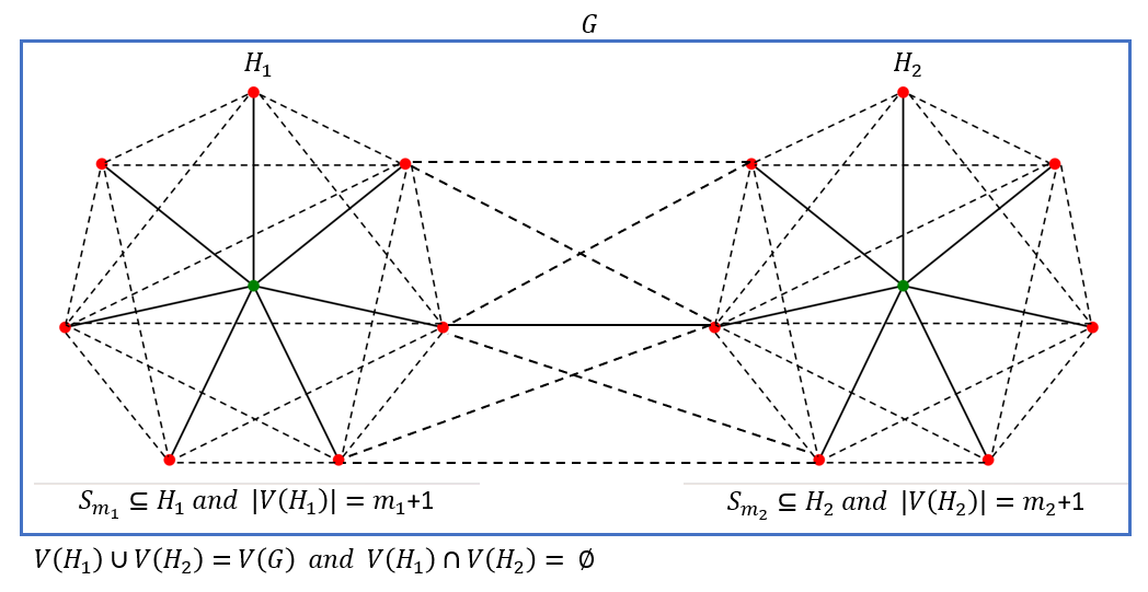
Figure 4: A graph $G$

In Figure 5, is shown an example where $|D_{h}|=4$, but the global domination number is 3.

Figure 5: A graph where the vertex set $\{u,v,v_{1},v_{2}\}$ is a possible solution given by Algorithm 2, however the vertex set $\{u,v_{1},v_{2}\}$ is a global dominating set of minimum cardinality.

The next proposition easily follows.

Proposition 17

Algorithm H1 runs in at most $|A_{0}|+|B_{0}|$ iterations and hence its time complexity is $O(n^{3})$.

6 Algorithm H2

Our next heuristic algorithm H2, at each iteration complements the current vertex set $D_{h}$ with two vertices, $v_{h}$ and $u_{h}$, defined (differently from the previous section) as follows: $v_{h}$ is a vertex dominating the maximum number of yet non-dominated vertices in graph $G$, i.e., it has the maximum number of the adjacent vertices among those who do not yet have a neighbor in set $D_{h}$. Likewise, vertex $u_{h}$ is one that dominates the maximum number of yet non-dominated vertices in graph $\overline{G}$, i.e., it has the maximum number of non-adjacent vertices among those that are not adjacent with a vertex in set $D_{h}$. In other words, $v_{h}\in V\setminus D_{h}$ is a vertex with

$$N_{V\setminus N[D_{h}]}[v_{h}]=\max_{v\in V\setminus D_{h}}N_{V\setminus N[D_{h}]}[v].$$

Likewise, $u_{h}\in V\setminus D_{h}$ is a vertex with

$$\overline{N}_{V\setminus\overline{N}[D_{h}]}[u_{h}]=\max_{v\in V\setminus D_{h}}\overline{N}_{V\setminus\overline{N}[D_{h}]}[v].$$

A detailed description of the algorithm follows.

Algorithm 3 H2

Input: A graph $G(V,E)$.

Output: A global dominating set $D_{h}$.

$D_{0}:=\emptyset$;

$C_{0}:=\emptyset$; { iterative step }

$h:=0$;

while  $D_{h}\cup C_{h}\neq V$  do

     $h:=h+1$;

     $v_{h}:=u_{h}:=NIL$;

     if  $D_{h}$ is not a dominant set of $G$  then

         $v_{h}$ := a vertex in set $V\setminus D$ such that $N_{V\setminus N[D]}[v]$ be maximum with $\overline{N}_{V\setminus\overline{N}[D]}[v]$ of maximum cardinality;

     end if

     $D_{h}:=D_{h-1}\cup\{v_{h}\}$;

     if  $D_{h}$ is not a dominant set of $\overline{G}$  then

         $u_{h}$ := a vertex in set $V\setminus D$ such that $\overline{N}_{V\setminus\overline{N}[D]}[u]$ be maximum with $N_{V\setminus N[D]}[u]$ of maximum cardinality;

         $D_{h}:=D_{h}\cup\{u_{h}\}$;

     end if

     $C_{h}:=N(D_{h})\cap\overline{N}(D_{h})$;

end while

In Figure 6 (a) and (b), we give examples when Algorithm H2 obtains an optimal and non-optimal, respectively, feasible solutions.

Figure 6: (a) The Petersen graph, where $\gamma_{g}(G)=4$ and Algorithm H2 delivers an optimal feasible solution $\{1,2,3,4\}$; (b) a graph where the black vertex set represents an optimal feasible solution, and $\{v_{1},v_{2},v_{3},v_{4}\}$ a global dominating set obtained by Algorithm H2.

We may easily observe that the upper bounds $U_{2}$ and $U_{1}$ introduced in Section 2 (Theorems 4 and 5) are attainable for example, for the complete graph with $n$ vertices $K_{n}$ and the Petersen graph depicted in Figure 6(a), respectively. At the same time, for both types of graphs, Algorithm H2 returns an optimal solution (see again Figure 6(a) illustrating the Petersen graph and the optimal solution generated by the algorithm for that graph).

Next, we define a wider family of graphs for which the heuristic is optimal. Let $G$ with $|V(G)|=n$ and $H_{i}$, $i=1,2,\dots,n$ be connected graphs, all of the order no smaller than two, and let $G^{\prime}=G\circ_{v_{i}}H_{i}$ be the graph composed of these $n+1$ graphs, in which every vertex from graph $G$ is associated with a specially determined vertex $v_{i}$ of graph $H_{i}$ (as we will see, we will choose vertex $v_{i}$ from a $\gamma(H_{i})$-set). Figure 7 illustrates an example of such a compouned graph, where every $H_{i}$ is the Petersen graph, where in Figure 8 $G$ is the line graph $P_{n}$. In Figure 9 we illustrate another such graph, where $H_{i}$s are different.

Figure 7: Graph $G^{\prime}=G\circ_{v}H$, where $H$ is a Petersen graph.

Proposition 18

Given graph $G^{\prime}=G\circ_{v_{i}}H_{i}$ with $|V(G)|=n\geq 2$ and $v_{i}\in\gamma(H_{i})$-set, $\gamma_{g}(G^{\prime})$-set is $\cup_{i=1}^{n}\gamma(H_{i})$-set.

Proof. As it is easy to see, $n\geq 2$ implies that any two $v_{i}$-type vertices form a dominating set of graph $\overline{G^{\prime}}$, whereas $\{v_{i}|i=\overline{1,n}\}$ form a dominating set of graph $G$ since $v_{i}\in\gamma(H_{i})$-set. Hence, $\bigcup\limits_{i=1}^{n}\gamma(H_{i})$-set is a global dominating set of $G^{\prime}$.

For example, if $H_{i}$s are the Petersen graphs, then by above proposition, $\gamma_{g}(G^{\prime})=3n$ (see Figure 7). If, in addition $G$ is $P_{n}$ or $C_{n}$ (the cycle graph of $n$ vertices), then Algorithm H2 will find an optimal solution for graph $G^{\prime}$ with $\gamma(G^{\prime})=3\gamma(H_{i})=9$, see Figure 8. Note that since $\gamma_{g}(G^{\prime})$-set and $\gamma(G^{\prime})$-set are identical, the lower bound from Theorem 2 is attained.

Figure 8: Graph $G^{\prime}=P_{3}\circ_{v}H$, where $H$ is a Petersen graph. The global domination number is 9 and Algorithm H2 obtain an optimal solution choosing the vertices in the shown order

The next theorem deals with a more general family of graphs:

Theorem 19

Let $H_{i}$, $i=\overline{1,n}$, be a connected graph of order $m_{i}+1$ containing the star graph $S_{m_{i}}$ as a subgraph, such that $m_{1}\geq m_{2}\geq\ldots\geq m_{i}\geq\ldots\geq m_{n-1}\geq m_{n}>\Delta(G)$. Let, further, $v_{i}$ be the center of graph $S_{m_{i}}$ (a vertex with maximum degree $m_{i}$ in that graph), and let $G$ be a connected graph of order $n$. Then Algorithm H2 finds an optimal solution for graph $G^{\prime}=G\circ_{v_{i}}H_{i}$.

Proof. Clearly, $\{v_{i}\}$ is a dominating set of graph $H_{i}$ and $\gamma_{g}(G^{\prime})$-set is $\cup_{i=1}^{n}\{v_{i}\}$ (see Proposition 18 and Figure 9). Since $\Delta(G)$ is less than all $m_{i}$, Algorithm H2 in the first iteration will select the two vertices of type $v_{i}$ with the highest degrees, that is, $\{v_{1},v_{2}\}$, that forms a dominating set of graph $\overline{G^{\prime}}$. In every following iteration $h=2,\dots,n-1$, Algorithm H2 adds vertex $v_{i+1}$ to the current solution and returns a global dominating set $D=\{v_{i}|i=\overline{i,n}\}$ at iteration $n-1$, which is optimal by Proposition 18.

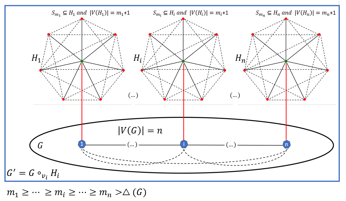
Figure 9: Graph $G^{\prime}=G\circ_{v_{i}}H_{i}$. The global domination number is $n$ and Algorithm H2 obtain an optimal solution choosing the green vertices.

7 Algorithm H3

In our last Algorithm H3, the vertex sets $D_{h}$, $A_{h}$, $B_{h}$ and $C_{h}$ and the initial iteration 0 with vertices $u$ and $v$ are defined as in Algorithm H1. The interactive parts of Algorithms H1 and H2 are combined as follows. If the condition $A_{h-1}=B_{h-1}=\emptyset$ (see Observation 14) is satisfied, then the algorithm halts at iteration $h\geq 1$. Otherwise, it determines vertices $v_{h},\;v_{h}^{\prime},\;u_{h}$:

• $v_{h}$ is a vertex in $V\setminus D_{h-1}$ with the maximum global active degree;

• $v_{h}^{\prime}\in V\setminus D_{h-1}$ is a vertex with $N_{V\setminus N[D_{h-1}]}[v_{h}^{\prime}]=\max_{v\in V\setminus D_{h-1}}N_{V\setminus N[D_{h-1}]}[v]$;

• $u_{h}\in V\setminus D_{h-1}$ is a vertex with $\overline{N}_{V\setminus\overline{N}[D_{h-1}]}[v_{h}]=\max_{v\in V\setminus D_{h-1}}\overline{N}_{V\setminus\overline{N}[D_{h-1}]}[v].$

Let

$$GAD(v_{h}^{\prime},u_{h})=|N_{A_{h-1}}[\{v_{h}^{\prime},u_{h}\}]\cup\overline{N}_{B_{h-1}}[\{v_{h}^{\prime},u_{h}\}]|.$$

If $GAD(v_{h})\geq GAD(v_{h}^{\prime},u_{h})/2$, then we let $D_{h}:=D_{h-1}\cup\{v_{h}\}$; otherwise, we let $D_{h}:=D_{h-1}\cup\{v_{h}^{\prime},u_{h}\}$. If $A_{h-1}=\emptyset$, vertex $v_{h}^{\prime}$ is not defined, and if $B_{h-1}=\emptyset$, vertex $u_{h}$ is not defined. The sets $A_{h}$, $B_{h}$ and $C_{h}$ are updated correspondingly. A detailed description is given below.

Algorithm 4 H3

Input: A graph $G(V,E)$.

Output: A global dominating set $D_{h}$.

$h:=0$;

$\{u,v\}$ := two vertex with the largest possible cardinality of the set

$(N[u]\cup N[v])\setminus(N[u]\cap N[v])$;

$D_{0}:=\{u,v\}$;

$C_{0}:=(N[u]\cup N[v])\setminus(N[u]\cap N[v])$;

$A_{0}:=V\setminus(N[u]\cup N[v])$;

$B_{0}:=V\setminus(D_{0}\cup C_{0}\cup A_{0})$; { iterative step }

while  $A_{h}\neq\emptyset\vee B_{h}\neq\emptyset$  do

     $h:=h+1$;

     $v_{h}$ := a vertex in the set $V\setminus D_{h-1}$ with the maximum $GAD(v_{h})$;

     if  $A_{h}\neq\emptyset$  then

         $v_{h}^{\prime}$ := a vertex in the set $V\setminus D_{h-1}$ such that $N_{V\setminus N[D_{h-1}]}[v_{h}^{\prime}]$ be maximum;

     end if

     if  $B_{h}\neq\emptyset$  then

         $u_{h}$ := a vertex in the set $V\setminus D_{h-1}$ such that $\overline{N}_{V\setminus\overline{N}[D_{h-1}]}[u_{h}]$ be maximum;

     end if

     if  $GAD(v_{h})\geq GAD(v_{h}^{\prime},u_{h})/2$ then

         $D_{h}:=D_{h-1}\cup\{v_{h}\}$;

         $C_{h}:=C_{h-1}\cup N_{A_{h-1}}(v_{h})\cup\overline{N}_{B_{h-1}}(v_{h})$;

         $A_{h}:=A_{h-1}\setminus N_{A_{h-1}}(v_{h})$;

         $B_{h}:=B_{h-1}\setminus\overline{N}_{B_{h-1}}(v_{h})$;

     else

         $D_{h}:=D_{h-1}\cup\{v_{h}^{\prime},u_{h}\}$;

         $C_{h}:=C_{h-1}\cup N_{A_{h-1}}(v_{h}^{\prime},u_{h})\cup\overline{N}_{B_{h-1}}(v_{h}^{\prime},u_{h})$;

         $A_{h}:=A_{h-1}\setminus N_{A_{h-1}}(v_{h}^{\prime},u_{h})$;

         $B_{h}:=B_{h-1}\setminus\overline{N}_{B_{h-1}}(v_{h}^{\prime},u_{h})$;

     end if

end while

8 Procedure Purify

Purification procedures have been successfully used for the reduction of the set of vertices in a given dominating set. Below we apply similar kind of a reduction to any given global dominating set. We need the following definition.

Let $D^{*}=\{v_{1},...,v_{p}\}$ be a formed global dominating set, the vertices being included in this particular order into that set. We define the purified set $D$ as follows. Initially, $D:=D^{*}$; iteratively, for $i=p,...,1$: if $pn(v_{i},D,G)=\emptyset$ and $pn(v_{i},D,\overline{G})=\emptyset$ then we let $D:=D\setminus\{v_{i}\}$, i.e. we purify vertex $v_{i}$.

The so formed set $D$ is a minimal global dominating set for graph $G$ since, by the construction, by eliminating any vertex, the resultant set will not globally dominate the private neighbors of that vertex. It is easy to see that Procedure Purify can be implemented in time $O(pn^{2})=O(n^{3})$.

9 Experimental Results

In this section we describe our computation experiments. We implemented our algorithms in C++ using Windows 10 operative system for 64 bits on a personal computer with Intel Core i7-9750H (2.6 GHz) and 16 GB of RAM DDR4. We tested our algorithms for the benchmark problem instances from Parra Inza [2023], 2284 instances in total. First, we describe the results concerning our exact algorithms and then we deal with our heuristics. We analyze the performance of these heuristics based, in particular, on the optimal solutions obtained by our exact methods and known upper and lower bounds.

The performance of our exact algorithms. For 25 middle-sized middle-dense instances, in at most four iterations an optimal solution was found by both BGDS and the ILP method. Figure 10 illustrates how the lower and upper bounds were updated during the execution of the algorithm and how the cardinality of the formed dominating sets was iteratively reduced.

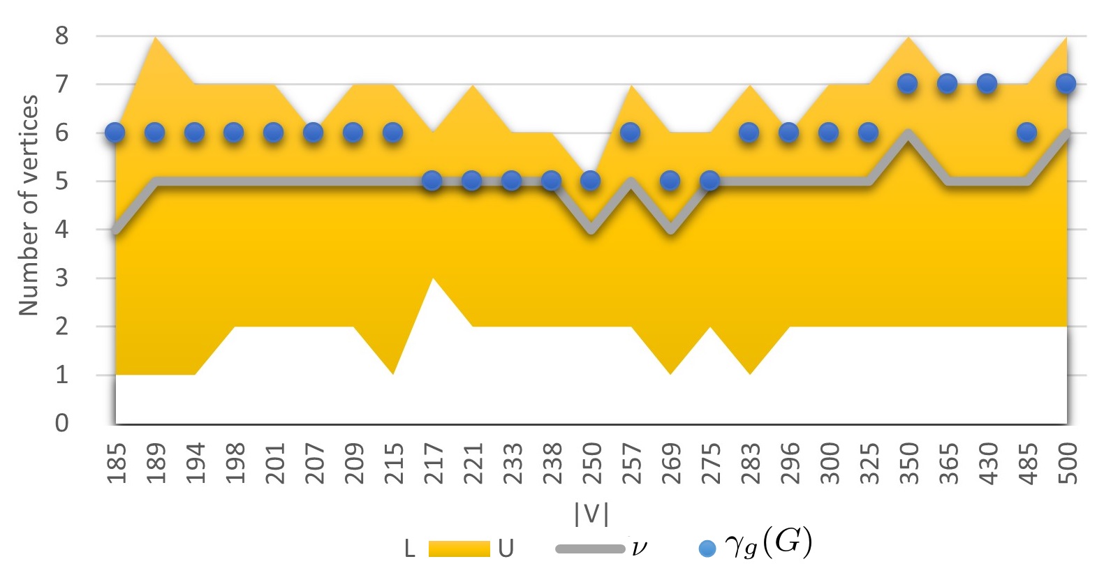
(a) Iteration 1

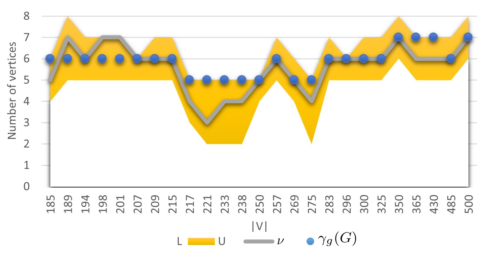
(b) Iteration 2

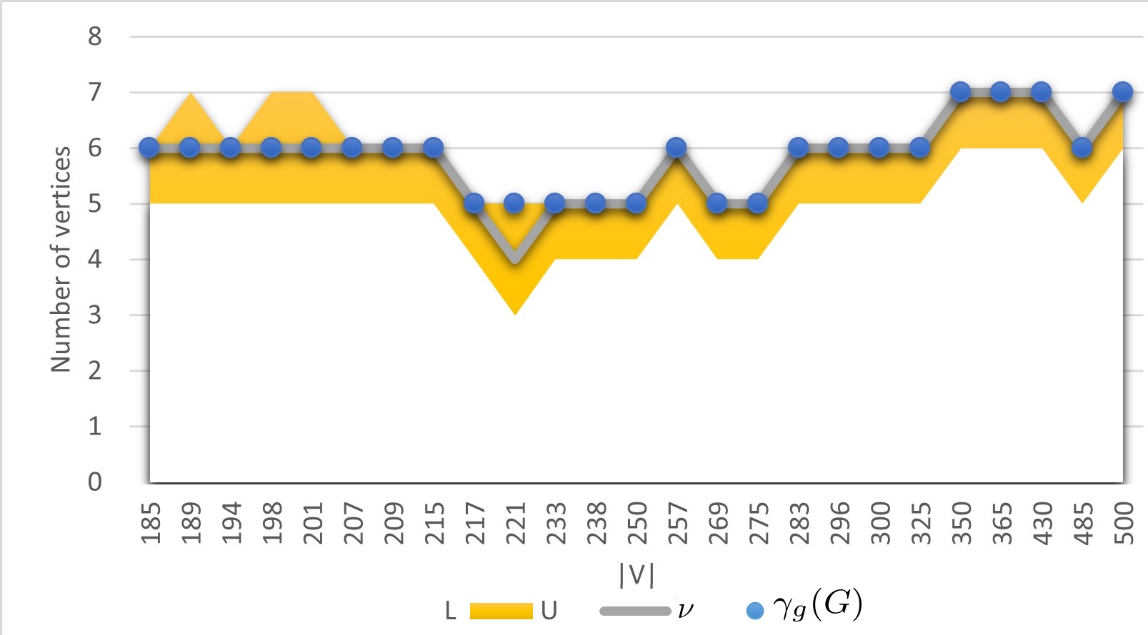
(c) Iteration 3

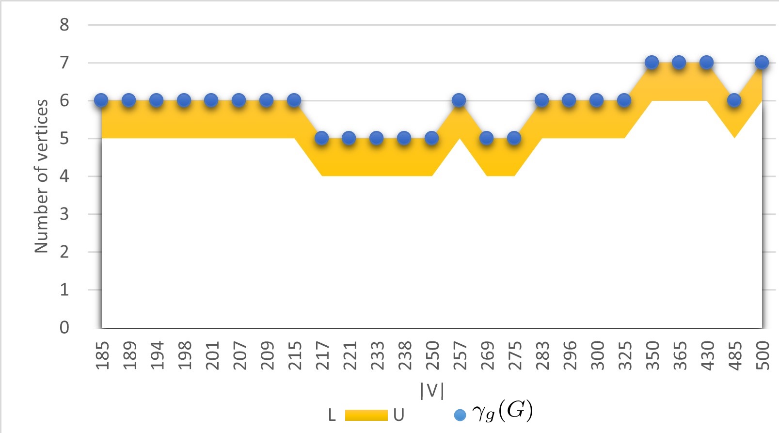
(d) Iteration 4

Figure 10: Vertical lines represent lower and upper bounds and the cardinalities of the corresponding solutions, and horizontal lines represent the size of the corresponding instances. Ranges for lower and upper bounds are delineated by yellow regions, where the gray lines show the current value of $\nu$; blue circles represent $\gamma_{g}(G)$

Table LABEL:tabla8 presents the results for small-sized graphs with the density of approximately 0.2 for both exact algorithms. For these instances, ILP formulation gave better results (due to small amount of variables in linear programs).

Table 1: The results for the graphs with density $\approx 0.2$.

No.	$|V(G)|$	$|E(G)|$	Time		Lower Bounds				$\gamma_{g}(G)$	U
			ILP	BGDS	$\frac{n}{\Delta(G)+1}$	$\frac{d+1}{3}$	$\frac{2r}{3}$	$|Supp(G)|$
1	50	286	0.18	1.79	2	1	1	2	7	7
2	60	357	0.13	4.16	2	1	1	1	6	7
3	70	524	0.16	7.44	2	1	1	1	7	8
4	80	678	0.14	11.93	2	1	1	1	6	6
5	90	842	0.18	384.92	3	1	1	1	8	9
6	100	1031	0.23	794.41	2	1	1	2	7	7
7	101	1051	1.31	811.32	3	1	1	1	8	8
8	106	1154	1.57	973.85	2	1	1	1	7	8
9	113	1306	1.34	1384.32	3	1	1	1	7	7
10	117	1398	2.73	3474.51	3	1	1	2	8	9
11	121	1493	3.11	2586.79	3	1	1	1	7	7

For middle-dense graphs, where exact algorithms succeeded to halt with an optimal solution, Algorithm BGDS showed better performance for the graphs with more than 230 vertices, where ILP formulation gave better results for smaller sized graphs (see Table LABEL:tabla9 and Figure 11 below).

Table 2: The results for the graphs with density $\approx 0.5$.

No.	$|V(G)|$	$|E(G)|$	Time		Lower Bounds				$\gamma_{g}(G)$	U
			ILP	BGDS	$\frac{n}{\Delta(G)+1}$	$\frac{d+1}{3}$	$\frac{2r}{3}$	$|Supp(G)|$
1	185	6849	3.25	23.63	1	1	1	1	6	6
2	189	7147	3.87	22.55	1	1	1	1	6	8
3	194	7529	4.09	28.29	1	1	1	1	6	7
4	198	7842	3.71	31.53	2	1	1	1	6	7
5	201	8081	4.82	31.03	2	1	1	2	6	7
6	207	8569	5.28	33.91	2	1	1	1	6	6
7	209	8735	7.41	35.65	1	2	1	1	6	7
8	215	9243	12.25	41.79	1	1	1	1	6	7
9	217	9415	19.16	32.18	1	1	1	3	5	6
10	221	9765	24.73	39.91	2	1	1	1	5	7
11	233	10852	32.74	27.83	2	1	1	1	5	6
12	238	11322	51.49	45.56	2	1	1	1	5	6
13	250	12491	86.09	74.19	1	2	1	1	5	5
14	257	13199	128.43	94.89	2	1	1	1	6	7
15	269	14459	134.03	102.60	1	1	1	1	5	6
16	275	15111	583.66	124.46	2	1	1	1	5	6
17	283	16002	1166.80	436.23	1	1	1	1	6	7
18	296	17505	5837.52	385.61	2	1	1	1	6	6
19	300	17981	6418.32	405.03	2	1	1	1	6	7
20	325	24896	7002.01	571.27	1	2	1	1	6	7
21	350	27495	7854.36	3057.62	2	2	1	1	7	8
22	365	31606	8153.24	6686.34	2	1	1	1	7	7
23	430	44216	10121.83	7001.24	1	2	1	1	7	7
24	485	56536	11936.22	1484.51	1	2	1	1	6	7
25	500	60158	12351.49	4525.39	2	1	1	1	7	8

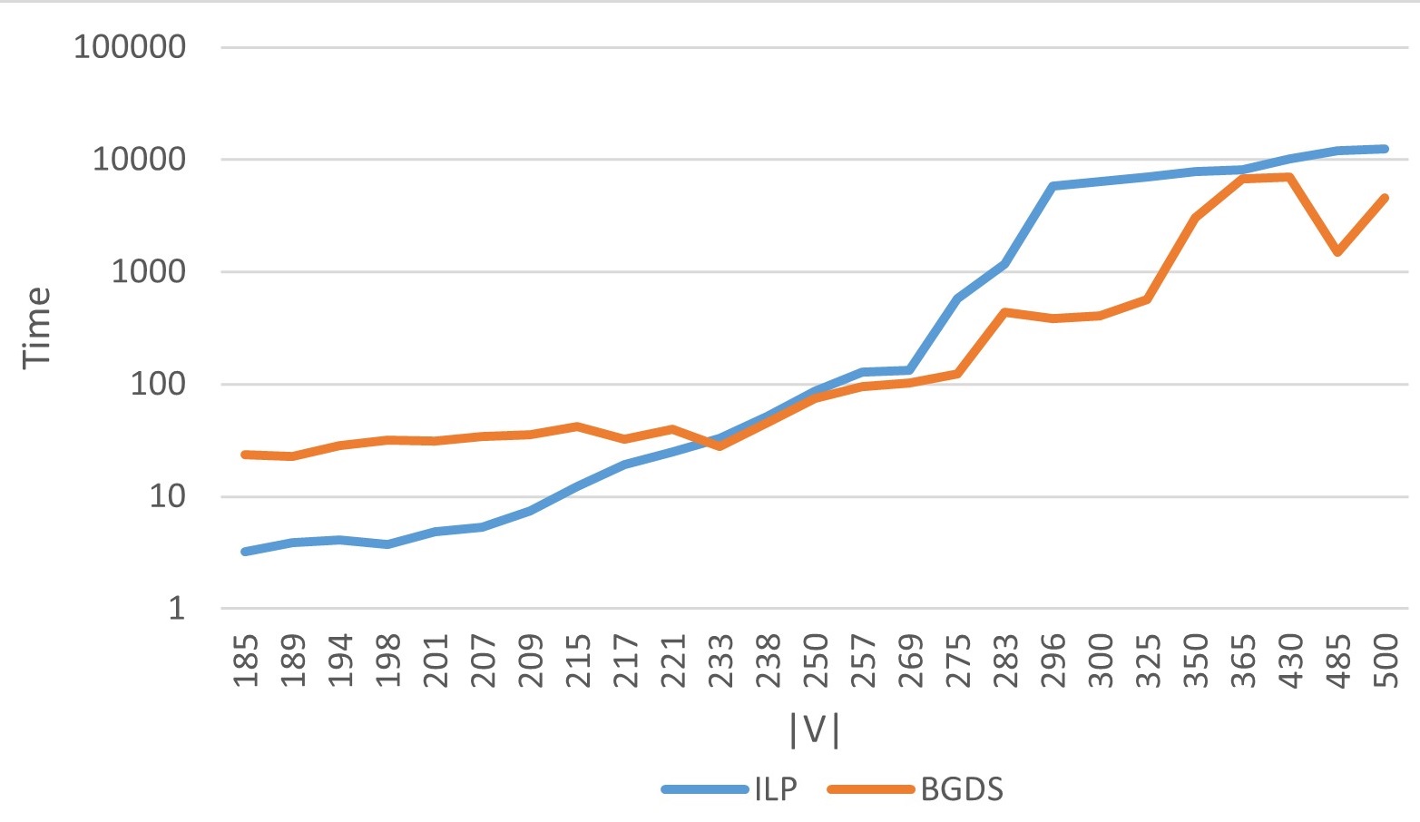
Figure 11: BGDS vs. ILP for the graphs with density $\approx 0.5$ (logarithmic scale was applied).

Table LABEL:tabla3 presents results for larger instances up to 1098 vertices with high density ($\approx 0.8$). Both exact algorithm completed within 120 minutes for the largest instances. For these dense quasi complete graphs $\gamma_{g}(G)$ turned out to be very small (ranging from 4 to 7), where ILP formulation resulted in smaller execution times (see Figure 12).

Table 3: Results for the graphs with density $\approx 0.8$

No.	$|V(G)|$	$|E(G)|$	Time		Lower Bounds				$\gamma_{g}(G)$	U
			ILP	BGDS	$\frac{n}{\Delta(G)+1}$	$\frac{d+1}{3}$	$\frac{2r}{3}$	$|Supp(G)|$
1	250	23169	10.34	28.61	1	2	2	2	5	5
2	302	38543	16.89	24.97	1	2	2	2	4	5
3	352	46953	22.39	103.23	1	2	2	2	5	6
4	420	67432	23.09	205.13	1	2	2	2	5	5
5	474	97121	20.11	113.59	1	2	2	2	4	5
6	518	116381	32.56	160.37	1	2	2	2	4	5
7	580	130202	37.67	746.51	1	2	2	2	5	6
8	634	175537	33.93	410.16	1	2	2	2	4	5
9	712	222137	39.85	646.24	1	2	2	2	4	5
10	746	244124	44.08	753.398	1	2	2	2	4	5
11	816	260190	47.24	2604.72	1	2	2	2	5	6
12	892	350495	41.63	3017.06	1	2	2	2	5	5
13	932	382996	47.28	1805.78	1	2	2	2	4	5
14	970	415180	43.83	4186.27	1	2	2	2	5	5
15	972	416905	37.55	4360.8	1	2	2	2	5	5
16	1014	454116	40.84	5136.9	1	2	2	2	5	5
17	1036	474219	48.64	5341.2	1	2	2	2	5	5
18	1042	426451	44.52	6742.94	1	2	2	2	5	6
19	1064	500420	40.21	6224.74	1	2	2	2	5	5
20	1068	504205	41.84	3173.52	1	2	2	2	4	5
21	1080	515722	44.24	6698.43	1	2	2	2	5	5
22	1096	531243	52.96	7010.88	1	2	2	2	5	5
23	1098	533220	51.51	7246.31	1	2	2	2	5	5

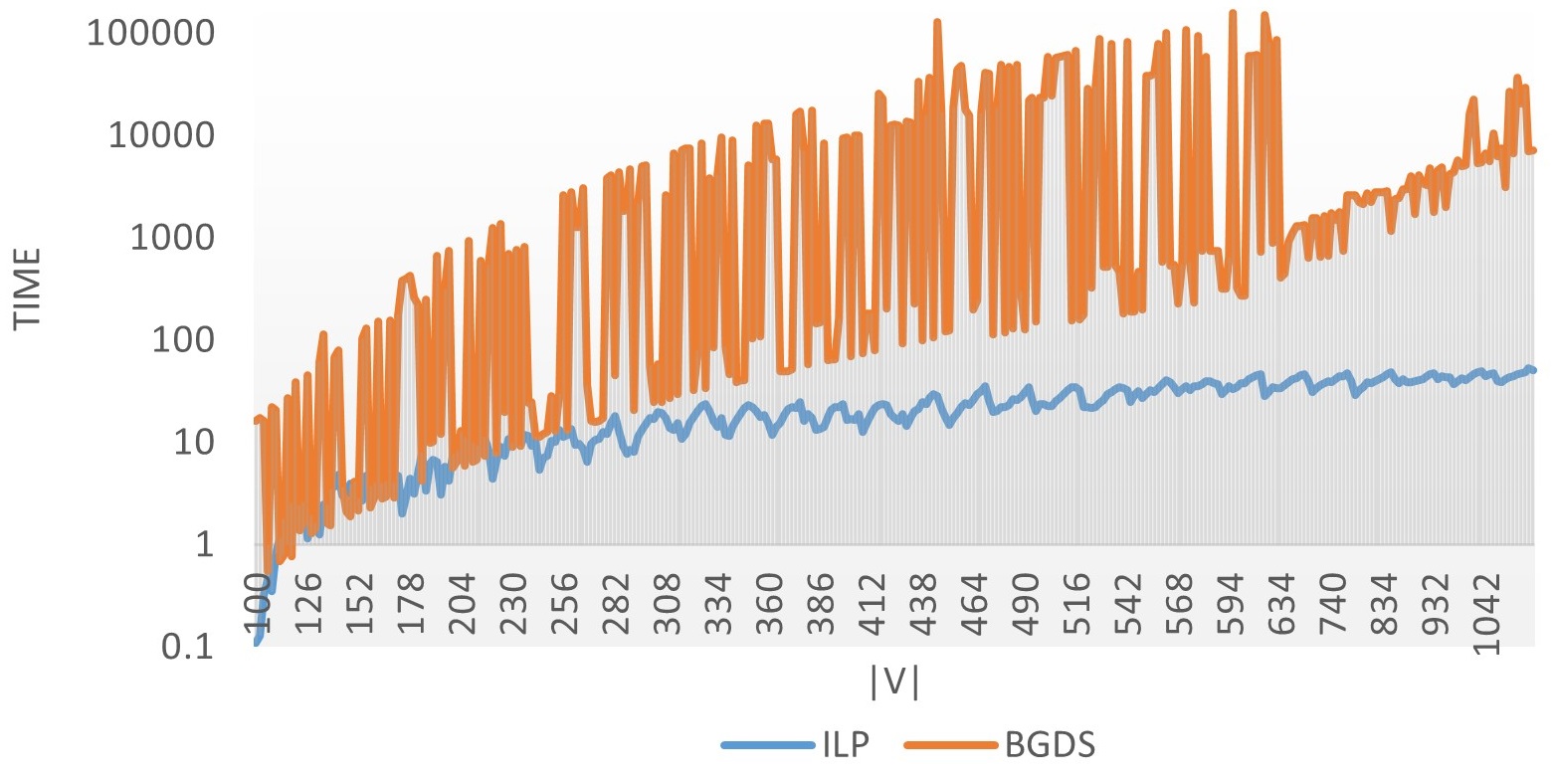
Figure 12: BGDS vs. ILP for dense graphs (logarithmic scale was applied).

The performance of the heuristic algorithms. In Figure 13 we compare the quality of the best solution generated by our heuristic algorithms vs optimal values obtained by our exact algorithms for the large-sized instances with up to 1098 vertices. In this figure, blue nodes represent optimal solutions, and red squares in black frames represent a best solution obtained by our heuristics. As we can see, the heuristics found an optimal solution in $52.03\%$ of the instances, whereas, among the instances where the optimum was not found, the average approximation error was $1.07$.

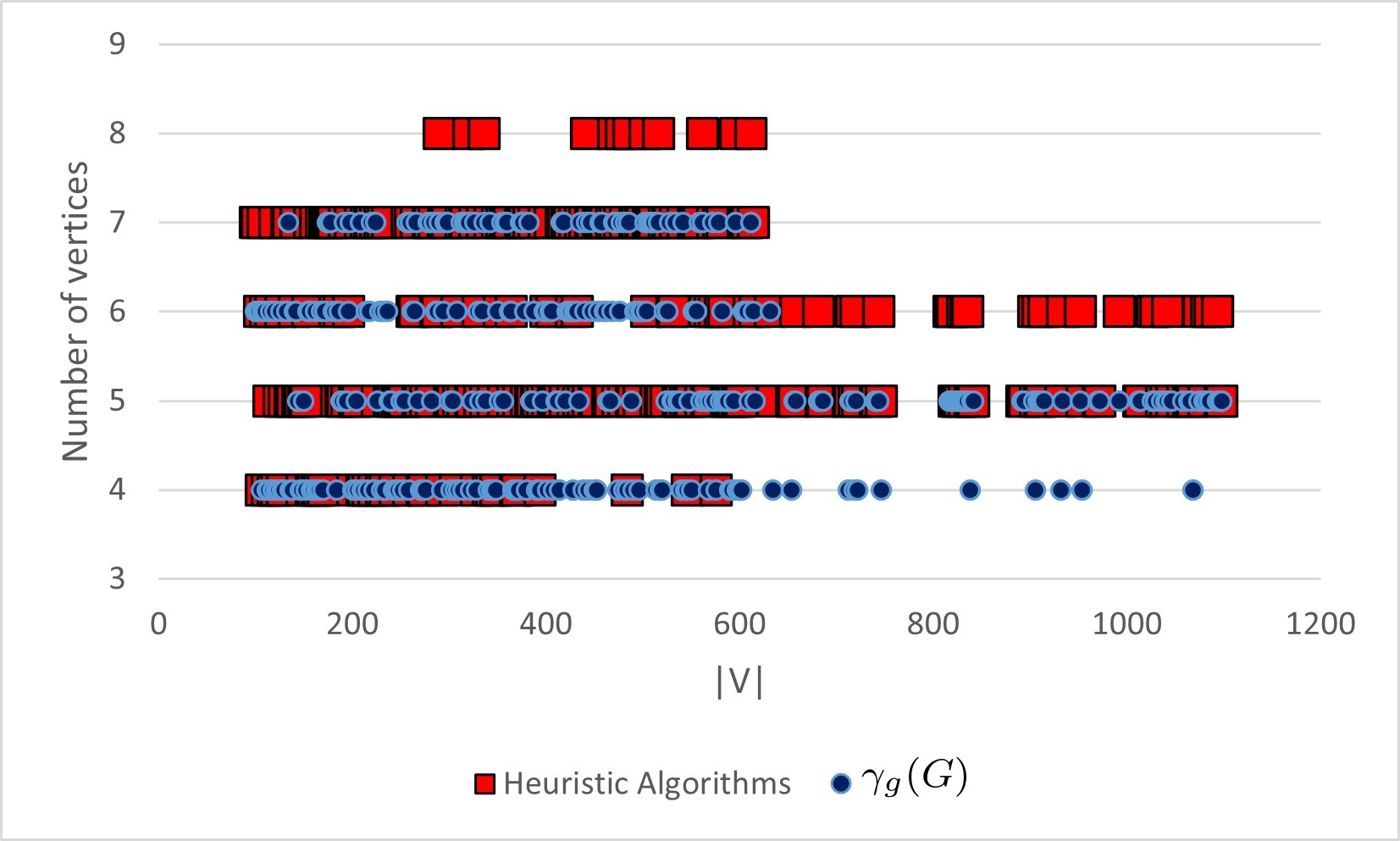
Figure 13: $\gamma_{g}(G)$ vs. approximation results.

The above reported results of our heuristics include the purification stage. In fact, the purification process turned out to be efficient, in practice, as illustrated in Tables LABEL:table1 and LABEL:table6, in which the values of the corresponding lower and upper bounds $L$ and $U$ are also shown; $|D|$ and $|D^{*}|$, respectively, stand for the number of vertices in the global dominant set obtained before and after, respectively, purification.

Table 4: Results of Algorithm H1 and H2 for the randomly generated graphs.

No.	$|V|$	$|E|$	L	Algorithm H1				Algorithm H2				U
				Time(s)	$|D_{H1}|$	$|D_{H1}^{*}|$	% Purified	Time(s)	$|D_{H2}|$	$|D_{H2}^{*}|$	% Purified
1	7300	7311	2663	2794.67	3344	2706	19.08	567.73	3161	2706	14.39	6843
2	7350	7474	2621	2839.76	3365	2726	18.99	578.91	3177	2722	14.32	6890
3	7400	7474	2677	2949.72	3392	2743	19.13	591.42	3202	2740	14.43	6937
4	7450	7497	2695	2996.26	3399	2756	18.92	607.24	3218	2755	14.39	6984
5	7500	7535	2762	3077.71	3427	2822	17.65	615.30	3270	2822	13.70	7031
6	7550	7557	2775	3192.53	3478	2832	18.57	628.30	3301	2831	14.24	7078
7	7600	7734	2729	3223.23	3425	2831	17.34	642.02	3277	2830	13.64	7125
8	7650	7696	2797	3269.30	3490	2855	18.19	658.27	3336	2851	14.54	7171
9	7700	7716	2803	3325.65	3521	2862	18.72	703.98	3334	2860	14.22	7218
10	7750	7806	2807	3370.84	3534	2886	18.34	684.13	3344	2882	13.82	7265
11	7800	7804	2879	3428.42	3571	2932	17.89	704.58	3397	2932	13.69	7312
12	7850	7884	2851	3499.23	3556	2913	18.08	705.05	3363	2910	13.47	7359
13	7900	7932	2889	3584.14	3588	2947	17.87	727.14	3416	2946	13.76	7406
14	7950	7982	2949	6376.02	3641	3004	17.50	753.24	3481	3004	13.70	7453
15	8000	8126	2882	6828.32	3624	2966	18.16	758.84	3469	2964	14.56	7500
16	9150	10443603	3	6762.49	21	20	4.76	17.71	22	19	13.64	6485
17	9200	10558172	3	6887.40	21	20	4.76	18.11	22	19	13.64	6489
18	9250	10673366	3	7020.20	20	19	5.00	17.71	21	19	9.52	6523
19	9300	14357729	3	8222.71	20	18	10.00	21.33	21	17	19.05	5703
20	9350	14540834	2	8380.73	16	15	6.25	18.87	18	15	16.67	5700
21	9400	11001589	3	7428.46	23	21	8.70	21.87	25	21	16.00	6579
22	9450	14825554	3	8755.81	19	17	10.53	20.95	20	16	20.00	5742
23	9500	14983162	3	8857.65	20	18	10.00	25.09	20	16	20.00	5791
24	9550	15141604	3	8974.30	20	18	10.00	26.14	24	18	25.00	5773
25	9600	15329626	2	9114.64	16	15	6.25	19.76	18	16	11.11	5800
26	9650	15460987	3	10186.50	20	18	10.00	22.17	20	17	15.00	5790
27	9700	15621929	3	10488.80	19	17	10.53	22.48	20	16	20.00	5832
28	9750	15812901	2	10639.20	16	15	6.25	19.54	17	15	11.76	5842
29	9800	11959739	3	12332.80	23	21	8.70	26.78	28	21	25.00	6805
30	12600	39630183	2	30335.40	12	11	8.33	37.34	12	11	8.33	5406
31	12650	39945571	2	30143.80	13	12	7.69	44.06	14	11	21.43	5419
32	12700	40262208	2	35540.20	13	12	7.69	43.48	14	11	21.43	5436
33	12750	40580096	2	40648.00	13	12	7.69	44.04	14	11	21.43	5437
34	12800	40841707	3	36502.20	15	13	13.33	53.28	16	13	18.75	5438
35	12850	41219621	2	37844.20	13	12	7.69	41.89	13	12	7.69	5450
36	12900	41541258	2	39178.50	12	11	8.33	38.03	12	11	8.33	5448
37	12950	41864146	2	41767.80	12	11	8.33	37.53	12	11	8.33	5448
38	13000	42188283	2	43198.60	12	11	8.33	41.69	13	10	23.08	5433
39	13100	42840308	2	42710.00	12	11	8.33	42.70	13	10	23.08	5446
40	13150	43168196	2	40698.00	12	11	8.33	41.15	12	11	8.33	5442

In Table LABEL:table2 we compare the quality of the solutions obtained by Algorithms H1 and H2 before the purification stage, represented by the parameters $|D_{H1}|$ and $|D_{H2}|$, respectively.

Table 5: Comparative analysis of heuristics H1 and H2 before the purification

	Instances	%
$|D_{H1}|=|D_{H2}|$	781	34.19
$|D_{H1}|>|D_{H2}|$	365	15.98
$|D_{H1}|<|D_{H2}|$	1138	49.83

The tables below present comparative analysis of the heuristics after the purification. As we can see, in 100% of the instances, the solutions delivered by Algorithm H2 were purified. Algorithm H1 delivered minimal global dominating sets for 7.48% of the instances (note that a minimal dominating set cannot be purified). Both algorithms halted within a few seconds for the instances with up to 1000 vertices. Algorithm H2 turned out to be faster, delivering solutions within a few seconds for most of the instances, while for the largest instance with 14 100 vertices, it hated within 50 seconds. Algorithm H1 took about 11 hours for this instance. In average, among the instances that were solved by the both algorithms, Algorithm H2 was about 88 times faster.

Table 6: Comparative analysis of heuristics H1 and H2 after the purification

	Instances	%
$|D_{H1}^{*}|=|D_{H2}^{*}|$	1286	56.31
$|D_{H1}^{*}|>|D_{H2}^{*}|$	905	39.62
$|D_{H1}^{*}|<|D_{H2}^{*}|$	93	4.07

The observed drastic difference in the execution times of Algorithms H1 and H2 can be reduced by simply omitting the initial iteration $h=0$ of Algorithms H2, the most time consuming part of that algorithm. The execution time of the modified Algorithm H1 in average, has reduced almost 160 time. As to the quality of the solutions, the original version gave better solutions in 18.43% of the tested instances. Table LABEL:table4 (Table LABEL:table5, respectively) gives more detailed comparisons before (after, respectively) application of the purification procedure; $|D_{H1}|$, $|D_{H1_{mod}}|$, $|D^{*}_{H1}|$, $|D^{*}_{H1_{mod}}|$ stand for the cardinality of the corresponding global dominating sets, before and after the purification.

Table 7: Comparative analysis of the two versions of heuristic H1 before the purification

	Instances	%
$|D_{H1}|=|D_{H1_{mod}}|$	1558	68.21
$|D_{H1}|>|D_{H1_{mod}}|$	190	8.32
$|D_{H1}|<|D_{H1_{mod}}|$	536	23.47

Table 8: Comparative analysis of the two versions of heuristic H1 after the purification

	Instances	%
$|D_{H1}^{*}|=|D_{H1_{mod}}^{*}|$	1660	72.68
$|D_{H1}^{*}|>|D_{H1_{mod}}^{*}|$	203	8.89
$|D_{H1}^{*}|<|D_{H1_{mod}}^{*}|$	421	18.43

Recall that Algorithms H3 uses Algorithm H1 as a subroutine. Above we considered a modification of the latter algorithm, which resulted in a much faster performance but a bit worst solution quality. We carried out similar modifications in Algorithm H3, and we got similar outcome. Table LABEL:table6 gives related results for about 40 selected instances. Among the instances that were solved by Algorithm H3 and its modification, in average, the modified heuristic was about 83 times faster. This drastic difference was achieved by just eliminating the initial iteration of Algorithm H3 (H1). Compared to Algorithm H2, in average, modified Algorithm H3 was about $5$ times slower. The global dominating sets delivered by Algorithm H3 and its modification were purified in 93.15% and 93.22% of the instances, respectively (with an average of approximately 30 reduced vertices). Tables LABEL:table8 and LABEL:table9 give a comparative analysis of the two versions of the heuristic before and after the purification stage, respectively.

Table 9: Results for the two versions of heuristic H3 for 41 randomly generated instances

No.	$|V|$	$|E|$	L	Algorithm H3				Modified Algorithm H3				U
				Time(s)	$|D_{H3}|$	$|D_{H3}^{*}|$	% Purified	Time(s)	$|D_{H3_{mod}}|$	$|D_{H3_{mod}}^{*}|$	% Purified
1	7300	7311	2663	3934.11	3158	2706	14.31	1118.17	3158	2706	14.31	6843
2	7350	7474	2621	4262.89	3174	2722	14.24	1114.77	3174	2722	14.24	6890
3	7400	7474	2677	4306.95	3200	2740	14.38	1150.65	3200	2740	14.38	6937
4	7450	7497	2695	4731	3217	2755	14.36	1170.54	3217	2755	14.36	6984
5	7500	7535	2762	4862.41	3270	2822	13.70	1209.28	3270	2822	13.70	7031
6	7550	7557	2775	5244.28	3298	2831	14.16	1242.61	3298	2831	14.16	7078
7	7600	7734	2729	4510.99	3271	2829	13.51	1261.24	3271	2829	13.51	7125
8	7650	7696	2797	3370.89	3331	2851	14.41	1287.06	3331	2851	14.41	7171
9	7700	7716	2803	3418.88	3331	2860	14.14	1301.44	3331	2860	14.14	7218
10	7750	7806	2807	3544.64	3341	2882	13.74	1328.39	3342	2882	13.76	7265
11	7800	7804	2879	3586.43	3395	2932	13.64	1359.95	3395	2932	13.64	7312
12	7850	7884	2851	3645.01	3359	2910	13.37	1395.35	3359	2910	13.37	7359
13	7900	7932	2889	3708.27	3415	2946	13.73	1436.03	3415	2946	13.73	7406
14	7950	7982	2949	6423.91	3479	3004	13.65	1710.06	3479	3004	13.65	7453
15	8000	8126	2882	6742.18	3466	2964	14.48	1762.53	3466	2964	14.48	7500
16	9150	10443603	3	8849.74	21	20	4.76	24.7761	21	20	4.76	6485
17	9200	10558172	3	8219.12	21	20	4.76	24.461	21	20	4.76	6489
18	9250	10673366	3	8367.25	20	19	5.00	23.889	20	19	5.00	6523
19	9300	14357729	3	9683.22	20	18	10.00	27.0218	19	17	10.53	5703
20	9350	14540834	2	9899.63	16	15	6.25	24.9821	17	16	5.88	5700
21	9400	11001589	3	8808.05	23	21	8.70	27.4256	24	22	8.33	6579
22	9450	14825554	3	10319.8	19	17	10.53	27.8673	19	17	10.53	5742
23	9500	14983162	3	10548.7	20	18	10.00	27.7427	19	17	10.53	5791
24	9550	15141604	3	10751.4	20	18	10.00	29.1597	20	18	10.00	5773
25	9600	15329626	2	10890.4	16	15	6.25	28.2489	17	16	5.88	5800
26	9650	15460987	3	10941.8	20	18	10.00	29.9306	20	18	10.00	5790
27	9700	15621929	3	15073.5	19	17	10.53	31.4752	19	17	10.53	5832
28	9750	15812901	2	15339.3	16	15	6.25	28.8936	16	15	6.25	5842
29	9800	11959739	3	13978.7	23	21	8.70	31.5612	23	21	8.70	6805
30	12600	39630183	2	25428.1	12	11	8.33	38.1663	13	11	15.38	5406
31	12650	39945571	2	25952.5	13	12	7.69	38.9686	13	12	7.69	5419
32	12700	40262208	2	26387.9	13	12	7.69	36.3431	12	11	8.33	5436
33	12750	40580096	2	26763.6	13	12	7.69	44.107	12	11	8.33	5437
34	12800	40841707	3	31395	15	13	13.33	47.6085	16	14	12.50	5438
35	12850	41219621	2	31919.1	13	12	7.69	39.0515	12	11	8.33	5450
36	12900	41541258	2	32506.9	12	11	8.33	44.6907	13	12	7.69	5448
37	12950	41864146	2	34730.8	12	11	8.33	41.749	13	12	7.69	5448
38	13000	42188283	2	33157.2	12	11	8.33	39.7126	12	11	8.33	5433
39	13050	42455020	3	33496.8	15	13	13.33	47.6886	15	13	13.33	5450
40	13100	42840308	2	33583.9	12	11	8.33	39.2545	12	11	8.33	5446
41	13150	43168196	2	34047	12	11	8.33	39.0421	12	11	8.33	5442

Table 10: Comparative analysis of the two versions of heuristic H3 before the purification

	Instances	%
$|D_{H3}|=|D_{H3_{mod}}|$	1630	71.36
$|D_{H3}|>|D_{H3_{mod}}|$	179	7.84
$|D_{H3}|<|D_{H3_{mod}}|$	475	20.80

Table 11: Comparative analysis of the two versions of heuristic H3 after the purification

	Instances	%
$|D_{H3}^{*}|=|D_{H3_{mod}}^{*}|$	1686	73.82
$|D_{H3}^{*}|>|D_{H3_{mod}}^{*}|$	189	8.27
$|D_{H3}^{*}|<|D_{H3_{mod}}^{*}|$	409	17.91

Summary. We summarize the obtained results for our heuristics. Before the application of the purification procedure, solutions with equal cardinality were obtained in 31% of the analyzed instances. For the remaining instances, Algorithms H1, H2, and H3 obtained the best solutions in 70.54%, 8.69%, and 20.77% of the tested instances, respectively. When applying the purification procedure to the solutions delivered by Algorithm H2, the corresponding purified solutions were better than ones constructed by Algorithms H1 and H3. In average, the purification procedure reduced the size of the solutions delivered by Algorithms H1, H2, and H3 by 16.03%, 21.58% and 15.34%, respectively, see Table LABEL:table7 for a detailed comparative analysis.

Table 12: Comparative analysis of heuristics H1,H2 and H3 after the purification

	Instances	%
All	1233	53.98
H1	121	5.30
H2	887	38.84
H3	43	1.88

Comparing the size of the best obtained dominant sets with the upper bound $U$, $\min\{|D_{H1}^{*}|,|D_{H2}^{*}|,|D_{H3}^{*}|\}$ represents about $10\%$ of $U$ in average, i.e., an improvement of 90% over this upper bound. The lower bound $L$ represents, in average, $1/3$ of the cardinality of the obtained solutions. The complete experimental data can be found at Parra Inza [2023].

10 Conclusions

We proposed the first exact and approximation algorithms for the classical global domination problem. The exact algorithms were able to solve the existing benchmark instances with up to 1098 vertices, while the heuristics found high-quality solutions for the largest existing benchmark instances with up to 14 000 vertices. We showed that the global domination problem remains $NP$-hard for quite particular families of graphs and gave some families of graphs where our heuristics find an optimal solution. As to the future work, we believe that our line of research can be extended for more complex domination problems.

Conflict of interest

The authors declare there is no conflict of interest.

References

- Abu-Khzam & Lamaa [2018] Abu-Khzam, F. N., & Lamaa, K. (2018). Efficient heuristic algorithms for positive-influence dominating set in social networks. In IEEE INFOCOM 2018-IEEE Conference on Computer Communications Workshops (INFOCOM WKSHPS) (pp. 610–615). IEEE. doi:https://doi.org/10.1109/INFCOMW.2018.8406851.
- Bertossi [1984] Bertossi, A. A. (1984). Dominating sets for split and bipartite graphs. Information processing letters, 19, 37–40. doi:https://doi.org/10.1016/0020-0190(84)90126-1.
- Brigham & Dutton [1990] Brigham, R. C., & Dutton, R. D. (1990). Factor domination in graphs. Discrete Mathematics, 86, 127–136. doi:https://doi.org/10.1016/0012-365X(90)90355-L.
- Colombi et al. [2017] Colombi, M., Mansini, R., & Savelsbergh, M. (2017). The generalized independent set problem: Polyhedral analysis and solution approaches. European Journal of Operational Research, 260, 41–55. doi:https://doi.org/10.1016/j.ejor.2016.11.050.
- Desormeaux et al. [2015] Desormeaux, W. J., Gibson, P. E., & Haynes, T. W. (2015). Bounds on the global domination number. Quaestiones Mathematicae, 38, 563–572. doi:https://doi.org/10.2989/16073606.2014.981728.
- Doreian & Conti [2012] Doreian, P., & Conti, N. (2012). Social context, spatial structure and social network structure. Social networks, 34, 32–46. doi:https://doi.org/10.1016/j.socnet.2010.09.002.
- Enciso & Dutton [2008] Enciso, R. I., & Dutton, R. D. (2008). Global domination in planar graphs. J. Combin. Math. Combin. Comput, 66, 273–278. URL: https://citeseerx.ist.psu.edu/viewdoc/summary?doi=10.1.1.535.9636.
- Foldes & Hammer [1977] Foldes, S., & Hammer, P. L. (1977). Split graphs having dilworth number two. Canadian Journal of Mathematics, 29, 666–672. doi:https://doi.org/10.4153/CJM-1977-069-1.
- Garey & Johnson [1979] Garey, M. R., & Johnson, D. S. (1979). Computers and intractability volume 174. freeman San Francisco.
- Haynes [2017] Haynes, T. (2017). Domination in Graphs: Volume 2: Advanced Topics. Routledge.
- Inza et al. [2023] Inza, E. P., Vakhania, N., Almira, J. M. S., & Mira, F. A. H. (2023). Exact and heuristic algorithms for the domination problem. European Journal of Operational Research, . doi:https://doi.org/10.1016/j.ejor.2023.08.033.
- Jovanovic et al. [2023] Jovanovic, R., Sanfilippo, A. P., & Voß, S. (2023). Fixed set search applied to the clique partitioning problem. European Journal of Operational Research, 309, 65–81. doi:https://doi.org/10.1016/j.ejor.2023.01.044.
- Meek & Gary Parker [1994] Meek, D., & Gary Parker, R. (1994). A graph approximation heuristic for the vertex cover problem on planar graphs. European Journal of Operational Research, 72, 588–597. doi:https://doi.org/10.1016/0377-2217(94)90425-1.
- Merris [2003] Merris, R. (2003). Split graphs. European Journal of Combinatorics, 24, 413–430. doi:https://doi.org/10.1016/S0195-6698(03)00030-1.
- Parra Inza [2023] Parra Inza, E. (2023). Random graph (1). Mendeley Data, V4. doi:https://doi.org/10.17632/rr5bkj6dw5.4.
- Sampathkumar [1989] Sampathkumar, E. (1989). The global domination number of a graph. J. Math. Phys. Sci, 23, 377–385.
- Tyshkevich & Chernyak [1979] Tyshkevich, R. I., & Chernyak, A. A. (1979). Canonical partition of a graph defined by the degrees of its vertices. Isv. Akad. Nauk BSSR, Ser. Fiz.-Mat. Nauk, 5, 14–26.
- Wang et al. [2009] Wang, F., Camacho, E., & Xu, K. (2009). Positive influence dominating set in online social networks. In Combinatorial Optimization and Applications: Third International Conference, COCOA 2009, Huangshan, China, June 10-12, 2009. Proceedings 3 (pp. 313–321). Springer.
- Wang et al. [2011] Wang, F., Du, H., Camacho, E., Xu, K., Lee, W., Shi, Y., & Shan, S. (2011). On positive influence dominating sets in social networks. Theoretical Computer Science, 412, 265–269. doi:https://doi.org/10.1016/j.tcs.2009.10.001.