Revisiting the averaged annihilation rate of thermal relics at low temperature

CERN-TH-2023-232

ABSTRACT

We derive a low-temperature expansion of the formula to compute the average annihilation rate $\expectationvalue{\sigma v}$ for dark matter in $\mathbb{Z}_{2}$-symmetric models, both in the absence and the presence of mass degeneracy in the spectrum near the dark matter candidate. We show that the result obtained in the absence of mass degeneracy is compatible with the analytic formulae in the literature, and that it has a better numerical behaviour for low temperatures. We also provide as ancillary files two Wolfram Mathematica notebooks which perform the two expansions at any order.

I Introduction

One of the main areas of research in astroparticle physics today is the search for dark matter (DM). For decades, a number of astrophysical observations have been impossible to explain in the context of general relativity (GR), if we also assume that the Standard Model (SM) of fundamental interactions describes the entire particle content of the universe. Hence, a hypothesis that can explain most - or in some contexts all - observations is the existence of a kind of stable and non-relativistic matter that couples very weakly with SM fields. For this reason, this kind of matter is referred to as dark matter. Aside from the astrophysical observations, the existence of DM is also a necessity in cosmology in order to obtain a coherent description of the growth of perturbations.

Moreover, despite the fact that it describes very well the phenomena observed up to the TeV scale, the SM is expected to fail at a certain energy scale, surely lower than the Planck energy. Thus, if DM is in part composed of stable particles, it could be explained in some extensions of the SM. Alternatively, it is possible to extend the SM with the aim of having a model that describes the nature of a fraction - or the totality - of the DM abundance.

The abundance of DM has been measured by the Planck collaboration [1] as the relative energy density:

$$H_{0} ={67.66\pm 0.42}\,$\mathrm{k}\mathrm{m}\mathrm{/}\mathrm{s}\mathrm{/}\mathrm{M}\mathrm{p}\mathrm{c}$,$$ (1)

$$\Omega_{\scriptscriptstyle{\textrm{m}}} =0.3111\pm 0.0056,$$ (2)

$$\Omega_{\scriptscriptstyle{\textrm{b}}}h^{2} =0.02237\pm 0.00015,$$ (3)

$$\Omega_{\scriptscriptstyle{\textrm{c}}}h^{2} =0.1200\pm 0.0012,$$ (4)

$$\Omega_{\Lambda} =0.6847\pm 0.0073,$$ (5)

where $H_{0}$ is the Hubble parameter, $h$ is the reduced Hubble parameter, defined as:

$$h=\frac{H_{0}}{$100\text{\,}\mathrm{k}\mathrm{m}\mathrm{/}\mathrm{s}\mathrm{/}\mathrm{M}\mathrm{p}\mathrm{c}$},$$ (6)

and where $\Omega_{\scriptscriptstyle{\textrm{b}}}$ is the relative density of baryonic matter, i.e. of the fraction of cold matter visible via electromagnetic signals, and $\Omega_{\scriptscriptstyle{\textrm{c}}}$ is the relative density of cold dark matter, i.e. of the fraction of cold matter electromagnetically invisible. The discrepancy between $\Omega_{\scriptscriptstyle{\textrm{m}}}$ and $\Omega_{\scriptscriptstyle{\textrm{b}}}$ is the first evidence of the existence of cold dark matter, and that this component dominates the non-relativistic matter content of the Universe.

The contribution to the relative density of a particle’s species can be computed by solving the Boltzmann equation for its number density, then obtaining from it the energy density, and finally dividing this result by the critical density of the Universe today. The form of the Boltzmann equation and its resolution for the non-relativistic case can be found e.g. in [2]. In particular, it has the form

$$\derivative{n}{t}=-3Hn+\expectationvalue{\sigma v}(n-n_{\scriptscriptstyle{\textrm{eq}}}),$$ (7)

where $n$ is the number density of the dark matter candidate, as a function of the time $t$, $n_{\scriptscriptstyle{\textrm{eq}}}$ is the value of equilibrium for $n$, at the temperature $T$ corresponding to the time $t$, and $\expectationvalue{\sigma v}$ is the thermal average of the product of the total cross-section of annihilation of dark matter candidates into SM particles with the relative velocity of the particles in the initial state. In order to compute the thermal average, it has been assumed that the particles in the initial state have non-relativistic velocities, allowing the replacement $s\to 4m^{2}+m^{2}v^{2}$, where $s$ is the Mandelstam variable, $m$ is the mass of the DM candidate, and $v$ its velocity in the centre-of-mass frame. The expanded $\sigma v$ is then averaged, yielding an expansion in $x=m/T$ for $\expectationvalue{\sigma v}$. The work by Srednicki et al. [3] aimed then to have a more reliable expansion of $\expectationvalue{\sigma v}$, by finding the general non-relativistic formula expressed directly in powers of $1/x$, and starting from the squared matrix elements of the annihilation reactions.

In the context of DM produced via annihilation and co-annihilation, the work of Gondolo and Gelmini [4], and of Edsjo and Gondolo [5] made a step forward, in generalising the equation in the relativistic case. Firstly, it is pointed out that $v$ should not be the relative velocity, but the Möller velocity, thus making $\expectationvalue{\sigma v}$ a scalar, from now on denoted as $\langle\sigma{v_{\scriptscriptstyle\textrm{M\o l}}}\rangle_{\scriptscriptstyle{\textrm{eff}}}$. Then, the scenario of annihilation to SM particles and of co-annihilation is considered in the models with a $\mathbb{Z}_{2}$ symmetry that prevents the DM candidate from decaying into SM particles. The result is a Boltzmann equation for the total number density of the species with the same $\mathbb{Z}_{2}$-parity as the DM candidate, which has the same form as equation (7). In this context, the expression of $\langle\sigma{v_{\scriptscriptstyle\textrm{M\o l}}}\rangle_{\scriptscriptstyle{\textrm{eff}}}$ is derived and linked to the one already presented in [3].

In this work, we re-consider the formula derived in [5] for $\langle\sigma{v_{\scriptscriptstyle\textrm{M\o l}}}\rangle_{\scriptscriptstyle{\textrm{eff}}}$ in section II, also showing why the implementation of such a formula can lead to numerically unreliable results at low temperatures. In section III, we point out that a numerical evaluation of such a formula at low values for $T$ presents some numerical issues, and we derive its expansion in $1/x$, by following the procedure outlined in [6] by Cannoni. Finally, in section IV we generalise the expansion in the case of small mass splitting in the spectrum near the DM candidate’s mass. We conclude in section V by discussing the results and their areas of application.

II Freeze-out scenario for thermal relic density

The standard scenarios for dark matter particles are the so-called thermal relic scenarios, in which a single relic particle can explain the nature of dark matter. In the freeze-out scenarios, the new physics particles are considered in thermal equilibrium at a common temperature $T$. The expansion rate $H$ of the Universe is given by the Friedmann equation:

$$H^{2}=\frac{8\pi G}{3}g_{\scriptscriptstyle{\textrm{eff}}}(T)\frac{\pi^{2}}{30}T^{4}\,,$$ (8)

where $g_{\scriptscriptstyle{\textrm{eff}}}$ is the effective number of degrees of freedom of radiation.

At thermal equilibrium, under the assumption of the Maxwell-Boltzmann statistics, the total number density of new physics particles is given by

$$n_{\scriptscriptstyle{\textrm{eq}}}=\frac{T}{2\pi^{2}}\sum_{i}g_{i}m_{i}^{2}K_{2}\left(\frac{m_{i}}{T}\right)\,,$$ (9)

where $g_{i}$ and $m_{i}$ are the number of degrees of freedom and the mass of the $i$-th new physics particle, respectively, and $K_{2}$ the modified Bessel function of the second kind of order 2.

To compute the present relic density of dark matter particles, one needs to solve the Boltzmann evolution equation [4, 7, 8]:

$$\derivative{n}{t}=-3Hn-\langle\sigma_{\scriptscriptstyle{\textrm{eff}}}v\rangle(n^{2}-n_{\scriptscriptstyle{\textrm{eq}}}^{2})\,,$$ (10)

where $n$ is the total number density of new physics particles and $\langle\sigma_{\scriptscriptstyle{\textrm{eff}}}v\rangle$ is the thermal average of the annihilation rate of the new physics particles to the Standard Model particles.

The thermal average of the effective cross-section at temperature $T$ is obtained, under the assumptions of thermal equilibrium and Maxwell-Boltzmann statistics:

$$\langle\sigma_{\scriptscriptstyle{\textrm{eff}}}v\rangle(T)=\dfrac{\displaystyle\int_{0}^{\infty}\differential p_{\scriptscriptstyle{\textrm{eff}}}p_{\scriptscriptstyle{\textrm{eff}}}^{2}W_{\rm{eff}}(\sqrt{s})K_{1}\left(\dfrac{\sqrt{s}}{T}\right)}{m_{\scriptscriptstyle{\textrm{DM}}}^{4}T\left[\displaystyle\sum_{i}\dfrac{g_{i}}{g_{\scriptscriptstyle{\textrm{DM}}}}\dfrac{m_{i}^{2}}{m_{\scriptscriptstyle{\textrm{DM}}}^{2}}K_{2}\left(\dfrac{m_{i}}{T}\right)\right]^{2}}\,,$$ (11)

where $K_{1}$ is the modified Bessel function of the second kind of order 1, $g_{\scriptscriptstyle{\textrm{DM}}}$ and $m_{\scriptscriptstyle{\textrm{DM}}}$ are the number of degrees of freedom and the mass of the dark matter particle, and

$$p_{\scriptscriptstyle{\textrm{eff}}}(\sqrt{s})=\frac{1}{2}\sqrt{s-4m_{\scriptscriptstyle{\textrm{DM}}}^{2}}\,,$$ (12)

where $\sqrt{s}$ is the centre-of-mass energy. We can obtain $W_{\rm eff}$ by integrating over the outgoing directions of the final particles [8]:

$$\derivative{W_{\scriptscriptstyle{\textrm{eff}}}}{\cos(\theta)}=\sum_{ijkl}\frac{p_{ij}p_{kl}}{8\pi g_{\scriptscriptstyle{\textrm{DM}}}^{2}p_{\rm eff}S_{kl}\sqrt{s}}\sum_{\rm helicities}\left|\sum_{\rm diagrams}\mathcal{M}(ij\to kl)\right|^{2}\,,$$ (13)

where $\mathcal{M}(ij\to kl)$ is the amplitude of two new physics particles $(i,j)$ giving two Standard Model particles $(k,l)$, and $\theta$ is the angle between particles $i$ and $k$, $S_{kl}$ is a symmetry factor equal to 2 for identical final particles and to 1 otherwise, and $p_{kl}$ is the final centre-of-mass momentum such that

$$p_{kl}=\frac{\left[s-(m_{k}+m_{l})^{2}\right]^{1/2}\left[s-(m_{k}-m_{l})^{2}\right]^{1/2}}{2\sqrt{s}}\,.$$ (14)

The current density of dark matter particles can be obtained by integrating the Boltzmann equation (10) between a high temperature where all particles are in thermal equilibrium, and the current Universe temperature $T_{0}=2.726$ K. The freeze-out temperature $T_{f}$ is defined as the temperature at which the dark matter particles leave thermal equilibrium.

There exist several codes for the calculation of dark matter relic density, such as SuperIso Relic [9, 10, 11], MicrOMEGAs [12, 13], DarkSUSY [14, 15], MadDM [16, 17] and DarkPACK [18], which use different methods of integration of the Boltzmann equation and calculation of the thermal average of the effective cross-section.

In particular, one can observe that the formula (11) can present some numerical instabilities for small values of $T$. In fact, both the Bessel functions have an asymptotic behaviour, as their expansion is given in (62), so for large $1/T$ both the integrand function in the numerator and the sum in the denominator tend to 0, leading to an undefined form. Thus, when the evaluation of the numerator or the denominator returns a number close to the minimum value of the adopted floating number precision, the value of $\expectationvalue{\sigma v}$ cannot be reliable.

III Averaged annihilation rate at low temperature

The definition of the averaged annihilation rate given in Eq. (11), is the central part of the Boltzmann equation. In fact, for small values of $T$, the arguments of the Bessel functions tend to infinity, and both $K_{1}$ and $K_{2}$ become infinitesimally small since their arguments tend to infinity. This generates some computational issues, if $T$ is very small, which is the case in the recent Universe.

From a phenomenological perspective, often the freeze-out temperature will not be small enough to require a specific expansion for $\langle\sigma{v_{\scriptscriptstyle\textrm{M\o l}}}\rangle_{\scriptscriptstyle{\textrm{eff}}}$. In fact, it is typically equal to the mass of the DM candidate times a factor ranging from 1/30 to 1/20, and therefore there is no need to evaluate $\langle\sigma{v_{\scriptscriptstyle\textrm{M\o l}}}\rangle_{\scriptscriptstyle{\textrm{eff}}}$ at temperatures as low as ${10}^{-14}\text{\,}\mathrm{GeV}$. However, we found this expansion useful, since in some cases it is possible to calculate, or to find in the literature, some formulae for $\langle\sigma{v_{\scriptscriptstyle\textrm{M\o l}}}\rangle_{\scriptscriptstyle{\textrm{eff}}}$ in the non-relativistic case. Thus, providing a correct numerical expansion at low temperature, independent from a full formula prone to numerical instabilities, allows us to detect possible errors in the numerical implementation of the model, or in the derivation of an analytical expression of the non-relativistic $\langle\sigma{v_{\scriptscriptstyle\textrm{M\o l}}}\rangle_{\scriptscriptstyle{\textrm{eff}}}$ in a specific model.

It is therefore useful to study the expansion of the averaged annihilation rate at low temperatures, in order for example to verify that the relativistic result is consistent with the non-relativistic one. The derivation of the latter can be found in Ref. [3].

In this subsection, we will outline the steps of the expansion of (11), showing that it can be performed up to any given order. We also show that the lowest order is the order zero, hence proving that the formula (11) does not present singularities at $T=0$. The original procedure has been suggested in Ref. [6], and in the following we describe the final computational steps in a way that they can be reproduced by hand or even with symbolic manipulation algorithms. We also provide as an ancillary file a Mathematica notebook [19] which performs such an expansion.

To begin, we make a change of variable for the integral (11):

$$p_{\scriptscriptstyle{\textrm{eff}}}\to y=\frac{p_{\scriptscriptstyle{\textrm{eff}}}^{2}}{m_{1}^{2}}+1,$$ (15)

where $m_{1}$ is the mass of the lightest new physics particle, i.e. the dark matter particle, which we will denote in the following $\chi_{1}$. In the denominator, we keep in the sum only the contribution of $\chi_{1}$, since it is the lightest particle leading to the dominant contribution to the sum. Using the asymptotic form of $K_{n}$ provided in the Appendix in Eq. (62), we therefore obtain:

$$\langle\sigma{v_{\scriptscriptstyle\textrm{M\o l}}}\rangle_{\scriptscriptstyle{\textrm{eff}}}=\frac{x}{2m_{1}^{2}K_{2}(x)}\int_{1}^{+\infty}\differential{y}\sqrt{y-1}W_{\scriptscriptstyle{\textrm{eff}}}(y)K_{1}\quantity(2x\sqrt{y}),$$ (16)

where $x=m_{1}/T$.

Similarly to $K_{2}$, $K_{1}$ has its maximum value when its argument has its smallest value in the integral. This means that the largest contributions to the integral are coming from the region with $y\gtrsim 1$. Let us then expand $W_{\scriptscriptstyle{\textrm{eff}}}$ around $y=1$:

$$W_{\scriptscriptstyle{\textrm{eff}}}(y)=\sum_{n=0}^{\infty}\frac{1}{n!}(y-1)^{n}W_{n},$$ (17)

where $W_{n}=\displaystyle\evaluated{\derivative[n]{W_{\scriptscriptstyle{\textrm{eff}}}}{y}}_{y=1}$. Then

$$\langle\sigma{v_{\scriptscriptstyle\textrm{M\o l}}}\rangle_{\scriptscriptstyle{\textrm{eff}}}=\sum\limits_{n=0}^{\infty}\frac{1}{n!}W_{n}\mathcal{K}_{n}(x),$$ (18)

where we have defined:

$$\mathcal{K}_{n}(x) =\frac{x}{2m_{1}^{2}K^{2}_{2}(x)}I_{n}(x), I_{n}(x) =\int_{1}^{+\infty}\differential{y}(y-1)^{\frac{1}{2}+n}K_{1}(2x\sqrt{y}).$$ (19)

The integral in $I_{n}$ corresponds to Eq. (72) with $\lambda=0$, $\mu=3/2+n$ and $\nu=1$. Hence,

$$I_{n}(x)=\frac{1}{2}\Gamma\left(n+\frac{3}{2}\right)G_{1,3}^{3,0}\begin{pmatrix}x^{2}\Biggr{\rvert}\begin{array}[]{c}0\\ \displaystyle-n-\frac{3}{2},\frac{1}{2},-\frac{1}{2}\end{array}\end{pmatrix}.$$ (20)

The coefficients $\mathcal{K}_{n}(x)$ of expansion (18) are therefore

$$\mathcal{K}_{n}(x)=\Gamma\quantity(n+\frac{3}{2})\frac{x}{4m_{1}^{2}K^{2}_{2}(x)}G_{1,3}^{3,0}\begin{pmatrix}x^{2}\Biggr{\rvert}\begin{array}[]{c}0\\ \displaystyle-\frac{1}{2},\frac{1}{2},-n-\frac{3}{2}\end{array}\end{pmatrix}.$$ (21)

Using the results in Appendix B, we can write the asymptotic form of $\mathcal{K}_{n}(x)$ as:

$$\mathcal{K}_{n}(x)=\Gamma\quantity(n+\frac{3}{2})\frac{\sqrt{\pi}}{4m_{1}^{2}}\mathrm{e}^{-2x}\frac{x}{K^{2}_{2}(x)}\sum_{p=n+2}^{\infty}g_{n,p}x^{-p}.$$ (22)

We consider now the asymptotic form of $K_{2}(x)$. By using Eq. (65), and keeping the same notation as in Appendix A, we can write:

$$\mathcal{K}_{n}(x)=\Gamma\quantity(n+\frac{3}{2})\frac{1}{2\sqrt{\pi}m_{1}^{2}}\frac{x^{2}}{1+B(x)}\sum_{p=n+2}^{\infty}g_{n,p}x^{-p}.$$ (23)

Since $B(x)$ is a small quantity, we can use the properties of the geometric sum and write:

$$\mathcal{K}_{n}(x)=\Gamma\quantity(n+\frac{3}{2})\frac{1}{2\sqrt{\pi}m_{1}^{2}}{x^{2}}\sum_{r=0}^{\infty}(-1)^{r}B^{r}(x)\sum_{p=n+2}^{\infty}g_{n,p}x^{-p}.$$ (24)

At this point, by knowing the $g_{n,p}$, the procedure becomes straightforward.

First, we use the expansions (18) and (22) to factorise the terms independent of $n$ in the expression of $\langle\sigma{v_{\scriptscriptstyle\textrm{M\o l}}}\rangle_{\scriptscriptstyle{\textrm{eff}}}$:

$$\langle\sigma{v_{\scriptscriptstyle\textrm{M\o l}}}\rangle_{\scriptscriptstyle{\textrm{eff}}} =\frac{1}{2\sqrt{\pi}m_{1}^{2}}{x^{2}}\sum_{r=0}^{\infty}(-1)^{r}B^{r}(x)\sum\limits_{n=0}^{\infty}\quantity[\frac{1}{n!}W_{n}\Gamma\quantity(n+\frac{3}{2})\sum_{p=n+2}^{\infty}g_{n,p}x^{-p}]\,.$$ (25)

The term in square brackets is a Laurent series whose maximum order is 2. So we can define a set of $g_{p}$ such that:

$$\langle\sigma{v_{\scriptscriptstyle\textrm{M\o l}}}\rangle_{\scriptscriptstyle{\textrm{eff}}} =\frac{1}{2\sqrt{\pi}m_{1}^{2}}{x^{2}}\sum_{r=0}^{\infty}(-1)^{r}B^{r}(x)\sum\limits_{p=2}^{\infty}\frac{g_{p}}{x^{p}}\,.$$ (26)

Moreover, using Eq. (68) we can define the coefficients $\beta_{r}$ such that

$$\langle\sigma{v_{\scriptscriptstyle\textrm{M\o l}}}\rangle_{\scriptscriptstyle{\textrm{eff}}} =\frac{1}{2\sqrt{\pi}m_{1}^{2}}\sum_{r=0}^{\infty}\frac{\beta_{r}}{x^{r}}\sum\limits_{p=0}^{\infty}\frac{\tilde{g}_{p}}{x^{p}}\,,$$ (27)

where $\tilde{g}_{p}=g_{p+2}$. Written in this form, it is clear that the lowest order is zero, as it should be.

The next step is to determine the coefficients of the powers of $1/x$ up to a given order $N_{\scriptscriptstyle{\textrm{max}}}$. This can be done once we know the coefficients $\beta_{r}$ and $g_{p}$ up to $r=N_{\scriptscriptstyle{\textrm{max}}}$ and $p=N_{\scriptscriptstyle{\textrm{max}}}+2$. We can also show that there is a maximum contribution from $n$, which can be obtained from the range of the sum in $p$:

$$n+2\leq p\leq N_{\scriptscriptstyle{\textrm{max}}}+2$$ (28)

from which we obtain the condition $n\leq N_{\scriptscriptstyle{\textrm{max}}}$. To summarise, in order to truncate the expansion at the order $N_{\scriptscriptstyle{\textrm{max}}}$, the indexes have the following ranges:

$$0\leq r\leq N_{\scriptscriptstyle{\textrm{max}}}, 0\leq n\leq N_{\scriptscriptstyle{\textrm{max}}}, n+2\leq p\leq N_{\scriptscriptstyle{\textrm{max}}}+2\,.$$ (29)

Let us now how discuss to perform the expansion, considering for instance $N_{\scriptscriptstyle{\textrm{max}}}=4$ to illustrate the intermediate steps and $N_{\scriptscriptstyle{\textrm{max}}}=10$ for the final result. The Mathematica notebook provided as an ancillary file provides the algorithm valid for any values of $N_{\scriptscriptstyle{\textrm{max}}}$.

For a given $N_{\scriptscriptstyle{\textrm{max}}}$ the maximum order of the derivative of $W_{\scriptscriptstyle{\textrm{eff}}}$ that contributes to $\langle\sigma{v_{\scriptscriptstyle\textrm{M\o l}}}\rangle_{\scriptscriptstyle{\textrm{eff}}}$ is exactly $N_{\scriptscriptstyle{\textrm{max}}}$:

$$\langle\sigma{v_{\scriptscriptstyle\textrm{M\o l}}}\rangle_{\scriptscriptstyle{\textrm{eff}}}=\sum\limits_{n=0}^{N_{\scriptscriptstyle{\textrm{max}}}}\frac{1}{n!}W_{n}\mathcal{K}_{n}(x)\,.$$ (30)

$\langle\sigma{v_{\scriptscriptstyle\textrm{M\o l}}}\rangle_{\scriptscriptstyle{\textrm{eff}}}$ is defined as a finite sum, and each $\mathcal{K}_{n}$ is the product of two series that we know where to truncate. Let us define the quantity:

$$D(x)=\frac{1}{1+B(x)}=\sum_{r=0}^{N_{\scriptscriptstyle{\textrm{max}}}}(-1)^{r}B^{r}(x)\,.$$ (31)

Then, we can write $\mathcal{K}_{n}$ in the form:

$$\mathcal{K}_{n}(x)=\Gamma\quantity(n+\frac{3}{2})\frac{1}{2\sqrt{\pi}m_{1}^{2}}{x^{2}}D(x)\sum_{p=n+2}^{N_{\scriptscriptstyle{\textrm{max}}}+2}g_{n,p}x^{-p}\,.$$ (32)

The coefficients $g_{n,p}$ are tabulated in Eq. (75). Therefore, we are left with determining the coefficients of the expansion of $D$ and calculating the product of the two truncated series. Firstly, we write each power of $B$ in $D$ by expanding the series of $B$ in $B^{r}$ up to the order $N_{\scriptscriptstyle{\textrm{max}}}-r+1$. Then, up to the 4th order, the non-trivial powers of $B$ are:

$$B^{2} =\frac{b_{2}^{2}+2b_{1}b_{3}}{x^{4}}+\frac{2b_{2}b_{1}}{x^{3}}+\frac{b_{1}^{2}}{x^{2}},$$ (33)

$$-B^{3} =-\frac{3b_{2}b_{1}^{2}}{x^{4}}-\frac{b_{1}^{3}}{x^{3}},$$ (34)

$$B^{4} =\frac{b_{1}^{4}}{x^{4}}.$$ (35)

The coefficients $b_{i}$ are given in Table 3, and the coefficients $\beta_{r}$ of the expansion of $D(x)$ are given in Table 1.

We can plug those expressions into $D$, $\mathcal{K}_{n}$ and $\langle\sigma{v_{\scriptscriptstyle\textrm{M\o l}}}\rangle_{\scriptscriptstyle{\textrm{eff}}}$, obtaining the result (to the 10th order):

$$\langle\sigma{v_{\scriptscriptstyle\textrm{M\o l}}}\rangle_{\scriptscriptstyle{\textrm{eff}}}=\frac{1}{4m_{1}^{2}}\Bigg{\{}W_{0}+\frac{1}{x}\quantity(-3W_{0}+\frac{3W_{1}}{2})+\frac{1}{x^{2}}\quantity(6W_{0}-3W_{1}+\frac{15W_{2}}{8})+$$

$$\,+\frac{1}{x^{3}}\quantity(-\frac{75W_{0}}{8}+\frac{75W_{1}}{16}-\frac{15W_{2}}{16}+\frac{35W_{3}}{16})+$$

$$\,+\frac{1}{x^{4}}\quantity(\frac{23445W_{0}}{2048}-\frac{1485W_{1}}{256}-\frac{1575W_{2}}{256}-\frac{525W_{3}}{64}+\frac{315W_{4}}{128})+$$

$$\,+\frac{1}{x^{5}}\quantity(-\frac{17505W_{0}}{2048}+\frac{19395W_{1}}{4096}+\frac{11925W_{2}}{512}+\frac{9975W_{3}}{512}-\frac{4725W_{4}}{512}+\frac{693W_{5}}{256})+$$

$$\,+\frac{1}{x^{6}}\left(-\frac{222885W_{0}}{32768}+\frac{13095W_{1}}{8192}-\frac{878175W_{2}}{16384}+\right.$$

$$\left.\qquad\quad-\frac{74025W_{3}}{2048}+\frac{89775W_{4}}{4096}-\frac{10395W_{5}}{1024}+\frac{3003W_{6}}{1024}\right)$$

$$\,+\frac{1}{x^{7}}\left(\frac{1661715W_{0}}{32768}-\frac{1264815W_{1}}{65536}+\frac{3173175W_{2}}{32768}+\frac{1800225W_{3}}{32768}\right.$$

$$\left.\qquad\quad-\frac{666225W_{4}}{16384}+\frac{197505W_{5}}{8192}+\frac{6435W_{7}}{2048}-\frac{45045W_{6}}{4096}\right)+$$

$$\,+\frac{1}{x^{8}}\left(-\frac{1379496825W_{0}}{8388608}+\frac{32645025W_{1}}{524288}-\frac{76137975W_{2}}{524288}-\frac{8594775W_{3}}{131072}+\right.$$

$$\left.\qquad\quad+\frac{16202025W_{4}}{262144}-\frac{1465695W_{5}}{32768}+\frac{855855W_{6}}{32768}+\frac{109395W_{8}}{32768}-\frac{96525W_{7}}{8192}\right)+$$

$$\,+\frac{1}{x^{9}}\left(-\frac{13671950879025W_{0}}{4294967296}-\frac{2855855475W_{1}}{16777216}+\frac{186553125W_{2}}{1048576}+\frac{45808875W_{3}}{1048576}+\right.$$

$$\left.\qquad\quad-\frac{77352975W_{4}}{1048576}+\frac{35644455W_{5}}{524288}-\frac{6351345W_{6}}{131072}+\right.$$

$$\left.\qquad\quad+\frac{1833975W_{7}}{65536}-\frac{1640925W_{8}}{131072}+\frac{230945W_{9}}{65536}\right)+$$

$$\,+\frac{1}{x^{10}}\left(-\frac{38822473644075W_{0}}{8589934592}-\frac{43047242435475W_{1}}{8589934592}-\frac{10584016875W_{2}}{67108864}+\right.$$

$$\left.\qquad\quad+\frac{275065875W_{3}}{4194304}+\frac{412279875W_{4}}{8388608}-\frac{170176545W_{5}}{2097152}+\frac{154459305W_{6}}{2097152}\right.$$

$$\left.\qquad\quad-\frac{13610025W_{7}}{262144}+\frac{31177575W_{8}}{1048576}-\frac{3464175W_{9}}{262144}+\frac{969969W_{10}}{262144}\right)\Bigg{\}}\,,$$ (36)

$$\begin{array}[]{ccc}\hline\cr\hline\cr&\text{Symbolic expression}&\text{Value}\\ \hline\cr\beta_{0}&1&1\\ \beta_{1}&-b_{1}&-\dfrac{15}{4}\\[8.61108pt] \beta_{2}&b_{1}^{2}-b_{2}&\dfrac{285}{32}\\[8.61108pt] \beta_{3}&-b_{1}^{3}+2b_{2}b_{1}-b_{3}&-\dfrac{2115}{128}\\[8.61108pt] \beta_{4}&b_{1}^{4}-3b_{2}b_{1}^{2}+2b_{3}b_{1}+b_{2}^{2}-b_{4}&\dfrac{51435}{2048}\\[8.61108pt] \hline\cr\hline\cr\end{array}$$

Table 1: Symbolical expressions and values for the coefficients $\beta_{r}$.

which correctly reproduces the results in [3] and [6]. From a numerical perspective, the error on $W_{n}$ for $n\geq 2$ will be large. Therefore, it is recommended to stop at the order 1 or 2. We show the results obtained for the pMSSM in DarkPACK in a scenario where the dark matter candidate has a mass $m_{1}\approx$200\text{\,}\mathrm{GeV}$$ in Figure 1. We see that truncating at the first order can give a very satisfactory result, since the resulting curves for $\langle\sigma{v_{\scriptscriptstyle\textrm{M\o l}}}\rangle_{\scriptscriptstyle{\textrm{eff}}}(T)$ computed respectively with the numerical evaluation of Eq. (11) and of the asymptotic behaviour (36) are compatible. Moreover, from the figure, one can notice that the numerical implementation of the full formula for $\expectationvalue{\sigma v}$ fails to deliver reliable results for $T\lesssim 10^{-6}m_{1}$.

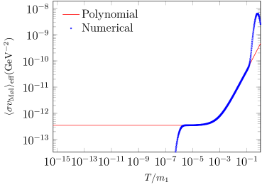
Figure 1: Comparison between the results obtained for $\langle\sigma{v_{\scriptscriptstyle\textrm{M\o l}}}\rangle_{\scriptscriptstyle{\textrm{eff}}}$ by using the full expression (11) and the polynomial expansion at the first order by using (36).

IV Case of particles with small mass splitting

The result shown in section III is correct up to a defined order, under the hypothesis that there are no new physics species with a mass close to the one of the dark matter candidate. In models with a $\mathbb{Z}_{2}$ symmetry, such a particle is the lightest of a set. Let us suppose that there are $M\leq N$ particles nearly degenerate in mass. In such a case, we need to retain their contributions to the denominator in (11). Let us define:

$$x =\frac{m_{1}}{T}, x_{i} =\frac{m_{i}}{T}, c_{i} =\frac{g_{i}}{g_{1}}\frac{m_{i}^{2}}{m_{1}^{2}}, \Delta x_{i} =x_{i}-x,$$ (37)

for $i=1,\dots,M$. We can perform the same change of variable as in section III which leads to:

$$\langle\sigma{v_{\scriptscriptstyle\textrm{M\o l}}}\rangle_{\scriptscriptstyle{\textrm{eff}}} =\frac{x}{2m_{1}^{2}}\frac{1}{\quantity[\sum_{i=1}^{M}c_{i}K_{2}\quantity(\frac{m_{i}}{T})]^{2}}\int_{1}^{+\infty}\differential{y}\sqrt{y-1}W_{\scriptscriptstyle{\textrm{eff}}}(y)K_{1}\quantity(2x\sqrt{y}).$$ (38)

After expanding $W_{\scriptscriptstyle{\textrm{eff}}}$ around $y=1$ as in the previous case we obtain:

$$\langle\sigma{v_{\scriptscriptstyle\textrm{M\o l}}}\rangle_{\scriptscriptstyle{\textrm{eff}}}=\sum\limits_{n=0}^{\infty}\frac{1}{n!}W_{n}\mathcal{H}_{n}(x).$$ (39)

where we have defined:

$$\mathcal{H}_{n}(x) =\frac{x}{2m_{1}^{2}}\frac{1}{\quantity[\sum_{i=1}^{M}c_{i}K_{2}\quantity(\frac{m_{i}}{T})]^{2}}I_{n}(x),$$ (40)

and where $I_{n}$ is the same as the one defined in (19). Note that $\mathcal{H}_{n}$ and $\mathcal{K}_{n}$ differ only for the Bessel functions in the denominator. With some manipulations, we can treat $\mathcal{H}_{n}$ similarly as done with $\mathcal{K}_{n}$. In fact, we already know how to write $I_{n}$ as Laurent series.

Let us define the quantity:

$$D(x) =\quantity[\sum_{i=1}^{M}c_{i}K_{2}\quantity(x_{i})]^{2}.$$ (41)

Our goal is to expand $D(x)$ at its first order in $\Delta x_{i}$ and at an arbitrary order in $x$. Let us expand the square:

$$D(x) =\quantity[\sum_{i=1}^{M}c_{i}K_{2}\quantity(x+\Delta x_{i})]^{2}$$

$$=2\sum_{i=1}^{M}c_{i}K_{2}(x+\Delta x_{i})\sum_{j=i}^{M}\quantity(1-\frac{\delta_{ij}}{2})c_{j}K_{2}(x+\Delta x_{j}).$$ (42)

At the first order in $\Delta x_{i}$ we have also:

$$K_{2}\quantity(x+\Delta x_{i})=K_{2}(x)+K_{2}^{\prime}(x)\Delta x_{i},$$ (43)

where $K_{2}^{\prime}(x)=\derivative{K_{2}}{x}{(x)}$. Therefore:

$$D(x) =2\sum_{i=1}^{M}\sum_{j=i}^{M}c_{i}\quantity(1-\frac{\delta_{ij}}{2})c_{j}\quantity(K_{2}(x)+K_{2}^{\prime}(x)\Delta x_{i})\quantity(K_{2}(x)+K_{2}^{\prime}(x)\Delta x_{j})$$

$$=2\sum_{i=1}^{M}\sum_{j=i}^{M}c_{i}\quantity(1-\frac{\delta_{ij}}{2})c_{j}\quantity(K_{2}^{2}(x)+K_{2}(x)K_{2}^{\prime}(x)\quantity(\Delta x_{i}+\Delta x_{j})+o\quantity(\Delta x^{2})).$$ (44)

Separating the constant terms from the linear terms in $\Delta x_{i}$, and using the identity $2K_{2}(x)K_{2}^{\prime}(x)=K_{2}^{2}(x)$ we obtain:

$$D(x) =\quantity[\sum_{i=1}^{M}\sum_{j=i}^{M}c_{i}\quantity(2-\delta_{ij})c_{j}]K_{2}^{2}(x)+\quantity[\sum_{i=1}^{M}\sum_{j=i}^{M}c_{i}\quantity(1-\frac{\delta_{ij}}{2})c_{j}\quantity(\Delta x_{i}+\Delta x_{j})]\quantity(K_{2}^{2})^{\prime}(x),$$ (45)

where $\quantity(K_{2}^{2})^{\prime}(x)=\derivative{K_{2}^{2}}{x}{(x)}$. Let us define:

$$\tilde{\rho} =\quantity[\sum_{i=1}^{M}\sum_{j=i}^{M}c_{i}\quantity(2-\delta_{ij})c_{j}], \tilde{\eta}=-\quantity[\sum_{i=1}^{M}\sum_{j=i}^{M}c_{i}\quantity(1-\frac{\delta_{ij}}{2})c_{j}\quantity(\Delta x_{i}+\Delta x_{j})],$$ (46)

and use the expansions (65) and (66):

$$D(x) =\frac{\pi}{2x}\mathrm{e}^{-2x}\quantity[\tilde{\rho}(1+B(x))+\tilde{\eta}(2+\tilde{B}(x))]$$

$$=\frac{\pi}{2x}\mathrm{e}^{-2x}\quantity[\tilde{\rho}+2\tilde{\eta}+\tilde{\rho}B(x)+\tilde{\eta}\tilde{B}(x)]$$

$$=\frac{\pi}{2x}\mathrm{e}^{-2x}\gamma\quantity[1+\rho B(x)+\eta\tilde{B}(x)],$$ (47)

with

$$\gamma =\tilde{\rho}+2\tilde{\eta}, \rho =\frac{\tilde{\rho}}{\gamma}, \eta =\frac{\tilde{\eta}}{\gamma}.$$ (48)

We can therefore write:

$$\frac{1}{D(x)}=\frac{2x}{\pi\gamma}\mathrm{e}^{2x}\frac{1}{1+F(x)},$$ (49)

with:

$$F(x)=\rho B(x)+\eta\tilde{B}(x).$$ (50)

The asymptotic behaviour at large $x$ for $F$ is proportional to $1/x$, since for both $B$ and $\tilde{B}$ it is proportional to $1/x$. This means that we can treat (49) with the geometric expansion

$$\frac{1}{D(x)}=\frac{2x}{\pi\gamma}\mathrm{e}^{2x}\sum_{r=0}^{\infty}(-1)^{r}F^{r}(x).$$ (51)

At this point we have found the same form as in the previous case, and we can treat it similarly. Moreover, we have chosen to use the definition (50) for $F$, because it has the advantage of being straightforward to reduce to the order 0 in $\Delta x_{i}$, which is the case if more particles have exactly the same mass. In fact, $\tilde{B}$ is from the first order of the expansion of $K_{2}^{2}(x+\Delta x_{i})$ and also for $\Delta x_{i}=0$ we have $\eta=0$.

Thus, apart from a factor $1/\gamma$ and the replacement $B\to F$, we have found the same expression as in the previous case:

$$\langle\sigma{v_{\scriptscriptstyle\textrm{M\o l}}}\rangle_{\scriptscriptstyle{\textrm{eff}}} =\frac{1}{2\sqrt{\pi}m_{1}^{2}\gamma}{x^{2}}\sum_{r=0}^{\infty}(-1)^{r}F^{r}(x)\sum\limits_{n=0}^{\infty}\quantity[\frac{1}{n!}W_{n}\Gamma\quantity(n+\frac{3}{2})\sum_{p=n+2}^{\infty}g_{n,p}x^{-p}].$$ (52)

This does not change the orders to which we need to truncate the series once we know that we want the result to a given $N_{\scriptscriptstyle{\textrm{max}}}$. By using the results in (29):

$$0\leq r\leq N_{\scriptscriptstyle{\textrm{max}}}, 0\leq n\leq N_{\scriptscriptstyle{\textrm{max}}}, n+2\leq p\leq N_{\scriptscriptstyle{\textrm{max}}}+2.$$ (53)

The difference is that here the coefficients of $F$ up to a given order depend on model-dependent quantities, i.e. $\rho$ and $\eta$. We can use the same procedure as before, since we know that the geometric sum in $F$ has to be truncated at the order $N_{\scriptscriptstyle{\textrm{max}}}$. Hence, it is enough to expand each power $F^{r}$ separately as a function of $B$ and $\tilde{B}$, for which we know the coefficients, at the first order in $\eta$. We automated this calculation in the Wolfram Mathematica notebook in the ancillary files. Parametrising the geometric expansion as:

$$\frac{1}{1+F(x)}= \sum_{r=0}^{\infty}\frac{\phi_{r}}{x^{r}},$$ (54)

we have, for $N_{\scriptscriptstyle{\textrm{max}}}=4$, the following expressions:

$$\phi_{0}= 1,$$ (55a)

$$\phi_{1}= -\eta\tilde{b}_{1}-\rho b_{1},$$ (55b)

$$\phi_{2}= \eta\left(2\rho b_{1}\tilde{b}_{1}-\tilde{b}_{2}\right)+\rho^{2}b_{1}^{2}-\rho b_{2},$$ (55c)

$$\phi_{3}= \eta\left(-3\rho^{2}b_{1}^{2}\tilde{b}_{1}+2\rho b_{1}\tilde{b}_{2}+2\rho b_{2}\tilde{b}_{1}-\tilde{b}_{3}\right)-\rho^{3}b_{1}^{3}+2\rho^{2}b_{2}b_{1}-\rho b_{3},$$ (55d)

$$\phi_{4}= \eta\left(4\rho^{3}b_{1}^{3}\tilde{b}_{1}-3\rho^{2}b_{1}^{2}\tilde{b}_{2}-6\rho^{2}b_{2}b_{1}\tilde{b}_{1}+2\rho b_{1}\tilde{b}_{3}+2\rho b_{3}\tilde{b}_{1}+2\rho b_{2}\tilde{b}_{2}-\tilde{b}_{4}\right)$$

$$+\rho^{4}b_{1}^{4}-3\rho^{3}b_{2}b_{1}^{2}+2\rho^{2}b_{3}b_{1}+\rho^{2}b_{2}^{2}-\rho b_{4}.$$ (55e)

The values of the $b_{i}$’s and $\tilde{b}_{i}$’s can be found in Table 3.

Plugging into the expression of $\langle\sigma{v_{\scriptscriptstyle\textrm{M\o l}}}\rangle_{\scriptscriptstyle{\textrm{eff}}}$, and replacing the $g_{n,p}$ with their values, we obtain:

$$\langle\sigma{v_{\scriptscriptstyle\textrm{M\o l}}}\rangle_{\scriptscriptstyle{\textrm{eff}}}=\frac{1}{{4\gamma m_{1}^{2}}}\Bigg{\{} W_{0}\phi_{0}+\dfrac{1}{x}\Bigg{[}W_{0}\left(\frac{3\phi_{0}}{4}+\phi_{1}\right)+\frac{3W_{1}\phi_{0}}{2}\Bigg{]}$$

$$+\dfrac{1}{x^{2}}\Bigg{[} W_{0}\left(-\frac{3\phi_{0}}{32}+\frac{3\phi_{1}}{4}+\phi_{2}\right)+W_{1}\left(\frac{21\phi_{0}}{8}+\frac{3\phi_{1}}{2}\right)+\frac{15W_{2}\phi_{0}}{8}\Bigg{]}$$

$$+\dfrac{1}{x^{3}}\Bigg{[} W_{0}\phi_{0}\left(\frac{15\phi_{0}}{128}-\frac{3\phi_{1}}{32}+\frac{3\phi_{2}}{4}+\phi_{3}\right)+W_{1}\left(\frac{75\phi_{0}}{64}+\frac{21\phi_{1}}{8}+\frac{3\phi_{2}}{2}\right)$$

$$+W_{2}\left(\frac{195\phi_{0}}{32}+\frac{15\phi_{1}}{8}\right)+\frac{35W_{3}\phi_{0}}{16}\Bigg{]}$$

$$+\dfrac{1}{x^{4}}\Bigg{[} W_{0}\left(\frac{15\phi_{1}}{128}-\frac{3\phi_{2}}{32}+\frac{3\phi_{3}}{4}+\phi_{4}\right)+W_{1}\left(\frac{75\phi_{1}}{64}+\frac{21\phi_{2}}{8}+\frac{3\phi_{3}}{2}\right)$$

$$+W_{2}\left(\frac{195\phi_{1}}{32}+\frac{15\phi_{2}}{8}\right)+\frac{35W_{3}\phi_{1}}{16}+\frac{315W_{4}\phi_{0}}{128}\Bigg{]}\Bigg{\}}.$$ (56)

From this expression one can check that in the previous hypothesis (i.e. $\gamma=\rho=1$ and $\eta=0$) we recover the same coefficients as in (36). This expression, however, is correctly expanded until the order 4 in $1/x$, but it contains some spurious terms of higher orders in $\Delta x_{i}$. In order to eliminate them and consistently truncate at the first order, we have to do some more manipulations. Recalling the definitions (48) and (46):

$$\rho =\frac{1}{1+2\frac{\tilde{\eta}}{\tilde{\rho}}}, \eta =\frac{\tilde{\eta}}{\tilde{\rho}+2\tilde{\eta}},$$ (57)

and now we can identify $\tilde{\eta}$ as the expansion parameter. At the first order we have:

$$\gamma^{-1} =\frac{1}{\tilde{\rho}}\quantity(1-2\frac{\tilde{\eta}}{\tilde{\rho}}), \rho^{n} =1-2n\frac{\tilde{\eta}}{\tilde{\rho}}, \eta =\frac{\tilde{\eta}}{\tilde{\rho}}.$$ (58)

As we knew already, $\eta\sim\Delta x_{i}$, justifying the truncation of higher powers of $\eta$. Since $\tilde{\eta}$ is always divided by $\tilde{\rho}$, we can choose $\eta$ as the expansion parameter.

In the formula (56), we can replace $\gamma$ with $\tilde{\rho}$ and $\phi_{n}$ with:

$$\tilde{\phi}_{n}=\quantity(1-2\eta)\phi_{n}.$$ (59)

We are left with expressing $\tilde{\phi}_{n}$ at the first order in $\eta$:

$$\tilde{\phi}_{0}= 1-2\eta,$$ (60a)

$$\tilde{\phi}_{1}= \eta\left(3b_{1}-\tilde{b}_{1}\right)-b_{1},$$ (60b)

$$\tilde{\phi}_{2}= \eta\left(2b_{1}\tilde{b}_{1}-\tilde{b}_{2}-4b_{1}^{2}+3b_{2}\right)+b_{1}^{2}-b_{2},$$ (60c)

$$\tilde{\phi}_{3}= \eta\left(-3b_{1}^{2}\tilde{b}_{1}+2b_{1}\tilde{b}_{2}+2b_{2}\tilde{b}_{1}-\tilde{b}_{3}+5b_{1}^{3}-8b_{2}b_{1}+3b_{3}\right)-b_{1}^{3}+2b_{2}b_{1}-b_{3},$$ (60d)

$$\tilde{\phi}_{4}= \eta\left(4b_{1}^{3}\tilde{b}_{1}-3b_{1}^{2}\tilde{b}_{2}-6b_{2}b_{1}\tilde{b}_{1}+2b_{1}\tilde{b}_{3}+2b_{3}\tilde{b}_{1}+2b_{2}\tilde{b}_{2}-\tilde{b}_{4}-6b_{1}^{4}\right.$$

$$\left.+15b_{2}b_{1}^{2}-8b_{3}b_{1}-4b_{2}^{2}+3b_{4}\right)+b_{1}^{4}-3b_{2}b_{1}^{2}+2b_{3}b_{1}+b_{2}^{2}-b_{4}.$$ (60e)

The expression for $\langle\sigma{v_{\scriptscriptstyle\textrm{M\o l}}}\rangle_{\scriptscriptstyle{\textrm{eff}}}$ at the first order in $\Delta x_{i}$ and at the 4th order in $x^{-1}$ reads then:

$$\langle\sigma{v_{\scriptscriptstyle\textrm{M\o l}}}\rangle_{\scriptscriptstyle{\textrm{eff}}}=\frac{1}{{4\tilde{\rho}m_{1}^{2}}}\Bigg{\{} W_{0}\tilde{\phi}_{0}+\dfrac{1}{x}\Bigg{[}W_{0}\left(\frac{3\tilde{\phi}_{0}}{4}+\tilde{\phi}_{1}\right)+\frac{3W_{1}\tilde{\phi}_{0}}{2}\Bigg{]}$$

$$+\dfrac{1}{x^{2}}\Bigg{[} W_{0}\left(-\frac{3\tilde{\phi}_{0}}{32}+\frac{3\tilde{\phi}_{1}}{4}+\tilde{\phi}_{2}\right)+W_{1}\left(\frac{21\tilde{\phi}_{0}}{8}+\frac{3\tilde{\phi}_{1}}{2}\right)+\frac{15W_{2}\tilde{\phi}_{0}}{8}\Bigg{]}$$

$$+\dfrac{1}{x^{3}}\Bigg{[} W_{0}\left(\frac{15\tilde{\phi}_{0}}{128}-\frac{3\tilde{\phi}_{1}}{32}+\frac{3\tilde{\phi}_{2}}{4}+\tilde{\phi}_{3}\right)+W_{1}\left(\frac{75\tilde{\phi}_{0}}{64}+\frac{21\tilde{\phi}_{1}}{8}+\frac{3\tilde{\phi}_{2}}{2}\right)$$

$$+W_{2}\left(\frac{195\tilde{\phi}_{0}}{32}+\frac{15\tilde{\phi}_{1}}{8}\right)+\frac{35W_{3}\tilde{\phi}_{0}}{16}\Bigg{]}$$

$$+\dfrac{1}{x^{4}}\Bigg{[} W_{0}\left(\frac{15\tilde{\phi}_{1}}{128}-\frac{3\tilde{\phi}_{2}}{32}+\frac{3\tilde{\phi}_{3}}{4}+\tilde{\phi}_{4}\right)+W_{1}\left(\frac{75\tilde{\phi}_{1}}{64}+\frac{21\tilde{\phi}_{2}}{8}+\frac{3\tilde{\phi}_{3}}{2}\right)$$

$$+W_{2}\left(\frac{195\tilde{\phi}_{1}}{32}+\frac{15\tilde{\phi}_{2}}{8}\right)+\frac{35W_{3}\tilde{\phi}_{1}}{16}+\frac{315W_{4}\tilde{\phi}_{0}}{128}\Bigg{]}\Bigg{\}},$$ (61)

with $\tilde{\rho}$ defined in (46), $\eta$ defined in (58) and $\tilde{\phi}_{n}$s defined in (60). Note that we showed the results at the order 4 since the expression is already very complicated, but the Wolfram Mathematica notebook in the ancillary files allows us to obtain the correct result at any given order. We would like to comment the result, by noticing that, in this form, the coefficients of $x^{-n}$ depend on $T$, but they are linear in $1/T$, therefore, there is a term proportional to $\eta\sim 1/T$ in $\tilde{\phi}_{0}$. However, we recall that the requirement for the mass degeneracy to contribute is to have $\Delta x_{i}$ small enough to allow the expansion (43). At very low temperatures, only the truly degenerate species contribute, and for $\Delta x_{i}=0$ we have $\eta=0$, so the 0th order contribution does not have a divergence, and the only deviation from the previous formula (36) is contained in the $\tilde{\rho}$ in the prefactor. In Figure 2 we show the results for the MSSM, in which we considered the three lightest neutralinos to have the same mass of $200\text{\,}\mathrm{GeV}$.

$n$	$0$	$1$	$2$	$3$	$4$
$\beta_{n}$	$1$	$-\dfrac{15}{4}$	$\dfrac{285}{32}$	$-\dfrac{2115}{128}$	$\dfrac{51435}{2048}$
$\lambda_{n}$	$-2$	$-\dfrac{11}{4}$	$\dfrac{165}{32}$	$-\dfrac{5295}{128}$	$\dfrac{297135}{2048}$

Table 2: Parameters of $\tilde{\phi}_{n}$ in the form $\tilde{\phi}_{n}=\beta_{n}+\eta\lambda_{n}$.

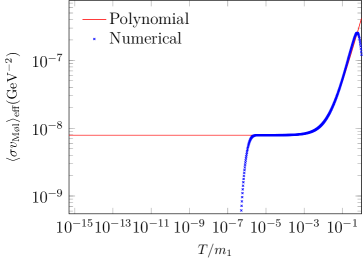
Figure 2: Comparison between the results obtained for $\langle\sigma{v_{\scriptscriptstyle\textrm{M\o l}}}\rangle_{\scriptscriptstyle{\textrm{eff}}}$ using the full expression (11) and the polynomial expansion at the first order by using (61). Plot obtained by using DarkPACK [18].

V Conclusion

We showed in detail how to derive the formula for the expansion of $\langle\sigma{v_{\scriptscriptstyle\textrm{M\o l}}}\rangle_{\scriptscriptstyle{\textrm{eff}}}$ at low temperatures at an arbitrary order in $x=m_{1}/T$ and at the first order in the mass splittings $x_{i}-x$, providing also two Wolfram Mathematica notebooks that allow us to perform both the expansions at an arbitrary order in $x$.

The implementation of formula (36) in the software DarkPACK has shown the necessity of the usage of such an expansion at low temperatures, as the implementation of the full formula (11) fails to provide a numerically stable result. The result is publicly available in DarkPACK 1.2.

As a continuation of this work, we will implement also the formula with mass degeneracy in DarkPACK, allowing to have a more reliable tool for the computation of dark matter densities, especially in models with low freeze-out temperatures.

The overall improved stability of the algorithm in DarkPACK will also be used to solve a system of Boltzmann equations - one for each species at its own temperature $T_{i}$ - to be able to study more general scenarios, in which all the particles of the same species are in thermal equilibrium between them, but not necessarily with the particles of other species. In particular, such hypotheses will allow us the study of freeze-in scenarios, or of models where there is more than one particle as dark matter candidate.

Appendix A Asymptotic expansions of the Bessel functions

The asymptotic form of $K_{n}(z)$ for $\absolutevalue{z}\to+\infty$ and $\absolutevalue{\arg{z}}<3\pi/2$ can be written as [20]:

$$K_{n}(z)\sim\sqrt{\frac{\pi}{2z}}\mathrm{e}^{-z}\quantity[1+\frac{\mu-1}{8z}+\frac{(\mu-1)(\mu-9)}{2!(8z)^{2}}+\frac{(\mu-1)(\mu-9)(\mu-25)}{3!(8z)^{3}}+o\quantity(z^{-4})]$$ (62)

where $\mu=4n^{2}$.

For $n=2$ we define the quantity $A(x)$ such that:

$$K_{2}(x)\sim\sqrt{\frac{\pi}{2x}}\mathrm{e}^{-x}\quantity[1+A(x)]\,,$$ (63)

and we write it in the form:

$$A(x)=\sum_{m=1}^{\infty}a_{m}x^{-m}.$$ (64)

Analogously, we can define the quantity $B(x)$ such that:

$$K_{2}^{2}(x)\sim\frac{\pi}{2x}\mathrm{e}^{-2x}\quantity[1+B(x)]\,,$$ (65)

implying the relation $B=2A+A^{2}$.

Finally, it is helpful to write the asymptotic form of the first derivative of $K_{2}^{2}$ as:

$$\quantity(K_{2}^{2})^{\prime}(x) \sim-\frac{\pi}{2x}\mathrm{e}^{-2x}\quantity[2+\tilde{B}(x)]$$ (66)

with:

$$\tilde{B}(x) =2B(x)+\frac{1}{x}+\frac{B(x)}{x}-B^{\prime}(x)\,.$$ (67)

where the ^′ denotes the derivative with respect to $x$.

$$\begin{array}[]{|c||c|c|c|}\hline\cr m&a_{m}&b_{m}&\tilde{b}_{m}\\ \hline\cr\hline\cr 1&\dfrac{15}{8}&\dfrac{15}{4}&\dfrac{17}{2}\\[8.61108pt] 2&\dfrac{105}{128}&\dfrac{165}{32}&\dfrac{285}{16}\\[8.61108pt] 3&-\dfrac{315}{1024}&\dfrac{315}{128}&\dfrac{1305}{64}\\[8.61108pt] 4&\dfrac{10395}{32768}&\dfrac{315}{2048}&\dfrac{10395}{1024}\\[8.61108pt] 5&-\dfrac{135135}{262144}&-\dfrac{2835}{8192}&\dfrac{315}{4096}\\[8.61108pt] 6&\dfrac{4729725}{4194304}&\dfrac{61425}{65536}&-\dfrac{6615}{32768}\\[8.61108pt] 7&-\dfrac{103378275}{33554432}&-\dfrac{779625}{262144}&\dfrac{80325}{131072}\\[8.61108pt] 8&\dfrac{21606059475}{2147483648}&\dfrac{90904275}{8388608}&-\dfrac{8887725}{4194304}\\[8.61108pt] 9&-\dfrac{655383804075}{17179869184}&-\dfrac{1497971475}{33554432}&\dfrac{138305475}{16777216}\\[8.61108pt] 10&\dfrac{45221482481175}{274877906944}&\dfrac{55124944875}{268435456}&-\dfrac{4793914125}{134217728}\\[8.61108pt] \hline\cr\end{array}$$

Table 3: Coefficients of the Laurent series in the asymptotic expansion of $K_{2}$, $K_{2}^{2}$ and $\quantity(K_{2}^{2})^{\prime}$.

Note that since $A\sim 1/x$, we have $B\sim 1/x$ and $\tilde{B}\sim 1/x$:

$$B(x) =\sum_{m=1}^{\infty}b_{m}x^{-m}, \tilde{B}(x) =\sum_{m=1}^{\infty}\tilde{b}_{m}x^{-m}.$$ (68)

Therefore, the coefficients can be determined using the relations

$$b_{m} =2a_{m}+\sum_{k=1}^{m}a_{k}a_{m-k}, \forall m\geq 1$$ (69)

$$\tilde{b}_{1} =2b_{1}+1, \tilde{b}_{m} =2b_{m}+mb_{m-1}. \forall m\geq 2$$ (70)

The coefficients $a_{m}$ are known, and their values are given in Table 3, thus we can compute all the other parameters.

Appendix B Meijer functions

The Meijer functions are defined as:

$$G^{m,n}_{p,q}\left(z\Bigg{\rvert}\begin{array}[]{c}a_{1},...,a_{n},a_{n+1},...,a_{p}\\ b_{1},...,b_{m},b_{m+1}...,b_{q}\end{array}\right)=\frac{1}{2\pi\mathrm{i}}\int\differential{s}\dfrac{\prod_{j=1}^{m}\Gamma(b_{j}-s)\prod_{j=1}^{n}\Gamma(1-a_{j}+s)}{\prod_{j=m+1}^{q}\Gamma(1-b_{j}+s)\prod_{j=n+1}^{p}\Gamma(a_{j}-s)}x^{s}$$ (71)

where $0\leq m\leq q$, $0\leq n\leq p$, and the poles of $\Gamma(b_{j}-s)$ must not coincide with the poles of $\Gamma(1-a_{j}+s)$ for any pair $(j,k)$ with $1\leq j\leq n$, $1\leq k\leq m$.

The following property holds:

$$\int_{1}^{\infty}\differential xx^{\lambda}(x-1)^{\mu-1}K_{\nu}(a\sqrt{x})=\Gamma(\mu)2^{2\lambda-1}a^{-2\lambda}G_{1,3}^{3,0}\begin{pmatrix}\frac{a^{2}}{4}\Biggr{\rvert}\begin{array}[]{c}0\\ -\mu,\frac{\nu}{2}+\lambda,-\frac{\nu}{2}+\lambda\end{array}\end{pmatrix}.$$ (72)

For $\lambda=0$, $\mu=3/2+n$ and $\nu=1$, the asymptotic form of the $G$-function at the right hand side is:

$$G_{1,3}^{3,0}\begin{pmatrix}x^{2}\Biggr{\rvert}\begin{array}[]{c}0\\ -\frac{1}{2},\frac{1}{2},-n-\frac{3}{2}\end{array}\end{pmatrix}=\sqrt{\pi}\mathrm{e}^{-2x}G_{n}(x),$$ (73)

where $G_{n}(x)$ is a generalized series:

$$G_{n}(x)=\sum_{p=n+2}^{\infty}g_{n,p}x^{-p}.$$ (74)

The results of the expansion of $G_{n}$ for $0\leq n\leq 10$ to the 12th order are:

$$G_{0} =\frac{1}{x^{2}}+\frac{3}{4x^{3}}-\frac{3}{32x^{4}}+\frac{15}{128x^{5}},$$ (75a)

$$G_{1} =\frac{25}{32x^{5}}+\frac{7}{4x^{4}}+\frac{1}{x^{3}},$$ (75b)

$$G_{2} =\frac{13}{4x^{5}}+\frac{1}{x^{4}},$$ (75c)

$$G_{\nu} =\frac{1}{x^{\nu+2}}, \forall\,3\leq\nu\leq 10.$$ (75d)