Parameter-Efficient Transfer Learning of Audio Spectrogram Transformers

Abstract

The common modus operandi of fine-tuning large pre-trained Transformer models entails the adaptation of all their parameters (i.e., full fine-tuning). While achieving striking results on multiple tasks, this approach becomes unfeasible as the model size and the number of downstream tasks increase. In natural language processing and computer vision, parameter-efficient approaches like prompt-tuning and adapters have emerged as solid alternatives by fine-tuning only a small number of extra parameters, without sacrificing performance accuracy. For audio classification tasks, the Audio Spectrogram Transformer model shows impressive results. However, surprisingly, how to efficiently adapt it to several downstream tasks has not been tackled before. In this paper, we bridge this gap and present a detailed investigation of common parameter-efficient methods, revealing that adapters and LoRA consistently outperform the other methods across four benchmarks. Whereas adapters prove to be more efficient in few-shot learning settings, LoRA turns out to scale better as we increase the number of learnable parameters. We finally carry out ablation studies to find the best configuration for adapters and LoRA. Our code is available at: https://github.com/umbertocappellazzo/PETL_AST.

I Introduction

Transfer learning from foundations models pre-trained on a vast amount of data is a well-established paradigm in machine learning, resulting in superb performance across various domains like natural language processing (NLP) [1], vision [2], and speech processing [3, 4]. Typically, when the pre-trained model is adapted to downstream tasks, all its parameters are updated (i.e., full fine-tuning) [5, 6]. Despite its popularity, the full fine-tuning approach suffers some important drawbacks. First of all, given the ever-growing size of pre-trained models, such as GPT-3 [7] (up to $175$ billion parameters) and Whisper Large [8] (1.55 billion parameters), fine-tuning the whole model is often exorbitantly expensive and could potentially result in overfitting, particularly when dealing with a limited-size downstream dataset. Second, this method is storage-inefficient in that it needs to keep a replica of the pre-trained model for every downstream task.

In light of these limitations, some lightweight alternatives, categorized as parameter-efficient transfer learning (PETL), have been introduced for Transformer models [9]. The general idea is to keep most of the pre-trained model’s parameters frozen and instead learn only a small amount of extra parameters. For example, Adapter-tuning introduces small neural modules called adapters to all layers [13]. Typical implementations add the adapter after both the multi-head self-attention (MHSA) and fully connected feed-forward network (FFN) blocks (called Houlsby) [14], or only after the FFN (Pfeiffer) [15]. Another popular approach is LoRA [16], which learns low-rank matrices to approximate parameter updates and reduce the number of trainable parameters. Alternatively, a few task-specific learnable parameters (i.e., prompts) are prepended either to the input sequence (Prompt-tuning) [10, 11], or to the key and value matrices of the MHSA block at each Transformer layer (Prefix-tuning) [12].

While PETL methods have been originally proposed and investigated in NLP and vision domains, more recently they have also been adopted in the speech field. Specifically, prompt-tuning and adapters show competitive performance to full fine-tuning for various speech classification tasks [21, 22] and for Automatic Speech Recognition (ASR) [23, 24, 25]. For audio classification, the Audio Spectrogram Transformer (AST) [19] obtains superb results, standing out as the state-of-the-art model for several downstream tasks. As for the Vision Transformer [18], the problem of how to efficiently transfer the knowledge of the AST is of crucial importance, especially given the typical computational and storage constraints of audio devices. Surprisingly, this topic has received minimal attention. Indeed, only the work in [26] carries out some preliminary experiments on PETL methods for AST, yet its focus is on parameter-efficient continual learning.

Given the above arguments, in this paper, we 1) provide an extensive investigation of the most common PETL approaches applied to the AST model for audio and speech downstream tasks. Our experiments reveal that LoRA and Houlsby adapters achieve the best performance, with LoRA using fewer parameters. To strengthen our analysis, we 2) study their behavior under a few-shot learning setting and 3) how they scale with the number of trainable parameters. We show that adapters perform better in the former scenario, whereas LoRA showcases superior scalability by leveraging an increasing number of parameters. Finally, we 4) present an ablation study for both methods to identify their optimal configuration, underscoring its pivotal role in achieving peak performance.

II Methodology

II-A Recap of the Audio Spectrogram Transformer Architecture

The Audio Spectrogram Transformer is the audio counterpart of the Vision Transformer [18]. It is a convolution-free, purely self-attention-based model that is directly applied to an audio spectrogram, achieving remarkable performance on various audio classification tasks [19, 20]. The input audio undergoes some operations before being fed to the Transformer encoder. First, the input audio waveform of $t$ seconds is converted into a sequence of 128-dimensional log Mel filterbank features, resulting in a $128\times 100\cdot t$ spectrogram. Then, the spectrogram is split into a sequence of $N-1$ $16\times 16$ overlapping patches, which are subsequently flattened through a linear projection layer to a sequence of 1-D patch embeddings, each of size $d=768$. Finally, after prepending the [CLS] token, a trainable positional embedding is added to each patch embedding. The resulting sequence representation $\textbf{X}_{in}\in\mathbb{R}^{N\times d}$ is then used as input to the Transformer encoder.

The Transformer encoder consists of $L$ stacked Transformer layers, each of which is composed of two sub-layers: a multi-head self-attention (MHSA) and a fully-connected feed-forward (FFN) module. The output of the Transformer encoder, $\textbf{X}_{out}\in\mathbb{R}^{N\times d}$, is computed as follows:

$$\mathbf{X}_{out}=\hat{\mathbf{X}}+\text{FFN}(\text{LN}(\hat{\mathbf{X}})),\hat{\mathbf{X}}=\mathbf{X}_{in}+\text{MHSA}(\text{LN}(\mathbf{X}_{in})).$$ (1)

Both blocks, MHSA and FFN, include residual connections and layer normalizations (LN) [27], with the LN applied within the residual branch (i.e., Pre-LN).

The MHSA sub-block allows tokens to share information with one another using self-attention. The conventional attention function maps queries $\mathbf{Q}\in\mathbb{R}^{N\times d_{k}}$ and key-value pairs $\mathbf{K}\in\mathbb{R}^{N\times d_{k}}$, $\mathbf{V}\in\mathbb{R}^{N\times d_{v}}$:

$$Attn(\mathbf{Q},\mathbf{K},\mathbf{V})=softmax(\frac{\mathbf{Q}\mathbf{K}^{T}}{\sqrt{d_{h}}})\mathbf{V}.$$ (2)

Multi-head attention performs the attention function in parallel over $N_{h}$ heads, where each head is separately parameterized by $\mathbf{W}^{(i)}_{q}$, $\mathbf{W}^{(i)}_{k}$, $\mathbf{W}^{(i)}_{v}\in\mathbb{R}^{d\times d_{h}}$ to project inputs to queries, keys, and values, and $d_{k}=d_{v}=d_{h}=d/N_{h}$. The MHSA block computes the output on each head and concatenates:

$$\text{MHSA}= \text{Concat}(\text{head}_{1},\cdots,\text{head}_{N_{h}})\mathbf{W}_{o},$$ (3)

$$\text{head}_{i}=Attn(x\mathbf{W}^{(i)}_{q},x\mathbf{W}^{(i)}_{k},x\mathbf{W}^{(i)}_{v}),$$

with $\mathbf{W}_{o}\in\mathbb{R}^{d\times d}$. In conclusion, the FFN sub-block includes two linear layers with a ReLU activation function in between. If $\textbf{X}_{in}$ is a general input vector, then:

$$\text{FFN}(\textbf{X}_{in})=\text{ReLU}(\textbf{X}_{in}\mathbf{W}_{1}+\textbf{b}_{1})\mathbf{W}_{2}+\textbf{b}_{2},$$ (4)

where $\mathbf{W}_{1}\in\mathbb{R}^{d\times d_{m}}$, $\mathbf{W}_{2}\in\mathbb{R}^{d_{m}\times d}$. In our case, we use $d_{m}=4d$, which is a standard choice for Transformers.

II-B Overview of Parameter-efficient Transfer Learning methods

We now introduce the PETL techniques we used in our experiments: LoRA, prompt/prefix-tuning, and adapter-tuning.

LoRA [16]. LoRA introduces trainable low-rank matrices into Transformer layers to approximate the weight updates. For a pre-trained weight matrix $\mathbf{W}\in\mathbb{R}^{d\times d_{k}}$, LoRA represents its update with a low-rank decomposition $\mathbf{W}+\Delta W=\mathbf{W}+\mathbf{A}\mathbf{B}$, where $\mathbf{A}\in\mathbb{R}^{d\times r}$, $\mathbf{B}\in\mathbb{R}^{r\times d}$ are learnable and $r<<d$. LoRA applies this update to the query and value projection matrices, $\mathbf{W}_{q}$ and $\mathbf{W}_{v}$, in the MHSA sub-layer. LoRA computes the query and value matrices like this:

$$\mathbf{Q}/\mathbf{V}=\mathbf{X}_{in}\mathbf{W}_{q/v}+s\cdot\mathbf{X}_{in}\mathbf{A}_{q/v}\mathbf{B}_{q/v},$$ (5)

where $s\geq 1$ is a tunable scalar hyperparameter.

Prefix-tuning/Prompt-tuning [12, 10]. Prefix-tuning [12] inserts $p$ learnable continuous embeddings of dimension $d$ (i.e., prompts) to the keys and values of the MHSA block at every layer. Prompt-tuning, instead, prepends the prompts in the input space after the projection layer. Following [11], we consider the “shallow” prompt-tuning version (SPT) where all the prompts are prepended to the first Transformer layer, and the “deep” version (DPT) by prepending the prompts uniformly to each Transformer layer.

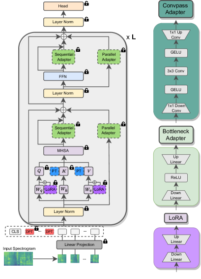
Figure 1: Illustration of the AST model and the PETL methods. Note that adapters are inserted either parallel or sequentially. On the right we schematize the structure of Bottleneck and Convpass adapters, as well as LoRA module.

Adapters [14, 15]. The adapter-tuning approach incorporates small modules (adapters) within the Transformer layers. In its simplest form, the adapter layer is typically composed of a down-projection matrix $\mathbf{W}_{down}\in\mathbb{R}^{d\times r}$ to project the input vector to a lower-dimensional space specified by the bottleneck dimension $r$, followed by a non-linear activation function $f(\cdot)$, and an up-projection matrix $\mathbf{W}_{up}\in\mathbb{R}^{d\times r}$. This design choice is usually referred to as Bottleneck [13, 14].

Adapter-tuning is a flexible approach in that we can identify multiple ways in which an adapter can be included in a Transformer layer, resulting in different configurations. 1) The adapter module can be inserted only after the FNN block, denoted as Pfeiffer [15], or after both the MHSA and FNN blocks, known as Houlsby [14]. 2) The adapter module can be included sequentially, either after the FFN block [14] (i.e., sequential Bottleneck) or after both FFN and MHSA blocks [28] (i.e., sequential Houlsby), or parallel to only the FFN block [29, 30], or parallel to both FFN and MHSA blocks [17]. 3) In computer vision, another popular adapter design is Convpass [17], which consists of three convolutional layers: a $1\times 1$ down-projection convolutional layer, a $3\times 3$ convolution intermediate layer, and a $1\times 1$ up-projection layer. Convpass adapter explicitly introduces inductive bias due to the convolution layers tailored for computer vision tasks. Figure 1 depicts all the described PETL methods.

Mathematically, if we consider the configuration in which the Bottleneck adapter is placed sequentially after the FFN sub-block as an example, and we let $\mathbf{X}_{\text{FFN}}=\text{FFN}(\text{LN}(\hat{\textbf{X}}))$ following the notation in Eq. 2, then the output is:

$$\mathbf{X}_{out}=\hat{\mathbf{X}}+f(\mathbf{X}_{\text{FFN}}\mathbf{W_{down}})\mathbf{W_{up}}.$$ (6)

For the parallel case, we have:

$$\mathbf{X}_{out}=\hat{\mathbf{X}}+\mathbf{X}_{\text{FFN}}+f(\hat{\mathbf{X}}\mathbf{W_{down}})\mathbf{W_{up}}.$$ (7)

III Experiment and Discussion

III-A Experiment Settings

Datasets. We evaluate the PETL methods on three audio/speech downstream tasks. (1) Audio classification: we use the ESC-50 and UrbanSound8K (US8K) datasets. ESC-50 [31] consists of $2000$ 5-second-long environmental audio recordings spanning $50$ classes. US8K [32] includes $8732$ labeled sound excerpts of urban sounds from $10$ classes. (2) Keyword spotting: Speech Commands V2 [33] has $105,829$ 1-second recordings of $35$ common speech commands. (3) Intent classification: Fluent Speech Commands (FSC) [34] includes $30043$ English utterances spanning $31$ intent classes.

PETL methods. We include two traditional fine-tuning strategies: full fine-tuning (Full-FT), which finetunes the entire pre-trained AST model and the classification head; and linear probing, which keeps the backbone frozen and only fine-tunes the head. We then study various PETL methods: shallow prompt-tuning (SPT), deep prompt-tuning (DPT), prefix-tuning (Pref-T), and BitFit [35], which is a common baseline that fine-tunes only the bias terms of the pre-trained backbone. We finally include LoRA and adapters, and we categorize the latter based on 1) which design module is used (Bottleneck or Convpass), 2) whether the Pfeiffer (PF) or Houlsby (HOU) configuration is used, and 3) how the adapter is inserted into each Transformer layer, either in parallel (par) or sequentially (seq). By default, the PF adapter module is placed in the MHSA layer, which we will show is the best configuration (see Table III).

TABLE I: Full results of various PETL methods over 4 datasets. The best and second-best methods for each dataset are highlighted in bold and underlined, respectively.

Method	# params	ESC-50	US8K	GSC	FSC	Avg
Full FT	85.5M	87.48	84.31	97.31	93.29	90.07
Linear	9-40K	75.85	77.93	41.78	27.52	55.77
BitFit	102K	86.05	82.17	85.51	63.85	79.40
SPT-300	230K	84.30	79.73	75.28	40.85	70.04
DPT-25	230K	86.52	83.67	89.18	68.60	81.99
Pref-T 24	221K	82.93	81.39	83.46	55.75	75.88
Bottleneck Adapter
PF par	249K	88.38	83.44	91.33	73.19	84.09
PF seq	249K	86.77	82.86	91.41	72.45	83.37
HOU par	498K	88.00	82.80	91.75	78.71	85.32
HOU seq	498K	87.75	83.28	91.76	76.45	84.81
Convpass Adapter
PF par	254K	87.85	82.72	92.27	72.84	83.92
PF seq	254K	86.15	83.10	89.21	70.31	82.19
HOU par	508K	87.15	82.75	92.55	77.79	85.06
HOU seq	508K	87.58	83.06	89.45	74.02	83.53
LoRA	221K	86.45	83.83	93.61	76.00	84.97

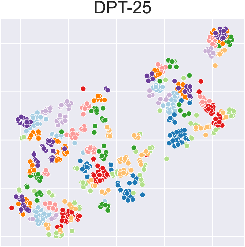
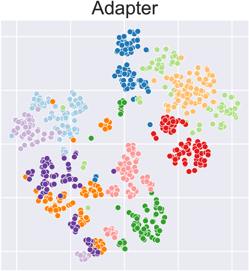
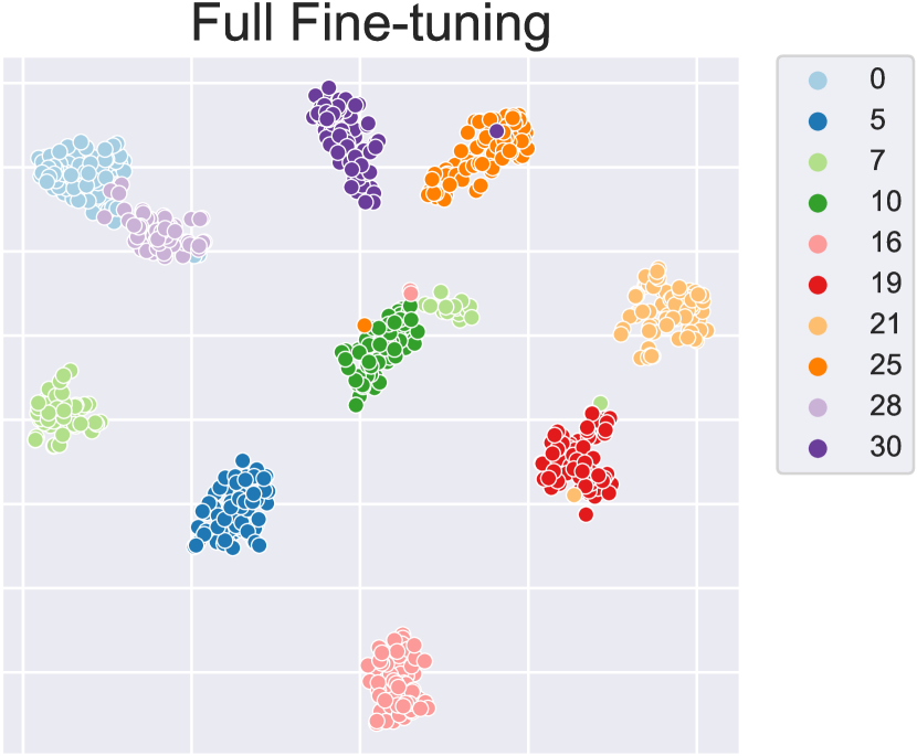
Figure 2: t-SNE plots for the FSC dataset using the projection of the [CLS] token. We include 10 classes for clarity.

Setup details. For all experiments we use the AST model pre-trained on ImageNet-21K [37] and AudioSet [38] provided by the Huggingface Transformers library [39]. The hidden dimension is $d=768$. For the final classification, we use a simple linear layer (head), which uses the entire output sequence for the final classification (i.e., [CLS] + audio embeddings). For all datasets, we use AdamW optimizer with cosine annealing scheduler and weight decay set to $0.1$. The initial learning rate is $0.005$ for adapters and LoRA methods, while for the three prompt-tuning methods is $0.01$. As reported in [36], we also observed that the latter are rather sensitive to hyperparameters. The dimension of the intermediate space for adapters and LoRA is computed as $r=d/\text{RR}$, where RR is the reduction rate. Unless otherwise stated, RR is set to $64$ and $128$ for adapters and LoRA, respectively. For LoRA, following [16], the scaling factor is $s=\alpha/\text{RR}$, where $\alpha$ = 8 leads to the best results. As a final remark, for a fair comparison, we choose the number of prompts and the reduction rate RR to ensure that the methods use approximately the same amount of parameters. The total number of parameters lies in the range [$230,500$]K, which corresponds to $0.3$-$0.6\%$ of the Full FT approach. For a complete overview of the hyperparameters, please refer to our github repository.

III-B Main Results and Discussion

Main Results. In Table I, we report the results for the PETL methods across the four datasets. First of all, we see that Houlsby adapters and LoRA achieve the best results on average. Pfeiffer adapters perform slightly worse, yet they still surpass the other PETL methods (DPT, Pref-T, BitFit). We also notice two interesting findings for adapters: a) the parallel adapter turns out to be more competitive than sequential, and b) the Convpass adapter, despite the use of convolutional layers, performs on par or even worse than Bottleneck.

Overall, the results obtained by the PETL methods are close to or surpass the Full FT method for the audio tasks, while for GSC and even more for FSC, the results are worse. We posit that this happens because the AST model is pre-trained on Audioset [38] which only partially includes speech clips. This is confirmed also by the fact that the linear baseline achieves good performance for the audio datasets, while for the speech ones, the results are poor, showing that training a linear head on top of the frozen feature embeddings is not sufficient. Finally, Figure 2 shows t-SNE [40] visualization of the [CLS] token after the last layer for the FSC dataset. We see that adapters produce reasonable linearly separable representations (similar results are obtained for LoRA, which we do not include for lack of space), not as neat as Full FT but using far fewer parameters. DPT-25, instead, struggles to disentangle the underlying manifold structure of the task.

To bolster the previous results, in Figure 3 we study the trend of the methods as a function of the number of trainable parameters (to increase/decrease the parameters, we decrease/increase RR accordingly). We see that LoRA exhibits superior scalability than adapters and DPT for both datasets.

Few-shot setting. We also test the PETL methods under a few-shot setting. Table II reveals that adapters attain the best results when few labeled samples are available, making them the best option for few-shot learning.

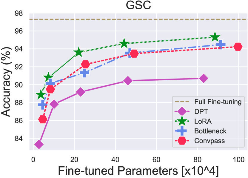
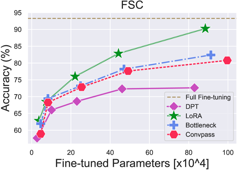
Figure 3: Results of various PETL methods in function of the number of learnable parameters for the GSC and FSC datasets.

TABLE II: Few-shot learning analysis for ESC-50/GSC. We use parallel insertion for PF Bottleneck/Convpass adapters.

	ESC-50				GSC
	Examples per class
Method	1	2	4	8	2	8	32	64
DPT-25	32.7	44.3	57.0	71.9	9.4	18.7	43.1	57.1
LoRA	31.8	42.2	58.8	70.7	6.8	15.2	41.8	59.8
Bottle	33.0	45.5	60.2	72.8	7.2	16.0	47.9	66.6
Conv	32.6	45.4	60.3	73.2	7.3	16.2	47.8	66.8

III-C Ablation Studies on Adapters and LoRA

We now investigate 1) where and how to insert the adapter module into the AST model, and 2) which matrices in the MHSA layer are to be approximated by LoRA in order to achieve the best results.

TABLE III: Ablation study on the optimal config. of adapters.

Configuration	ESC-50	US8K	GSC	FSC	Avg
FFN-Seq/Par-After	86.77	82.86	91.41	72.45	83.37
FFN-Seq-Before	54.68	71.60	86.80	61.44	68.63
FFN-Par-Before	87.07	82.72	90.84	72.08	83.18
MHSA-Seq/Par-After	87.80	83.08	89.30	64.40	81.15
MHSA-Seq-Before	76.03	81.30	90.74	73.76	80.46
MHSA-Par-Before	88.38	83.44	91.33	73.19	84.09

TABLE IV: Ablation study on the optimal config. of LoRA.

Config.	$\mathbf{W}_{q}$	$\mathbf{W}_{q},\mathbf{W}_{k}$	$\mathbf{W}_{q},\mathbf{W}_{v}$	$\mathbf{W}_{q},\mathbf{W}_{k},\mathbf{W}_{v},\mathbf{W}_{o}$
RR	64	128	128	256
ESC-50	83.05	84.15	86.45	86.15
US8K	82.56	82.35	83.83	83.51
GSC	89.08	91.51	93.61	94.08
FSC	61.84	65.59	76.00	78.90
Avg	79.13	80.90	84.97	85.66

Where and how to insert the adapter. There are multiple ways in which an adapter can be inserted into a Transformer layer, such as parallel to the FFN block [29], or sequentially to the FFN block [30]. However, since none of these configurations prevails over the others, but rather seems to depend on the considered downstream task and dataset, we try to figure out the optimal way to place the adapter. We try $6$ configurations, based on where and how we put the adapter: 1) into the FFN or MHSA sub-layer, 2) after or before the selected sub-layer, and 3) parallel (Par) or sequentially (Seq). In Table III we report the results for Bottleneck adapters and we see that the MHSA-Par-Before configuration obtains the best results, but also Seq/Par-After and Par-Before for FFN achieve good results, showing that, despite some small differences, adapters are flexible in terms of their insertion location.

Best configuration for LoRA. Finally, we study which MHSA weight matrices should LoRA approximate in order to achieve the best results. Based on [16], we select $4$ configurations and we choose the RR such that the number of parameters remains constant across them (i.e., 221K) for fair comparison. In Table IV we can observe that approximating with LoRA all the weight matrices of the MHSA sub-layer results in the best configuration. The adaptation of ($\textbf{W}_{q}$,$\textbf{W}_{v}$) achieves slightly worse results, yet it is the best configuration for the audio datasets. On the contrary, the other two configurations get inferior accuracy. Our results confirm previous results for LLMs [16].

IV Conclusion and Future Work

In this work, we study the problem of parameter-efficient transfer learning for the AST model. Exhaustive experiments spanning four audio and speech datasets reveal that LoRA and adapters obtain the best results overall. If adapters perform better under a few-shot learning scenario, LoRA is the best option when more parameters can be allocated. We also conduct ablation studies on the optimal configuration for adapters and LoRA. We finally notice that there still exists a gap between Full FT and adapters/LoRA for speech tasks, thus suggesting that more investigation is necessary. In this direction, future work will explore new adapter modules tailored for speech.

We include in the appendix some additional experiments we conducted. Specifically, we investigate: 1) what is the best adapter configuration given a fixed budget of parameters, 2) whether combining multiple PETL methods brings about further improvement, and 3) the role of residual connections in the learning process. We finally provide some additional results on the ESC-50 dataset.

-A How to Optimally Allocate a Given Budget for Adapters

TABLE V: Ablation study on the optimal adapter configuration given a specific number of trainable params.

Method	# params	ESC-50	FSC	Avg
PF FFN-Seq-After	249K	86.77	72.45	79.61
PF MHSA-Par-Before	249K	88.38	73.19	80.79
PF FFN-Seq-After x2	470K	87.18	73.60	80.39
PF MHSA-Par-Before x2	470K	88.50	78.19	83.35
HOU seq	498K	87.75	76.45	82.10
HOU par	498K	88.00	78.71	83.35
HOU mixed	498K	87.75	78.41	83.08
HYDRA FFN [41]	470K	87.25	76.18	81.72

We assume we have a certain amount of parameters to allocate for an adapter module. In principle, the Houlsby configuration, due to its design, exploits twice as many parameters as the Pfeiffer configuration because it introduces two adapters, one for the MHSA sub-layer and one for the FFN. For this reason, we provide a fairer comparison between the Houlsby and Pfeiffer configurations by constraining the former to have two adapters whose size is half that used by the Pfeiffer configuration (we achieve this by halving the reduction rate RR to $32$). We include the best configurations that we found from the analysis in Table III: FFN-Seq-After and MHSA-Par-Before. We add the word “x2” to emphasize that the adapter’s size is double that of the individual adapters used by Houlsby.

For the Houlsby configuration, we report three variants: 1) HOU seq, which adds both the adapters sequentially after the MHSA/FFN sub-layers; 2) HOU par, which adds parallel adapters before the MHSA/FFN sub-layers; 3) HOU seq adds one parallel adapter before the MHSA sub-layer and one adapter sequentially after the FFN sub-layer, reflecting the finding that the MHSA and FFN sub-layers have different best configurations. Finally, we also include a recent configuration called HYDRA [41], which proposes to leverage both parallel and sequential adapters. We report the results for the case in which the adapters are included in the FFN sub-layer like in the original paper. While we tried to do the same for the MHSA layer, we found that this configuration led to poor and unstable results, thus we do not include it.

The results are reported in Table V. We can observe that the best configurations for Pfeiffer (PF FFN-Par-Before x2) and Houlsby (HOU par) achieve the same results, thus showing that having one adapter or two adapters with half size leads to very similar results. Furthermore, the table suggests that it seems better to have one adapter for each sub-layer when the downstream task is more challenging (FSC). As a final comment, we observe that the concurrent use of parallel and sequential adapters (i.e., HYDRA) performs worse than the previous methods.

-B On the Combination of Multiple PETL Methods

In this section, we try to combine adapters with DPT/LoRA. This study stems from a recent work called NOAH (Neural Prompt Search) [42], which combines these three methods and performs neural architecture search on the reduction rate of adapter and LoRA, as well as on the number of prompts $p$ used by DPT. In our case, we choose RR and $p$ such that the combinations of approaches use roughly the same number of parameters, thus they are not learned by the model itself. Since DPT and LoRA work on the MHSA sub-layer, we decide to apply the adapter module parallel to the FFN layer. For the setting in which we use all three methods, the RR of LoRA is set to $256$ and that of the adapter is kept to $64$.

From Table VI, we see that combining adapters and LoRA does not bring additional improvements. TWith respect to LoRA alone, adding a parallel adapter is beneficial to ESC-50 because we see that adapters alone perform better than LoRA, but for FSC adding adapters to LoRA deteriorates the performance. Instead, the use of DPT seems to deteriorate the performance for both datasets, and so it does when all the three methods are used concurrently. All in all, we can conclude that, depending on the dataset at hand, the use of a single PETL methods is the best choice.

TABLE VI: Ablation study on the combination of multiple PETL methods.

Method	# params	ESC-50	FSC	Avg
PF MHSA-Par-Before x2	470K	88.50	78.19	83.35
HOU par	498K	88.00	78.71	83.35
LoRA	442k	86.70	82.84	84.77
Adapter + LoRA	470K	88.00	81.54	84.77
Adapter + DPT-25	479K	86.60	77.15	81.88
Adapter + DPT-14 + LoRA	488K	86.80	79.83	83.32

TABLE VII: Ablation study on the use of residual connections for sequential/parallel Bottleneck adapters.

Residual	Seq/Par	ESC-50	FSC
✓	Seq	86.77	72.45
✗	Seq	69.20	56.48
✗	Par	87.07	72.08
✓	Par	73.20	69.28

-C On Residual Connections

We here ablate the use of residual connections for adapters. We focus on Bottleneck, RR $=64$, FFN case. Table VII shows that residuals are necessary for sequential adapters, while they must be avoided for parallel adapters. Indeed, for the sequential case, the residual connection allows the model to have direct access to the FFN output, whereas the parallel adapter can be seen already as a residual.

-D Additional Experiments on ESC-50

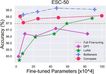
Figure 4: PETL methods performance on the ESC-50 dataset when more and more parameters are available.

We finally include Figure 4 where we show how the PETL methods scale with respect to the number of parameters for the ESC-50 dataset, which we do not include in the main paper for space constraints. We see that LoRA manages to approach adapters only when the budget of parameters is close to $1$ million, whereas adapters need a small number of parameters to achieve strong results, and adding more and more parameters does not lead to better performance (for Bottleneck adapter using more parameters is even deleterious). This behavior is in line with what we show in the main paper, namely that LoRA is able to scale better as more parameters are available, whilst it struggles when dealing with few parameters or labeled data. The main difference of LoRA and MHSA adapters is that LoRA approximates the query and value projection matrices, whereas adapters try to approximate the entire MHSA sub-layer function.

References

- [1] J. Devlin, M. Chang, K. Lee, and K. Toutanova, “Bert: Pre-training of deep bidirectional transformers for language understanding,” in Proceedings of NAACL, 2019.
- [2] A. Kolesnikov et al., “Big Transfer (BiT): General Visual Representation Learning,” in European conference on computer vision (ECCV), Springer, 2020, pp. 491–507.
- [3] Y. Wang, A. Boumadane, and A. Heba, “A fine-tuned wav2vec 2.0/Hubert benchmark for speech emotion recognition, speaker verification and spoken language understanding,” 2021, arXiv preprint arXiv:2111.02735.
- [4] U. Cappellazzo, E. Fini, M. Yang, D. Falavigna, A. Brutti, and B. Raj, “Continual Contrastive Spoken Language Understanding,” 2023, arXiv preprint arXiv:2310.02699.
- [5] E. Tsalera, A. Papadakis, and M. Samarakou, “Comparison of pre-trained CNNs for audio classification using transfer learning,” J. Sensor Actuator Netw., vol. 10, no. 4, p. 72, Dec. 2021.
- [6] C. Raffel et al., “Exploring the limits of transfer learning with a unified text-to-text transformer,” The Journal of Machine Learning Research, 2020, 21.1: 5485-5551.
- [7] T. Brown et al., “Language models are few-shot learners,” in Advances in neural information processing systems, 2020, vol. 33, pp. 1877-1901.
- [8] A. Radford et al., “Robust speech recognition via large-scale weak supervision,” in International Conference on Machine Learning, 2023, pp. 28492-28518.
- [9] N. Ding et al., “Delta tuning: A comprehensive study of parameter efficient methods for pre-trained language models,” 2022, arXiv preprint arXiv:2203.06904.
- [10] B. Lester, R. Al-Rfou, and N. Constant, “The power of scale for parameter-efficient prompt tuning,” in Proceedings of EMNLP, 2021.
- [11] J. Menglin et al., “Visual prompt tuning,” in European Conference on Computer Vision. Cham: Springer Nature Switzerland, 2022. pp. 709-727.
- [12] X. L. Li, and P. Liang, “Prefix-tuning: Optimizing continuous prompts for generation,” in Proceedings of ACL, 2021.
- [13] S. Rebuffi, H. Bilen, and A. Vedaldi, “Learning multiple visual domains with residual adapters,” in Advances in neural information processing systems, 30, 2017.
- [14] N. Houlsby et al., “Parameter-efficient transfer learning for NLP,” in International Conference on Machine Learning, PMLR, 2019, pp. 2790-2799.
- [15] J. Pfeiffer et al., “Adapter-Fusion: Non-destructive task composition for transfer learning,” in Proceedings of EACL, 2021.
- [16] E. Hu et al., “LoRA: Low-rank adaptation of large language models,” 2021, arXiv preprint arXiv:2106.09685.
- [17] S. jie, and Z. Deng, “Convolutional bypasses are better vision transformer adapters,” arXiv preprint arXiv:2207.07039, 2022.
- [18] A. Dosovitskiy et al., “An image is worth 16×16 words: Transformers for image recognition at scale,” in Proceedings of the 9th International Conference on Learning Representations, 2021.
- [19] Y. Gong, Y.-A. Chung, and J. Glass, “AST: Audio spectrogram transformer,” in Proc. Interspeech, 2021, pp. 571–575.
- [20] Y. Gong, C.I. Lai, Y.-A. Chung, and J. Glass, “Ssast: Self-supervised audio spectrogram transformer,” in Proceedings of the AAAI Conference on Artificial Intelligence, 2022, vol. 36, pp. 10699-10709.
- [21] K. Chang et al., “Speechprompt v2: Prompt tuning for speech classification tasks,” 2023, arXiv preprint arXiv:2303.00733.
- [22] Z. Chen et al., “Exploring efficient-tuning methods in self-supervised speech models,” in IEEE Spoken Language Technology Workshop (SLT), 2022, pp. 1120-1127.
- [23] B. Thomas, S. Kessler, and S. Karout, “Efficient adapter transfer of self-supervised speech models for automatic speech recognition,” in ICASSP, 2022, pp. 7102-7106.
- [24] S. Kessler, B. Thomas, and S. Karout, “An adapter based pre-training for efficient and scalable self-supervised speech representation learning,” in ICASSP, 2022, pp. 3179-3183.
- [25] S. Otake, R. Kawakami, and N. Inoue, “Parameter Efficient Transfer Learning for Various Speech Processing Tasks,” in ICASSP, 2023, pp. 1-5.
- [26] NM Selvaraj et al., “Adapter Incremental Continual Learning of Efficient Audio Spectrogram Transformers,” 2023, arXiv preprint arXiv:2302.14314.
- [27] J. L. Ba, J. R. Kiros, and G. E Hinton, “Layer normalization,” 2016, arXiv preprint arXiv:1607.06450.
- [28] R. K. Mahabadi, S. Ruder, M. Dehghani, and J. Henderson, “Parameter-efficient multi-task fine-tuning for transformers via shared hypernetworks,” in Annual Meeting of the Association for Computational Linguistics, 2021.
- [29] J. He, C. Zhou, X. Ma, T. Berg-Kirkpatrick, and G. Neubig, “Towards a Unified View of Parameter-Efficient Transfer Learning,” in International Conference on Learning Representations, 2022.
- [30] S. Chen et al., “Adaptformer: Adapting vision transformers for scalable visual recognition,” in Advances in Neural Information Processing Systems, 2022, vol. 35, pp. 16664-16678.
- [31] K. J. Piczak, “ESC: Dataset for environmental sound classification,” in Proceedings of the 23rd ACM international conference on Multimedia, 2015, pp. 1015-1018.
- [32] J. Salamon, C. Jacoby, and J. P. Bello, “A dataset and taxonomy for urban sound research,” in Proceedings of the 22nd ACM international conference on Multimedia, 2014, pp. 1041-1044.
- [33] P. Warden, “Speech commands: A dataset for limited-vocabulary speech recognition,” 2018, arXiv preprint arXiv:1804.03209.
- [34] L. Lugosch, M. Ravanelli, P. Ignoto, V. S. Tomar, and Y. Bengio, “Speech model pre-training for end-to-end spoken language understanding,” 2019, arXiv preprint arXiv:1904.03670.
- [35] E. Ben Zaken, Y. Goldberg, and S. Ravfogel, “BitFit: Simple Parameter-efficient Fine-tuning for Transformer-based Masked Language-models,” in Proceedings of the 60th Annual Meeting of the Association for Computational Linguistics, 2022, vol. 2, pp. 1-9.
- [36] T. Vu et al., “SPoT: Better Frozen Model Adaptation through Soft Prompt Transfer,” in Proceedings of the 60th Annual Meeting of the Association for Computational Linguistics, 2022, vol.1 , pp. 5039-5059.
- [37] J. Deng, W. Dong, R. Socher, L.-J. Li, K. Li, and L. Fei-Fei, “ImageNet: A large-scale hierarchical image database,” in CVPR, 2009.
- [38] J. F. Gemmeke et al., “Audio Set: An ontology and human-labeled dataset for audio events,” in ICASSP, 2017.
- [39] T. Wolf et al., “Huggingface’s transformers: State-of-the-art natural language processing,” 2019, arXiv preprint arXiv:1910.03771.
- [40] L. Van Der Maaten, and G. Hinton, “Visualizing data using t-SNE,” Journal of machine learning research, 2008, 9.11.
- [41] S. Kim et al., “Hydra: Multi-head Low-rank Adaptation for Parameter Efficient Fine-tuning,” 2023, arXiv preprint arXiv:2309.06922.
- [42] Y. Zhang, K. Zhou, and Z. Liu, “Neural Prompt Search,” 2022, arXiv preprint arXiv:2206.04673.