Efficient Learning in Polyhedral Games via Best Response Oracles

Abstract

We study online learning and equilibrium computation in games with polyhedral decision sets, a property shared by normal-form games (NFGs) and extensive-form games (EFGs), when the learning agent is restricted to utilizing a best-response oracle. We show how to achieve constant regret in zero-sum games and $O(T^{1/4})$ regret in general-sum games while using only $O(\mathop{{\rm log}}t)$ best-response queries at a given iteration $t$, thus improving over the best prior result, which required $O(T)$ queries per iteration. Moreover, our framework yields the first last-iterate convergence guarantees for self-play with best-response oracles in zero-sum games. This convergence occurs at a linear rate, though with a condition-number dependence. We go on to show a $O(1/\sqrt{T})$ best-iterate convergence rate without such a dependence. Our results build on linear-rate convergence results for variants of the Frank-Wolfe () algorithm for strongly convex and smooth minimization problems over polyhedral domains. These results depend on a condition number of the polytope, known as facial distance. In order to enable application to settings such as EFGs, we show two broad new results: 1) the facial distance for polytopes of the form $\{{\bm{x}}\in{\mathbb{R}}^{n}_{\geq 0}\mid{\mathbf{A}}{\bm{x}}={\bm{b}}\}$ is at least $\gamma/\sqrt{k}$ where $\gamma$ is the minimum value of a nonzero coordinate of a vertex in the polytope and $k\leq n$ is the number of tight inequality constraints in the optimal face, and 2) the facial distance for polytopes of the form ${\mathbf{A}}{\bm{x}}={\bm{b}},{\mathbf{C}}{\bm{x}}\leq{\bm{d}},{\bm{x}}\geq\mathbf{0}$ where ${\bm{x}}\in{\mathbb{R}}^{n}$, ${\mathbf{C}}\geq\mathbf{0}$ is a nonzero integral matrix, and ${\bm{d}}\geq\bm{0}$, is at least $1/(\|{\mathbf{C}}\|_{\infty}\sqrt{n})$. This yields the first such results for several problems, such as sequence-form polytopes, flow polytopes, and matching polytopes.

1 Introduction

Learning in games is a well-studied framework in which agents iteratively refine their strategies through repeated interactions with their environment. One natural way for agents to iteratively refine their strategies is by best-responding. This idea can be applied in many forms, the simplest and earliest instance of which was fictitious play () (Brown, 1951). This algorithm involves the agent observing the strategies played by the opponent and then playing a strategy that corresponds to the best response to the average of the observed strategies. This algorithm was shown to converge (Robinson, 1951), but its convergence rate can, in the worst case, scale quite poorly with the number of actions available to each player (Daskalakis and Pan, 2014). It is then natural to ask what are the best convergence guarantees that can be obtained for the computation of Nash equilibria in two-player zero-sum games or coarse correlated equilibria in multiplayer games when agents are learning through a best-response oracle.

In the online learning community, methods based only on best-response oracles are special cases of methods based on a linear minimization oracle (LMO), which can be queried for points that minimize a linear objective over the feasible set. Such methods are known as projection-free methods because they avoid potentially expensive projections onto the feasible set. Projection-free online learning algorithms might perform multiple LMO calls per iteration, so our paper and related literature are concerned not only with the number of iterations $T$ of online learning but also the total number of LMO calls, which we will denote by $N$. Because LMOs for polyhedral decision sets essentially correspond to a best-response oracle (BRO), we will use these two terms interchangeably.

Follow the Perturbed Leader () (Kalai and Vempala, 2005) was the first such algorithm. When used by both players in two-player zero-sum games, it yields a $O(1/\sqrt{T})$ convergence rate to Nash equilibrium, with a single LMO call in each iteration. More recently, Suggala and Netrapalli (2020) propose an optimistic variant of (); achieves a $O(1/T)$ rate of convergence to Nash equilibrium but requires $O(T)$ LMO calls per iteration, thus corresponding to a $O(1/\sqrt{N})$ rate as a function of the total number of LMO calls. Online Frank-Wolfe (OFW) (Hazan and Kale, 2012) is another projection-free algorithm, based on the well-studied Frank-Wolfe () algorithm (Frank and Wolfe, 1956). While it does not require multiple calls to an LMO, it can only achieve a $O(T^{-1/3})$ rate for two-player zero-sum games. We aim to break the $O(1/\sqrt{N})$ barrier in terms of convergence towards two-player zero-sum equilibria and beyond. We focus on the setting of polyhedral games, a class containing both normal-form and extensive-form games. Our primary contribution is an online learning method which enjoys $O(1/T)$ average individual regret in zero-sum games and $O(1/T^{3/4})$ average individual regret in general-sum games while only requiring $O(\mathop{{\rm log}}t)$ LMO calls in iteration $t$. Table 1 compares our algorithm with other algorithms with the best-known guarantees for the setting we consider. In the table, we also include a non-optimistic version of our algorithm; despite having worse theoretical guarantees than existing projection-free algorithms, it outperforms them in our numerical experiments.

Independent of work in projection-free online learning, there has also been substantial work developing BRO-based algorithms in the game-solving community. Most prominent is the Double Oracle (DO) algorithm (McMahan et al., 2003) for computing Nash equilibria in two-player zero-sum games, which uses BROs and a meta-solver for computing Nash equilibria in a restricted game formed by the returned iterates. More recently, the Policy Space Response Oracle framework (Lanctot et al., 2017), a generalization of Double Oracle, has laid the foundation for the design of DO-variants. These algorithms only have theoretical guarantees for computing Nash equilibria in two-player zero-sum games, require a meta-solver for solving the restricted game composed of the strategies chosen by the players at each iteration, and thus are centralized, and do not have convergence rate guarantees to equilibria.

The optimization community has also done substantial work on developing projection-free methods, spurred by the work of Frank and Wolfe (1956). Guarantees for typically assume the function $f$ being optimized is smooth (has Lipschitz gradient) and convex, the domain ${\cal X}$ being optimized over is convex and compact, and that the algorithm has access to a first-order oracle for the function which returns gradients $\nabla f({\bm{x}})$ at a queried point ${\bm{x}}$ and an LMO which returns solutions to minimization problems of the form $\mathop{\rm argmin}_{{\bm{x}}\in{\cal X}}\langle{\bm{c}},{\bm{x}}\rangle$ for any choice of ${\bm{c}}\in{\mathbb{R}}^{n}$. Given an initial iterate ${\bm{x}}^{(0)}$, it produces new iterates given by the following update rule:

$${\bm{x}}^{(t+1)} =\frac{t}{t+2}{\bm{x}}^{(t)}+\frac{2}{t+2}\mathop{\rm argmin}_{{\bm{x}}^{\prime}\in{\cal X}}\langle\nabla f({\bm{x}}^{(t)}),{\bm{x}}^{\prime}\rangle.$$

In recent years, there has been work on developing -based approaches to saddle-point computation (e.g., Gidel et al. (2017); Lan and Zhou (2016)). However,  Gidel et al. (2017) only has fast convergence guarantees for strongly convex-concave objectives and Lan and Zhou (2016) are only able to provide $O(1/\sqrt{N})$ convergence to saddle-points. On the other hand, our method is able to leverage a variant, away-step Frank-Wolfe (), to achieve faster convergence rates.

1.1 Contributions

We present a projection-free online learning method, Approximate Reflected Online Mirror Descent, using away-step Frank-Wolfe (), for learning over compact and convex polyhedral decision sets. uses reflected online mirror descent (), an optimistic online learning algorithm which requires a prediction of the next loss, instantiated with the Euclidean regularizer. The proximal problem for this setup is thus strongly convex and smooth. Using the linear convergence of for polyhedral domains, we implement approximate steps of using only a logarithmic number of iterations. We show that even with approximate steps, still yields an approximate regret bounded by variation in utilities (RVU) bound (Syrgkanis et al., 2015), a form of regret guarantee that depends on how much the observed utilities vary, and which has enabled proving constant regret of optimistic learning dynamics in two-player zero-sum games and $O(T^{1/4})$ regret in general games (Syrgkanis et al., 2015). While using -based methods to approximate proximal steps has been previously studied, pioneered by work of  Lan and Zhou (2016), it is a surprising blind spot in the literature that the connection to regret guarantees for games has not previously been made.

We then apply our algorithm to learning in games using only BROs (as opposed to typical learning algorithms, which require access to Euclidean projection or other proximal oracles). We show that when every player employs , it is possible to converge to a Nash equilibrium in a two-player zero-sum game at a rate of $O(\mathop{{\rm log}}N/N)$, where $N$ is the number of BRO calls. In contrast, the best prior results converged at a rate of $O(1/\sqrt{N})$ (Suggala and Netrapalli, 2020). More generally, we show that requires only $O(\mathop{{\rm log}}t)$ best-response queries at each self-play iteration $t$ while guaranteeing constant social regret, as well as $O(T^{1/4})$ regret for each player after $T$ total iterations of self-play. We go on to study the last-iterate convergence properties of in self-play in zero-sum settings. We show that, indeed it is possible to retain last-iterate convergence under , and in fact, it converges at a linear rate (up to error induced by the approximate proximal computation). To the best of our knowledge, these are both the first last-iterate convergence and the first linear-rate convergence results for self-play dynamics that purely rely on best-response oracles. As with existing linear-rate results in the literature (Tseng, 1995; Gilpin et al., 2012; Wei et al., 2021), we have a dependence on a condition number inherent to the game, which is generally hard to evaluate. We show that if one wishes to avoid this condition-number dependence, then self-play with still achieves a $O(1/\sqrt{T})$ best-iterate convergence. Our convergence results to Nash equilibria and coarse correlated equilibria are summarized below using the following two informal theorems:

Theorem 1 (Informal; Full version in Theorems 6, 8 and 9).

Using a $\epsilon^{\prime}$-Nash equilibrium in a two-player zero-sum game can be computed in $O(1/\epsilon^{\prime})$ iterations and $O(\frac{1}{\epsilon^{\prime}}\mathop{{\rm log}}{\frac{1}{\epsilon^{\prime}}})$ LMO calls. Furthermore, in two-player zero-sum games, will produce an iterate which is a $\epsilon^{\prime}$-Nash equilibrium in $O(\frac{1}{\epsilon^{\prime 2}}\mathop{{\rm log}}{\frac{1}{\epsilon^{\prime}}})$ iterations without a dependence on a problem-dependent constant. will produce an iterate which is a $\epsilon^{\prime}$-Nash equilibrium in $O(\mathop{{\rm log}}{\frac{1}{\epsilon^{\prime}}})$ iterations, with this convergence rate having a dependence on a game-dependent constant. Exact dependence on problem parameters can be found in the formal theorems.

Theorem 2 (Informal; Full version in Theorem 7).

In multiplayer games, can be used to compute a $\epsilon^{\prime}$-coarse correlated equilibrium in $O(\frac{1}{\epsilon^{\prime\frac{4}{3}}}\mathop{{\rm log}}\frac{1}{\epsilon^{\prime}})$ iterations. Exact dependence on problem parameters can be found in the formal theorem.

The linear convergence of on polyhedral domains is crucial to our result, but the particular rate depends on the facial distance constant of the polytope in question (in addition to the strong convexity and smoothness constants). To that end, we show two novel lower bounds on the facial distance of a polytope. Our first result concerns polytopes that can be described in the form ${\mathbf{A}}{\bm{x}}={\bm{b}},{\bm{x}}\geq\mathbf{0}$ where ${\bm{x}}\in\mathbb{R}^{n}$. Let $\gamma$ be the minimum value of a nonzero coordinate of a vertex in the polytope. Then, we show that the facial distance is at least $\gamma/\sqrt{n}$.

Moreover, if the optimal solution lies in a face such that $k\leq n$ inequality constraints $x_{i}\geq 0$ are tight, then the rate dependence in can be tightened to $\frac{\gamma}{\sqrt{k}}$. This theorem immediately implies several useful results, including a bound $1/\sqrt{n}$ on the facial distance of the sequence-form polytope, which is the polytope describing the set of feasible strategies of a player in an EFG, where $n$ is the number of sequences for the player. It also implies similar results for flow polytopes and matching polytopes. The fact that the facial distance is only square-root power small in the dimension of the problem ensures that the convergence rate of linearly convergent variants over these polytopes does not scale poorly as the ambient dimension of the problem increases. Our second result concerns an integral polytope ${\cal X}$ given by ${\mathbf{A}}{\bm{x}}={\bm{b}},{\mathbf{C}}{\bm{x}}\leq{\bm{d}},{\bm{x}}\geq\mathbf{0}$ where ${\bm{x}}\in{\mathbb{R}}^{n}$, where ${\mathbf{C}}\geq\bm{0}$ is a nonzero integral matrix, and ${\bm{d}}\geq\bm{0}$. In particular, for integral polytopes, we are able to handle inequality constraints. In that case, we show that the facial distance is at least $1/(\|{\mathbf{C}}\|_{\infty}\sqrt{n})$.

Finally, we conduct experiments to demonstrate that our algorithm performs well in practice relative to other projection-free algorithms when computing Nash and coarse correlated equilibria in polyhedral games.

	$\nabla$ computations	LMO calls	Social regret	Avg. social regret
Algorithm	at iteration $t$	at iteration $t$	$\sum_{i}{\mathrm{Reg}}_{i}^{(T)}$	$\sum_{i}\frac{1}{T}{\mathrm{Reg}}_{i}^{(T)}$
(Kalai and Vempala, 2005)	$O(1)$	$O(1)$	$O(\sqrt{T})$	$O(1/\sqrt{N})$
Optimistic () (Suggala and Netrapalli, 2020)	$O(1)$	$O(T)$	$O(1)$	$O(1/\sqrt{N})$
[this paper]	$O(1)$	$O(\mathop{{\rm log}}t)$	$O(\sqrt{T})$	$O(\sqrt{\mathop{{\rm log}}N/N})$
[this paper]	$O(1)$	$O(\mathop{{\rm log}}t)$	$O(1)$	$O(\mathop{{\rm log}}N/N)$

Table 1: A comparison of the number of gradient ($\nabla$) computations, number of LMO calls, cumulative regret (as a function of the total number of iterations $T$), and average regret (as a function of total LMO calls $N$) of various projection-free algorithms. In two-player zero-sum games, average social regret upper bounds the duality gap to Nash equilibrium for the averaged iterates.

1.2 Related Work

Frank-Wolfe algorithm.

Frank and Wolfe (1956) presented the original Frank-Wolfe () algorithm (also known as conditional gradient descent), a projection-free first-order method for solving smooth constrained convex minimization problems. Vanilla provides a $O(\frac{1}{t})$ rate of convergence for smooth objectives, but has stronger guarantees for special classes of functions; in particular, for strongly convex functions, Garber and Hazan (2015) showed a $O(\frac{1}{t^{2}})$ convergence rate. Many variants have been developed since Frank and Wolfe’s original presentation of the algorithm, including the away-step variant (Wolfe, 1970). Importantly for us, Lacoste-Julien and Jaggi (2015) showed that and several other variants achieve linear convergence for strongly convex and smooth objectives over polyhedral domains; see also Pena and Rodriguez (2019); Beck and Shtern (2017). There are several excellent overviews of Frank-Wolfe algorithms, e.g., Jaggi (2013); Bomze et al. (2021); Braun et al. (2022).

for saddle-point problems.

There has been some work on extending to saddle-point problems, prominently by  Gidel et al. (2017). However, they only provide fast convergence guarantees for strongly convex-concave objectives (and moreover, require a significant degree of strong convexity, thus rendering their results incompatible with smoothing techniques). They do provide a convergence guarantee for the bilinear case when the feasible sets are polytopes, but it is extremely slow. Lan (2016) introduced the idea of “gradient sliding,” which involves computing approximate prox steps to save on the number of gradient computations required to optimize a composite function with a smooth and nonsmooth component. In the spirit of this work, Lan and Zhou (2016) introduced “conditional gradient sliding,” which involves using conditional gradient methods to compute these approximate prox steps. They combine this idea with Nesterov acceleration to achieve $O(1/\sqrt{\epsilon})$ gradient computations and $O(1/\epsilon)$ LMO calls for smooth functions. They present a smoothed version of their algorithm as well that can be applied to saddle-point problems, but the smoothing degrades the guarantee to $O(1/\epsilon)$ gradient computations and $O(1/\epsilon^{2})$ LMO calls.

Projection-free online learning.

The first projection-free online learning algorithm was , introduced by Kalai and Vempala (2005). The algorithm involves randomly perturbing the sum of the observed losses (which serves as a form of regularization, see e.g., Abernethy et al. (2016)) before computing the best response, and achieves $O(1/\sqrt{T})$ average regret for linear loss functions.  Suggala and Netrapalli (2020) introduced , which achieves $O(1/T)$ average regret for players in zero-sum games but requires doing $O(T)$ LMO calls at every iteration.  Hazan and Kale (2012) presented OFW which uses to achieve $O(1/T^{1/4})$ average regret for Lipschitz convex losses.

Algorithms for game solving.

There has been much work done to develop efficient algorithms for game-solving. We only touch on the major trends related to discrete-time methods and sequential games. A line of research has focused on constructing no-regret algorithms with ergodic convergence to equilibrium. Out of these, we highlight two categories: methods based on the CFR regret-decomposition framework (Zinkevich et al., 2007; Farina et al., 2021b; Tammelin et al., 2015; Brown and Sandholm, 2019a; Lanctot et al., 2009), and methods based on the OMD framework and more generally first-order methods (Hoda et al., 2010; Kroer et al., 2020; Farina et al., 2021a, 2022b). Some of these methods were key in solving large games, such as poker (Bowling et al., 2015; Brown and Sandholm, 2018, 2019b). A recent trend has focused on establishing learning algorithms with (poly)logarithmic per-player regret when used in self-play, including Anagnostides et al. (2023, 2022b); Daskalakis et al. (2015, 2021); Wibisono et al. (2022); Anagnostides et al. (2022a); Farina et al. (2022a). These methods are able to compute equilibria in multiplayer games at the rate of $\tilde{O}(1/T)$. Finally, another recent trend in the literature has focused on establishing learning algorithms (Wei et al., 2021; Lee et al., 2021) and first-order methods (Tseng, 1995; Gilpin et al., 2012) with guarantees for last-iterate convergence.

2 Notation and Preliminaries

We will use $\|\cdot\|_{p}$ to denote the ${\bm{\ell}}_{p}$-norm and $\|\cdot\|$ without subscript to denote $\|\cdot\|_{2}$. Any norm-dependent quantity (e.g., diameter, facial distance, strong convexity, and smoothness) will be with respect to the Euclidean norm (which is self-dual) unless otherwise noted. Because we are principally concerned with using these algorithms for equilibrium computation in games, we will use subscripts to indicate a set or constant corresponding to a particular agent. We will use $[n]$ to denote the set $\{1,\dots,n\}$, and $L$-smoothness refers to Lipschitz continuity of the gradient, with modulus $L$.

2.1 Online Linear Optimization

In online learning, an agent $i$ repeatedly interacts with an environment, aiming to minimize its regret. At each time $t$, the agent chooses a strategy ${\bm{x}}_{i}^{(t)}$ from a given feasible set ${\cal X}_{i}\subseteq{\mathbb{R}}^{n_{i}}$ and then receives a loss vector ${\bm{\ell}}^{(t)}_{i}\in{\cal X}_{i}\to{\mathbb{R}}$. The loss is allowed to depend adversarially on ${\bm{x}}_{i}^{(t)}$. The agent then pays a cost of $\langle{\bm{\ell}}_{i}^{(t)},{\bm{x}}_{i}^{(t)}\rangle$. The (cumulative) regret ${\mathrm{Reg}}_{i}^{(T)}$ after $T$ iterations is defined as $\max_{{\bm{x}}^{\prime}\in{\cal X}_{i}}\sum_{t=1}^{T}\langle{\bm{\ell}}_{i}^{(t)},{\bm{x}}_{i}^{(t)}\rangle-\langle{\bm{\ell}}_{i}^{(t)},{\bm{x}}^{\prime}\rangle$, and average regret is defined as regret divided by the number of iterations. We will assume that losses are bounded and normalized: $\|{\bm{\ell}}^{(t)}_{i}\|\leq 1$ for all $t\in[T]$.

In order to achieve desired regret guarantees, online learning algorithms typically require some form of regularization. While achieves this regularization through randomization, the framework of algorithms utilizing approximate prox calls that we present will require access to a regularizer ${\varphi}_{i}:{\cal X}_{i}\to{\mathbb{R}}$, which is 1-strongly convex and $L_{i}$ smooth on ${\cal X}_{i}$. The Bregman divergence between ${\bm{x}},{\bm{y}}\in{\cal X}_{i}$ is denoted by $\divi{{\bm{x}}}{{\bm{y}}}$. Furthermore, we define $\Omega_{i}\mathrel{:\mkern-0.25mu=}\sup_{{\bm{x}},{\bm{y}}\in{\cal X}_{i}}\divi{{\bm{x}}}{{\bm{y}}}$ and $D_{i}\mathrel{:\mkern-0.25mu=}\sup_{{\bm{x}},{\bm{y}}\in{\cal X}_{i}}\|{\bm{x}}-{\bm{y}}\|$. $\delta({\cal X}_{i})$ will be used for the facial distance of ${\cal X}_{i}$, defined in Section 2.4. For a given set, ${\cal X}$, and a point ${\bm{x}}\in{\cal X}$, we denote $\mathop{{\rm dist}}({\bm{x}},{\cal X})\mathrel{:\mkern-0.25mu=}\inf_{{\bm{x}}^{\prime}\in{\cal X}}\|{\bm{x}}-{\bm{x}}^{\prime}\|$ and in the case that ${\cal X}$ is compact, define $\Pi_{{\cal X}}({\bm{x}})=\mathop{\rm argmin}_{{\bm{x}}^{\prime}\in{\cal X}}\lVert{\bm{x}}-{\bm{x}}^{\prime}\rVert$.

Online Mirror Descent (OMD) is an algorithm which performs a single proximal computation at every iteration of the algorithm, generating iterates as follows:

$${\bm{x}}_{i}^{(t+1)}=\mathop{\rm argmin}_{{\bm{x}}_{i}\in{\cal X}_{i}}\biggl{\{}\langle{\bm{\ell}}_{i}^{(t)},{\bm{x}}_{i}\rangle+\frac{1}{\eta}\divi{{\bm{x}}_{i}}{{\bm{x}}_{i}^{(t)}}\biggr{\}}.$$

It enjoys $O(1/\sqrt{T})$ average regret (e.g.,  Hazan et al. (2016); Orabona (2019)).

Reflected Online Mirror Descent () is an optimistic version of OMD which utilizes a prediction ${\bm{m}}_{i}^{(t+1)}$ of the next loss ${\bm{\ell}}_{i}^{(t+1)}$ to generate the iterate at time $t+1$.

$${\bm{x}}_{i}^{(t+1)} =\mathop{\rm argmin}_{{\bm{x}}_{i}\in{\cal X}_{i}}\biggl{\{}\langle{\bm{\ell}}_{i}^{(t)}+{\bm{m}}_{i}^{(t+1)}-{\bm{m}}_{i}^{(t)},{\bm{x}}_{i}\rangle+\frac{1}{\eta}\divi{{\bm{x}}_{i}}{{\bm{x}}_{i}^{(t)}}\biggr{\}}.$$

It is common to use the last observed loss as the prediction for the next loss: set ${\bm{m}}_{i}^{(t+1)}$ equal to ${\bm{\ell}}_{i}^{(t)}$. In this case, achieves $O(1/T)$ average regret (Malitsky, 2015; Joulani et al., 2017) in self-play. Since ${\bm{m}}_{i}^{(t+1)}$ is the prediction of a loss ${\bm{\ell}}_{i}^{(t+1)}$ which is assumed to have norm bounded by 1, we will assume that $\|{\bm{m}}_{i}^{(t)}\|\leq 1$ for all $t\in[T]$.

Syrgkanis et al. (2015) introduce the notion of Regret bounded by Variation in Utilities (RVU), recalled next, and demonstrate that algorithms with this property exhibit faster convergence to equilibria in games.

Definition 1 (RVU (Syrgkanis et al., 2015)).

A learning algorithm for Player $i$ is said to satisfy the RVU property if for some $\alpha,\beta,\gamma>0$, and all possible ${\bm{\ell}}_{i}^{(1)},\dots,{\bm{\ell}}_{i}^{(T)}$,

$${\mathrm{Reg}}_{i}^{(T)}\leq\alpha+\beta\sum_{t=1}^{T}\|{\bm{\ell}}_{i}^{(t)}-{\bm{\ell}}_{i}^{(t-1)}\|^{2}-\gamma\sum_{t=1}^{T}\|{\bm{x}}_{i}^{(t)}-{\bm{x}}_{i}^{(t-1)}\|^{2}.$$

satisfies this inequality with $\alpha=\Omega/\eta$, $\beta=\eta$, $\gamma=1/4\eta$; we are not aware of a reference for this, but it can be shown very similarly to known results for optimistic OMD. Later we will show in Lemma 2 that our approximate in Algorithm 1 still satisfies the RVU property.

2.2 Game-Theoretic Notions

Normal-form games (NFGs) model single-shot simultaneous interactions among a set of agents denoted by $[N]$. The agents each have a set of possible actions ${\cal A}_{i}$ and a normalized utility function $u_{i}:\prod_{i\in[N]}{\cal A}_{i}\rightarrow[-1,1]$, the latter specifying their payoff for a given choice of actions by each of the agents. The game is said to be zero-sum if $\sum_{i\in[n]}u_{i}({\bm{a}})=0$ for all ${\bm{a}}\in\prod_{i\in[N]}{\cal A}_{i}$. A mixed-strategy ${\bm{x}}_{i}$ for Player $i$, is a probability distribution over ${\cal A}_{i}$; ${\bm{x}}_{i}\in\Delta({\cal A}_{i})$. We can extend the domain of $u_{i}$ to be over $\Delta({\cal A}_{i})$ by taking the expectation of the utility function over the distribution over ${\cal A}_{i}$ induced by ${\bm{x}}_{i}\in\Delta({\cal A}_{i})$.

Nash equilibrium is the de facto notion of equilibrium in NFGs, and the problem of computing a Nash equilibrium (NE) in two-player zero-sum games can be formulated as a bilinear saddle-point problem (BSPP):

$$\min_{{\bm{x}}\in{\cal X}}\max_{{\bm{y}}\in{\cal Y}}\langle{\mathbf{A}}{\bm{x}},{\bm{y}}\rangle.$$ (BSPP)

In this case, ${\cal X}$ and ${\cal Y}$ are the space of mixed strategies for Player 1 and Player 2, respectively, and ${\mathbf{A}}$ encodes the utility of Player 2 for a given choice of strategies for both players. The duality gap $\xi$ of $\bar{{\bm{x}}}$ and $\bar{{\bm{y}}}$ for (BSPP) can be defined as $\max_{{\bm{y}}\in{\cal Y}}\langle{\mathbf{A}}\bar{{\bm{x}}},{\bm{y}}\rangle-\min_{{\bm{x}}\in{\cal X}}\langle{\mathbf{A}}{\bm{x}},\bar{{\bm{y}}}\rangle$. This quantity is typically used to measure the quality of a solution; in the case of two-player zero-sum games, a duality gap of $\epsilon^{\prime}$ corresponds to an $\epsilon^{\prime}$-NE (and thus is also known as Nash gap).

Definition 2 ($\epsilon^{\prime}$-coarse correlated equilibrium).

An $\epsilon^{\prime}$-coarse correlated equilibrium ($\epsilon^{\prime}$-CCE) is defined as ${\bm{x}}\in\Delta(\prod_{i\in[N]}{\cal A}_{i})$ such that

$$\mathbb{E}_{{\bm{a}}\sim{\bm{x}}}[u_{i}({\bm{a}})]\geq\mathbb{E}_{{\bm{a}}_{-i}\sim{\bm{x}}}[u_{i}({\bm{a}}^{\prime}_{i},{\bm{a}}_{-i})]-\epsilon^{\prime}$$

for all players $i\in[N]$, for all ${\bm{a}}^{\prime}_{i}\in{\cal A}_{i}$, for $\epsilon^{\prime}\geq 0$; $\epsilon^{\prime}=0$ corresponds to an exact CCE.

Extensive-form games (EFGs) are a generalization of normal-form games, which also allow for modeling of sequential moves (and also private and/or imperfect information and stochasticity). Equilibrium computation for two-player zero-sum EFGs can also be formulated as (BSPP), by letting ${\cal X}$ and ${\cal Y}$ be convex polytopes known as sequence-form polytopes (Romanovskii, 1962; Koller et al., 1996; von Stengel, 1996), and letting ${\mathbf{A}}$ be a matrix representing the utility of Player 2 for a given choice of strategies for both players. An important property that sequence-form polytopes have is they can be expressed in the form ${\mathbf{A}}{\bm{x}}={\bm{b}},{\bm{x}}\geq 0$; this will allow us to characterize the facial distance of these polytopes. Additional background on EFGs can be found in Appendix B.

When we are analyzing multiplayer games involving $N$ agents, we will let ${\cal X}_{i}\subset{\mathbb{R}}^{n_{i}}$ denote the convex and compact set of strategies for the $i^{th}$ player, where $i\in[N]$, and let ${\bm{x}}_{i}\in{\cal X}_{i}$ represent their strategy. For NFGs, ${\cal X}_{i}$ is $\Delta({\cal A}_{i})$, the set of mixed strategies for $i$, while for EFGs, ${\cal X}_{i}$ is the sequence-form polytope for Player $i$. In the case of two-player zero-sum NFGs or EFGs, in which case Nash equilibrium computation corresponds to (BSPP), we will let ${\cal X}={\cal X}_{1}$, ${\cal Y}={\cal X}_{2}$, and $\mathcal{Z}={\cal X}\times{\cal Y}$. In this case, we will use $\mathcal{Z}^{*}$ to denote the set of solutions to the BSPP. We define the vector field $\bm{F}({\bm{z}})=({\mathbf{A}}^{T}{\bm{y}},-{\mathbf{A}}{\bm{x}})$ for ${\bm{z}}\in\mathcal{Z}$. Without loss of generality, we assume that $\bm{F}$ is smooth with constant 1 (the payoff matrix ${\mathbf{A}}$ can be scaled to ensure this is the case).

2.3 Saddle-Point Metric-Subregularity

Problems of the form (BSPP) satisfy a condition known as Saddle-Point Metric Subregularity (Wei et al., 2021) as long as ${\cal X}$ and ${\cal Y}$ are convex polytopes (this is the case for NFGs and EFGs).

Definition 3 (Saddle-Point Metric Subregularity).

The SP-MS condition is satisfied if for any ${\bm{z}}\in\mathcal{Z}\setminus\mathcal{Z}^{*}$ with ${\bm{z}}^{*}=\Pi_{\mathcal{Z}}({\bm{z}})$ for some $\beta\geq 0$ and $\nu>0$,

$$\sup_{{\bm{z}}^{\prime}\in\mathcal{Z}}\frac{\langle\bm{F}({\bm{z}}),{\bm{z}}-{\bm{z}}^{\prime}\rangle}{\|{\bm{z}}-{\bm{z}}^{\prime}\|}\geq\nu\|{\bm{z}}-{\bm{z}}^{*}\|^{\beta+1}.$$ (SP-MS)

For any given NFG or EFG, there exists $\nu\geq 0$ so that Equation SP-MS holds with $\beta=0$; given a choice of a game, we will use $\nu$ to refer to this problem-dependent constant. Wei et al. (2021) use this condition to demonstrate linear last-iterate convergence of certain online learning algorithms. Earlier works (Tseng, 1995; Gilpin et al., 2012) showed linear last-iterate convergence using error bounds, and Wei et al. (2021) note that there is a close correspondence between the SP-MS condition and error bound techniques for bilinear polyhedral settings.

2.4 Frank-Wolfe and Facial Distance

Frank-Wolfe is a projection-free algorithm that converges with rate $O(1/T)$ for smooth convex functions over convex compact sets. In certain situations, faster convergence rates can be obtained; for example, when the function is strongly convex and the optimal solution lies in the relative interior of the feasible set, the original algorithm is linearly convergent (Guélat and Marcotte, 1986). In the case where the optimal solution is not in the interior, away-step Frank Wolfe () is a variant of Frank-Wolfe which was shown to achieve linear convergence for strongly convex objectives over polyhedral sets (Wolfe, 1970; Guélat and Marcotte, 1986; Lacoste-Julien and Jaggi, 2015). Pseudocode for is provided in Appendix A. The linear rate of and several other linearly convergent variants of depends on a condition number of the polytope known as the facial distance. It can be defined concisely using a theorem from (Pena and Rodriguez, 2019):

Definition 4 (Facial distance, Pena and Rodriguez (2019)).

$$\delta({\cal P})=\min_{\begin{subarray}{c}{\cal F}\in\operatorname{faces}({\cal P})\\ \emptyset\subseteq{\cal F}\subseteq{\cal P}\end{subarray}}\mathop{{\rm dist}}({\cal F},\mathop{{\rm Conv}}(\operatorname{Vert}({\cal P})\setminus{\cal F})).$$

For linearly convergent methods for strongly convex functions, the ratio between the strong convexity modulus and smoothness constant appears as a term in the linear rate. For linearly convergent variants, both the former ratio and the ratio between the facial distance and diameter over the polyhedral domain appear as terms in the linear rate.

Theorem 3 (Convergence rate of for strongly convex functions over polyhedral sets (Lacoste-Julien and Jaggi, 2015)).

In order to compute an $\epsilon$-optimal solution to a 1-strongly convex, $L$-smooth function over a convex polytope that has diameter $D$ and facial distance $\delta$, requires $O(\frac{LD^{2}}{\delta^{2}}\mathop{{\rm log}}\frac{LD}{\epsilon})$ LMO calls.

This dependence on the facial distance to diameter ratio makes it desirable to have a lower bound on the facial distance, to ensure that the linear rate scales well with the size of the problem.

3 New Results on Polyhedral Facial Distance

In this section, we present two theorems which characterize lower bounds on the facial distance in special cases where the constraints of the polytope can be written in a certain form. The proofs are deferred to Appendix C.

Theorem 4.

Let ${\cal P}$ be a polytope given by ${\mathbf{A}}{\bm{x}}={\bm{b}},{\bm{x}}\geq\mathbf{0}$ where ${\bm{x}}\in\mathbb{R}^{n}$. Let $\gamma$ be the minimum value of a nonzero coordinate of a vertex. Then $\delta({\cal P})\geq\frac{\gamma}{\sqrt{n}}$. Moreover, if the optimal solution lies in a face ${\cal F}$ such that $k$ coordinates are zero (i.e., $|\{i:x_{i}=0\}|=k$), then $\delta({\cal P})\geq\frac{\gamma}{\sqrt{k}}$.

Corollary 1.

For any $0/1$-polytope ${\cal X}$, $\delta({\cal X})\geq\frac{1}{\sqrt{n}}$.

The corollary follows by noting that Theorem 4 holds with $\gamma=1$ for $0/1$ polytopes. Note that simplices (the strategy spaces of NFGs), sequence-form polytopes (the strategy spaces of EFGs), flow polytopes, and matching polytopes are all $0/1$ polytopes. The fact that the facial distance decreases only at a square-root rate in the dimension of the problem ensures reasonable scaling of as the ambient dimension of the problem increases.

In the case we are dealing with integral polytopes (polytopes with integral vertices), we can also handle inequality constraints beyond the non-negativity constraints.

Theorem 5.

Let ${\cal P}$ be an integral polytope given by ${\mathbf{A}}{\bm{x}}={\bm{b}},{\mathbf{C}}{\bm{x}}\leq{\bm{d}},{\bm{x}}\geq\mathbf{0}$ where ${\bm{x}}\in{\mathbb{R}}^{n}$, with ${\mathbf{C}}\geq\bm{0}$ a nonzero integral matrix, and ${\bm{d}}\geq\bm{0}$. Then $\delta({\cal P})\geq\frac{1}{\|{\mathbf{C}}\|_{\infty}\sqrt{n}}$.

We note that facial distance and essentially equivalent notions, have been considered non-trivial to evaluate (Garber and Meshi, 2016; Bashiri and Zhang, 2017; Braun et al., 2022) for most polytopes besides hypercubes, unit $\ell_{1}$ balls and simplices. Thus, our lower bounds contribute to a more complete characterization of convergence rates of linearly convergent variants over a fairly broad class of polytopes.

4 Approximate Reflected Online Mirror Descent using Away-step Frank-Wolfe

In this section, we propose an algorithmic framework that uses approximate proximal updates instead of exact proximal updates. First, we will show that such an approximate variant of still retains many of the nice properties of , up to the error in the approximation oracle. Then, we propose the use of linearly convergent variants of for implementing the approximate proximal step, specifically when the regularizer is smooth, and strongly convex (as is the case with the Euclidean regularizer) and the decision set is a convex polytope, which is the case in NFGs and EFGs. We abstract away the concept of computing an approximate proximal update using what we call an approximate proximal oracle (APO).

Definition 5 (Approximate proximal oracle).

An _X, given a choice of convex and compact set ${\cal X}$, takes as input a function $f:{\cal X}\to{\mathbb{R}}$, a $L$-smooth and 1-strongly convex regularizer ${\varphi}$, a prox center ${\bm{x}}_{c}$, and a desired accuracy $\epsilon\geq 0$, and returns ${\bm{x}}^{\prime}\in{\cal X}$ such that

$$f({\bm{x}}^{\prime})+\div{{\bm{x}}^{\prime}}{{\bm{x}}_{c}}\leq\min_{{\bm{x}}\in{\cal X}}\Big{\{}f({\bm{x}})+\div{{\bm{x}}}{{\bm{x}}_{c}}\Big{\}}+\epsilon.$$ (APO)

While our framework can be adapted to a variety of online learning algorithms, we illustrate the framework using in Algorithm 1. ${\bm{x}}_{i}^{(t)}$ is the iterate returned by the algorithm at iteration $t$, ${\bm{\ell}}_{i}^{(t)}$ is the loss received at iteration $t$, and ${\bm{m}}_{i}^{(t)}$ is the prediction of the loss to be used at iteration $t$. Proofs for results in this section are deferred to Appendix D. The subscript $i$ is dropped in statements about a single regret-minimizing agent applying the algorithm; the only exceptions are this paragraph and the pseudocode in Algorithm 1.

Data: ${\cal X}_{i}\subseteq{\mathbb{R}}^{n}$: convex and compact set, ${\varphi}_{i}:{\cal X}\to{\mathbb{R}}_{\geq 0}$: $L$-smooth, 1-strongly convex, $\eta_{i}>0$: step-size parameter, $\epsilon_{i}^{(t)}$: desired accuracy of prox call at each $t$, $\operatorname{\apo{}_{\cal X}}$: an for ${\cal X}_{i}$, ${\bm{x}}_{i}^{(0)}\in{\cal X}_{i}$, ${\bm{\ell}}_{i}^{(0)}={\bm{m}}_{i}^{(0)}=\mathbf{0}$

1 function NextStrategy(${\bm{m}}_{i}^{(t)}$)

2     return $\operatorname{APO}_{{\cal X}_{i}}\Big{(}-\eta_{i}\langle{\bm{\ell}}_{i}^{(t-1)}+{\bm{m}}_{i}^{(t)}-{\bm{m}}_{i}^{(t-1)},\,\cdot\,\rangle,{\varphi}_{i},{\bm{x}}_{i}^{(t-1)},\epsilon_{i}^{(t)}\Big{)}$

Algorithm 1 Reflected Gradient OMD with Approximate Proximal Computation (for a generic Player $i$)

We present the following lemma, which characterizes the cumulative regret of Algorithm 1 when using an .

Lemma 1.

Let ${\bm{x}}^{*}={\mathop{\rm argmax}}_{{\bm{x}}^{\prime}\in{\cal X}}\sum_{t=1}^{T}\langle{\bm{\ell}}^{(t)},{\bm{x}}^{(t)}\rangle-\langle{\bm{\ell}}^{(t)},{\bm{x}}^{\prime}\rangle$. Algorithm 1 yields

$${\mathrm{Reg}}^{(T)} \leq\sum_{t=1}^{T}\|{\bm{\ell}}^{(t)}-{\bm{m}}^{(t)}\|\cdot\|{\bm{x}}^{(t+1)}-{\bm{x}}^{(t)}\|-\frac{1}{2\eta}\sum_{t=1}^{T}\|{\bm{x}}^{(t+1)}-{\bm{x}}^{(t)}\|^{2}$$

$$\hskip 28.45274pt+\frac{1}{\eta}\div{{\bm{x}}^{*}}{{\bm{x}}^{(0)}}+\big{\langle}{\bm{m}}^{(1)},{\bm{x}}^{(2)}-{\bm{x}}^{*}\big{\rangle}+\sum_{t=1}^{T}\frac{\epsilon^{(t)}}{\eta}.$$

In the rest of this section, for the sake of brevity, we state our results using $\epsilon^{(t)}=\frac{1}{t^{2}}$, and the last observed loss as the prediction ${\bm{m}}^{(t)}={\bm{\ell}}^{(t-1)}$. In this case, we obtain the following refined result:

Lemma 2.

Algorithm 1 with $\epsilon^{(t)}=\frac{1}{t^{2}}$-optimal prox computations at each time step and using ${\bm{m}}^{(t)}={\bm{\ell}}^{(t-1)}$ yields

$${\mathrm{Reg}}^{(T)} \leq\frac{\Omega+2}{\eta}+{\eta}\sum_{t=1}^{T}\|{\bm{\ell}}^{(t)}-{\bm{\ell}}^{(t-1)}\|^{2}-\frac{1}{4\eta}\sum_{t=1}^{T}\|{\bm{x}}^{(t+1)}-{\bm{x}}^{(t)}\|^{2}.$$

In particular, this satisfies the RVU property with $\alpha=\frac{\Omega+2}{\eta},\beta=\eta,\gamma=\frac{1}{4\eta}$.

We refer to Algorithm 1 instantiated with (Algorithm 2) as . Lemma 2 immediately enables us to state several results on Algorithm 1’s ergodic convergence to equilibrium and characterize average regret in terms of LMO calls for .

Theorem 6.

An $\epsilon^{\prime}$-Nash equilibrium in any two-player zero-sum polyhedral game can be computed in $O(1/\epsilon^{\prime})$ iterations of Algorithm 1. This corresponds to $O(\max_{i\in\{1,2\}}\frac{1}{\epsilon^{\prime}}\frac{L_{i}D_{i}^{2}}{\delta_{i}^{2}}\mathop{{\rm log}}\left[\frac{L_{i}D_{i}}{\epsilon^{\prime}}\right])$ LMO calls when using .

Theorem 7.

An $\epsilon^{\prime}$-CCE in any $N$-player general-sum polyhedral game can be computed in $O(1/{\epsilon^{\prime}}^{\frac{4}{3}})$ iterations of Algorithm 1. This corresponds to $O(\max_{i\in[N]}\frac{1}{{\epsilon^{\prime}}^{\frac{4}{3}}}\frac{L_{i}D_{i}^{2}}{\delta_{i}^{2}}\mathop{{\rm log}}\left[{\frac{L_{i}D_{i}}{\epsilon^{\prime}}}\right])$ LMO calls when using .

4.1 Last Iterate Convergence

Next, we obtain asymptotic last-iterate convergence to an approximate Nash equilibrium, when $\sum_{i=1}^{N}{\mathrm{Reg}}_{i}^{(t)}\geq 0$ for any $t\in{\mathbb{N}}$, adapting a result from Anagnostides et al. (2022b). A wide class of games, including two-player NFGs and EFGs, polymatrix zero-sum games, constant-sum polymatrix games, strategically zero-sum games, and polymatrix strategically zero-sum games satisfy this condition on social regret  (Anagnostides et al., 2022b); thus, our result holds for this class of games as well.

Figure 1: Convergence to equilibrium (Nash eq. and CCE) as a function of average LMO calls per player for , , , , , , , and .

Theorem 8.

For any $N$-player general-sum polyhedral game, given $\epsilon\in(0,1)$, let Player $i$ employ the above framework with $\epsilon_{i}^{(t)}=\epsilon^{2}$ and ${\bm{m}}_{i}^{(t)}={\bm{\ell}}_{i}^{(t-1)}$. Let $\eta_{\mathrm{max}}\leq\frac{1}{2\sqrt{2}(N-1)}$ where $\eta_{\mathrm{max}}=\max_{i\in[N]}\eta_{i}$ and suppose $\sum_{i=1}^{N}{\mathrm{Reg}}_{i}^{(t)}\geq 0$ for any $t\in{\mathbb{N}}$. Define $\alpha_{i}=\left(\frac{1}{\eta_{i}}+\frac{2\Omega_{i}}{\eta_{i}}(L_{i}+N-1)+1\right)$. Then, after $T>\left\lceil\frac{8\eta_{\mathrm{max}}}{\epsilon^{2}}\sum_{i=1}^{N}\frac{(\Omega_{i}+2)}{\eta_{i}}\right\rceil$ iterations, there exists ${\bm{x}}^{(t)}$ with $t\in[T]$ which is an $\epsilon\left(\max_{i\in[N]}\sqrt{2\eta_{i}}(\frac{2L_{i}D_{i}}{\eta_{i}}+3)+\alpha_{i}\right)$-approximate Nash equilibrium. will yield an iterate that is an $\epsilon^{\prime}$-approximate Nash equilibrium in $O\left(\max_{j\in[N]}\left\{\frac{\eta_{\mathrm{max}}\alpha_{j}^{2}}{\epsilon^{\prime 2}}\sum_{i=1}^{N}(\frac{\Omega_{i}+2}{\eta_{i}})\frac{L_{i}D_{i}^{2}}{\delta_{i}^{2}}\mathop{{\rm log}}\left[\frac{L_{i}D_{i}\alpha_{j}}{\epsilon^{\prime}}\right]\right\}\right)$ LMO calls when $\epsilon\leq\min_{i\in[N]}\frac{\epsilon^{\prime}}{\alpha_{i}}$.

In the two-player zero-sum case, we also obtain last-iterate linear-rate convergence to $\epsilon^{\prime}$-equilibria when instantiated with the Euclidean regularizer, ${\varphi}_{i}({\bm{x}}_{i})=\frac{1}{2}\|{\bm{x}}_{i}\|_{2}^{2}$ for $i\in\{1,2\}$, for any choice of $\epsilon^{\prime}$.

Theorem 9.

In any two-player zero-sum polyhedral game, both players employing Algorithm 1 with ${\bm{m}}_{i}^{(t)}={\bm{\ell}}_{i}^{(t-1)}$, $\epsilon_{i}^{(t)}=\epsilon$, ${\varphi}_{i}({\bm{x}}_{i})=\frac{1}{2}\|{\bm{x}}_{i}\|_{2}^{2}$, and $\eta_{i}=\eta\leq\frac{1}{4}$ yields linear last-iterate convergence to a $\frac{(16+C_{1})\epsilon+32\max_{i\in\{1,2\}}\sqrt{2\eta\epsilon}(2L_{i}D_{i}+3\eta)}{C_{2}}$-approximate Nash equilibrium, where $\nu$ is a game-dependent constant associated with the SP-MS condition, $C_{1}=2(1+\frac{4\eta^{2}\nu^{2}}{25})$, and $C_{2}=\min(\frac{1}{2},\frac{\eta^{2}\nu^{2}}{25})$:

$$\operatorname{dist}({\bm{z}}^{(t)},\mathcal{Z}^{*})^{2}\leq 2\left(1+\frac{C_{2}}{4}\right)^{-t}\mathop{{\rm dist}}({\bm{z}}^{(1)},\mathcal{Z}^{*})^{2}+\frac{(16+C_{1})\epsilon+32\max_{i\in\{1,2\}}\sqrt{2\eta\epsilon}(2L_{i}D_{i}+3\eta)}{C_{2}}.$$

In the same setting (${\bm{m}}_{i}^{(t)}={\bm{\ell}}_{i}^{(t-1)}$, $\epsilon_{i}^{(t)}=\epsilon$, and $\eta_{i}=\eta\leq\frac{1}{4}$), if it is assumed that both players are applying , then they can achieve linear last-iterate convergence to a $\frac{48+C_{1}}{C_{2}}\epsilon$-approximate Nash equilibrium, with the same definitions for $\nu,C_{1},C_{2}$.

$$\operatorname{dist}({\bm{z}}^{(t)},\mathcal{Z}^{*})^{2}\leq 2\left(1+\frac{C_{2}}{4}\right)^{-t}\mathop{{\rm dist}}({\bm{z}}^{(1)},\mathcal{Z}^{*})^{2}+\frac{48+C_{1}}{C_{2}}\epsilon.$$

requires

$$O\left(\max_{i\in\{1,2\}}\frac{\mathop{{\rm log}}\frac{2C_{2}+48+C_{1}}{C_{2}\epsilon^{\prime}}}{\mathop{{\rm log}}\frac{4+C_{2}}{4}}\frac{L_{i}D_{i}^{2}}{\delta_{i}^{2}}\mathop{{\rm log}}\left[\frac{(2C_{2}+48+C_{1})L_{i}D_{i}}{C_{2}\epsilon^{\prime}}\right]\right).$$

LMO calls to compute an $\epsilon^{\prime}$-NE. Furthermore, the approximate solution it returns will have support of size $O(\max_{i\in\{1,2\}}\frac{L_{i}D_{i}^{2}}{\delta_{i}^{2}}\mathop{{\rm log}}\left[\frac{L_{i}D_{i}(2C_{2}+48+C_{1})}{C_{2}\epsilon^{\prime}}\right])$.

Figure 2: Convergence to equilibrium (Nash and CCE) as a function of average per-player LMO calls for (top row, Nash) and (bottom row, CCE) for different termination criteria, and with and without warmstarting. The best averaging scheme is chosen for each warmstart and termination criterion setting.

5 Experimental Results and Discussion

We conduct experiments on standard EFG benchmarks to demonstrate the numerical performance of our algorithm relative to known algorithms from the literature. Details of games are provided in Appendix F. In addition to evaluating , we also consider its non-optimistic variant (taken by letting ${\bm{m}}^{(t)}=\mathbf{0}$ for all $t\in[T]$). We call this algorithm since it corresponds to using as an in vanilla OMD. We use the Euclidean regularizer, ${\varphi}_{i}({\bm{x}}_{i})=\frac{1}{2}\|{\bm{x}}_{i}\|_{2}^{2}$ for $i\in[N]$.

We compare against and , fictitious play () (Brown, 1951) and best-response dynamics (), the latter two being unregularized variants of / and OMD, respectively. Finally, we also compare to optimistic versions of fictitious play () and best-response dynamics (). We provide pseudocode for all of these algorithms in Appendix G; the pseudocode for these algorithms explicitly demonstrates that only one LMO call is required per iteration of these algorithms. Because and represent unregularized variants of / and OMD, they can be thought of as letting the stepsize be arbitrarily large for and OMD respectively (or letting the noise be zero for in the case of the former); we choose to depict their performance to evaluate the limiting behavior of / and OMD.

We note that, unlike , , and our algorithms, may converge at a very slow rate even in two-player zero-sum games (Daskalakis and Pan, 2014), and may not converge at all.

For , , , and , we try $\eta\in 0.01\cdot 2^{[14]}$, where $\eta$ is the stepsize for our algorithms, while $\eta$ is the noise used for and . Additionally, we try uniform, linear, and quadratic iterate averaging for all algorithms, as well as last-iterate. Non-uniform averaging schemes are known to often outperform uniform averaging when solving BSPPs (Tammelin et al., 2015; Gao et al., 2021). Note that we demonstrate theoretical guarantees for last-iterate convergence of , whereas the other algorithms are not known to have such guarantees. Moreover, in the case of averaging, we examine the effects of applying adaptive restarting in Appendix H. Adaptive restarts are known to lead to linear convergence for polyhedral BSPPs for some algorithms, as they satisfy a sharpness property (Applegate et al., 2023; Fercoq, 2023; Tseng, 1995; Gilpin et al., 2012).

For our algorithms and (O)FTPL, we restrict the number of LMO calls per iteration to be in $\{1,2,3,4,5,10,\allowbreak 20,100,200\}$. Note that the original presentations of and set the termination criterion for an iteration of the algorithm based on the number of LMO calls ($4T$ and $1$, respectively, for the convergence guarantees provided for each algorithm). On the other hand, the more natural termination criterion for our algorithm is the accuracy to which the approximate proximal call is to be computed. Nevertheless, we find that using the number of LMO calls as a termination criterion generally works best for our algorithms as well. Furthermore, we use warmstarting for our algorithm, which involves initializing the active set of in the current iteration of our algorithms with the active set of in the previous iteration. We provide complete pseudocode for adaptive restarting and various iterate averaging schemes in Appendix G. In the Warmstart and Termination Criteria Ablation subsection, we demonstrate that restricting the number of LMO calls per outer iteration and warmstarting generally leads to better performance for our algorithms. We conduct further ablation on the averaging scheme in Appendix H.

For each of the six algorithms, we use the choice of step size, number of LMO calls, and averaging, which generally leads to the best performance for each game. We provide additional graphs in Appendix H demonstrating that the performance of our algorithms relative to the others generally holds irrespective of the choice of the averaging. All of our experiments are run until the average number of LMO calls for each player is $10^{4}$.

We show the results of running our algorithms on two-player Kuhn poker, two-player Leduc poker, two-player Liar’s Dice, three-player Kuhn poker, three-player Liar’s Dice, and three-player Goofspiel (3 ranks) in Figure 1, seeking to compute Nash equilibria in the former three games and CCE in the latter three games. In the case of NE computation, outperforms existing algorithms in all three games. In Kuhn and Liar’s Dice, we observe that (O) erratically reach small Nash gaps before returning to an iterate which has a high duality gap. This erratic behavior is because the last-iterate averaging is used for in Kuhn and for both and in Liar’s Dice. Despite (O)FTPL often achieving low duality gap in those two games, performs well relative to them (and the other algorithm). As noted above, we evaluate all of these algorithms for fixed choices of averaging schemes in Appendix H. Optimism is clearly helpful for all of the algorithms besides . In the case of CCE computation, we measure the maximum individual player’s average regret since a bound of $\epsilon^{\prime}$ on all players’ average regrets corresponds to an $\epsilon^{\prime}$-CCE. Again, in all of the games, our algorithms are competitive with existing algorithms. However, this time it is our non-optimistic algorithm, , that performs best. Interestingly, for the other sets of algorithms, the effect of optimism is minimal but does not hurt, whereas it hurts for our algorithm.

5.1 Warmstart and Termination Criteria Ablation

We also test the performance of our algorithm when using different choices of termination criteria for the approximate prox call and the choice of whether to warmstart. We only show the ablation for for NE computation and for for CCE computation since these were our respective best-performing algorithms for each of these sets of experiments. The ablation of for CCE computation and for NE computation is deferred to Appendix H. It can be seen in Figure 2, that in two-player Leduc poker and two-player Liar’s Dice, using warmstarting and a fixed number of LMO calls per iteration leads to the best performance. In the multiplayer setting, it can be observed again that using warmstarting and a fixed number of LMO calls leads to best performance of our algorithm in three-player Liar’s Dice and three-player Goofspiel (3 ranks). For both two-player and three-player Kuhn, the choice of using warmstarting and a fixed number of LMO calls is competitive.

6 Conclusions

We investigated projection-free (linear-optimization-based) algorithms for learning in games with polyhedral strategy sets, including normal-form and imperfect-information extensive-form games. For those settings, we introduced the first projection-free algorithm that attains a $O(\mathop{{\rm log}}N/N)$ convergence to Nash equilibrium in two-player zero-sum games, where $N$ is the number of best-response oracle queries, thus breaking the long-standing $O(1/\sqrt{N})$ bound known for this setting. Moreover, our algorithm achieves $O(T^{1/4})$ per-player regret in multiplayer general-sum settings while only requiring $O(\mathop{{\rm log}}t)$ best responses per iteration.

Appendix A Away-step Frank-Wolfe Pseudocode

Below, we present pseudocode for away-step Frank-Wolfe, based on the presentation by Guélat and Marcotte [1986]. We assume that the polytope is expressed as the convex hull of a set of atoms and that the LMO for the polytope always returns an atom (since there always exists an atom that minimizes a given linear objective over the polytope). This is equivalent to assuming that we have an LMO over the set of atoms themselves.

Data: ${\cal P}\subseteq{\mathbb{R}}^{n}$: convex polytope
${\cal A}\subseteq{\mathbb{R}}^{n}$: set of atoms, such that $\mathop{{\rm Conv}}({\cal A})={\cal P}$
LMO_A: linear minimization oracle over ${\cal A}$
$f:{\cal P}\to{\mathbb{R}}$: $L$-smooth, convex function to be optimized
${\bm{x}}^{(0)}\in{\cal P}$
$\epsilon$: desired accuracy $T$: maximum number of LMO calls

1 ${\cal S}^{(0)}=\{{\bm{x}}^{(0)}\}$

2 $\alpha_{{\bm{x}}^{(0)}}^{(0)}=1$

3 for $t=0\dots T-1$ do

4     ${\bm{s}}^{(t)}=\operatorname{LMO}_{{\cal A}}(\nabla f({\bm{x}}^{(t)})),\,{\bm{d}}^{(t)}_{\mathrm{FW}}={\bm{s}}^{(t)}-{\bm{x}}^{(t)}$

5     ${\bm{v}}_{\mathrm{A}}^{(t)}\in{\mathop{\rm argmax}}_{{\bm{v}}\in{\cal S}^{(t)}}\big{\langle}\nabla f({\bm{x}}^{(t)}),\,{\bm{v}}\big{\rangle},{\bm{d}}^{(t)}_{\mathrm{A}}={\bm{x}}^{(t)}-{\bm{v}}_{\mathrm{A}}^{(t)}$

6     if ${\bm{g}}^{(t)}_{\mathrm{FW}}=\big{\langle}-\nabla f({\bm{x}}^{(t)}),{\bm{d}}^{(t)}_{\mathrm{FW}}\big{\rangle}\leq\epsilon$ then

7        return ${\bm{x}}^{(t)}$

8     if $\big{\langle}-\nabla f({\bm{x}}^{(t)}),{\bm{d}}^{(t)}_{\mathrm{FW}}\big{\rangle}\geq\big{\langle}-\nabla f({\bm{x}}^{(t)}),{\bm{d}}^{(t)}_{\mathrm{A}}\big{\rangle}$ then

9         ${\bm{d}}^{(t)}={\bm{d}}^{(t)}_{\mathrm{FW}},\,\gamma^{(t)}_{\mathrm{max}}=1$

10        

11    else

12         ${\bm{d}}^{(t)}={\bm{d}}^{(t)}_{\mathrm{A}},\,\gamma^{(t)}_{\mathrm{max}}=\frac{\alpha_{{\bm{v}}_{\mathrm{A}}^{(t)}}}{1-\alpha_{{\bm{v}}_{\mathrm{A}}^{(t)}}}$

13        

14    $\gamma^{(t)}=\min\biggl{(}{\frac{\big{\langle}-\nabla f({\bm{x}}^{(t)}),{\bm{d}}^{(t)}\big{\rangle}}{L\big{\lVert}{\bm{d}}^{(t)}\big{\rVert}^{2}},\gamma^{(t)}_{\mathrm{max}}}\biggr{)}$

15     ${\bm{x}}^{(t+1)}={\bm{x}}^{(t)}+\gamma^{(t)}{\bm{d}}^{(t)}$

16    

17    if $\big{\langle}-\nabla f({\bm{x}}^{(t)}),{\bm{d}}^{(t)}_{\mathrm{FW}}\big{\rangle}\geq\big{\langle}-\nabla f({\bm{x}}^{(t)}),{\bm{d}}^{(t)}_{\mathrm{A}}\big{\rangle}$ then

18         $\alpha^{(t+1)}_{{\bm{v}}}=(1-\gamma^{(t)})\alpha^{(t)}_{{\bm{v}}}$ for all ${\bm{v}}\in{\cal S}^{(t)}\setminus\{{\bm{s}}^{(t)}\}$

19         $\alpha^{(t+1)}_{{\bm{s}}^{(t)}}=\begin{cases}\gamma^{(t)}+(1-\gamma^{(t)}){\bm{s}}^{(t)}&\mathrm{if}{\bm{s}}^{(t)}\in{\cal S}^{(t)}\\ \gamma^{(t)}&\mathrm{otherwise}\end{cases}$

20         ${\cal S}^{(t+1)}=\begin{cases}{\cal S}^{(t)}\cup\{{\bm{s}}^{(t)}\}&\mathrm{if}\gamma^{(t)}<1\\ \{{\bm{s}}^{(t)}\}&\mathrm{if}\gamma^{(t)}=1\end{cases}$

21        

22    else

23         $\alpha^{(t+1)}_{{\bm{v}}}=(1+\gamma)\alpha^{(t)}_{{\bm{v}}}$ for all ${\bm{v}}\in{\cal S}^{(t)}\setminus\{{\bm{v}}^{(t)}_{\mathrm{A}}\}$

24         $\alpha^{(t+1)}_{{\bm{s}}^{(t)}}=\begin{cases}\gamma^{(t)}+(1-\gamma^{(t)}){\bm{s}}^{(t)}&\mathrm{if}{\bm{v}}^{(t)}_{\mathrm{A}}\in{\cal S}^{(t)}\\ \gamma^{(t)}&\mathrm{otherwise}\end{cases}$

25         ${\cal S}^{(t+1)}=\begin{cases}{\cal S}^{(t)}&\mathrm{if}\gamma^{(t)}<\gamma^{(t)}_{\mathrm{max}}\\ {\cal S}^{(t)}\setminus\{{\bm{v}}_{\mathrm{A}}^{(t)}\}&\mathrm{if}\gamma^{(t)}=\gamma^{(t)}_{\mathrm{max}}\end{cases}$

26        

Algorithm 2 Away-step Frank-Wolfe () [Guélat and Marcotte, 1986]

Appendix B Additional Preliminaries about Extensive-form Games

Extensive-form games can be represented using a game tree. Each of the internal nodes of the tree corresponds to points at which one of the players or nature (corresponding to stochastic outcomes independent of the players’ choices) takes an action. The leaves of the game tree correspond to termination of the game and are associated with utilities for each player. Information sets correspond to partitions of the nodes, such that all the nodes in an information set correspond to a single player, and the actions available at each node of the information set are the same; players cannot distinguish between different nodes in an information set, so the actions must be the same. The set of information sets for a Player $i$ is denoted $\mathcal{I}_{i}$.

We are concerned with the perfect recall setting, in which, when Player $i$ is asked to make a decision at a given information set $I\in\mathcal{I}_{i}$, he or she remembers the entire history of information sets visited and actions taken at those information sets; each information set has a sequence of previously visited information sets and previously taken actions associated with it.

A strategy for a player is defined as a distribution over the choices of actions at each information set in the tree belonging to the player. Similar to NFGs, a utility function can be defined over the space of strategies for the players by taking an expectation with respect to the joint distribution over the leaves induced by the players’ strategies.

The sequence-form representation allows for a compact representation of the strategies of a player in an EFG and allows for formulation of the utility function as a linear function of the players’ strategies. A sequence for a player is defined as a choice of action and information set for that player. For a given strategy, the value associated with a given sequence in the corresponding sequence-form strategy is the probability that the player reaches that information set and plays that action given that nature, and the other plays play in such a way that allows the player to reach that sequence. The set of all sequences for a player is denoted $\Sigma_{i}$.

The space of all sequence-form strategies is a convex polytope: $Q_{i}=\{{\bm{y}}\in\mathbb{R}^{|\Sigma_{i}|}:{\mathbf{F}}_{i}{\bm{y}}=\bm{f}_{i},{\bm{y}}\geq\bm{0}\}$, where ${\mathbf{F}}_{i}$ is a sparse $|\mathcal{I}_{i}|\times|\Sigma_{i}|$ matrix with entries in $\{0,1,-1\}$, and $\bm{f}_{i}$ is a vector with entries in $\{0,1\}$. Each row of the matrix ${\mathbf{F}}_{i}$ corresponds to a probability flow constraint, which ensures that the sum of the probability of all the sequences associated with an information set sum up to the probability associated with the parent sequence. Note that the vertices of this polytope correspond to making deterministic choices at each information set, which means that the vertices have binary coordinates, and thus, the minimum non-zero entry in a vertex is 1.

Appendix C Facial Distance of Polytopes Proofs

See 4

Proof.

Consider a face ${\cal F}$ of the polytope ${\cal P}$. The face is generated by making a subset of the inequalities that define ${\cal P}$ tight, that is, setting $x_{i}=0$ for a subset $S\subseteq[n]$ of indices. Now consider the complement polytope

$${\cal P}^{\prime}\mathrel{:\mkern-0.25mu=}\mathop{{\rm Conv}}(\operatorname{Vert}({\cal P})\setminus{\cal F}).$$

Necessarily, the sum of the coordinates corresponding to the indices $S$ of any vertex ${\bm{x}}^{\prime}\in\operatorname{Vert}({\cal P})\setminus{\cal F}$, that is, $\sum_{i\in S}{\bm{x}}^{\prime}_{i},$ must be at least $\gamma$ since at least one of the $k$ coordinates of a vertex in the complement polytope must be nonzero (otherwise, it would be in ${\cal F}$). Hence, any convex combination of points in $\operatorname{Vert}({\cal P})\setminus{\cal F}$ must also put total mass at least $\gamma$ on coordinates $S$, implying that $\sum_{i\in S}{\bm{x}}^{\prime}_{i}\geq\gamma$ for any ${\bm{x}}^{\prime}\in{\cal P}^{\prime}$.

On the other hand, by construction, any point on the chosen face ${\cal F}$ satisfies $x_{i}=0$ for all $i\in S$. Lower bounding distances by focusing only on the coordinates in $S$ means that the distance between any point on the chosen face ${\cal F}$ and any point in the complement polytope ${\cal P}^{\prime}$ is at least

$$\min_{\begin{subarray}{c}{\bm{x}}^{\prime}\in\mathbb{R}^{n}\\ \sum_{i\in S}{\bm{x}}^{\prime}_{i}\geq\gamma\end{subarray}}\sqrt{\sum_{i\in S}({\bm{x}}^{\prime}_{i}-0)^{2}}=\sqrt{|S|\cdot\left(\frac{\gamma}{|S|}\right)^{2}}=\frac{\gamma}{\sqrt{|S|}},$$

where the minimum of the objective was obtained by setting all $|S|=k$ coordinates to be equal. ∎

See 5

Proof.

Consider a face ${\cal F}$ of the polytope ${\cal P}$. The face is generated by tightening some subset of the inequalities, that is, setting $x_{i}=0$ for a subset $S\subseteq[n]$ of indices, and setting ${\bm{c}}^{\top}_{j}{\bm{x}}={\bm{d}}_{j}$ for a subset $T\subseteq[n]$ of indices. We can call the submatrices obtained from ${\mathbf{C}}$ and ${\bm{d}}$ by collecting the rows whose indices are in $T$ as ${\mathbf{C}}^{\prime}$ and ${\bm{d}}^{\prime}$, respectively.

Consider the complement polytope

$${\cal P}^{\prime}\mathrel{:\mkern-0.25mu=}\mathop{{\rm Conv}}(\operatorname{Vert}({\cal P})\setminus{\cal F})$$

and let ${\bm{v}}$ be a vertex of ${\cal P}^{\prime}$. Now note that since ${\bm{v}}$ does not lie on ${\cal F}$, it must be the case that there exists an index $i\in S\cup T$ such that the corresponding inequality is not tight for ${\bm{v}}$.

Suppose that $i\in S$. Then, by the argument from the proof of Theorem 4, we immediately can argue that distance between the face and the complement polytope is at least $\frac{1}{\sqrt{n}}$, and thus at least $\frac{1}{\|{\mathbf{C}}\|_{\infty}\sqrt{n}}$.

Suppose that $i\in T$, and consider any point ${\bm{x}}\in{\cal F}$; necessarily ${\mathbf{C}}^{\prime}{\bm{x}}={\bm{d}}^{\prime}$. Necessarily, we also have that $\big{\lVert}{\mathbf{C}}^{\prime}\mathbf{v}\big{\rVert}_{1}<\big{\lVert}{\bm{d}}^{\prime}\big{\rVert}_{1}$, by the nonnegativity of ${\mathbf{C}}$, ${\bm{d}}$, and the polytope, and the fact that ${\bm{v}}$ doesn’t lie on the face we are considering. Furthermore, by integrality of the polytope of ${\mathbf{C}}$, we must have that $\big{\lVert}{\mathbf{C}}^{\prime}\mathbf{v}\big{\rVert}_{1}\leq\big{\lVert}{\bm{d}}^{\prime}\big{\rVert}_{1}-1$.

It follows that any convex combination of vertices on the complement polytope, ${\bm{y}}$, would also satisfy this inequality: $\big{\lVert}{\mathbf{C}}^{\prime}{\bm{y}}\big{\rVert}_{1}\leq\big{\lVert}{\bm{d}}^{\prime}\big{\rVert}_{1}-1$. Noting again that the polytope lies in the nonnegative orthant, we can subtract the two inequalities and apply the Cauchy-Schwarz inequality to obtain:

$$1\leq\big{\lVert}{\mathbf{C}}^{\prime}({\bm{x}}-{\bm{y}})\big{\rVert}_{1}\leq\big{\lVert}{\mathbf{C}}^{\prime}\big{\rVert}_{\infty}\big{\lVert}{\bm{x}}-{\bm{y}}\big{\rVert}_{1}\leq\sqrt{n}\big{\lVert}{\mathbf{C}}^{\prime}\big{\rVert}_{\infty}\big{\lVert}{\bm{x}}-{\bm{y}}\big{\rVert}_{2}.$$

Thus, this means in either case that the distance between the chosen face and the complement polytope is at least $\frac{1}{\big{\lVert}{\mathbf{C}}\big{\rVert}_{\infty}\sqrt{n}}$.

Since these bounds hold for any chosen face, this means the facial distance is bounded below by $\frac{1}{\big{\lVert}{\mathbf{C}}\big{\rVert}_{\infty}\sqrt{n}}$ as well. ∎

Appendix D Approximate ROMD Proofs

First, we show the following crucial inequality, which we will repeatedly use to bound regret when approximate prox calls are used.

Lemma 3.

Let ${\bm{x}}^{*}=\mathop{\rm argmin}_{{\bm{x}}\in{\cal X}}\big{\langle}{\bm{g}},{\bm{x}}\big{\rangle}+\frac{1}{\eta}\div{{\bm{x}}}{{\bm{c}}}$ and $\hat{{\bm{x}}}$ be such that $\big{\langle}{\bm{g}},\hat{{\bm{x}}}\big{\rangle}+\frac{1}{\eta}\div{\hat{{\bm{x}}}}{{\bm{c}}}\leq\big{\langle}{\bm{g}},{\bm{x}}^{*}\big{\rangle}+\frac{1}{\eta}\div{{\bm{x}}^{*}}{{\bm{c}}}+\epsilon$; $\hat{{\bm{x}}}$ is an $\epsilon$ argmin to the prox computation.

Then we have for any ${\bm{d}}\in{\cal X}$:

$$\eta\big{\langle}{\bm{g}},\hat{{\bm{x}}}-{\bm{d}}\big{\rangle}\leq\div{{\bm{d}}}{{\bm{c}}}-\div{{\bm{d}}}{\hat{{\bm{x}}}}-\div{\hat{{\bm{x}}}}{{\bm{c}}}+\epsilon.$$

Furthermore, $\frac{1}{2\eta}\big{\lVert}{\bm{x}}^{*}-\hat{{\bm{x}}}\big{\rVert}^{2}\leq\epsilon$.

Proof.

By definition of $\hat{{\bm{x}}}$, we have

$$\eta\big{\langle}{\bm{g}},\hat{{\bm{x}}}\big{\rangle}+{\varphi}(\hat{{\bm{x}}})-{\varphi}({\bm{c}})-\big{\langle}\nabla{\varphi}({\bm{c}}),\hat{{\bm{x}}}-{\bm{c}}\big{\rangle}\leq\eta\big{\langle}{\bm{g}},{\bm{d}}\big{\rangle}+{\varphi}({\bm{d}})-{\varphi}({\bm{c}})-\big{\langle}\nabla{\varphi}({\bm{c}}),{\bm{d}}-{\bm{c}}\big{\rangle}+\epsilon.$$

Subtracting these inequalities, we have

$$\eta\big{\langle}{\bm{g}},\hat{{\bm{x}}}-{\bm{d}}\big{\rangle} \leq{\varphi}({\bm{d}})-{\varphi}(\hat{{\bm{x}}})-\big{\langle}\nabla{\varphi}({\bm{c}}),{\bm{d}}-\hat{{\bm{x}}}\big{\rangle}+\epsilon$$

$$\leq\big{\langle}\nabla{\varphi}({\bm{c}})-\nabla{\varphi}(\hat{{\bm{x}}}),\hat{{\bm{x}}}-{\bm{d}}\big{\rangle}+\epsilon$$

$$=\div{{\bm{d}}}{{\bm{c}}}-\div{{\bm{d}}}{\hat{{\bm{x}}}}-\div{\hat{{\bm{x}}}}{{\bm{c}}}+\epsilon.$$

The second inequality follows from the convexity of ${\varphi}$, and the equality follows from the three-point lemma.

In the case that ${\varphi}$ is $1$-strongly convex with respect to the Euclidean norm, we have that

$$\frac{1}{2\eta}\big{\lVert}{\bm{x}}^{*}-\hat{{\bm{x}}}\big{\rVert}^{2}\leq\big{\langle}{\bm{g}},\hat{{\bm{x}}}\big{\rangle}+\frac{1}{\eta}\div{\hat{{\bm{x}}}}{{\bm{c}}}-\big{\langle}{\bm{g}},{\bm{x}}^{*}\big{\rangle}-\frac{1}{\eta}\div{{\bm{x}}^{*}}{{\bm{c}}}\leq\epsilon.$$

where the first inequality follows from strong convexity of a function implying quadratic growth of the function [Karimi et al., 2016], and the second inequality by assumption on $\hat{{\bm{x}}}$. ∎

Next, we show the following lemma characterizing an approximate first-order condition for Algorithm 1, which will be useful in analyzing the convergence rates of our algorithms.

Lemma 4.

Algorithm 1 satisfies the following inequality:

$$\big{\langle}\eta(2{\bm{\ell}}^{(t-1)}-{\bm{\ell}}^{(t-2)})+\nabla{\varphi}({\bm{x}}^{({t})})-\nabla{\varphi}({\bm{x}}^{(t-1)}),{\bm{x}}^{({t})}-{\bm{x}}\big{\rangle}\leq\sqrt{2\eta\epsilon^{(t)}}(2LD+3\eta).$$

In fact, when Algorithm 1 is instantiated with a variant which uses the Wolfe gap as a termination criterion, as is the case for , we have the following approximate first-order optimality condition:

$$\big{\langle}\eta(2{\bm{\ell}}^{(t-1)}-{\bm{\ell}}^{(t-2)})+\nabla{\varphi}({\bm{x}}^{({t})})-\nabla{\varphi}({\bm{x}}^{(t-1)}),{\bm{x}}^{({t})}-{\bm{x}}\big{\rangle}\leq\epsilon^{(t)}.$$

Proof.

We define ${\bm{x}}^{(t)}_{*}$ to be the result of using an exact update instead of using the Algorithm 1 update at the $t^{th}$ iteration for Player $i$; this corresponds to assuming that we have an exact prox oracle instead of an approximate prox oracle.

Using the first-order optimality condition, we have that for any ${\bm{x}}\in{\cal X}$

$$\big{\langle}\eta(2{\bm{\ell}}^{(t-1)}-{\bm{\ell}}^{(t-2)})+\nabla{\varphi}({\bm{x}}^{(t)}_{*})-\nabla{\varphi}({\bm{x}}^{(t-1)}),{\bm{x}}^{(t)}_{*}-{\bm{x}}\big{\rangle}\leq 0.$$ (1)

.

We now have the following:

$$\big{\langle}\eta(2{\bm{\ell}}^{(t-1)}-{\bm{\ell}}^{(t-2)})+\nabla{\varphi}({\bm{x}}^{({t})})-\nabla{\varphi}({\bm{x}}^{(t-1)}),{\bm{x}}^{({t})}-{\bm{x}}\big{\rangle}$$

$$\hskip 85.35826pt=\big{\langle}\eta(2{\bm{\ell}}^{(t-1)}-{\bm{\ell}}^{(t-2)})+\nabla{\varphi}({\bm{x}}^{(t)}_{*})-\nabla{\varphi}({\bm{x}}^{(t-1)}),{\bm{x}}^{(t)}_{*}-{\bm{x}}\big{\rangle}$$

$$\hskip 170.71652pt+\big{\langle}\nabla{\varphi}({\bm{x}}^{(t)})-\nabla{\varphi}({\bm{x}}^{(t)}_{*}),{\bm{x}}^{(t)}_{*}-{\bm{x}})\big{\rangle}$$

$$\hskip 170.71652pt+\big{\langle}\eta(2{\bm{\ell}}^{(t-1)}-{\bm{\ell}}^{(t-2)})+\nabla{\varphi}({\bm{x}}^{({t})})-\nabla{\varphi}({\bm{x}}^{(t-1)}),{\bm{x}}^{(t)}-{\bm{x}}^{(t)}_{*}\big{\rangle}$$

$$\hskip 85.35826pt\leq 0+\big{\lVert}\nabla{\varphi}({\bm{x}}^{(t)})-\nabla{\varphi}({\bm{x}}^{(t)}_{*})\big{\rVert}\big{\lVert}{\bm{x}}^{(t)}_{*}-{\bm{x}}\big{\rVert}$$ (2)

$$\hskip 170.71652pt+\big{\lVert}\eta(2{\bm{\ell}}^{(t-1)}-{\bm{\ell}}^{(t-2)})+\nabla{\varphi}({\bm{x}}^{({t})})-\nabla{\varphi}({\bm{x}}^{(t-1)})\big{\rVert}\big{\lVert}{\bm{x}}^{(t)}-{\bm{x}}^{(t)}_{*}\big{\rVert}$$

$$\hskip 85.35826pt\leq L\big{\lVert}{\bm{x}}^{(t)}-{\bm{x}}^{(t)}_{*}\big{\rVert}\big{\lVert}{\bm{x}}^{(t)}_{*}-{\bm{x}}\big{\rVert}$$ (3)

$$\hskip 170.71652pt+\left(\eta\big{\lVert}2{\bm{\ell}}^{(t-1)}-{\bm{\ell}}^{(t-2)}\big{\rVert}+\big{\lVert}\nabla{\varphi}({\bm{x}}^{({t})})-\nabla{\varphi}({\bm{x}}^{(t-1)})\big{\rVert}\right)\big{\lVert}{\bm{x}}^{(t)}-{\bm{x}}^{(t)}_{*}\big{\rVert}$$

$$\hskip 85.35826pt\leq\sqrt{2\eta\epsilon^{(t)}}LD+\sqrt{2\eta\epsilon^{(t)}}\left(\eta(2\big{\lVert}{\bm{\ell}}^{(t-1)}\big{\rVert}+\big{\lVert}{\bm{\ell}}^{(t-2)}\big{\rVert})+L\big{\lVert}{\bm{x}}^{(t)}-{\bm{x}}^{(t-1)}\big{\rVert}\right)$$ (4)

$$\hskip 85.35826pt\leq\sqrt{2\eta\epsilon^{(t)}}(2LD+3\eta).$$ (5)

We use Equation 1 and the Cauchy-Schwarz inequality in Equation 2, the triangle inequality and smoothness of ${\varphi}$ in Equation 3, Lemma 3 in Equation 4, and bounded losses in Equation 5.

In the case that the Wolfe gap is used as a termination criterion, the stated approximate first-order optimality condition immediately follows because the left-hand side of the indicated inequality is precisely the Wolfe gap. ∎

See 1

Proof.

Let ${\bm{x}}^{\prime}\in{\cal X}$. If we apply Lemma 3, then we obtain:

$$\eta\big{\langle}{\bm{\ell}}^{(t)}+{\bm{m}}^{(t+1)}-{\bm{m}}^{(t)},{\bm{x}}^{(t+1)}-{\bm{x}}^{\prime}\big{\rangle}\leq\divi{{\bm{x}}^{\prime}}{{\bm{x}}^{(t)}}-\divi{{\bm{x}}^{\prime}}{{\bm{x}}^{(t+1)}}-\divi{{\bm{x}}^{(t+1)}}{{\bm{x}}^{(t)}}+\epsilon^{(t)}.$$ (6)

Summing the left side over $t=1,\dots,T$, and noting that we can let ${\bm{m}}^{(T+1)}=0$ without affecting losses at timesteps before $T+1$, we have:

$$\sum_{t=1}^{T}\big{\langle}{\bm{\ell}}^{(t)}+{\bm{m}}^{(t+1)}-{\bm{m}}^{(t)},{\bm{x}}^{(t+1)}-{\bm{x}}^{\prime}\big{\rangle}$$

$$\hskip 28.45274pt=\sum_{t=1}^{T}\left[\big{\langle}{\bm{\ell}}^{(t)},{\bm{x}}^{(t+1)}-{\bm{x}}^{\prime}\big{\rangle}+\big{\langle}{\bm{m}}^{(t+1)}-{\bm{m}}^{(t)},{\bm{x}}^{(t+1)}-{\bm{x}}^{\prime}\big{\rangle}\right]$$

$$\hskip 28.45274pt=\sum_{t=1}^{T}\left[\big{\langle}{\bm{\ell}}^{(t)},{\bm{x}}^{(t+1)}-{\bm{x}}^{\prime}\big{\rangle}+\big{\langle}{\bm{m}}^{(t+1)}-{\bm{m}}^{(t)},{\bm{x}}^{(t+1)}\big{\rangle}\right]+\big{\langle}{\bm{m}}_{i}^{(1)}-{\bm{m}}^{(T+1)},{\bm{x}}^{\prime}\big{\rangle}$$

$$\hskip 28.45274pt=\sum_{t=1}^{T}\left[\big{\langle}{\bm{\ell}}^{(t)},{\bm{x}}^{(t)}-{\bm{x}}^{\prime}\big{\rangle}+\big{\langle}{\bm{\ell}}^{(t)},{\bm{x}}^{(t+1)}-{\bm{x}}^{(t)}\big{\rangle}+\big{\langle}{\bm{m}}^{(t+1)}-{\bm{m}}^{(t)},{\bm{x}}^{(t+1)}\big{\rangle}\right]+\big{\langle}{\bm{m}}^{(1)},{\bm{x}}^{\prime}\big{\rangle}$$

$$\hskip 28.45274pt=\sum_{t=1}^{T}\left[\big{\langle}{\bm{\ell}}^{(t)},{\bm{x}}^{(t)}-{\bm{x}}^{\prime}\big{\rangle}+\big{\langle}{\bm{\ell}}^{(t)}-{\bm{m}}^{(t)},{\bm{x}}^{(t+1)}-{\bm{x}}^{(t)}\big{\rangle}\right]+\big{\langle}{\bm{m}}^{(1)},{\bm{x}}^{\prime}\big{\rangle}-\big{\langle}{\bm{m}}^{(1)},{\bm{x}}^{(2)}\big{\rangle}+\big{\langle}{\bm{m}}^{(T+1)},{\bm{x}}^{(T+1)}\big{\rangle}$$

$$\hskip 28.45274pt=\sum_{t=1}^{T}\left[\big{\langle}{\bm{\ell}}^{(t)},{\bm{x}}^{(t)}-{\bm{x}}^{\prime}\big{\rangle}+\big{\langle}{\bm{\ell}}^{(t)}-{\bm{m}}^{(t)},{\bm{x}}^{(t+1)}-{\bm{x}}^{(t)}\big{\rangle}\right]+\big{\langle}{\bm{m}}^{(1)},{\bm{x}}^{\prime}-{\bm{x}}^{(2)}\big{\rangle}.$$ (7)

This allows us to decompose the regret into two terms and apply Equation 6 to one of these terms:

$${\mathrm{Reg}}^{(T)} =\max_{{\bm{x}}^{\prime}\in{\cal X}}\sum_{t=1}^{T}\big{\langle}{\bm{\ell}}^{(t)},{\bm{x}}^{(t)}-{\bm{x}}^{\prime}\big{\rangle}$$

$$=\sum_{t=1}^{T}\bigg{[}\big{\langle}{\bm{\ell}}^{(t)}-{\bm{m}}^{(t)},{\bm{x}}^{(t)}-{\bm{x}}^{(t+1)}\big{\rangle}+\big{\langle}{\bm{\ell}}^{(t)}+{\bm{m}}^{(t+1)}-{\bm{m}}^{(t)},{\bm{x}}^{(t+1)}-{\bm{x}}^{*}\big{\rangle}\bigg{]}+\big{\langle}{\bm{m}}^{(1)},{\bm{x}}^{(2)}-{\bm{x}}^{*}\big{\rangle}$$ (8)

$$\leq\sum_{t=1}^{T}\bigg{[}\big{\langle}{\bm{\ell}}^{(t)}-{\bm{m}}^{(t)},{\bm{x}}^{(t)}-{\bm{x}}^{(t+1)}\big{\rangle}\bigg{]}+\sum_{t=1}^{T}\frac{1}{\eta}\left(\divi{{\bm{x}}^{*}}{{\bm{x}}^{(t)}}-\divi{{\bm{x}}^{*}}{{\bm{x}}^{(t+1)}}-\divi{{\bm{x}}^{(t+1)}}{{\bm{x}}^{(t)}}\right)$$

$$\hskip 56.9055pt+\big{\langle}{\bm{m}}^{(1)},{\bm{x}}^{(2)}-{\bm{x}}^{*}\big{\rangle}+\sum_{t=1}^{T}\frac{\epsilon^{(t)}}{\eta}$$ (9)

$$\leq\sum_{t=1}^{T}\bigg{[}\big{\langle}{\bm{\ell}}^{(t)}-{\bm{m}}^{(t)},{\bm{x}}^{(t)}-{\bm{x}}^{(t+1)}\big{\rangle}-\frac{1}{\eta}\divi{{\bm{x}}^{(t+1)}}{{\bm{x}}^{(t)}}\bigg{]}+\frac{1}{\eta}\divi{{\bm{x}}^{*}}{{\bm{x}}^{(0)}}+\big{\langle}{\bm{m}}^{(1)},{\bm{x}}^{(2)}-{\bm{x}}^{*}\big{\rangle}$$

$$\hskip 56.9055pt+\sum_{t=1}^{T}\frac{\epsilon^{(t)}}{\eta}$$ (10)

$$\leq\sum_{t=1}^{T}\bigg{[}\big{\langle}{\bm{\ell}}^{(t)}-{\bm{m}}^{(t)},{\bm{x}}^{(t)}-{\bm{x}}^{(t+1)}\big{\rangle}-\frac{1}{2\eta}\big{\lVert}{\bm{x}}^{(t+1)}-{\bm{x}}^{(t)}\big{\rVert}^{2}\bigg{]}+\frac{1}{\eta}\divi{{\bm{x}}^{*}}{{\bm{x}}^{(0)}}+\big{\langle}{\bm{m}}^{(1)},{\bm{x}}^{(2)}-{\bm{x}}^{*}\big{\rangle}$$

$$\hskip 56.9055pt+\sum_{t=1}^{T}\frac{\epsilon^{(t)}}{\eta}$$ (11)

$$\leq\sum_{t=1}^{T}\big{\lVert}{\bm{\ell}}^{(t)}-{\bm{m}}^{(t)}\big{\rVert}\big{\lVert}{\bm{x}}^{(t+1)}-{\bm{x}}^{(t)}\big{\rVert}-\frac{1}{2\eta}\sum_{t=1}^{T}\big{\lVert}{\bm{x}}^{(t+1)}-{\bm{x}}^{(t)}\big{\rVert}^{2}+\frac{1}{\eta}\divi{{\bm{x}}^{*}}{{\bm{x}}^{(0)}}+\big{\langle}{\bm{m}}^{(1)},{\bm{x}}^{(2)}-{\bm{x}}^{*}\big{\rangle}$$

$$\hskip 56.9055pt+\sum_{t=1}^{T}\frac{\epsilon^{(t)}}{\eta}.$$ (12)

∎

We apply Equation 7 to obtain Equation 8, Equation 6 to obtain Equation 9, drop a negative term to obtain Equation 10, apply strong convexity of ${\varphi}$ to obtain Equation 11, and finally apply the Cauchy-Schwarz inequality to obtain Equation 12.

See 2

Proof.

Instantiating Lemma 1 with ${\bm{m}}^{(t)}={\bm{\ell}}^{(t-1)}$, noting that ${\bm{\ell}}^{(0)}=\mathbf{0}$ and using the definition of $\Omega$:

$${\mathrm{Reg}}^{(T)}\leq\sum_{t=1}^{T}\big{\lVert}{\bm{\ell}}^{(t)}-{\bm{\ell}}^{(t-1)}\big{\rVert}\big{\lVert}{\bm{x}}^{(t+1)}-{\bm{x}}^{(t)}\big{\rVert}-\frac{1}{2\eta}\sum_{t=1}^{T}\big{\lVert}{\bm{x}}^{(t+1)}-{\bm{x}}^{(t)}\big{\rVert}^{2}+\frac{\Omega}{\eta}+\sum_{t=1}^{T}\frac{\epsilon^{(t)}}{\eta}.$$

Applying Young’s inequality:

$$\big{\lVert}{\bm{\ell}}^{(t)}-{\bm{\ell}}^{(t-1)}\big{\rVert}\big{\lVert}{\bm{x}}^{(t+1)}-{\bm{x}}^{(t)}\big{\rVert}\leq\frac{1}{2}\left({2\eta}\big{\lVert}{\bm{\ell}}^{(t)}-{\bm{\ell}}^{(t-1)}\big{\rVert}^{2}+\frac{1}{2\eta}\big{\lVert}{\bm{x}}^{(t+1)}-{\bm{x}}^{(t)}\big{\rVert}^{2}\right).$$

Furthermore, instantiating $\epsilon^{(t)}=\frac{1}{t^{2}}$, we also have that:

$$\sum_{t=1}^{T}\frac{\epsilon^{(t)}}{\eta} =\frac{1}{\eta}\sum_{t=1}^{T}\frac{1}{t^{2}}\leq\frac{2}{\eta}.$$

Combining the above, we have:

$${\mathrm{Reg}}^{(T)} \leq\sum_{t=1}^{T}\frac{1}{2}(2\eta\big{\lVert}{\bm{\ell}}^{(t)}-{\bm{\ell}}^{(t-1)}\big{\rVert}^{2}+\frac{1}{2\eta}\big{\lVert}{\bm{x}}^{(t+1)}-{\bm{x}}^{(t)}\big{\rVert}^{2})-\frac{1}{2\eta}\sum_{t=1}^{T}\big{\lVert}{\bm{x}}^{(t+1)}-{\bm{x}}^{(t)}\big{\rVert}^{2}+\frac{\Omega}{\eta}+\sum_{t=1}^{T}\frac{\epsilon^{(t)}}{\eta}$$

$$=\eta\sum_{t=1}^{T}\big{\lVert}{\bm{\ell}}^{(t)}-{\bm{\ell}}^{(t-1)}\big{\rVert}^{2}-\frac{1}{4\eta}\sum_{t=1}^{T}\big{\lVert}{\bm{x}}^{(t+1)}-{\bm{x}}^{(t)}\big{\rVert}^{2}+\frac{\Omega}{\eta}+\sum_{t=1}^{T}\frac{\epsilon^{(t)}}{\eta}$$

$$\leq\frac{\Omega+2}{\eta}+{\eta}\sum_{t=1}^{T}\big{\lVert}{\bm{\ell}}^{(t)}-{\bm{\ell}}^{(t-1)}\big{\rVert}^{2}-\frac{1}{4\eta}\sum_{t=1}^{T}\big{\lVert}{\bm{x}}^{(t+1)}-{\bm{x}}^{(t)}\big{\rVert}^{2}.$$

∎

Self-Play in Games

In order to compute equilibria in games, we will assume that Player $i$ receives as its loss ${\bm{\ell}}_{i}^{(t)}=-\nabla_{{\bm{x}}_{i}}u_{i}({\bm{x}}_{1}^{(t)},\dots,{\bm{x}}_{n}^{(t)})$.

Assumption 1.

We assume that our games satisfy a smoothness condition:

$$\big{\lVert}{\bm{\ell}}_{i}^{(t)}-{\bm{\ell}}_{i}^{(t-1)}\big{\rVert}\leq\sum_{j\neq i}\big{\lVert}{\bm{x}}_{j}^{(t)}-{\bm{x}}_{j}^{(t-1)}\big{\rVert}.$$

This can always be satisfied by rescaling the utility function for any game where the utility function is multilinear in the players’ strategies (as is the case in NFGs and EFGs).

Next, we restate Theorem 4 from Syrgkanis et al. [2015], which characterizes the stepsize required to achieve constant regret.

Theorem 10.

[Syrgkanis et al., 2015] If each player employs an algorithm satisfying the RVU property with parameters $\alpha$, $\beta$, and $\gamma$, such that $\beta\leq\gamma/(N-1)^{2}$, then $\sum_{i\in[N]}{\mathrm{Reg}}_{i}^{(T)}\leq\alpha N$.

Proof.

By Assumption 1 and Jensen’s inequality we have:

$$\big{\lVert}{\bm{\ell}}_{i}^{(t)}-{\bm{\ell}}_{i}^{(t-1)}\big{\rVert}^{2} \leq\bigg{(}\sum_{j\neq i}\big{\lVert}{\bm{x}}_{j}^{(t)}-{\bm{x}}_{j}^{(t-1)}\big{\rVert}\bigg{)}^{2}$$

$$\leq(N-1)\sum_{j\neq i}\big{\lVert}{\bm{x}}_{j}^{(t)}-{\bm{x}}_{j}^{(t-1)}\big{\rVert}^{2}.$$

Summing up the terms for all the players, we have that

$$\sum_{i\in[N]}\big{\lVert}{\bm{\ell}}_{i}^{(t)}-{\bm{\ell}}_{i}^{(t-1)}\big{\rVert}^{2}\leq(N-1)^{2}\sum_{i\in[N]}\big{\lVert}{\bm{x}}_{j}^{(t)}-{\bm{x}}_{j}^{(t-1)}\big{\rVert}^{2}.$$

The theorem immediately follows by noting that the assumption on $\beta$ and $\gamma$ ensures that the latter two terms in the RVU bound can be dropped, and the inequality will still hold. ∎

.

Lemma 5.

When running $T$ iterations of using ${\bm{m}}^{(t)}={\bm{\ell}}^{(t-1)}$:

1. $\epsilon^{(t)}=\frac{1}{t^{2}}$-optimal prox computations at each time step requires $O(TL\frac{D^{2}}{\delta^{2}}\mathop{{\rm log}}\left[LDT\right])$ LMO calls.

2. $\epsilon^{(t)}=\epsilon$-optimal prox computations at each time step requires $O(TL\frac{D^{2}}{\delta^{2}}\mathop{{\rm log}}\left[\frac{LD}{\epsilon}\right])$ LMO calls.

Proof.

In the first case, note that can achieve a $\epsilon^{(t)}$ optimal solution with $O\big{(}\frac{LD^{2}}{\delta^{2}}\mathop{{\rm log}}\big{[}\frac{LD}{\epsilon^{(t)}}\big{]}\big{)}$ LMO calls, which means that requires $O\big{(}TL\frac{D^{2}}{\delta^{2}}\mathop{{\rm log}}\left[LDT\right]\big{)}$ LMO calls in order to achieve constant cumulative regret, since we can lower bound $\epsilon^{(t)}$ by $\frac{1}{T^{2}}$.

In the second case, note that can achieve an $\epsilon$ optimal solution with $O\big{(}\frac{LD^{2}}{\delta^{2}}\mathop{{\rm log}}\big{[}\frac{LD}{\epsilon^{(t)}}\big{]}\big{)}$ LMO calls, which means that requires $O\big{(}TL\frac{D^{2}}{\delta^{2}}\mathop{{\rm log}}\left[\frac{LD}{\epsilon}\right]\big{)}$ LMO calls in order to achieve constant cumulative regret.

Additionally, note that at least $1$ LMO call is required by at each iteration to check whether has reached an $\epsilon^{(t)}$-optimal solution. It follows that $N$ is also $O(T\mathop{{\rm log}}N)$, since $T$ is $O(N)$. It follows then that $\frac{1}{T}$ is in $O(\frac{\mathop{{\rm log}}N}{N})$, and thus with $N$ LMO calls we can achieve $O(\frac{\mathop{{\rm log}}N}{N})$ average regret.

∎

See 6

Proof.

For , we know that the RVU property is satisfied with $\alpha_{i}=\frac{\Omega_{i}+2}{\eta_{i}}$, $\beta_{i}=\eta_{i}$, $\gamma_{i}=\frac{1}{4\eta_{i}}$ for Player $i$. By Theorem 10, if we take $\eta_{i}\leq\frac{1}{2(N-1)}$, then we have that $\sum_{i\in[N]}{\mathrm{Reg}}_{i}^{(T)}\leq\alpha(N-1)$, where $\alpha=\max_{i\in[N]}\alpha_{i}$.

It follows that we if we take $\xi$ as the Nash gap corresponding to the average strategies of the two players $\bar{{\bm{x}}}_{1}=\frac{1}{T}\sum_{t=1}^{T}{\bm{x}}_{1}^{(T)}$ and $\bar{{\bm{x}}}_{2}=\frac{1}{T}\sum_{t=1}^{T}{\bm{x}}_{2}^{(T)}$, then we have:

$$\xi=\max_{{\bm{x}}_{2}\in{\cal X}_{2}}\big{\langle}{\mathbf{A}}\bar{{\bm{x}}}_{1},{\bm{x}}_{2}\big{\rangle}-\min_{{\bm{x}}_{1}\in{\cal X}_{1}}\big{\langle}{\mathbf{A}}{\bm{x}}_{1},\bar{{\bm{x}}}_{2}\big{\rangle}=\frac{1}{T}\biggl{(}{\mathrm{Reg}}_{2}^{(T)}+{\mathrm{Reg}}_{1}^{(T)}\biggr{)}\leq\frac{\alpha}{T}$$

since for any given ${\bm{x}}_{2}\in{\cal X}_{2}$ we have $\big{\langle}{\mathbf{A}}\bar{{\bm{x}}}_{1},{\bm{x}}_{2}\big{\rangle}=\sum_{t=1}^{T}\big{\langle}{\mathbf{A}}{\bm{x}}^{(t)}_{1},{\bm{x}}_{2}\big{\rangle}$ and for any given ${\bm{x}}_{1}\in{\cal X}_{1}$ we have $\big{\langle}{\mathbf{A}}{\bm{x}}_{1},\bar{{\bm{x}}}_{2}\big{\rangle}=\sum_{t=1}^{T}\big{\langle}{\mathbf{A}}{\bm{x}}_{1},{\bm{x}}^{(t)}_{2}\big{\rangle}$.

This demonstrates that we can achieve an $\epsilon^{\prime}$-NE in a two-player zero-sum game in $O(1/\epsilon^{\prime})$ iterations. By Lemma 5, if we use $\epsilon_{i}^{(t)}=\frac{1}{t^{2}}$, since $T=O(1/\epsilon^{\prime})$, we require $O(\max_{i\in[N]}\frac{1}{\epsilon^{\prime}}\frac{L_{i}D_{i}^{2}}{\delta_{i}^{2}}\mathop{{\rm log}}\left[\frac{L_{i}D_{i}}{\epsilon^{\prime}}\right])$ LMO calls to achieve a $\epsilon^{\prime}$-NE. ∎

See 7

Proof.

We claim that letting $\eta_{i}=\frac{1}{T^{1/4}}$ allows for this result to hold.

In order to prove this statement, we first prove a lemma about the stability of our iterates.

Lemma 6.

Algorithm 1 with ${\bm{m}}^{(t)}={\bm{\ell}}^{(t-1)}$ has the following property:

$$\big{\lVert}{\bm{x}}^{(t+1)}-{\bm{x}}^{(t)}\big{\rVert}\leq 3\eta+\sqrt{2\eta\epsilon^{(t)}}$$

Proof.

As in the proof of Lemma 4, we define ${\bm{x}}^{(t)}_{*}$ as the result of using an exact update instead of using the Algorithm 1 update at the $t^{th}$ iteration for Player $i$; this corresponds to assuming that we have an exact prox oracle instead of an approximate prox oracle.

Using first-order optimality, we have that for any ${\bm{x}}\in{\cal X}$

$$\big{\langle}\eta(2{\bm{\ell}}^{(t-1)}-{\bm{\ell}}^{(t-2)})+\nabla{\varphi}({\bm{x}}^{(t)}_{*})-\nabla{\varphi}({\bm{x}}),{\bm{x}}^{(t)}_{*}-{\bm{x}}\big{\rangle}\leq 0.$$ (13)

Using this inequality, we have:

$$\big{\lVert}{\bm{x}}^{(t)}_{*}-{\bm{x}}\big{\rVert}^{2} \leq\big{\langle}\nabla{\varphi}({\bm{x}}^{(t)}_{*})-\nabla{\varphi}({\bm{x}}),{\bm{x}}^{(t)}_{*}-{\bm{x}}\big{\rangle}$$ (14)

$$\leq-\big{\langle}\eta(2{\bm{\ell}}^{(t-1)}-{\bm{\ell}}^{(t-2)}),{\bm{x}}^{(t)}_{*}-{\bm{x}}\big{\rangle}$$ (15)

$$\leq\eta\big{\lVert}2{\bm{\ell}}^{(t-1)}-{\bm{\ell}}^{(t-2)}\big{\rVert}\big{\lVert}{\bm{x}}^{(t)}_{*}-{\bm{x}}\big{\rVert}$$ (16)

$$\leq\eta\Big{(}2\big{\lVert}{\bm{\ell}}^{(t-1)}\big{\rVert}+\big{\lVert}{\bm{\ell}}^{(t-2)}\big{\rVert}\Big{)}\big{\lVert}{\bm{x}}^{(t)}_{*}-{\bm{x}}\big{\rVert}$$ (17)

$$\leq 3\eta\big{\lVert}{\bm{x}}^{(t)}_{*}-{\bm{x}}\big{\rVert}$$ (18)

In Equation 14, we apply the strong convexity of ${\varphi}$, in Equation 15 we apply Equation 13, in Equation 16 we apply the Cauchy-Schwarz inequality, in Equation 17 we apply the triangle inequality, and finally in Equation 18 we apply the assumption on the norms of the losses. Dividing by $\big{\lVert}{\bm{x}}^{(t)}_{*}-{\bm{x}}^{(t-1)}\big{\rVert}$ (assuming it is non-zero; otherwise, the below inequality trivially holds), we have that:

$$\big{\lVert}{\bm{x}}^{(t)}_{*}-{\bm{x}}^{(t-1)}\big{\rVert}\leq 3\eta.$$

Now using the triangle inequality and Lemma 3, we have that

$$\big{\lVert}{\bm{x}}^{({t})}-{\bm{x}}^{(t-1)}\big{\rVert}\leq 3\eta+\sqrt{2\eta\epsilon^{(t)}}.$$

∎

By Assumption 1, Jensen’s inequality, and the above, we have:

$$\big{\lVert}{\bm{\ell}}_{i}^{(t)}-{\bm{\ell}}_{i}^{(t-1)}\big{\rVert}^{2}\leq(N-1)\sum_{j\neq i}\big{\lVert}{\bm{x}}_{j}^{(t)}-{\bm{x}}_{j}^{(t-1)}\big{\rVert}^{2}\leq(N-1)^{2}\max_{j\in[N]}\Bigg{(}18\eta_{j}^{2}+4\eta_{j}\epsilon_{j}^{(t)}\Bigg{)}.$$ (19)

Now we can use the refined RVU bound from Lemma 2:

$${\mathrm{Reg}}_{i}^{(T)} \leq\frac{\Omega_{i}+2}{\eta_{i}}+\eta_{i}(N-1)^{2}\max_{j\in[N]}\sum_{t=1}^{T}\Bigg{(}18\eta_{j}^{2}+4\eta_{j}\epsilon_{j}^{(t)}\Bigg{)}-\frac{1}{4\eta_{i}}\sum_{t=1}^{T}\big{\lVert}{\bm{x}}_{i}^{(t+1)}-{\bm{x}}_{i}^{(t)}\big{\rVert}^{2}$$ (20)

$$\leq\frac{\Omega_{i}+2}{\eta_{i}}+\eta_{i}(N-1)^{2}\max_{j\in[N]}\sum_{t=1}^{T}\Bigg{(}18\eta_{j}^{2}+4\eta_{j}\epsilon_{j}^{(t)}\Bigg{)}$$

$$=\frac{\Omega_{i}+2}{\eta_{i}}+\eta_{i}(N-1)^{2}\max_{j\in[N]}\Bigg{(}18T\eta_{j}^{2}+8\eta_{j}\Bigg{)}$$ (21)

To obtain Equation 20, we plug Equation 19 into Lemma 2, and for Equation 21, we use the fact that $\epsilon_{i}^{(t)}=\frac{1}{t^{2}}$ so $\sum_{i=1}^{T}\epsilon_{i}^{(t)}\leq 2$.

Now if we let $\eta_{i}=\frac{1}{T^{1/4}}$, we get that ${\mathrm{Reg}}_{i}^{(T)}$ is in $O(T^{1/4})$, showing that the average joint strategy of the players converges to a CCE, at a rate $O(T^{-3/4})$. Equivalently, to reach a $\epsilon^{\prime}$-CCE, we require $O(\epsilon^{\prime-4/3})$ iterations of Algorithm 1. By Lemma 5, when using , if we use $\epsilon_{i}^{(t)}=\frac{1}{t^{2}}$, since $T=O(1/\epsilon^{\prime 4/3})$, we require $O(\max_{i\in[N]}\frac{1}{\epsilon^{\prime 4/3}}\frac{L_{i}D_{i}^{2}}{\delta_{i}^{2}}\mathop{{\rm log}}\left[\frac{L_{i}D_{i}}{\epsilon^{\prime}}\right])$ LMO calls to achieve a $\epsilon^{\prime}$-CCE.

∎

Appendix E Last-Iterate Results

See 8

Proof.

We follow the proof of Theorem A.12 from Anagnostides et al. [2022b].

We rewrite the regret bound given by Lemma 2 for Player $i$:

$${\mathrm{Reg}}_{i}^{(T)} \leq\frac{\Omega_{i}+2}{\eta_{i}}+\eta_{i}\sum_{t=1}^{T}\big{\lVert}{\bm{\ell}}^{(t)}_{i}-{\bm{\ell}}^{(t-1)}_{i}\big{\rVert}^{2}-\frac{1}{8\eta_{i}}\sum_{t=1}^{T}\big{\lVert}{\bm{x}}^{(t+1)}_{i}-{\bm{x}}_{i}^{(t)}\big{\rVert}^{2}-\frac{1}{8\eta_{i}}\sum_{t=1}^{T}\big{\lVert}{\bm{x}}_{i}^{(t+1)}-{\bm{x}}_{i}^{(t)}\big{\rVert}^{2}.$$

Applying Assumption 1 and Jensen’s inequality, we have:

$${\mathrm{Reg}}_{i}^{(T)} \leq\frac{\Omega_{i}+2}{\eta_{i}}+(N-1)\eta_{i}\sum_{j\neq i}\sum_{t=1}^{T}\big{\lVert}{\bm{x}}^{(t)}_{j}-{\bm{x}}^{(t-1)}_{j}\big{\rVert}^{2}-\frac{1}{8\eta_{i}}\sum_{t=1}^{T}\big{\lVert}{\bm{x}}^{(t+1)}_{i}-{\bm{x}}_{i}^{(t)}\big{\rVert}^{2}$$

$$\hskip 28.45274pt-\frac{1}{8\eta_{i}}\sum_{t=1}^{T}\big{\lVert}{\bm{x}}_{i}^{(t+1)}-{\bm{x}}_{i}^{(t)}\big{\rVert}^{2}.$$

Using the fact that $\eta_{\mathrm{max}}=\max_{i\in[N]}\eta_{i}$, we can rewrite the above as:

$${\mathrm{Reg}}_{i}^{(T)} \leq\frac{\Omega_{i}+2}{\eta_{i}}+(N-1)\eta_{\mathrm{max}}\sum_{j\neq i}\sum_{t=1}^{T}\big{\lVert}{\bm{x}}^{(t)}_{j}-{\bm{x}}^{(t-1)}_{j}\big{\rVert}^{2}-\frac{1}{8\eta_{\mathrm{max}}}\sum_{t=1}^{T}\big{\lVert}{\bm{x}}^{(t+1)}_{i}-{\bm{x}}_{i}^{(t)}\big{\rVert}^{2}$$

$$\hskip 28.45274pt-\frac{1}{8\eta_{\mathrm{max}}}\sum_{t=1}^{T}\big{\lVert}{\bm{x}}_{i}^{(t+1)}-{\bm{x}}_{i}^{(t)}\big{\rVert}^{2}.$$

Summing these terms over all the players yields:

$$\sum_{i=1}^{N}{\mathrm{Reg}}_{i}^{(T)} \leq\sum_{i=1}^{N}\frac{\Omega_{i}+2}{\eta_{i}}+\Big{(}(N-1)^{2}\eta_{\mathrm{max}}-\frac{1}{8\eta_{\mathrm{max}}}\Big{)}\sum_{i=1}^{N}\sum_{t=1}^{T}\big{\lVert}{\bm{x}}^{(t)}_{i}-{\bm{x}}^{(t-1)}_{i}\big{\rVert}^{2}$$

$$\hskip 28.45274pt-\frac{1}{8\eta_{\mathrm{max}}}\sum_{i=1}^{N}\sum_{t=1}^{T}\big{\lVert}{\bm{x}}_{i}^{(t+1)}-{\bm{x}}_{i}^{(t)}\big{\rVert}^{2}.$$

Using the assumptions $\eta_{\mathrm{max}}\leq\frac{1}{2\sqrt{2}(N-1)}$ and $\sum_{i=1}^{N}{\mathrm{Reg}}_{i}^{(T)}\geq 0$, we can write

$$0\leq\sum_{i=1}^{N}{\mathrm{Reg}}_{i}^{(T)}\leq\sum_{i=1}^{N}\bigg{[}\frac{\Omega_{i}+2}{\eta_{i}}-\frac{1}{8\eta_{\mathrm{max}}}\sum_{t=1}^{T}\big{\lVert}{\bm{x}}_{i}^{(t+1)}-{\bm{x}}_{i}^{(t)}\big{\rVert}^{2}\bigg{]}.$$

Hence,

$$\sum_{t=1}^{T}\sum_{i=1}^{N}\big{\lVert}{\bm{x}}_{i}^{(t+1)}-{\bm{x}}_{i}^{(t)}\big{\rVert}^{2}\leq 8\eta_{\mathrm{max}}\sum_{i=1}^{N}\frac{\Omega_{i}+2}{\eta_{i}}.$$

Assuming for all $t\in[T]$ that $\sum_{i=1}^{N}\big{\lVert}{\bm{x}}_{i}^{(t+1)}-{\bm{x}}_{i}^{(t)}\big{\rVert}^{2}\geq\epsilon^{2}$, we must have that $T\leq\frac{8\eta_{\mathrm{max}}}{\epsilon^{2}}\sum_{i=1}^{N}\frac{\Omega_{i}+2}{\eta_{i}}$. Thus, as long as $T>\left\lceil\frac{8\eta_{\mathrm{max}}}{\epsilon^{2}}\sum_{i=1}^{N}\frac{\Omega_{i}+2}{\eta_{i}}\right\rceil$, there must exist $t\in[T]$ such that $\frac{1}{2}\left(\sum_{i=1}^{N}\big{\lVert}{\bm{x}}_{i}^{(t+1)}-{\bm{x}}_{i}^{(t)}\big{\rVert}^{2}+\sum_{i=1}^{N}\big{\lVert}{\bm{x}}_{i}^{(t)}-{\bm{x}}_{i}^{(t-1)}\big{\rVert}^{2}\right)\leq\epsilon^{2}$.

Next, we show that $\frac{1}{2}\Big{(}\sum_{i=1}^{N}\big{\lVert}{\bm{x}}_{i}^{(t+1)}-{\bm{x}}_{i}^{(t)}\big{\rVert}^{2}+\sum_{i=1}^{N}\big{\lVert}{\bm{x}}_{i}^{(t)}-{\bm{x}}_{i}^{(t-1)}\big{\rVert}^{2}\Big{)}\leq\epsilon^{2}$ implies that we are at an approximate Nash equilibrium.

Using Lemma 4, we have for any ${\bm{x}}_{i}\in{\cal X}_{i}$:

$$\big{\langle}\eta_{i}(2{\bm{\ell}}^{(t)}_{i}-{\bm{\ell}}^{(t-1)}_{i})+\nabla{\varphi}_{i}({\bm{x}}_{i}^{({t+1})})-\nabla{\varphi}_{i}({\bm{x}}_{i}^{(t)}),{\bm{x}}_{i}^{({t+1})}-{\bm{x}}_{i}\big{\rangle}\leq\sqrt{2\eta_{i}\epsilon_{i}^{(t+1)}}(2L_{i}D_{i}+3\eta_{i}).$$

Rearranging, we have:

$$\eta_{i}\big{\langle}{\bm{\ell}}^{t}_{i},{\bm{x}}_{i}^{(t+1)}-{\bm{x}}_{i}\big{\rangle} \leq\sqrt{2\eta_{i}\epsilon^{(t+1)}_{i}}(2L_{i}D_{i}+3\eta_{i})$$

$$\hskip 28.45274pt+\big{\langle}\eta_{i}(-{\bm{\ell}}^{(t)}_{i}+{\bm{\ell}}^{(t-1)}_{i})-\nabla{\varphi}_{i}({\bm{x}}_{i}^{({t+1})})+\nabla{\varphi}_{i}({\bm{x}}_{i}^{(t)}),{\bm{x}}_{i}^{(t+1)}-{\bm{x}}_{i}\big{\rangle}$$

$$\leq\sqrt{2\eta_{i}\epsilon^{(t+1)}_{i}}(2L_{i}D_{i}+3\eta_{i})$$

$$\hskip 28.45274pt+\left(\big{\lVert}{\bm{\ell}}^{(t-1)}_{i}-{\bm{\ell}}^{(t)}_{i}\big{\rVert}+\big{\lVert}\nabla{\varphi}_{i}({\bm{x}}_{i}^{({t})})-\nabla{\varphi}_{i}({\bm{x}}_{i}^{(t+1)})\big{\rVert}\right)\left(\big{\lVert}{\bm{x}}_{i}^{(t+1)}-{\bm{x}}_{i}\big{\rVert}\right)$$ (22)

$$\leq\sqrt{2\eta_{i}\epsilon^{(t+1)}_{i}}(2L_{i}D_{i}+3\eta_{i})+\left(\sum_{j\neq i}\big{\lVert}{\bm{x}}_{j}^{(t-1)}-{\bm{x}}_{j}^{(t)}\big{\rVert}+L_{i}\big{\lVert}{\bm{x}}_{i}^{(t)}-{\bm{x}}_{i}^{(t+1)}\big{\rVert}\right)\Omega_{i}$$ (23)

$$\leq\sqrt{2\eta_{i}\epsilon^{(t+1)}_{i}}(2L_{i}D_{i}+3\eta_{i})+2\Omega_{i}\epsilon(L_{i}+N-1).$$ (24)

We applied the Cauchy-Schwarz inequality in Equation 22, Assumption 1 and smoothness of ${\varphi}_{i}$ in Equation 23, and the bound on the second-order path lengths in Equation 24.

Furthermore, note that $\big{\langle}{\bm{\ell}}_{i}^{(t)},{\bm{x}}^{(t)}_{i}-{\bm{x}}^{(t+1)}_{i}\big{\rangle}\leq\big{\lVert}{\bm{\ell}}_{i}^{(t)}\big{\rVert}\big{\lVert}{\bm{x}}^{(t+1)}_{i}-{\bm{x}}^{(t)}_{i}\big{\rVert}\leq\epsilon$ due to the assumptions on the boundedness of the losses and the second-order path lengths. Thus, we have that:

$$\big{\langle}{\bm{\ell}}^{t}_{i},{\bm{x}}_{i}^{(t)}-{\bm{x}}_{i}\big{\rangle} =\big{\langle}{\bm{\ell}}^{t}_{i},{\bm{x}}_{i}^{(t+1)}-{\bm{x}}_{i}\big{\rangle}+\big{\langle}{\bm{\ell}}^{t}_{i},{\bm{x}}^{(t)}_{i}-{\bm{x}}_{i}^{(t+1)}\big{\rangle}$$

$$\leq\sqrt{2\eta_{i}\epsilon_{i}^{(t+1)}}\Big{(}\frac{2L_{i}D_{i}}{\eta_{i}}+3\Big{)}+\frac{2\Omega_{i}}{\eta_{i}}\epsilon(L_{i}+N-1)+\epsilon$$

$$=\sqrt{2\eta_{i}\epsilon^{2}}\Big{(}\frac{2L_{i}D_{i}}{\eta_{i}}+3\Big{)}+\frac{2\Omega_{i}}{\eta_{i}}\epsilon(L_{i}+N-1)+\epsilon$$

$$\leq\epsilon\left(\sqrt{2\eta_{i}}\Big{(}\frac{2L_{i}D_{i}}{\eta_{i}}+3\Big{)}+\alpha_{i}\right).$$

The result follows by noting the definition of approximate Nash equilibrium. In the case that the players are employing , by Lemma 4, we have instead that for any ${\bm{x}}_{i}\in{\cal X}_{i}$:

$$\big{\langle}\eta_{i}(2{\bm{\ell}}^{(t)}_{i}-{\bm{\ell}}^{(t-1)}_{i})+\nabla{\varphi}_{i}({\bm{x}}_{i}^{({t+1})})-\nabla{\varphi}_{i}({\bm{x}}_{i}^{(t)}),{\bm{x}}_{i}^{({t+1})}-{\bm{x}}_{i}\big{\rangle}\leq\epsilon_{i}^{(t+1)}.$$

Using the same analysis as above and noting that $\epsilon^{2}<\epsilon$ we have that

$$\big{\langle}{\bm{\ell}}^{t}_{i},{\bm{x}}_{i}^{(t)}-{\bm{x}}_{i}\big{\rangle} =\big{\langle}{\bm{\ell}}^{t}_{i},{\bm{x}}_{i}^{(t+1)}-{\bm{x}}_{i}\big{\rangle}+\big{\langle}{\bm{\ell}}^{t}_{i},{\bm{x}}^{(t)}_{i}-{\bm{x}}_{i}^{(t+1)}\big{\rangle}$$

$$\leq\frac{\epsilon^{2}}{\eta_{i}}+\frac{2\Omega_{i}}{\eta_{i}}\epsilon(L_{i}+N-1)+\epsilon$$

$$\leq\epsilon\left(\frac{1}{\eta_{i}}+\frac{2\Omega_{i}}{\eta_{i}}(L_{i}+N-1)+1\right)$$

$$=\alpha_{i}\epsilon.$$

Thus, it is sufficient to let $\epsilon\leq\min_{i\in[N]}\frac{\epsilon^{\prime}}{\alpha_{i}}$ to ensure that the iterate corresponds to a $\epsilon^{\prime}$-NE. The number of required LMO calls follows immediately from Lemma 5. ∎

See 9 We adapt arguments from Wei et al. [2021] and Malitsky [2015].

Proof.

In this proof, for convenience, we define the following ${\bm{\ell}}^{(t)}\mathrel{:\mkern-0.25mu=}({\bm{\ell}}^{(t)}_{\bm{x}},{\bm{\ell}}^{(t)}_{\bm{y}})$, ${\bm{m}}^{(t)}\mathrel{:\mkern-0.25mu=}({\bm{m}}^{(t)}_{\bm{x}},{\bm{m}}^{(t)}_{\bm{y}})$, ${\varphi}({\bm{z}})\mathrel{:\mkern-0.25mu=}{\varphi}_{\bm{x}}({\bm{x}})+{\varphi}_{\bm{y}}({\bm{y}})$. We take $\epsilon^{(t)}_{\bm{x}}\mathrel{:\mkern-0.25mu=}\epsilon^{(t)}_{\bm{y}}\mathrel{:\mkern-0.25mu=}\epsilon$, and $\epsilon^{(t)}_{\bm{z}}\mathrel{:\mkern-0.25mu=}\epsilon^{(t)}_{\bm{x}}+\epsilon^{(t)}_{\bm{y}}\mathrel{:\mkern-0.25mu=}2\epsilon$. Additionally, we let ${\bm{w}}^{(t)}\mathrel{:\mkern-0.25mu=}2{\bm{z}}^{(t)}-{\bm{z}}^{(t-1)}$.

The calls to their respective s for ${\bm{x}}$ and ${\bm{y}}$ in a single iteration of Algorithm 1 can be written as

$${\bm{x}}^{(t+1)} =\mathrm{\apo{}}_{\cal X}\big{(}-\eta\big{\langle}{\bm{\ell}}^{(t)}_{\bm{x}}+{\bm{m}}^{(t)}_{\bm{x}}-{\bm{m}}^{(t-1)}_{\bm{x}},\cdot\big{\rangle},{\varphi},{\bm{x}}^{(t)},\epsilon\big{)},$$

$${\bm{y}}^{(t+1)} =\mathrm{\apo{}}_{\cal Y}\big{(}-\eta\big{\langle}{\bm{\ell}}^{(t)}_{\bm{y}}+{\bm{m}}^{(t)}_{\bm{y}}-{\bm{m}}^{(t-1)}_{\bm{y}},\cdot\big{\rangle},{\varphi},{\bm{y}}^{(t)},\epsilon\big{)}.$$ (25)

This can be written as a single prox call for ${\bm{z}}$ as follows.

$${\bm{z}}^{(t+1)} =\mathrm{\apo{}}_{\mathcal{Z}}\big{(}-\eta\big{\langle}{\bm{\ell}}^{(t)}+{\bm{m}}^{(t)}-{\bm{m}}^{(t-1)},\cdot\big{\rangle},{\varphi},{\bm{z}}^{(t)},2\epsilon\big{)}.$$ (26)

We define ${\bm{z}}^{(t+1)}_{*}$ as true solution to the prox call in Equation 26.

First, we prove a version of Lemma 1 from Wei et al. [2021] and Lemma 3.1 from Malitsky [2015]; this inequality will allow us to characterize the bound the current distance to optimality in terms of the distance to optimality at the previous iterate. We define $g(\epsilon)=\max_{i\in\{1,2\}}\sqrt{2\eta_{i}\epsilon}(2L_{i}D_{i}+3\eta_{i})$ when the players are assumed to be employing Algorithm 1, and $g(\epsilon)=\epsilon$ when the players are assumed to be employing ; the reason we make this definition is because Lemma 4 yields a simpler bound when the Wolfe gap is used as a stopping criterion for the approximate proximal computation.

Lemma 7.

Under the same assumptions as Theorem 9,

$$\mathop{{\rm dist}}({\bm{z}}^{(t+1)},\mathcal{Z}^{*})^{2}+\frac{1}{2}\big{\lVert}{\bm{w}}^{(t)}-{\bm{z}}^{(t+1)}\big{\rVert}^{2}\leq\mathop{{\rm dist}}({\bm{z}}^{(t)},\mathcal{Z}^{*})^{2}+\frac{1}{2}\big{\lVert}{\bm{w}}^{(t-1)}-{\bm{z}}^{(t)}\big{\rVert}^{2}-\frac{1}{4}\big{\lVert}{\bm{w}}^{(t)}-{\bm{z}}^{(t)}\big{\rVert}^{2}-\frac{1}{4}\big{\lVert}{\bm{w}}^{(t)}-{\bm{z}}^{(t+1)}\big{\rVert}^{2}+4\epsilon+8g(\epsilon).$$

Corollary 2.

Let $\Theta^{(t)}\mathrel{:\mkern-0.25mu=}\mathop{{\rm dist}}({\bm{z}}^{(t)},\mathcal{Z}^{*})^{2}+\frac{1}{2}\big{\lVert}{\bm{w}}^{(t-1)}-{\bm{z}}^{(t)}\big{\rVert}^{2}$. and $\zeta^{(t)}\mathrel{:\mkern-0.25mu=}\big{\lVert}{\bm{w}}^{(t)}-{\bm{z}}^{(t)}\big{\rVert}^{2}+\big{\lVert}{\bm{w}}^{(t)}-{\bm{z}}^{(t+1)}\big{\rVert}^{2}$.

Under the same assumptions as Theorem 9,

$$\Theta^{(t+1)}\leq\Theta^{(t)}-\frac{1}{4}\zeta^{(t)}+4\epsilon+8g(\epsilon).$$

Proof.

We use Lemma 3 to first note the following for any ${\bm{z}}\in\mathcal{Z}$:

$$\eta\big{\langle}{\bm{\ell}}^{(t)}+{\bm{m}}^{(t)}-{\bm{m}}^{(t+1)},{\bm{z}}^{(t+1)}-{\bm{z}}\big{\rangle} \leq\div{{\bm{z}}^{(t)}}{{\bm{z}}}-\div{{\bm{z}}^{(t+1)}}{{\bm{z}}}-\div{{\bm{z}}^{(t+1)}}{{\bm{z}}^{(t)}}+2\epsilon.$$

Note that by definition, ${\bm{\ell}}^{(t)}=\bm{F}({\bm{z}}^{(t)})$, and additionally by assumption ${\bm{m}}^{(t)}={\bm{\ell}}^{(t-1)}=\bm{F}({\bm{z}}^{(t-1)})$, so we can rewrite Equation 26:

$$\eta\big{\langle}\bm{F}({\bm{w}}^{(t)}),{\bm{z}}^{(t+1)}-{\bm{z}}\big{\rangle} \leq\div{{\bm{z}}^{(t)}}{{\bm{z}}}-\div{{\bm{z}}^{(t+1)}}{{\bm{z}}}-\div{{\bm{z}}^{(t+1)}}{{\bm{z}}^{(t)}}+2\epsilon.$$ (27)

Now note that since $\big{\langle}{\mathbf{A}}{\bm{x}},{\bm{y}}\big{\rangle}$ is convex with respect to ${\bm{x}}$ and concave with respect to ${\bm{y}}$, we have that $\eta\big{\langle}\bm{F}({\bm{w}}^{(t)})-\bm{F}({\bm{z}}),{\bm{w}}^{(t)}-{\bm{z}}\big{\rangle}\geq 0$ so this term can be added to the right side of Equation 27 to yield the following:

$$\div{{\bm{z}}^{(t+1)}}{{\bm{z}}} \leq\div{{\bm{z}}^{(t)}}{{\bm{z}}}-\div{{\bm{z}}^{(t+1)}}{{\bm{z}}^{(t)}}-\eta\big{\langle}\bm{F}({\bm{w}}^{(t)}),{\bm{z}}^{(t+1)}-{\bm{z}}\big{\rangle}+\eta\big{\langle}\bm{F}({\bm{w}}^{(t)})-\bm{F}({\bm{z}}),{\bm{w}}^{(t)}-{\bm{z}}\big{\rangle}+2\epsilon$$ (28)

$$=\div{{\bm{z}}^{(t)}}{{\bm{z}}}-\div{{\bm{z}}^{(t+1)}}{{\bm{z}}^{(t)}}+\eta\big{\langle}\bm{F}({\bm{w}}^{(t)}),{\bm{w}}^{(t)}-{\bm{z}}^{(t+1)}\big{\rangle}-\eta\big{\langle}\bm{F}({\bm{z}}),{\bm{w}}^{(t)}-{\bm{z}}\big{\rangle}+2\epsilon$$

$$=\div{{\bm{z}}^{(t)}}{{\bm{z}}}-\div{{\bm{z}}^{(t+1)}}{{\bm{z}}^{(t)}}+\eta\big{\langle}\bm{F}({\bm{w}}^{(t)})-\bm{F}({\bm{w}}^{(t-1)}),{\bm{w}}^{(t)}-{\bm{z}}^{(t+1)}\big{\rangle}$$

$$\hskip 28.45274pt+\eta\big{\langle}\bm{F}({\bm{w}}^{(t-1)}),{\bm{w}}^{(t)}-{\bm{z}}^{(t+1)}\big{\rangle}-\eta\big{\langle}\bm{F}({\bm{z}}),{\bm{w}}^{(t)}-{\bm{z}}\big{\rangle}+2\epsilon.$$

First, we attempt to bound the first inner product that appears on the right-hand side of Equation 28.

$$\eta\big{\langle}\bm{F}({\bm{w}}^{(t)})-\bm{F}({\bm{w}}^{(t-1)}),{\bm{w}}^{(t)}-{\bm{z}}^{(t+1)}\big{\rangle} \leq\eta\big{\lVert}\bm{F}({\bm{w}}^{(t)})-\bm{F}({\bm{w}}^{(t-1)})\big{\rVert}\big{\lVert}{\bm{w}}^{(t)}-{\bm{z}}^{(t+1)}\big{\rVert}$$ (29)

$$\leq\eta\big{\lVert}{\bm{w}}^{(t)}-{\bm{w}}^{(t-1)}\big{\rVert}\big{\lVert}{\bm{w}}^{(t)}-{\bm{z}}^{(t+1)}\big{\rVert}$$ (30)

$$\leq\frac{1}{2}\eta\left(\big{\lVert}{\bm{w}}^{(t)}-{\bm{w}}^{(t-1)}\big{\rVert}^{2}+\big{\lVert}{\bm{w}}^{(t)}-{\bm{z}}^{(t+1)}\big{\rVert}^{2}\right)$$ (31)

$$\leq\frac{1}{2}\eta\left(2\big{\lVert}{\bm{w}}^{(t)}-{\bm{z}}^{(t)}\big{\rVert}^{2}+2\big{\lVert}{\bm{z}}^{(t)}-{\bm{w}}^{(t-1)}\big{\rVert}^{2}+\big{\lVert}{\bm{w}}^{(t)}-{\bm{z}}^{(t+1)}\big{\rVert}^{2}\right).$$ (32)

Here we have used the Cauchy-Schwarz inequality in (29), smoothness of $\bm{F}$ with modulus 1 in (30), Young’s inequality in (31), and the triangle inequality and again Young’s inequality in Equation 32.

Next, we try to bound the second inner product that appears on the right-hand side of Equation 28.

We apply Lemma 4 to note that we have:

$$\big{\langle}{\bm{z}}^{(t)}-{\bm{z}}^{(t-1)}+\eta\bm{F}({\bm{w}}^{(t-1)}),{\bm{z}}^{(t)}-{\bm{z}}^{(t+1)}\big{\rangle} \leq 2g(\epsilon),$$

$$\big{\langle}{\bm{z}}^{(t)}-{\bm{z}}^{(t-1)}+\eta\bm{F}({\bm{w}}^{(t-1)}),{\bm{z}}^{(t)}-{\bm{z}}^{(t-1)}\big{\rangle} \leq 2g(\epsilon).$$

Adding these two inequalities together we have:

$$\big{\langle}{\bm{z}}^{(t)}-{\bm{z}}^{(t-1)}+\eta\bm{F}({\bm{w}}^{(t-1)}),{\bm{w}}^{(t)}-{\bm{z}}^{(t+1)}\big{\rangle}\leq 4g(\epsilon).$$

It follows that

$$\eta\big{\langle}\bm{F}({\bm{w}}^{(t-1)}),{\bm{w}}^{(t)}-{\bm{z}}^{(t+1)}\big{\rangle} \leq\big{\langle}{\bm{z}}^{(t)}-{\bm{z}}^{(t-1)},{\bm{z}}^{(t+1)}-{\bm{w}}^{(t)}\big{\rangle}+4g(\epsilon)$$ (33)

$$=\big{\langle}{\bm{w}}^{(t)}-{\bm{z}}^{(t)},{\bm{z}}^{(t+1)}-{\bm{w}}^{(t)}\big{\rangle}+4g(\epsilon)$$

$$=\frac{1}{2}\left(\big{\lVert}{\bm{z}}^{(t)}-{\bm{z}}^{(t+1)}\big{\rVert}^{2}-\big{\lVert}{\bm{w}}^{(t)}-{\bm{z}}^{(t)}\big{\rVert}^{2}-\big{\lVert}{\bm{w}}^{(t)}-{\bm{z}}^{(t+1)}\big{\rVert}^{2}\right)+4g(\epsilon).$$

Combining Equation 32 and Equation 33 with Equation 28, and noting that ${\varphi}({\bm{z}})$ = $\frac{1}{2}\big{\lVert}{\bm{z}}\big{\rVert}^{2}$. we have

$$\div{{\bm{z}}^{(t+1)}}{{\bm{z}}} \leq\div{{\bm{z}}^{(t)}}{{\bm{z}}}-\div{{\bm{z}}^{(t+1)}}{{\bm{z}}^{(t)}}-\eta\big{\langle}\bm{F}({\bm{z}}),{\bm{w}}^{(t)}-{\bm{z}}\big{\rangle}+2\epsilon$$

$$\hskip 28.45274pt+\frac{1}{2}\left(\big{\lVert}{\bm{z}}^{(t)}-{\bm{z}}^{(t+1)}\big{\rVert}^{2}-\big{\lVert}{\bm{w}}^{(t)}-{\bm{z}}^{(t)}\big{\rVert}^{2}-\big{\lVert}{\bm{w}}^{(t)}-{\bm{z}}^{(t+1)}\big{\rVert}^{2}\right)+4g(\epsilon)$$

$$\hskip 28.45274pt+\frac{1}{2}\eta\left(2\big{\lVert}{\bm{w}}^{(t)}-{\bm{z}}^{(t)}\big{\rVert}^{2}+2\big{\lVert}{\bm{z}}^{(t)}-{\bm{w}}^{(t-1)}\big{\rVert}^{2}+\big{\lVert}{\bm{w}}^{(t)}-{\bm{z}}^{(t+1)}\big{\rVert}^{2}\right)$$

$$\leq\div{{\bm{z}}^{(t)}}{{\bm{z}}}-\left(\frac{1}{2}-\eta\right)\big{\lVert}{\bm{w}}^{(t)}-{\bm{z}}^{(t)}\big{\rVert}^{2}-\left(\frac{1}{2}-\frac{1}{2}\eta\right)\big{\lVert}{\bm{w}}^{(t)}-{\bm{z}}^{(t+1)}\big{\rVert}^{2}+\eta\big{\lVert}{\bm{z}}^{(t)}-{\bm{w}}^{(t-1)}\big{\rVert}^{2}$$

$$\hskip 28.45274pt-\eta\big{\langle}\bm{F}({\bm{z}}),{\bm{w}}^{(t)}-{\bm{z}}\big{\rangle}+2\epsilon+g(4\epsilon)$$

$$\leq\frac{1}{2}\big{\lVert}{\bm{z}}^{(t)}-{\bm{z}}\big{\rVert}^{2}-\frac{1}{4}\big{\lVert}{\bm{w}}^{(t)}-{\bm{z}}^{(t)}\big{\rVert}^{2}-\frac{3}{8}\big{\lVert}{\bm{w}}^{(t)}-{\bm{z}}^{(t+1)}\big{\rVert}^{2}+\frac{1}{4}\big{\lVert}{\bm{z}}^{(t)}-{\bm{w}}^{(t-1)}\big{\rVert}^{2}$$

$$\hskip 28.45274pt-\eta\big{\langle}\bm{F}({\bm{z}}),{\bm{w}}^{(t)}-{\bm{z}}\big{\rangle}+2\epsilon+4g(\epsilon).$$

Now if we set ${\bm{z}}=\Pi_{\mathcal{Z}^{*}}({\bm{z}}^{(t)})$ above note that $-\eta\big{\langle}\bm{F}({\bm{z}}),{\bm{w}}^{(t)}-{\bm{z}}\big{\rangle}\leq 0$ by convexity-concavity of $\big{\langle}{\mathbf{A}}{\bm{x}},{\bm{y}}\big{\rangle}$ with respect to ${\bm{x}}$ and ${\bm{y}}$, and optimality of ${\bm{z}}$ (${\bm{z}}\in\mathcal{Z}^{*}$). Additionally, we have that $\mathop{{\rm dist}}({\bm{z}}^{(t+1)},\mathcal{Z}^{*})^{2}\leq\mathop{{\rm dist}}({\bm{z}}^{(t+1)},\Pi_{\mathcal{Z}^{*}}({\bm{z}}^{(t)}))^{2}$. Using these observations as well as multiplying both sides by $2$ and adding $\frac{1}{2}\big{\lVert}{\bm{w}}^{(t)}-{\bm{z}}^{(t+1)}\big{\rVert}^{2}$ to both sides:

$$\mathop{{\rm dist}}({\bm{z}}^{(t+1)},\mathcal{Z}^{*})^{2}+\frac{1}{2}\big{\lVert}{\bm{w}}^{(t)}-{\bm{z}}^{(t+1)}\big{\rVert}^{2} \leq\big{\lVert}{\bm{z}}^{(t)}-\Pi_{\mathcal{Z}^{*}}({\bm{z}})\big{\rVert}^{2}-\frac{1}{2}\big{\lVert}{\bm{w}}^{(t)}-{\bm{z}}^{(t)}\big{\rVert}^{2}-\frac{1}{4}\big{\lVert}{\bm{w}}^{(t)}-{\bm{z}}^{(t+1)}\big{\rVert}^{2}$$

$$\hskip 28.45274pt+\frac{1}{2}\big{\lVert}{\bm{z}}^{(t)}-{\bm{w}}^{(t-1)}\big{\rVert}^{2}+4\epsilon+8g(\epsilon)$$

$$=\mathop{{\rm dist}}({\bm{z}}^{(t)},\mathcal{Z}^{*})^{2}+\frac{1}{2}\big{\lVert}{\bm{w}}^{(t-1)}-{\bm{z}}^{(t)}\big{\rVert}^{2}-\frac{1}{2}\big{\lVert}{\bm{w}}^{(t)}-{\bm{z}}^{(t)}\big{\rVert}^{2}$$

$$\hskip 28.45274pt-\frac{1}{4}\big{\lVert}{\bm{w}}^{(t)}-{\bm{z}}^{(t+1)}\big{\rVert}^{2}+4\epsilon+8g(\epsilon)$$

$$\leq\mathop{{\rm dist}}({\bm{z}}^{(t)},\mathcal{Z}^{*})^{2}+\frac{1}{2}\big{\lVert}{\bm{w}}^{(t-1)}-{\bm{z}}^{(t)}\big{\rVert}^{2}-\frac{1}{4}\big{\lVert}{\bm{w}}^{(t)}-{\bm{z}}^{(t)}\big{\rVert}^{2}$$

$$\hskip 28.45274pt-\frac{1}{4}\big{\lVert}{\bm{w}}^{(t)}-{\bm{z}}^{(t+1)}\big{\rVert}^{2}+4\epsilon+8g(\epsilon)$$

Next, we define $\Theta^{(t)}\mathrel{:\mkern-0.25mu=}\mathop{{\rm dist}}({\bm{z}}^{(t)},\mathcal{Z}^{*})^{2}+\frac{1}{2}\big{\lVert}{\bm{w}}^{(t-1)}-{\bm{z}}^{(t)}\big{\rVert}^{2}$. and $\zeta^{(t)}\mathrel{:\mkern-0.25mu=}\big{\lVert}{\bm{w}}^{(t)}-{\bm{z}}^{(t)}\big{\rVert}^{2}+\big{\lVert}{\bm{w}}^{(t)}-{\bm{z}}^{(t+1)}\big{\rVert}^{2}$. This allows us to write the above as

$$\Theta^{(t+1)}\leq\Theta^{(t)}-\frac{1}{4}\zeta^{(t)}+4\epsilon+8g(\epsilon)$$ (34)

as desired.

∎

Next, we prove a version of Lemma 4 of Wei et al. [2021]:

Lemma 8.

Under the same assumptions as Theorem 9, for any ${\bm{z}}^{\prime}\in\mathcal{Z}$ such that ${\bm{z}}^{\prime}\neq{\bm{z}}^{(t+1)}_{*}$

$$\frac{8}{25}\eta^{2}\frac{\left[\left\langle\bm{F}\left({\bm{z}}^{(t+1)}_{*}\right),{\bm{z}}^{(t+1)}_{*}-{\bm{z}}^{\prime}\right\rangle\right]_{+}^{2}}{\left\lVert{\bm{z}}^{\prime}-{\bm{z}}^{(t+1)}_{*}\right\rVert^{2}}\leq\left\lVert{\bm{w}}^{(t)}-{{\bm{z}}}^{(t)}\right\rVert^{2}+2\left\lVert{\bm{w}}^{(t)}-{{\bm{z}}}^{(t+1)}\right\rVert^{2}+8\epsilon.$$

Proof.

By first-order optimality of ${\bm{z}}^{(t+1)}_{*}$ we have:

$$\left\langle{\bm{z}}^{(t+1)}_{*}-{\bm{z}}^{(t)}+\eta\bm{F}({\bm{w}}^{(t)}),{\bm{z}}^{\prime}-{\bm{z}}^{(t+1)}_{*}\right\rangle\geq 0.$$ (35)

Rearranging Equation 35, we have:

$$\left\langle{\bm{z}}^{(t+1)}_{*}-{\bm{z}}^{(t)},{\bm{z}}^{\prime}-{\bm{z}}^{(t+1)}_{*}\right\rangle \geq\big{\langle}\eta\bm{F}({\bm{w}}^{(t)}),{\bm{z}}^{(t+1)}_{*}-{\bm{z}}^{\prime}\big{\rangle}$$

$$=\eta\big{\langle}\bm{F}\left({\bm{z}}^{(t+1)}_{*}\right),{\bm{z}}^{(t+1)}_{*}-{\bm{z}}^{\prime}\big{\rangle}-\eta\left\langle\bm{F}\left({\bm{z}}^{(t+1)}_{*}\right)-\bm{F}({\bm{w}}^{(t)}),{\bm{z}}^{(t+1)}_{*}-{\bm{z}}^{\prime}\right\rangle$$

$$\geq\eta\big{\langle}\bm{F}\left({\bm{z}}^{(t+1)}_{*}\right),{\bm{z}}^{(t+1)}_{*}-{\bm{z}}^{\prime}\big{\rangle}-\eta\left\lVert\bm{F}({\bm{w}}^{(t)})-\bm{F}\left({\bm{z}}^{(t+1)}_{*}\right)\right\rVert\left\lVert{\bm{z}}^{(t+1)}_{*}-{\bm{z}}^{\prime}\right\rVert$$ (36)

$$\geq\eta\big{\langle}\bm{F}\left({\bm{z}}^{(t+1)}_{*}\right),{\bm{z}}^{(t+1)}_{*}-{\bm{z}}^{\prime}\big{\rangle}-\eta\left\lVert{\bm{w}}^{(t)}-{\bm{z}}^{(t+1)}_{*}\right\rVert\left\lVert{\bm{z}}^{(t+1)}_{*}-{\bm{z}}^{\prime}\right\rVert$$ (37)

$$\geq\eta\big{\langle}\bm{F}\left({\bm{z}}^{(t+1)}_{*}\right),{\bm{z}}^{(t+1)}_{*}-{\bm{z}}^{\prime}\big{\rangle}-\frac{1}{4}\left\lVert{\bm{w}}^{(t)}-{\bm{z}}^{(t+1)}_{*}\right\rVert\left\lVert{\bm{z}}^{(t+1)}_{*}-{\bm{z}}^{\prime}\right\rVert.$$ (38)

Here we have applied Cauchy-Schwarz in Equation 36, smoothness of $\bm{F}$ with modulus 1 in Equation 37, and the condition on $\eta$ in Equation 38.

Next, we apply Cauchy-Schwarz to upper bound the left-hand side and rearrange to obtain the following:

$$\left\lVert{\bm{z}}^{(t+1)}_{*}-{\bm{z}}^{\prime}\right\rVert\left(\left\lVert{\bm{z}}^{(t+1)}_{*}-{\bm{z}}^{(t)}\right\rVert+\frac{1}{4}\left\lVert{\bm{w}}^{(t)}-{\bm{z}}^{(t+1)}_{*}\right\rVert\right)\geq\eta\left\langle\bm{F}\left({\bm{z}}^{(t+1)}_{*}\right),{\bm{z}}^{(t+1)}_{*}-{\bm{z}}^{\prime}\right\rangle.$$

Then squaring (and taking care in case the right-hand side is negative), we have:

$$\left(\left\lVert{\bm{z}}^{(t+1)}_{*}-{{\bm{z}}}^{(t)}\right\rVert+\frac{1}{4}\left\lVert{\bm{w}}^{(t)}-{\bm{z}}^{(t+1)}_{*}\right\rVert\right)^{2}\geq\eta^{2}\frac{\left[\left\langle\bm{F}\left({\bm{z}}^{(t+1)}_{*}\right),{\bm{z}}^{(t+1)}_{*}-{\bm{z}}^{\prime}\right\rangle\right]_{+}^{2}}{\left\lVert{\bm{z}}^{\prime}-{\bm{z}}^{(t+1)}_{*}\right\rVert^{2}}.$$

Now, note that

$$\left(\left\lVert{\bm{z}}^{(t+1)}_{*}-{{\bm{z}}}^{(t)}\right\rVert+\frac{1}{4}\left\lVert{\bm{w}}^{(t)}-{\bm{z}}^{(t+1)}_{*}\right\rVert\right)^{2} \leq\left(\left\lVert{\bm{w}}^{(t)}-{{\bm{z}}}^{(t)}\right\rVert+\frac{5}{4}\left\lVert{\bm{w}}^{(t)}-{\bm{z}}^{(t+1)}_{*}\right\rVert\right)^{2}$$ (39)

$$\leq\left(\frac{5}{4}\left\lVert{\bm{w}}^{(t)}-{{\bm{z}}}^{(t)}\right\rVert+\frac{5}{4}\left\lVert{\bm{w}}^{(t)}-{\bm{z}}^{(t+1)}_{*}\right\rVert\right)^{2}$$

$$\leq\frac{25}{8}\left(\left\lVert{\bm{w}}^{(t)}-{{\bm{z}}}^{(t)}\right\rVert^{2}+\left\lVert{\bm{w}}^{(t)}-{\bm{z}}^{(t+1)}_{*}\right\rVert^{2}\right)$$ (40)

and so combining with the above, we have

$$\frac{8}{25}\eta^{2}\frac{\left[F\left({\bm{z}}^{(t+1)}_{*}\right)^{\top}\left({\bm{z}}^{(t+1)}_{*}-{\bm{z}}^{\prime}\right)\right]_{+}^{2}}{\left\lVert{\bm{z}}^{\prime}-{\bm{z}}^{(t+1)}_{*}\right\rVert^{2}} \leq\left\lVert{\bm{w}}^{(t)}-{{\bm{z}}}^{(t)}\right\rVert^{2}+\left\lVert{\bm{w}}^{(t)}-{\bm{z}}^{(t+1)}_{*}\right\rVert^{2}$$

$$\leq\big{\lVert}{\bm{w}}^{(t)}-{{\bm{z}}}^{(t)}\big{\rVert}^{2}+2\big{\lVert}{\bm{w}}^{(t)}-{{\bm{z}}}^{(t+1)}\big{\rVert}^{2}+2\big{\lVert}{\bm{z}}^{(t+1)}_{*}-{\bm{z}}^{(t+1)}\big{\rVert}^{2}$$ (41)

$$\leq\big{\lVert}{\bm{w}}^{(t)}-{{\bm{z}}}^{(t)}\big{\rVert}^{2}+2\big{\lVert}{\bm{w}}^{(t)}-{{\bm{z}}}^{(t+1)}\big{\rVert}^{2}+8\epsilon.$$ (42)

In Equation 39, we use the triangle inequality, in Equation 40, we use Young’s inequality, in Equation 41, we use the triangle inequality and Young’s inequality, and in Equation 42 we use Lemma 3. ∎

Finally, we follow the Proof of Theorem 8 of Wei et al. [2021] to prove our main result.

$$\zeta^{(t)} \geq\frac{1}{2}\left\lVert{\bm{z}}^{(t+1)}-{\bm{w}}^{(t)}\right\rVert^{2}+\frac{1}{4}\left(2\left\lVert{\bm{z}}^{(t+1)}-{\bm{w}}^{(t)}\right\rVert^{2}+\left\lVert{\bm{w}}^{(t)}-{\bm{z}}^{(t)}\right\rVert^{2}\right)$$

$$\geq\frac{1}{2}\left\lVert{\bm{z}}^{(t+1)}-{\bm{w}}^{(t)}\right\rVert^{2}+\frac{1}{4}\left(\sup_{z^{\prime}\in\mathcal{Z}}\frac{8}{25}\eta^{2}\frac{\left[\bm{F}\left({\bm{z}}^{(t+1)}_{*}\right)^{\top}\left({\bm{z}}^{(t+1)}_{*}-{\bm{z}}^{\prime}\right)\right]_{+}^{2}}{\left\lVert{\bm{z}}^{\prime}-{\bm{z}}^{(t+1)}_{*}\right\rVert^{2}}-8\epsilon\right)$$ (43)

$$=\frac{1}{2}\left\lVert{\bm{z}}^{(t+1)}-{\bm{w}}^{(t)}\right\rVert^{2}+\sup_{z^{\prime}\in\mathcal{Z}}\frac{2}{25}\eta^{2}\frac{\left[\bm{F}\left({\bm{z}}^{(t+1)}_{*}\right)^{\top}\left({\bm{z}}^{(t+1)}_{*}-{\bm{z}}^{\prime}\right)\right]_{+}^{2}}{\left\lVert{\bm{z}}^{\prime}-{\bm{z}}^{(t+1)}_{*}\right\rVert^{2}}-2\epsilon$$

$$\geq\frac{1}{2}\left\lVert{\bm{z}}^{(t+1)}-{\bm{w}}^{(t)}\right\rVert^{2}+\frac{2\eta^{2}\nu^{2}}{25}\left\lVert{\bm{z}}^{(t+1)}_{*}-\Pi_{\mathcal{Z}^{*}}\left({\bm{z}}^{(t+1)}_{*}\right)\right\rVert^{2}-2\epsilon$$ (44)

$$\geq\frac{1}{2}\left\lVert{\bm{z}}^{(t+1)}-{\bm{w}}^{(t)}\right\rVert^{2}+\frac{2\eta^{2}\nu^{2}}{25}\left(\left\lVert{\bm{z}}^{(t+1)}-\Pi_{\mathcal{Z}^{*}}\left({\bm{z}}_{*}^{(t+1)}\right)\right\rVert-\left\lVert{\bm{z}}^{(t+1)}_{*}-{\bm{z}}^{(t+1)}\right\rVert\right)^{2}-2\epsilon$$ (45)

$$\geq\frac{1}{2}\left\lVert{\bm{z}}^{(t+1)}-{\bm{w}}^{(t)}\right\rVert^{2}+\frac{2\eta^{2}\nu^{2}}{25}\left(\left\lVert{\bm{z}}^{(t+1)}-\Pi_{\mathcal{Z}^{*}}\left({\bm{z}}^{(t+1)}\right)\right\rVert-\left\lVert{\bm{z}}^{(t+1)}_{*}-{\bm{z}}^{(t+1)}\right\rVert\right)^{2}-2\epsilon$$ (46)

$$\geq\frac{1}{2}\left\lVert{\bm{z}}^{(t+1)}-{\bm{w}}^{(t)}\right\rVert^{2}+\frac{\eta^{2}\nu^{2}}{25}\left(\left\lVert{\bm{z}}^{(t+1)}-\Pi_{\mathcal{Z}^{*}}\left({\bm{z}}^{(t+1)}\right)\right\rVert^{2}-2\left\lVert{\bm{z}}^{(t+1)}_{*}-{\bm{z}}^{(t+1)}\right\rVert^{2}\right)-2\epsilon$$ (47)

$$\geq\frac{1}{2}\left\lVert{\bm{z}}^{(t+1)}-{\bm{w}}^{(t)}\right\rVert^{2}+\frac{\eta^{2}\nu^{2}}{25}\left(\left\lVert{\bm{z}}^{(t+1)}-\Pi_{\mathcal{Z}^{*}}\left({\bm{z}}^{(t+1)}\right)\right\rVert^{2}-8\epsilon\right)-2\epsilon$$

$$\geq C_{2}\Theta^{(t+1)}-C_{1}\epsilon.$$

where $C_{2}=\min(\frac{1}{2},\frac{\eta^{2}\nu^{2}}{25})$ and $C_{1}=2\left(1+\frac{4\eta^{2}\nu^{2}}{25}\right)$.

We use Lemma 8 in Equation 43, the SP-MS condition in Equation 44, the triangle inequality in Equation 45, the definition of the projection operator in Equation 46, and Young’s inequality in Equation 47.

By Corollary 2:

$$\Theta^{(t+1)} \leq\Theta^{(t)}-\frac{1}{4}\zeta^{(t)}+4\epsilon+8g(\epsilon)$$

$$\leq\Theta^{(t)}-\frac{1}{4}C_{2}\Theta^{(t+1)}+\left(\frac{1}{4}C_{1}+4\right)\epsilon+8g(\epsilon).$$

Rearranging, we have that

$$\Theta^{(t+1)}\left(1+\frac{1}{4}C_{2}\right)\leq\Theta^{(t)}+\left(\frac{1}{4}C_{1}+4\right)\epsilon+8g(\epsilon).$$

Then define $\Xi^{(t)}=\Theta^{(t)}-\frac{(16+C_{1})\epsilon+32g(\epsilon)}{C_{2}}$. We can then write the above as

$$\left(\Xi^{(t+1)}+\frac{(16+C_{1})\epsilon+32g(\epsilon)}{C_{2}}\right)\left(1+\frac{1}{4}C_{2}\right)\leq\Xi^{(t)}+\frac{(16+C_{1})\epsilon+32g(\epsilon)}{C_{2}}+\left(\frac{1}{4}C_{1}+4\right)\epsilon+8g(\epsilon).$$

Rearranging we have

$$\left(1+\frac{C_{2}}{4}\right)\Xi^{(t+1)}\leq\Xi^{(t)}.$$

Thus we have

$$\Xi^{(t)}\leq\left(1+\frac{C_{2}}{4}\right)^{-t+1}\Xi^{(1)}\leq 2(1+\frac{C_{2}}{4})^{-t}\Xi^{(1)}.$$

Note by construction $\Xi^{(1)}\leq\Theta^{(1)}=\mathop{{\rm dist}}({\bm{z}}^{(1)},\mathcal{Z}^{*})^{2}$ and $\Xi^{(t)}\geq\mathop{{\rm dist}}({\bm{z}}^{(1)},\mathcal{Z}^{*})^{2}-\frac{(16+C_{1})\epsilon+32g(\epsilon)}{C_{2}}$ so from the above we have that

$$\mathop{{\rm dist}}({\bm{z}}^{(t)},\mathcal{Z}^{*})^{2}-\frac{(16+C_{1})\epsilon+32g(\epsilon)}{C_{2}} \leq\Xi^{(t)}$$

$$\leq 2\left(1+\frac{C_{2}}{4}\right)^{-t}\Xi^{(1)}$$

$$\leq 2\left(1+\frac{C_{2}}{4}\right)^{-t}\Theta^{(1)}$$

$$=2\left(1+\frac{C_{2}}{4}\right)^{-t}\mathop{{\rm dist}}({\bm{z}}^{(1)},\mathcal{Z})^{2}$$

so that

$$\mathop{{\rm dist}}({\bm{z}}^{(t)},\mathcal{Z}^{*})\leq 2\left(1+\frac{C_{2}}{4}\right)^{-t}\mathop{{\rm dist}}({\bm{z}}^{(1)},\mathcal{Z}^{*})^{2}+\frac{(16+C_{1})\epsilon+32g(\epsilon)}{C_{2}}$$

as desired (using the appropriate $g$ based on whether the players are assumed to be employing Algorithm 1 or ).

Next, we argue why the runtime is as stated when using . Note, that for Player $i$ can achieve a $\epsilon$ optimal solution with $O\left(L_{i}\frac{D_{i}^{2}}{\delta_{i}^{2}}\mathop{{\rm log}}\frac{L_{i}D_{i}}{\epsilon}\right)$ LMO calls. Given the convergence rate bound, note that we can achieve a $\frac{2C_{2}+48+C_{1}}{C_{2}}\epsilon$ solution we need at most $\frac{\mathop{{\rm log}}\frac{1}{\epsilon}}{\mathop{{\rm log}}\frac{4+C_{2}}{4}}$ iterations of Algorithm 1. It follows that we need $O\left(\frac{\mathop{{\rm log}}\frac{1}{\epsilon}}{\mathop{{\rm log}}\frac{4+C_{2}}{4}}L_{i}\frac{D_{i}^{2}}{\delta_{i}^{2}}\mathop{{\rm log}}\frac{L_{i}D_{i}}{\epsilon}\right)$ calls for Player $i$. If we let $\epsilon^{\prime}=\frac{2C_{2}+48+C_{1}}{C_{2}}\epsilon$, then $\epsilon=\frac{C_{2}}{2C_{2}+48+C_{1}}\epsilon^{\prime}$ so we can compute a $\epsilon^{\prime}$-NE in $O\left(\max_{i\in\{1,2\}}\frac{\mathop{{\rm log}}\frac{2C_{2}+48+C_{1}}{C_{2}\epsilon^{\prime}}}{\mathop{{\rm log}}\frac{4+C_{2}}{4}}\frac{L_{i}D_{i}^{2}}{\delta_{i}^{2}}\mathop{{\rm log}}\frac{(2C_{2}+48+C_{1})L_{i}D_{i}}{C_{2}\epsilon^{\prime}}\right)$ calls.

Finally, the size of the support follows from the fact that adds at most one pure strategy at every iteration, which means that at every iteration of our approximate method, will return a strategy with $O\left(\max_{i\in\{1,2\}}L_{i}\frac{D_{i}^{2}}{\delta_{i}^{2}}\mathop{{\rm log}}\frac{L_{i}D_{i}}{\epsilon}\right)=O\left(\max_{i\in\{1,2\}}\frac{L_{i}D_{i}^{2}}{\delta^{2}_{i}}\mathop{{\rm log}}\frac{L_{i}D_{i}(2C_{2}+48+C_{1})}{C_{2}\epsilon^{\prime}}\right)$ in the support, and in particular this is yes for the last strategy returned by .

∎

Appendix F Game Descriptions

Two- and Three-Player Kuhn Poker

Two-player Kuhn poker was originally proposed by Kuhn [1950]. We employ the three-player variation described in Farina et al. [2018]. In a three-player Kuhn poker game with rank $r$ there are $r$ possible cards. At the beginning of the game, each player pays one chip to the pot, and each player is dealt a single private card. The first player can check or bet, i.e., putting an additional chip in the pot. Then, the second player can check or bet after a first player’s check or fold/call the first player’s bet. If no bet was previously made, the third player can either check or bet. Otherwise, the player has to fold or call. After a bet of the second player (resp., third player), the first player (resp., the first and the second players) still has to decide whether to fold or to call the bet. At the showdown, the player with the highest card who has not folded wins all the chips in the pot.

Two- and Three-Player Liar’s Dice

Liar’s dice is another standard benchmark introduced by Lisỳ et al. [2015]. At the beginning of the game, each of the players privately rolls an unbiased $k$-face die. Then, the players alternate in making (potentially no) claims about their toss. The first player begins bidding, announcing any face value up to $k$ and the minimum number of dice that the player believes are showing that value among the dice of all the players. Then, each player has two choices during their turn: to make a higher bid or to challenge the previous bid by declaring the previous bidder a “liar”. A bid is higher than the previous one if either the face value is higher, or the number of dice is higher. If the current player challenges the previous bid, all dice are revealed. If the bid is valid, the last bidder wins and obtains a reward of $+1$ while the challenger obtains a negative payoff of $-1$. Otherwise, the challenger wins and gets reward $+1$, and the last bidder obtains reward of $-1$. All the other players obtain reward $0$. We use parameter $k=6$ in the two-player version (this is a standard value used in several papers) and $k=3$ in the three-player version.

Two-Player Leduc Poker

Leduc poker is another classic two-player benchmark game introduced by Southey et al. [2012]. We employ game instances of rank 3, in which the deck consists of three suits with three cards each. The maximum number of raises per betting round can be either 1 or 2. As the game starts, players pay one chip to the pot. There are two betting rounds. In the first one, a single private card is dealt to each player, while in the second round, a single board card is revealed. The raise amount is set to 2 and 4 in the first and second rounds, respectively.

Three-Player Goofspiel

This bidding game was originally introduced by Ross [1971]. We use a 3-rank variant; that is, each player has a hand of cards with values ${-1,0,1}$. A third stack of cards with values ${-1,0,1}$ is shuffled and placed on the table. At each turn, a prize card is revealed, and each player privately chooses one of his or her cards to bid, with the highest card winning the current prize. In case of a tie, the prize is split evenly among the winners. After three turns, all the prizes have been dealt out, and the payoff of each player is computed as follows: each prize card’s value is equal to its face value, and the players’ scores are computed as the sum of the values of the prize cards they have won. For our experiments, we used the limited information variant [Lanctot et al., 2009]. In this variant, instead of the players revealing the cards they have chosen to play, the bid cards are submitted to a referee (who is fair and trusted by all the players), who simulates the gameplay as before (the highest card wins the prize, and in the case of a tie the prize is split evenly among the winners).

Appendix G Pseudocode of Algorithms used in Experiments

In this section, we describe and the algorithms we compare against in our experiments. In all of our experiments, optimistic variants use the previous loss as the prediction: ${\bm{m}}^{(t)}={\bm{\ell}}^{(t-1)}$. We drop the subscript $i$ throughout most of this section because we take the point of view of a generic agent applying the algorithm, except for the description of averaging and restarting in Section G.5.

G.1

In Algorithm 3, we present a non-optimistic version of Algorithm 1. is Algorithm 3 instantiated with (Algorithm 2) as the .

Data: ${\cal X}\subseteq{\mathbb{R}}^{n}$: convex and compact set

${\varphi}:{\cal X}\to{\mathbb{R}}_{\geq 0}$: $L$-smooth, 1-strongly convex

$\eta>0$: step-size parameter

$\epsilon^{(t)}$: desired accuracy of prox call at each $t$

$\operatorname{\apo{}_{\cal X}}$: an for ${\cal X}$

${\bm{x}}^{(0)}\in{\cal X}$

${\bm{\ell}}^{(0)}=\mathbf{0}$

1 function NextStrategy()

2     return $\operatorname{APO}_{\cal X}(-\eta\big{\langle}{\bm{\ell}}^{(t-1)},\cdot\big{\rangle},{\varphi},{\bm{x}}^{(t-1)},\epsilon)$

Algorithm 3 OMD with Approximate Proximal Computations

G.2 (O)FTPL

In Algorithms 4 and 5, we present and , as we implemented for our experiments. We used the Gumbel distribution to generate noise, with location 0, and scale $\eta$, since this corresponds to multiplicative weights using a stepsize of $\frac{1}{\eta}$ [Abernethy et al., 2016, Suggala and Netrapalli, 2020].

Data: ${\cal X}\subseteq{\mathbb{R}}^{n}$: convex and compact set

$\mathrm{LMO}_{\cal X}$: LMO for ${\cal X}$

$\eta>0$: noise parameter

$m$: number of samples

${\bm{x}}^{(0)}\in{\cal X}$

${\bm{\ell}}^{(0)}=\mathbf{0}$

1 function NextStrategy()

2     return $\operatorname{LMO}_{\cal X}(\sum_{i=0}^{t-1}{\bm{\ell}}^{(i)}-\operatorname{Gumbel}(0,\eta))$

Algorithm 4  [Kalai and Vempala, 2005]

Data: ${\cal X}\subseteq{\mathbb{R}}^{n}$: convex and compact set

$\mathrm{LMO}_{\cal X}$: LMO for ${\cal X}$

$\eta>0$: noise parameter

$m$: number of samples

${\bm{x}}^{(0)}\in{\cal X}$

${\bm{\ell}}^{(0)}={\bm{m}}^{(0)}=\mathbf{0}$

1 function NextStrategy(${\bm{m}}^{(t)}$)

2     return $\operatorname{LMO}_{\cal X}(\sum_{i=0}^{t-1}{\bm{\ell}}^{(i)}+{\bm{m}}^{(t)}-\operatorname{Gumbel}(0,\eta))$

Algorithm 5 Optimistic () [Suggala and Netrapalli, 2020]

G.3 (O)FP

Next, in Algorithms 6 and 7, we present and , as we implemented for our experiments. , is an optimistic generalization of , based on the same idea used to generalize and to and . can be thought of as letting the regularization/perturbation term go to 0 in and (letting the stepsize go to infinity and the noise go to 0, respectively), and similarly with and /.

Data: ${\cal X}\subseteq{\mathbb{R}}^{n}$: convex and compact set

$\mathrm{LMO}_{\cal X}$: LMO for ${\cal X}$

${\bm{\ell}}^{(0)}=\mathbf{0}$

1 function NextStrategy()

2     return $\operatorname{LMO}_{\cal X}(\sum_{i=0}^{t-1}{\bm{\ell}}^{(i)})$

Algorithm 6 Fictitious Play () [Brown, 1951]

Data: ${\cal X}\subseteq{\mathbb{R}}^{n}$: convex and compact set

$\mathrm{LMO}_{\cal X}$: LMO for ${\cal X}$

${\bm{\ell}}^{(0)}={\bm{m}}^{(0)}=\mathbf{0}$

1 function NextStrategy(${\bm{m}}^{(t)}$)

2     return $\operatorname{LMO}_{\cal X}(\sum_{i=0}^{t-1}{\bm{\ell}}^{(i)}+{\bm{m}}^{(t)})$

Algorithm 7 Optimistic Fictitious Play ()

G.4 O(BR)

Finally, in Algorithms 8 and 9, we present and , as we implemented for our experiments. , is an optimistic generalization of , based on the same idea used to generalize and to and . and can be thought of as letting the regularization term go to 0 in OMD and respectively (letting the stepsize go to infinity).

Data: ${\cal X}\subseteq{\mathbb{R}}^{n}$: convex and compact set

$\mathrm{LMO}_{\cal X}$: LMO for ${\cal X}$

${\bm{\ell}}^{(0)}=\mathbf{0}$

1 function NextStrategy()

2     return $\operatorname{LMO}_{\cal X}({\bm{\ell}}^{(t-1)})$

Algorithm 8 Best Response ()

Data: ${\cal X}\subseteq{\mathbb{R}}^{n}$: convex and compact set

$\mathrm{LMO}_{\cal X}$: LMO for ${\cal X}$

${\bm{\ell}}^{(0)}={\bm{m}}^{(0)}=\mathbf{0}$

1 function NextStrategy(${\bm{m}}^{(t)}$)

2     return $\operatorname{LMO}_{\cal X}({\bm{\ell}}^{(t-1)}+{\bm{m}}^{(t)}-{\bm{m}}^{(t-1)})$

Algorithm 9 Optimistic Best Response ()

G.5 Averaging and Restarting Pseudocode

When using different averaging schemes, the duality gap is computed with respect to the average iterate (as defined by that averaging scheme).

When using uniform averaging, the weight placed on the new iterate is $f(t)=\frac{1}{t+1}$.

When using linear averaging, the weight placed on the new iterate is $f(t)=\frac{2}{t+2}$.

When using quadratic averaging, the weight placed on the new iterate is $f(t)=\frac{6t+6}{(t+2)(2t+3)}$.

When using last iterate, the weight placed on the new iterate is $f(t)=1$.

The “average” iterate is then set as follows: $\bar{{\bm{x}}}_{i}^{(t+1)}=\bar{{\bm{x}}}_{i}^{(t)}+f(t)({\bm{x}}_{i}^{(t+1)}-\bar{{\bm{x}}}_{i}^{(t)})$.

Data: $T$: number of iterations to run algorithm

$\bar{{\bm{x}}}_{1}^{(0)}={\bm{x}}_{1}^{(0)}\in{\cal X}_{1},\,\bar{{\bm{x}}}_{2}^{(0)}={\bm{x}}_{2}^{(0)}\in{\cal X}_{2}$

$\operatorname{Alg}_{i}$ for $i\in\{1,2\}$: algorithm which generates iterates for each of the players

1 $r=0$

2 $\xi=\max_{{\bm{x}}_{2}\in{\cal X}_{2}}\big{\langle}{\mathbf{A}}\bar{{\bm{x}}}_{1}^{(0)},{\bm{x}}_{2}\big{\rangle}-\min_{{\bm{x}}_{1}\in{\cal X}_{1}}\big{\langle}{\mathbf{A}}{\bm{x}}_{1},\bar{{\bm{x}}}_{2}^{(0)}\big{\rangle}$

3 for $t=0,\dots,T-1$ do

4     ${\bm{x}}^{(t+1)}_{1}=\operatorname{Alg}_{1}()$

5     ${\bm{x}}^{(t+1)}_{2}=\operatorname{Alg}_{2}()$

6     $\bar{{\bm{x}}}_{1}^{(t+1)}=\bar{{\bm{x}}}_{1}^{(t)}+f(r)({\bm{x}}^{(t+1)}_{1}-\bar{{\bm{x}}}_{1}^{(t)})$

7     $\bar{{\bm{x}}}_{2}^{(t+1)}=\bar{{\bm{x}}}_{2}^{(t)}+f(r)({\bm{x}}^{(t+1)}_{2}-\bar{{\bm{x}}}_{2}^{(t)})$

8     if $\max_{{\bm{x}}_{2}\in{\cal X}_{2}}\big{\langle}{\mathbf{A}}\bar{{\bm{x}}}_{1}^{(t+1)},{\bm{x}}_{2}\big{\rangle}-\min_{{\bm{x}}_{1}\in{\cal X}_{1}}\big{\langle}{\mathbf{A}}{\bm{x}}_{1},\bar{{\bm{x}}}_{2}^{(t+1)}\big{\rangle}\leq\frac{\xi}{2}$ then

9         $\xi=\max_{{\bm{x}}_{2}\in{\cal X}_{2}}\big{\langle}{\mathbf{A}}\bar{{\bm{x}}}_{1}^{(t+1)},{\bm{x}}_{2}\big{\rangle}-\min_{{\bm{x}}_{1}\in{\cal X}_{1}}\big{\langle}{\mathbf{A}}{\bm{x}}_{1},\bar{{\bm{x}}}_{2}^{(t+1)}\big{\rangle}$

10         $r=0$

11        

12    

Algorithm 10 Adaptive Restarting of Algorithm

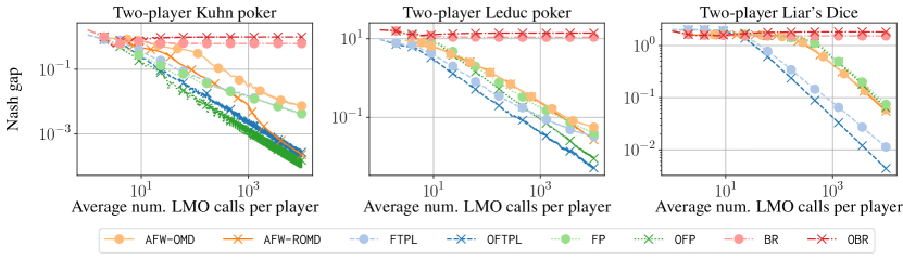
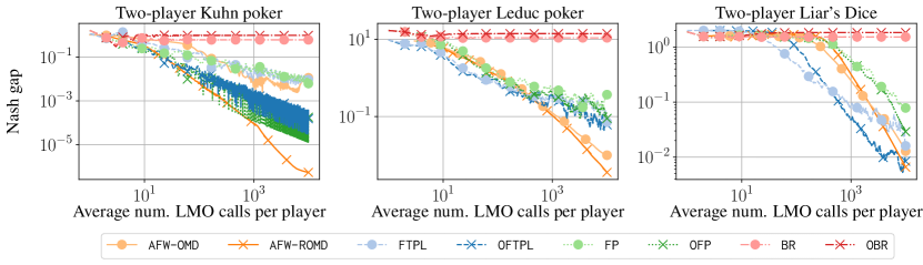
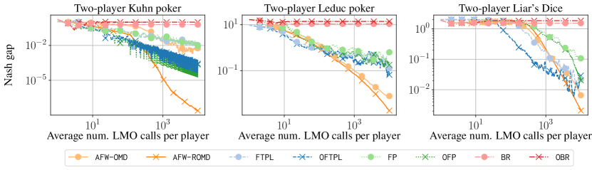
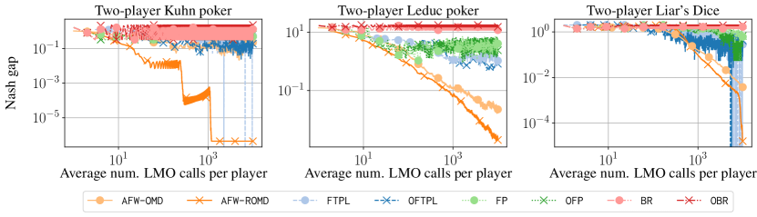
Figure 3: Convergence to NE as a function of average LMO calls per player for , , , , , , , and , for, from top to bottom, uniform, linear, quadratic, and last averaging, without using restarting.

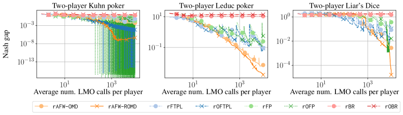
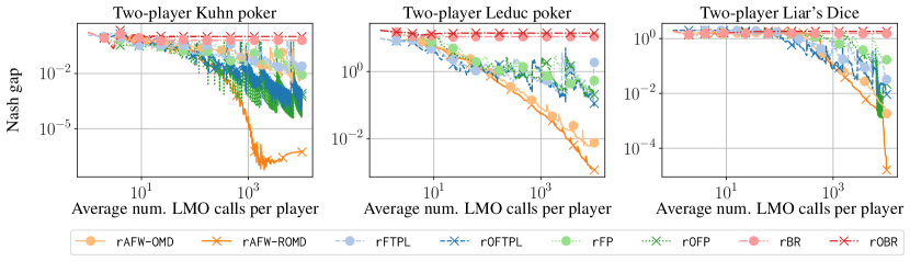
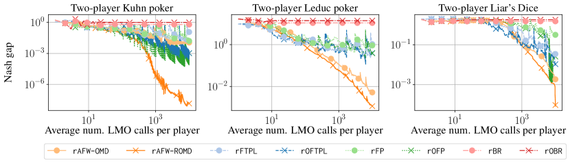
Figure 4: Convergence to NE as a function of average LMO calls per player for , , , , , , , and , for, from top to bottom, uniform, linear, and quadratic averaging, when using restarting.

Appendix H Additional Experimental Details

H.1 Comparisons of Algorithms across Averaging and Restarting Schemes

In this section, we present plots of all the algorithms that we evaluate for different choices of averaging and restarting. This is only relevant for two-player games since, in the other settings, our performance measure is the maximum (uniform) average of an individual player’s regret (so iterate averaging is not relevant).

We implement adaptive restarting by resetting the averaging process every time the duality gap halves. Adaptive restarting was recently shown effective in practice for EFGs [Chakrabarti et al., 2023]. Since adaptive restarting is applied as a heuristic in our experiments that has not previously applied to the algorithms we present as well as the ones we compare against, we label restarted variants of algorithms with a prepended “r” (e.g., the adaptive restarting heuristic applied to is labeled as ) to distinguish them from the original presentation of the algorithm.

In Figure 3, we compare the algorithm on different choices of averaging for all algorithms when restarting is not used. In Figure 4, we compare the algorithm on different choices of averaging for all algorithms when restarting is used.

It can be seen that our algorithms are generally much more stable when averaging or restarting is applied relative to the other algorithms. This is to be expected because while our algorithm has last-iterate convergence guarantees, the other algorithms do not. Thus, even though (O)FTPL and (O)FP seem to perform well in the last-iterate case or with restarting on Kuhn and Liar’s Dice, their behavior is extremely erratic. Observe that our algorithms generally outperform the other algorithms across different averaging and restarting schemes, on Leduc and Liar’s Dice. As mentioned before, (O)FTPL and (O)FP appear to be very unstable, and in Kuhn, while they are often able to find low duality gap solutions, they oscillate quite a bit.

Figure 5: Convergence to NE as a function of average LMO calls per player for for all combinations of averaging schemes and restarting.

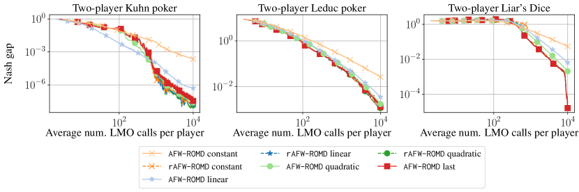
Figure 6: Convergence to NE as a function of average LMO calls per player for for all combinations of averaging schemes and restarting.

H.2 Comparison of Averaging Schemes for and

In Figures 5 and 6, we evaluate and on two-player games on all combinations of averaging and restarting. As above, we label restarted variants of algorithms with a prepended “r” to distinguish them from the original presentation of the algorithm.

We observe here that for , the restarted schemes (whether they are using uniform averaging, linear averaging, or quadratic averaging) are all very similar and generally perform best.

For , we observe that the restarted schemes and the last iterate perform quite similarly and generally better than the non-restarted schemes.

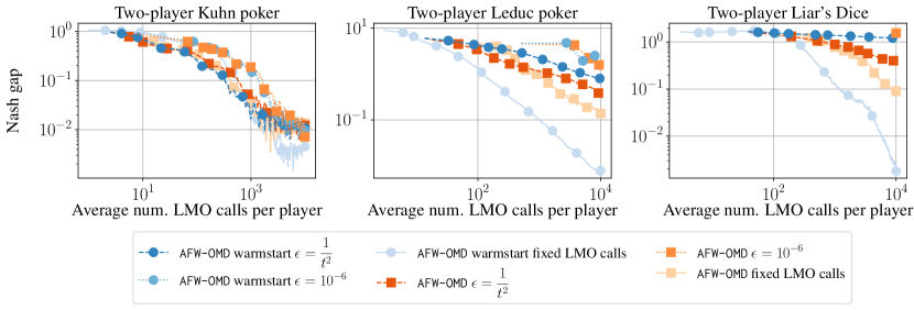
Figure 7: Convergence to NE as a function of average LMO calls per player for for different choices of warmstarting and termination criteria.

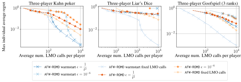
Figure 8: Convergence to CCE as a function of average LMO calls per player for for different choices of warmstarting and termination criteria.

H.3 Comparison of Warmstart and Termination Criteria

In Figure 7, we evaluate on two-player games, and in Figure 8, we evaluate on multiplayer games, when using different combinations of warmstarting and termination criteria for calls, since these combinations were not explored in Section 5. We choose the best averaging scheme for each warm starting and termination criteria combination.

It is quite clear from these figures that warmstarting and using a fixed number of LMO calls per iteration leads to the best performance of our algorithms.

H.4 Parameter Choices

In Tables LABEL:table:NE_no_restarts to LABEL:table:CCE_ablation_optimistic, for each figure presented on experimental results, we provide the specific parameter choices used for each algorithm. The columns, in order, correspond to the game, the algorithm, the averaging scheme, whether restarting was used or not, the max number of LMO calls allowed during each iteration of the algorithm, the stepsize or noise (the latter in the case of and , and the former in all other cases), whether warmstarting was used (for our algorithms), and the APO termination criterion (for our algorithms).

Table 2: The parameters for all algorithms shown in Figure 1 for two-player games. The final two columns are irrelevant for algorithms that are not ours and thus are marked as N/A. Additionally, if the number of LMO calls is not fixed for our algorithms, then N/A is used in the maximum number of LMO calls per iteration ($m$) column.

Game	Algorithm	Averaging	Restarts	$m$	$\eta$	Warmstart	APO term. crit.
Two-player Kuhn poker		quadratic	no	1	0.08	yes	fixed LMO calls
		quadratic	no	5	1.28	yes	fixed LMO calls
		last	no	3	20.48	N/A	N/A
		last	no	3	20.48	N/A	N/A
		constant	no	1	1.28	N/A	N/A
		linear	no	1	1.28	N/A	N/A
		quadratic	no	1	1.28	N/A	N/A
		quadratic	no	1	1.28	N/A	N/A
Two-player Leduc poker		quadratic	no	3	1.28	yes	fixed LMO calls
		last	no	2	1.28	yes	fixed LMO calls
		constant	no	1	0.32	N/A	N/A
		constant	no	1	0.01	N/A	N/A
		constant	no	1	1.28	N/A	N/A
		constant	no	1	1.28	N/A	N/A
		quadratic	no	1	1.28	N/A	N/A
		linear	no	1	1.28	N/A	N/A
Two-player Liar’s Dice		last	no	3	10.24	yes	fixed LMO calls
		last	no	3	10.24	yes	fixed LMO calls
		last	no	1	0.32	N/A	N/A
		last	no	1	0.08	N/A	N/A
		constant	no	1	1.28	N/A	N/A
		linear	no	1	1.28	N/A	N/A
		last	no	1	1.28	N/A	N/A
		last	no	1	1.28	N/A	N/A
table]table:NE_no_restarts

Table 3: The parameters for all algorithms shown in Figure 1 for multiplayer games. The final two columns are irrelevant for algorithms that are not ours and thus are marked as N/A. Additionally, if the number of LMO calls is not fixed for our algorithms, then N/A is used in the maximum number of LMO calls per iteration ($m$) column.

Game	Algorithm	Averaging	Restarts	$m$	$\eta$	Warmstart	APO term. crit.
Three-player Kuhn poker		constant	no	4	40.96	yes	fixed LMO calls
		constant	no	5	1.28	yes	fixed LMO calls
		constant	no	2	0.02	N/A	N/A
		constant	no	2	0.01	N/A	N/A
		constant	no	1	1.28	N/A	N/A
		constant	no	1	1.28	N/A	N/A
		constant	no	1	1.28	N/A	N/A
		constant	no	1	1.28	N/A	N/A
Three-player Liar’s Dice		constant	no	20	40.96	yes	fixed LMO calls
		constant	no	4	20.48	yes	fixed LMO calls
		constant	no	1	0.01	N/A	N/A
		constant	no	1	0.01	N/A	N/A
		constant	no	1	1.28	N/A	N/A
		constant	no	1	1.28	N/A	N/A
		constant	no	1	1.28	N/A	N/A
		constant	no	1	1.28	N/A	N/A
Three-player Goofspiel (3 ranks)		constant	no	1	81.92	yes	fixed LMO calls
		constant	no	2	40.96	yes	fixed LMO calls
		constant	no	1	0.04	N/A	N/A
		constant	no	2	0.04	N/A	N/A
		constant	no	1	1.28	N/A	N/A
		constant	no	1	1.28	N/A	N/A
		constant	no	1	1.28	N/A	N/A
		constant	no	1	1.28	N/A	N/A
table]table:CCE

Table 4: The parameters for all algorithms shown in Figure 2 for two-player games. The final two columns are irrelevant for algorithms that are not ours and thus are marked as N/A. Additionally, if the number of LMO calls is not fixed for our algorithms, then N/A is used in the maximum number of LMO calls per iteration ($m$) column.

Game	Algorithm	Averaging	Restarts	$m$	$\eta$	Warmstart	APO term. crit.
Two-player Kuhn poker		quadratic	no	N/A	1.28	yes	$\epsilon=\frac{1}{t^{2}}$
		quadratic	no	N/A	1.28	yes	$\epsilon=10^{-6}$
		quadratic	no	5	1.28	yes	fixed LMO calls
		last	no	N/A	1.28	no	$\epsilon=\frac{1}{t^{2}}$
		last	no	N/A	1.28	no	$\epsilon=10^{-6}$
		last	no	20	1.28	no	fixed LMO calls
Two-player Leduc poker		last	no	N/A	0.64	yes	$\epsilon=\frac{1}{t^{2}}$
		last	no	N/A	2.56	yes	$\epsilon=10^{-6}$
		last	no	3	1.28	yes	fixed LMO calls
		last	no	N/A	0.64	no	$\epsilon=\frac{1}{t^{2}}$
		last	no	N/A	2.56	no	$\epsilon=10^{-6}$
		quadratic	no	100	0.64	no	fixed LMO calls
Two-player Liar’s Dice		last	no	N/A	5.12	yes	$\epsilon=\frac{1}{t^{2}}$
		quadratic	no	N/A	5.12	yes	$\epsilon=10^{-6}$
		last	no	3	10.24	yes	fixed LMO calls
		last	no	N/A	5.12	no	$\epsilon=\frac{1}{t^{2}}$
		quadratic	no	N/A	0.04	no	$\epsilon=10^{-6}$
		last	no	200	5.12	no	fixed LMO calls
table]table:NE_no_restarts_ablation

Table 5: The parameters for all algorithms shown in Figure 2 for multiplayer games. The final two columns are irrelevant for algorithms that are not ours and thus are marked as N/A. Additionally, if the number of LMO calls is not fixed for our algorithms, then N/A is used in the maximum number of LMO calls per iteration ($m$) column.

Game	Algorithm	Averaging	Restarts	$m$	$\eta$	Warmstart	APO term. crit.
Three-player Kuhn poker		constant	no	N/A	40.96	yes	$\epsilon=\frac{1}{t^{2}}$
		constant	no	N/A	40.96	yes	$\epsilon=10^{-6}$
		constant	no	4	40.96	yes	fixed LMO calls
		constant	no	N/A	81.92	no	$\epsilon=\frac{1}{t^{2}}$
		constant	no	N/A	40.96	no	$\epsilon=10^{-6}$
		constant	no	1	40.96	no	fixed LMO calls
Three-player Liar’s Dice		constant	no	N/A	40.96	yes	$\epsilon=\frac{1}{t^{2}}$
		constant	no	N/A	0.04	yes	$\epsilon=10^{-6}$
		constant	no	20	40.96	yes	fixed LMO calls
		constant	no	N/A	40.96	no	$\epsilon=\frac{1}{t^{2}}$
		constant	no	N/A	0.02	no	$\epsilon=10^{-6}$
		constant	no	100	40.96	no	fixed LMO calls
Three-player Goofspiel (3 ranks)		constant	no	N/A	40.96	yes	$\epsilon=\frac{1}{t^{2}}$
		constant	no	N/A	81.92	yes	$\epsilon=10^{-6}$
		constant	no	1	81.92	yes	fixed LMO calls
		constant	no	N/A	81.92	no	$\epsilon=\frac{1}{t^{2}}$
		constant	no	N/A	81.92	no	$\epsilon=10^{-6}$
		constant	no	20	40.96	no	fixed LMO calls
table]table:CCE_ablation

Table 6: The parameters for all algorithms shown in Figure 3. The final two columns are irrelevant for algorithms that are not ours and thus are marked as N/A. Additionally, if the number of LMO calls is not fixed for our algorithms, then N/A is used in the maximum number of LMO calls per iteration ($m$) column.

Game	Algorithm	Averaging	Restarts	$m$	$\eta$	Warmstart	APO term. crit.
Two-player Kuhn poker		constant	no	3	0.32	yes	fixed LMO calls
		constant	no	4	1.28	yes	fixed LMO calls
		constant	no	1	0.04	N/A	N/A
		constant	no	1	0.08	N/A	N/A
		constant	no	1	1.28	N/A	N/A
		constant	no	1	1.28	N/A	N/A
		constant	no	1	1.28	N/A	N/A
		constant	no	1	1.28	N/A	N/A
Two-player Leduc poker		constant	no	3	2.56	yes	fixed LMO calls
		constant	no	3	1.28	yes	fixed LMO calls
		constant	no	1	0.32	N/A	N/A
		constant	no	1	0.01	N/A	N/A
		constant	no	1	1.28	N/A	N/A
		constant	no	1	1.28	N/A	N/A
		constant	no	1	1.28	N/A	N/A
		constant	no	1	1.28	N/A	N/A
Two-player Liar’s Dice		constant	no	3	10.24	yes	fixed LMO calls
		constant	no	2	5.12	yes	fixed LMO calls
		constant	no	1	0.02	N/A	N/A
		constant	no	1	0.01	N/A	N/A
		constant	no	1	1.28	N/A	N/A
		constant	no	1	1.28	N/A	N/A
		constant	no	1	1.28	N/A	N/A
		constant	no	1	1.28	N/A	N/A
Two-player Kuhn poker		linear	no	1	0.32	yes	fixed LMO calls
		linear	no	2	2.56	yes	fixed LMO calls
		linear	no	1	0.64	N/A	N/A
		linear	no	1	0.04	N/A	N/A
		linear	no	1	1.28	N/A	N/A
		linear	no	1	1.28	N/A	N/A
		linear	no	1	1.28	N/A	N/A
		linear	no	1	1.28	N/A	N/A
Two-player Leduc poker		linear	no	3	1.28	yes	fixed LMO calls
		linear	no	5	1.28	yes	fixed LMO calls
		linear	no	1	0.32	N/A	N/A
		linear	no	1	0.08	N/A	N/A
		linear	no	1	1.28	N/A	N/A
		linear	no	1	1.28	N/A	N/A
		linear	no	1	1.28	N/A	N/A
		linear	no	1	1.28	N/A	N/A
Two-player Liar’s Dice		linear	no	3	10.24	yes	fixed LMO calls
		linear	no	2	10.24	yes	fixed LMO calls
		linear	no	1	0.02	N/A	N/A
		linear	no	2	0.08	N/A	N/A
		linear	no	1	1.28	N/A	N/A
		linear	no	1	1.28	N/A	N/A
		linear	no	1	1.28	N/A	N/A
		linear	no	1	1.28	N/A	N/A
Two-player Kuhn poker		quadratic	no	1	0.08	yes	fixed LMO calls
		quadratic	no	5	1.28	yes	fixed LMO calls
		quadratic	no	1	0.32	N/A	N/A
		quadratic	no	1	0.04	N/A	N/A
		quadratic	no	1	1.28	N/A	N/A
		quadratic	no	1	1.28	N/A	N/A
		quadratic	no	1	1.28	N/A	N/A
		quadratic	no	1	1.28	N/A	N/A
Two-player Leduc poker		quadratic	no	3	1.28	yes	fixed LMO calls
		quadratic	no	3	1.28	yes	fixed LMO calls
		quadratic	no	1	0.32	N/A	N/A
		quadratic	no	1	0.16	N/A	N/A
		quadratic	no	1	1.28	N/A	N/A
		quadratic	no	1	1.28	N/A	N/A
		quadratic	no	1	1.28	N/A	N/A
		quadratic	no	1	1.28	N/A	N/A
Two-player Liar’s Dice		quadratic	no	2	10.24	yes	fixed LMO calls
		quadratic	no	2	10.24	yes	fixed LMO calls
		quadratic	no	1	0.32	N/A	N/A
		quadratic	no	1	0.08	N/A	N/A
		quadratic	no	1	1.28	N/A	N/A
		quadratic	no	1	1.28	N/A	N/A
		quadratic	no	1	1.28	N/A	N/A
		quadratic	no	1	1.28	N/A	N/A
Two-player Kuhn poker		last	no	1	0.32	yes	fixed LMO calls
		last	no	2	2.56	yes	fixed LMO calls
		last	no	3	20.48	N/A	N/A
		last	no	20	0.32	N/A	N/A
		last	no	1	1.28	N/A	N/A
		last	no	1	1.28	N/A	N/A
		last	no	1	1.28	N/A	N/A
		last	no	1	1.28	N/A	N/A
Two-player Leduc poker		last	no	1	1.28	yes	fixed LMO calls
		last	no	2	1.28	yes	fixed LMO calls
		last	no	10	2.56	N/A	N/A
		last	no	200	0.16	N/A	N/A
		last	no	1	1.28	N/A	N/A
		last	no	1	1.28	N/A	N/A
		last	no	1	1.28	N/A	N/A
		last	no	1	1.28	N/A	N/A
Two-player Liar’s Dice		last	no	4	5.12	yes	fixed LMO calls
		last	no	3	10.24	yes	fixed LMO calls
		last	no	1	0.32	N/A	N/A
		last	no	2	0.02	N/A	N/A
		last	no	1	1.28	N/A	N/A
		last	no	1	1.28	N/A	N/A
		last	no	1	1.28	N/A	N/A
		last	no	1	1.28	N/A	N/A
table]table:NE_avg_comparison_no_restarts

Table 7: The parameters for all algorithms shown in Figure 4. The final two columns are irrelevant for algorithms that are not ours and thus are marked as N/A. Additionally, if the number of LMO calls is not fixed for our algorithms, then N/A is used in the maximum number of LMO calls per iteration ($m$) column.

Game	Algorithm	Averaging	Restarts	$m$	$\eta$	Warmstart	APO term. crit.
Two-player Kuhn poker		constant	yes	4	0.32	yes	fixed LMO calls
		constant	yes	5	1.28	yes	fixed LMO calls
		constant	yes	1	5.12	N/A	N/A
		constant	yes	1	0.01	N/A	N/A
		constant	yes	1	1.28	N/A	N/A
		constant	yes	1	1.28	N/A	N/A
		constant	yes	1	1.28	N/A	N/A
		constant	yes	1	1.28	N/A	N/A
Two-player Leduc poker		constant	yes	3	1.28	yes	fixed LMO calls
		constant	yes	4	1.28	yes	fixed LMO calls
		constant	yes	1	0.64	N/A	N/A
		constant	yes	2	0.16	N/A	N/A
		constant	yes	1	1.28	N/A	N/A
		constant	yes	1	1.28	N/A	N/A
		constant	yes	1	1.28	N/A	N/A
		constant	yes	1	1.28	N/A	N/A
Two-player Liar’s Dice		constant	yes	2	10.24	yes	fixed LMO calls
		constant	yes	3	10.24	yes	fixed LMO calls
		constant	yes	1	0.08	N/A	N/A
		constant	yes	2	0.02	N/A	N/A
		constant	yes	1	1.28	N/A	N/A
		constant	yes	1	1.28	N/A	N/A
		constant	yes	1	1.28	N/A	N/A
		constant	yes	1	1.28	N/A	N/A
Two-player Kuhn poker		linear	yes	4	0.32	yes	fixed LMO calls
		linear	yes	2	2.56	yes	fixed LMO calls
		linear	yes	1	0.08	N/A	N/A
		linear	yes	2	0.04	N/A	N/A
		linear	yes	1	1.28	N/A	N/A
		linear	yes	1	1.28	N/A	N/A
		linear	yes	1	1.28	N/A	N/A
		linear	yes	1	1.28	N/A	N/A
Two-player Leduc poker		linear	yes	3	1.28	yes	fixed LMO calls
		linear	yes	3	1.28	yes	fixed LMO calls
		linear	yes	1	0.32	N/A	N/A
		linear	yes	1	0.01	N/A	N/A
		linear	yes	1	1.28	N/A	N/A
		linear	yes	1	1.28	N/A	N/A
		linear	yes	1	1.28	N/A	N/A
		linear	yes	1	1.28	N/A	N/A
Two-player Liar’s Dice		linear	yes	2	10.24	yes	fixed LMO calls
		linear	yes	3	10.24	yes	fixed LMO calls
		linear	yes	2	0.16	N/A	N/A
		linear	yes	1	0.16	N/A	N/A
		linear	yes	1	1.28	N/A	N/A
		linear	yes	1	1.28	N/A	N/A
		linear	yes	1	1.28	N/A	N/A
		linear	yes	1	1.28	N/A	N/A
Two-player Kuhn poker		quadratic	yes	3	0.64	yes	fixed LMO calls
		quadratic	yes	5	1.28	yes	fixed LMO calls
		quadratic	yes	1	0.08	N/A	N/A
		quadratic	yes	3	0.04	N/A	N/A
		quadratic	yes	1	1.28	N/A	N/A
		quadratic	yes	1	1.28	N/A	N/A
		quadratic	yes	1	1.28	N/A	N/A
		quadratic	yes	1	1.28	N/A	N/A
Two-player Leduc poker		quadratic	yes	2	1.28	yes	fixed LMO calls
		quadratic	yes	3	1.28	yes	fixed LMO calls
		quadratic	yes	1	0.32	N/A	N/A
		quadratic	yes	1	0.32	N/A	N/A
		quadratic	yes	1	1.28	N/A	N/A
		quadratic	yes	1	1.28	N/A	N/A
		quadratic	yes	1	1.28	N/A	N/A
		quadratic	yes	1	1.28	N/A	N/A
Two-player Liar’s Dice		quadratic	yes	2	10.24	yes	fixed LMO calls
		quadratic	yes	2	10.24	yes	fixed LMO calls
		quadratic	yes	1	0.32	N/A	N/A
		quadratic	yes	1	0.16	N/A	N/A
		quadratic	yes	1	1.28	N/A	N/A
		quadratic	yes	1	1.28	N/A	N/A
		quadratic	yes	1	1.28	N/A	N/A
		quadratic	yes	1	1.28	N/A	N/A
table]table:NE_avg_comparison_restarts

Table 8: The parameters for all algorithms shown in Figure 5. The final two columns are irrelevant for algorithms that are not ours and thus are marked as N/A. Additionally, if the number of LMO calls is not fixed for our algorithms, then N/A is used in the maximum number of LMO calls per iteration ($m$) column.

Game	Algorithm	Averaging	Restarts	$m$	$\eta$	Warmstart	APO term. crit.
Two-player Kuhn poker		constant	no	1	0.32	yes	fixed LMO calls
		constant	yes	1	0.32	yes	fixed LMO calls
		linear	no	1	0.08	yes	fixed LMO calls
		linear	yes	1	0.32	yes	fixed LMO calls
		quadratic	no	5	0.32	yes	fixed LMO calls
		quadratic	yes	1	0.32	yes	fixed LMO calls
		last	no	1	0.32	yes	fixed LMO calls
Two-player Leduc poker		constant	no	3	1.28	yes	fixed LMO calls
		constant	yes	3	0.64	yes	fixed LMO calls
		linear	no	3	1.28	yes	fixed LMO calls
		linear	yes	3	0.64	yes	fixed LMO calls
		quadratic	no	3	1.28	yes	fixed LMO calls
		quadratic	yes	3	0.64	yes	fixed LMO calls
		last	no	4	0.64	yes	fixed LMO calls
Two-player Liar’s Dice		constant	no	3	10.24	yes	fixed LMO calls
		constant	yes	3	10.24	yes	fixed LMO calls
		linear	no	2	10.24	yes	fixed LMO calls
		linear	yes	2	10.24	yes	fixed LMO calls
		quadratic	no	2	10.24	yes	fixed LMO calls
		quadratic	yes	2	10.24	yes	fixed LMO calls
		last	no	3	10.24	yes	fixed LMO calls
table]table:NE_ablation_averaging_no_optimistic

Table 9: The parameters for all algorithms shown in Figure 6. The final two columns are irrelevant for algorithms that are not ours and thus are marked as N/A. Additionally, if the number of LMO calls is not fixed for our algorithms, then N/A is used in the maximum number of LMO calls per iteration ($m$) column.

Game	Algorithm	Averaging	Restarts	$m$	$\eta$	Warmstart	APO term. crit.
Two-player Kuhn poker		constant	no	4	1.28	yes	fixed LMO calls
		constant	yes	N/A	1.28	yes	$\epsilon=\frac{1}{t^{2}}$
		linear	no	2	2.56	yes	fixed LMO calls
		linear	yes	N/A	1.28	yes	$\epsilon=\frac{1}{t^{2}}$
		quadratic	no	N/A	1.28	yes	$\epsilon=\frac{1}{t^{2}}$
		quadratic	yes	N/A	1.28	yes	$\epsilon=\frac{1}{t^{2}}$
		last	no	N/A	1.28	yes	$\epsilon=\frac{1}{t^{2}}$
Two-player Leduc poker		constant	no	3	1.28	yes	fixed LMO calls
		constant	yes	3	1.28	yes	fixed LMO calls
		linear	no	3	1.28	yes	fixed LMO calls
		linear	yes	3	1.28	yes	fixed LMO calls
		quadratic	no	5	1.28	yes	fixed LMO calls
		quadratic	yes	3	1.28	yes	fixed LMO calls
		last	no	3	1.28	yes	fixed LMO calls
Two-player Liar’s Dice		constant	no	2	5.12	yes	fixed LMO calls
		constant	yes	3	10.24	yes	fixed LMO calls
		linear	no	2	10.24	yes	fixed LMO calls
		linear	yes	3	10.24	yes	fixed LMO calls
		quadratic	no	2	10.24	yes	fixed LMO calls
		quadratic	yes	3	10.24	yes	fixed LMO calls
		last	no	3	10.24	yes	fixed LMO calls
table]table:NE_ablation_averaging_optimistic

Table 10: The parameters for all algorithms shown in Figure 7. The final two columns are irrelevant for algorithms that are not ours and thus are marked as N/A. Additionally, if the number of LMO calls is not fixed for our algorithms, then N/A is used in the maximum number of LMO calls per iteration ($m$) column.

Game	Algorithm	Averaging	Restarts	$m$	$\eta$	Warmstart	APO term. crit.
Two-player Kuhn poker		linear	no	N/A	0.64	yes	$\epsilon=\frac{1}{t^{2}}$
		linear	no	N/A	0.64	yes	$\epsilon=10^{-6}$
		linear	no	1	0.08	yes	fixed LMO calls
		linear	no	N/A	0.64	no	$\epsilon=\frac{1}{t^{2}}$
		linear	no	N/A	0.64	no	$\epsilon=10^{-6}$
		linear	no	10	0.64	no	fixed LMO calls
Two-player Leduc poker		quadratic	no	N/A	2.56	yes	$\epsilon=\frac{1}{t^{2}}$
		last	no	N/A	10.24	yes	$\epsilon=10^{-6}$
		quadratic	no	3	1.28	yes	fixed LMO calls
		quadratic	no	N/A	2.56	no	$\epsilon=\frac{1}{t^{2}}$
		last	no	N/A	5.12	no	$\epsilon=10^{-6}$
		quadratic	no	100	2.56	no	fixed LMO calls
Two-player Liar’s Dice		linear	no	N/A	20.48	yes	$\epsilon=\frac{1}{t^{2}}$
		last	no	N/A	0.64	yes	$\epsilon=10^{-6}$
		last	no	3	10.24	yes	fixed LMO calls
		linear	no	N/A	20.48	no	$\epsilon=\frac{1}{t^{2}}$
		linear	no	N/A	0.02	no	$\epsilon=10^{-6}$
		quadratic	no	200	10.24	no	fixed LMO calls
table]table:NE_no_restarts_ablation_no_optimistic

Table 11: The parameters for all algorithms shown in Figure 8. The final two columns are irrelevant for algorithms that are not ours and thus are marked as N/A. Additionally, if the number of LMO calls is not fixed for our algorithms, then N/A is used in the maximum number of LMO calls per iteration ($m$) column.

Game	Algorithm	Averaging	Restarts	$m$	$\eta$	Warmstart	APO term. crit.
Three-player Kuhn poker		constant	no	N/A	1.28	yes	$\epsilon=\frac{1}{t^{2}}$
		constant	no	N/A	1.28	yes	$\epsilon=10^{-6}$
		constant	no	5	1.28	yes	fixed LMO calls
		constant	no	N/A	1.28	no	$\epsilon=\frac{1}{t^{2}}$
		constant	no	N/A	1.28	no	$\epsilon=10^{-6}$
		constant	no	4	1.28	no	fixed LMO calls
Three-player Liar’s Dice		constant	no	N/A	5.12	yes	$\epsilon=\frac{1}{t^{2}}$
		constant	no	N/A	0.02	yes	$\epsilon=10^{-6}$
		constant	no	20	10.24	yes	fixed LMO calls
		constant	no	N/A	10.24	no	$\epsilon=\frac{1}{t^{2}}$
		constant	no	N/A	20.48	no	$\epsilon=10^{-6}$
		constant	no	100	5.12	no	fixed LMO calls
Three-player Goofspiel (3 ranks)		constant	no	N/A	20.48	yes	$\epsilon=\frac{1}{t^{2}}$
		constant	no	N/A	40.96	yes	$\epsilon=10^{-6}$
		constant	no	2	40.96	yes	fixed LMO calls
		constant	no	N/A	20.48	no	$\epsilon=\frac{1}{t^{2}}$
		constant	no	N/A	40.96	no	$\epsilon=10^{-6}$
		constant	no	100	20.48	no	fixed LMO calls
table]table:CCE_ablation_optimistic

References

• Abernethy et al. (2016) Jacob Abernethy, Chansoo Lee, and Ambuj Tewari. Perturbation techniques in online learning and optimization. Perturbations, Optimization, and Statistics, 233, 2016.
• Anagnostides et al. (2022a) Ioannis Anagnostides, Gabriele Farina, Christian Kroer, Chung-Wei Lee, Haipeng Luo, and Tuomas Sandholm. Uncoupled learning dynamics with ${O}(\mathop{{\rm log}}{T})$ swap regret in multiplayer games. In Neural Information Processing Systems (NeurIPS), 2022a.
• Anagnostides et al. (2022b) Ioannis Anagnostides, Ioannis Panageas, Gabriele Farina, and Tuomas Sandholm. On last-iterate convergence beyond zero-sum games. In International Conference on Machine Learning (ICML), 2022b.
• Anagnostides et al. (2023) Ioannis Anagnostides, Gabriele Farina, and Tuomas Sandholm. Near-optimal $\Phi$-regret learning in extensive-form games. In International Conference on Machine Learning (ICML), 2023.
• Applegate et al. (2023) David Applegate, Oliver Hinder, Haihao Lu, and Miles Lubin. Faster first-order primal-dual methods for linear programming using restarts and sharpness. Mathematical Programming, 201(1-2):133–184, 2023.
• Bashiri and Zhang (2017) Mohammad Ali Bashiri and Xinhua Zhang. Decomposition-invariant conditional gradient for general polytopes with line search. In Neural Information Processing Systems (NIPS), 2017.
• Beck and Shtern (2017) Amir Beck and Shimrit Shtern. Linearly convergent away-step conditional gradient for non-strongly convex functions. Mathematical Programming, 164:1–27, 2017.
• Bomze et al. (2021) Immanuel M. Bomze, Francesco Rinaldi, and Damiano Zeffiro. Frank–Wolfe and friends: a journey into projection-free first-order optimization methods. 4OR, 19:313–345, 2021.
• Bowling et al. (2015) Michael Bowling, Neil Burch, Michael Johanson, and Oskari Tammelin. Heads-up limit hold’em poker is solved. Science, 347(6218):145–149, 2015.
• Braun et al. (2022) Gábor Braun, Alejandro Carderera, Cyrille W. Combettes, Hamed Hassani, Amin Karbasi, Aryan Mokhtari, and Sebastian Pokutta. Conditional gradient methods. arXiv preprint arXiv:2211.14103, 2022.
• Brown (1951) George W. Brown. Iterative solution of games by fictitious play. Activity Analysis of Production and Allocation, 13(1):374, 1951.
• Brown and Sandholm (2018) Noam Brown and Tuomas Sandholm. Superhuman AI for heads-up no-limit poker: Libratus beats top professionals. Science, 359(6374):418–424, 2018.
• Brown and Sandholm (2019a) Noam Brown and Tuomas Sandholm. Solving imperfect-information games via discounted regret minimization. In AAAI Conference on Artificial Intelligence (AAAI), 2019a.
• Brown and Sandholm (2019b) Noam Brown and Tuomas Sandholm. Superhuman AI for multiplayer poker. Science, 365(6456):885–890, 2019b.
• Chakrabarti et al. (2023) Darshan Chakrabarti, Jelena Diakonikolas, and Christian Kroer. Block-coordinate methods and restarting for solving extensive-form games. arXiv preprint arXiv:2307.16754, 2023.
• Daskalakis and Pan (2014) Constantinos Daskalakis and Qinxuan Pan. A counter-example to Karlin’s strong conjecture for fictitious play. In IEEE Annual Symposium on Foundations of Computer Science (FOCS), 2014.
• Daskalakis et al. (2015) Constantinos Daskalakis, Alan Deckelbaum, and Anthony Kim. Near-optimal no-regret algorithms for zero-sum games. Games and Economic Behavior, 92:327–348, 2015.
• Daskalakis et al. (2021) Constantinos Daskalakis, Maxwell Fishelson, and Noah Golowich. Near-optimal no-regret learning in general games. In Neural Information Processing Systems (NeurIPS), 2021.
• Farina et al. (2018) Gabriele Farina, Andrea Celli, Nicola Gatti, and Tuomas Sandholm. Ex ante coordination and collusion in zero-sum multi-player extensive-form games. In Neural Information Processing Systems (NeurIPS), 2018.
• Farina et al. (2021a) Gabriele Farina, Christian Kroer, and Tuomas Sandholm. Better regularization for sequential decision spaces: Fast convergence rates for Nash, correlated, and team equilibria. In ACM Conference on Economics and Computation (EC), 2021a.
• Farina et al. (2021b) Gabriele Farina, Christian Kroer, and Tuomas Sandholm. Faster game solving via predictive Blackwell approachability: Connecting regret matching and mirror descent. In AAAI Conference on Artificial Intelligence (AAAI), 2021b.
• Farina et al. (2022a) Gabriele Farina, Ioannis Anagnostides, Haipeng Luo, Chung-Wei Lee, Christian Kroer, and Tuomas Sandholm. Near-optimal no-regret learning dynamics for general convex games. In Neural Information Processing Systems (NeurIPS), 2022a.
• Farina et al. (2022b) Gabriele Farina, Chung-Wei Lee, Haipeng Luo, and Christian Kroer. Kernelized multiplicative weights for 0/1-polyhedral games: Bridging the gap between learning in extensive-form and normal-form games. In International Conference on Machine Learning (ICML), 2022b.
• Fercoq (2023) Olivier Fercoq. Quadratic error bound of the smoothed gap and the restarted averaged primal-dual hybrid gradient. arXiv preprint arXiv:2206.03041, 2023.
• Frank and Wolfe (1956) Marguerite Frank and Philip Wolfe. An algorithm for quadratic programming. Naval Research Logistics Quarterly, 3(1-2):95–110, 1956.
• Gao et al. (2021) Yuan Gao, Christian Kroer, and Donald Goldfarb. Increasing iterate averaging for solving saddle-point problems. In AAAI Conference on Artificial Intelligence (AAAI), 2021.
• Garber and Hazan (2015) Dan Garber and Elad Hazan. Faster rates for the Frank-Wolfe method over strongly-convex sets. In International Conference on Machine Learning (ICML), 2015.
• Garber and Meshi (2016) Dan Garber and Ofer Meshi. Linear-memory and decomposition-invariant linearly convergent conditional gradient algorithm for structured polytopes. In Neural Information Processing Systems (NIPS), 2016.
• Gidel et al. (2017) Gauthier Gidel, Tony Jebara, and Simon Lacoste-Julien. Frank-Wolfe algorithms for saddle point problems. In Artificial Intelligence and Statistics (AISTATS), 2017.
• Gilpin et al. (2012) Andrew Gilpin, Javier Peña, and Tuomas Sandholm. First-order algorithm with $\mathcal{O}(\mathrm{ln}(1/\epsilon))$ convergence for $\epsilon$-equilibrium in two-person zero-sum games. Mathematical Programming, 133(1):279–298, 2012.
• Guélat and Marcotte (1986) Jacques Guélat and Patrice Marcotte. Some comments on Wolfe’s ‘away step’. Mathematical Programming, 35(1):110–119, 1986.
• Hazan and Kale (2012) Elad Hazan and Satyen Kale. Projection-free online learning. In International Coference on Machine Learning (ICML), 2012.
• Hazan et al. (2016) Elad Hazan et al. Introduction to online convex optimization. Foundations and Trends® in Optimization, 2(3-4):157–325, 2016.
• Hoda et al. (2010) Samid Hoda, Andrew Gilpin, Javier Pena, and Tuomas Sandholm. Smoothing techniques for computing Nash equilibria of sequential games. Mathematics of Operations Research, 35(2):494–512, 2010.
• Jaggi (2013) Martin Jaggi. Revisiting Frank-Wolfe: Projection-free sparse convex optimization. In International Conference on Machine Learning (ICML), 2013.
• Joulani et al. (2017) Pooria Joulani, András György, and Csaba Szepesvári. A modular analysis of adaptive (non-)convex optimization: Optimism, composite objectives, and variational bounds. In International Conference on Algorithmic Learning Theory (ALT), 2017.
• Kalai and Vempala (2005) Adam Kalai and Santosh Vempala. Efficient algorithms for online decision problems. Journal of Computer and System Sciences, 71(3):291–307, 2005.
• Karimi et al. (2016) Hamed Karimi, Julie Nutini, and Mark Schmidt. Linear convergence of gradient and proximal-gradient methods under the Polyak-Łojasiewicz condition. In Joint European Conference on Machine Learning and Knowledge Discovery in Databases (ECML PKDD), 2016.
• Koller et al. (1996) Daphne Koller, Nimrod Megiddo, and Bernhard von Stengel. Efficient computation of equilibria for extensive two-person games. Games and Economic Behavior, 14(2):247–259, 1996.
• Kroer et al. (2020) Christian Kroer, Kevin Waugh, Fatma Kılınç-Karzan, and Tuomas Sandholm. Faster algorithms for extensive-form game solving via improved smoothing functions. Mathematical Programming, pages 1–33, 2020.
• Kuhn (1950) Harold W. Kuhn. A simplified two-person poker. Contributions to the Theory of Games, 1:97–103, 1950.
• Lacoste-Julien and Jaggi (2015) Simon Lacoste-Julien and Martin Jaggi. On the global linear convergence of Frank-Wolfe optimization variants. In Neural Information Processing Systems (NIPS), 2015.
• Lan (2016) Guanghui Lan. Gradient sliding for composite optimization. Mathematical Programming, 159:201–235, 2016.
• Lan and Zhou (2016) Guanghui Lan and Yi Zhou. Conditional gradient sliding for convex optimization. SIAM Journal on Optimization, 26(2):1379–1409, 2016.
• Lanctot et al. (2009) Marc Lanctot, Kevin Waugh, Martin Zinkevich, and Michael Bowling. Monte Carlo sampling for regret minimization in extensive games. In Neural Information Processing Systems (NIPS), 2009.
• Lanctot et al. (2017) Marc Lanctot, Vinicius Zambaldi, Audrunas Gruslys, Angeliki Lazaridou, Karl Tuyls, Julien Pérolat, David Silver, and Thore Graepel. A unified game-theoretic approach to multiagent reinforcement learning. In Neural Information Processing Systems (NIPS), 2017.
• Lee et al. (2021) Chung-Wei Lee, Christian Kroer, and Haipeng Luo. Last-iterate convergence in extensive-form games. In Neural Information Processing Systems (NeurIPS), 2021.
• Lisỳ et al. (2015) Viliam Lisỳ, Marc Lanctot, and Michael Bowling. Online Monte Carlo counterfactual regret minimization for search in imperfect information games. In International Conference on Autonomous Agents and Multiagent Systems (AAMAS), 2015.
• Malitsky (2015) Yu Malitsky. Projected reflected gradient methods for monotone variational inequalities. SIAM Journal on Optimization, 25(1):502–520, 2015.
• McMahan et al. (2003) H. Brendan McMahan, Geoffrey J. Gordon, and Avrim Blum. Planning in the presence of cost functions controlled by an adversary. In International Conference on Machine Learning (ICML), 2003.
• Orabona (2019) Francesco Orabona. A modern introduction to online learning. arXiv preprint arXiv:1912.13213, 2019.
• Pena and Rodriguez (2019) Javier Pena and Daniel Rodriguez. Polytope conditioning and linear convergence of the Frank–Wolfe algorithm. Mathematics of Operations Research, 44(1):1–18, 2019.
• Robinson (1951) Julia Robinson. An iterative method of solving a game. Annals of Mathematics, 54(2):296–301, 1951.
• Romanovskii (1962) I.V. Romanovskii. Reduction of a game with full memory to a matrix game. Doklady Akademii Nauk SSSR, 144(1):62–+, 1962.
• Ross (1971) Sheldon M. Ross. Goofspiel — the game of pure strategy. Journal of Applied Probability, 8(3):621–625, 1971.
• Southey et al. (2012) Finnegan Southey, Michael P. Bowling, Bryce Larson, Carmelo Piccione, Neil Burch, Darse Billings, and Chris Rayner. Bayes’ bluff: Opponent modelling in poker. arXiv preprint arXiv:1207.1411, 2012.
• Suggala and Netrapalli (2020) Arun Suggala and Praneeth Netrapalli. Follow the perturbed leader: Optimism and fast parallel algorithms for smooth minimax games. In Neural Information Processing Systems (NeurIPS), 2020.
• Syrgkanis et al. (2015) Vasilis Syrgkanis, Alekh Agarwal, Haipeng Luo, and Robert E Schapire. Fast convergence of regularized learning in games. In Neural Information Processing Systems (NIPS), 2015.
• Tammelin et al. (2015) Oskari Tammelin, Neil Burch, Michael Johanson, and Michael Bowling. Solving heads-up limit Texas hold’em. In International Joint Conference on Artificial Intelligence (IJCAI), 2015.
• Tseng (1995) Paul Tseng. On linear convergence of iterative methods for the variational inequality problem. Journal of Computational and Applied Mathematics, 60(1-2):237–252, 1995.
• von Stengel (1996) Bernhard von Stengel. Efficient computation of behavior strategies. Games and Economic Behavior, 14(2):220–246, 1996.
• Wei et al. (2021) Chen-Yu Wei, Chung-Wei Lee, Mengxiao Zhang, and Haipeng Luo. Linear last-iterate convergence in constrained saddle-point optimization. In International Conference on Learning Representations (ICLR), 2021.
• Wibisono et al. (2022) Andre Wibisono, Molei Tao, and Georgios Piliouras. Alternating mirror descent for constrained min-max games. In Neural Information Processing Systems (NeurIPS), 2022.
• Wolfe (1970) Philip Wolfe. Convergence theory in nonlinear programming. Integer and Nonlinear Programming, pages 1–36, 1970.
• Zinkevich et al. (2007) Martin Zinkevich, Michael Johanson, Michael Bowling, and Carmelo Piccione. Regret minimization in games with incomplete information. In Neural Information Processing Systems (NIPS), 2007.