The Initial Mass Function Based on the Full-sky 20-pc Census of 3,600 Stars and Brown Dwarfs
Abstract
A complete accounting of nearby objects – from the highest-mass white dwarf progenitors down to low-mass brown dwarfs – is now possible, thanks to an almost complete set of trigonometric parallax determinations from Gaia, ground-based surveys, and Spitzer follow-up. We create a census of objects within a Sun-centered sphere of 20-pc radius and check published literature to decompose each binary or higher-order system into its separate components. The result is a volume-limited census of 3,600 individual star formation products useful in measuring the initial mass function across the stellar () and substellar () regimes. Comparing our resulting initial mass function to previous measurements shows good agreement above 0.8 and a divergence at lower masses. Our 20-pc space densities are best fit with a quadripartite power law, with long-established values of at high masses () and at intermediate masses (), but at lower masses we find for and for . This implies that the rate of production as a function of decreasing mass diminishes in the low-mass star/high-mass brown dwarf regime before increasing again in the low-mass brown dwarf regime. Correcting for completeness, we find a star to brown dwarf number ratio of, currently, 4:1, and an average mass per object of 0.41 .
1 Introduction
The concept of the initial mass function is one of the most fundamental paradigms in astronomy. It embodies the observational evidence for how the universe turns gas into stars and provides an empirical framework on which to test and inform the underlying theory. The initial mass function has far-reaching influence, from providing the cornerstone for galaxy formation scenarios across all cosmic epochs to determining which stellar and substellar populations we see in our own solar neighborhood.
Debate continues on whether the initial mass function is variable with time or dependent on environment, but its description over most of the range of stellar masses in the Milky Way is well determined. Bastian et al. (2010) conclude that the initial mass function is universal for hydrogen-burning stars, at least within the measurement errors of most current observations, and Andersen et al. (2008) specifically conclude that there is no strong evidence for environment-specific effects at masses above . However, far less is known about the mass function at the low-mass end. Knowledge in this area tells us the creation ratio between stars and brown dwarfs and enlightens us on whether planetary mass objects formed via star formation are common compared to those formed via protoplanetary disks.
In this paper, we use recent advances in our knowledge of the nearby stellar census to explore in unprecedented detail the field initial mass function. Gaia has helped refine the nearby census down to spectral types of mid-/late-L out to 20 pc (Gaia Collaboration et al. 2020). For colder spectral types, the WISE mission, together with follow-up parallaxes measured by Spitzer, has filled out this census down to early-Y dwarfs (Kirkpatrick et al. 2019, 2021a), with the help of many other ground-based endeavors (e.g., Best et al. 2021). Our understanding of the low-mass end is dominated by solivagant L, T, and Y dwarfs, but much less is known about the frequency with which these low-mass objects exist as companions to hotter objects in the census. We rectify that gap in our understanding by building a complete census of all objects within 20 pc of the Sun and splitting those systems into their individual components.
In Section 2 we use previous nearby star lists, additions from Gaia, and published or newly discovered objects lacking Gaia astrometry to construct the census of objects in the 20-pc volume. In Section 3 we discuss the format of the compiled census, which includes data on nomenclature, astrometry, spectral types, photometry, radial velocities, multiplicity, masses, and effective temperatures. In Section 4 we discuss the methods used to directly measure masses. In Section 5 we discuss the fact that some objects in our sample have strong evidence for multiplicity but generally lack sufficient evidence to characterize the mass of the subcomponents, which is a source of uncertainty in our final analysis. In Section 6 we discuss mass estimation for white dwarf progenitors, giants/subgiants, brown dwarfs, young stars, low metallicity stars (subdwarfs), and normal main sequence stars and discuss what role objects labeled as exoplanets play in our analysis. In Section 7 we perform analysis of the brown dwarf initial mass function, and then we mate that to the stellar initial mass function. In Section 8 we discuss the resulting initial mass function over the entire mass range by comparing our fit of the functional form to other estimates in the literature, and in Section 9 we summarize our conclusions. Auxiliary data and analyses are found in the Appendices. In Appendix A we present photometric, spectroscopic, and astrometric follow-up used to further characterize 20-pc census members and candidates, and in Appendix B we present a list of the "proximal" systems for each constellation.
2 Creating the 20-pc Census
2.1 Building the list of 20-pc systems
Our starter list for compiling the census of 20-pc systems was the Preliminary Version of the Third Catalog of Nearby Stars (CNS3; Gliese & Jahreiß 1991), which represents the sum knowledge, prior to large-area digital surveys, of stars believed to lie within 25 pc of the Sun. We took all objects in CNS3 and cross-identified them with the Gaia Early Data Release 3 (eDR3; Gaia Collaboration et al. 2020) to provide updated parallaxes. Objects with parallax values 50 mas were removed from further consideration, and those with values 50 mas or lacking a Gaia eDR3 parallax were retained. Two objects listed in the CNS3 as possibly being within 20 pc had no parallax in Gaia DR2, Gaia eDR3, or the literature. These were added to a list, shown in Table 2.1, of potential 20-pc members to consider further. Other additions to this list are discussed in Section 2.1.1.
| Name | Approx. J2000 Coords | J2000 RA | J2000 Dec | Sp. Ty. | Sp. Ty. | Lit. | Lit. | Adopt.aaThis is the adopted distance estimate. See per-object notes below for details. |
|---|---|---|---|---|---|---|---|---|
| (hhmmddmm) | (deg) | (deg) | Ref. | (pc) | Ref. | (pc) | ||
| (1) | (2) | (3) | (4) | (5) | (6) | (7) | (8) | (9) |
| EGGR 285 AB | 00372053 | 9.352994 | 20.895999 | DA3+M3.5 | 1,2 | 16 | 1 | 51-63 |
| 2MASS J021330214654505 AB | 02134654 | 33.376130 | 46.914003 | M3.5+M3.5 | 3 | 19.04.4 | 2 | 29 |
| 2MASS J03323578+2843554 ABC | 0332+2843 | 53.149418 | 28.731716 | M4+M6+L0 | 4,5 | 15.83.1 | 2 | 55 |
| TYC 2885-494-1 | 0401+4254 | 60.291356 | 42.908987 | 17.73.5 | 2 | 20 | ||
| PM J04248+5339 E | 0424+5339 | 66.220239 | 53.663644 | M4 | 6 | 19.03.2 | 2 | 23 |
| LP 780-23 AB | 06401627 | 100.036317 | 16.456009 | M2.5 | 7 | 20.0 | 3 | 20 |
| PM J06574+7405 | 0657+7405 | 104.357470 | 74.090588 | M4 | 8 | 17.03.2 | 2 | 21 |
| 2MASS J07543412+0832252 | 0754+0832 | 118.641273 | 8.540408 | M2.5 | 9 | 17.83.3 | 2 | 24 |
| PM J07591+1719 | 0759+1719 | 119.779474 | 17.329659 | M4-5 | 10 | 19.03.7 | 2 | 23 |
| LP 617-21 AB | 13150249 | 198.827584 | 2.831640 | M3.5+M4.5 | 11 | 18.7 | 3 | 22 |
| GSC 03466-00805 AB | 1341+4854 | 205.365957 | 48.912086 | M3 | 12 | 19.23.6 | 2 | 26 |
| LP 386-49 AB | 1625+2601 | 246.383899 | 26.027218 | M3 | 8 | 15 | 1 | 21 |
| LTT 8875 | 22080824 | 332.135825 | 8.415613 | M2.5 | 14 | 19.3 | 3 | 27 |
| L 166-44 | 22346107 | 338.521173 | 61.128008 | M4.5 | 15 | 18.9 | 3 | 22 |
| LP 822-37 AB | 23111701 | 347.991624 | 17.032996 | M4 | 15,16 | 18.8 | 3 | 18 |
Note. — 00372053: Farihi et al. (2006) estimate independent distances of 63 pc for the white dwarf and 51 pc for the M dwarf, placing the system well outside of 20 pc.
Note. — 02134654: There is a single Gaia eDR3 entry for this source with mag and mag, the latter suggesting an M4 dwarf (Kiman et al. 2019). Kiman et al. (2019) find that mag for an M3.5 dwarf or mag for an M4. If the Gaia source represents joint photometry of the system, then the implied distance is 41 pc; if the Gaia source represents only one component, then the implied distance is 29 pc. In either case, this system appears to be outside of 20 pc.
Note. — 0332+2843: This young system, a likely member of the Pic Moving Group, has a distance estimate of 554 pc from Malo et al. (2014), placing it well outside of 20 pc.
Note. — 0401+4254: Gaia eDR3 measures mag and mag. The color suggests a value of mag (type M1.5-M2; Kiman et al. 2019), implying a distance of 20 pc if the object is single. Given that the object has no five-parameter astrometric solution in Gaia eDR3, it is likely a multiple system, which would push this distance estimate even larger.
Note. — 0424+5339: Gaia eDR3 measures mag and mag. The color suggests a value of mag (type M4-M4.5), implying a distance of 23 pc if the object is single.
Note. — 06401627: Winters et al. (2015) derived the 20 pc distance estimate under the assumption that this object was single. Gaia eDR3 splits this into two nearly equal-magnitude components, pushing the distance estimate beyond 20 pc.
Note. — 0657+7405: Gaia eDR3 measures mag and mag. The color suggests a value of mag (type M4), implying a distance of 21 pc if the object is single. (A previously overlooked measurement of mas from Finch & Zacharias 2016b places this object at 26.5 pc.)
Note. — 0754+0832: Gaia eDR3 measures mag and mag. The color suggests a value of mag (type M2.5-M3), implying a distance of 24 pc if the object is single.
Note. — 0759+1719: Gaia eDR3 measures mag and mag. The color suggests a value of mag (type M3.5), implying a distance of 23 pc if the object is single. If the absolute magnitude is even fainter, as the Bowler et al. (2019) spectral type suggest, this moves the single-object estimate within 20 pc.
Note. — 13150249: There is a single Gaia eDR3 entry for this source with mag and mag. The color implies mag (M4-M4.5). If the Gaia source represents only the primary, then the implied distance is 22 pc. If the Gaia magnitude is a joint magnitude, the implied distance is even larger. In either case, this system appears to be outside of 20 pc.
Note. — 1341+4854: There is a single Gaia eDR3 entry for this source with mag and mag (M3.5-M4). The measured, joint spectral type of the system implies mag. (The mag of the binary measured by Lamman et al. 2020, would imply M components separated by only a half spectral subclass, so we assume an absolute magnitude range encompassing M3-M3.5.) If the Gaia source represents only the primary, then the implied distance is 26 pc. Other assumptions push this value larger, so this system is assumed to lie beyond 20 pc.
Note. — 1625+2601: There is a single Gaia eDR3 entry for this source with mag and mag (M3). The mag of the binary measured by Lamman et al. (2020), would imply M components separated by only a half spectral subclass, so we assume an absolute magnitude range encompassing M2.5-M3, or mag. If the Gaia source represents only the primary, then the implied distance is 21 pc. Other assumption push this value larger, so this system is assumed to lie beyond 20 pc. (A previously overlooked measurement of mas from Finch & Zacharias 2016b places this object at 25.2 pc.)
Note. — 22080824: Huber et al. (2016) estimate a distance of 31.1 pc using reduced proper motion and colors covering a wide wavelength baseline. Scholz et al. (2005) estimate a distance of 27.5 pc based on the 2MASS -band magnitude and spectral type.
Note. — 22346107: Gaia eDR3 measures mag and mag. The color suggests a value of mag (type M5), implying a distance of 22 pc if the object is single.
Note. — 23111701: Reid et al. (2007) estimate a distance of 10.0 pc and Scholz et al. (2005) estimate 17.4 pc, assuming the object is single in both cases. Gaia eDR3 splits this into two sources with mag and mag, having colors of mag and mag, respectively. The colors suggest a value of mag (type M4.5) for both components, implying a distance of 18-25 pc.
References. — References for Sp. Ty.: (1) Koester et al. 2009, (2) Farihi et al. 2006, (3) Bergfors et al. 2016, (4) Malo et al. 2014, (5) Calissendorff et al. 2020, (6) Terrien et al. 2015, (7) Jeffers et al. 2018, (8) Lépine et al. 2013, (9) Alonso-Floriano et al. 2015, (10) Bowler et al. 2019, (11) Janson et al. 2012, (12) Rajpurohit et al. 2020, (14) Scholz et al. 2005, (15) Rajpurohit et al. 2013, (16) Reid et al. 2007.
As the next step, we searched the SIMBAD Astronomical Database (Wenger et al. 2000) for all objects with reported parallaxes 50 mas that were not already included above. We crossmatched these against Gaia eDR3, again retaining those with values 50 mas or lacking a Gaia eDR3 parallax and removing from further consideration those objects with Gaia parallax values 50 mas.
Next, we created an independent list of 20-pc members by selecting objects with Gaia eDR3 parallax values 50 mas. This list was vetted by a group of Backyard Worlds: Planet 9 (hereafter, Backyard Worlds; Kuchner et al. 2017111https://www.zooniverse.org/projects/marckuchner/backyard-worlds-planet-9) citizen scientists to produce a list of bona fide 20-pc members alongside a list of potential 20-pc members that lacked independent verification of proximity, such as displaying unmistakable proper motion in archival imagery. Although most objects in the first Gaia-selected list were already in the master census discussed above, this Gaia selection nonetheless added another 60 discoveries to the total, as well as another 70 objects needing further scrutiny.
With this revised master census in hand, we checked against several other online sources and published papers to ensure that no objects had inadvertently been dropped. We consulted the lists of 10-pc objects produced by Reylé et al. (2021)222See also https://gucds.inaf.it/GCNS/The10pcSample. and the Research Consortium on Nearby Stars (RECONS)333This 01 Nov 2020 list is available at http://recons.org/publishedpi.2020.1101. Note that LHS 225AB, which is noted by RECONS to fall within 20 pc, is confirmed to fall outside 20 pc by Gaia eDR3., but this did not add any new objects. We also searched the Gaia Catalog of Nearby Stars (GCNS) published by Gaia Collaboration et al. (2020), but this likewise did not indicate any missing objects. For white dwarfs specifically, we further checked recent lists by Sion et al. (2014), McCook & Sion (2016), Hollands et al. (2018)444Hollands et al. (2018) suggest that WD 1443+256 is within 20 pc and that the Gaia DR2 parallax of 1.440.55 mas is in error, but the Gaia DR3 parallax seems to confirm that the object is truly distant ( mas). Two other objects in Hollands et al. (2018), WD 0454+620 and WD 2140+078, are also shown to be outside of the 20-pc sample by Gaia DR3., McCleery et al. (2020), Gentile Fusillo et al. (2021), and O’Brien et al. (2023) and also found no omissions.
With the release of Gaia DR3 (Gaia Collaboration et al. 2022), we performed final checks of our list. The astrometry in DR3 is identical to that in eDR3 except for binary and higher order systems in which the astrometric and/or spectroscopic data could be used to establish physical parameters for individual components. Specifically, we found 55 objects within 20 pc that had revised astrometry. For two of these – HD 64606 and NLTT 25223 – the revised DR3 parallaxes place them outside the 20-pc volume. These objects were dropped from our list, and we updated the Gaia astrometry for the other 53. We also checked each of the non-single star lists accompanying the DR3 release to search for systems in which the revised astrometry may have pushed a distance closer than 20 pc. We found one such object – Ross 59 – which we added to our list.
Roughly three quarters of our resulting master census is comprised of objects with parallaxes in Gaia DR3. The other quarter is missing from DR3. Some of these objects, such as Sirius, are too bright for Gaia astrometry, whereas others, such as very faint brown dwarfs, are undetected by Gaia. Most of the rest are missing because they are likely in multiple systems for which the Gaia five-parameter astrometric solution has still not converged to a publishable solution.
Given that even Gaia DR3 has limitations for nearby multiple systems and very faint brown dwarfs, we have consulted additional publications to check for other possible 20-pc members that we may have missed in our checks above. Given that earlier type stars are likely bright enough to have been identified prior to 1991, these missing objects fall into two categories: (1) nearby M dwarfs – which constitute the majority of stars in the solar neighborhood – discovered since the 1991 update of CNS3, and (2) newly discovered L, T, and Y dwarfs. These additional checks are discussed in the subsections below.
2.1.1 Other published M dwarfs
To better complete the M dwarf list, we first consulted the all-sky compilation of Finch et al. (2014), who used the US Naval Observatory fourth CCD Astrograph Catalog (UCAC4; Zacharias et al. 2013) in concert with the American Association of Variable Star Observers (AAVSO) Photometric All-Sky Survey (APASS555https://www.aavso.org/apass) and Two Micron All-Sky Survey (2MASS; Skrutskie et al. 2006) to identify objects within 25 pc of the Sun. The methodology used a suite of color to absolute magnitude relations to provide distance estimates for detections, although this was supplemented with proper motion detection in order to further distinguish nearby stars from background sources. We took this list (their tables 5 and 6) and selected those candidates having Finch et al. (2014) estimated distances 20 pc and, if available, other published distance estimates 20 pc from their table 6. This resulted in 267 objects not already in our master census created above. Of these, 251 had parallaxes in Gaia eDR3 (or Gaia DR2, if parallaxes were lacking in eDR3) placing them outside of 20 pc. Of the remaining 16 objects, seven were found to have other published parallaxes or additional distance estimates placing them beyond 20 pc. The final nine possible additions are listed in Table 2.1 for further scrutiny.
Second, we cross-checked our master table against a volume-complete subsample of 0.1-0.3 M dwarfs within 15 pc of the Sun (Winters et al. 2021) whose parallax data were pulled from both Gaia DR2 and the literature. We found that all of the host stars in those systems were already included in our master list.
Third, we combed through The Solar Neighborhood series of papers by RECONS – specifically papers I (Henry et al. 1994) through XLIX (Vrijmoet et al. 2022) – to identify all objects verified or suspected to fall within 20 pc of the Sun. Our earlier checks had identified all of the confirmed 20-pc objects, but there were, however, a small number of nearby candidates from Winters et al. (2015) that still lack a trigonometric parallax from any source. These were also added to Table 2.1.
As discussed in the footnotes to Table 2.1, we have used available photometry and spectroscopy to update the distance estimates for these objects. After additional scrutiny, we find that only one of these – LP 822-37 AB – likely falls within 20 pc, so it has been added to our master census.
2.1.2 M, L, T, and Y dwarf discoveries from Backyard Worlds
Since the recent publication of our 20-pc L, T, and Y dwarf census (Kirkpatrick et al. 2021a), new nearby low-mass stars and brown dwarfs have continued to be recognized via discovery and/or additional follow-up. Examples are a new parallax confirming the nearby nature of the extreme T subdwarf WISEA J181006.18101000.5 (Lodieu et al. 2022), the discovery and confirming parallax of the late-T dwarf VVV J165507.19421755.5 (Schapera et al. 2022), and the discovery and established physical companionship of the possible Y dwarf companion to Ross 19 (Schneider et al. 2021). Some other 20-pc suspects, such as CWISE J061741.79+194512.8 AB (Humphreys et al. 2023), have also been shown to fall outside the 20-pc volume after additional follow-up. Still other candidates – other isolated field brown dwarfs identified by the Backyard Worlds team – may yet prove to be new members of the 20-pc census.
To assess the status of each of these, we list in Table 2 all newer M, L, T, and Y dwarf discoveries that had initial distance estimates of 25 pc. To obtain more informed distance estimates of these candidates, in addition to providing additional data on other objects previously believed to be in the 20-pc census, we have searched photometric archives for additional data longward of 1 m (along with Gaia magnitudes in the case of brighter sources) and have performed other photometric666All photometry in this paper is reported on the Vega system., spectroscopic, or astrometric follow-up on selected targets. Our own 1.25 m and 1.65 m follow-up and reductions, along with our reduction of archival data at 3.6 m 4.5 m, are described in section A.1. Our optical and near-infrared spectroscopic follow-up is discussed in Section A.2. Additional parallactic measurements are described in Section A.3.
| Column | Description | Example Entry |
|---|---|---|
| (1) | (2) | (3) |
| Name | Object’s discovery designation with J2000 coordinates | CWISE J180308.71361332.1 |
| DiscoveryRef | Discovery referenceaaAlphabetic characters refer to discoveries in this paper by Backyard Worlds citizen scientists, and numeric characters refer to published literature references. Both an alphabetic and a numeric code are listed in cases for which a citizen scientist re-discovered a published object that we felt required a fresh look – A = Nikolaj Stevnbak Andersen, B = Paul Beaulieu, C = Guillaume Colin, D = Dan Caselden, E = Andres Stenner, F = Guoyou Sun, G = Sam Goodman, H = Leslie K. Hamlet, I = Nikita V. Voloshin, J = Jörg Schümann, K = Martin Kabatnik, L = Léopold Gramaize, M = David W. Martin, N = Karl Selg-Mann, O = Frank Kiwy, P = William Pendrill, Q = Tom Bickle, R = Austin Rothermich, S = Arttu Sainio, T = Melina Thévenot, U = Alexandru Dereveanco, V = Christopher Tanner, W = Jim Walla, X = Alexander Jonkeren, Y = Benjamin Pumphrey, Z = Zbigniew Wędracki, a = Hiro Higashimura, b = John Sanchez, c = mar.bil, 1 = Meisner et al. (2020a), 2 = Meisner et al. (2020b), 3 = Schneider et al. (2016), 4 = Schneider et al. (2017), 5 = Schneider et al. (2020), 6 = Schneider et al. (2021), 7 = Schneider et al. (2022), 8 = Zhang et al. (2019), 9 = Kellogg et al. (2017), 10 = Best et al. (2020), 11 = Martin et al. (2018), 12 = Kirkpatrick et al. (2021a), 13 = Faherty et al. (2020), 14 = Bardalez Gagliuffi et al. (2020), 15 = Luhman (2014), 16 = Kota et al. (2022), 17 = Schapera et al. (2022), 18 = Humphreys et al. (2023), 19 = Rothermich et al. (2022, in prep.), 20 = Skrzypek et al. (2016). | Q |
| SpOp | Optical spectral typebbCodes are 5.0=M5, 0.0=L0, 5.0=L5, 10.0=T0, 15.0=T5, 20.0=Y0, etc. | |
| SpIR | Near-infrared spectral typebbCodes are 5.0=M5, 0.0=L0, 5.0=L5, 10.0=T0, 15.0=T5, 20.0=Y0, etc. | |
| SpRf | Reference for the spectral typeccThe first character is for the optical type and second character for the near-infrared type – A = Schneider et al. (2017), E = Martin et al. (2018), F = Faherty et al. (2020), H = Humphreys et al. (2023), I = Kirkpatrick et al. (2021a), J = Kirkpatrick et al. (2016), K = this paper, L = Kellogg et al. (2017), M = Meisner et al. (2020b), R = Rothermich et al. (2022, in prep.), S = Schapera et al. (2022), X = Schneider et al. (2020), Y = Schneider et al. (2022), Z = Zhang et al. (2019). | - |
| G | -band magnitude from Gaia DR3 (mag) | |
| G_RP | -band magnitude from Gaia DR3 (mag) | |
| W1 | W1 magnitude from the WISE catalog indicated by the object designation (mag)ddValues lacking uncertainties are 2- brightness upper limits. | 19.048 |
| W1err | Uncertainty in W1 (mag) | null |
| W2 | W2 magnitude from the WISE catalog indicated by the object designation (mag) | 14.948 |
| W2err | Uncertainty in W2 (mag) | 0.029 |
| ch1 | Spitzer/IRAC ch1 magnitude (mag) | |
| ch1err | Uncertainty in ch1 (mag) | |
| ch2 | Spitzer/IRAC ch2 magnitude (mag) | |
| ch2err | Uncertainty in ch2 (mag) | |
| S | Reference for the Spitzer photometryeeCodes are – a = Meisner et al. (2020a), b = Meisner et al. (2020b), K = This paper. | - |
| JMKO | -band magnitude on the Mauna Kea Observatories filter system (mag)ffValues lacking uncertainties are 5- brightness upper limits. | 18.44 |
| Jerr | Uncertainty in JMKO (mag) | 0.16 |
| H | -band magnitude on either the Mauna Kea Observatories or 2MASS filter system (mag) | |
| Herr | Uncertainty in H (mag) | |
| Ph | Reference for J and H photometryggTwo-character code for the reference to JMKO and H, respectively. Note that -band magnitudes are generally included only for sources with measured spectral types – 2 = 2MASS All-Sky Point Source Catalog, G = Gemini/FLAMINGOS-2 (this paper), K = Keck/MOSFIRE (this paper), P = Palomar/WIRC (this paper), S = Schneider et al. (2021), U = UHS, u = ULAS or UGPS, V = VHS, v = VVV, Z = VVV photometry from Schapera et al. (2022). | v- |
| DateObs | UT date of observation for any JMKO or H values reported for the first time in this paper | |
| pmra | Proper motion in Right Ascension from CatWISE2020 (arcsec yr-1) | 0.25550 |
| pmrerr | Uncertainty in pmra (arcsec yr-1) | 0.0431 |
| pmdec | Proper motion in Declination from CatWISE2020 (arcsec yr-1) | 0.01887 |
| pmderr | Uncertainty in pmdec (arcsec yr-1) | 0.0454 |
| pmtot | Total proper motion (mas yr-1) | 256.2 |
| pmerr | Uncertainty in pmtot (mas yr-1) | 62.6 |
| pmsg | Significance of the CatWISE2020 proper motion measurement (pmtot/pmerr) | 4.1 |
| d_J | Distance estimate based on the MJ vs W2 relation (pc) | |
| d_H | Distance estimate based on the MH vs spectral type relation (pc) | |
| d_ch2 | Distance estimate based on the Mch2 vs ch1ch2 relation (pc) | |
| d_W2 | Distance estimate based on the MW2 vs W1W2 relation (pc) | 8.93 |
| d_G | Distance estimate based on the MG vs relation (pc) | |
| d_GRP | Distance estimate based on the MGRP vs relation (pc) | |
| d_adp | Adopted distance (pc) | 16.9 |
| M | Method used to determine d_adphhCodes are – 1 = The average of d_J, d_H, d_ch2 is used, 2 = d_W2 alone is used, 3 = d_G alone is used, 4 = d_GRP alone is used, 5 = The distance is determined from the Gaia DR3 parallax, 6 = See Note for details. | 6 |
| Res | ResultiiCodes are – in = Object assumed to be located within 20 pc of the Sun and included in the 20-pc census, out = Object assumed to be located beyond 20 pc and not included in the 20-pc census. | in |
| JW2 | W2 color (mag) | 3.49 |
| ch12 | ch1ch2 color (mag) | |
| W12 | W1W2 color (mag) | 4.10 |
| GJ | color (mag) | |
| GRPJ | color (mag) | |
| SpW | Spectral type suggested by the W1W2 color | |
| SpS | Spectral type suggested by the ch1ch2 color | |
| SpJW | Spectral type suggested by the W2 color | |
| Note | Additional notes for this object | W2 suggests T8-8.5 and |
| implies pc; motion | ||
| confirmed in VVV -band | ||
| images |
Note. — This table describes the columns available in the full, online table.
| Column | Description | Example Entry |
|---|---|---|
| (1) | (2) | (3) |
| ………………………… | …………………………………………………………………………………………………………………………. | ………………………….. |
Using this set of compiled data, we have recomputed distance estimates, as listed in Table 2. Column dJ is the distance estimate derived by comparing the measured magnitude to the predicted magnitude derived from the MJMKO vs. W2 relation of Kirkpatrick et al. (2021a)777Note that for this distance estimate and others that follow, we consider WISE W2 and Spitzer/IRAC ch2 photometry to be interchangeable, as shown in figure 15 of Kirkpatrick et al. 2021a, meaning that we can use the ch2 color in the published relation as a proxy for the W2 color.. This estimate is valid only for objects with mag, as smaller values may lead to non-unique solutions for MJMKO (figure 20a of Kirkpatrick et al. 2021a). Column dH is the distance estimate derived by comparing the measured magnitude to the predicted magnitude derived from the MH vs. spectral type relation of Kirkpatrick et al. (2021a)888Note that the MKO- and 2MASS-based -band filters are essentially identical, so we use and magnitudes interchangeably, as further discussed in section 3.1 of Kirkpatrick et al. 2011.. The published relation is restricted to types of L0 and later. Column dch2 is the distance estimate derived by comparing the measured ch2 magnitude to the predicted magnitude derived from the Mch2 vs. ch1ch2 relation of Kirkpatrick et al. (2021a). This estimate is valid only for objects with mag, as shown in Figure 18c of Kirkpatrick et al. (2021a). Method 1 (M = 1 in the table) takes the average of these three independent distance measurements – or as many of these as can be derived – as the adopted distance.
Column dW2 is the distance estimate derived by comparing the measured W2 magnitude to the predicted magnitude derived from the MW2 (Mch2) vs. W1W2 relation of Kirkpatrick et al. (2021a). This estimate is valid only for objects with mag, as shown in figure 19c of Kirkpatrick et al. (2021a). Method 2 (M = 2 in the table) takes this estimate as the adopted distance.
Column dG is the distance estimate derived by comparing the measured Gaia G magnitude to the predicted magnitude derived from an MG vs. G relation derived specifically for this paper. This estimate is valid only for objects with mag. Method 3 (M = 3 in the table) uses this as the adopted distance. Method 4 (M = 4 in the table) is exactly the same as Method 3 except that its distance estimate, dGRP uses the Gaia GRP magnitude instead of G and uses an MGRP vs. G relation also derived specifically for this paper. Method 5 (M = 5 in the table) uses the Gaia DR3 parallax, if available, to establish the distance.
When none of the five estimation methods above apply, we use combinations of colors to solve for degeneracies among possible spectral type or absolute magnitude solutions, as discussed in the notes to the table. For a very small number of objects, the adopted distance is left blank, as no estimate will be possible until additional follow-up is acquired.
Finally, as another arbiter of proximity to the Sun, Table 2 lists the measured CatWISE2020 proper motions (Marocco et al. 2021; Eisenhardt et al. 2020) and how significantly those measurements differ from zero. Also, using the color vs. spectral type relations given in Kirkpatrick et al. (2021a), we have estimated spectral type based on the W1W2 color (SpW), ch1ch2 color (SpS), and W2 color (SpJW), where the valid color ranges are mag, mag, and mag.
Of the 211 candidate objects in the table, 44 have adopted distance estimates placing them closer than 20 pc (res = in, as listed in the table). Although we have tentatively added these 44 objects to the 20-pc census, obtaining parallaxes of all objects in Table 2 still believed to be within 25 pc would be desirable to more carefully determine which are the true 20-pc members.
2.2 20-pc stars with newly discovered companions
While assembling our nearby census, we discovered a small number of objects that fall in close proximity to other, higher mass stars in the list. These known stars and their possible companions are discussed further below and are illustrated in Figure 1.
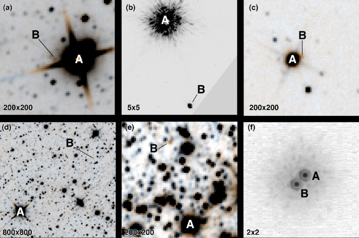
HD 13579 (0215+6740), a K2 dwarf (Bidelman 1985) at 18.6 pc (Gaia DR3): The motion object CWISER J021550.96+674017.2 from Table 2 was discovered by D. Caselden during a targeted search for companions to known 20-pc stars using multi-epoch imaging data from WISE (Figure 1a). Follow-up -band photometry from Keck/MOSFIRE (see Section A.1) shows that current location of the companion coincides with a background source, rendering the W2 = 0.780.02 mag color useless as a gauge of spectral type. The measurement of W1W2 = 0.490.02 mag from the CatWISE2020 Reject Catalog (Marocco et al. 2021) is also contaminated, as the WISE imaging sequence shown in WiseView999http://byw.tools/wiseview (Caselden et al. 2018) indicates that this is a much redder source. The motion measurement from the CatWISE2020 Reject Catalog, 39211 mas yr-1 in RA and 10210 mas yr-1 in Dec, is also contaminated by background sources but shows a magnitude and direction roughly similar to the values for the 41′′-separated K2 star HD 13579 (518.1780.012 mas yr-1 in RA and 305.6360.014 mas yr-1 in Dec; Gaia DR3). Using the WISE W2 epochal positions from the unTimely Catalog (Meisner et al. 2023a), a linear least-squares fit results in motions of 69835 mas yr-1 in RA and 50071 mas yr-1 in Dec, which are discrepant from the primary’s motion values by 5.1 and 2.7 in RA and Dec, respectively. Curiously, the CatWISE2020 and unTimely motions bracket the Gaia motion values of the primary despite the fact that both the CatWISE2020 and unTimely measurements are WISE-based and are affected by the same background contaminants. Implanting a fake source into the WiseView image sequence with the same W2 magnitude as CWISER J021550.96+674017.2 but with the Gaia-measured motions of HD 13579 provides an excellent match to observed motion of CWISER J021550.96+674017.2 itself, but suggests that the CatWISE2020 value of W2 = 13.840.01 mag may be too bright. Given the close separation between the CWISER source and HD 13579 and motions that appear similar, we tentatively denote these as a physical pair with an apparent separation of 760 AU. If associated, the distance to HD 13579 implies a spectral type of T4.5 for CWISER J021550.96+674017.2 based on the CatWISE W2 magnitude’s possibly being biased too bright.
HD 17230 (0246+1146), a K6 dwarf (Gray et al. 2003) at 16.2 pc (Gaia DR3): K. Apps (see Section 3.6.3) notes that there is a fainter star, Gaia DR3 25488745411919488 (G = 15.62 mag, = 7.51 mag), 36 south of HD 17230 that has no parallax or proper motion solution in Gaia DR3. A search of the Keck Observatory Archive101010https://koa.ipac.caltech.edu by C. Gelino reveals two epochs of observations of HD 17230 with Keck/NIRC2 behind the adaptive optics system (Wizinowich et al. 2000). Raw images in the and filters with HD 17230 under a coronagraph (PI: J. Crepp; Program ID: C182N2) clearly show a star located 3.7 from HD 17230 at a position angle of 195∘. This observation, taken on 2011 Aug 30 UT, can be compared to another taken on 2014 Oct 13 UT (PI: J. Crepp; Program ID: N100N2) in the narrow-band -continuum. Given the substantial proper motion of HD 17230 of 263.880.03 mas yr-1 in RA and mas yr-1 in Dec (Table 3.1), the fainter star should fall at a separation of and position angle of if it were a background source. However, the second epoch shows the secondary at nearly the same separation and position angle as the first epoch, proving that the two stars are a common motion pair. This conclusion is further bolstered by the 2016-epoch Gaia DR3 positions, that place the fainter star at a separation of and position angle of from HD 17230. (Figure 1b shows a first-epoch coronagraphic image in which the A component is seen only via its scattered light.) Using the Gaia DR3 parallax for the primary, this implies mag (spectral type M8) for the secondary. However, the true type might be somewhat later than this, as the lack of an astrometric solution in Gaia DR3 may mean that this companion is itself a multiple system. This companion, at an apparent physical separation of 59 AU, may be responsible for the radial velocity acceleration seen for HD 17230 over a decades-long timespan by Rosenthal et al. (2021).
G 43-23 (1002+1149), an M4 dwarf (Reid et al. 1995) at 17.9 pc (Gaia DR3): The motion object WISEU J100241.49+145914.9 from Table 2 was discovered by D. Caselden during a targeted search for companions to known 20-pc stars using multi-epoch imaging data from WISE (Figure 1c). This object lies only 156 away from G 43-23, which has astrometry from Gaia DR3 of mas, mas yr-1, and mas yr-1. WISEU J100241.49+145914.9 itself is not listed in either the CatWISE2020 Catalog or the CatWISE2020 Reject Table, but a linear least-squares fit to its epochal unTimely positions (Meisner et al. 2023a) in W2 gives motions of mas yr-1 in RA and mas yr-1 in Dec, nearly identical to the Gaia motions for the primary. Implanting a W2 = 14.55 mag source with the motions of G 43-23 into the WISE image sequence of WiseView (Caselden et al. 2018) makes for a convincing doppelgänger to WISEU J100241.49+145914.9 itself. The WISEU source’s UHS detection at mag results in a color of W2 = 3.630.11 mag, suggesting a type of T8.5 and a distance of 14.3 pc, which is slightly closer than the 17.9 pc distance measured for G 43-23. Nonetheless, given the proximity of the two objects to each other and their nearly identical motions, we consider this to be a physical pair at an apparent physical separation of 280 AU.
HD 170573 (18335415), a K4.5 dwarf (Gray et al. 2006) at 19.1 pc (Gaia DR3): The T7 dwarf CWISE J183207.94540943.3 was discovered by G. Colin and B. Pumphrey and first published in Kirkpatrick et al. (2021a), where Spitzer astrometric monitoring gave mas, mas yr-1, and mas yr-1. In assembling the full 20-pc census for this paper, it was noted that this object lies 103 from the K4.5 dwarf HD 170573 (Figure 1d), which has Gaia DR3 astrometric values of mas, mas yr-1, and mas yr-1. Until more accurate astrometry for the T dwarf becomes available, we will consider this pair to be physically associated because these values are only 1.1, 0.7, and 3.1 different for , , and , respectively. If a true binary, the projected separation is 11,800 AU.
G 155-42 (18481434), an M3 dwarf (Gaidos et al. 2014) at 17.1 pc (Gaia DR3): The motion object CWISE J184803.45143232.3 from Table 2 was discovered by S. Goodman while searching for unpublished motion objects in WISE imaging data. While assembling the 20-pc census for this paper, it was noted that this source falls 245 away from G 155-42 (Figure 1e). The CatWISE2020 Catalog (Marocco et al. 2021) lists motions for CWISE J184803.45143232.3 of mas yr-1 and mas yr-1. A linear least-squares fit to the WISE W2 epochal positions from the unTimely Catalog (Meisner et al. 2022) results in motions of mas yr-1 and mas yr-1. The Gaia DR3 astrometry for G 155-42 is mas, mas yr-1, and mas yr-1. The measured motion values between the two sources differ by 2.8 and 3.6 in RA and Dec, respectively, for the CatWISE2020 motion of the potential secondary and by 2.5 and 2.6 for the unTimely motion. The W2 color of CWISE J184803.45143232.3 from Table 2 suggests a T7.5 dwarf at a distance of 15.7 pc, which is sufficiently close to the 17.1 pc distance of G 155-42 that we tentatively consider them to be a physical pair with apparent physical separation of 2500 AU, pending improved astrometry for the secondary.
2MASS J19253089+0938235, an M8 dwarf (West et al. 2015) at 17.0 pc (Gaia DR3): C. Gelino finds two epochs of Keck/NIRC2 data for this object in the Keck Observatory Archive. The first epoch (2019 May 22 UT; PI: Bond; Program ID: H299) shows two objects separated by 194 mas at a position angle of 146∘ and magnitude difference of =0.29 mag. Two objects are still present in the second epoch (2020 Jun 2 UT; PI: Mawet; Program ID: C249) but with a separation of 199 mas and position angle of 137∘ (Figure 1f). We conclude that 2MASS J19253089+0938235 is a closely-separated binary showing orbital motion because the pair shows measurably different separations and position angles but the astrometry of the second object is inconsistent with the motion of a background star, which would have exhibited a relative motion of approximately 80 mas in RA and +240 mas in Dec. Using a UKIDSS Galactic Plane Survey DR11PLUS star visible in the field and located at J2000 RA = 291.3801844 deg and Dec= +9.6377532 deg, we find =10.530.03 mag for 2MASS J19253089+0938235A (the northwest component) and =10.820.03 mag for 2MASS J19253089+0938235B (the southeast component). This object has been flagged as a possible member of the AB Dor Moving Group (Gagné & Faherty 2018).
2.3 Checks against the Fifth Catalog of Nearby Stars
After we had completed our accounting of the 20-pc census, we were presented with an additional opportunity to further check for omissions or subtractions. Golovin et al. (2022) recently published the Fifth Catalog of Nearby Stars (CNS5), a compilation of all stars and brown dwarfs within 25 pc of the Sun. Within the CNS5, there are 3,002 objects with parallaxes of 50 mas or greater, whereas our list has 3,588 individual objects that meet this criterion111111Part of this discrepancy is due to the fact that the CNS5 has some entries whose components are not split into individual sources. Specifically, fifty entries are listed as double stars, seven as triples, and one as a quadruple. Even if these are split out as individual components, that still leaves a difference between the two lists of 519 objects.. For the purposes of checking the completeness of our own census, we find that only twenty-two of these CNS5 objects were not included in our list. These are given in Table 4. Five of these are Gaia discoveries with relatively large Gaia parallax uncertainties. We show in section A.2 that three of these are background objects based on their spectra, and we assume that the other two, given their even larger parallactic errors, are also background objects. Another fifteen have preferred parallaxes that place them beyond 20 pc, and these preferred parallaxes are either revised values in Gaia DR3 or published parallaxes (or new parallaxes discussed in Section A.3) with smaller uncertainties than those quoted in CNS5121212We consider SIPS J12561257 B to be outside of the 20-pc volume because its primary star, SIPS J12561257 A, has a smaller parallax uncertainty and falls outside 20 pc. The same is true of Ross 776, based on the parallactic measurement for Ross 826, with which it shares common proper motion. For 2MASS J13585269+3747137 and 2MASSI J2249091+320549, we suspect that the CNS5 parallax values and uncertainties come from the same source as our values, Best et al. (2020), but have been rounded; however, the CNS5 does not cite individual references for its parallax entries, so we are not able to confirm this.. The remaining two objects in Table 4 deserve special note. The first, 2MASSI J0639559741844, has a CNS5 parallax with a 16% uncertainty, so we consider our spectrophotometric distance estimate, which places the object beyond 20 pc, to be preferable. (See Kirkpatrick et al. 2021a for a discussion on the credibility of parallaxes when the uncertainties exceed 12.5%.) The second, APMPM J23304737 B, is a bit of a mystery, as we can find no corroborating evidence in the literature that it exists, and this is why it is not included in our census. In conclusion, our comparison to the CNS5 results in no new additions to our list.
| Object name | CNS5 RA Dec (J2000) | CNS5 | Our | Our reference |
|---|---|---|---|---|
| (hhmmss.ssddmmss.s) | (mas) | (mas) | ||
| (1) | (2) | (3) | (4) | (5) |
| G 39-9 | 04 22 34.31 +39 00 34.0 | 50.030.03 | 49.970.03 | Gaia DR3 |
| 2MASS J051609450445499 | 05 16 09.41 04 45 50.4 | 54.004.00 | 47.832.85 | Section 6.2 of Kirkpatrick et al. (2021a) |
| 2MASSI J0639559741844 | 06 39 55.99 74 18 44.6 | 51.008.00 | [46.1] | Table 10 of Kirkpatrick et al. (2021a) |
| WISEA J064313.95+163143.6 | 06 43 13.99 +16 31 44.0 | 50.050.27 | 49.970.25 | Gaia DR3 |
| HD 64606 AC | 07 54 33.92 01 24 45.2 | 50.740.58 | 48.550.13 | Gaia DR3 Non-single star lists |
| 2MASS J08583467+3256275 | 08 58 34.32 +32 56 26.5 | 50.303.70 | 40.93.6 | Best et al. (2020) |
| NLTT 25223 | 10 45 14.83 +49 41 26.6 | 53.130.42 | 43.310.10 | Gaia DR3 Non-single star lists |
| CD45 7872 | 12 35 58.50 45 56 14.6 | 52.673.05 | 48.210.60 | Gaia DR2 |
| SIPS J12561257 B | 12 56 01.85 12 57 24.8 | 52.003.00 | 47.270.47 | Gaia DR3 (SIPS J12561257 A) |
| Kelu-1 AB | 13 05 39.80 25 41 06.1 | 53.800.70 | 49.050.72 | Gaia DR3 |
| LP 220-13 | 13 56 40.80 +43 42 59.8 | 50.000.60 | 46.300.58 | Gaia DR3 |
| 2MASS J13585269+3747137 | 13 58 52.73 +37 47 12.8 | 50.003.00 | 49.63.1 | Best et al. (2020) |
| Gaia DR3 6305165514134625024 | 14 59 54.40 18 32 15.9 | 174.041.83 | background object | Table A2 |
| Gaia DR3 6013647666939138688 | 15 29 22.77 35 52 20.1 | 56.760.97 | background object | Table A2 |
| SDSS J163022.92+081822.0 | 16 30 22.97 +08 18 22.3 | 55.803.40 | 41.762.79 | Table A3 |
| Gaia DR3 4118195139455558016 | 17 38 53.15 20 53 56.2 | 53.162.33 | spurious parallax? | Gaia DR3 |
| Gaia DR3 4062783361232757632 | 17 59 55.76 27 38 17.1 | 59.451.18 | spurious parallax? | Gaia DR3 |
| Gaia DR3 4479498508613790464 | 18 39 31.62 +09 01 43.1 | 121.980.93 | background object | Table A2 |
| Ross 776 | 21 16 06.06 +29 51 51.5 | 50.790.46 | 49.910.02 | Gaia DR3 (Ross 826) |
| 2MASSI J2249091+320549 | 22 49 10.08 +32 05 46.3 | 50.003.00 | 49.73.2 | Best et al. (2020) |
| APMPM J23304737 B | 23 30 15.28 47 37 00.7 | 73.670.08 | — | companion doesn’t exist? |
| 2MASS J233123784718274 | 23 31 23.92 47 18 28.6 | 56.507.50 | 48.994.21 | Table A3 |
3 The 20-pc Census
Our final 20-pc census is presented in Table 3.1. The content of this table is described in more detail in the subsections that follow.
3.1 Nomenclature
Not all researchers refer to the same star by the same name, so having a list of aliases is needed. As we entered each object into the census, we searched SIMBAD for alternative names. The name listed under the heading "DefaultName" in Table 3.1 is the one that appeared as the default name in SIMBAD131313Note that SIMBAD sometimes conflates system names and individual names. For example, there is a single record combining the system Ross 614 [AB] and the individual component Ross 614 A, although the component Ross 614 B has a separate record. Correcting these associations is beyond the scope of this paper. when our initial search was performed. For all of these objects, a deep dive into the literature is required to establish the current knowledge of multiplicity, spectral type, etc., so we also list alternative names to aid the literature search. Table 3.1 therefore lists common names (e.g., Sirius), Bayer and Flamsteed designations, and designations from the HR, HD, BD, CD, and CPD catalogs. Table 3.1 also lists designations from proper motion catalogs (Wolf, Ross, L, LP, G, LHS, LFT, NLTT, LTT, LSPM, SCR, UPM, APMPM, LEHPM, WT, SIPS, PM, and PM J), white dwarf catalogs (WD, LAWD, EGGR), all-sky photometric catalogs (2MASS, WISE), all-sky astrometric catalogs (Gaia, HIC, HIP, TYC, UCAC4, TIC), along with a few other miscellaneous catalogs that also have high usage (GJ, V*, Karmn, **). The field "VarType" is filled with the type of variability seen, if the object is a known variable star; this information was taken from the General Catalog of Variable Stars141414Samus’ et al. (2017) and https://heasarc.gsfc.nasa.gov/W3Browse/all/gcvs.html. The references from which these designations were drawn are also listed in Table 3.1 and serve as an homage to the many researchers who have helped advance our knowledge of the nearby census.
A few common names ("CommonName"), not listed in SIMBAD, have been added from the list of star names151515https://www.iau.org/public/themes/naming_stars/ approved by the International Astronomical Union (IAU) and from Allen (1899), along with certain double star names from the Washington Double Star (WDS) Catalog161616http://www.astro.gsu.edu/wds/ and https://vizier.cds.unistra.fr/viz-bin/VizieR?-source=B/wds. The origin of these names is given under the heading "NamesRef", which is populated at the upper level for each system (i.e, on rows having integral values of "SystemHierarchy"). For 2MASS names, we supplemented the SIMBAD listings with the list of Gliese-2MASS crossmatches provided by Stauffer et al. (2010). For objects having no 2MASS-associated name in either of these lists, we searched the 2MASS Point Source Catalog (Cutri et al. 2003) directly. In a few cases, SIMBAD listed more than one name with the "2MASS J" prefix, and for these we also checked the 2MASS Point Source Catalog directly to remove the incorrect association.
| Column | Description | Sec | Example Entry |
|---|---|---|---|
| (1) | (2) | (3) | (4) |
| DefaultName | Default name in SIMBAD | 3.1 | nu Phe |
| #CompsOnThisRow | Number of known components for this row | 3.6.4 | 1 |
| AdoptedInitialMass | Adopted initial mass of this component () | 7 | 1.150 |
| AdoptedInitialMassErr | Uncertainty in adopted initial mass () | 7 | 0.159 |
| AdoptedInitialMassNote | Origin of adopted initial mass | 7 | TIC |
| Mass | Directly measured mass () | 4 | |
| MassErr | Uncertainty in directly measured mass () | 4 | |
| MassMethod | Method for direct mass measurement | 4 | |
| MassRef | Reference for direct mass measurement | 4 | |
| EstMassLit | Estimated mass from the literature () | 7 | |
| EstMassLitErr | Uncertainty on estimated mass from the literature () | 7 | |
| EstMassLitMethod | Method used for this estimated mass determination | 7 | |
| EstMassLitRef | Reference for this estimated mass | 7 | |
| EstMassTIC | Estimated mass from the TESS Input Catalog () | 6.3, 7 | 1.150 |
| EstMassTICErr | Uncertainty on TESS Input Catalog estimated mass () | 6.3, 7 | 0.159 |
| EstMassSH | Estimated mass from StarHorse () | 6.3, 7 | |
| EstMassSHErr | Uncertainty on StarHorse estimated mass () | 6.3, 7 | |
| EstMassMKs | Estimated mass from relation () | 6.3, 7 | |
| EstMassMKsErr | Uncertainty in relation estimated mass () | 6.3, 7 | |
| EstMassMG | Estimated mass from relation () | 6.3, 7 | |
| EstMassMGErr | Uncertainty in relation estimated mass () | 6.3, 7 | |
| Teff | Effective temperature, for L, T, Y dwarfs only (K) | 7.1 | |
| Teff_unc | Uncertainty in effective temperature (K) | 7.1 | |
| #Planets | No. of known exoplanets in NASA Exoplanet Archive | 3.6.4 | |
| RUWE | Gaia EDR3 renormalized unit weight error | 5.2 | 1.381 |
| LUWE_binary? | Possible binary flagged via local unit weight error | 5.2 | |
| Accelerator? | Accelerator flagged by Brandt (2021) or Khovritchev & Kulikova (2015) | 5.1 | |
| EstMassAt3AU | Kervella et al. (2022) mass estimate of companion if it is at 3 AU () | 5.1 | |
| EstMassAt30AU | Kervella et al. (2022) mass estimate of companion if it is at 30 AU () | 5.1 | |
| SystemHierarchy | System hierarchy value | 3.6.4 | 158 |
| #CompsInThisSystem | No. of components, if this is top level of system | 3.6.4 | 1 |
| SystemCode | System hierarchy value collapsed into an 8-digit integer | 3.6.4 | 01580000 |
| CommonName | Common name | 3.1 | |
| Bayer/Flamsteed | Bayer or Flamsteed designation | 3.1 | *nu. Phe |
| HR | Bright Star Catalogue ("Harvard Revised") designation | 3.1 | HR 370 |
| HD | Henry Draper Catalogue designation | 3.1 | HD 7570 |
| BD | Bonner Durchmusterung designation | 3.1 | |
| CD | Cordoba Durchmusterung designation | 3.1 | CD-46 346 |
| CPD | Cape Photographic Durchmusterung designation | 3.1 | CPD-46 127 |
| Wolf | Wolf motion survey designation | 3.1 | |
| Ross | Ross motion survey designation | 3.1 | |
| L | Bruce Proper Motion designation (“Luyten”, south) | 3.1 | |
| LP | Luyten Palomar designation (north) | 3.1 | |
| G | Giclas motion survey designation | 3.1 | |
| LHS | Luyten Half Second designation | 3.1 | LHS 1220 |
| LFT | Luyten Five Tenths designation | 3.1 | LFT 119 |
| NLTT | New Luyten Two Tenths | 3.1 | NLTT 4186 |
| LTT | Luyten Two Tenths designation | 3.1 | LTT 696 |
| LSPM | Lepine+Shara Proper Motion designation | 3.1 | |
| SCR | SuperCOSMOS+RECONS designation | 3.1 | |
| UPM | UCAC3 Proper Motion designation | 3.1 | |
| APMPM | Automated Plate Measurer Proper Motion designation | 3.1 | |
| LEHPM | Liverpool-Edinburgh High Proper Motion designation | 3.1 | |
| WT | Wroblewski+Torres motion survey designation | 3.1 | |
| SIPS | Southern Infrared Proper motion Survey designation | 3.1 | |
| PM | Proper Motion (B1950) survey designation | 3.1 | PM 01129-4548 |
| PM J | Proper Motion (J2000) survey designation | 3.1 | |
| WD | White Dwarf designation | 3.1 | |
| LAWD | Luyten Atlas of White Dwarfs designation | 3.1 | |
| EGGR | Eggen+Greenstein designation | 3.1 | |
| 2MASS | Two Micron All Sky Survey designation | 3.1 | 2MASS J01151112-4531540 |
| WISE | Wide-field Infrared Survey Explorer designation | 3.1 | WISE J011511.83-453152.2 |
| Gaia | Gaia designation | 3.1 | Gaia EDR3 4934923028038871296 |
| HIC | Hipparcos Input Catalogue designation | 3.1 | HIC 5862 |
| HIP | Hipparcos Catalogue designation | 3.1 | HIP 5862 |
| TYC | Tycho-2 Catalog designation | 3.1 | TYC 8033-1232-1 |
| UCAC4 | Fourth USNO CCD Astrograph Catalog designation | 3.1 | |
| TIC | TESS Input Catalog designation | 3.1 | TIC 229092427 |
| GJ | Gliese+Jahreiß nearby star catalog designation | 3.1 | GJ 55 |
| V* | Variable Star designation | 3.1 | |
| VarType | Type of variability seen, if column V* filled | 3.1 | |
| Karmn | CARMENES designation | 3.1 | |
| * | Multiple system designation | 3.1 | |
| NamesRef | Reference(s) for designations | 3.1 | SIMBAD |
| SexagesimalRA | Default J2000 right ascension, usually from SIMBAD | 3.2 | 01 15 11.1214282378 |
| SexagesimalDec | Default J2000 declination, usually from SIMBAD | 3.2 | -45 31 53.992580679 |
| RA | Decimal J2000 right ascension, if precision astrometry exists (deg) | 3.2 | 18.80055895 |
| RA_unc | Uncertainty on decimal J2000 right ascension (mas) | 3.2 | 0.0412 |
| Dec | Decimal J2000 declination, if precision astrometry exists (deg) | 3.2 | -45.53087326 |
| Dec_unc | Uncertainty on decimal J2000 declination (mas) | 3.2 | 0.0499 |
| Epoch | Epoch to which the decimal RA and Dec values above refer (yr) | 3.2 | 2016.0 |
| Parallax | Absolute parallax (mas) | 3.2 | 65.527 |
| Parallax_unc | Uncertainty in the absolute parallax (mas) | 3.2 | 0.0704 |
| PMRA | Proper motion in right ascension (mas yr-1) | 3.2 | 665.086 |
| PMRA_unc | Uncertainty in PMRA (mas yr-1) | 3.2 | 0.052 |
| PMDec | Proper motion in declination (mas yr-1) | 3.2 | 178.07 |
| PMDec_unc | Uncertainty in PMDec (mas yr-1) | 3.2 | 0.064 |
| PlxPMRef | Reference for the parallax and proper motion values | 3.2 | Gaia EDR3 |
| Constellation | Constellation in which this object falls | 3.2 | Phe |
| SpecTypeOpt | Published spectral type in the optical | 3.3 | F9 V Fe+0.4 |
| SpTOpt_indx | Machine-readable code for optical spectral type | 3.3 | 19.0 |
| SpTOpt_ref | Reference for the optical spectral type | 3.3 | Gray2006 |
| SpecTypeNIR | Published spectral type in the near-infrared | 3.3 | |
| SpTNIR_indx | Machine-readable code for the near-infrared type | 3.3 | |
| SpTNIR_ref | Reference for the near-infrared spectral type | 3.3 | |
| Gaia_RV | Radial velocity from Gaia DR3 (km s-1) | 3.5 | 11.90 |
| Gaia_RV_unc | Uncertainty in Gaia_RV (km s-1) | 3.5 | 0.12 |
| G | -band magnitude from Gaia eDR3 (mag) | 3.4 | 4.828 |
| G_unc | Uncertainty in , as provided by VizieR (mag) | 3.4 | 0.003 |
| G_BP | -band magnitude from Gaia eDR3 (mag) | 3.4 | 5.108 |
| G_BP_unc | Uncertainty in , as provided by VizieR (mag) | 3.4 | 0.003 |
| G_RP | -band magnitude from Gaia eDR3 (mag) | 3.4 | 4.380 |
| G_RP_unc | Uncertainty in , as provided by VizieR (mag) | 3.4 | 0.004 |
| JMKO | -band photometry on the MKO system (mag) | 3.4 | |
| JMKOerr | Uncertainty in JMKO (mag) | 3.4 | |
| J2MASS | -band photometry on the 2MASS system (mag) | 3.4 | 4.094 |
| J2MASSerr | Uncertainty in J2MASS (mag) | 3.4 | 0.346 |
| H | -band photometry on the MKO system (mag) | 3.4 | 3.719 |
| Herr | Uncertainty in H (mag) | 3.4 | 0.268 |
| K | -band photometry (mag) | 3.4 | |
| Kerr | Uncertainty in K (mag) | 3.4 | |
| Ks | -band photometry (mag) | 3.4 | 3.782 |
| Kserr | Uncertainty in Ks (mag) | 3.4 | 0.268 |
| JHK_ref | References for JMKO, J2MASS, H, K, and Ks | 3.4 | -22-2 |
| 2MASS_contam? | Note if the 2MASS photometry is contaminated | 3.4 | |
| W1 | W1 photometry from WISE (mag) | 3.4 | 3.714 |
| W1err | Uncertainty in W1 (mag) | 3.4 | 0.117 |
| W2 | W2 photometry from WISE (mag) | 3.4 | 3.082 |
| W2err | Uncertainty in W2 (mag) | 3.4 | 0.060 |
| W3 | W3 photometry from WISE (mag) | 3.4 | 3.689 |
| W3err | Uncertainty in W3 (mag) | 3.4 | 0.014 |
| W4 | W4 photometry from WISE (mag) | 3.4 | 3.609 |
| W4err | Uncertainty in W4 (mag) | 3.4 | 0.023 |
| WISEphot_ref | References for W1, W2, W3, and W4 | 3.4 | WWWW |
| WISE_contam? | Note if the WISE photometry is contaminated | 3.4 | |
| GeneralNotes | Special notes on this system/component |
Note. — This summary table describes the columns available in the full, online table. This table is also available at the NASA Exoplanet Archive, https://exoplanetarchive.ipac.caltech.edu/docs/20pcCensus.html.
References. — References for mass measurements and estimates, astrometry, spectral types, and general notes – Aberasturi2014=Aberasturi et al. (2014), Aberasturi2014b=Aberasturi et al. (2014b), Abt1965=Abt (1965), Abt1970=Abt (1970), Abt1976=Abt & Levy (1976), Abt1981=Abt (1981), Abt2006=Abt & Willmarth (2006), Abt2017=Abt (2017), Affer2005=Affer et al. (2005), Agati2015=Agati et al. (2015), Akeson2021=Akeson et al. (2021), Albert2011=Albert et al. (2011), Allen2000=Allen et al. (2000), Allen2012=Allen et al. (2012), AllendePrieto1999=Allende Prieto & Lambert (1999), Allers2013=Allers & Liu (2013), Alonso-Floriano2015=Alonso-Floriano et al. (2015), Andrade2019=Andrade (2019), Artigau2010=Artigau et al. (2010), Azulay2015=Azulay et al. (2015), Azulay2017=Azulay et al. (2017), Bach2009=Bach et al. (2009), Bagnulo2020=Bagnulo & Landstreet (2020), Baines2012=Baines & Armstrong (2012), Baines2018=Baines et al. (2018), Bakos2006=Bakos et al. (2006), Balega1984=Balega et al. (1984), Balega2004=Balega et al. (2004), Balega2013=Balega et al. (2013), BardalezGagliuffi2014=Bardalez Gagliuffi et al. (2014), BardalezGagliuffi2019=Bardalez Gagliuffi et al. (2019), BardalezGagliuffi2020=Bardalez Gagliuffi et al. (2020), Baroch2018=Baroch et al. (2018), Baroch2021=Baroch et al. (2021), Barry2012=Barry et al. (2012), Bartlett2017=Bartlett et al. (2017), Batten1992=Batten & Fletcher (1992), Bazot2011=Bazot et al. (2011), Bazot2018=Bazot et al. (2018), Beamin2013=Beamín et al. (2013), Beavers1985=Beavers & Salzer (1985), Beichman2011=Beichman et al. (2011), Benedict2001=Benedict et al. (2001), Benedict2016=Benedict et al. (2016), Berdnikov2008=Berdnikov & Pastukhova (2008), Bergfors2010=Bergfors et al. (2010), Bergfors2016=Bergfors et al. (2016) Bernat2010=Bernat et al. (2010) Bernkopf2012=Bernkopf et al. (2012), Berski2016=Berski & Dybczyński (2016), Best2013=Best et al. (2013), Best2015=Best et al. (2015), Best2020=Best et al. (2020), Best2021=Best et al. (2021), Beuzit2004=Beuzit et al. (2004), Bidelman1980=Bidelman (1980), Bidelman1985=Bidelman (1985), Bihain2013=Bihain et al. (2013), Biller2022=Biller et al. (2022), Bochanski2005=Bochanski et al. (2005), Bonavita2020=Bonavita & Desidera (2020), Boden1999=Boden et al. (1999), Bond2017=Bond et al. (2017), Bond2018=Bond et al. (2018), Bond2020=Bond et al. (2020), Bonfils2005=Bonfils et al. (2005), Bonfils2013=Bonfils et al. (2013), Bonnefoy2014=Bonnefoy et al. (2014), Bonnefoy2018=Bonnefoy et al. (2018), Borgniet2019=Borgniet et al. (2019), Bouy2003=Bouy et al. (2003), Bouy2004=Bouy et al. (2004), Bouy2005=Bouy et al. (2005), Bowler2015a=Bowler et al. (2015a), Bowler2015b=Bowler et al. (2015b), Bowler2019=Bowler et al. (2019), Boyajian2012=Boyajian et al. (2012), Brandao2011=Brandão et al. (2011), Brandt2014=Brandt et al. (2014), Brandt2019=Brandt et al. (2019), Brandt2020=Brandt et al. (2020), Brandt2021=Brandt (2021), BrandtG2021=Brandt et al. (2021), Breakiron1974=Breakiron & Gatewood (1974), Brewer2016=Brewer et al. (2016), Bruntt2010=Bruntt et al. (2010), Burgasser2003=Burgasser et al. (2003), Burgasser2004=Burgasser et al. (2004), Burgasser2006=Burgasser et al. (2006), Burgasser2007=Burgasser et al. (2007), Burgasser2008=Burgasser et al. (2008), Burgasser2008b=Burgasser et al. (2008b), Burgasser2010a=Burgasser et al. (2010a), Burgasser2010b=Burgasser et al. (2010b), Burgasser2011=Burgasser et al. (2011), Burgasser2013=Burgasser et al. (2013), Burgasser2015a=Burgasser et al. (2015a), Burgasser2015b=Burgasser et al. (2015b), Burningham2010=Burningham et al. (2010), Burningham2011=Burningham et al. (2011), Burningham2013=Burningham et al. (2013), Butler2017=Butler et al. (2017), Bychkov2013=Bychkov et al. (2013), Calissendorff2023=Calissendorff et al. (2023), Cannon1993=Cannon & Pickering (1993), CardonaGuillen2021=Cardona Guillén et al. (2021), Carrier2005=Carrier et al. (2005), Castro2013=Castro et al. (2013), Catalan2008b=Catalán et al. (2008b), CatWISE2020=Marocco et al. (2021), Chauvin2007=Chauvin et al. (2007), Che2011=Che et al. (2011), Chen2022=Chen et al. (2022), Chini2014=Chini et al. (2014), Chiu2006=Chiu et al. (2006), Chontos2021=Chontos et al. (2021), Christian2001=Christian et al. (2001), Christian2003=Christian et al. (2003), Cifuentes2020=Cifuentes et al. (2020), Clark2022=Clark et al. (2022), Climent2019=Climent et al. (2019), Close2007=Close et al. (2007), Compton2019=Compton et al. (2019), Corbally1984=Corbally (1984), CortesContreras2017=Cortés-Contreras et al. (2017), Cowley1967=Cowley et al. (1967), Cowley1976=Cowley (1976), Creevey2012=Creevey et al. (2012), Crifo2005=Crifo et al. (2005), Cruz2002=Cruz & Reid (2002), Cruz2003=Cruz et al. (2003), Cruz2007=Cruz et al. (2007), Cruz2009=Cruz et al. (2009), Cushing2005=Cushing et al. (2005), Cushing2011=Cushing et al. (2011), Cushing2014=Cushing et al. (2014), Cushing2016=Cushing et al. (2016), Cvetkovic2010=Cvetkovic & Ninkovic (2010), Cvetkovic2011=Cvetković et al. (2011), Dahn1988=Dahn et al. (1988), Dahn2002=Dahn et al. (2002), Dahn2017=Dahn et al. (2017), Dalba2021=Dalba et al. (2021), Damasso2020=Damasso et al. (2020), David2015=David & Hillenbrand (2015), Davison2014=Davison et al. (2014), Deacon2012a=Deacon et al. (2012a), Deacon2012b=Deacon et al. (2012b), Deacon2017=Deacon et al. (2017), Deeg2008=Deeg et al. (2008), Delfosse1999a=Delfosse et al. (1999a), Delfosse1999b=Delfosse et al. (1999b), Delrez2021=Delrez et al. (2021), Diaz2007=Díaz et al. (2007), Dieterich2012=Dieterich et al. (2012), Dieterich2014=Dieterich et al. (2014), Dieterich2018=Dieterich et al. (2018), Dieterich2021=Dieterich et al. (2021), DiFolco2004=Di Folco et al. (2004), Dittmann2014=Dittmann et al. (2014), Docobo2006=Docobo et al. (2006), Docobo2019=Docobo et al. (2019), DOrazi2017=D’Orazi et al. (2017), DosSantos2017=dos Santos et al. (2017), Downes2006=Downes et al. (2006), Ducati2011=Ducati et al. (2011), Dupuy2010=Dupuy et al. (2010), Dupuy2012=Dupuy & Liu (2012), Dupuy2016=Dupuy et al. (2016), Dupuy2017=Dupuy & Liu (2017), Dupuy2019=Dupuy et al. (2019), Duquennoy1988=Duquennoy & Mayor (1988), Duquennoy1991=Duquennoy & Mayor (1991), Durkan2018=Durkan et al. (2018), Edwards1976=Edwards (1976), Eggleton2008=Eggleton & Tokovinin (2008), Endl2006=Endl et al. (2006), Evans1961=Evans et al. (1961), Evans1964=Evans et al. (1964), Fabricius2000=Fabricius & Makarov (2000), Faherty2012=Faherty et al. (2012), Faherty2016=Faherty et al. (2016), Faherty2018=Faherty et al. (2018), Fan2000=Fan et al. (2000), Feng2021=Feng et al. (2021), Finch2016=Finch & Zacharias (2016), Finch2018=Finch et al. (2018), Fischer2014=Fischer et al. (2014), Forveille1999=Forveille et al. (1999), Forveille2004=Forveille et al. (2004), Forveille2005=Forveille et al. (2005), Fouque2018=Fouqué et al. (2018), Fuhrmann2008=Fuhrmann (2008), Fuhrmann2011=Fuhrmann et al. (2011a), Fuhrmann2012=Fuhrmann & Chini (2012a), Fuhrmann2012b=Fuhrmann et al. (2012b), Fuhrmann2016=Fuhrmann et al. (2016), Fuhrmann2017=Fuhrmann et al. (2017),
| Column | Description | Sec | Example Entry |
|---|---|---|---|
| (1) | (2) | (3) | (4) |
| …………………………… | ………………………………………………………………………………….. | ……….. | ………………………………………. |
References. — Gagne2015=Gagné et al. (2015), GaiaDR2=Gaia Collaboration et al. (2016), Gaia Collaboration et al. (2018) GaiaEDR3=Gaia Collaboration et al. (2016), Gaia Collaboration et al. (2021) GaiaDR3-NSS=Gaia Collaboration et al. (2023), Gaidos2014=Gaidos et al. (2014), Garcia2017=Garcia et al. (2017), Gardner2021=Gardner et al. (2021), Gatewood2003=Gatewood et al. (2003), Geballe2002=Geballe et al. (2002), GentileFusillo2019=Gentile Fusillo et al. (2019), Giammichele2012=Giammichele et al. (2012), Gigoyan2012=Gigoyan & Mickaelian (2012), Gizis1997=Gizis (1997), Gizis1997b=Gizis & Reid (1997b), Gizis2000=Gizis et al. (2000), Gizis2000b=Gizis et al. (2000b), Gizis2002=Gizis (2002), Gizis2002b=Gizis et al. (2002b), Gizis2011=Gizis et al. (2011), Gizis2015=Gizis et al. (2015), Gliese1991=Gliese & Jahreiß (1991), Gomes2013=Gomes et al. (2013), Goldin2006=Goldin & Makarov (2006), Goldin2007=Goldin & Makarov (2007), Goto2002=Goto et al. (2002), Grandjean2020=Grandjean et al. (2020), Gray2001=Gray et al. (2001), Gray2003=Gray et al. (2003), Gray2006=Gray et al. (2006), Greco2019=Greco et al. (2019), Griffin2004=Griffin (2004), Griffin2010=Griffin (2010), Guenther2003=Guenther & Wuchterl (2003), Guzik2016=Guzik et al. (2016), Halbwachs2000=Halbwachs et al. (2000), Halbwachs2012=Halbwachs et al. (2012), Halbwachs2018=Halbwachs et al. (2018), Hambaryan2004=Hambaryan et al. (2004), Hansen2022=Hansen (2022), Harrington1993=Harrington et al. (1993), Hartkopf1994=Hartkopf et al. (1994), Hartkopf2012=Hartkopf et al. (2012), Hatzes2012=Hatzes et al. (2012), Hawley1997=Hawley et al. (1997), Hawley2002=Hawley et al. (2002), Heintz1986=Heintz (1986), Heintz1990=Heintz (1990), Heintz1993=Heintz (1993), Heintz1994=Heintz (1994), Helminiak2009=Hełminiak et al. (2009), Helminiak2012=Hełminiak et al. (2012), Henry1994=Henry et al. (1994), Henry1999=Henry et al. (1999), Henry2002=Henry et al. (2002), Henry2004=Henry et al. (2004), Henry2006=Henry et al. (2006), Henry2018=Henry et al. (2018), HenryDraperExtension=Cannon & Pickering (1993), Herbig1977=Herbig (1977), Hinkley2011=Hinkley et al. (2011), Hipparcos=van Leeuwen (2007), Hollands2018=Hollands et al. (2018), Horch2011=Horch et al. (2011), Horch2012=Horch et al. (2012), Horch2017=Horch et al. (2017), Holberg2002=Holberg et al. (2002), Houk1982=Houk (1982), Houk1988=Houk & Smith-Moore (1988), Huber2009=Huber et al. (2009), Hussein2022=Hussein et al. (2022), Hsu2021=Hsu et al. (2021), Ireland2008=Ireland et al. (2008), Jackson1955=Jackson & Stoy (1955), Jahreiss2001=Jahreiß et al. (2001), Jahreiss2008=Jahreiß et al. (2008), Janson2012=Janson et al. (2012), Janson2014a=Janson et al. (2014a), Janson2014b=Janson et al. (2014b), Jao2003=Jao et al. (2003), Jao2008=Jao et al. (2008), Jao2011=Jao et al. (2011), Jao2014=Jao et al. (2014), Jeffers2018=Jeffers et al. (2018), Jeffers2020=Jeffers et al. (2020), Jeffries1993=Jeffries & Bromage (1993), Jodar2013=Jódar et al. (2013), Kallinger2010=Kallinger et al. (2010), Kallinger2019=Kallinger et al. (2019), Karovicova2022=Karovicova et al. (2022), Kasper2007=Kasper et al. (2007), Katoh2013=Katoh et al. (2013), Katoh2021=Katoh et al. (2021), Keenan1989=Keenan & McNeil (1989), Kellogg2015=Kellogg et al. (2015), Kendall2004=Kendall et al. (2004), Kendall2007=Kendall et al. (2007), Kennedy2012=Kennedy et al. (2012), Kervella2016=Kervella et al. (2016), Kervella2016b=Kervella et al. (2016b), Kervella2019=Kervella et al. (2019), Kervella2022=Kervella et al. (2022), Kesseli2019=Kesseli et al. (2019), Khovritchev2015=Khovritchev & Kulikova (2015), Kilic2020=Kilic et al. (2020), King2010=King et al. (2010), Kirkpatrick1991=Kirkpatrick et al. (1991), Kirkpatrick1994=Kirkpatrick & McCarthy (1994), Kirkpatrick1995=Kirkpatrick et al. (1995), Kirkpatrick1997=Kirkpatrick et al. (1997), Kirkpatrick1999=Kirkpatrick et al. (1999), Kirkpatrick2000=Kirkpatrick et al. (2000), Kirkpatrick2001=Kirkpatrick et al. (2001), Kirkpatrick2008=Kirkpatrick et al. (2008), Kirkpatrick2010=Kirkpatrick et al. (2010), Kirkpatrick2011=Kirkpatrick et al. (2011), Kirkpatrick2012=Kirkpatrick et al. (2012), Kirkpatrick2013=Kirkpatrick et al. (2013), Kirkpatrick2014=Kirkpatrick et al. (2014), Kirkpatrick2016=Kirkpatrick et al. (2016), Kirkpatrick2019=Kirkpatrick et al. (2019), Kirkpatrick2021a=Kirkpatrick et al. (2021a), Kirkpatrick2021b=Kirkpatrick et al. (2021b), Kirkpatrick2024=This paper, Kiyaeva2001=Kiyaeva et al. (2001), Kluter2018=Klüter et al. (2018), Kniazev2013=Kniazev et al. (2013), Kochukhov2009=Kochukhov et al. (2009), Kochukhov2019=Kochukhov & Shulyak (2019), Koen2017=Koen et al. (2017), Koizumi2021=Koizumi et al. (2021), Konopacky2010=Konopacky et al. (2010), Kraus2011=Kraus et al. (2011), Kuerster2008=Kürster et al. (2008), Kuzuhara2013=Kuzuhara et al. (2013), Lacour2021=Lacour et al. (2021), Lamman2020=Lamman et al. (2020), Laugier2019=Laugier et al. (2019), Law2006=Law et al. (2006), Lazorenko2018=Lazorenko & Sahlmann (2018), Lee1984=Lee (1984), Leggett2012=Leggett et al. (2012), Leinert2000=Leinert et al. (2000), Lepine2002=Lépine et al. (2002), Lepine2003=Lépine et al. (2003), Lepine2009=Lépine et al. (2009), Lepine2013=Lépine et al. (2013), Li2012=Li et al. (2012), Li2019=Li et al. (2019), Liebert2003=Liebert et al. (2003), Liebert2006=Liebert & Gizis (2006), Liebert2013=Liebert et al. (2013), Limoges2015=Limoges et al. (2015), Lindegren1997=Lindegren et al. (1997), Lindegren2018=Lindegren et al. (2018), Lindegren2021=Lindegren & Dravins (2021), Liu2002=Liu et al. (2002), Liu2005=Liu & Leggett (2005), Liu2010=Liu et al. (2010), Liu2012=Liu et al. (2012), Liu2016=Liu et al. (2016), Lloyd1994=Lloyd & Wonnacott (1994), Lodieu2005=Lodieu et al. (2005), Lodieu2007=Lodieu et al. (2007), Lodieu2012=Lodieu et al. (2012), Lodieu2022=Lodieu et al. (2022), Looper2007=Looper et al. (2007), Looper2008=Looper et al. (2008), LopezMorales2007=López-Morales (2007), Loth1998=Loth & Bidelman (1998), Loutrel2011=Loutrel et al. (2011), Low2021=Low et al. (2021), Lowrance2002=Lowrance et al. (2002), Luck2017=Luck (2017), Luhman2012=Luhman et al. (2012), Luhman2013=Luhman (2013), Luhman2014=Luhman (2014), Luhman2014b=Luhman & Sheppard (2014b), Lurie2014=Lurie et al. (2014), Mace2013a=Mace et al. (2013a), Mace2013b=Mace et al. (2013b), Mace2018=Mace et al. (2018), Makarov2007=Makarov et al. (2007), Malkov2012=Malkov et al. (2012), Malkov2006=Malkov et al. (2006), Malo2014b=Malo et al. (2014b), Malogolovets2007=Malogolovets et al. (2007), Mamajek2012=Mamajek (2012), Mamajek2018=Mamajek et al. (2018), Manjavacas2013=Manjavacas et al. (2013), Mann2019=Mann et al. (2019), Mariotti1990=Mariotti et al. (1990), Marocco2010=Marocco et al. (2010), Marocco2013=Marocco et al. (2013), Martin1995=Martin & Brandner (1995), Martin1998=Martin & Mignard (1998), Martin1998b=Martin et al. (1998b), Martin2018=Martin et al. (2018), Martinache2007=Martinache et al. (2007), Martinache2009=Martinache et al. (2009), Mason2009=Mason et al. (2009), Mason2017=Mason et al. (2017), Mason2018=Mason et al. (2018), Mason2018b=Mason et al. (2018b), McCleery2020=McCleery et al. (2020), McCook2016=McCook & Sion (2016), Meisner2020a=Meisner et al. (2020a), Meisner2020b=Meisner et al. (2020b), Mendez2021=Mendez et al. (2021), Merc2021=Merc et al. (2021), Metcalfe2021=Metcalfe et al. (2021), Mitrofanova2020=Mitrofanova et al. (2020), Mitrofanova2021=Mitrofanova et al. (2021), Monnier2007=Monnier et al. (2007), Monnier2012=Monnier et al. (2012), Montagnier2006=Montagnier et al. (2006),
| Column | Description | Sec | Example Entry |
|---|---|---|---|
| (1) | (2) | (3) | (4) |
| …………………………… | ………………………………………………………………………………….. | ……….. | ………………………………………. |
References. — Montes2006=Montes et al. (2006), Montes2007=Montes et al. (2007), Morales2009=Morales et al. (2009), Morbey1987=Morbey & Griffin (1987), Morgan1973=Morgan & Keenan (1973), Mosser2008=Mosser et al. (2008), Mugrauer2022=Mugrauer et al. (2022), Murray1986=Murray et al. (1986), Murray2011=Murray et al. (2011), Muzic2012=Mužić et al. (2012), Newton2014=Newton et al. (2014), Neuhauser2007=Neuhäuser et al. (2007), Nidever2002=Nidever et al. (2002), Nielsen2019=Nielsen et al. (2019), Nilsson2017=Nilsson et al. (2017), Nordstrom2004=Nordström et al. (2004), OBrien2023=O’Brien et al. (2023), Pan1990=Pan et al. (1990), Pepe2011=Pepe et al. (2011), Peretti2019=Peretti et al. (2019), Pettersen2006=Pettersen (2006), Phan-Bao2006=Phan-Bao & Bessell (2006), Phan-Bao2008=Phan-Bao et al. (2008), Phan-Bao2017=Phan-Bao et al. (2017), Piccotti2020=Piccotti et al. (2020), Pinamonti2022=Pinamonti et al. (2022), Pineda2016=Pineda et al. (2016), Pinfield2008=Pinfield et al. (2008), Pinfield2012=Pinfield et al. (2012), Pinfield2014a=Pinfield et al. (2014a), Pinfield2014b=Pinfield et al. (2014b), Pourbaix2000=Pourbaix (2000), Pourbaix2004=Pourbaix et al. (2004), Poveda2009=Poveda et al. (2009), Pravdo2006=Pravdo et al. (2006), Raghavan2010=Raghavan et al. (2010), Rajpurohit2013=Rajpurohit et al. (2013), Ramm2005=Ramm et al. (2005), Ramm2016=Ramm et al. (2016), Ramm2021=Ramm et al. (2021), Rebassa-Mansergas2017=Rebassa-Mansergas et al. (2017), Reffert2011=Reffert & Quirrenbach (2011), Reid1990=Reid & Mould (1990), Reid1995=Reid et al. (1995), Reid2000=Reid et al. (2000), Reid2001=Reid et al. (2001), Reid2003=Reid et al. (2003), Reid2004=Reid et al. (2004), Reid2005=Reid & Gizis (2005), Reid2006=Reid et al. (2006), Reid2007=Reid et al. (2007), Reid2008a=Reid et al. (2008a), Reid2008b=Reid et al. (2008b), Reiners2012=Reiners et al. (2012), Ren2013=Ren & Fu (2013), Reuyl1943=Reuyl (1943), Reyle2006=Reylé et al. (2006), Reyle2018=Reylé (2018), Riaz2006=Riaz et al. (2006), Ribas2003=Ribas (2003), Rice1998=Rice & Strassmeier (1998), Riedel2010=Riedel et al. (2010), Riedel2014=Riedel et al. (2014), Riedel2017=Riedel et al. (2017), Riedel2018=Riedel et al. (2018), Robert2016=Robert et al. (2016), Roberts2011=Roberts et al. (2011), Rodet2018=Rodet et al. (2018), Rodigas2011=Rodigas et al. (2011), Rodler2012=Rodler et al. (2012), Rodriguez2015=Rodriguez et al. (2015), Rosenthal2021=Rosenthal et al. (2021), Sahlmann2015=Sahlmann et al. (2015), Sahlmann2021=Sahlmann et al. (2021), Sahu2017=Sahu et al. (2017), Salama2021=Salama et al. (2021), Salama2022=Salama et al. (2022), Salim2003=Salim et al. (2003), Samus2003=Samus’ et al. (2003), Samus2017=Samus’ et al. (2017), Santos2003=Santos et al. (2003), SBC9=Pourbaix et al. (2004), SBC7=Batten et al. (1978), Schapera2022=Schapera et al. (2022), Schlieder2014=Schlieder et al. (2014), Schmidt2007=Schmidt et al. (2007), Schmidt2010=Schmidt et al. (2010), Schneider2014=Schneider et al. (2014), Schneider2015=Schneider et al. (2015), Schneider2017=Schneider et al. (2017), Schneider2019=Schneider et al. (2019), Schneider2020=Schneider et al. (2020), Schneider2021=Schneider et al. (2021), Scholz2002=Scholz & Meusinger (2002), Scholz2002b=Scholz et al. (2002b), Scholz2003=Scholz et al. (2003), Scholz2004=Scholz et al. (2004), Scholz2005=Scholz et al. (2005), Scholz2014=Scholz et al. (2014), Schuster1979=Schuster (1979), Schweitzer2019=Schweitzer et al. (2019), Segransan2000=Ségransan et al. (2000), Seifahrt2008=Seifahrt et al. (2008), Shan2017=Shan et al. (2017), Shkolnik2009=Shkolnik et al. (2009), Shkolnik2010=Shkolnik et al. (2010), Shkolnik2012=Shkolnik et al. (2012), Silverstein2022=Silverstein et al. (2022), Sion2014=Sion et al. (2014), Skemer2016=Skemer et al. (2016), Skiff2013=Skiff (2013), Skrutskie2006=Skrutskie et al. (2006), Skuljan2004=Skuljan et al. (2004), Smart-priv-comm=R. L. Smart (priv. comm.), Smart2013=Smart et al. (2013), Smart2018=Smart et al. (2018), Smith2014=Smith et al. (2014), Soderhjelm1999=Söderhjelm (1999), Soriano2010=Soriano & Vauclair (2010), Sperauskas2019=Sperauskas et al. (2019), Stassun2016=Stassun & Torres (2016), Stassun2019=Stassun et al. (2019), Stauffer2010=Stauffer et al. (2010), Stelzer2003=Stelzer & Burwitz (2003), Stepanov2020=Stepanov et al. (2020), Stephenson1967=Stephneson & Terrill (1967), Stephenson1975=Stephenson & Sanduleak (1975), Strassmeier1990=Strassmeier & Fekel (1990), Struve1954=Struve & Ratcliffe (1954), Struve1955=Struve & Franklin (1955), Subasavage2017=Subasavage et al. (2017), Takeda2007=Takeda et al. (2007), Tamazian2006=Tamazian et al. (2006), Teixeira2009=Teixeira et al. (2009), Terrien2015=Terrien et al. (2015), Thevenin2005=Thévenin et al. (2005), Thompson2013=Thompson et al. (2013), Thorstensen2003=Thorstensen & Kirkpatrick (2003), Tinney2003=Tinney et al. (2003), Tinney2014=Tinney et al. (2014), Tinney2018=Tinney et al. (2018), Tokovinin1997=Tokovinin (1997), Tokovinin2005=Tokovinin et al. (2005), Tokovinin2006=Tokovinin et al. (2006), Tokovinin2008=Tokovinin (2008), Tokovinin2012=Tokovinin et al. (2012), Tokovinin2014a=Tokovinin et al. (2014a), Tokovinin2014b=Tokovinin (2014b), Tokovinin2016=Tokovinin & Horch (2016), Tokovinin2017=Tokovinin (2017), Tokovinin2019=Tokovinin et al. (2019), Tokovinin2020=Tokovinin et al. (2020), Tokovinin2021=Tokovinin et al. (2021), Tokovinin2021b=Tokovinin (2021b), Toonen2017=Toonen et al. (2017), Torres2002=Torres & Ribas (2002), Torres2006=Torres et al. (2006), Torres2015=Torres et al. (2015), Torres2022=Torres (2022), Tremblay2020=Tremblay et al. (2020), Trifonov2020=Trifonov et al. (2020), Upgren1972=Upgren et al. (1972), Valenti2005=Valenti & Fischer (2005), vanAltena1995=van Altena et al. (1995), vanBelle2007=van Belle et al. (2007), vanBiesbroeck1974=van Biesbroeck (1974), vandeKamp1971=van de Kamp & Worth (1971), vonBraun2011=von Braun et al. (2011), Volk2003=Volk et al. (2003), Vrba2004=Vrba et al. (2004), Vrijmoet2020=Vrijmoet et al. (2020), Vrijmoet2022=Vrijmoet et al. (2022), WandDuong2015=Ward-Duong et al. (2015), WDS=http://www.astro.gsu.edu/wds/, West2008=West et al. (2008), West2011=West et al. (2011), West2015=West et al. (2015), Willmarth2016=Willmarth et al. (2016), Wilson1950=Wilson & Joy (1950), Wilson2003=Wilson, et al. (2003), Wilson2017=Wilson et al. (2017), Winters2011=Winters et al. (2011), Winters2017=Winters et al. (2017), Winters2018=Winters et al. (2018), Winters2019=Winters et al. (2019), Winters2019b=Winters et al. (2019b), Winters2020=Winters et al. (2020), Winters2021=Winters et al. (2021), Wittenmeyer2006=Wittenmyer et al. (2006), Wittenmeyer2011=Wittenmyer et al. (2011), Wittrock2017=Wittrock et al. (2017), Woitas2000=Woitas et al. (2000), Wright2013=Wright et al. (2013), Wright2018=Wright et al. (2018), Wyatt2007=Wyatt et al. (2007), Xia2019=Xia et al. (2019), Zasche2009=Zasche et al. (2009), Zeng2022=Zeng et al. (2022), Zhang2020=Zhang et al. (2020), Zhuchkov2012=Zhuchkov et al. (2012), Zurlo2018=Zurlo et al. (2018).
| Column | Description | Sec | Example Entry |
|---|---|---|---|
| (1) | (2) | (3) | (4) |
| …………………………… | ………………………………………………………………………………….. | ……….. | ………………………………………. |
Note. — Designation references: Bayer = Bayer 1603; Flamsteed = Stellarum Inerrantium Catalogus Britannicus (Flamsteed 1725) http://pbarbier.com/flamsteed/flamsteed.html, http://www.ianridpath.com/startales/flamsteed.html, Lalande 1783, Hoffleit & Jaschek 1991; HR = Schlesinger 1930, Schlesinger & Jenkins 1940, Hoffleit 1964, Hoffleit & Jaschek 1982, Hoffleit et al. 1983, Hoffleit & Jaschek 1991; HD = Cannon & Pickering 1918a, Cannon & Pickering 1918b, Cannon & Pickering 1919a, Cannon & Pickering 1919b, Cannon & Pickering 1920, Cannon & Pickering 1921, Cannon & Pickering 1922, Cannon & Pickering 1923, Cannon & Pickering 1924, Cannon 1925a, Cannon 1925b, Cannon 1927, Cannon 1928, Cannon 1931, Cannon 1936, Cannon & Mayall 1949; BD = Schönfeld 1886, Argelander 1903; CD = Thome 1890, Thome 1892, Thome 1894, Thome 1900, Thome 1914, Perrine 1932; CPD = Gill & Kapteyn 1896, Gill & Kapteyn 1897, Gill & Kapteyn 1900, Innes 1903; Wolf = Wolf 1919a, Wolf 1919b, Wolf 1919c, Wolf 1919d, Wolf 1919e, Wolf 1920a, Wolf 1920b, Wolf 1920c, Wolf 1920d, Wolf 1920e, Wolf 1920f, Wolf 1921a, Wolf 1921b, Wolf 1921c, Wolf 1921d, Wolf 1921e, Wolf 1921f, Wolf 1922, Wolf 1923a, Wolf 1923b, Wolf 1926a, Wolf 1924a, Wolf 1924b, Wolf 1924c, Wolf 1923c, Wolf 1924d, Wolf 1924e, Wolf 1924f, Wolf & Reinmuth 1925, Wolf 1925b, Wolf 1925c, Wolf 1925d, Wolf 1925e, Wolf 1925f, Wolf 1926b, Wolf 1926c, Wolf 1927a, Wolf 1927b, Wolf 1929, Wolf 1931; Ross = Ross 1925, Ross 1926a, Ross 1926b, Ross 1926c, Ross 1927, Ross 1928, Ross 1929, Ross 1930, Ross 1931, Ross 1937, Ross 1939a, Ross 1939b; L = Luyten 1963 (for which the “L” numbers were obtained from the NLTT Catalogue); LP = Luyten 1970a (specifically, volumes 1-9, 11-17, and 23-24), Luyten 1970b, Luyten 1970c, Luyten & La Bonte 1971, Luyten 1972a, Luyten 1972b, Luyten & La Bonte 1972c, Luyten 1972d, Luyten 1973a, Luyten 1973b, Luyten 1974a, Luyten 1974b, Luyten 1975a, Luyten 1975b, Luyten & Kowal 1975c, Luyten 1976a, Luyten 1976b, Luyten 1976c, Luyten 1980a, Luyten & Hughes 1980b, Luyten et al. 1981, Luyten & Hughes 1982, Luyten & Hughes 1983, Luyten et al. 1985a, Luyten et al. 1985b, Luyten & Hughes 1985c, Luyten & Hughes 1987a, Luyten & Hughes 1987b; G = Giclas et al. 1971, Giclas et al. 1978; LHS = Luyten 1979a; LFT = Luyten 1955; NLTT = Luyten 1979b, Luyten 1979c, Luyten 1980c, Luyten 1980d; LTT = Luyten 1957, Luyten 1961, Luyten 1962; LSPM = Lépine & Shara 2005, SCR = Hambly et al. 2004, Henry et al. 2004, Subasavage et al. 2005a, Subasavage et al. 2005b, Finch et al. 2007, Winters et al. 2011, Boyd et al. 2011; UPM = Finch et al. 2010, Finch et al. 2012; APMPM = Gizis et al. 1997c, Scholz et al. 1999, Schweitzer et al. 1999, Scholz et al. 2000, Reylé et al. 2002; LEHPM = Pokorny et al. 2003, Pokorny et al. 2004; WT = Wroblewski & Torres 1989, Wroblewski & Torres 1991, Wroblewski & Torres 1994, Wroblewski & Torres 1996, Wroblewski & Torres 1997, Wroblewski & Costa 1999, Wroblewski & Costa 2001; SIPS = Deacon et al. 2005, Deacon & Hambly 2007; PM = Eggen 1979, Eggen 1980; PM J = Lépine 2005b, Lépine 2008, Schlieder et al. 2010, Lépine & Gaidos 2011, Schlieder et al. 2012, Lépine et al. 2013; WD = McCook & Sion 1999; LAWD = Luyten 1949; EGGR = Eggen & Greenstein 1965a, Eggen & Greenstein 1965b, Eggen & Greenstein 1967, Greenstein 1969, Greenstein 1970, Greenstein 1974, Greenstein 1975, Greenstein 1976, Greenstein et al. 1977, Greenstein 1979, Greenstein 1980, Greenstein 1984; 2MASS = Cutri et al. 2003; WISE = Cutri et al. 2012, Cutri et al. 2013, Eisenhardt et al. 2020, Marocco et al. 2021; Gaia = Gaia Collaboration et al. 2018, Gaia Collaboration et al. 2021; HIC = Turon et al. 1993; HIP = ESA 1997, van Leeuwen 2007; TYC = Høg et al. 2000; UCAC4 = Zacharias et al. 2013; TIC = Stassun et al. 2019; GJ = Gliese 1969, Woolley et al. 1970, Gliese & Jahreiß 1979; V* = Samus et al. 2004; Karmn = Alonso-Floriano et al. 2015, Cortés-Contreras et al. 2017; ** = This designation is unique to SIMBAD (Wenger et al. 2000).
Note. — Reference for photometry is a five-character code referring to the source of the , , , , and magnitudes, respectively, with these characters as the individual codes – 2 = 2MASS (Skrutskie et al. 2006), a = Meisner et al. (2020a), A = Meisner et al. (2020b), b = Bardalez Gagliuffi et al. (2020) for which the HST F125W magnitude limit for WISE 0830+2837 is used as its value for , B = Bigelow/2MASS from Kirkpatrick et al. (2021a), c = Boccaletti et al. (2003), D = Database of Ultracool Parallaxes as of 2020 April: Dupuy & Liu (2012) and Dupuy & Kraus (2013) and Liu et al. (2016), e = Martin et al. (2018), E = McElwain & Burgasser (2006), f = Faherty et al. (2012), F = Freed et al. (2003), g = Mamajek et al. (2018), G = Gemini-South/FLAMINGOS2 from Kirkpatrick et al. (2021a), h = Pinfield et al. (2014b), H = Pinfield et al. (2014a), i = Ireland et al. (2008), I = Dupuy et al. (2019), j = Janson et al. (2011), J = Faherty et al. (2014), k = Kirkpatrick et al. (2019), K = Kirkpatrick et al. (2011), m = Mace et al. (2013a), M = Magellan/PANIC from Kirkpatrick et al. (2021a), p = PAIRITEL from Kirkpatrick et al. (2021a), P = Palomar/WIRC from Kirkpatrick et al. (2021a), Q = Deacon et al. (2017), r = Deacon et al. (2012b), s = Schneider et al. (2015), S = SOAR/OSIRIS from Kirkpatrick et al. (2021a), t = Tinney et al. (2014), T = Thompson et al. (2013), u = ULAS or UGPS or UGCS (Lawrence et al. 2007), U = UHS (Dye et al. 2018), v = VVV (Minniti et al. 2010), V = VHS (McMahon et al. 2013), w = Wright et al. (2013), W = Best et al. (2020), x = see Table 2 in this paper, z = Meisner et al. (2023b), Z = Schapera et al. (2022).
3.2 Astrometry
For each object in the 20-pc census, we list approximate sexagesimal Right Ascension (RA) and Declination (Dec) coordinates at equinox J2000, given under "SexagesimalRA" and "SexagesimalDec" in Table 3.1. For close multiple systems, the positions of the two objects may be identical, as these coordinates are meant to provide only a crude position for matching the system across catalogs. For more precise coordinates, we also provide RA and Dec in decimal degrees ("RA" and "Dec") at the yearly epoch provided in the "Epoch" column, along with the coordinate uncertainties ("RA_unc" and "Dec_unc"). Also listed are the absolute parallax ("Parallax") and its uncertainty ("Parallax_unc") and the (usually) absolute proper motions and their uncertainties in RA and Dec ("PMRA", "PMDec", "PMRA_unc", and "PMDEC_unc"). The reference for these decimal coordinates, parallax, and motion measurements is also given ("PlxPMRef"). Note that for some multiple systems, this more precise astrometry may exist only for the composite system or primary and not for each individual component. (As asterisk in the "PlxPMRef" column indicates that the parallax and motion values for another object in the system are used in lieu of actual measurements for this component.) Furthermore, for some recent brown dwarf discoveries, only positions and proper motions are given, as parallaxes have not yet been measured.
As a final note on positions, we provide the constellation in which each object is located ("Constellation"), based on the VizieR tool171717http://vizier.cfa.harvard.edu/viz-bin/VizieR?-source=VI/42 that uses the constellation boundaries provided by Roman (1987). This column can be used to determine the nearest object in each constellation, as further explored in Appendix B.
3.3 Spectral types
For higher mass stars – typically those with types earlier than mid-M – our primary sources for spectral types were the NStars papers by Gray et al. (2003) and Gray et al. (2006). This was done to assure that as many of our referenced types as possible were classified against a homogeneous system of standards, in this case, the MKK System of Morgan et al. (1943). This system was subsequently updated to the MK system of Johnson & Morgan (1953), which itself was expanded and updated by Morgan & Keenan (1973) (the revised MK system), Keenan & McNeil (1976), and Morgan et al. (1978). (See Hearnshaw 2014 more a more detailed history.)
Classification for objects of later type has followed the precepts of the MK System, thereby pushing this homogeneity into the late-M (Boeshaar 1976, Boeshaar & Tyson 1985, Kirkpatrick et al. 1991, Kirkpatrick et al. 2010), L (Kirkpatrick et al. 1999, Kirkpatrick et al. 2010), T (Burgasser et al. 2006, Kirkpatrick et al. 2010), and Y (Cushing et al. 2011, Kirkpatrick et al. 2012) dwarf sequences. Classification is dependent upon the wavelength range over which the typing is done, so Table 3.1 specifies whether the spectral type was obtained in the visible to photographic near-infrared region (1 m; "SpecTypeOpt") or the classical near-infrared region (1-2.5 m; "SpecTypeNIR"). References for the spectral types can be found under "SpTOpt_ref" and "SpTNIR_ref". For ease of plotting, the spectral types have been converted into a numerical code, with the luminosity type (if listed) ignored. The scale181818There are no O- or B-type stars within the 20-pc volume. The closest O star is Oph (O9.5 V, d = 112 pc; Howarth et al. 2014; van Leeuwen 2007), and the closest B star is Leo (B8 IVn, d = 24.3 pc; Fuhrmann et al. 2011b; van Belle & von Braun 2009; van Leeuwen 2007). is set so that 0=A0, 10=F0, 20=G0, 30=K0, 40=M0, 50=L0, 60=T0, and 70=Y0; a type of L8.5 would thus be encoded as 58.5. These codes can be found under "SpTOpt_indx" and "SpTNIR_indx". Note that the original MK classification system’s standards jump from K5 to K7 to M0 in the late-K sequence, although K6 standards were eventually added in the late 1980s (Keenan & Yorka 1988; Keenan & McNeil 1989). As a result, there are very few objects with codes of 36 or 38-39.
For white dwarfs, Table 3.1 uses types primarily taken from the compilations of Sion et al. (2014) and McCook & Sion (2016), with post-2016 discoveries taken from more recent literature or from Section A.2. The use of these references assures that all white dwarfs are on the spectroscopic classification system proposed by Liebert & Sion (1994). All white dwarf classifications have been assigned based on optical spectra, and the corresponding optical spectral index, "SpTOpt_indx", is coded to be the Liebert & Sion (1994) temperature index + 100. That is, our index is set so that DA2=102, DAZ5.8=105.8, DA9.2=109.2, DZ12.6 =112.6, etc. For any white dwarf lacking a temperature index, our spectral index has been arbitrarily assigned a code of 100, as a temperature index of 0.0 cannot exist (and no white dwarf in Table 3.1 has a temperature index lower than 2.0).
3.4 Photometry
Table 3.1 provides photometry in several systems that have hemispheric or all-sky coverage. As discussed in section 5.3, objects in the 20-pc census span a vast dynamic range in absolute luminosity, amounting to over twenty-nine magnitudes (a difference of in brightness) in -band alone. Thus, special care must be taken when choosing photometry for Table 3.1.
For the traditional "visible" wavelength regime, Gaia eDR3 magnitudes and uncertainties at , , and are listed ("G", "G_BP", "G_RP", "G_unc", "G_BP_unc", and "G_RP_unc"). The brightest reported -band magnitude is 2 mag (Gaia Collaboration et al. 2021), and objects with mag, mag, and mag have residual saturation effects, as detailed in Gaia Collaboration et al. (2021) and Riello et al. (2021). At the faint end, Gaia is complete to 20 mag (depending upon source crowding and galactic latitude; Gaia Collaboration et al. 2021), which means that the more distant late-L dwarfs in the 20-pc census, along with most of the T dwarfs and all of the Y dwarfs, are too faint for Gaia photometric measurements (figure 26 of Gaia Collaboration et al. 2020; see also figure 2 of Theissen 2018).
For the traditional near-infrared wavelength regime, , , and magnitudes are provided, with the caveat that there are two main filter systems in use: the 2MASS filter system191919https://irsa.ipac.caltech.edu/data/2MASS/docs/releases/allsky/doc/sec6_4b.html and the MKO filter system (Tokunaga et al. 2002). The -band filter is almost identical between the two, but the and filters are quite different. As a result, we provide five separate entries to cover the possibilities – , , , , and – along with their uncertainties ("JMKO", "J2MASS", "H", "K", "Ks", "JMKOerr", "J2MASSerr", "Herr", "Kerr", and "Kserr"). The references for this photometry are given in the "JHK_ref" column. The entries mostly come from 2MASS, whereas the entries come mostly from surveys based at the United Kingdom Infrared Telescope (UKIRT; e.g., the UKIRT Hemisphere Survey, UHS – McMahon et al. 2013) and the Visible and Infrared Survey Telescope for Astronomy (VISTA; e.g. the VISTA Hemisphere Survey, VHS – Dye et al. 2018). The entries come primarily from UKIRT-based surveys, whereas the entries come from both 2MASS and VISTA-based surveys. The entries are pulled from all three sets of surveys. 2MASS provides the only reliable photometry at the bright end of our sample, albeit with large uncertainties, and extends to a S/N = 10 limit of mag, mag, and mag at its faint end202020https://irsa.ipac.caltech.edu/data/2MASS/docs/releases/allsky/doc/sec2_2.html. UKIRT and VISTA provide reliable photometry between their bright limit ( mag for UHS and 11.5-12.5 mag in , , and for VHS; Dye et al. 2018, González-Fernández et al. 2018) and their detection limit ( mag for UHS and mag, mag and mag for VHS; Dye et al. 2018, González-Fernández et al. 2018) and provide higher angular resolution than 2MASS. We have therefore favored 2MASS photometry for near-infrared magnitudes brighter than 12 mag and UKIRT/VISTA for fainter magnitudes. For objects even fainter than the UKIRT/VISTA limits, or for objects in areas not yet covered by the public UKIRT and VISTA releases, we have pulled objects from the literature or from Appendix A.1.
At longer near-infrared wavelengths and extending into the near mid-infrared, we also provide WISE-based W1 (3.4 m), W2 (4.6 m), W3 (12 m), and W4 (22 m) magnitudes and their uncertainties ("W1", "W2", "W3", "W4", "W1err", "W2err", "W3err", and "W4err"). The reference for the WISE photometry is given in the "WISEphot_ref" column. For W1 and W2, magnitudes brighter than W1 8 mag and W2 7 mag were pulled from the WISE All-sky Source Catalog and fainter magnitudes were pulled from the AllWISE Source Catalog, in accordance with the suggestion made in the AllWISE Explanatory Supplement212121https://wise2.ipac.caltech.edu/docs/release/allwise/expsup/sec2_1.html. Photometry at W3 and W4 was pulled from the WISE All-sky Release. The only exceptions to the above are objects that were not detected in either of these releases and are instead found only in the CatWISE2020 Catalog. For these sources, only W1 and W2 photometry is presented, as CatWISE2020 has no W3 or W4 photometry.
In the case of 2MASS and WISE photometry, we further provide columns "2MASS_contam?" and "WISE_contam?". A "yes" in these columns indicates that the associated photometry is likely compromised by another nearby object or artifact, as judged via our by-eye assessments of the multi-epoch WiseView image blinks (Caselden et al. 2018), as the poorer image scales of 2MASS (pixel scale of 1) and WISE (pixel size of 1375) translate to a higher likelihood of source blending.
3.5 Radial velocities
3.6 Multiplicity
Even after all systems within the 20-pc volume have been noted, one difficult step remains: correctly determining, based on current knowledge, the multiplicity of each system so that each individual component can be correctly accounted for in the mass distribution. We took a multi-pronged approach at tackling this problem, as described below.
3.6.1 The "Stellar Ambassadors" program
The first approach was to crowdsource the initial reconnaissance of the literature. With the help of the citizen scientist super users of the Backyard Worlds: Planet 9 project, we set up a program whereby volunteers could sign up to investigate the multiplicity of randomly selected 20-pc systems. To make this more enjoyable, the following mission statement was provided:
"Our science-fictional Earth Coalition is currently laying the groundwork to explore all of the ‘worlds’ within 20 parsecs (65 light years) of the Sun. Scientists on the Earth Coalition’s Board of Advisors have a list of host ‘suns’ within this volume of space, but the details in that list are a bit spotty. The Coalition is seeking to flesh out these details using our Stellar Ambassadors program.
"If you choose to become a Stellar Ambassador, your role will be to represent planet Earth to a small number of stellar systems within 20 parsecs. As we reach out for the first time to each of these stellar neighbors, you will be Earth’s representative to them. But you need to be knowledgeable of the systems for which you’re responsible, and that will involve your gaining knowledge of each system you’re assigned. (By ‘system’, we’re referring to a host star and any of its companions – other stars, brown dwarfs, or exoplanets – in orbit around it.)"
Each volunteer was tasked with determining (a) the number of stars, brown dwarfs, and exoplanets in each system, (b) the spectral types of the (sub)stellar components, and (c) the masses of each component, if the masses have been measured. Each Stellar Ambassador was initially assigned a set of 12 systems, and additional sets would be assigned if the Ambassador wished to analyze more. Importantly, participants were asked to track the reference material that they used for their data collection, regardless of whether they started with SIMBAD, VizieR, Wikipedia, or some other encyclopedic compendium. In total, twenty-one super users participated in the program, which allowed us to cover 56% of the systems with primaries earlier than L0. (All 20-pc objects with primaries later than this had already been scrutinized in Kirkpatrick et al. 2021a.) These efforts were coordinated in weekly and bi-weekly calls with the volunteers.
The product of this exercise was, as expected, an inhomogeneous set of results, as individual Ambassadors concentrated on different portions of the exercise or used entirely different methodologies in their workflows. Nonetheless, it was these varied approaches that enabled us to determine the references on which it would be the most lucrative to focus our early attention. For example, despite the varied approaches, many of the same references kept appearing again and again in the Ambassadors’ reports. These repeating references underscored the vast groundwork laid by exoplanet-finding searches in characterizing potential host stars, as well as the breadth of methods used to measure masses of stars within the solar neighborhood, a topic explored more fully in Section 4. The references that arose from the Stellar Ambassador program were the first resources we used to populate Table 3.1 with information on multiplicity, mass measurements, and mass estimates.
3.6.2 In-depth literature checks
After this first reconnaissance of the oft-referenced literature, our second approach was the inevitable deep-dive into the literature for each individual object. For this, we used the extensive per-object references compiled by SIMBAD. We concentrated on literature with high-resolution imaging and radial velocity monitoring, in order to judge the multiplicity of each system. We also looked for paper titles that referenced mass measurements and variability (such as eclipsing binaries, RS CVn variables, etc.). Because of time constraints, we were not able to review each reference in detail, but a paper well stocked with results would often allow us to populate Table 3.1 with information for many systems at once, which sped up the process for objects further down the list. We also relied heavily on the Washington Double Star Catalog222222https://vizier.cds.unistra.fr/viz-bin/VizieR?-source=B/wds and the Ninth Catalog of Spectroscopic Binaries (Pourbaix et al. 2009), although the former reference lists both confirmed and possible companions that themselves must be studied individually to gauge true companionship.
3.6.3 The Apps catalog
After our in-depth literature checks were completed, we became aware of an unpublished list of objects within 30 pc of the Sun that (now co-author) K. Apps has been carefully curating since 2009. A comparison of the Apps catalog to our list revealed twenty-eight objects, mainly companions, that have been disproved via published literature but that our list still included. These have now been removed from Table 3.1. The comparison to the Apps list also revealed another twenty-three objects, almost all of which are the second components in spectroscopic binaries or companions revealed by high-resolution imaging, whose discovery literature we had missed. These objects have now been added to Table 3.1.
3.6.4 Multiplicity parameters and exoplanets
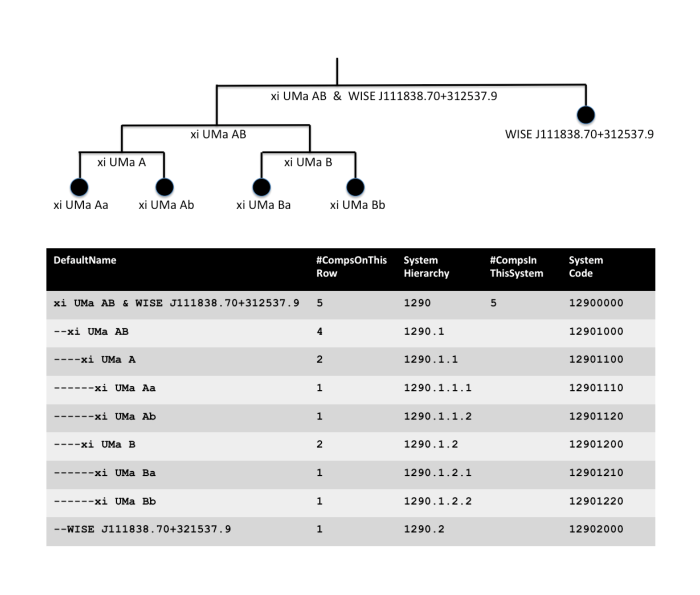
To encapsulate knowledge from the multiplicity checks above, we include several additional columns in Table 3.1 and split the components of each system into separate rows. An example for one system is illustrated in the mobile diagram (see Evans 1968) of Figure 2. In the column "DefaultName", the entry for the system as a whole appears as "xi UMa AB & WISE 111838.70+312537.9". The names of the first subdivision in the mobile diagram of this multiple are denoted by a double hyphen at the beginning of the name, which in this case are "---xi UMa AB" and "---WISE 111838.70+321537.9". Further hierarchical branches are denoted by four hyphens (e.g., "------xi UMa A"), six hyphens (e.g., "---------xi UMa Aa"), etc. The column "#CompsOnThisRow" refers to the number of known components on that row of the table. To select only individual objects in the census, for example, one can downselect only those rows for which "#CompsOnThisRow" equals 1. There is also a "SystemHierarchy" column, giving a code for each division within the system. This is comprised of a four-digit integer (e.g., "1297") that uniquely identifies the system, followed by decimal subdivisions (e.g., "1297.1" and "1297.2") to identify subcomponents. For subcomponents that are themselves binaries, further decimal subdivisions (e.g., "1297.1.1" and "1297.1.2") are assigned, etc. Table 3.1 also lists a column called "#CompsInThisSystem" that gives the total number of components in the system. This field is populated only for the top level of each system (those rows having no decimal subdivisions in the "SystemHierarchy" column) and can be summed to find the total number of individual components in the table. Additionally, Table 3.1 includes a column called "SystemCode" that collapses the "SystemHierarchy" format into an eight-digit integer comprised of the four-digit system identifier followed by four additional digits representing any other subdivisions of the "SystemHierarchy" code, but with the decimals removed (e.g., "12971210"). Note that when lower subdivisions are lacking, those digits are filled with zeroes. This "SystemCode" column is useful if the user prefers to sort the systems in Table 3.1 into their mobile diagrams rather than keeping the table’s default ordering, which sorts by RA.
Note that our accounting of components above includes only those stellar and brown dwarf members of the system, but not any of the known exoplanets. For the latter, we also include a column in Table 3.1 named "#Planets" that reports the number of exoplanets listed in the NASA Exoplanet Archive232323https://exoplanetarchive.ipac.caltech.edu/ as of 01 Sep 2022. To match objects from Table 3.1 to objects in this archive, we used the Transiting Exoplanet Survey Satellite (TESS; Ricker et al. 2015) Input Catalog (TIC; Stassun et al. 2019) designations. It should be noted that, whereas we use a formation-based definition for brown dwarfs in this paper, the NASA Exoplanet Archive uses a mass-based definition for exoplanet vs. brown dwarf and sets the dividing line, somewhat arbitrarily, at 30 MJup242424https://exoplanetarchive.ipac.caltech.edu/docs/exoplanet_criteria.html. As a result, there will be some double counting of objects, as these may appear in both the substellar and exoplanet lists. We will return to this point in Section 6.2.3.
3.7 Mass parameters and effective temperature
The final parameters in Table 3.1 relate to our need to assign masses to all individual objects within the 20-pc census. In Section 4, we discuss the various methods for which masses can be directly measured. For objects whose masses must, instead, be estimated, Section 6 provides additional discussion. Stars with measured accelerations (see Section 4.1.4) are further discussed in Section 5.1, and objects whose Gaia astrometry suggests hidden companions are discussed in Section 5.2.
Mass estimation techniques work well for hydrogen-burning stars because there is a direct mapping from color, temperature, and spectral type to mass on the main sequence. These same techniques fail for brown dwarfs because color, temperature, and spectral type vary with age, and the age of a brown dwarf is generally an unmeasurable quantity. Estimating the masses for brown dwarfs, therefore, requires a different tack, one that we approach statistically through their distribution of effective temperatures, as further discussed in Section 6.1.3.
4 Masses from Direct Measurement
There are many ways of measuring stellar masses. Some methods (1) measure mass directly using only observational data, (2) lean lightly on theoretical assumptions when a full suite of needed observational data is not available, (3) derive masses by comparing available data to an empirical data grid for stars with directly measured masses, and (4) compare observables to theoretical models. Examples of these third and fourth groups are methodologies such as The Cannon (Ness et al. 2016) and StarHorse (Queiroz et al. 2018). However, the aim of this section is to establish nearby fiducial objects for which masses have been (semi-)directly measured, in order to establish our own empirical grid (method 3) to estimate masses for the remainder of the 20-pc census. Toward this goal, we use the next two subsections to discuss methods 1 and 2 as they have been applied to nearby objects. Table 3.1 includes directly measured masses for objects that have such values ("Mass" and "Mass err") along with the technique used for the measurement ("Mass method") and its citation ("Mass reference").
4.1 Multiple systems
Mass measurements can be made for objects in binary or multiple systems, once sufficient information has been collected to define the orbits. For compact objects, mass can also be deduced from the gravitational redshift; observationally, this can only be done in multiple systems, as it requires at least one additional, non-compact, co-moving object with which to disentangle the part of the redshift due to radial velocity. More specifics are given below.
4.1.1 Visual binaries
For a visual binary whose orbit can be observed, the ratio of the masses is just
| (1) |
where and are the masses of the two objects and and are the (physical, not apparent) semi-major axes of their respective orbits. The total mass of the system, , can be derived from the equation
| (2) |
where is the gravitational constant, is the orbital period, and is the inclination of the orbit on the plane of the sky. The distance to the system must also be measured so that and are in physical, not angular, units, and the inclination can be deduced from the difference between the offset of the center of mass and the focus of the projected ellipse (Carroll & Ostlie 1996). Individual masses can be measured by combining equations 1 and 2. A list of visual (and other) multiple systems can be found in the Washington Double Star Catalog252525https://vizier.cds.unistra.fr/viz-bin/VizieR?-source=B/wds.
4.1.2 Spectroscopic binaries with eclipses
For spectroscopic binaries in which the radial velocities of both stars can be measured (SB2s), the ratio of the masses is just
| (3) |
where and are the maximum velocity amplitudes with respect to the mean radial velocity curves of the system. The sum of the masses can be obtained via the equation
| (4) |
The inclination cannot be determined unless the SB2 is also an eclipsing system, in which case the nearly edge-on orientation means that , allowing for a mass determination for both components.
There is a class of eclipsing single-lined spectroscopic binary (SB1) systems for which masses can also be derived (Stassun et al. 2017; Stevens et al. 2018). These are systems with a single stellar host and a transiting exoplanet. Because the combined light of the system is almost entirely that of the host star, available all-sky data sets can provide photometry across a wide swath of the electromagnetic spectrum – from the ultraviolet to the near mid-infrared – so that the star’s apparent bolometric luminosity can be measured. Accurate parallaxes from Gaia provide the distances needed to convert this to absolute bolometric luminosity. These photometric points span either side of the flux peak in these objects, so they also provide a semi-empirical measurement of effective temperature, as well. The radius of the host star, , can then be derived from the Stefan-Boltzmann Law
| (5) |
where is its bolometric luminosity, is its effective temperature, and is the Stefan-Boltzmann constant. In the limit where the mass and radius of the exoplanet are far smaller than those of the host star, the density of the host star, , can be calculated directly from observable quantities using the equation
| (6) |
where is the "normalized" semi-major axis (see Sandford & Kipping 2017 for details) and is the orbital period, both of which can be measured from the transit light curve. (This simplified form assumes a circular orbit. More generalized forms of this equation can be found in Seager & Mallén-Ornelas 2003.) The stellar mass, , then follows from
| (7) |
A list of SB1 and SB2 systems (see Pourbaix et al. 2009) can be found at the Centre de Données astronomiques de Strasbourg262626cdsarc.u-strasbg.fr/ftp/cats/B/sb9. A list of 158 detached eclipsing binaries with well measured stellar properties is given in Stassun & Torres (2016).
4.1.3 Astrometric binaries
Astrometric binaries are those systems in which the presence of an unseen companion can be inferred from the non-linear motion of the primary, once its parallactic motion is accounted for. A careful mapping of the astrometric orbit results in the following measurement
| (8) |
where is the mass of the luminous component, is the mass of the invisible component, is the orbital separation of the luminous component at apastron, is the eccentricity of the orbit, is the orbital period, and is the gravitational constant (Andrews et al. 2019).
It is possible to measure individual masses in astrometric binaries if the right conditions are met. We consider here an astrometric binary in which the secondary contributes little or no light to the system, as would be the case in a system comprised of a main sequence star and a black hole, neutron star, cold brown dwarf, or exoplanet companion. In this case, the light of the system comes almost entirely from the primary star, so an analysis of its broad-wavelength spectrum or spectral energy distribution built from broad-wavelength photometry can be used to deduce, with the help of empirical relations, its mass, . Then the mass of the companion, , can be measured using Equation 8. Gaia will produce orbits of hundreds of thousands of such astrometric binaries over its anticipated lifetime (Halbwachs et al. 2023).
4.1.4 Binaries with acceleration (aka proper motion anomaly)
Proper motion measurements at two different epochs have the capability of identifying hidden companions if those two motion values differ significantly from one another. (This would be labeled as an astrometric binary, see Section 4.1.3, once additional astrometric epochs are obtained.) The reason is that the proper motion of the system’s photocenter will deviate from a straight line unless both components contribute equally to the light output. This methodology was first used by Bessel (1844) to deduce hidden companions to Sirius and Procyon. An illustration of the effect, which is known both as "proper motion anomaly" and as "acceleration", is shown in Figure 3. This procedure has seen a recent revival now that high quality Hipparcos motions from the early 1990s and high quality Gaia DR2 motions from the mid-2010s can be compared.
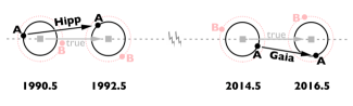
The lack of agreement between the motion measurements is sufficient to identify a hidden companion, and only a few other measurements are needed to derive the companion’s mass. This can be computed from the following equation from Brandt et al. (2019)
| (9) |
where is the projected separation between the companion and host star, is the host star’s acceleration on the plane of the sky, is the host star’s acceleration along the line of sight, and is the parallax of the system. (See Equation 17 for a different treatment.) This equation holds only if all measurements can be approximated to refer to the same orbital epoch. Otherwise, as detailed in Brandt et al. (2019), more complex orbital fitting is required.
4.1.5 Compact objects with gravitational redshifts
Finally, gravitational redshift can be used to measure the mass if the surface gravity can also be determined. Within the 20-pc sample, this is realistically measurable only in relatively massive compact objects like white dwarfs272727Brown dwarfs, like white dwarfs, are electron degenerate but are less compact and less massive, so their gravitational redshifts are only 0.5 km s-1 for the most massive examples. Although this is comparable to the effect seen for the Sun, 0.6 km s-1, it is one hundred times smaller than the effect seen for a 0.8 M⊙ white dwarf (50 km s-1).. The observed velocity shift, , due to gravitational redshift is given by
| (10) |
where is the speed of light (e.g., Chandra et al. 2020). Because the star’s mass is related to its surface gravity, , via the equation
| (11) |
the mass can be computed from
| (12) |
The surface gravity can be measured from the white dwarf’s spectrum by comparing to model atmospheres. In practice, though, this method cannot be applied to single white dwarfs because the gravitational redshift is not separable from the radial velocity. If the star is part of a co-moving multiple system or is a member of a young cluster or association, however, then the degeneracy between the radial velocity component and gravitational redshift component can be broken.
4.2 Single objects
Researchers have employed several methods that are capable of measuring the masses of individual objects. These techniques – gravitational lensing, asteroseismology, and surface convection monitoring (aka "flickering") – are described below.
4.2.1 Gravitational lensing
Gravitational lensing occurs when a mass moves very close to the line of sight between an observer and a background object. The mass of the intervening object acts as a lens that alters the apparent position of the background source as seen by the observer (Gaudi 2012) and is potentially measurable for any object. The two temporarily generated images of the background source have a morphology that is azimuthally asymmetric, and this manifests itself observationally as a shift in the centroid. The astrometric shift of the photocenter is given by
| (13) |
where is the angular Einstein radius, which can be expressed as
| (14) |
(Walker 1995, Lu et al. 2016). Here, and represent the scalar and vector time-dependent lens-source separation in the plane of the sky normalized to , is the mass of the lens, and and are the distances to the lens and source, respectively. When the distances to the lens and source are known, the monitoring of the astrometric shift as a function of time enables a measurement of the mass of the lens. These equations show that closer lenses produce larger astrometric signals, which makes this a valuable technique for measuring the masses of nearby objects, the main limitation being that such encounters of a lens and a background source happen only rarely and very accurate astrometry is needed to predict such encounters a priori. This technique has so far been successfully applied to only two objects in the 20-pc sample (Sahu et al. 2017, Zurlo et al. 2018) but promises to become more valuable as more accurate Gaia parallaxes and proper motions become available for stars all across the Milky Way.
4.2.2 Asteroseismology
Asteroseismology is the study of oscillations in stellar atmospheres, and the characteristics of these oscillations can be used to deduce a star’s physical parameters. Any star having a mechanism that can drive oscillations – such as surface convection, pulsations, tidal effects in a close binary, or opacity effects (the -mechanism) – can potentially have its mass measured. Equation 52 in Aerts (2021) can be rewritten to show that the stellar mass, , can be determined from these oscillations using the relation
| (15) |
(In the absence of a definitive theoretical model for convection, the scaling of this relation is based on observations of the Sun, as described in Kjeldsen & Bedding 1995.) Here, is the large frequency separation, is the frequency of maximum power, and is the effective temperature. The quantity can also be thought of as the inverse of twice the sound travel time between the stellar center and the stellar surface (Eq. 39 of Aerts 2021). Figures 4 and 10 of Aerts (2021) graphically demonstrate how and are measured in practice. The effective temperature, , is obtained by comparing broad-wavelength spectroscopy of the star to model atmospheres.
4.2.3 Surface convection monitoring ("flickering")
The full asteroseismology treatment above requires high-quality data over a sufficient time baseline with which to resolve the individual oscillation modes. However, variations in surface convection alone require less exquisite data and can be used to measure the mass, if certain ancillary quantities have also been well measured (Stassun et al. 2018). The needed quantity is from above, which has been shown to depend on the star’s gravity, , and effective temperature, , through the relation
| (16) |
(Brown et al. 1991), where is a normalization constant obtained by calibrating to stars with gravity measurements independently determined via asteroseismology (Kallinger et al. 2016). The effective temperature is, as above, obtained by comparing broad-wavelength spectroscopy to model atmospheres. The mass can then be measured via Equation 11, where the star’s radius can be measured directly via interferometry or through the Stefan-Boltzmann Law in Equation 5. The bolometric luminosity can be measured from the aforementioned broad-wavelength spectrum along with an accurate trigonometric parallax.
5 Multiples Lacking Sufficient Data for Mass Determination
There are some systems for which acceleration has been measured or whose astrometry indicates the presence of multiple components but for which insufficient data exist to compute the masses of the individual objects. Such systems are important to note because their mass accounting is still incomplete. This serves as an additional source of uncertainty in our mass function analysis.
5.1 Multiples known only through limited acceleration data
Currently, there are many accelerating objects within the 20-pc census that lack the additional data needed for companion mass computations via Equation 9. We nonetheless still note these as binaries in Table 3.1, and we split out those cases here for individual discussion.
Khovritchev & Kulikova (2015) have identified likely accelerators by comparing the proper motion measured between the first and second Palomar Observatory Sky Surveys (POSS-I and POSS-II; Minkowski & Abell 1963; Reid et al. 1991; Lasker & STSCI Sky-Survey Team 1998) to a motion derived using first-epoch data from other sky surveys (2MASS, SDSS, WISE) and their own second-epoch follow-up astrometry. With these two independent measurements, they can compare a long-baseline motion over 50 yr to one derived more instantaneously, over only 10 yr. Brandt (2021) have similarly intercompared the near-instantaneous Hipparcos-measured proper motion from the early 1990’s, the near-instantaneous Gaia-measured motion from the mid- to late-2010’s, and a long-baseline motion constructed from the Hipparcos-to-Gaia baseline. Both sets of authors have identified objects with significant motion discrepancies and labeled these as likely binaries. These objects are noted in Table 3.1 using the column labeled "Accelerator?".
5.1.1 Accelerators from POSS vs. recent motion comparison
The Khovritchev & Kulikova (2015) list of 2400 objects covers only a portion of the northern sky () for bright ( mag), high motion ( mas yr-1) stars. Within 20 pc of the Sun, nine such accelerators are identified, only two of which – BD+66 34 and G 96-29 (Capella HL) – were already identified as known multiples in Table 3.1. The other seven are listed in Table 9.
| J2000 RA & Dec | Name | Sp. Type |
|---|---|---|
| (1) | (2) | (3) |
| 00 38 59.04 +30 36 58.4 | Wolf 1056 | M2.5 |
| 00 57 02.69 +45 05 09.8 | G 172-30 | M3 |
| 01 03 19.84 +62 21 55.8 | Wolf 47 | M5 V |
| 01 38 21.62 +57 13 57.0 | Ross 10 | M2.5 |
| 06 01 11.05 +59 35 49.9 | G 192-13 | M3.5 V |
| 19 08 29.93 +32 16 51.6 | G 207-19 | M3.5 |
| 23 07 29.92 +68 40 05.2 | G 241-45 | M3 |
We note that none of these seven objects is identified as a high-significance accelerator in the Brandt (2021) reference discussed in the following subsection. This is because the Brandt (2021) Hipparcos-to-Gaia accelerations could not be computed for these seven stars, as none are in the Hipparcos Catalog282828Ross 10 has a Hipparcos designation in SIMBAD (HIP 7635) but does not appear in van Leeuwen (2007).. To further explore the underlying data for these Khovritchev & Kulikova (2015) accelerators, we have produced finder charts that show all seven in the POSS-I, POSS-II, 2MASS, and WISE images. A few of these appear to be blended with a background object at one of the POSS epochs. The most notably affected are G 172-30, which is blended at POSS-I with an object fainter by G = 5.8 mag; Wolf 47292929The primary in this system, BD+61 195, is 295 away from Wolf 47 itself and would not be responsible for any acceleration., which is blended at POSS-I with an object fainter by G = 6.4 mag; and G 192-13, which is blended at POSS-II with an object fainter by G = 6.2 mag. (Ross 10 moves past a star of near-equal magnitude in all of the images, the possible blending being worst at the POSS-II and 2MASS epochs.) This having been noted, whether or not objects with these magnitude differences could perturb the POSS measurements enough to affect the 50-yr proper motion measurements is not clear. Future releases from a longer baseline Gaia data set should determine whether the accelerations seen for these seven objects are real.
5.1.2 Accelerators from Hipparcos vs. Gaia comparisons
The Brandt (2021) list of 115,000 objects covers the entire sky for objects in common to Hipparcos and Gaia eDR3 ( mag). This list also gives the computed value between the two proper motions measured with the best precision, which is usually the Gaia-specific and Hipparcos-to-Gaia measurements. We conservatively set a false alarm rate of , corresponding to , to select high-confidence accelerators for analysis here. Using this criterion produces 33,750 objects, of which 194 fall within the 20-pc census. These 194 are denoted in Table 3.1 with a "yes" in the "Accelerator?" column.
Kervella et al. (2022) have also produced a catalog of possible accelerators based on a comparison of the short-baseline Gaia-specific motions and the long-baseline Hipparcos-to-Gaia motions. As this list is based on the same underlying data as the list produced by Brandt (2021), many of the same accelerators are flagged by both teams. Under the assumption that the companion mass is much less than that of the primary and that the (circular) orbit is perpendicular to the line of sight, Kervella et al. (2022) have further used the proper motion measures to estimate the mass of the hidden companion using the equation
| (17) |
where is the companion mass, is the primary mass, is the gravitational constant, is the orbital radius, (the difference in motion measurements) is in units of mas yr-1, and is in units of mas. The constant of 4740.470 is used to convert into units of m s-1 (Kervella et al. 2019). Companion masses are estimated using estimated primary masses generally from isochrone fitting for the brightest stars or from an absolute -band relation for the fainter stars, as described further in Kervella et al. (2022). Companion masses are dependent upon the unknown value of the separation between components, so Kervella et al. (2022) constructed estimates for assumed separations of 3, 5, 10, and 30 AU. In Table 3.1 we include the extrema of these mass estimates in columns labeled "EstMassAt3AU" and "EstMassAt30AU" for all objects tagged as accelerators. (In a small number of cases, a Brandt 2021 accelerator was not deemed to be an accelerator by Kervella et al. 2022, so these estimates are not given.)
| J2000 RA & Dec | Name | Sp. Type | @ 3 AU | @ 30 AU | Note | ||
|---|---|---|---|---|---|---|---|
| () | () | ||||||
| (1) | (2) | (3) | (4) | (5) | (6) | (7) | |
| 00 49 26.76 23 12 44.9 | HD 4747 AB | G9 V | 12980\@alignment@align | 0.0338 | 0.1532 | ||
| 00 50 33.25 +24 49 00.2 | FT Psc AB | M3 V keeaaSome optical spectral types for late-K and M dwarfs include information about chromospheric activity. An "e" generally indicates that H emission is present. Other values include "(k)" for slight emission reversals or infilling of the Ca II H and K lines, "k" for emission reversals in Ca II H and K that do not rise to the level of the local continuum, "ke" for such emission that rises above the local continuum level, and "kee" for strong emission in Ca II H and K along with H and possibly H and H (Gray et al. 2003). Because chromospheric activity is variable, these emission-line classification suffixes pertain only to the epoch of spectroscopic observation. | 768\@alignment@align.3 | null | null | ||
| 00 58 27.94 27 51 25.4 | CD28 302 AB | M3 V | 24\@alignment@align.25 | 0.0078 | 0.0772 | ||
| 01 41 47.13 +42 36 48.2 | HD 10307 AB | G1 V | 2540\@alignment@align | 0.1971 | 0.6338 | ||
| 01 55 57.46 51 36 32.0 | Eri AB | G9 IV | 569\@alignment@align.3 | 0.0970 | 0.1717 | ||
| 02 05 04.88 17 36 52.7 | BD18 359 AB | M3 | 6920\@alignment@align | 0.0925 | 0.6897 | ||
| 02 10 25.92 50 49 25.5 | HD 13445 AB | K1 V | 78930\@alignment@align | 0.0957 | 0.4335 | 1 known exoplanet | |
| 02 19 10.08 36 46 41.2 | L 440-30 AB | M2.5+ V | 90\@alignment@align.10 | 0.0034 | 0.0273 | ||
| 02 36 04.90 +06 53 12.4 | HD 16160 AB | K3 V | 6078\@alignment@align | 0.0942 | 0.4769 | ||
| 02 45 06.20 18 34 21.4 | Eri AB | F6 V | 4366\@alignment@align | 0.1935 | 0.5594 | ||
| 02 46 17.28 +11 46 30.9 | HD 17230 AB | K6 V | 60\@alignment@align.88 | 0.0022 | 0.0125 | ||
| 03 01 51.39 16 35 36.0 | BD17 588 ABC | M2.5 V | 215\@alignment@align.2 | 0.0147 | 0.1728 | 2 known exoplanets | |
| 03 48 01.70 +68 40 38.8 | G 221-24 AB | K6 V + M2 V | 1011\@alignment@align | 0.1764 | 1.2275 | ||
| 05 08 35.04 18 10 19.4 | L 737-9 AB | M3.5 V | 41\@alignment@align.46 | 0.0024 | 0.0169 | ||
| 05 19 12.66 03 04 25.7 | HD 34673 AB | K3 V | 2500\@alignment@align | 0.0128 | 0.0739 | ||
| 05 22 37.48 +02 36 11.6 | HD 35112 AB | K2.5 V | 192800\@alignment@align | 0.0806 | 1.0007 | ||
| 05 28 44.87 65 26 55.2 | AB Dor ACaCb | K2 V k | 1173\@alignment@align | 0.1355 | 0.6137 | ||
| 05 32 14.66 +09 49 14.9 | Ross 42 AB | M4 | 17\@alignment@align.34 | 0.0010 | 0.0079 | ||
| 05 54 22.96 +20 16 34.5 | Ori AB | G0 V CH-0.3 | 430\@alignment@align.1 | 0.0578 | 0.2097 | ||
| 06 10 34.61 21 51 52.7 | Gl 229 AB | M1 V | 13040\@alignment@align | 0.0078 | 0.0544 | 2 known exoplanets | |
| 06 17 16.13 +05 05 59.9 | HD 43587 AaAb | G0 V | 22570\@alignment@align | 0.2482 | 0.7983 | ||
| 06 26 10.25 +18 45 24.8 | HD 45088 AaAb | K3 V k | 19680\@alignment@align | 0.0712 | 0.3606 | ||
| 06 36 18.29 40 00 23.6 | CD39 2700 AB | K8 V k | 14140\@alignment@align | 0.2114 | 1.4834 | ||
| 07 16 19.77 +27 08 33.1 | G 109-55 AB | M2.5 V | 243\@alignment@align.4 | 0.0240 | 0.1787 | ||
| 07 19 31.27 +32 49 48.3 | BD+33 1505 AB | M0 V | 1301\@alignment@align | 0.0174 | 0.1160 | ||
| 07 20 07.37 +21 58 56.3 | Gem AaAb | F2 V kF0mF0 | 36\@alignment@align.94 | 0.0322 | 0.0612 | ||
| 07 28 51.36 30 14 49.3 | CD29 4446 AB | M2 | 1377\@alignment@align | 0.1433 | 0.8673 | ||
| 07 36 07.07 03 06 38.7 | BD02 2198 AB | M1 V | 18520\@alignment@align | 0.1057 | 0.7205 | ||
| 08 31 37.57 +19 23 39.4 | CU Cnc AaAbAc | M4 | 2767\@alignment@align | 0.0466 | 0.3328 | ||
| 08 36 25.47 +67 17 41.8 | BD+67 552 AB | M0.5 | 9935\@alignment@align | 0.1336 | 0.8255 | ||
| 08 39 07.90 22 39 42.8 | HD 73752 AaAbB | G5 IV | 2804\@alignment@align | 0.2452 | 0.8217 | ||
| 08 42 44.53 +09 33 24.1 | BD+10 1857 AaAb | M0 | 186\@alignment@align.0 | 0.3145 | 1.9750 | ||
| 08 57 04.68 +11 38 48.8 | BD+12 1944 AB | M1.5 | 25170\@alignment@align | 0.0973 | 0.6882 | ||
| 09 14 53.65 +04 26 34.2 | HD 79555 AB | K3+ V | 22350\@alignment@align | 0.1772 | 1.0191 | also in Table 13 | |
| 09 29 08.93 02 46 08.2 | Hya AaAb | F5.5 IV-V | 2351\@alignment@align | 0.3076 | 0.7993 | ||
| 09 32 51.43 +51 40 38.3 | UMa AB | F5.5 IV-V | 518\@alignment@align.5 | 0.0727 | 0.1540 | ||
| 09 35 39.50 +35 48 36.5 | 11 LMi AaAb | G8+ V | 496\@alignment@align.1 | 0.0091 | 0.0364 | ||
| 09 45 40.07 39 02 26.5 | L 462-119 AB | M2.5 V | 1697\@alignment@align | 0.1046 | 0.8348 | ||
| 09 53 11.78 03 41 24.4 | BD02 3000 AB | M2 | 80\@alignment@align.34 | 0.0052 | 0.0351 | ||
| 11 11 33.15 14 59 28.9 | HD 97233 AB | K5 V (k) | 471\@alignment@align.7 | 0.1108 | 0.7535 | ||
| 11 21 26.67 20 27 14.0 | HD 98712 A | K6 V ke | 6618\@alignment@align | 0.1439 | 0.8376 | ||
| 12 00 44.46 10 26 46.1 | HD 104304 AB | G8 IV | 57500\@alignment@align | 0.2325 | 0.8631 | ||
| 12 23 33.20 +67 11 18.5 | G 237-64 AB | M2.5 | 1767\@alignment@align | null | null | ||
| 12 28 57.59 +08 25 31.1 | Wolf 414 AB | M3.5 V + M5 V | 2059\@alignment@align | 0.1223 | 1.0562 | ||
| 12 44 14.55 +51 45 33.4 | HD 110833 AaAbB | K3 | 95\@alignment@align.44 | 0.0307 | 0.1438 | ||
| 13 00 46.56 +12 22 32.7 | BD+13 2618 AB | M1.5 | 3393\@alignment@align | 0.0530 | 0.3667 | 1 known exoplanet | |
| 13 19 33.59 +35 06 36.6 | BD+35 2436 AaAb | M1 | 79\@alignment@align.89 | 0.0151 | 0.0948 | ||
| 13 47 15.74 +17 27 24.8 | Boo AB | F7 IV-V | 7745\@alignment@align | 0.1133 | 0.2944 | 1 known exoplanet | |
| 13 52 35.85 50 55 18.1 | HD 120780 AaAb | K2 V | 479\@alignment@align.5 | 0.0332 | 0.1594 | ||
| 14 03 32.34 +10 47 12.3 | HD 122742 AB | G6 V | 640\@alignment@align.6 | 0.0597 | 0.2446 | ||
| 14 54 29.24 +16 06 03.8 | BD+16 2708 ABaBb | M3 V | 2764\@alignment@align | 0.0089 | 0.0654 | ||
| 15 41 16.57 +75 59 34.0 | Ross 1057 AB | M3.5 | 1780\@alignment@align | 0.0576 | 0.6208 | ||
| 15 44 01.82 +02 30 54.6 | Ser ABaBb | G5 V | 4965\@alignment@align | null | null | ||
| 16 05 40.48 20 27 00.1 | HD 144253 AB | K3 V | 189\@alignment@align.3 | 0.0439 | 0.2222 | ||
| 16 28 28.14 70 05 03.8 | TrA AaAb | F9 V | 47\@alignment@align.58 | 0.0110 | 0.0369 | ||
| 17 09 31.54 +43 40 52.8 | G 203-47 AB | M3.5 V + wd | 51\@alignment@align.01 | 0.0072 | 0.0830 | ||
| 17 19 03.84 46 38 10.4 | 41 Ara A | G9 V | 832\@alignment@align.7 | 0.0160 | 0.0689 | ||
| 17 30 11.20 51 38 13.1 | CD51 10924 AB | M0 V | 270\@alignment@align.2 | 0.0044 | 0.0274 | 4 known exoplanets | |
| 17 34 59.62 +61 52 28.2 | 26 Dra AB | G0 IV-V | 11960\@alignment@align | 0.3382 | 1.1333 | ||
| 17 46 14.42 32 06 08.4 | CD32 13298 AaAb | M3 V | 27\@alignment@align.02 | 0.0080 | 0.0597 | ||
| 17 46 27.55 +27 43 14.6 | Her AaAb | G5 IV | 12600\@alignment@align | 0.1266 | 0.4130 | ||
| 18 07 01.59 +30 33 43.6 | b Her AB | F9 V | 66470\@alignment@align | 0.0973 | 1.0649 | ||
| 18 10 26.15 62 00 08.0 | Pav AB | G0 V | 192\@alignment@align.8 | 0.0356 | 0.1192 | ||
| 18 57 01.64 +32 54 04.7 | HD 176051 AB | F9 V | 38160\@alignment@align | null | null | ||
| 19 23 34.01 +33 13 19.1 | HD 182488 AB | G9+ V | 1700\@alignment@align | 0.0085 | 0.0349 | ||
| 19 31 07.97 +58 35 09.6 | HD 184467 AB | K2 V | 27\@alignment@align.50 | 0.0314 | 0.1422 | ||
| 19 54 17.74 23 56 27.9 | HD 188088 AaAb | K2 IV (k) | 15\@alignment@align.46 | 0.0011 | 0.0050 | ||
| 20 04 06.22 +17 04 12.7 | 15 Sge AB | G0 V | 31560\@alignment@align | 0.0890 | 0.3162 | ||
| 20 05 09.78 +38 28 42.6 | HD 190771 AB | G2 V | 12760\@alignment@align | 0.0639 | 0.2319 | ||
| 20 10 19.57 20 29 36.4 | HD 191391 AB | K6 V k | 38130\@alignment@align | 0.0819 | 0.4895 | ||
| 20 44 21.95 +19 44 58.7 | HD 352860 AB | M0.5 V | 1583\@alignment@align | 0.1875 | 1.2533 | ||
| 20 56 48.54 04 50 49.1 | Ross 193 AaAb | M3 | 72\@alignment@align.54 | 0.0050 | 0.0395 | ||
| 21 00 05.39 +40 04 12.7 | BD+40 883 AaAbB | M2 | 46070\@alignment@align | 0.1350 | 0.8783 | ||
| 21 19 45.63 26 21 10.4 | HD 202940 AaAbB | G7 V | 600\@alignment@align.4 | 0.0172 | 0.1989 | ||
| 21 49 05.76 72 06 09.1 | CD72 1700 AB | M1 | 19020\@alignment@align | null | null | ||
| 22 07 00.67 +25 20 42.4 | Peg AaAb | F5 V | 66\@alignment@align.25 | 0.0205 | 0.0533 | ||
| 22 18 15.61 53 37 37.5 | HD 211415 AB | G0 V | 612\@alignment@align.3 | 0.0132 | 0.0478 | ||
| 22 36 09.69 00 50 29.8 | HD 214100 AB | M1 V | 27200\@alignment@align | 0.0672 | 0.4472 | ||
| 22 38 45.57 20 37 16.1 | FK Aqr AaAb | M2 | 47\@alignment@align.50 | 0.0014 | 0.0091 | ||
| 23 01 51.54 03 50 55.4 | HD 217580 AB | K2.5 V | 232\@alignment@align.6 | 0.0591 | 0.2966 | ||
| 23 39 20.91 +77 37 56.5 | Cep AB | K1 III | 4771\@alignment@align | 0.2376 | 0.4206 | 1 known exoplanet | |
| 23 52 25.41 +75 32 40.4 | HD 223778 AaAbB | K3 V | 124300\@alignment@align | 0.1261 | 0.5909 | ||
| 23 55 39.78 06 08 33.4 | BD06 6318 AB | M2.5 V k | 2137\@alignment@align | 0.0497 | 0.3530 | ||
| J2000 RA & Dec | Name | Sp. Type | @ 3 AU | @ 30 AU | # of | Distance to Stellar | ||
|---|---|---|---|---|---|---|---|---|
| () | () | Known Exoplanets | Companion (AU) | |||||
| (1) | (2) | (3) | (4) | (5) | (6) | (7) | (8) | |
| 00 16 12.68 79 51 04.2 | HD 1237 A | G8.5 V (k) | 26\@alignment@align.86 | 0.0019 | 0.0080 | 1 | 70 | |
| 00 18 22.88 +44 01 22.6 | GX And | M1.5 V | 2456\@alignment@align | 0.0013 | 0.0114 | 2 | 122 | |
| 03 32 55.84 09 27 29.7 | Eri | K2 V (k) | 33\@alignment@align.89 | 0.0013 | 0.0062 | 1 | ||
| 04 52 05.73 +06 28 35.6 | Wolf 1539 | M3.5 | 35\@alignment@align.10 | 0.0014 | 0.0137 | 1 | ||
| 05 11 40.59 45 01 06.4 | Kapteyn’s Star | sdM1 p | 29\@alignment@align.58 | 0.0001 | 0.0007 | 1 | ||
| 05 37 09.89 80 28 08.8 | Men | G0 V | 60\@alignment@align.98 | 0.0073 | 0.0244 | 3 | ||
| 07 54 10.88 25 18 11.4 | CD24 6144 | M0 | 18\@alignment@align.89 | 0.0007 | 0.0043 | 2 | 7110 | |
| 09 14 24.68 +52 41 10.9 | HD 79211 | K7 V | 27\@alignment@align.48 | 0.0059 | 0.0401 | 1 | 108 | |
| 10 08 43.14 +34 14 32.1 | HD 87883 | K2.5 V | 713\@alignment@align.6 | 0.0087 | 0.0408 | 1 | ||
| 16 10 24.32 +43 49 03.5 | 14 Her | K0 IV-V | 1009\@alignment@align | 0.0126 | 0.0502 | 2 | ||
| 16 12 41.78 18 52 31.8 | LP 804-27 | M3 V | 331\@alignment@align.0 | 0.0076 | 0.0562 | 1 | ||
| 20 03 37.41 +29 53 48.5 | HD 190360 | G7 IV-V | 14\@alignment@align.83 | 0.0016 | 0.0054 | 2 | 2847 | |
| 21 33 33.98 49 00 32.4 | HD 204961 | M2 | 278\@alignment@align.3 | 0.0008 | 0.0062 | 2 | ||
| 22 03 21.65 56 47 09.5 | Ind A | K4 V (k) | 287\@alignment@align.5 | 0.0030 | 0.0157 | 1 | 1464 | |
We divide the resulting list of 20-pc accelerators into three subgroups. The first, listed in Table 10, comprises eighty-three objects in known close binary and multiple systems. For all of these, the host star is known to have a close-in companion that Gaia eDR3 fails to detect or provide a full astrometric solution for, and these companions range in mass from the substellar regime into the planetary regime. For a host star at a distance of 10 pc, its Hipparcos-to-Gaia acceleration can be detected if the companion has a separation below a few100 AU (Figure 12 from Kervella et al. 2022). Companions at this separation range can also be detected with high-resolution imaging techniques or via radial velocity monitoring, and some have independently measured masses. As one example, the companion in the 19.5-yr spectroscopic binary HD 10307 AB has a measured dynamical mass from Torres (2022) of 0.2540.019 M⊙, and that system has AU, and . The Kervella et al. (2022) companion mass estimates of 0.20 M⊙ at 3 AU and 0.63 M⊙ at 30 AU bracket the dynamically measured values well, as the assumptions used were reasonable for this system. As another example, the companion to the 1.35-yr spectroscopic binary HD 184467 AB has a measured dynamical mass of 0.8680.025 M⊙ (Piccotti et al. 2020), and the system has AU, and (Arenou et al. 2000). The Kervella et al. (2022) companion mass estimate of 0.03 M⊙ at 3 AU compares unfavorably to the measured value possibly because of the Kervella et al. (2022) assumption that the secondary mass is much less than that of the primary. This demonstrates that, although the Kervella et al. (2022) companion mass estimates listed in Table 10 provide a guide as to whether the companion causing the acceleration is already known or is a still hidden member, additional astrometric data is needed before the masses can be reliably measured. As can be seen from the full entries in Table 3.1, many objects in Table 10 are triples, so it is also unclear how many objects are contributing to the measured acceleration.
The second list, shown in Table 11, gives fourteen objects known to host exoplanets but lacking any "close" stellar or substellar companions. Here we define "close" to mean within 50 AU. Six of these objects, as listed in the final column of the table, have more widely separated stellar companions at apparent separations of 70 AU. The Kervella et al. (2022) mass estimates for all fourteen of these objects are quite low and, for assumed separations of a few AU, correspond to masses traditionally thought of as being in the planetary range. Thus, the accelerations for these objects are likely caused by the known exoplanet(s) in the system. Kervella et al. (2022) provides additional analysis on the stars Eri, Kapteyn’s Star, Ind A, and Men, while noting that Kapteyn’s Star has no significant proper motion anomaly as measured by them.
The final list, shown in Table 12, has ninety-seven objects whose closest known companions are resolved by Gaia eDR3 or have no known companions at all. For many of these, the nearest known companion falls close enough to the accelerator star (100 AU; Figure 12 of Kervella et al. 2022) that it may be the object causing the acceleration. Examples are CD44 3045 A, VV Lyn Aa, CD36 6589 A, Ross 52 A, BD+45 2247 A, and Wolf 1225 A. Objects for which the nearest known companion lies beyond this separation or for which no companions are currently known are the hosts most likely to harbor new additions to the 20-pc census. Examples of stars with likely hidden companions are G 32-7, CD22 526, HD 13579, LP 837-53, HD 43162 A, HD 52698, G 250-34, BD17 3088, Vir, TrA, and Cyg.
Tables 10-12 highlight that the accounting of all components within the 20-pc census is still incomplete, as there is overwhelming evidence of additional, tightly separated companions. As only 200 of the 3,000 Gaia-detected primaries show such evidence, it is tempting to conclude that our tally of higher mass (non-exoplanet) companions is nearing completion. We caution, however, that our criteria for selecting accelerators was set very conservatively and that many real accelerators likely exist with a measured significance below our cutoff value. As the time baseline of Gaia observations is extended, accelerations will be increasingly sensitive to longer-period companions that, for higher (non-exoplanet) masses, are potentially verifiable with direct imaging techniques. Furthermore, Gaia observations over this same extended time baseline will remove the need to compare to the shallower Hipparcos data, enabling acceleration data for lower-mass primaries between the Hipparcos and Gaia limits ( mag). Finally, less than a third of all systems in the 20-pc census of Table 3.1 have both a Hipparcos entry and a Gaia DR3 astrometric solution, so many objects within our sample volume are unavailable for similar acceleration analysis.
| J2000 RA & Dec | Name | Sp. Type | @ 3 AU | @ 30 AU | # of | Dist. to Next | Note | ||
|---|---|---|---|---|---|---|---|---|---|
| () | () | Components | Nearest Known | ||||||
| in System | Member (AU) | ||||||||
| (1) | (2) | (3) | (4) | (5) | (6) | (7) | (8) | (9) | |
| 00 05 41.02 +45 48 43.6 | HD 38 A | K6 V | 6209\@alignment@align | 0.0219 | 0.1406 | 2 | 70 | ||
| 00 16 14.63 +19 51 37.5 | G 32-7 | M4 | 14\@alignment@align.42 | 0.0082 | 0.0677 | 3 | 387 | ||
| 00 45 48.29 41 54 33.1 | HD 4378 A | K5 | 64\@alignment@align.43 | 0.0021 | 0.0120 | 2 | 75 | ||
| 00 49 06.29 +57 48 54.6 | Cas A | F9 V | 659\@alignment@align.4 | 0.0220 | 0.0780 | 2 | 79 | ||
| 00 49 09.90 +05 23 19.0 | Wolf 28 | DZ7.4 | 1621\@alignment@align | 0.0007 | 0.0044 | 1 | |||
| 01 03 14.15 +20 05 52.3 | G 33-35 A | M1.5 | 28\@alignment@align.44 | 0.0040 | 0.0300 | 2 | 40 | ||
| 01 32 26.20 21 54 18.4 | CD22 526 | M1.5 V (k) | 151\@alignment@align.0 | 0.0039 | 0.0284 | 1 | |||
| 01 39 47.56 56 11 47.2 | p Eri B | K2 V | 1077\@alignment@align | 0.0184 | 0.0864 | 2 | 94 | ||
| 02 15 42.55 +67 40 20.3 | HD 13579 | K2 | 58\@alignment@align.54 | 0.0041 | 0.0184 | 2 | 736 | ||
| 02 37 52.79 58 45 11.1 | L 174-28 | M3 V | 14\@alignment@align.88 | 0.0010 | 0.0111 | 1 | |||
| 03 12 04.53 28 59 15.4 | For A | F6 V | 2451\@alignment@align | 0.0692 | 0.1861 | 3 | 75 | ||
| 03 16 13.83 +58 10 02.5 | Ross 370 A | M2 | 130\@alignment@align.2 | 0.0058 | 0.0441 | 2 | 69 | ||
| 03 23 35.26 40 04 35.0 | HD 21175 A | K1 V | 69960\@alignment@align | 0.0950 | 0.4497 | 2 | 46 | ||
| 03 48 01.03 +68 40 22.4 | HD 23189 | K2 V | 41\@alignment@align.23 | 0.0036 | 0.0222 | 3 | 303 | ||
| 03 57 28.70 01 09 34.1 | HD 24916 A | K4 V | 62\@alignment@align.16 | null | null | 3 | 168 | ||
| 04 31 11.51 +58 58 37.5 | G 175-34 | M4.5 V | 208\@alignment@align.4 | 0.0018 | 0.0203 | 2 | 57 | ||
| 04 53 31.20 55 51 37.1 | CD56 1032 A | M3 V | 117\@alignment@align.4 | 0.0032 | 0.0265 | 2 | 83 | ||
| 05 03 23.90 +53 07 42.5 | BD+52 911 A | M0.5 | 82\@alignment@align.34 | 0.0023 | 0.0167 | 2 | 78 | ||
| 05 45 48.28 +62 14 12.4 | BD+62 780 | M0 | 94\@alignment@align.82 | 0.0013 | 0.0078 | 1 | |||
| 05 55 43.21 26 51 23.4 | LP 837-53 | M2.5 V | 21\@alignment@align.48 | 0.0010 | 0.0070 | 1 | |||
| 06 13 45.30 23 51 43.0 | HD 43162 A | G6.5 V | 16\@alignment@align.04 | 0.0013 | 0.0053 | 4 | 408 | ||
| 06 33 43.28 75 37 48.0 | L 32-9 | M3 | 25\@alignment@align.61 | 0.0013 | 0.0106 | 2 | 192 | ||
| 06 37 11.23 50 02 17.7 | CD49 2340 A | K8 V (k) | 7109\@alignment@align | 0.0262 | 0.1645 | 2 | 35 | ||
| 06 57 46.63 44 17 28.2 | CD44 3045 B | M3 | 21590\@alignment@align | 0.0283 | 0.2796 | 2 | 19 | ||
| 07 01 13.73 25 56 55.5 | HD 52698 | K1 V (k) | 734\@alignment@align.1 | 0.0491 | 0.2224 | 1 | Also in Table 13 | ||
| 07 07 50.42 +67 12 04.9 | G 250-34aaA single epoch of Keck/NIRC2 data is available in the Keck Observatory Archive for this object. The - and -band observations taken on 22 Jan 2021 (UT; PI: Crepp; Program ID: D313) show an object from G 250-34 at a position angle of 328∘ and mag. No other high-resolution observations were found in other archives to help confirm or refute this possible companion. | M1.5 | 16320\@alignment@align | 0.1070 | 0.7770 | 1 | |||
| 07 31 57.71 +36 13 10.1 | VV Lyn Aa | M3 | 48470\@alignment@align | 0.0862 | 0.6179 | 3 | 19 | ||
| 07 57 57.78 00 48 51.9 | HD 65277 A | K3+ V | 645\@alignment@align.3 | 0.0081 | 0.0409 | 2 | 95 | ||
| 08 08 13.19 +21 06 18.2 | BD+21 1764 A | K7 V | 140\@alignment@align.8 | 0.0058 | 0.0359 | 4 | 190 | ||
| 08 50 42.30 +07 51 52.5 | BD+08 2131 A | K5 V | 206\@alignment@align.6 | null | null | 2 | 21 | ||
| 09 01 17.48 +15 15 56.8 | HD 77175 A | K5 | 210\@alignment@align.8 | 0.0062 | 0.0361 | 2 | 93 | ||
| 09 06 45.35 08 48 24.6 | BD08 2582 | M0 | 143\@alignment@align.1 | 0.0007 | 0.0042 | 2 | 123 | ||
| 09 14 22.77 +52 41 11.8 | HD 79210 | M0 V | 178\@alignment@align.2 | 0.0053 | 0.0344 | 2 | 108 | ||
| 09 43 55.61 +26 58 08.4 | Ross 93 | M3.5 | 23\@alignment@align.32 | 0.0023 | 0.0211 | 1 | |||
| 10 12 08.15 18 37 04.1 | BD17 3088 | M0 | 267\@alignment@align.3 | 0.0561 | 0.3563 | 2 | 7225 | ||
| 10 31 24.22 +45 31 33.8 | BD+46 1635 A | K7 V | 111\@alignment@align.8 | 0.0026 | 0.0151 | 2 | 74 | ||
| 10 41 09.30 36 53 43.7 | CD36 6589 A | M0.5 V | 101600\@alignment@align | 0.1453 | 0.9567 | 2 | 13 | ||
| 10 41 51.83 36 38 00.1 | CD35 6662 | M0 V (k) | 31\@alignment@align.36 | 0.0045 | 0.0306 | 2 | 305 | ||
| 11 05 28.58 +43 31 36.3 | BD+44 2051 A | M1 V | 25\@alignment@align.09 | 0.0004 | 0.0040 | 2 | 156 | ||
| 11 11 19.48 +43 25 02.4 | G 122-2 A | M2.5 V | 140\@alignment@align.0 | 0.0178 | 0.1259 | 2 | 60 | ||
| 11 15 11.90 +73 28 30.7 | HD 97584 A | K3 | 47\@alignment@align.01 | 0.0014 | 0.0072 | 2 | 94 | ||
| 11 34 29.49 32 49 52.8 | 20 Crt A | K0- V | 257\@alignment@align.4 | 0.0039 | 0.0175 | 2 | 146 | ||
| 11 45 34.44 20 21 12.4 | LP 793-33 | M2.5 V | 618\@alignment@align.2 | 0.0245 | 0.1946 | 2 | 295 | ||
| 11 45 42.92 64 50 29.5 | LAWD 37 | DQ6.4 | 37\@alignment@align.90 | 0.0006 | 0.0040 | 1 | |||
| 12 08 24.82 24 43 44.0 | Crv A | F1 V | 34\@alignment@align.53 | 0.0166 | 0.0431 | 2 | 47 | ||
| 12 23 00.16 +64 01 51.0 | Ross 690 | M3 | 125\@alignment@align.9 | 0.0039 | 0.0288 | 1 | |||
| 12 41 06.49 +15 22 36.0 | HD 110315 A | K4.5 V | 21830\@alignment@align | 0.0394 | 0.2098 | 2 | 32 | ||
| 12 41 39.63 01 26 57.9 | Vir A | F2 V | 551\@alignment@align.7 | 0.1854 | 0.4774 | 2 | 28 | ||
| 13 02 20.69 26 47 13.6 | HD 113194 | K5 V (k) | 82\@alignment@align.76 | 0.0092 | 0.0528 | 1 | Also in Table 13 | ||
| 13 06 15.40 +20 43 45.3 | BD+21 2486 A | K7 | 4329\@alignment@align | 0.0282 | 0.1623 | 3 | 31 | ||
| 13 14 15.14 59 06 11.7 | HD 114837 A | F6 V Fe-0.4 | 76\@alignment@align.39 | 0.0117 | 0.0327 | 2 | 84 | ||
| 13 16 51.05 +17 01 01.8 | HD 115404 A | K2.5 V (k) | 2205\@alignment@align | 0.0089 | 0.0588 | 2 | 85 | ||
| 13 20 58.05 +34 16 44.2 | BD+35 2439 | M1.5 | 199\@alignment@align.1 | 0.0042 | 0.0301 | 1 | |||
| 13 23 32.78 +29 14 15.0 | HD 116495 A | M0 V | 213\@alignment@align.5 | 0.0072 | 0.0414 | 2 | 30 | ||
| 13 28 21.08 02 21 37.1 | Ross 486 A | M3 V | 20\@alignment@align.64 | 0.0015 | 0.0118 | 2 | 112 | ||
| 13 32 44.60 +16 48 39.1 | G 63-36 A | M2.5 V | 51\@alignment@align.28 | 0.0258 | 0.1893 | 2 | 45 | ||
| 13 47 42.16 32 25 48.1 | HD 120036 A | K6.5 V (k) | 173\@alignment@align.5 | 0.0071 | 0.0431 | 2 | 135 | ||
| 13 49 04.00 +26 58 47.8 | HD 120476 A | K3.5 V | 63800\@alignment@align | 0.0441 | 0.3214 | 2 | 39 | ||
| 13 55 02.56 29 05 25.9 | HD 121271 A | M0 V k | 172300\@alignment@align | 0.0536 | 0.3033 | 2 | 38 | ||
| 14 19 00.90 25 48 55.5 | HD 125276 A | F9 V Fe-1.5 CH-0.7 | 904\@alignment@align.8 | 0.0170 | 0.0616 | 2 | 64 | ||
| 14 42 21.58 +66 03 20.8 | G 239-25 A | M2 | 62\@alignment@align.92 | 0.0056 | 0.0497 | 2 | 25 | ||
| 14 43 03.62 05 39 29.5 | Vir | F2 V | 23\@alignment@align.50 | 0.0384 | 0.0746 | 2 | 793 | ||
| 14 51 23.39 +19 06 01.6 | Boo A | G7 V | 11500\@alignment@align | 0.0689 | 0.2820 | 2 | 38 | ||
| 14 53 51.40 +23 33 21.0 | Ross 52 A | M3 V | 6509\@alignment@align | 0.1125 | 0.9852 | 2 | 10 | ||
| 14 57 28.00 21 24 55.7 | HD 131977 | K4 V | 354\@alignment@align.6 | 0.0046 | 0.0239 | 4 | 145 | ||
| 15 00 55.57 +45 25 34.6 | BD+45 2247 A | M0.5 | 80070\@alignment@align | 0.0951 | 0.6269 | 2 | 23 | ||
| 15 47 29.10 37 54 58.7 | HD 140901 A | G7 IV-V | 18\@alignment@align.43 | 0.0023 | 0.0085 | 2 | 220 | ||
| 15 55 08.56 63 25 50.6 | TrA | F1 V | 31\@alignment@align.48 | 0.0163 | 0.0295 | 1 | |||
| 16 16 45.31 +67 15 22.5 | EW Dra | M3 | 15\@alignment@align.22 | 0.0007 | 0.0052 | 2 | 695 | ||
| 16 20 03.51 37 31 44.4 | CD37 10765 A | M2 V | 2809\@alignment@align | 0.0074 | 0.0656 | 2 | 36 | ||
| 16 28 52.66 +18 24 50.6 | HD 148653 A | K2 V | 2069\@alignment@align | 0.0163 | 0.0827 | 2 | 46 | ||
| 16 55 25.22 08 19 21.3 | Wolf 629 | M3.5 V | 15\@alignment@align.84 | 0.0005 | 0.0059 | 5 | 469 | ||
| 16 55 38.01 32 04 03.7 | HD 152606 | K8 V k | 1687\@alignment@align | 0.0142 | 0.0874 | 1 | |||
| 16 56 48.57 39 05 38.2 | CD38 11343 A | M3 | 550\@alignment@align.3 | 0.0184 | 0.1312 | 3 | 49 | ||
| 16 57 53.18 +47 22 00.1 | HD 153557 A | K3 V | 875\@alignment@align.6 | 0.0102 | 0.0514 | 3 | 91 | ||
| 17 15 20.98 26 36 10.2 | 36 Oph B | K0 V | 29\@alignment@align.24 | 0.0017 | 0.0078 | 3 | 30 | ||
| 17 21 00.37 21 06 46.6 | Oph A | F2 V | 82\@alignment@align.92 | 0.0248 | 0.0646 | 2 | 71 | ||
| 17 35 13.62 48 40 51.1 | CD48 11837 A | M1.5 V | 8601\@alignment@align | 0.0174 | 0.1332 | 2 | 45 | ||
| 17 46 34.23 57 19 08.6 | L 205-128 | M4 | 37\@alignment@align.12 | 0.0001 | 0.0012 | 1 | |||
| 17 57 48.50 +04 41 36.1 | Barnard’s Star | M4 V | 74\@alignment@align.89 | 0.0000 | 0.0005 | 1 | |||
| 18 42 46.70 +59 37 49.4 | HD 173739 | M3 V | 723\@alignment@align.0 | 0.0020 | 0.0209 | 2 | 41 | ||
| 18 42 46.89 +59 37 36.7 | HD 173740 | M3.5 V | 91\@alignment@align.38 | 0.0026 | 0.0309 | 2 | 41 | ||
| 18 57 30.59 55 59 30.8 | HD 175224 A | M1 | 412\@alignment@align.4 | 0.0066 | 0.0378 | 2 | 33 | ||
| 19 36 26.53 +50 13 16.0 | Cyg | F3+ V | 103\@alignment@align.1 | 0.0277 | 0.0648 | 2 | 2150 | Other component in Table 13 | |
| 19 45 49.75 +32 23 13.7 | G 125-30 | M1.5 | 25\@alignment@align.44 | 0.0044 | 0.0353 | 1 | |||
| 19 46 23.93 +32 01 01.4 | HD 331161 A | M0.5 V | 420\@alignment@align.0 | 0.0068 | 0.0472 | 2 | 79 | ||
| 20 02 34.16 +15 35 31.5 | HD 190067 A | K0 V Fe-0.9 | 679\@alignment@align.7 | 0.0071 | 0.0322 | 2 | 62 | ||
| 20 41 51.13 32 26 06.7 | AT Mic A | M4.5 V | 20360\@alignment@align | 0.0891 | 0.5735 | 3 | 21 | ||
| 21 02 40.75 +45 53 05.2 | HD 200560 A | K2.5 V | 6003\@alignment@align | 0.0230 | 0.1106 | 2 | 52 | ||
| 21 06 53.94 +38 44 57.9 | 61 Cyg A | K5 V | 317\@alignment@align.4 | 0.0068 | 0.0386 | 2 | 111 | ||
| 21 06 55.26 +38 44 31.4 | 61 Cyg B | K7 V | 16640\@alignment@align | 0.0070 | 0.0431 | 2 | 111 | ||
| 21 07 10.38 13 55 22.5 | HD 200968 A | G9.5 V (k) | 4553\@alignment@align | 0.0180 | 0.0816 | 2 | 64 | ||
| 21 38 00.39 +27 43 25.4 | BD+27 4120 A | M0.5+ V | 359\@alignment@align.2 | 0.0266 | 0.1860 | 2 | 44 | ||
| 22 14 31.41 +27 51 18.7 | G 188-49 A | K7.5 | 20\@alignment@align.55 | 0.0023 | 0.0157 | 2 | 59 | ||
| 22 23 29.13 +32 27 33.9 | Wolf 1225 A | M3.5 | 5174\@alignment@align | 0.1158 | 0.7867 | 2 | 19 | ||
| 23 31 52.17 +19 56 14.1 | BD+19 5116 A | M3.5 V | 17570\@alignment@align | 0.0172 | 0.1549 | 2 | 34 | ||
| 23 39 37.39 72 43 19.8 | HD 222237 | K3+ V | 700\@alignment@align.6 | 0.0046 | 0.0231 | 1 | |||
5.2 Multiples with large RUWE values
The Gaia Renormalized Unit Weight Error (RUWE) is a measure of the goodness of fit of the single-star astrometric model to the observed astrometry and is expected to be 1.0 if the fit is a good representation (Lindegren et al. 2021b). This parameter is pulled from Gaia DR3 and is listed in the "RUWE" column of Table 3.1. Values significantly higher than unity can indicate either that the object is an unresolved, physical multiple (Penoyre et al. 2020) or that some other effect is causing the photocenter to deviate from expectations. Two examples of the latter are a chance alignment with a marginally resolved background star or single-star variability that confounds the RUWE renormalization itself (Belokurov et al. 2020). The typically quoted value for selecting likely binaries using this statistic is RUWE 1.4 (e.g., Fabricius et al. 2021), although Stassun & Torres (2021) have shown that values of 1.0 RUWE 1.4 are also highly predictive of unresolved multiplicity. While the RUWE normalization works well across the full population of Gaia-measured stars, Penoyre et al. (2022b) note that it does a somewhat less adequate job when a selection of nearby (d 100 pc; the GCNS of Gaia Collaboration et al. 2020) stars alone is analyzed. For that reason, they define a new statistic, which they term the Local Unit Weighted Error (LUWE), that improves upon RUWE for these nearer objects.
Values of RUWE and LUWE change with each subsequent release of Gaia data, and there is valuable information contained within the differences. Later Gaia releases have data (and astrometric solutions) covering a longer timespan, so for unresolved multiple systems with periods roughly equal to or longer than the timespans of the data release, the RUWE (or LUWE) values may continue to run high or even become larger between Gaia DR2 and Gaia eDR3 simply because the photocentric displacement caused by orbital motion in an unresolved binary makes the single-object astrometric solution fit less well with an extended data set. (See Penoyre et al. 2022a for additional discussion.) Conversely, unresolved binaries with shorter periods should improve and eventually get full astrometric solutions in the Gaia non-single star lists.
With these observations in mind, Penoyre et al. (2022b) devised a two-part criterion to select the most likely hidden multiples in the 100-pc sample: (1) LUWE and (2) . Within our 20-pc census, 104 objects meet these criteria, and these are the ones labeled with a "yes" in the Table 3.1 column named "LUWE_binary?". Of these, 73 are known from previous literature to be binary and were already labeled as such in our census. The other 31, listed in Table 13, are newly identified multiples. Nine of these are part of higher-order multiples, as indicated by the notes in the table. For eight of these systems, Gaia has detections of both the new high-LUWE object and the other component (sometimes a double itself) with which it has physical companionship. The ninth system, however, is a new triple system for which Gaia detects only the new high-LUWE binary G 43-23 but not the common-proper-motion T dwarf companion, WISEU J100241.49+145914.9, discussed in Section 2.2. Note that the LUWE criteria from Penoyre et al. (2022b) are meant to be conservative, so other hidden binaries will exist with LUWE or LUWE values outside of the bounds noted above.
| J2000 RA | J2000 Dec | Name | Note | Sp. TypeaaSpectral types are taken from Table 3.1. All are optical types except for LP 440-17, which is a near-infrared type. |
|---|---|---|---|---|
| (1) | (2) | (3) | (4) | (5) |
| 01 46 29.35 | 53 39 32.6 | 2MASS J014629355339325 | 1 | M4.5e |
| 04 34 45.33 | 00 26 46.5 | G 82-33 | M4 V | |
| 07 01 13.73 | 25 56 55.5 | HD 52698bbThis object is also in the accelerator list of Table 12. | K1 V (k) | |
| 07 08 07.01 | 22 48 47.3 | LP 840-16 | M2 | |
| 07 49 42.14 | 03 20 34.0 | UCAC4 434-042012 | 2 | M3.5 V |
| 08 25 52.82 | +69 02 01.1 | LP 35-347 | M5.5 V | |
| 10 02 42.45 | +14 59 13.0 | G 43-23 | 3 | M4 V |
| 10 14 53.12 | +21 23 46.0 | G 54-19 | M4.5 V | |
| 10 39 45.41 | 44 30 37.0 | TYC 7722-1583-1 | M3 | |
| 11 45 34.44 | 20 21 12.4 | LP 793-33 | 4 | M2.5 V |
| 13 02 20.69 | 26 47 13.6 | HD 113194bbThis object is also in the accelerator list of Table 12. | K5 V (k) | |
| 13 30 40.95 | 20 39 03.7 | UCAC4 347-066233 | M4 | |
| 13 40 08.79 | +43 46 38.0 | Ross 1026 | M3.5 | |
| 13 58 52.21 | +27 52 14.2 | UPM J1358+2752 | ||
| 14 17 22.10 | +45 25 46.0 | FBS 1415+456 | 5 | M5/6 |
| 14 23 43.74 | +14 26 51.4 | LP 440-17 | M7 (NIR) | |
| 14 24 18.70 | 35 14 32.7 | 2MASSI J1424187351432 | M6.5 V | |
| 14 28 17.58 | +05 18 45.8 | G 65-53 | 6 | M3.5 |
| 15 10 16.82 | 02 41 08.1 | TVLM 868-110639 | M9 V | |
| 15 18 31.46 | +20 36 28.2 | UCAC4 554-051865 | M4.5 V | |
| 15 52 06.55 | 33 59 19.0 | UCAC3 113-186615 | ||
| 17 33 53.18 | +16 55 13.1 | LSPM J1733+1655 | M5.5 | |
| 18 30 39.45 | 03 56 18.9 | UCAC4 431-076686 | M4.5 V | |
| 18 43 12.51 | 33 22 46.1 | CD33 13497 | 7 | M1 |
| 18 53 25.37 | +02 50 48.7 | G 141-46 | M2.5 | |
| 19 36 14.39 | +50 13 10.1 | UCAC3 281-150921 | 8 | M2/3 |
| 20 12 59.94 | +01 12 58.3 | 2MASS J20125995+0112584 | M6 | |
| 20 33 36.67 | 21 20 10.1 | 2MASS J203336682120096 | M2 | |
| 22 10 13.19 | 71 46 06.2 | PM J221027146 | ||
| 22 17 18.97 | 08 48 12.3 | Wolf 1561 A | 9 | M4 V |
| 22 24 24.65 | 58 26 13.6 | UCAC3 64-480761 |
Note. —
-
•
(1) 01465339: This is the 359-distant companion to the F9 dwarf q01 Eri.
-
•
(2) 07490320: This is the 39-distant companion to the M3.5 binary PM J074980317 AB.
-
•
(3) 1002+1459: This object also has a 156-distant companion, WISEU J100241.49+145914.9, announced in this paper (Section 2.2).
-
•
(4) 11452021: This is a physical system with the M5e star LP 793-34, 152 distant.
-
•
(5) 1417+4525: This is the 592-distant companion of the M0 star BD+46 1951.
-
•
(6) 1428+0518: This is a physical system with the M4 star G 65-54, 10 distant.
-
•
(7) 18433322: This is a physical system with the M6 star CE 507, 150 distant.
-
•
(8) 1936+5013: This is the 19-distant companion to the F3+ dwarf Cyg, which is listed amongst the accelerators in Table 12.
-
•
(9) 22170848: This is a physical system with the M5 dwarf binary Wolf 1561 BaBb, 79 distant.
5.3 Multiplicity (and oddities) identified through color-magnitude diagrams
In Figures 4-9, we show several color-type, color-color, and color-magnitude diagrams as a final method for identifying unresolved binaries. These diagrams also illustrate the rich diversity of colors and absolute magnitudes that objects within the 20-pc census possess.
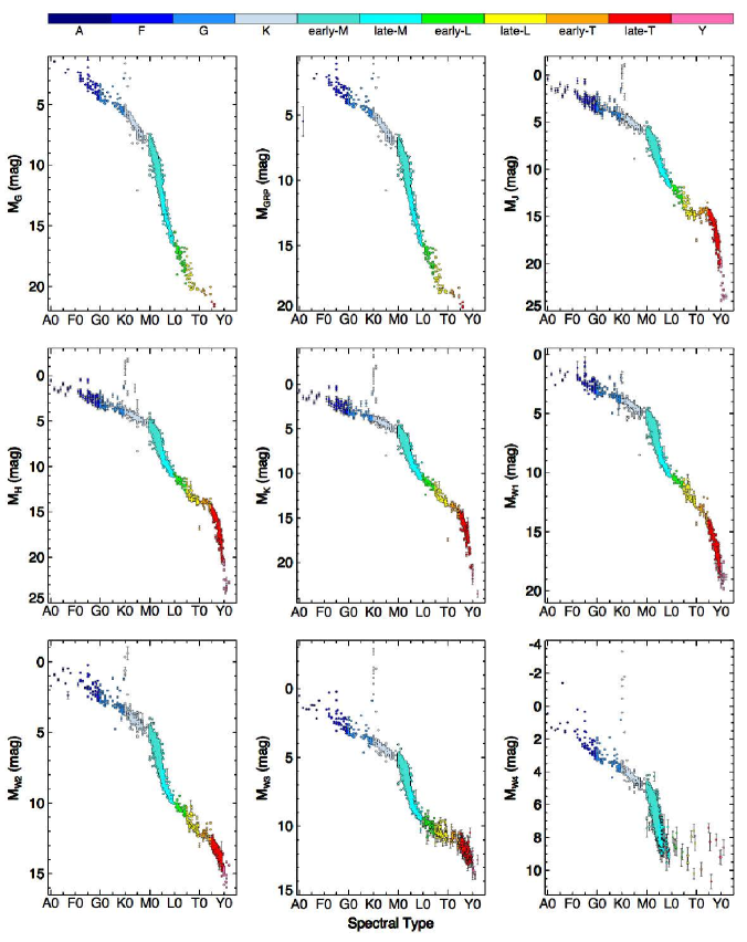
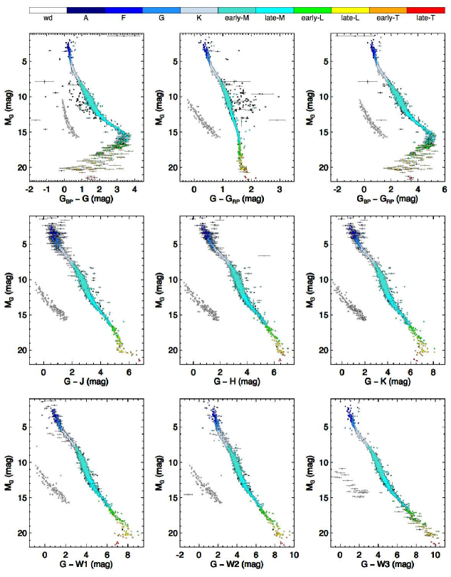
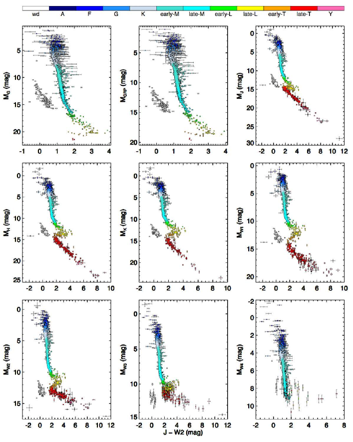
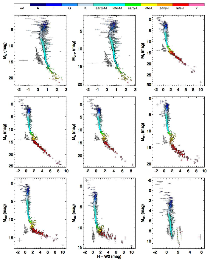
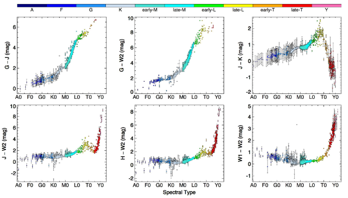
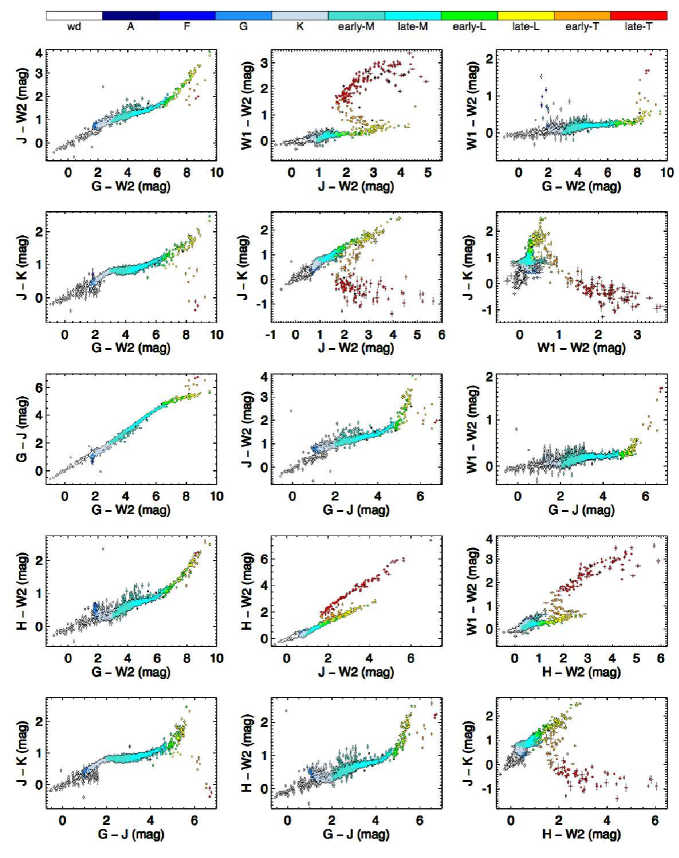
Each plot shows photometry only for those objects believed to be single components ("# Components this Row" = 1 in Table 3.1) and whose photometry is uncontaminated ("2MASS_contam?" and/or "WISE_contam?" not equal to "yes" in Table 3.1). Each object is color coded by its spectral type, as shown by the color bar in each figure303030This color palette was chosen so that each color could also be differentiated by readers with deuteranopia, protanopia, tritanopia, or achromatopsia.. Preference is given to the near-infrared spectral type if listed; otherwise, the optical spectral type is used. (It should be noted that for stars of type A through M, near-infrared classifications are given in Table 3.1 only when no optical type is available, so this criterion is only relevant for the L, T, and Y dwarfs.) Each object is plotted as a solid black dot, the center of which is colored if the spectral type is known; that is, objects lacking a spectral type appear only as black dots. Furthermore, for plots that involve or bands, preference is given to MKO magnitudes; otherwise 2MASS magnitudes are used.
In Figure 4, only those objects with absolute magnitude uncertainties below 1.0 mag are shown, to keep the plots more legible. In Figure 5, objects are shown only if their uncertainties in are below 1.0 mag and their color uncertainties are below 0.5 mag. In Figure 6 (or 7), objects are shown only if their absolute magnitude uncertainties are below 1.0 mag and their W2 (or W2) uncertainties are also below 1.0 mag. In Figure 8, objects are shown only if the color uncertainty is less than 0.5 mag for Gaia-based color plots or less than 1.0 mag for all other colors. In Figure 9, points are shown only if their color uncertainties are generally less than 0.10-0.20 mag.
We have examined each of these diagrams in detail and have identified objects that fall significantly far from the common loci of main sequence stars or white dwarfs to warrant special attention. There are several classes of objects, however, that we do not discuss in this section but address elsewhere: (1) Stars with bright magnitudes may be problematic and have quoted uncertainties insufficiently small to capture these problems. Given that these bright stars are generally well characterized already, we concentrate only on those not believed to be main sequence stars (category #4 below). (2) L, T, and Y dwarfs have already been examined in detail via color-type, color-magnitude, and color-color diagrams in Kirkpatrick et al. (2021a). (3) Subgiant, giant, and bright giant stars are discussed in Section 6.1.2. (4) Low-metallicity (subdwarf) stars are discussed in Section 6.2.2. (5) Young objects are discussed in Section 6.2.1.
We begin with objects whose placement on these diagrams could potentially highlight a problem with their measured parallaxes. These are all objects that the Gaia survey is placing within the 20-pc volume for the first time. With the exception of the object at , all of these objects have higher than normal Gaia parallax uncertainties as compared to objects of similar magnitude. We discuss each of these individually below:
-
•
Gaia EDR3 4966072879648455296 (02293606): This object, whose spectral type has yet to be determined but whose Gaia eDR3/DR3 parallax is mas, falls near or just above the main sequence on most color-magnitude diagrams. Its apparent magnitudes are similar to 20-pc objects of the same color, so there is no reason to question its inclusion in our census. Its location on color-magnitude diagrams along with its high DR3 RUWE value of 5.438 indicate possible unresolved binarity.
-
•
Gaia EDR3 3330473222213987072 (0623+1018): This M3 dwarf (see Section A.2) has a Gaia eDR3/DR3 parallax of mas. The derived value is 8 magnitudes fainter than that expected for an average M3 dwarf, and the value is 9 magnitudes fainter. The Gaia parallax value for this object is clearly in error, so it has been removed from the 20-pc census.
-
•
Gaia EDR3 3460907947316392704 (11593634): This is an M9.5 dwarf with a Gaia eDR3/DR3 parallax of mas. Its apparent magnitudes fall within the range of other M9.5 dwarfs within the 20-pc census. In absolute magnitude, it falls above the main sequence by as much as a magnitude for objects of similar color, and its Gaia RUWE value is 1.482. This position on color-magnitude diagrams cannot be explained by binarity alone, but a slightly larger parallax in tandem would solve the discrepancy. In any event, there is no reason to exclude this object from Table 3.1.
-
•
Gaia EDR3 6025146733201615616 (16243212): This object, of unknown type, has a Gaia eDR3/DR3 parallax of mas. Its apparent magnitude falls in the range expected for objects of similar color within 20 pc. On plots of absolute magnitude vs. color, however, it appears anomalous. On the vs. plot, it falls 0.4 mag more luminous than objects of similar color; on the vs. plot, it is also more luminous, but by 2.4 mag. Whether these issues indicate a problem with the measured photometry, the measured astrometry, or both – or whether the object has an unusual spectrum – is currently unknown. This object is retained in Table 3.1.
-
•
Gaia DR2 4062191480304598656 (AB) (17362515): This object, also of unknown type, has a Gaia DR2 parallax of mas and is a known double (Vrijmoet et al. 2022). Gaia DR3 lists two sources near this position, but neither have a parallax or proper motion measurement. The apparent magnitude of the DR2 source is at odds with the range expected for objects of similar color within 20 pc for many combinations of apparent magnitude vs. color, such as vs. W2, vs. W2, and vs. . The object also has a very small Gaia-measured proper motion of mas yr-1 and lies near the Galactic Center at . This object is most likely a background object with a faulty parallax, so we have removed it from the 20-pc census.
-
•
Gaia DR2 1795813379365971072 (2151+2328): No spectrum has been acquired of this object, and it appears to be a very close double in both Gaia DR2 and eDR3/DR3. However, only one of these components has a parallax measurement in DR2, and neither one does in DR3. This object lies well below and blueward of the main sequence on many apparent magnitude vs. color plots such as vs. , W2 vs. , and vs. W2. The object also has a small Gaia DR2 motion of only mas yr-1. This is likely a background source with a bogus parallax, so we have removed it from the 20-pc census.
The rest of our analysis deals with objects that are outliers for various other reasons. As discussed below, these reasons include possible unresolved binarity, unusual atmospheric composition, variability corrupting pan-epoch colors, and suspected typographical errors in published literature values.
-
•
HD 1237 B (00167951): For its spectral type of M4, this object has and colors much bluer than expected, while its color is much redder than expected. No other separate photometry of the B component is given in Table 3.1. Given that the A component is eight magnitudes brighter in than the B component and lies only away, we suspect a problem with the measured photometry of B that is not adequately reflected in its quoted uncertainties.
-
•
EGGR 246 (00412221): This is an oddly blue white dwarf in colors that use W1 or W2 magnitudes. The object is also blue relative to other white dwarfs in color, though normal in . This carbon-bearing object has a peculiar spectral type, DQpec9.3, and is believed to have a mixed hydrogen-helium atmosphere. The known infrared flux deficit is thought to be caused by absorption by H2 via collisions with neutral He (Giammichele et al. 2012; Bergeron et al. 1994, 2022).
-
•
LP 941-19 (02133345): Although this DA4.5 white dwarf has contaminated WISE photometry, it falls in an odd position on plots based only on Gaia photometry. Specifically, at its value of it falls 0.5 mag blueward of the white dwarf locus in and 0.3 mag redward in . There is very little literature on this source, and our spectrum of it (Section A.2) is the first published. It is not yet clear if this spectrum differs markedly enough from other DA white dwarfs to account for the color discrepancies or whether the Gaia magnitudes themselves are at fault.
-
•
HD 21209 A (03234959): The only oddity with this K dwarf is its anomalously blue W1W2 color. The value in Table 3.1, which is from the WISE All-Sky Source Catalog, is W1W2 = mag. Although this is the preferred WISE catalog for sources of this brightness (W1 = 5.56 mag), the AllWISE Source Catalog gives a very similar color of W1W2 = mag. This color may be due to the slightly subsolar metallicity of the object ([Fe/H]=, Soto & Jenkins 2018; , Sousa et al. 2008; , Tsantaki et al. 2013).
-
•
HD 23189 (0348+6840): This early-K dwarf is underluminous for its type at , , , , and . When colors formed from Gaia-based magnitudes are compared to the mean colors of objects of the same type, it appears normal, whereas the W1W2 color is slightly bluer than normal. We suspect that the Gray et al. (2003) type of K2 V is a typographical error, as independent assessments of the type from spectra, colors, and luminosity considerations (Adams et al. 1935; Bidelman 1985; Mermilliod 1987; Stassun et al. 2019) suggest a spectral type closer to K7.
-
•
2MASS J05053461+4648017 (0505+4648): This is an M8 dwarf (see Section A.2) with a Gaia DR3 parallax value of mas. The absolute values calculated with this parallax are similar to those of other known M8 dwarfs in the census, and a previous parallax of mas (Dittmann et al. 2014) also places it within 20 pc. Its location on color-magnitude diagrams such as vs. W2 along with its high DR3 RUWE value of 4.823 indicate possible unresolved binarity.
-
•
DENIS J071807.3350220 (07183502): On the and vs. various absolute magnitude diagrams, this object appears to be 0.7 mag above the locus of other objects of the same color. This is, therefore, likely a near equal-magnitude double. This object is also flagged as a possible binary in the Apps Catalog, again based on its position in color-magnitude diagrams.
-
•
SCR J08183110 (08183110): This DZ white dwarf is an outlier on the vs. W1W2 diagram and, in fact, any diagram involving W1W2 color. This issue has been hinted at previously in Figure 4 of Kawka et al. (2021), which shows that the best model fit to existing spectra and photometry fails to match the observed W1W2 color. Although the effect is known, its reason has apparently not yet been established and may be caused by variability or missing opacity sources in the models.
-
•
UPM J09016526 (09016526): This K5 dwarf is an outlier on all plots showing spectral type but appears normal on color-color and color-magnitude plots. We suggest that the published type of K5 (Riaz et al. 2006) results from a transcription error in the data for this star and that the actual spectral type is closer to M5.
-
•
APMPM J12512121 (12502121): This M6/6.5 dwarf has a Gaia DR3 parallax of mas. Its apparent magnitudes fall within the range expected for an M6 dwarf within the 20-pc volume, and a previous parallax measurement of mas (Winters et al. 2015) is in agreement with the Gaia one. On the vs. diagram, it falls 0.5 mag above the main sequence, and on the vs. W2 diagram, it falls 0.7 mag above. This and the Gaia DR3 RUWE value of 2.888 suggest unresolved binarity.
-
•
HD 113194 (13022647): Although this K5 dwarf has a Gaia DR3 parallax with a relatively large uncertainty ( mas), the earlier Hipparcos parallax ( mas) is in agreement. This object also has a high Gaia DR3 RUWE value, is listed as a high-LUWE object (see Section 5.2), and shows acceleration (see Section 4.1.4), in addition to falling 0.5 mag above the main sequence on the vs. diagram. This object is almost certainly an unresolved binary. It is also considered to be binary in the Apps Catalog, based on its position on color-magnitude diagrams. The Gaia DR3 main catalog reports a radial velocity of km s-1 using seventeen observations over 920 days, along with an amplitude of radial velocity variations of 60.25 km s-1, further supporting the hypothesis of binarity. The P-value for radial velocity constancy (rv_chisq_pvalue) is also 0.0.
-
•
2MASSW J1421314+182740 (1421+1827): This M9.5 dwarf has WISE photometry contaminated by a background source, but it appears unusual in non-WISE colors as well. Specifically, it has oddly blue and colors compared to other objects of similar . However, it appears normal for its in , , , and . This may simply indicate an issue with the magnitude that the formal uncertainty fails to adequately capture.
-
•
LP 222-65 (1516+3910): This mid-M dwarf lies consistently 0.6 mag above the main sequence relative to objects of the same color and spectral type on color-magnitude diagrams. This is an isolated object with no obvious problems with its photometry, so we believe this is an unresolved near-equal magnitude binary.
-
•
UCAC4 554-051865 (1518+2036): This mid-M dwarf is 0.6 mag more luminous than objects of similar color on the vs. and vs. diagrams and has a large RUWE and LUWE value (see Section 5.2). It is likely an unresolved binary.
-
•
L 339-19 (16404559): This M3 dwarf shows anomalously red W3 and W3 colors for its absolute magnitude, and even more anomalously red W4 and W4 colors. A more careful look at the WISE images shows that the W3 detection is likely real, but the W4 detection likely is not. The W3 photometry from AllWISE (reported in Table 3.1) is 7.100.05 mag and that from WISE All-Sky is 6.570.04 mag. In W3 and using the AllWISE value, the object lies 1.0 mag redward of objects of the same absolute magnitude; using the WISE All-Sky value shows the object to lie 0.5 mag redward. Archival Spitzer/IRAC and Spitzer/MIPS photometry of this object exists in the GLIMPSE I Spring ’07 Catalog (Benjamin et al. 2003) and MIPSGAL Archive (Carey et al. 2009) at IRSA: ch1 = 7.8300.038, ch2 = 7.7810.045, ch3 = 7.7240.037 (5.8 m), ch4 = 7.7050.026 (8.0 m), and [24m] = 7.140.24 mag. Running these new data points and the tabulated Table 3.1 photometry through the Virtual Observatory Spectral energy distribution Analyzer (VOSA313131http://svo2.cab.inta-csic.es/theory/vosa/; Bayo et al. 2008) suggests not only that the W4 magnitude is in error but that the W3 magnitude is spuriously bright relative to the bracketing IRAC and MIPS data points. The spectral energy distribution is otherwise typical of that of an M3 dwarf. We therefore conclude that there is no infrared excess in this object.
-
•
UCAC4 317-104829 (17062643): This DAH white dwarf is normal in Gaia-only colors, colors formed using Gaia minus near-infrared magnitudes, and colors formed from , , and magnitudes. It is, however, oddly blue in W1W2. We assume that this anomalous color may be intrinsic to the star and a result of its strong magnetic field, although it should be cautioned that this white dwarf is located against a busy region of the Galactic Plane and may suffer from contamination in its WISE photometry.
-
•
DENIS-P J1733423165449 (17331654): This L1 dwarf has WISE photometry that is contaminated by background sources, but it also shows unusual colors in Gaia-only measurements. Gaia DR3 lists two other point sources within of this object, so its Gaia photometry may be adversely affected in a way that the formal uncertainties fail to capture.
-
•
LSPM J1733+1655 (1733+1655): The Gaia DR3 parallax of mas has a relatively large uncertainly for its magnitude and is in disagreement with an earlier published value of mas by Dittmann et al. (2014). This mid-M dwarf is more luminous than objects of similar color by 1.6 mag on the vs. , , , , and W2 diagrams, if the Gaia DR3 parallax is used. This overluminosity decreases to 0.9 mag if the Dittmann et al. (2014) parallax is used instead. This is a high-RUWE/LUWE object as well (Section 5.2), and so is likely an unresolved multiple system with problematic Gaia astrometry. Clark et al. (2022) identify a candidate companion at separation and position angle 101∘ at epoch 2017.3 and again at separation and position angle 63∘ at epoch 2019.7. C. Gelino also finds a single epoch of Keck/NIRC2 data in the Keck Observatory Archive for LSPM J1733+1655. These are Br and -continuum observations taken on 2015 Jul 10 UT (PI: Hansen; Program ID: U050N2), from which we measure a separation of at position angle 248∘. If we assume all three of these measurements refer to the same star and it is a stationary background object, we derive motions of LSPM J1733+1655 of in RA and in Dec, which can be compared to the measured Gaia DR3 values of in RA and in Dec. The derived magnitude and direction of motion lead us to conclude that the background star hypothesis is sound.
-
•
LP 388-55 A (1735+2634): This late-M dwarf is anomalously red, by 0.25 mag, in color but looks normal in the color compared to objects of similar magnitude. Curiously, all Gaia-based absolute magnitudes (, , and ) are consistent with the reported spectral type. The B component is an early-L that is not directly imaged by Gaia but may nonetheless be subtly affecting the Gaia magnitudes of the A component.
-
•
LP 44-334 A (1840+7240): This primary in a M6.5 dwarf system has a Gaia DR3 parallax ( mas) with a relatively large uncertainty for its magnitude, but this value compares favorably to the earlier published value of mas by Lépine et al. (2009). The color is too blue for its value, the color is normal, and the color is too red. These issues are likely caused by the nearness of the B component, only away, which is likely corrupting the photometry of the A component.
-
•
LP 867-15 (18422328): The colors for this M0 dwarf are more consistent with an M4 dwarf than with an M0. Pending spectroscopic verification, we assume that this object has been misclassified.
-
•
SCR J20125956 (20125956): This object, a DC9.9 white dwarf, falls below the white dwarf locus for most colors. It is very blue relative to other white dwarfs in , , and but looks like other white dwarfs in colors made with Gaia-only magnitudes. It is somewhat blue in , , and colors. As with EGGR 246 above, the infrared flux deficit is believed to be caused by H2-He collision-induced absorption (Giammichele et al. 2012).
-
•
LEHPM 2-783 (20195816): This M6.5 dwarf is overluminous in all Gaia-based colors. (Many other colors are nearly degenerate with absolute magnitude or type in this spectral type range.) On both the vs. and the W2 vs. plots, the overluminosity is 0.7 mag. Ujjwal et al. (2020) mark this as a possible member of the Pic Moving Group, and Riaz et al. (2006) note that it is a strong X-ray emitter with strong H emission.
-
•
LP 12-90 (2322+7847): This mid-M dwarf lies above the main sequence by 0.75 mag on the vs. plot. On many other plots of absolute magnitude vs. color, it lies similarly above (and redward of) the main sequence. This could be another unresolved binary – if confirmed, this would make its system with HD 220140 AB a quadruple – but the primary in this system is a young, naked T Tauri star (Makarov et al. 2007), meaning that its position may be solely due to its youth.
-
•
ZZ Psc (2328+0514): This white dwarf is anomalously red in colors involving WISE magnitudes – so much so that it falls far from the white dwarf sequence itself. On a plot of vs. W1W2, for example, it lies substantially redward of both the white dwarf locus and the main sequence. This object, also known as G 29-38, is known to have a debris disk around it, the first evidence of which was uncovered by Zuckerman & Becklin (1987). For an update on this object, see Cunningham et al. (2022).
6 Masses from Estimation
Only a small fraction of objects within the 20-pc census has masses measurable by methods 1 or 2 described in the introduction of Section 4. For the rest, we must rely on methods 3 and 4 of that section, which depend on comparison to empirical trends or to theoretical models.
In the first subsection below, we discuss mass measurements for objects not on the main sequence – namely, white dwarfs, giants/subgiants, and brown dwarfs. In the second subsection, we summarize mass estimation for main sequence stars. In the third subsection, we discuss other complications – youth, subsolar metallicity, and formation scenario – that may need to be considered when assigning accurate mass estimates for special objects.
6.1 Individual objects not on the main sequence
6.1.1 White dwarfs
Masses have been measured via one of the methods described in Section 4 for a handful of white dwarfs in the 20-pc census, but these represent the end-state masses of the stellar remnants and are not suitable for analysis of the initial mass function. Rather, what is needed are the initial masses before evolution off the main sequence. Techniques have been established that use the final mass of the remnant to estimate the initial mass of the progenitor.
For white dwarfs lacking a direct mass measurement, one can estimate the final mass of the white dwarf using one of the following two semi-empirical methods. The first is to use spectroscopic observations of the depth and width of the hydrogen Balmer, He I, or He II lines to establish, after comparison to atmospheric models, the and for each object. Further comparison of these two parameters to cooling models provides the remnant mass (e.g., Tremblay et al. 2011; Genest-Beaulieu & Bergeron 2019; Bergeron et al. 1992; Finley et al. 1997). Whereas this first method is applicable only to DA (hydrogen atmosphere) or DB (helium atmosphere) white dwarfs, an alternate method can be used both for objects lacking hydrogen lines as well as for objects lacking spectroscopic observations. In this second method, masses can still be estimated if an accurate parallax has been measured. Here, absolute fluxes across as wide a swath of wavelength space as possible are compared to model atmospheres to provide and , from which the mass can be derived from equation 11 (e.g., Bergeron et al. 2019; Tremblay et al. 2019; Giammichele et al. 2012; Bergeron et al. 2001; Koester et al. 1979).
The next step is to convert this final mass into an initial mass using an initial-to-final mass relation (e.g., Weidemann 2000). The empirical form of this relationship has been established using white dwarfs that are members of open clusters of known age. As described above, spectroscopic observations of the Balmer lines in these stars can be compared to atmospheric models to derive and for each object. A comparison of these parameters to cooling models provides both the remnant mass as well as the cooling time since the object left the tip of the asymptotic giant branch. The known cluster age minus this cooling time gives the main sequence lifetime of the object, which can then be related back to an initial mass using theoretical evolutionary isochrones. This same technique can also be applied to white dwarfs in globular clusters. Due to their much older ages, these clusters can provide white dwarfs of lower final mass than those available in young open clusters. Because these globular clusters are much more distant, their white dwarfs are faint and more difficult to study, so old low-mass white dwarfs are still not well represented by cluster methods.
This lack of low-mass examples can be partly mitigated by the use of old, wide binaries for which the second component can be age dated and the separation between components is large enough that no mass transfer has occurred during the system’s evolution. Examples are wide subgiant + white dwarf binaries in which the system can be dated from its more recently evolved member (Barrientos & Chanamé 2021), wide F/G/K dwarf + white dwarf binaries in which the age of the main sequence star can be estimated from activity diagnostics (Catalán et al. 2008, Zhao et al. 2012), and white dwarf pairs in which comparison of the higher-mass white dwarf to known cluster white dwarfs can provide an age for the binary, and the difference in the cooling times for the white dwarf pair gives the main sequence lifetime of the lower-mass white dwarf (Andrews et al. 2015). Using the results of these methods, the trend of final mass with initial mass can be fit. As can be seen from figure 9 of Barrientos & Chanamé (2021), the relation shows considerable scatter at lower masses, as the age dating methods for individual systems are generally less robust than those from clusters. The relations we adopt here are the cluster-based tripartite parameterization found in equations 4-6 of Cummings et al. (2018) and the quadripartite parameterization found in table 1 of El-Badry et al. (2018), The former relation is applicable to white dwarfs with (), and the latter relation, which is based on nearby white dwarfs with accurate Gaia parallaxes, is applicable to white dwarfs with (). We further note that neither the cluster nor field methods have yet extended the initial-to-final mass relation below final masses of . (As discussed further below, white dwarfs with final masses below require binary interactions, as a single progenitor would imply an age older than the Universe; Marsh et al. 1995).
Specifically, we apply the following methodology to assign final masses to white dwarfs in the 20-pc census. First, we use directly measured masses, whenever such measurements are available. For others, we use final mass estimates that are based on accurate parallaxes, high S/N spectra, and/or broad-wavelength data spanning the white dwarf’s spectral energy distribution. For all other objects, we resort to the Gaia-centric estimates of Gentile Fusillo et al. (2021) and Gentile Fusillo et al. (2019). These estimates use only a small fraction of the white dwarf’s spectral energy distribution – spanning the Gaia optical bandpasses – and thus lead to separate solutions for hydrogen- vs. helium-atmosphere objects. When our own follow-up has determined the spectral type of the object, we use this information to break the degeneracy; otherwise, a hydrogen-atmosphere object is assumed, as noted in Table 6.1.1.
| Name | Abbrev. | WD | Final | Final | Ref. | Initial | Initial | Initial | Initial |
|---|---|---|---|---|---|---|---|---|---|
| Coords | NameaaWhite dwarf designations from McCook & Sion (2016). Those in parentheses are "WD" designations found in SIMBAD but not in McCook & Sion (2016). | Mass | Mass | Mass | Mass | Mass | Mass | ||
| (J2000) | () | Method | (Cummings)bbThe initial mass derived using the initial-to-final mass relation of Cummings et al. (2018). Uncertainties are derived by propagating the listed uncertainty for the final mass and the uncertainties listed for the coefficients of the initial-to-final mass relations in equations 4-6 of Cummings et al. (2018). | (El-Badry)ccThe initial mass derived using the initial-to-final mass relation of El-Badry et al. (2018). One-sigma uncertainties are chosen to match the initial mass 95.4% (2-sigma) envelope shown in figure 3 of El-Badry et al. (2018). | (Adopted)ddThis is our adopted initial mass. When both a Cummings et al. (2018) estimate and an El-Badry et al. (2018) estimate are available, this adopted mass in the unweighted average of those two. | Method | |||
| () | () | () | |||||||
| (1) | (2) | (3) | (4) | (5) | (6) | (7) | (8) | (9) | (10) |
| LAWD 96 | 00024309 | WD 2359434 | 0.780.03 | Spec | 1 | 3.21.5 | 3.40.2 | 3.31.5 | IFMR |
| LAWD 1 | 00023413 | WD 0000345 | 0.880.10 | Phot | 1 | 3.81.3 | 4.70.3 | 4.31.3 | IFMR |
| LP 464-57 | 0007+1230 | WD 0004+122 | 0.570.15 | Phot | 2 | 1.01.9 | 1.70.1 | 1.41.9 | IFMR |
| EGGR 381 | 0012+5025 | WD 0009+501 | 0.730.04 | Phot | 1 | 2.91.4 | 3.10.2 | 3.01.5 | IFMR |
| L 50-73 | 00137149 | WD 0011721 | 0.590.00 | Phot | 1 | 1.30.5 | 1.90.1 | 1.60.5 | IFMR |
| G 158-45 | 00141311 | WD 0011134 | 0.720.07 | Phot | 1 | 2.91.5 | 3.00.2 | 3.01.5 | IFMR |
| EGGR 246 | 00412221 | WD 0038226 | 0.530.01 | Phot | 1 | 1.30.1 | 1.30.1 | IFMR | |
| Wolf 28 | 0049+0523 | (WD 0046+051) | 0.680.02 | Phot | 1 | 2.40.7 | 2.80.2 | 2.60.7 | IFMR |
| Wolf 1516 | 0118+1610 | WD 0115+159 | 0.690.04 | Phot | 1 | 2.50.8 | 2.90.2 | 2.70.8 | IFMR |
| LP 991-16 A | 01244240 | WD 0121429 | 0.410.01eeQuoted mass estimate assumes the system is a single white dwarf. | Phot | 1 | 1.90.9 | Ultra-low | ||
| LP 991-16 B | 01244240 | 1 | 1.90.9 | Ultra-low | |||||
| EGGR 307 | 01252600 | WD 0123262 | 0.580.00 | Phot | 1 | 1.10.4 | 1.80.1 | 1.50.4 | IFMR |
| LAWD 10 A | 01370459 | WD 0135052.1 | 0.47 | Orbit | 4 | 1.00.1 | Low | ||
| LAWD 10 B | 01370459 | WD 0135052.2 | 0.52 | Orbit | 4 | 1.20.1 | 1.20.1 | IFMR | |
| L 88-59 | 01436718 | WD 0141675 | 0.480.06 | Spec | 1 | 1.00.1 | Low | ||
| EGGR 268 | 0151+6425 | WD 0148+641 | 0.810.01 | GravRed | 5 | 3.31.5 | 3.50.2 | 3.41.5 | IFMR |
| GD 279 | 0152+4700 | WD 0148+467 | 0.630.03 | Spec | 1 | 1.80.6 | 2.30.2 | 2.10.7 | IFMR |
| Eri B | 01555136 | - | 1.90.9 | Conjecture | |||||
| HD 13445 B | 02105049 | WD 0208510 | 0.5970.010 | Accel | 6 | 1.40.5 | 2.00.1 | 1.70.5 | IFMR |
| EGGR 168 | 0211+3955 | WD 0208+396 | 0.480.10 | Spec | 7 | 1.00.1 | Low | ||
| LP 649-66 | 02120804 | 0.530.02 | Gaia H-atm* | 8 | 1.30.1 | 1.30.1 | IFMR | ||
| LP 941-19 | 02133345 | 0.370.05 | Gaia H-atm* | 8 | 1.90.9 | Ultra-low | |||
| EGGR 471 | 02321411 | WD 0230144 | 0.660.06 | Phot | 1 | 2.10.9 | 2.70.2 | 2.41.0 | IFMR |
| LP 830-14 | 02352400 | WD 0233242 | 0.580.00 | Phot | 1 | 1.10.4 | 1.80.1 | 1.50.4 | IFMR |
| EGGR 473 | 0248+5423 | WD 0245+541 | 0.730.03 | Phot | 1 | 2.91.4 | 3.10.2 | 3.01.5 | IFMR |
| CPD69 177 | 03106836 | WD 0310688 | 0.670.03 | Spec | 1 | 2.30.7 | 2.80.2 | 2.50.7 | IFMR |
| For Bb | 03122859 | - | 1.90.9 | Conjecture | |||||
| EGGR 566 | 03250149 | WD 0322019 | 0.630.05 | Phot | 1 | 1.80.8 | 2.30.2 | 2.10.8 | IFMR |
| Wolf 219 | 0344+1826 | WD 0341+182 | 0.570.06 | Phot | 1 | 1.00.9 | 1.70.1 | 1.40.9 | IFMR |
| G 7-16 | 0400+0814 | WD 0357+081 | 0.610.06 | Phot | 1 | 1.50.9 | 2.10.2 | 1.80.9 | IFMR |
| Eri B | 04150739 | (WD 0413077) | 0.5730.018 | Orbit | 9 | 1.10.5 | 1.70.1 | 1.40.5 | IFMR |
| Ret B | 04165917 | WD 0415594 | 0.600.12 | Spec | 7 | 1.41.6 | 2.00.2 | 1.71.6 | IFMR |
| EGGR 169 | 0425+1211 | WD 0423+120 | 0.650.04 | Phot | 1 | 2.00.7 | 2.60.2 | 2.30.8 | IFMR |
| EGGR 180 | 0431+5858 | WD 0426+588 | 0.6750.051 | Lensing | 10 | 2.30.9 | 2.80.2 | 2.60.9 | IFMR |
| HD 283750 B | 0436+2709 | WD 0433+270 | 1.120.01 | GravRed | 5 | 6.11.2 | 6.50.4 | 6.31.2 | IFMR |
| EGGR 41 | 04370849 | WD 0435088 | 0.530.02 | Phot | 1 | 1.30.1 | 1.30.1 | IFMR | |
| LP 777-1 | 05051722 | WD 0503174 | 0.530.01 | Spec | 23 | 1.30.1 | 1.30.1 | IFMR | |
| V371 Ori B | 0533+0156 | 0.630.17 | Dyn+mod | 18 | 1.82.2 | 2.30.2 | 2.12.2 | IFMR | |
| EGGR 248 | 05510010 | WD 0548001 | 0.690.03 | Phot | 1 | 2.50.7 | 2.90.2 | 2.70.8 | IFMR |
| UCAC4 398-010797 | 05541035 | 0.680.01 | Gaia He-atm | 8 | 2.40.6 | 2.80.2 | 2.60.7 | IFMR | |
| EGGR 45 | 05550410 | WD 0552041 | 0.820.01 | Phot | 1 | 3.41.5 | 3.70.2 | 3.61.6 | IFMR |
| EGGR 290 | 0556+0521 | WD 0553+053 | 0.720.03 | Phot | 1 | 2.91.4 | 3.00.2 | 3.01.4 | IFMR |
| G 249-36 B | 0605+6049 | 1.030.08 | Dyn+mod | 21 | 5.21.3 | 5.90.4 | 5.61.4 | IFMR | |
| CMa B | 06451643 | WD 0642166 | 1.0170.025 | GravRed | 11 | 5.11.1 | 5.90.4 | 5.51.1 | IFMR |
| EGGR 484 | 0647+0231 | WD 0644+025 | 0.850.15 | Spec | 7 | 3.61.8 | 4.20.3 | 3.91.8 | IFMR |
| LAWD 23 | 0647+3730 | WD 0644+375 | 0.690.03 | Spec | 1 | 2.50.7 | 2.90.2 | 2.70.8 | IFMR |
| L 454-9 | 06573909 | WD 0655390 | 0.590.00 | Phot | 1 | 1.30.5 | 1.90.1 | 1.60.5 | IFMR |
| EGGR 485 | 0700+3157 | WD 0657+320 | 0.600.02 | Phot | 1 | 1.40.5 | 2.00.2 | 1.70.6 | IFMR |
| SCR J07086706 | 07086706 | WD 0708670 | 0.570.00 | Phot | 1 | 1.00.4 | 1.70.1 | 1.40.4 | IFMR |
| EGGR 52 A | 0730+4810 | WD 0727+482A | 0.510.01 | Phot | 1 | 1.10.1 | 1.10.1 | IFMR | |
| EGGR 52 B | 0730+4810 | WD 0727+482B | 0.650.01 | Phot | 1 | 2.00.6 | 2.60.2 | 2.30.6 | IFMR |
| EGGR 321 | 0733+6409 | WD 0728+642 | 0.580.00 | Phot | 1 | 1.10.4 | 1.80.1 | 1.50.4 | IFMR |
| CMi B | 0739+0513 | WD 0736+053 | 0.5530.022 | Orbit | 13 | 1.50.1 | 1.50.1 | IFMR | |
| LAWD 25 | 07401724 | WD 0738172 | 1.110.05 | GravRed | 5 | 6.01.2 | 6.40.4 | 6.21.3 | IFMR |
| VB 3 | 07453355 | (WD 0743336) | 0.550.01 | Phot | 1 | 1.50.1 | 1.50.1 | IFMR | |
| EGGR 426 | 0750+0711 | WD 0747+073.1 | 0.480.01 | Phot | 1 | 1.00.1 | Low | ||
| EGGR 427 | 0750+0711 | WD 0747+073.2 | 0.560.01 | Phot | 1 | 0.90.4 | 1.60.1 | 1.20.4 | IFMR |
| LAWD 26 | 07536747 | WD 0752676 | 0.730.06 | Phot | 1 | 2.91.5 | 3.10.2 | 3.01.5 | IFMR |
| SCR J075-2524 | 07532524 | WD 0751252 | 0.520.01 | Gaia-H | 8 | 1.20.1 | 1.20.1 | IFMR | |
| L 97-3 A | 08066618 | WD 0806661 | 0.580.03 | Phot | 1 | 1.10.6 | 1.80.1 | 1.50.6 | IFMR |
| UPM J08123529 | 08123529 | (WD 0810353) | 0.700.01 | Gaia H-atm* | 8 | 2.60.7 | 2.90.2 | 2.80.7 | IFMR |
| G 111-64 | 0814+4845 | WD 0810+489 | 0.570.00 | Phot | 1 | 1.00.4 | 1.70.1 | 1.40.4 | IFMR |
| SCR J08183110 | 08183110 | WD 0816310 | 0.570.00 | Phot | 1 | 1.00.4 | 1.70.1 | 1.40.4 | IFMR |
| SCR J08216703 | 08216703 | WD 0821669 | 0.660.01 | Phot | 1 | 2.10.6 | 2.70.2 | 2.40.6 | IFMR |
| CD32 5613 | 08413256 | WD 0839327 | 0.450.05 | Spec | 7 | 1.00.1 | Low | ||
| LP 726-1 | 08421347 | WD 0840136 | 0.570.00 | Phot | 1 | 1.00.4 | 1.70.1 | 1.40.4 | IFMR |
| UMa Ab | 0859+4802 | 1.000.30 | Dyn+mag | 19 | 4.93.0 | 5.80.4 | 5.33.0 | IFMR | |
| LP 606-32 | 08590058 | WD 0856007 | 0.520.01 | Gaia He-atm | 8 | 1.20.1 | 1.20.1 | IFMR | |
| EGGR 250 | 0915+5325 | WD 0912+536 | 0.750.02 | Phot | 1 | 3.01.5 | 3.20.2 | 3.11.5 | IFMR |
| EGGR 252 | 1001+1441 | WD 0959+149 | 0.700.01 | Gaia He-atm | 8 | 2.60.7 | 2.90.2 | 2.80.7 | IFMR |
| LP 315-42 | 1011+2845 | WD 1008+290 | 0.680.01 | Phot | 1 | 2.40.6 | 2.80.2 | 2.60.7 | IFMR |
| WT 1759 | 10121843 | WD 1009184 | 0.590.02 | Phot | 1 | 1.30.5 | 1.90.1 | 1.60.5 | IFMR |
| EGGR 350 | 1023+6327 | WD 1019+637 | 0.570.05 | Phot | 1 | 1.00.8 | 1.70.1 | 1.40.8 | IFMR |
| LP 37-186 | 1037+7110 | WD 1033+714 | 0.580.00 | Phot | 1 | 1.10.4 | 1.80.1 | 1.50.4 | IFMR |
| EGGR 535 | 10382040 | WD 1036204 | 0.600.01 | Phot | 1 | 1.40.5 | 2.00.2 | 1.70.5 | IFMR |
| BD18 3019 B | 10451906 | WD 1043188 | 0.530.11 | Phot | 1 | 1.30.1 | 1.30.1 | IFMR | |
| LAWD 34 | 10570731 | WD 1055072 | 0.850.04 | Phot | 1 | 3.61.6 | 4.20.3 | 3.91.6 | IFMR |
| UMa Bb | 1118+3131 | - | 1.90.9 | Conjecture | |||||
| SCR J11184721 | 11184721 | WD 1116470 | 0.570.00 | Phot | 1 | 1.00.4 | 1.70.1 | 1.40.4 | IFMR |
| Ross 627 | 1124+2121 | WD 1121+216 | 0.610.11 | Spec | 7 | 1.51.5 | 2.10.2 | 1.81.5 | IFMR |
| 20 Crt B | 11343250 | WD 1132325 | 0.600.01 | Gaia He-atm | 8 | 1.40.5 | 2.00.2 | 1.70.5 | IFMR |
| GD 140 | 1137+2947 | WD 1134+300 | 0.970.03 | Spec | 1 | 4.71.0 | 5.60.4 | 5.11.1 | IFMR |
| LAWD 37 | 11456450 | (WD 1142645) | 0.610.01 | Phot | 1 | 1.50.5 | 2.10.2 | 1.80.5 | IFMR |
| SSSPM J11487458 | 11477457 | 0.4880.003 | Gaia He-atm | 8 | 1.00.1 | Low | |||
| SDSS J115052.32+683116.1 | 1150+6831 | WD 1148+687 | 0.690.04 | Spec | 2 | 2.50.8 | 2.90.2 | 2.70.8 | IFMR |
| LP 852-7 | 12052333 | WD 1202232 | 0.590.03 | Spec | 1 | 1.30.6 | 1.90.1 | 1.60.6 | IFMR |
| G 197-47 | 1211+5724 | WD 1208+576 | 0.560.09 | Phot | 1 | 0.91.2 | 1.60.1 | 1.21.2 | IFMR |
| WG 21 | 12266612 | WD 1223659 | 0.450.02 | Spec | 1 | 1.00.1 | Low | ||
| WG 22 | 12384948 | WD 1236495 | 1.130.14 | Spec | 7 | 6.21.8 | 6.50.4 | 6.31.8 | IFMR |
| Wolf 457 | 1300+0328 | WD 1257+037 | 0.700.06 | Phot | 1 | 2.61.0 | 2.90.2 | 2.81.0 | IFMR |
| EGGR 436 | 1308+8502 | WD 1309+853 | 0.710.02 | Phot | 1 | 2.80.7 | 3.00.2 | 2.90.7 | IFMR |
| ER 8 | 13124728 | WD 1310472 | 0.630.04 | Phot | 1 | 1.80.7 | 2.30.2 | 2.10.7 | IFMR |
| LP 854-50 | 13192147 | WD 1316215 | 0.990.01 | Gaia H-atm | 8 | 4.91.0 | 5.70.4 | 5.31.1 | IFMR |
| LAWD 45 | 13197823 | WD 1315781 | 0.690.02 | Phot | 1 | 2.50.7 | 2.90.2 | 2.70.7 | IFMR |
| BD-07 3632 | 13300834 | WD 1327083 | 0.500.06 | GravRed | 5 | 1.00.1 | 1.00.1 | IFMR | |
| Wolf 489 | 1336+0340 | (WD 1334+039) | 0.540.03 | Phot | 1 | 1.40.1 | 1.40.1 | IFMR | |
| LSPM J1341+0500 | 1341+0500 | (WD 1338+052) | 0.580.15 | Phot | 2 | 1.11.9 | 1.80.1 | 1.51.9 | IFMR |
| EGGR 438 | 1348+2334 | WD 1345+238 | 0.450.02 | Phot | 1 | 1.00.1 | Low | ||
| PG 1350090 | 13530916 | WD 1350090 | 0.680.03 | Spec | 1 | 2.40.7 | 2.80.2 | 2.60.7 | IFMR |
| VVV J141159.32592045.7 | 14115920 | 0.660.01 | Gaia H-atm* | 8 | 2.10.6 | 2.70.2 | 2.40.6 | IFMR | |
| LP 801-9 | 14471742 | WD 1444174 | 0.820.05 | Phot | 1 | 3.41.6 | 3.70.2 | 3.61.6 | IFMR |
| G 137-24 | 1535+1247 | WD 1532+129 | 0.570.15 | Phot | 2 | 1.01.9 | 1.70.1 | 1.41.9 | IFMR |
| HD 140901 B | 15473755 | WD 1544377 | 0.580.01 | GravRed | 5 | 1.10.5 | 1.80.1 | 1.50.5 | IFMR |
| CD38 10980 | 16233913 | WD 1620391 | 0.650.01 | GravRed | 5 | 2.00.6 | 2.60.2 | 2.30.6 | IFMR |
| Ross 640 | 1628+3646 | WD 1626+368 | 0.580.03 | Phot | 1 | 1.10.6 | 1.80.1 | 1.50.6 | IFMR |
| G 138-38 | 1632+0851 | WD 1630+089 | 0.590.15 | Spec | 2 | 1.31.9 | 1.90.1 | 1.61.9 | IFMR |
| EGGR 258 | 1634+5710 | WD 1633+572 | 0.570.04 | Phot | 1 | 1.00.7 | 1.70.1 | 1.40.7 | IFMR |
| PG 1633+434 | 1635+4317 | WD 1633+433 | 0.680.04 | Phot | 1 | 2.40.8 | 2.80.2 | 2.60.8 | IFMR |
| DN Dra | 1648+5903 | WD 1647+591 | 0.770.03 | Astero | 14 | 3.11.5 | 3.30.2 | 3.21.5 | IFMR |
| UCAC4 317-104829 | 17062643 | (WD 1703267) | 0.8080.009 | Gaia H-atm | 8 | 3.31.5 | 3.50.2 | 3.41.5 | IFMR |
| EGGR 494 | 1708+0257 | WD 1705+030 | 0.680.09 | Phot | 1 | 2.41.3 | 2.80.2 | 2.61.3 | IFMR |
| G 203-47 B | 1709+4340 | WD 1708+437 | 0.50 | Dyn+mod | 22 | 1.4 | 2.0 | 1.4 | IFMR |
| PM J174765436 | 17475436 | 0.480.01 | Gaia He-atm | 8 | 1.00.1 | Low | |||
| EGGR 372 | 1748+7052 | WD 1748+708 | 0.790.01 | Phot | 1 | 3.21.5 | 3.40.2 | 3.31.5 | IFMR |
| EGGR 199 | 1749+8246 | WD 1756+827 | 0.550.13 | Spec | 7 | 1.50.1 | 1.50.1 | IFMR | |
| LSR J1817+1328 | 1817+1328 | WD 1814+134 | 0.680.02 | Phot | 1 | 2.40.7 | 2.80.2 | 2.60.7 | IFMR |
| G 227-28 | 1821+6101 | WD 1820+609 | 0.560.05 | Phot | 1 | 0.90.8 | 1.60.1 | 1.20.8 | IFMR |
| EGGR 176 | 18241308 | WD 1821131 | 1.060.07 | Spec | 3 | 5.51.3 | 6.10.4 | 5.81.3 | IFMR |
| UCAC4 508-079937 | 1825+1135 | 0.510.01 | Gaia H-atm | 8 | 1.10.1 | 1.10.1 | IFMR | ||
| EGGR 374 | 1830+5447 | WD 1829+547 | 0.900.07 | Phot | 1 | 4.01.1 | 5.00.3 | 4.51.2 | IFMR |
| LAWD 73 | 1900+7039 | WD 1900+705 | 0.930.02 | Phot | 1 | 4.31.0 | 5.30.3 | 4.81.0 | IFMR |
| EGGR 375 | 1918+3843 | WD 1917+386 | 0.750.04 | Phot | 1 | 3.01.5 | 3.20.2 | 3.11.5 | IFMR |
| LAWD 74 | 19200740 | WD 1917077 | 0.620.02 | Phot | 1 | 1.60.6 | 2.20.2 | 1.90.6 | IFMR |
| UCAC4 482-095741 | 1921+0613 | 0.680.01 | Gaia H-atm | 8 | 2.40.6 | 2.80.2 | 2.60.7 | IFMR | |
| GD 219 | 1921+1440 | WD 1919+145 | 0.740.03 | Spec | 1 | 3.01.4 | 3.10.2 | 3.11.5 | IFMR |
| PY Vul | 1937+2743 | WD 1935+276 | 0.660.02 | Astero | 15 | 2.10.6 | 2.70.2 | 2.40.7 | IFMR |
| LAWD 79 | 1956-0102 | WD 1953011 | 0.790.13 | Spec | 7 | 3.21.7 | 3.40.2 | 3.31.7 | IFMR |
| Wolf 1130 B | 2005+5426 | WD 2003+542 | 1.240.17 | Orbit | 16 | 7.22.0 | 7.20.4 | 7.22.1 | IFMR |
| EGGR 498 | 20051056 | WD 2002110 | 0.720.01 | Phot | 1 | 2.91.4 | 3.00.2 | 3.01.4 | IFMR |
| CD30 17706 | 20103013 | WD 2007303 | 0.600.02 | Spec | 1 | 1.40.5 | 2.00.2 | 1.70.6 | IFMR |
| SCR J20125956 | 20125956 | WD 2008600 | 0.440.01 | Phot | 1 | 1.90.9 | Ultra-low | ||
| EC 201733036 | 20203027 | 0.750.01 | Gaia H-atm* | 8 | 3.01.5 | 3.20.2 | 3.11.5 | IFMR | |
| HD 340611 | 2034+2503 | WD 2032+248 | 0.640.03 | Spec | 1 | 1.90.7 | 2.40.2 | 2.20.7 | IFMR |
| EGGR 140 | 20446805 | WD 2039682 | 0.980.03 | Spec | 1 | 4.81.0 | 5.60.4 | 5.21.1 | IFMR |
| EGGR 261 | 2049+3728 | WD 2047+372 | 0.810.03 | Spec | 1 | 3.31.5 | 3.50.2 | 3.41.5 | IFMR |
| G 187-8 A | 2050+2630 | WD 2048+263 | 0.240.04eeQuoted mass estimate assumes the system is a single white dwarf. | Phot | 1 | 1.90.9 | Ultra-low | ||
| G 187-8 B | 2050+2630 | 1 | 1.90.9 | Ultra-low | |||||
| UCAC4 325-215293 | 20522504 | (WD 2049253) | 0.470.01 | Gaia He-atm | 8 | 1.00.1 | Low | ||
| Ross 193 B | 20560450 | WD 2054050 | 0.490.01 | Spec | 23 | 1.00.1 | Low | ||
| WT 765 | 21014906 | 0.530.01 | Gaia H-atm | 8 | 1.30.1 | 1.30.1 | IFMR | ||
| LAWD 83 | 21138149 | WD 2105820 | 0.780.10 | Spec | 7 | 3.21.6 | 3.40.2 | 3.31.6 | IFMR |
| EGGR 378 | 2118+5412 | WD 2117+539 | 0.560.03 | Spec | 1 | 0.90.6 | 1.60.1 | 1.20.6 | IFMR |
| Oct B | 21417723 | 0.550.05 | Dyn+mod | 20 | 1.50.1 | 1.50.1 | IFMR | ||
| L 570-26 | 21413300 | WD 2138332 | 0.700.02 | Phot | 1 | 2.60.7 | 2.90.2 | 2.80.7 | IFMR |
| EGGR 148 | 2142+2059 | WD 2140+207 | 0.480.04 | Phot | 1 | 1.00.1 | Low | ||
| PHL 1716 | 21430659 | 0.870.01 | Gaia H-atm | 8 | 3.70.9 | 4.50.3 | 4.11.0 | IFMR | |
| UCAC4 747-070768 | 2151+5917 | (WD 2150+591) | 0.570.01 | Gaia H-atm | 8 | 1.00.4 | 1.70.1 | 1.40.5 | IFMR |
| WG 39 | 21575100 | WD 2154512 | 0.600.04 | Phot | 1 | 1.40.7 | 2.00.2 | 1.70.7 | IFMR |
| CD Oct | 22047513 | WD 2159754 | 0.920.04 | Spec | 1 | 4.21.0 | 5.30.3 | 4.71.1 | IFMR |
| WD 2211392 | 22143859 | WD 2211392 | 0.800.04 | Phot | 1 | 3.31.5 | 3.50.2 | 3.41.5 | IFMR |
| SCR J22307515 | 22307515 | WD 2226755 | 0.580.00 | Phot | 1 | 1.10.4 | 1.80.1 | 1.50.4 | IFMR |
| SCR J22307513 | 22307513 | WD 2226754 | 0.580.00 | Phot | 1 | 1.10.4 | 1.80.1 | 1.50.4 | IFMR |
| EGGR 155 | 2249+2236 | WD 2246+223 | 1.110.21 | Spec | 7 | 6.02.3 | 6.40.4 | 6.22.3 | IFMR |
| EGGR 283 A | 2251+2939 | WD 2248+293 | 0.350.07eeQuoted mass estimate assumes the system is a single white dwarf. | Phot | 1 | 1.90.9 | Ultra-low | ||
| EGGR 283 B | 2251+2939 | 1 | 1.90.9 | Ultra-low | |||||
| EGGR 453 | 22530646 | (WD 2251070) | 0.580.03 | Phot | 1 | 1.10.6 | 1.80.1 | 1.50.6 | IFMR |
| LSPM J2309+5506E | 2309+5506 | WD 2307+548 | 0.590.15 | Spec | 2 | 1.31.9 | 1.90.1 | 1.61.9 | IFMR |
| ZZ Psc | 2328+0514 | WD 2326+049 | 0.5930.012 | Astero | 15 | 1.30.5 | 1.90.1 | 1.60.5 | IFMR |
| GD 1212 | 23380741 | WD 2336079 | 0.620.03 | Astero | 17 | 1.60.6 | 2.20.2 | 1.90.7 | IFMR |
| LAWD 93 | 2343+3232 | WD 2341+322 | 0.650.11 | GravRed | 5 | 2.01.5 | 2.60.2 | 2.31.5 | IFMR |
References. — References for final mass measurements and estimates: (1) Giammichele et al. (2012), (2) Limoges et al. (2015), (3) Gianninas et al. (2011), (4) Maxted et al. (2002), (5) Silvestri et al. (2001), (6) Brandt et al. (2019), (7) Bédard et al. (2017), (8) Gentile Fusillo et al. (2021), (9) Mason et al. (2017), (10) Sahu et al. (2017), (11) Joyce et al. (2018), (12) Gentile Fusillo et al. (2019), (13) Liebert et al. (2013), (14) Romero et al. (2013), (15) Romero et al. (2012), (16) Mace et al. (2018), (17) Hermes et al. (2014), (18) Baroch et al. (2021), (19) Zhuchkov et al. (2012), (20) Ramm et al. (2021), (21) Winters et al. (2020), (22) Delfosse et al. (1999a), (23) Blouin et al. (2019).
Note. — Codes for mass methods: Direct measurements of final mass (in boldface) – Accel = dynamical acceleration, Astero = asteroseismology, GravRed = gravitational redshift, Lensing = gravitational lensing, Orbit = dynamical orbital analysis. Estimates of final mass (in normal font) – Dyn+mag = partial dynamical orbital analysis and absolute magnitude, Dyn+mod = partial dynamical orbital analysis used along with modeling, Gaia H-atm = Gaia-centric hydrogen-atmosphere solution, Gaia H-atm* = assumes a Gaia-centric hydrogen-atmosphere solution even though no spectrum is available, Gaia He-atm = Gaia-centric helium-atmosphere solution, Phot = uses fit to the spectral energy distribution, Spec = uses fit to the spectrum. Method for estimating the initial mass – IFMR = initial-to-final-mass relation, Low = arbitrary assignment for low final masses , Ultra-low = special assignment for ultra-low final masses (see text for details), Conjecture = case-by-case handling (see text for details).
There are a number of caveats that must be addressed before proceeding with the initial mass determinations, however: (1) The parameterization of the initial-to-final mass relation is heavily reliant on white dwarfs with hydrogen lines in their spectra, but roughly half of the white dwarfs in the 20-pc census have no hydrogen lines and are classified as DB (helium lines), DC (no lines), DQ (carbon bands), or DZ (metal lines). Are such objects expected to follow the same initial-to-final mass relation as the DA white dwarfs? (2) Several 20-pc white dwarfs have masses lower than the lower bound of current initial-to-final mass relations. How do we address this complication? (3) Given the age of the Milky Way, a white dwarf with mass below should not yet exist (Fontaine et al. 2001, Sun & Arras 2018), as there has been insufficient time for its single-star progenitor to have evolved off the main sequence. Nonetheless, a few 20-pc white dwarfs have final masses so low that they imply cooling ages longer than a Hubble time. How do we interpret this seeming contradiction? We address these issues below.
For issue (1), consider that within the 20-pc census, the most massive white dwarfs323232One possible exception to this is Wolf 1130 B, which is believed to have a progenitor mass near and an oxygen-neon core (Mace et al. 2018). are akin to Sirius B and have initial mass estimates of 5 . With this in mind, it is helpful to summarize some relevant facts about white dwarfs, as stated in the excellent review by Fontaine et al. (2001). The alpha process (carbon burning) occurs only in stars more massive than 8 333333This is close to the lower mass boundary of neutron star formation, which is believed to be (Woosley et al. 2002), so all white dwarfs within 20 pc of the Sun will have stopped their thermonuclear burning at the triple-alpha process (helium burning). These white dwarfs will have a core made primarily of carbon and oxygen and will be compositionally stratified, with a helium-rich envelope and a separate hydrogen-rich envelope. These two layers are very thin, but their opacity regulates the core’s energy output. As such, these thin layers play a critical role in determining white dwarf cooling times.
Current observational evidence shows that white dwarfs evolve spectroscopically as they cool, sometimes appearing as hydrogen-atmosphere stars (DA) and sometimes as helium-atmosphere stars (DB and other classes343434The other non-DA spectral classes of white dwarfs are also thought to be helium-atmosphere stars but with different temperatures and/or trace pollutants than normal DB stars, with DO stars (ionized helium present) at the hot end of the evolutionary sequence and DC, DQ, and DZ stars at the cool end (figure 4 of Fontaine et al. 2013).), meaning that some unknown process – convection, diffusion, and/or mixing – reorders the two outer envelopes over time. Specifically, the ratio of helium-atmosphere to hydrogen-atmosphere white dwarfs changes as a function of effective temperature, with relatively few helium-atmosphere stars being identified in the range K (Shibahashi 2007) and relatively few helium-atmosphere stars again being found in the cooler range K (Bergeron et al. 1997). This implies that most nearby white dwarfs evolve as hydrogen-atmosphere stars, an assertion that Fontaine et al. (2001) say is further bolstered by the fact that the observational data and theoretical predictions – particularly with regards to the white dwarf luminosity function – are in excellent agreement. We are therefore confident in using the initial-to-final mass relations (IFMR) to estimate the initial masses of 20-pc objects having final masses . These initial mass estimates are listed in Table 6.1.1 and are noted with "IFMR" in the final column.
For issue (2), we note that of the 161 white dwarfs in Table 6.1.1, only twelve have . An object at the upper end of this range would have a predicted initial mass of according to the initial-to-final mass relation of Cummings et al. (2018) (their equation 4) or according to the relation of El-Badry et al. (2018) (their table 1 and their figure 3). Additionally, the lowest mass object to have evolved off the main sequence during the lifetime of the Universe (13.8 Gyr; Planck Collaboration et al. 2020) is predicted353535Below masses of , objects of sub-solar metallicity are predicted to evolve more rapidly than those of solar metallicity (figure 5 of Mowlavi et al. 1998; see also figure 11 of Mowlavi et al. 2012). However, very few stars in the solar neighborhood have metallicities significantly below solar. See Section 6.2.2. to have an initial mass of (equation 1.88 of Hansen & Kawaler 1994). Thus, we can consider all twelve of these objects to have initial masses of , and these low-mass estimates are noted by "Low" in the final column of Table 6.1.1. Non-evolved late-F and early-G dwarfs in this same mass range significantly outnumber (by ) the lowest mass white dwarf progenitors, so this part of the white dwarf population makes only a small contribution to this mass slice of the initial mass function anyway.
For issue (3), a small number of white dwarfs in the census have quoted masses below . There are two scenarios that can explain the existence of such objects. The first is that unresolved white dwarf doubles will be misinterpreted as being overluminous because, at a fixed value of , the Stefan-Boltzmann law will imply a falsely large radius, which results in an erroneously small mass. Of the ultra-low mass systems within 20 pc, three (LP 991-16, G 187-8, and EGGR 283) were suspected to be double degenerate systems by Giammichele et al. (2012), and those predictions appear to have been verified by Gaia DR3: LP 991-16 and G 187-8 both fall significantly above the white dwarf sequence on the Gaia-based color-magnitude diagram, and EGGR 283 is shown to be an astrometric double with an orbital period of 278.0 d. The masses quoted for these objects in Table 6.1.1 are therefore biased low, and these white dwarfs likely have masses . A fourth system, LP 941-19, has a Gaia DR3 RUWE value of 1.817 and may yet prove to be a double star in its own right and thus also have a biased mass estimate.
The second scenario is that common-envelope mergers or episodic mass loss can produce remnants with pure helium cores (Serenelli et al. 2001), and for these the cooling times are much longer than those of white dwarfs with carbon-oxygen cores, particularly if the hydrogen envelope is massive enough for its own sustained burning (Alberts et al. 1996, Sarna et al. 1999). This scenario likely explains the low mass estimate for SCR J20125956, which has a Gaia DR3 RUWE value of 0.98 and is likely to be a single star.
As Giammichele et al. (2012) explain, without knowing more about the companion objects in the double degenerate systems, determining new mass estimates for the individual objects is not straightforward. Whether or not the other ultra-low-mass systems are the products of a double-object merger or mass loss from a single star is also guesswork. For these seven white dwarf systems, we have estimated initial masses as follows. We know only that their initial masses likely fall between 0.9 and 8.0 . Because the median initial mass of 20-pc white dwarfs with solid mass estimates is , we arbitrarily assign each a mass of that, at 1-sigma, encompasses the initial mass range spanned by 72% of the 20-pc white dwarf sample. These estimates are marked with "Ultra-low" in the last column of Table 6.1.1.
Finally, we note three objects in Table 6.1.1 whose white dwarf natures are more speculative. Each of these objects is discussed individually below:
-
•
Eri B: Both Fuhrmann & Chini (2012a) and Fuhrmann et al. (2016) posit that the appreciable X-ray luminosity coming from this system emanates not from the G9 subgiant primary (Gray et al. 2006), Eri A, but from the secondary, Eri B. Although this companion is seven magnitudes fainter at band, they stipulate that it could account for the anomalous X-ray flux if it were a white dwarf.
-
•
For Bb: The primary in this system, For A, is an F6 dwarf (Gray et al. 2006) and the secondary, For B, is a G7 dwarf (Corbally 1984). This B component was found to be a 3.75-d radial velocity binary by Fuhrmann et al. (2016). No spectral lines are visible from the tertiary component, meaning that its mass would have to be below if it were an M dwarf. However, Fuhrmann et al. (2016) find that the spectrum of For Ba is enhanced in barium content relative to other dwarfs of similar spectral type and relative to its primary star, For A. As barium is an abundant product of nucleosynthesis on the red giant branch, the authors speculate that For Ba was polluted during the post-main sequence evolution of For Bb, now a white dwarf.
-
•
UMa Bb: This is part of a quintuple system. The primary, UMa A, is an F8.5: dwarf (Keenan & McNeil 1989) and the secondary, UMa B, is a G2 dwarf (Keenan & McNeil 1989). Both components are spectroscopic binaries. The A component is an RS CVn double (Samus’ et al. 2003), and the B component is a well known double with a period of 4 d, as summarized in Fuhrmann (2008). A distant, co-moving fifth member of this system, the T8.5 dwarf WISE J111838.70+312537.9, has also been identified; Wright et al. 2013. As with For Ba discussed above, UMa Ba has an enhanced barium abundance, leading Fuhrmann et al. (2016) to speculate that UMa Bb is a white dwarf and the donor responsible for the extra barium content.
For these three white dwarfs, we also arbitrarily assign each an initial mass of , as done for the objects with ultra-low mass estimates. Estimates for these three white dwarfs are marked with "Conjecture" in the last column of Table 6.1.1.
6.1.2 Giants and subgiants
There are a number of objects in the 20-parsec census that have evolved off the main sequence but have not yet become white dwarfs. Table 6.1.2 includes all objects in Table 3.1 that have a luminosity class more luminous than V and/or fall in a locus on the absolute magnitude vs. color diagrams that identifies them as post-main sequence stars.
Several of these have direct mass measurements either from orbital dynamics or asteroseismology. The rest have had their masses estimated from other methods, primarily via comparison of their placement on the HR diagram in relation to modeled evolutionary tracks or via fits of their spectra to atmospheric models. For some objects with IV-V or IV luminosity classes, other published spectral types indicate a V luminosity class or their placement on the HR diagram suggests a main sequence star. This is reflected in the mass estimates given in Table 6.1.2.
| Name | Abbrev. Coords | Sp. TypeaaReferences for Sp. Type can be found in Table 3.1. | MassbbMethods in bold involve direct mass measurements. | Mass | Method |
|---|---|---|---|---|---|
| J2000 | () | Ref. | |||
| (1) | (2) | (3) | (4) | (5) | (6) |
| Cas | 0009+5908 | F2 III | 1.910.02 | 9 | Interferometry + rapid-rotation models |
| Tri A | 0153+2934 | F6 IV | 1.70 | 15 | Spectral fit to atmospheric models |
| Eri A | 01555136 | G9 IV | 1.58 | 13 | Placement on evolutionary tracks |
| 10 Tau | 0336+0024 | F9 IV-V | 1.1390.016 | 23 | Interferometry + model isochrones |
| Eri | 03430945 | K1 III-IV | 1.330.07 | 8 | Asteroseismology |
| Eri | 03462314 | F5 IV-V | 1.440.13 | 13 | Placement on evolutionary tracks |
| Ret A | 04165918 | K2 III | 1.48 | 25 | Spectral fit to atmospheric models |
| HD 283750 Aa | 0436+2707 | K3 IV ke | 0.840.19 | 15 | Placement on evolutionary tracks |
| Ori | 0449+0657 | F6 IV-V | 1.2830.006 | 23 | Interferometry + model isochrones |
| Aur Aa | 0516+4559 | G1 III | 2.5690.007 | 27 | Orbital dynamics |
| Aur Ab | 0516+4559 | K0 III | 2.4830.007 | 27 | Orbital dynamics |
| Gem | 0645+1253 | F5 IV-V | 1.7060.012 | 23 | Interferometry + model isochrones |
| HD 53143 | 06596120 | K0 IV-V (k) | 1.0 | 22 | Placement on color-magnitude diagram |
| Gem Aa | 0734+3153 | A1.5 IV+ | 2.98 | 26 | Estimated from spectral type/color |
| Gem | 0745+2801 | K0 III | 1.910.09 | 16 | Asteroseismology |
| PupccLuminosity class II suggests a more evolved state for this star than its placement on the HR diagram – subgiant or giant – attests. The cause for this "anomalous luminosity effect" is unknown but is a feature of the Puppis class of pulsators (Gray & Corbally 2009). | 08072418 | F5II kF2II mF5II | 1.90.1 | 1 | Placement of general Pup class on evolutionary tracks |
| HD 73752 Aa | 08392239 | G5 IV | 1.21 | 14 | Spectral fit to atmospheric models |
| Cnc A | 0852+2819 | K0 IV-V | 0.910.02 | 28 | Placement on evolutionary tracks |
| 10 UMa A | 0900+4146 | F5 IV-V | 1.3960.002 | 4 | Orbital dynamics |
| HD 78366ddFuhrmann (2008) believes this object is young, not evolved. | 0908+3352 | G0 IV-V | 1.08 | 15 | Spectral fit to atmospheric models |
| Hya Aa | 09290246 | F5.5 IV-V | 1.20 | 11 | Placement on evolutionary tracks |
| UMa A | 0932+5140 | F5.5 IV-V | 1.5060.095 | 23 | Interferometry + model isochrones |
| 15 LMi | 0948+4601 | G0 IV-V | 1.11+0.15 | 7 | Spectral fit to atmospheric models |
| Leo | 1114+2031 | A5 IV(n) | 2.0610.006 | 23 | Interferometry + model isochrones |
| Vir | 1150+0145 | F8.5 IV-V | 1.420.08 | 8 | Asteroseismology |
| HD 104304 A | 12001026 | G8 IV | 0.98 | 25 | Spectral fit to atmospheric models |
| e Vir Aa | 1316+0925 | G0 IV | 1.22 | 12 | Placement on evolutionary tracks |
| 70 Vir | 1328+1346 | G5 VffSome references classify this object as G4 V-IV (e.g., Strassmeier et al. 2018), and its placement just above the main sequence indicates that it may just be moving into a later stage of evolution. | 1.140.08 | 31 | + + spectrum-based log(g) |
| Boo A | 1347+1727 | F7 IV-V | 1.34 | 25 | Spectral fit to atmospheric models |
| Boo Aa | 1354+1823 | G0 IV | 1.770.11 | 8 | Asteroseismology |
| Cen | 14063622 | K0 III | 1.27 | 13 | Placement on evolutionary tracks |
| Boo | 1415+1910 | K0 III | 0.800.20ggEvolutionary models suggest a mass of , toward the upper end of the range deduced from asteroseismology, and a relatively old age of Gyr (Ramírez & Allende Prieto 2011). (An object with a mass of 0.90 has a main sequence lifetime exceeding a Hubble time and will not yet have evolved to a giant state; see section 1.7 of Hansen & Kawaler 1994.) | 19 | Asteroseismology |
| HD 125072 | 14195922 | K3 IV | 0.88 | 25 | Spectral fit to atmospheric models |
| Cen B | 14396050 | K2 IV C2+1** | 0.9090.003 | 30 | Orbital dynamics |
| HD 130948 A | 1450+2354 | F9 IV-V | 1.180.16 | 7 | Spectral fit to atmospheric models |
| Ser | 1546+0721 | G0 IV-V | 1.150.15 | 7 | Spectral fit to atmospheric models |
| HD 140901 A | 15473754 | G7 IV-V | 0.99 | 25 | Spectral fit to atmospheric models |
| 14 Her | 1610+4349 | K0 IV-V | 0.730.10 | 7 | Spectral fit to atmospheric models |
| Her A | 1641+3136 | G2 IV | 1.040.03 | 20 | Orbital dynamics |
| Sco A | 16503417 | K1 III | 1.40.1 | 18 | Asteroseismology |
| HD 154088 | 17042834 | K0 IV-V | 0.92 | 25 | Spectral fit to atmospheric models |
| HD 158614 A | 17300103 | G9- IV-V Hdel1 | 0.9630.005 | 4 | Orbital dynamics |
| Oph A | 1734+1233 | A5 IV nn | 2.200.06 | 17 | Orbital dynamics |
| 26 Dra A | 1734+6152 | G0 IV-V | 1.06 | 10 | Orbital dynamics + astrophysical assumptions |
| Ara | 17445150 | G3 IV-V | 1.210.13 | 8 | Asteroseismology |
| Her A | 1746+2743 | G5 IV | 1.10 | 21 | Asteroseismology |
| Ser | 18210253 | K0 III-IV | 1.450.21 | 8 | Asteroseismology |
| 110 Her | 1845+2032 | F5.5 IV-V | 1.4220.009 | 23 | Interferometry + model isochrones |
| b Aql | 1924+1156 | G7 IV Hdel1 | 1.1860.015 | 23 | Interferometry + model isochrones |
| Aql Aa | 1925+0306 | F1 IV-V(n) | 1.45 | 11 | Placement on evolutionary tracks |
| HD 188088 Aa | 19542356 | K2 IV (k) | 0.85 | 29 | Orbital dynamics + other assumptionseeFekel et al. (2017) calculates minimum masses () from orbital dynamics of 0.84630.0014 for HD 188088 A and 0.83160.014 for HD 188088 B. These authors believe that both components are normal K dwarfs, the subgiant classification likely resulting from the slight metal richness of these stars. Given that these minimum masses are close to the mass expected for this dwarf class, the inclination is suspected of being near despite the lack of eclipses in the system. |
| Aql A | 1955+0624 | G9.5 IV | 1.260.18 | 8 | Asteroseismology |
| HD 190360 | 2003+2953 | G7 IV-V | 0.920.12 | 7 | Spectral fit to atmospheric models |
| Pav | 20086610 | G8 IV | 1.070.13 | 8 | Asteroseismology |
| Cep | 2045+6150 | K0 IV | 1.6 | 2 | Placement on evolutionary tracks |
| Oct A | 21417723 | K1 III | 1.60.1 | 24 | Placement on evolutionary tracks |
| Cap Aa | 21471607 | kA5hF0mF2 III | 2.0 | 6 | Orbital dynamics |
| Cep A | 2339+7737 | K1 III | 1.2940.081 | 5 | Orbital dynamics |
References. — References for the mass measurements and estimates: (1) Abt 2017, (2) Affer et al. 2005, (3) Allende Prieto & Lambert 1999, (4) Andrade 2019, (5) Mugrauer et al. 2022, (6) Batten & Fletcher 1992, (7) Brewer et al. 2016, (8) Bruntt et al. 2010. (9) Che et al. 2011, (10) Cvetkovic & Ninkovic 2010, (11) David & Hillenbrand 2015, (12) D’Orazi et al. 2017, (13) Fuhrmann & Chini 2012a, (14) Fuhrmann et al. 2011a, (15) Fuhrmann 2008, (16) Hatzes et al. 2012, (17) Gardner et al. 2021, (18) Kallinger et al. 2019, (19) Kallinger et al. 2010, (20) Katoh et al. 2013, (21) Li et al. 2019, (22) Nielsen et al. 2019, (23) Boyajian et al. 2012, (24) Ramm et al. 2021, (25) Takeda et al. 2007, (26) Tokovinin 2008, (27) Torres et al. 2015, (28) von Braun et al. 2011, (29) Fekel et al. 2017, (30) Akeson et al. 2021, (31) Stassun et al. 2017.
One curious observation from the absolute magnitude vs. spectral type diagrams of Figure 4 is the vertical locus of evolved stars lying well above the main sequence but concentrated almost exclusively at a spectral class K0. On the vs. spectral type plot, for example, we find fifteen objects (not counting the young, main sequence star Pic, whose unusual position is caused by its debris disk) that lie more than one magnitude above the main sequence for their spectral classes. These can be divided into a group of five objects ( Cas, Pup, Tri, Boo, and Her) with classes between F2 and G2 and a group of ten objects ( Eri, Aql A, Cep, Cep A, Oct A, Ser, Gem, Cen, Sco A, and Boo) with a very narrow range of types from G9.5 to K1. As we can see from Table 6.1.2, this first group of five objects has a mass range of 1.0-1.9 and falls in a locus in Figure 4 indicating evolution off the main sequence and onto the evolutionary subgiant branch363636Note that the assigning of an object’s subgiant or giant luminosity class via spectroscopic gravity diagnostics does not necessarily equate to its presumed evolutionary status as a subgiant or red giant branch star via its placement in color magnitude diagrams.. The other group, of ten objects, is comprised of stars with an identical mass range (1.0-1.9 ) that are now ascending the red giant branch. Evolution along the subgiant branch is more rapid than the climb up the red giant branch, explaining the overabundance of red giants (Tables 3-4 of Iben 1967). The fact that these latter stars are concentrated so narrowly in spectral type is a consequence of the fact that at typical disk ages for masses in this same range, the red giant branch is confined narrowly to a temperature of 5000K (Figure 13 of Iben 1967, Figure 8 of Bressan et al. 2012), which is the temperature that corresponds to early-K giant spectral classes (Figure 2 of Dyck et al. 1996, Figure 4 of Richichi et al. 1999, Table 10 of Heiter et al. 2015). Objects above this mass range () are few in number in the 20-pc census (3% of the total; see Table 3.1) and evolve through their giant phases in no more than a few tens of Myr (Table 3 of Iben 1967); as a consequence of their rarity and rapid evolution, no such earlier type giants are seen.
6.1.3 Brown dwarfs
Brown dwarfs follow no mass-luminosity relation because they constantly cool over time. If the age of the brown dwarf is known, this can be used to estimate the mass from evolutionary models, but age is a difficult parameter to measure for non-youthful disk objects. We therefore must resort to simulations to tease out information regarding the mass function. In Kirkpatrick et al. (2019, 2021a), we took the empirical distribution of brown dwarf effective temperatures and compared that to various predicted temperature distributions modeled by taking the shape of the brown dwarf mass function, the value of its low-mass cutoff, and the underlying evolutionary model suite as free parameters. For the analysis of this paper, we will employ those same methods, using an updated suite of predictions by Raghu et al. (submitted).
Here, we compare the Kirkpatrick et al. (2021a) accounting of all 525 known 20-pc L, T, and Y dwarfs to that given in Table 3.1. Additions and subtractions to this tally are listed in Table 16. We find that eight objects have fallen out of the 20-pc sample, all because of new parallax measurements or revised distance estimates that place them outside of 20 pc. On the other hand, sixty-five objects are newly added. These additions include thirty-eight new discoveries (thirty-seven by the Backyard Worlds citizen science group, four of which are new companions), nine new companions recently announced in the literature, one new companion announced here but found in Gaia, three new published parallaxes with d20 pc, twelve previously overlooked companions, and two previously overlooked objects (DENIS J065219.7-253450, presumably due to a transcription error, and SSSPM J1444-2019, whose subdwarf type had earlier been updated from late-M to early-L). To facilitate analysis on the revised distribution, we have listed in Table 16 the estimated temperatures of each of the additions and subtractions. Further analysis can be found in Section 7.
| Object | Reason for Change | Reference | (K)aaFor the new additions, temperature values with uncertainties of 88K were determined via the vs. relation in table 13 of Kirkpatrick et al. (2021a) and those with uncertainties of 134K or 79K were determined with the (assumed) spectral type vs. relations in the same table, unless otherwise noted. For subtractions, the temperature values are taken from table 11 of Kirkpatrick et al. (2021a). |
|---|---|---|---|
| (1) | (2) | (3) | (4) |
| Additions | |||
| WISE J003110.04+574936.3 B | New companion | Best et al. (2021) | 1275200bbNo information is yet available on this companion, so the temperature estimate is set to cover the spectral type range from late-L to mid-T. |
| CWISE J003507.81153233.5 | New discovery | This paper (Table 2) | 68679 |
| 2MASSW J0036159+182110 B | Overlooked companion | Bernat et al. (2010) | 112579 |
| CWISE J013343.58+803153.1 | New discovery | This paper (Table 2) | 118179 |
| CWISE J014433.03545545.5 | New discovery | This paper (Table 2) | 75179 |
| CWISER J021550.96+674017.2 | New companion to HD 13579 | This paper (Table 2 and Section 2.2) | 112579 |
| CWISER J021612.11+423015.9 | New discovery | This paper (Table 2) | 46079 |
| L 440-30 B (02193646) | Overlooked companion | Kürster et al. (2008) | 1613134 |
| Ross 19 B (0219+3518) | New companion | Schneider et al. (2021) | 46079 |
| CWISE J032600.46+421058.5 | New discovery | This paper (Table 2) | 62479 |
| WISE J033605.05014350.4 B | New companion | Calissendorff et al. (2023) | 32579ccTemperature estimate is taken from Calissendorff et al. (2023), although the uncertainty has been inflated to match the typical uncertainties in Kirkpatrick et al. (2021a). |
| Wolf 227B (0352+1701) | Overlooked companion | Winters et al. (2018) | 200081hhWinters et al. (2018) conclude this is likely an early-L dwarf, so we set the temperature to cover the typical range for L0 to L4 dwarfs. |
| CWISE J035856.18+480244.9 | New discovery | This paper (Table 2) | 51179 |
| L 375-2 B (04323947) | New discovery | Silverstein et al. (2022) | 1200333iiWe assume a huge temperature range to encompass the full substellar regime, as Silverstein et al. (2022) is able to provide only limited constraints on this companion. |
| LP 775-31 B (04351606) | Overlooked companion | Cortés-Contreras et al. (2017) | 160081jjThe magnitude from Cortés-Contreras et al. (2017) suggests a mid-L dwarf, so we estimate a temperature corresponding to this range. |
| Wolf 230 C (0507+1758) | Overlooked companion | Winters et al. (2020) | 1200333kkWe assume a huge temperature range to encompass the full substellar regime, as Winters et al. (2020) is able to provide only an minimum mass of for this companion. |
| CWISE J053046.20+440849.2 | New discovery | This paper (Table 2) | 112579 |
| CWISE J060938.91+062513.2 | New discovery | This paper (Table 2) | 1420134 |
| DENIS J063001.4184014 B | New companion | Sahlmann et al. (2021) | 1420134 |
| DENIS J063001.4184014 (C) | New companion | Sahlmann et al. (2021) | 1420134 |
| WISEA J064750.85154616.4 B | New companion | Best et al. (2021) | 1275200bbNo information is yet available on this companion, so the temperature estimate is set to cover the spectral type range from late-L to mid-T. |
| DENIS J065219.7253450 | Overlooked object | Gaia DR3 | 219688 |
| PSO J103.0927+41.4601 B (0652+4127) | New companion | Best et al. (2021) | 1190100ddNo information is yet available on this companion, so the temperature estimate is set to cover the spectral type range from early-T to mid-T. |
| CWISE J075227.38+053802.6 | New discovery | This paper (Table 2) | 127379 |
| CWISE J075853.12232645.8 | New discovery | This paper (Table 2) | 120979 |
| L186-67 Ab (08225726) | Overlooked companion | Bergfors et al. (2010) | 209188llWe use the magnitude listed in Bergfors et al. (2010) to estimate a type of L1, which we use for the temperature estimation. |
| CWISE J083130.98+154018.4 | New discovery | This paper (Table 2) | 56679 |
| CWISE J092710.37474155.5 | New discovery | This paper (Table 2) | 62479 |
| LP 788-1 B (09311717) | Overlooked companion | Winters et al. (2017), Vrijmoet et al. (2020) | 1200333mmWe assume a huge temperature range to encompass the full substellar regime, as this object is only known as a likely brown dwarf (Vrijmoet et al. 2022). |
| WISEU J100241.49+145914.9 | New companion to G 43-23 | This paper (Table 2 and Section 2.2) | 62479 |
| CWISE J100521.10691226.8 | New discovery | This paper (Table 2) | 119079 |
| CWISE J100628.98+105408.5 | New discovery | This paper (Table 2) | 56679 |
| CWISE J105349.12460239.1 | New discovery | This paper (Table 2) | 68679 |
| 1RXS J121408.0-234516 B | New companion | Gaia + this paper (Table 3.1) | 1250150nnThe value derived from Gaia DR3 data suggests an early-T dwarf, and we assign a temperature appropriate for late-L through mid-T given that no spectrum yet exists. |
| e Vir Ab (1316+0925) | Overlooked companion | Kuzuhara et al. (2013); Bonnefoy et al. (2018) | 62479 |
| 2MASSW J1326201272937 B | New companion | Best et al. (2021) | 1400200eeNo information is yet available on this companion, so the temperature estimate is set to cover the spectral type range from mid-L to early-T. |
| WT 460 B (14114132) | Overlooked companion | Montagnier et al. (2006) | 2096134 |
| SSSPM J14442019 | Revised spectral type | Kirkpatrick et al. (2016) | 220788 |
| DENIS-P J1454078660447 B | Overlooked companion | Vrijmoet et al. (2020) | 1100250ffLittle information is available on this companion, so the temperature estimate is set to cover the spectral type range from mid-L to mid-T. |
| WISEA J153429.75104303.3 | New parallax | Kirkpatrick et al. (2021b) | 68679 |
| 2MASS J15345325+1219495 | New parallax | Gaia DR3 | 153288 |
| SCR J15465534 B | New companion | Vrijmoet et al. (2022) | 208588ppWe base our temperature estimate on the estimated L1 type we derive in Table 3.1. |
| CWISE J161546.07+671227.4 | New discovery | This paper (Table 2) | 125479 |
| CWISE J163336.14325305.3 | New discovery | This paper (Table 2) | 81979 |
| VVV J165507.19421755.5 | New discovery | Schapera et al. (2022) and this paper (Table 2) | 112579 |
| DENIS-P J170548.38051645.7 B | Overlooked companion | Dieterich et al. (2014) | 1838134 |
| CWISE J171221.50+495318.2 | New discovery | This paper (Table 2) | 62479 |
| CWISE J171338.81183322.7 | New discovery | This paper (Table 2) | 122779 |
| CWISE J173830.94773024.3 | New discovery | This paper (Table 2) | 62479 |
| 2MASS J175024840016151 B | Overlooked companion | Henry et al. (2018) | 1100250ffLittle information is available on this companion, so the temperature estimate is set to cover the spectral type range from mid-L to mid-T. |
| CWISE J180308.71361332.1 | New discovery | This paper (Table 2) | 68679 |
| CWISE J181005.77101001.2 | New parallax | Lodieu et al. (2022) | 800100ggTemperature estimate is taken from Lodieu et al. (2022). |
| CWISE J181125.34+665806.4 | New discovery + parallax | This paper (Table 2 and Section A.3.2) | 41279 |
| CWISE J184803.45143232.3 | New companion to G 155-42 | This paper (Table 2 and Section 2.2) | 68679 |
| CWISE J203438.09462543.1 | New discovery | This paper (Table 2) | 62479 |
| CWISE J210057.80624555.4 | New discovery | This paper (Table 2) | 1296134 |
| CWISE J215841.48+732842.8 | New discovery | This paper (Table 2) | 62479 |
| 2MASSW J2224438015852 B | New companion | Best et al. (2021) | 1400200eeNo information is yet available on this companion, so the temperature estimate is set to cover the spectral type range from mid-L to early-T. |
| CWISE J222701.50+260450.0 | New discovery | This paper (Table 2) | 46079 |
| CWISE J223002.32+424655.3 | New discovery | This paper (Table 2) | 75179 |
| CWISE J224547.21433341.5 | New discovery | This paper (Table 2) | 68679 |
| CWISE J230930.81+145630.6 | New discovery | This paper (Table 2) | 68679 |
| CWISE J233817.04732930.3 | New discovery | This paper (Table 2) | 62479 |
| CWISE J233819.49385421.2 | New discovery | This paper (Table 2) | 125479 |
| CWISE J235120.60700026.2 | New discovery | This paper (Table 2) | 46079 |
| Subtractions | |||
| CWISE J061741.79+194512.8 A | Revised distance estimate | Humphreys et al. (2023) | 1465134 |
| CWISE J061741.79+194512.8 B | Revised distance estimate | Humphreys et al. (2023) | 68679 |
| Kelu-1 A (13052541) | New parallax | Gaia DR3 | 1931134 |
| Kelu-1 B (13052541) | New parallax | Gaia DR3 | 1750134 |
| 2MASSI J1526140+204341 | New parallax | Gaia DR3 | 1518157 |
| SDSS J163022.92+081822.0 | New parallax | This paper (Section A.3.1) | 97088 |
| 2MASS J231747124838501 | New parallax | Gaia DR3 | 1537197 |
| 2MASS J233123784718274 | New parallax | This paper (Section A.3.1) | 112579 |
6.2 Other complications
6.2.1 Youth
Will the estimation of masses for young objects be biased if those estimates use a relation based on much older stars? Evolutionary models suggest that below a mass of , the contraction of a star down to the main sequence follows a Hayashi track along which the star’s effective temperature remains approximately fixed (section 16.2.5 of Stahler & Palla 2004). If a temperature-based metric is used for estimating the masses of such stars, then such estimates will be accurate. At higher masses, however, the descent along the Hayashi track will be interrupted when a radiative zone develops. The star then moves via a Henyey track along which the temperature slowly increases until the star reaches the main sequence. For stars with masses above , this evolution to the main sequence occurs within the first 100 Myr.
| Objects in System | Coords. | Spectral TypeaaReferences for spectral type are listed in Table 3.1 along with information on whether the types are based on optical or near-infrared data. Spectral types in brackets are estimates based on the absolute -band magnitude. | Membership | LikelihoodbbOur notes translate to the following codes in the moca_mtid column in table moca_membership_types of the MOCA database: confirmed = BF (bona fide member), high = HM (high-likelihood candidate member), and possible = CM (candidate member). Objects with MOCA codes of LM (low-likelihood candidate member), AM (ambiguous candidate member), and R (rejected candidate member) were ignored. |
|---|---|---|---|---|
| J2000 | ||||
| (1) | (2) | (3) | (4) | (5) |
| 2MASSW J0045214+163445 | 0045+1634 | L2 | Argus | high |
| Ross 15 | 0159+5831 | M4 | Carina | possible |
| BHR2005 832-2 | 0311+0106 | M5.5 | Pic | possible |
| LP 944-20 | 03393525 | M9 | Argus | possible |
| BD21 1074 ABC | 05062135 | M1.5 V e, M1, M2.5 | Pic | confirmed |
| PSO J076.7092+52.6087 | 0506+5236 | T4.5 | Argus | possible |
| V2689 Ori, PM J05366+1117 | 0536+1119 | M0.5 V ek, M4 | Pic | possible |
| Pic | 05475103 | A6 V | Pic | confirmed |
| AP Col | 06043433 | M4.5 V e | Argus | confirmed |
| 2MASS J062445954521548 | 06244521 | L5 | Argus | high |
| LSPM J0714+3702 | 0714+3702 | M8 | Argus | possible |
| WISEPA J081958.05033529.0 | 08190335 | T4 | Pic | high |
| G 161-71ccOn the vs. and vs. diagrams of Figure 5, this M4.5 dwarf appears to be 1.5 mag above the locus of other objects of the same color despite having a Gaia DR3 RUWE value of 1.114. This could alternatively be interpreted as this object’s being 0.5 mag redder than the bulk of objects of similar absolute magnitude. In colors not involving Gaia magnitudes, no discrepancy is seen; this object falls at an M dwarf spectral type where many of these other colors (, W2, W1W2) are degenerate with spectral type over a large range, so such a discrepancy may not be noticeable. Malo et al. (2014b) and Ujjwal et al. (2020) identify this as a possible member of the Argus Association, so these discrepancies may be related to a young, active chromosphere. | 09441220 | M4.5 V | Argus | high |
| TWA 22 AB | 10175354 | M5:, M5.5: | Pic | confirmed |
| WISE J104915.57531906.1 AB | 10495319 | L7.5, T0.5: | ArgusddAlso identified as a member of the 500-Myr old Oceanus Group (Gagné et al. 2023). | high |
| SDSS J121951.45+312849.4 | 1219+3128 | L9.5 | Argus | confirmed |
| G 164-47 | 1309+2859 | M4 V | Carina | possible |
| Cir AB | 14426458 | A7 Vp SrCrEu, K5 V | Pic | possibleeeThe possible Pic Moving Group association for Cir A is listed for both components, as the "high" likelihood Greater Scorpius-Centaurus association for Cir B is highly suspect. |
| 2MASS J175345186559559 | 17536559 | L4 | Argus | possible |
| WISE J180001.15155927.2 | 18001559 | L4.5 | Pic | possible |
| UCAC3 152-281185, UCAC3 152-281176 | 18451409 | M5 V e, M5 V e | Argus | possible |
| HD 182488 AB | 1923+3313 | G9+ V, T7: | Argus | confirmed |
| LEHPM 2-1265 AB | 20334903 | M5 composite | Pic | possible |
| AU Mic, AT Mic AB | 20413226 | M1, M4.5 V, M4 V | Pic | confirmed |
| PSO J319.310229.6682 | 21172940 | T0: | Pic | high |
| WISEPC J225540.74311841.8 | 22553118 | T8 | Pic | high |
| HD 220140 AB, LP 12-90 | 2319+7900 | K2 V k, M4, M5: V | Columba | possible |
| G 190-28, G 190-27 | 2329+4128 | M3.5, M4.5 | Columba | possible |
| LP 704-15, LP 704-14 | 23571258 | M3 V, M4 V | Argus | possible |
This means that objects in the 20-pc census that have masses above and ages less than 100 Myr should have their mass estimates more carefully considered. The Montreal Open Clusters and Associations database (https://mocadb.ca/, Gagné et al., in prep., Gagné et al. 2018) is a compilation of known stellar associations, stellar streams, moving groups, and open clusters within 500 pc of the Sun. A search of this database on 2023 May 18 for objects within 20 pc of the Sun and likely belonging to one of these young groups yielded 217 systems. The only objects in this list with ages below 100 Myr are those believed to be members373737Several 20-pc objects are tentatively associated with Greater Scorpius-Centaurus (age 15 Myr) according to Kerr et al. (2021), but closer investigation of kinematics, color-magnitude diagrams, lithium abundances, rotation periods, and non-detections at X-ray wavelengths suggests that these are much older objects. of the Pic Moving Group (26 Myr), the Columba Association (42 Myr), the Argus Association (45 Myr), the Carina Assocation (45 Myr), and the Octans-Near Association (55 Myr)383838These age estimates are taken directly from the table calc_association_properties in the Montreal Open Clusters and Associations database.. These are listed in Table 17.
Because a mass of corresponds to a spectral type of M2.5-M3 (table 7 of Mann et al. 2019), we can use spectral type to identify which of the young 20-pc objects are the ones whose mass estimations may need special handling. The only objects in Table 17 with spectral types earlier than this are BD21 1074 ABC, V2689 Ori, Pic, Cir AB, HD 182488 A, AU Mic, and HD 220140 A. Three of these are early M dwarfs for which the brief jog along the Henyey track before reaching the main sequence covers such a small range in temperature that their mass estimates should not be unduly affected.
This leaves only four individual objects to consider, and two of these have dynamical mass measurements already. For Pic, Lacour et al. (2021) used astrometry of the exoplanet system to derive the mass of the host star (1.750.03 ) using only a uniform mass prior between 1.4 and 2.0 on Pic itself. HD 182488 A has a loosely constrained dynamical mass measurement from Brandt et al. (2019) of . This leaves only two young systems with possibly skewed mass estimates, and this represents such a small percentage of 20-pc stars with types earlier than M0 () that no bias will be imparted on the overall derived mass distribution.
We acknowledge that our understanding of young moving groups near the Sun is still evolving. Our Sun is currently moving through three groups – the Pic Moving Group, the AB Dor Moving Group, and the recently identified (but older) Oceanus Group (Gagné et al. 2023) – but it remains unlikely that many new early-M and hotter dwarfs within 20 pc will be associated with any newly recognized groups. Such young objects would have already revealed themselves through, for example, high chromospheric activity.
Young brown dwarfs, on the other hand, require their own special handling. For brown dwarfs, we deduce the form of the mass function via the empirical temperature distribution. It has been well established, however, that young brown dwarfs follow a different spectral type (or color) to relation than their older counterparts (Faherty et al. 2016). Corrections to the temperature estimates for these objects were already established for the brown dwarf portion of the 20-pc census in Kirkpatrick et al. (2021a), and none of the new brown dwarfs discussed in Table 16 are known to be youthful themselves. Therefore, no additional work is required here.
6.2.2 Non-solar metallicity
Objects with non-solar metallicity raise two concerns. The first is that metal-poor objects may belong to the Galactic halo population and could skew our calculation of the nearby mass function, which concentrates on the Galactic disk. The second is that these objects, even if true disk members, may be sufficiently metal poor that standard solar-metallicity relations will not adequately predict their masses. Are either of these concerns justified?
A number of objects in Table 3.1 have spectroscopic classifications indicating subsolar metallicity. For objects earlier than early-M, these classifications can generally be identified via the iron index, "Fe#", which attempts to encode the abundance of metals relative to hydrogen in the spectrum if the spectrum does not match the standards of solar-metallicity (Gray & Corbally 2009). Underabundances are encoded as negative numbers. For objects of spectral type late-K and later, metal poor spectral types (Gizis 1997; Lépine et al. 2003; Kirkpatrick 2005; Lépine et al. 2007; Burgasser et al. 2007c; Zhang et al. 2017) are usually denoted with prefixes of sd (subdwarf), esd (extreme subdwarf), or usd (ultra subdwarf). Table 6.2.2 lists all objects in the 20-pc census that have one of these low-metallicity classifications.
| Name | Coords | SpTypeaaReferences for spectral type are listed in Table 3.1 along with information on whether the types are based on optical or near-infrared data. Spectral types sometimes encode information about metallicity. For the coldest objects, this is generally done via a prefix such as sd (subdwarf), esd (extreme subdwarf), or usd (ultra subdwarf), with variations such as d/sd (indicating a spectral morphology intermediate between a normal, solar metallicity dwarf and a subdwarf) also possible (figure 11 of Kirkpatrick 2005). For hotter stars, the metallicity is included in one of two ways. A suffix type such as "mF1" for an F4 V star would indicate that the metal lines better match that of an F1 standard, despite the fact that the hydrogen line morphology matches the F4 standard. An alternative way of expressing this is to subtract the metal-line best-match subtype from the H-line best-match subtype and to convert that to a metal index; for example, if the iron lines best matched an F1 dwarf although the hydrogen lines best matched a F9 dwarf ( subtypes), the metallicity index for iron would be expressed as Fe , or more compactly as Fe1.3. See chapter 6 of Gray & Corbally (2009) for more details. | Radial Vel. | RV Ref. | Kinem. |
|---|---|---|---|---|---|
| J2000 | (km s-1) | Group | |||
| (1) | (2) | (3) | (4) | (5) | (6) |
| 85 Peg | 0002+2704 | G5 V Fe-1 | 35.570.35 | 1 | thin disk |
| 6 Cet | 00111528 | F8 V Fe-0.8 CH-0.5 | 14.950.13 | 3 | thin disk |
| HD 4391 | 00454733 | G5 V Fe-0.8 | 10.920.12 | 3 | thin disk |
| Cas | 0108+5455 | K1 V Fe-2 | 97.090.25 | 3 | thick disk |
| LP 410-38 | 0230+1648 | sdM6e | 49.566.65 | 3 | thin disk |
| LP 651-7 | 02460459 | M6 V | 33.282.32 | 3 | halo |
| BD+33 529 | 0252+3423 | (sd)K5 V ([Fe/H]=0.63) | 49.890.15 | 3 | thick disk |
| G 174-25 | 0258+5014 | sdM3 | 30.240.45 | 3 | thin disk |
| LP 994-33 | 03023950 | sdM5 | - | thick disk? | |
| Ross 578 | 03381129 | d/sdM2 | 84.880.56 | 3 | halo |
| HD 25329 | 0403+3516 | K3 Vp Fe-1.7 | 25.570.13 | 3 | halo |
| Dor | 05055728 | F9 V Fe-0.5 | 1.450.12 | 3 | thin disk |
| Kapteyn’s Star | 05114501 | sdM1p | 245.050.13 | 3 | halo |
| EGGR 290 | 0556+0521 | DAP8.7 | 414.0210.41 | 3 | (RV in error)hhThese objects are flagged by our analysis as belonging to the halo population, but their Gaia DR3 radial velocities are believed to be erroneous. For EGGR 290, the radial velocity measurement is likely incorrect due to the fact that this is a magnetic white dwarf and the fact that the Gaia DR3 radial velocity pipeline lacks white dwarf templates (Bailer-Jones 2022). For UPM J08123529, its status as a DC white dwarf (O’Brien et al. 2023) means that there should not be any lines in the optical spectrum with which Gaia could measure a radial velocity, but this suspicious radial velocity measurement has nonetheless created much discussion regarding the object’s possible close (future) fly-by of the Sun (Bobylev & Bajkova 2022; de la Fuente Marcos & de la Fuente Marcos 2022; Bailer-Jones 2022). For G 188-48 B, the Gaia DR3 radial velocity is assumed to be spurious because the A component has a much more reasonable – and better measured – value of 20.060.14 km s-1. |
| 2MASS J064531536646120 | 06456646 | sdL8 | - | thick disk? | |
| YY Gem | 0734+3152 | M0.5 Ve Fe-2 | 32.66 | 2 | thin disk |
| 212 Pup | 07523442 | F5 V Fe-0.5 | 28.030.16 | 3 | thin disk |
| HD 65583 | 0800+2912 | K0 V Fe-1.3 | 14.790.12 | 3 | thick disk |
| UPM J08123529 | 08123529 | DC | 373.748.18 | 3 | (RV in error)hhThese objects are flagged by our analysis as belonging to the halo population, but their Gaia DR3 radial velocities are believed to be erroneous. For EGGR 290, the radial velocity measurement is likely incorrect due to the fact that this is a magnetic white dwarf and the fact that the Gaia DR3 radial velocity pipeline lacks white dwarf templates (Bailer-Jones 2022). For UPM J08123529, its status as a DC white dwarf (O’Brien et al. 2023) means that there should not be any lines in the optical spectrum with which Gaia could measure a radial velocity, but this suspicious radial velocity measurement has nonetheless created much discussion regarding the object’s possible close (future) fly-by of the Sun (Bobylev & Bajkova 2022; de la Fuente Marcos & de la Fuente Marcos 2022; Bailer-Jones 2022). For G 188-48 B, the Gaia DR3 radial velocity is assumed to be spurious because the A component has a much more reasonable – and better measured – value of 20.060.14 km s-1. |
| Cha | 08187655 | F5 V Fe-0.8 | 12.600.12 | 3 | thin disk |
| WISE J083337.83+005214.2 | 0833+0052 | (sd)T9 | - | thick disk? | |
| Vel | 09304028 | F3 V Fe-0.7 | 8.801.80 | 4 | thin disk |
| L 750-42 | 09431747 | sdM3 | 97.360.58 | 3 | thick disk |
| HD 88230 | 1011+4927 | K6e V Fe-1 | 26.480.12 | 3 | thin disk |
| CWISE J105512.11+544328.3ccThis object does not yet have spectroscopic observations, so its status as a subdwarf is assumed based on its location on color-magnitude diagrams. | 1055+5443 | [sdT8] | - | thick disk? | |
| HD 103095 | 1152+3743 | K1 V Fe-1.5 | 98.050.12 | 3 | halo |
| 10 CVn | 1244+3916 | F9 V Fe-0.3 | 80.490.12 | 3 | thick disk |
| HD 114837 | 13145906 | F6 V Fe-0.4 | 63.570.12 | 3 | thin disk |
| SDSS J141624.08+134826.7bbThese two objects form a common-proper-motion pair. | 1416+1348 | sdL7 | 8733 | 7 | thin disk |
| ULAS J141623.94+134836.3bbThese two objects form a common-proper-motion pair. | 1416+1348 | (sd)T7.5 | 8733ggThe space motion of the primary in this system is used in lieu of an independent measurement for this object. | 7 | thin disk |
| HD 125276 | 14192548 | F9 V Fe-1.5 CH-0.7 | 22.280.13 | 3 | thin disk |
| WISE J142320.84+011638.0ddThis is the companion to HD 126053, which is typed as a G1.5 V. | 1423+0116 | sdT8 | 19.210.14ggThe space motion of the primary in this system is used in lieu of an independent measurement for this object. | 3 | thin disk |
| Boo | 1434+2944 | F4 V kF2 mF1 (metal weak) | 0.750.12 | 3 | thin disk |
| SSSPM J14442019 | 14442019 | sdL0 | - | halo | |
| WISEA J153429.75104303.3ffAlso known as The Accident, this object does not yet have spectroscopic observations because it is too faint for ground-based spectroscopy. Its status as a subdwarf is assumed based on its highly unusual location on color-magnitude and color-color diagrams. See Kirkpatrick et al. (2021b) for details. | 15341043 | [esdT/Y?] | - | halo | |
| Her | 1552+4227 | G0 V Fe-0.8… | 55.990.12 | 3 | thin disk |
| HD 144579 | 1604+3909 | K0 V Fe-1.2 | 59.440.12 | 3 | thin disk |
| HD 145417 | 16135734 | K3 V Fe-1.7 | 8.680.13 | 3 | thick disk |
| b Her | 1807+3033 | F9 V metal-weak | 0.380.13 | 3 | thin disk |
| CWISE J181005.77101001.2 | 18101010 | esdT0: | - | thick disk? | |
| Dra | 1821+7243 | F7 V (metal-weak) | 31.900.14 | 5 | thin disk |
| HD 190067 | 2002+1535 | K0 V Fe-0.9 | 20.370.12 | 3 | thin disk |
| WISE J200520.38+542433.9eeThis is the wide companion in the Ursae Majoris quintuple system, the primary of which is generally typed as M1 V. | 2005+5424 | sdT8 | 107.6ggThe space motion of the primary in this system is used in lieu of an independent measurement for this object. | 8 | thick disk |
| Ross 769 | 21041657 | M1 V | 10.890.27 | 3 | halo |
| Pav | 21266521 | F9 V Fe-1.4 CH-0.7 | 29.780.12 | 3 | thin disk |
| G 188-49 B | 2214+2751 | 351.158.18 | 3 | (RV in error)hhThese objects are flagged by our analysis as belonging to the halo population, but their Gaia DR3 radial velocities are believed to be erroneous. For EGGR 290, the radial velocity measurement is likely incorrect due to the fact that this is a magnetic white dwarf and the fact that the Gaia DR3 radial velocity pipeline lacks white dwarf templates (Bailer-Jones 2022). For UPM J08123529, its status as a DC white dwarf (O’Brien et al. 2023) means that there should not be any lines in the optical spectrum with which Gaia could measure a radial velocity, but this suspicious radial velocity measurement has nonetheless created much discussion regarding the object’s possible close (future) fly-by of the Sun (Bobylev & Bajkova 2022; de la Fuente Marcos & de la Fuente Marcos 2022; Bailer-Jones 2022). For G 188-48 B, the Gaia DR3 radial velocity is assumed to be spurious because the A component has a much more reasonable – and better measured – value of 20.060.14 km s-1. | |
| 53 Aqr | 22261644 | G1 V + G5 V Fe-0.8 CH-1 | 2.280.15 | 6 | thin disk |
To answer the first concern, we use the sky positions, parallaxes, and proper motions in Table 3.1 along with published radial velocities in Table 6.2.2 to calculate the space velocities with respect to the Local Standard of Rest (LSR). We also calculate the values for all objects in Table 3.1 with Gaia-based radial velocity measurements to see if any objects lacking low-metallicity spectral classifications are found to be halo members merely from their kinematics393939Two such objects were found – LP 651-7 and Ross 769 – and for ease of reference, these have also been added to Table 6.2.2.. Figure 10 shows the Toomre diagram for both sets of objects. Also shown for comparison are stars having radial velocity measurements in Gaia DR2 and lying within 100 pc of the Sun, color coded as thin disk ( km s-1), thick disk ( km s-1), or halo ( km s-1) in accordance with the kinematic criteria of Nissen (2004). This comparison demonstrates that only six objects – LP 651-7, Ross 578, HD 25329, Kapteyn’s Star, HD 103095, and Ross 769 – appear to belong to the kinematic halo population. All others most likely belong to the thin or thick disk populations.
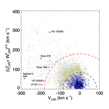
As stated in Section 3.5, Gaia contains radial velocities only for those objects having mag, which omits many of the M dwarfs and all of the L, T, and Y dwarfs within 20 pc. For these objects, we leverage spectroscopic indications of low metallicity to build a list of potential halo members, then we scour the literature for other published radial velocities. These objects are also listed in Table 6.2.2. Many of these lack any radial velocity measurements, so assumed values from 200 to +200 km s-1, in increments of 50 km s-1, were used to calculate a range of possible velocities. These results, shown in Figure 11, suggest that only two of these colder objects – SSSPM J14442019 and WISEA J153429.75104303.3 (aka "The Accident") – are likely to be true halo members.
Figures 10 and 11 taken together suggest that only eight objects (all of them believed to be single) out of 3,589 total in the 20-pc census, or , are halo interlopers. Although this is slightly higher than the percentage of used in Table A of Bensby et al. (2014) based on F and G stars alone, it nevertheless confirms that contamination by halo objects in the 20-pc census is extremely small. Although these objects will still be included in our mass function, any systematic offset imprinted upon their mass estimates can be ignored in subsequent analyses.
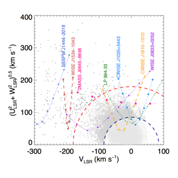
The second concern is difficult to address, as very few low-metallicity objects have had their masses measured via direct methods. The coldest subdwarfs, for instance, have a multiplicity fraction of only (González-Payo et al. 2021); therefore, few such objects exist for dynamical analyses (e.g., Rebassa-Mansergas et al. 2019). Single subdwarfs are obvious targets for lensing-based mass measurements, as their high velocities increase the likelihood of "encounters" with background objects, but accurate whole-sky astrometry is just now advancing to the stage at which such measurements can be predicted and planned for (e.g. Sahu et al. 2020). So, to address this concern, we instead note that only forty-two low-metallicity systems are known within the 20-pc census404040It is worth noting that other low-luminosity, low-metallicity objects are likely to be found within this volume given the fact that parallaxes for both WISEA J153429.75104303.3 ( pc vs. pc; Kirkpatrick et al. 2021b; Meisner et al. 2020a) and CWISE J181005.77101001.2 ( pc vs. 14 - 64 pc; Lodieu et al. 2022; Schneider et al. 2020) placed them far closer to the Sun than original estimates predicted. (Table 6.2.2), which represents only of the total. Thus, if small biases are present in converting a subdwarf’s spectral type, colors, or absolute magnitudes to masses, the bias in the overall 20-pc mass distribution will be negligible.
The above logic on the scarcity of objects also holds for systems with higher metallicity than the Sun. This set of objects has a much smaller range in metallicity than the metal-poor objects above, and there are just a handful of examples. Only the higher-mass stars Hor AB (Fe+0.3), Phe (Fe+0.4), HD 176051 AB (slightly metal strong), and HD 207129 (Fe+0.4) have spectroscopic classifications that fall into this class. Another object, 14 Her, has a supersolar metallicity ([Fe/H] ; Rosenthal et al. 2021) although its listed spectral type in Table 3.1 gives no indication of this. Curiously, even though members of the Hyades Cluster have metallicities that are slightly supersolar ([Fe/H] ; Perryman et al. 1998) and lie, on average, only 47.00.2 pc from the Sun (Lodieu et al. 2019), there are no confirmed Hyads within the 20-pc volume (Gaia Collaboration et al. 2020; Schneider et al. 2022).
6.2.3 Formation process
Because we are interested in objects formed via the star formation process, we need a criterion to distinguish objects that may have formed via alternative formation mechanisms at the lowest masses. When brown dwarfs were first theorized (Kumar 1963; Hayashi & Nakano 1963), they were regarded as direct products of the star formation process – ones that had insufficient mass to sustain prolonged thermonuclear fusion in their cores – and as such represented the lower-mass extension of hydrogen-burning stars themselves. These could be contrasted with another low-mass formation product, planets, that were believed to be formed via a secondary process – from a protoplanetary disk created around a newly formed protostar or brown dwarf. In the early 1960s, there were no known examples of brown dwarfs, and our own Solar System provided the only known examples of planets.
As brown dwarf and exoplanet discoveries began in earnest (see reviews by Kirkpatrick 2005; Winn & Fabrycky 2015), it became clear that nature produces some low-mass products that are difficult to classify as either brown dwarf or exoplanet (e.g., 2MASSWJ 1207334393254b, Chauvin et al. 2004). The earlier definition based on formation was cumbersome to use in practice; unless an object was still in its infancy, its exact formation process would be difficult, if not impossible, to ascertain from observations. As an alternative, Burrows et al. (1997) proposed another theoretically based definition. This alternative uses mass to distinguish between a brown dwarf and an (exo)planet, the dividing line being the somewhat arbitrarily chosen deuterium burning limit, which is for solar metallicity. Somewhat surprisingly, this definition was thereafter widely (though not universally) adopted, in no small part because lower-mass discoveries that earlier would have been called "brown dwarfs" could now be referred to by a more attention-grabbing label of "exoplanet."
This alternative definition, however, came three and a half decades after the original brown dwarf definition, and the concept of planets having being born from a protoplanetary disk (the "nebular hypothesis") had been in the astronomical lexicon for over two centuries (Kant 1755; Laplace 1796). Thus, labeling an object below 13 as a planet often leads to confusion, as some readers – and even researchers – unwittingly apply both definitions in tandem. That is, they assume that a so-named "planet" (by the new, mass-based definition) must have formed via a protoplanetary disk (by the former, formation-based definition). It is difficult to divorce the term "planet" from its formation scenario.
In this paper, one of our goals is to define, or place limits on, the low-mass terminus of star formation. If we were to use the newer definition to include/exclude objects for the mass function analysis, our results would return a terminus of 13, which merely reflects the dividing line chosen by the arbitrary definition. We must, therefore, more carefully consider whether the lowest mass objects in the 20-pc census should be counted as star-formation products or planetary-formation products.
As stated earlier, this definition also lacks easy observational verification. Nonetheless, some methods have been proposed to distinguish formation mechanisms. Öberg et al. (2011) postulated that the carbon to oxygen ratio could be used as one tracer. Planets that formed close to a star would have a solar-like value, like brown dwarfs formed via gravitational collapse, whereas planets formed via accretion of ices beyond the water snowline would have a supersolar value. Those authors acknowledged, however, that measuring an accurate value of is fraught with difficulties (even within our own Solar System), and Calamari et al. (2022) made a similar conclusion based on their analysis of the spectrum of the brown dwarf Gliese 229B. Mollière et al. (2022) show that this simplified picture of the ratio is somewhat more complicated when disk chemical evolution and pebble accretion are taken into account, as well.
Similarly, Morley et al. (2019) showed that the deuterium to hydrogen ratio could be used to distinguish between planets with solar values like Jupiter and Saturn, that formed directly from accretion of gas in the protostellar nebula, and planets with enhanced values like Neptune and Uranus, that presumably formed from accretion of ices. Both and thus have limitations: some objects formed via a protoplanetary disk have values indistinguishable from those of objects born via star formation.
Another promising avenue is the overall metallicity. The giant planets of our Solar System have metal enhancements well above solar values (Wong et al. 2004, Fletcher et al. 2009), and exoplanets are preferentially found around metal-rich host stars (Fischer & Valenti 2005, Wang & Fischer 2015). These facts led Fortney et al. (2008) to propose metallicity-based diagnostics that could distinguish between formation scenarios. Specifically for objects with , a strong 4.5 m CO absorption band along with enhanced - and -band fluxes (from a relative lack of collision-induced absorption by ) are proposed as fingerprints of planet-like formation. However, these diagnostics are likely only useful when comparing populations of objects and not when establishing the formation pathway of individual objects. Metal enrichment is not unique to planet formation, as a collapsing metal-rich cloud can also produce low-mass objects.
Bowler et al. (2023) note that the orientation between the spin axis of the star and the orbital plane of the companion shows promise as another marker of formation, as star-like formation shows a wide range of orientations, whereas planet-like formation prefers values near . This is, however, another marker that can distinguish between populations but cannot be used on an individual object basis.
Schlaufman (2018) demonstrates that companions above lack the tendency to fall primarily around metal-rich hosts that companions below exhibit, which is taken as evidence of core accretion in the lower-mass set. Hoch et al. (2023) likewise find a tentative difference in the trend of values at , which is taken as further evidence that those objects are primarily formed via core accretion, although, as stated above, ratios can be difficult to interpret. Similarly, Ribas & Miralda-Escudé (2007) find differing radial velocity distributions above and below values of . Schlaufman (2018) states that planet-like formation appears to cease above , but not necessarily that star-like formation ceases below . There might still be a range in mass, below , where both processes contribute.
The methods addressed above require data that are so far lacking for most exoplanets or can be used only in comparing populations. Instead, for this paper, we propose a simple scheme whose purpose is merely to exclude objects with a high likelihood of having been formed via a protoplanetary disk while including all others as possible products of star formation. For our scheme, we require at least three bodies in a system because the only parameters available for two-body systems – mass ratio, separation, etc. – can lead to ambiguities when trying to distinguish between formation scenarios.
As an example, Bowler et al. (2020) have used twenty-seven long-period companions labeled as giant planets and brown dwarfs to search for differences in parameters. They find that the population of brown dwarfs has an eccentricity distribution peaking in the range , whereas binaries with mass ratios significantly different from one have an eccentricity distribution peaking closer to . These results indicate that the star formation process tends to create binaries with large eccentricity, and the protoplanetary process tends to form binaries with near-zero eccentricity. To reiterate a point from above, while such trends may be indicative of a population of objects, eccentricity alone cannot be used on an object-by-object basis to distinguish between formation scenarios. The same is true for mass ratio, as doing so can bias our list of potential companions to only the higher mass ones, which could impact our ability to determine star formation’s low-mass cutoff. (Similarly, not selecting on mass ratio can bias our results in the opposite direction, a point we address further in the next section.)
In triple (and higher-order) systems, however, we have other parameters available. Specifically, we note that the hierarchy of empirically observed triple star systems is such that the period of the outer component must be at least five times that of the inner pair (Tokovinin 2004). This is in good agreement with dynamical stability expectations for objects in circular orbits, and the period of the outer component must be even larger than five times the inner one when elliptical orbits are considered (Mardling & Aarseth 2001). Planets that have formed from a protoplanetary disk, on the other hand, can often arrange themselves in stable orbital configurations (e.g., in resonances with one another) that violate the above law. A multi-star system that formed via a collapsing cloud could, presumably, arrange itself in a similar manner if conditions were ideal, but such examples must be exceedingly rare. Therefore, we will use the ratios of orbital periods to identify "exoplanet" systems in the 20-pc census that most likely formed via a protoplanetary disk, and we retain all others for consideration as possible products of star formation.
To this end, Table 6.2.3 lists all of the host objects from Table 3.1 that were labeled as having one or more confirmed exoplanets in the NASA Exoplanet Archive as of 2022 Sep 01414141One additional complication, as stated in Section 3.6.4, is that the NASA Exoplanet Archive uses a dividing line, not , to distinguish between brown dwarfs and exoplanets. Hence, some of the brown dwarfs already listed in Table 3.1 will be double counted; that is, they will have their own separate row in the table while also being listed under the ”#Planets” column. Such objects are flagged in Table 6.2.3.. For systems in which any pair of "exoplanets" violate the , we indicate the innermost pair that violates the rule and exclude all of the planets, thus including only the host star in later analysis. For all others, we have used the NASA Exoplanet Archive to compile their mass measurements. For objects identified only through radial velocity monitoring, we list the values, since the inclination of the system is not known. For other objects – transiting systems, radial velocity systems with astrometric imaging, etc. – we list the actual measured masses. Incorporating these objects in to the stellar mass function analysis will be discussed further in Section 7.
| Name | Coords | # of | NoteaaIndicates whether the "exoplanets" in this system should be considered in our stellar mass function analysis. Notes regarding period violations indicate objects that are excluded, as these are likely objects formed via a protoplanetary disk. In these cases, we list at least one example of component pairs ("b" vs. "c", "c" vs. "d", etc.) that violate the rule. | Mass | ||
|---|---|---|---|---|---|---|
| J2000 | Planets | () | () | Ref. | ||
| (1) | (2) | (3) | (4) | (5) | (6) | (7) |
| Sun | 8 | |||||
| HD 1237 A | 00167951 | 1 | consider | 3.370.09 | 1 | |
| GX And | 0018+4401 | 2bbThe "b" planet is currently considered controversial by the NASA Exoplanet Archive, so only the "c" planet is considered for inclusion in our mass function analysis. | consider | 2 | ||
| 54 Psc AB | 0039+2115 | 1 | consider | 0.2280.011 | 3 | |
| HD 3765 | 0040+4011 | 1 | consider | 4 | ||
| G 268-38 | 00441516 | 2 | consider | 0.02010.0014 | 5 | |
| - | consider | 5 | ||||
| BD+61 195 | 0102+6220 | 1 | consider | 0.01770.0021 | 6 | |
| YZ Cet | 01121659 | 3 | ||||
| CD54 269 | 01145356 | 1 | consider | 0.0260.005 | 7 | |
| HD 7924 | 0121+7642 | 3 | ||||
| And A | 0136+4124 | 3 | consider | 0.68760.0044 | 8 | |
| - | consider | 1.9810.019 | 8 | |||
| - | consider | 4.1320.029 | 8 | |||
| q01 Eri | 01425344 | 1 | consider | 0.940.08 | 9 | |
| Cet | 01441556 | 4 | ||||
| TZ Ari | 0200+1303 | 2ccThis object was reported to have two exoplanets at the time of our original query to the NASA Exoplanet Archive, but it is now believed that the "b" component was a false positive. | consider | 0.210.02 | 10 | |
| HD 13445 A | 02105049 | 1 | consider | 4.420.20 | 11 | |
| BD+47 612 | 0222+4752 | 1 | consider | 12 | ||
| Hor AB | 02425048 | 1ddThis exoplanet, aka HR 810b, has a period from radial velocity variations of 302.82.3d (Stassun et al. 2017) and is presumably the same object listed in Tabe 3.1 as Hor B, the companion giving rise to the 331.7d orbital period in the Gaia DR3 non-single star table. | already included | 2.27±0.25 | 11 | |
| Teegarden’s Star | 0253+1652 | 2 | ||||
| G 245-61 | 0257+7633 | 1 | consider | 0.007330.00063 | 13 | |
| BD17 588 A | 03011635 | 2 | ||||
| CD Cet | 0313+0446 | 1 | consider | 14 | ||
| e Eri | 03194304 | 4 | ||||
| HD 21749 | 03266329 | 2 | ||||
| Eri | 03320927 | 1 | consider | 15 | ||
| HD 22496 | 03354825 | 1 | consider | 16 | ||
| L 372-58 | 03354430 | 3 | ||||
| L 229-91 | 04095322 | 3 | ||||
| Eri A | 04150739 | 1 | consider | 0.02660.0015 | 17 | |
| Ret A | 04165918 | 1 | consider | 1.560.14 | 18 | |
| L 375-2 AB | 04323947 | 2 | ||||
| HD 285968 | 0442+1857 | 1 | consider | 0.02850.0043 | 4 | |
| Wolf 1539 | 0452+0628 | 1 | consider | 0.820.07 | 19 | |
| L 736-30 | 04531746 | 3 | ||||
| LP 656-38 | 05010656 | 2 | consider | 20 | ||
| - | consider | 20 | ||||
| UCAC4 211-005570 | 05054756 | 1eeThis transiting exoplanet, aka TOI-540 b, has no mass measurement. | consider | |||
| Kapteyn’s Star | 05114501 | 1 | consider | 21 | ||
| Men | 05378028 | 3 | consider | 22 | ||
| - | consider | 0.04210.0043 | 23 | |||
| - | consider | 12.21.3 | 22 | |||
| Pic | 05475103 | 2 | excludeffThe inner and outer planets do not violate the rule, but the imaging of this youthful system nonetheless shows the debris disk remaining from protoplanetary formation. | |||
| HD 40307 | 05546001 | 5 | ||||
| Gl 229 A | 06102151 | 2 | ||||
| HD 260655 | 0637+1733 | 2 | ||||
| HD 265866 | 0654+3316 | 1 | consider | 0.01260.0013 | 24 | |
| BD+05 1668 | 0727+0513 | 2 | ||||
| Gem | 0745+2801 | 1 | consider | 2.300.45 | 25 | |
| L 34-26 | 07497642 | 1ggThis "exoplanet" is the T dwarf WISEPA J075108.79763449.6, already included as its own row in Table 3.1. | already included | |||
| CD24 6144 | 07542518 | 2 | consider | 0.0250.005 | 26 | |
| - | consider | 0.1520.023 | 26 | |||
| L 97-3 A | 08066618 | 1hhThis "exoplanet" is the Y dwarf L 97-3 B (sometimes referred to as WD 0806661 B), already included as its own row in Table 3.1. | already included | |||
| L 98-59 | 08186818 | 4 | ||||
| HD 69830 | 08181237 | 3 | ||||
| L 675-81 | 08402327 | 2 | consider | 1.7530.058 | 26 | |
| - | consider | 1.6440.060 | 26 | |||
| G 234-45 | 0841+5929 | 2 | consider | 27 | ||
| - | consider | 0.200.01 | 27 | |||
| Cnc A | 0852+2819 | 5 | ||||
| HD 79211 | 0914+5241 | 1 | consider | 0.03340.0038 | 28 | |
| L 678-39 | 09362139 | 3 | ||||
| CD45 5378 | 09444546 | 1 | consider | 0.001720.00025 | 29 | |
| HD 85512 | 09514330 | 1 | consider | 0.0110.002 | 30 | |
| BD+63 869 | 0956+6247 | 1 | consider | 0.07210.0088 | 26 | |
| BD+48 1829 | 1002+4805 | 1 | consider | 31 | ||
| HD 87883 | 1008+3414 | 1 | consider | 22 | ||
| L 320-124 | 10144709 | 2 | consider | 0.005220.00072 | 32 | |
| - | consider | 0.00830.0014 | 32 | |||
| BD+01 2447 | 1028+0050 | 1 | consider | 0.005380.00076 | 33 | |
| 47 UMa | 1059+4025 | 3 | ||||
| Lalande 21185 | 1103+3558 | 2 | consider | 34 | ||
| - | consider | 34 | ||||
| BD18 3106 | 11071917 | 2 | ||||
| HD 97101 A | 1111+3026 | 2 | consider | 35 | ||
| - | consider | 35 | ||||
| HD 304043 | 11165732 | 1 | consider | 0.03480.0035 | 7 | |
| 83 Leo B | 1126+0300 | 1 | consider | 0.0700.050 | 11 | |
| CD31 9113 | 11353232 | 3 | ||||
| Ross 1003 | 1141+4245 | 2 | consider | 36 | ||
| - | consider | 36 | ||||
| Ross 905 | 1142+2642 | 1 | consider | 0.0700.007 | 37 | |
| HD 102365 A | 11464030 | 1 | consider | 0.0500.008 | 38 | |
| Ross 128 | 1147+0048 | 1 | consider | 0.004400.00066 | 39 | |
| HD 238090 | 1212+5429 | 1 | consider | 24 | ||
| Wolf 433 | 1238+1141 | 1 | consider | 0.04150.0053 | 26 | |
| Wolf 437 | 1247+0945 | 1 | consider | 40 | ||
| BD+13 2618 AB | 1300+1222 | 1iiThis "exoplanet" is the T dwarf ULAS J130041.74+122114.7, already included as its own row in Table 3.1. | already included | |||
| HD 113538 | 13045226 | 2 | ||||
| e Vir | 1316+0925 | 1jjThis "exoplanet" is the late-T/early-Y dwarf e Vir Ab, already included as its own row in Table 3.1. | already included | |||
| 61 Vir | 13181818 | 3 | ||||
| Ross 1020 | 1322+2428 | 1 | consider | 0.0250.002 | 41 | |
| 70 Vir | 1328+1346 | 1 | consider | 7.4160.057 | 42 | |
| BD+11 2576 | 1329+1022 | 1 | consider | 0.0160.003 | 43 | |
| Boo A | 1347+1727 | 1 | consider | 4.320.04 | 44 | |
| HD 122303 | 14010239 | 1 | consider | 45 | ||
| Proxima Centauri | 14296240 | 1 | consider | 0.003370.00019 | 46 | |
| HD 128311 | 1436+0944 | 2 | ||||
| BD07 4003 | 15190743 | 3 | ||||
| Lup | 15214819 | 3 | ||||
| Ross 508 | 1523+1727 | 1 | consider | 0.01260.0017 | 47 | |
| Ser | 1546+0721 | 1 | consider | 0.04290.0046 | 4 | |
| G 180-18 | 1558+3524 | 2 | consider | 0.00550.0014 | 48 | |
| - | consider | 0.01800.0030 | 48 | |||
| CrB | 1601+3318 | 2kkThis assumes that the exoplanet candidate CrB b is real. | ||||
| GJ 3942 | 1609+5256 | 1 | consider | 0.02250.0019 | 49 | |
| 14 Her | 1610+4349 | 2 | consider | 22 | ||
| - | consider | 22 | ||||
| LP 804-27 | 16121852 | 1 | consider | 2.1 | 50 | |
| HD 147379 | 1616+6714 | 1 | consider | 12 | ||
| HD 147513 | 16243911 | 1 | consider | 1.21 | 51 | |
| G 202-48 | 1625+5418 | 1 | consider | 0.00890.0016 | 52 | |
| BD12 4523 | 16301239 | 3 | ||||
| BD+25 3173 | 1658+2544 | 1 | consider | 0.3280.032 | 53 | |
| HD 154345 | 1702+4704 | 1 | consider | 0.820.07 | 11 | |
| HD 154088 | 17042834 | 1 | consider | 0.0210.003 | 54 | |
| G 139-21 | 1715+0457 | 1 | consider | 0.02570.0014 | 55 | |
| BD+11 3149 | 1716+1103 | 2 | consider | 0.007770.00085 | 56 | |
| - | consider | 56 | ||||
| HD 156384 C | 17183459 | 5 | ||||
| CD46 11540 | 17284653 | 1 | consider | 0.035 | 57 | |
| CD51 10924 | 17305138 | 4 | consider | 0.01200.0010 | 22 | |
| - | consider | 22 | ||||
| - | consider | 22 | ||||
| - | already includedllIn Table 3.1, we label the object causing the Gaia DR3 acceleration (from the non-single star list) as CD51 10924 B. For the purposes of accounting, we will equate that object with this one, GJ 676 A c. | 13.431.1 | 22 | |||
| G 226-66 | 1735+6140 | 1 | consider | 58 | ||
| BD+68 946 | 1736+6820 | 2 | consider | 0.05410.0031 | 26 | |
| - | consider | 0.0500.013 | 26 | |||
| CD44 11909 | 17374419 | 2 | ||||
| BD+18 3421 | 1737+1835 | 1 | consider | 0.02080.0014 | 59 | |
| Ara | 17445150 | 4 | ||||
| BD+45 2743 A | 1835+4544 | 1 | consider | 0.04290.0025 | 60 | |
| HD 176029 | 1858+0554 | 1 | consider | 61 | ||
| HD 177565 | 19063748 | 1 | consider | 62 | ||
| HD 180617 | 1916+0510 | 1 | consider | 0.03840.0033 | 59 | |
| HD 189733 | 2000+2242 | 1 | consider | 1.130.08 | 11 | |
| HD 190007 | 2002+0319 | 1 | consider | 0.05180.0052 | 59 | |
| HD 190360 | 2003+2953 | 2 | consider | 0.06000.0076 | 63 | |
| - | consider | 1.80.2 | 64 | |||
| HD 189567 | 20056719 | 2 | ||||
| HD 192263 | 20130052 | 1 | consider | 0.560.05 | 11 | |
| HD 192310 | 20152701 | 2 | consider | 0.05320.0028 | 30 | |
| - | consider | 0.0760.016 | 30 | |||
| AU Mic | 20453120 | 2 | ||||
| LSPM J2116+0234 | 2116+0234 | 1 | consider | 65 | ||
| LSPM J2122+2255 | 2122+2255 | 1 | consider | 0.330.02 | 10 | |
| HD 204961 | 21334900 | 2mmThe "c" planet is currently considered controversial by the NASA Exoplanet Archive, so only the "b" planet is considered for inclusion in our mass function analysis. | consider | 0.680.09 | 66 | |
| HN Peg AB | 2144+1446 | 1nnThis "exoplanet" is the T dwarf HN Peg B, already included as its own row in Table 3.1. | already included | |||
| G 264-12 | 2146+6648 | 2 | ||||
| Ind A | 22035647 | 1 | consider | 67 | ||
| BD05 5715 | 22090438 | 2 | ||||
| L 788-37 | 22131741 | 1 | consider | 0.0230.002 | 41 | |
| HD 211970 | 22225433 | 1 | consider | 0.04090.0079 | 68 | |
| L 119-213 | 22416910 | 1 | considerooThis object has no mass determination. | |||
| HD 216520 | 2247+8341 | 2 | ||||
| BD15 6290 AB | 22531415 | 4 | ||||
| 51 Peg | 2257+2046 | 1 | consider | 0.4720.039 | 18 | |
| HD 217987 | 23053551 | 2 | ||||
| TRAPPIST-1 | 23060502 | 7 | ||||
| HD 219134 | 2313+5710 | 6 | ||||
| Cep AB | 2339+7737 | 1 | consider | 1.850.16 | 69 |
References. — References for the mass measurements: 1 = Naef et al. (2001), 2 = Pinamonti et al. (2018), 3 = Wittenmyer et al. (2019), 4 = Rosenthal et al. (2021), 5 = Lillo-Box et al. (2020), 6 = Perger et al. (2019), 7 = Feng et al. (2020), 8 = Curiel et al. (2011), 9 = Marmier et al. (2013), 10 = Quirrenbach et al. (2022), 11 = Stassun et al. (2017), 12 = Hobson et al. (2018), 13 = Soto et al. (2021), 14 = Bauer et al. (2020), 15 = Llop-Sayson et al. (2021), 16 = Lillo-Box et al. (2021), 17 = Ma et al. (2018), 18 = Butler et al. (2006), 19 = Howard et al. (2010), 20 = Astudillo-Defru et al. (2017), 21 = Anglada-Escude et al. (2014), 22 = Feng et al. (2022), 23 = Hatzes et al. (2022), 24 = Stock et al. (2020), 25 = Hatzes et al. (2006), 26 = Feng et al. (2020b), 27 = Lopez-Santiago et al. (2020), 28 = DiTomasso et al. (2023), 29 = Lam et al. (2021), 30 = Pepe et al. (2011), 31 = Hobson et al. (2019), 32 = Bonfils et al. (2018), 33 = Amado et al. (2021), 34 = Hurt et al. (2022), 35 = Dedrick et al. (2021), 36 = Trifonov et al. (2018), 37 = Maciejewski et al. (2014), 38 = Tinney et al. (2011), 39 = Bonfils et al. (2018b), 40 = Trifonov et al. (2021), 41 = Luque et al. (2018), 42 = Luhn et al. (2019), 43 = Damasso et al. (2022), 44 = Borsa et al. (2015), 45 = Suárez Mascareño et al. (2017), 46 = Faria et al. (2022), 47 = Harakawa et al. (2022), 48 = Beard et al. (2022), 49 = Perger et al. (2017), 50 = Apps et al. (2010), 51 = Mayor et al. (2004), 52 = Suárez Mascareño et al. (2017b), 53 = Johnson et al. (2010), 54 = Unger et al. (2021), 55 = Cloutier et al. (2021), 56 = Affer et al. (2016), 57 = Bonfils et al. (2007), 58 = Pinamonti et al. (2019), 59 = Burt et al. (2021), 60 = González-Álvarez et al. (2021), 61 = Toledo-Padrón et al. (2021), 62 = Feng et al. (2017), 63 = Wright et al. (2009), 64 = Feng et al. (2021), 65 = Lalitha et al. (2019), 66 = Wittenmyer et al. (2014), 67 = Feng et al. (2019), 68 = Feng et al. (2019b), 69 = Endl et al. (2011).
6.3 Objects on the main sequence
Main sequence objects with directly measured masses can be used to calibrate relations of mass vs. absolute magnitude or mass vs. spectral type. Studies have shown that the relation with the smallest intrinsic scatter for K and M dwarfs is the one using absolute -band magnitude (Delfosse et al. 2000). The fact that the -band relation shows the least scatter across the optical to near-infrared range is also predicted by model atmospheres, as this is the wavelength regime where competing physical effects modulated by metallicity variations largely cancel one another (Delfosse et al. 2000; Mann et al. 2019). More (and improved) dynamical mass measurements of binary stars424242In reality, the total mass of the binary system was used, rather than the masses of the individual components, the latter of which are not generally known. The resulting relation is nonetheless applicable to individual objects, as sections 7.3 and 7.4 of Mann et al. (2019) discuss in detail. See in particular their figure 15, which shows a direct comparison between directly measured individual masses and the resulting mass- relation. along with improved Gaia parallaxes have enabled Mann et al. (2019) to construct a mass vs. relation that results in estimated masses with only 2-3% uncertainty. Specifically, is used because 2MASS provides all-sky coverage at this band. We use the Mann et al. (2019) mass- relation (their equation 2) over the range , roughly corresponding to spectral types from early-M to late-M434343Their relation covers the range from mag down to a spectral type of L1. However, the bright end of the relation is poorly constrained, so for these objects we defer to the TIC mass estimates (see the next paragraph). At the faint end, we use the effective temperature analysis for objects cooler than M9.5, as further described in Section 7.1.. These estimates and their propagated uncertainties are listed in columns "EstMassMKs" and "EstMassMKsErr" of Table 3.1.
For other main sequence stars, we can use the methodology employed by Stassun et al. (2019). Using 20,000 (non-reddened) stars within 100 pc of the Sun with spectroscopically determined effective temperatures, they established a relation between and color. This is then mated with the results of Torres et al. (2010) that relate to mass for stars with dynamically measured masses (Stassun et al. 2018b). This gives mass estimates with uncertainties of (Stassun et al. 2019). We take mass estimates and their uncertainties directly from the revised TESS Input Catalog (TIC; Stassun et al. 2019) for stars in our Table 3.1. These values are listed in columns "EstMassTIC" and "EstMassTICErr". We note, however, that the Stassun et al. (2019) prescription for stars with K (see their appendix A.1 along with Muirhead et al. 2018) followed a different methodology. For these objects, masses were estimated using magnitudes, Gaia DR2 parallaxes, and the Mann et al. (2019) mass-vs.- relation.
Some main sequence stars lack both magnitudes and an entry in the TESS Input Catalog. For these, we resort to two other estimation methods. The first is the mass vs. relation. Chontos et al. (2021) took a list of well-studied late-K and M dwarfs (tables 5-7 from Mann et al. 2015) and refined their mass estimates using more precise Gaia DR3 parallaxes and the Mann et al. (2019) mass-vs.- relation from above. They derived a relation between this estimated mass and the absolute G-band magnitude. However, the coefficients in Chontos et al. (2021) are published with insufficient accuracy to re-create the relation show in their figure 7, so we have re-derived them here. Our methodology is identical to theirs except that we exclude the sdM3 object L 750-42 (Gizis 1997) and do not incorporate a dependence on metallicity because the metallicity has not been measured for most of the M dwarfs within 20 pc. Using a functional form of
| (18) |
where is the G-band absolute magnitude in magnitudes and Mass is in units of , we find best-fit coefficients of , , , , and . Our fit is illustrated in Figure 12. The relation is valid from (spectral types from K7 to M8). For uncertainty propagation, we adopt the Chontos et al. (2021) practice of a 2.2% uncertainty added in quadrature to the 3% uncertainty inherent to the Mann et al. (2019) relation. This mass- relation is particularly useful for estimating masses of individual components of close double systems that are currently resolved only by Gaia. In Table 3.1 we provide columns labeled "EstMassMG" and "EstMassMGErr" listing mass estimates for all objects for which these -based estimates can be computed.
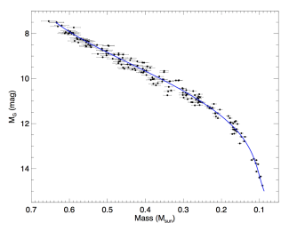
The second alternative estimation method is StarHorse (Anders et al. 2022), which uses Gaia EDR3 data cross-matched to photometry from Pan-STARRS1, SkyMapper, 2MASS, and AllWISE to estimate stellar parameters from stellar isochrones (from PARSEC 1.2S; Marigo et al. 2017) providing the closest match. When Anders et al. (2022) mass estimates are available, these are listed in columns "EstMassSH" and "EstMassSHErr" of Table 3.1. These published mass uncertainties can be anomalously low compared to the other estimates discussed in this section because they pertain only to the internal model errors and do not include the systematic component coming from a model-to-truth comparison.
Figure 13 shows the four estimation techniques compared to each other. The top three panels show the intercomparisons between the TESS Input Catalog estimates, the estimates, and the estimates. As these are all based on the same underlying mass vs. relation of Mann et al. (2019), the correspondence is generally excellent. (In fact, the correspondence between the TESS Input Catalog estimates and estimates from our technique are nearly perfect, differing only in the Gaia data release from which the parallax values were obtained.) The only deviation is for masses greater than in the comparison between the TESS Input Catalog values and those derived from , where the difference can be as large as 13%.
The bottom three panels of Figure 13 show small systematics between the three estimation techniques above and StarHorse. As stated above, masses from StarHorse are based on theoretical models, so such systematics might be expected between theory and observation. At masses of , StarHorse tends to overpredict (by 10%) the mass relative to the other techniques, and at smaller masses may significantly underpredict (by 35%). At masses near , a small underprediction (by 5%) relative to the TESS Input Catalog becomes an overprediction (by 5%) relative to masses from the relation. At masses closer to , StarHorse leads to underpredictions (by 10%) relative to estimates from the TESS Input Catalog.
Given that systematic offsets of up to 15% are seen even between the sets with empirical underpinnings, we are reluctant to apply corrections to offsets smaller than this value. The only exception to this is the 35% offset seen for StarHorse estimates below StarHorse values of . In this case, rather than applying an offset, we will simply not use any StarHorse estimates below .
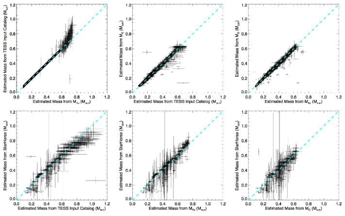
7 Further Analysis
For each individual object ("#CompsOnThisRow" = 1) in Table 3.1, we have adopted a mass and its uncertainty. These are listed in columns "AdoptedInitialMass" and "AdoptedInitialMassErr" along with an additional column, "AdoptedInitialMassNote", indicating the origin of the data from elsewhere in the table. These are labeled with the term "Initial" as a reminder that for white dwarfs, we need their initial masses on the main sequence; for all other objects, their current masses are assumed identical to their initial masses. The codes for "AdoptedInitialMassNote" are as follows, listed in their order of selection:
-
•
wd IFMR, wd low, wd ultra-low, or wd conjecture: The initial mass and its uncertainty have been computed via the initial-to-final mass relation or other means (see Table 6.1.1), if this object is a white dwarf.
-
•
measured: Directly measured mass values from "Mass" and "MassErr" are used. The methodology used and its reference are listed in columns "MassMethod" and "MassRef". (For L, T, and Y dwarfs, directly measured masses are not retained because these are estimated in bulk through statistical means; see the Teff bullet, below.)
-
•
M_Ks: The mass and its uncertainty from the Mann et al. (2019) relation ("EstMassMKs" and "EstMassMKsErr") are used.
-
•
TIC: The mass and its uncertainty from the TESS Input Catalog (Stassun et al. 2019; "EstMassTIC" and "EstMassTICErr") are used.
-
•
M_G: The mass and its uncertainty from the relation of Equation 18 ("EstMassMG" and "EstMassMGErr") are used.
- •
-
•
literature: The mass and its uncertainty are taken from columns "EstMassLit" and "EstMassLitErr", the mass estimation method and reference for which are listed in "EstMassLitMethod" and "EstMassLitRef". (Literature values can supersede other values above if the object is listed as a giant or subgiant in Table 6.1.2.)
-
•
see GeneralNotes: For objects with this code, the mass and its uncertainty were computed by us, as detailed in the "GeneralNotes" column of the table.
-
•
Teff: For objects of type L, T, or Y, individual masses are not computed. These are handled statistically via the distribution of values and their uncertainties ("Teff" and "Teff_unc"), as described in detail below.
For cases in which literature values did not list a mass uncertainty, a value of 10% is arbitrarily assumed. The quoted StarHorse uncertainty is also replaced with a 10% uncertainty, based on the under- and over-predictions noted when comparing StarHorse values to other estimates (see discussion at end of Section 6.3), unless the quoted StarHorse internal uncertainty is already larger, in which case we retain the published value.
For cases where only a miscellaneous magnitude or delta magnitude of a companion were available, it is instructive to estimate a spectral type for the object in order to estimate its mass. Figure 14 shows a comparison between masses and measured spectral types for those Table 3.1 objects having mass estimates (or direct measures) from one of the other methods. The piecewise fit shown in the figure is the one we use to translate a dwarf spectral type estimate into a mass estimate. Other per-object details can be found in the General Notes column of Table 3.1.
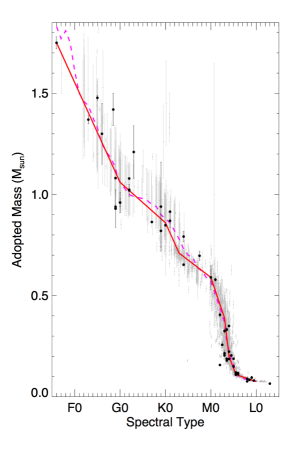
| Spectral Type | Spectral Index | Mass () |
|---|---|---|
| (1) | (2) | (3) |
| A6 | 6.0 | 1.75 |
| G0 | 20.0 | 1.06 |
| K0 | 30.0 | 0.86 |
| K3 | 33.0 | 0.71 |
| M0 | 40.0 | 0.59 |
| M3 | 43.0 | 0.39 |
| M4 | 44.0 | 0.20 |
| M5.5 | 45.5 | 0.11 |
| L0 | 50.0 | 0.075 |
Note. — Each row in this table represents an inflection point in the red, piecewise fit of Figure 14.
7.1 Analysis of brown dwarfs
We use the methodology adopted by Kirkpatrick et al. (2019, 2021a) and Raghu et al. (submitted) to determine the mass function for L, T, and Y dwarfs, most of which are brown dwarfs lacking any color (or spectral type or absolute magnitude) to mass correlation. Specifically, the mass function for these objects is determined by comparing the distribution of present-day temperatures to predicted temperature distributions. Predictions are drawn from a grid of models with varying mass functions, birthrates, and low-mass cutoffs. For each point in the grid, we build a predicted mass/age distribution that is then passed through a set of evolutionary models to predict the current-day distribution. Using this grid of predictions allows us to find the combination of mass function, birthrate, and cutoff mass that best fits the observed temperature distribution.
For the empirical distribution, we estimate the value for each L, T, or Y dwarf (see Table 16 in this paper and table 11 of Kirkpatrick et al. 2021a) and then calculate space densities as a function of . To compute space densities, we need to determine the distances at which our brown dwarf subsamples are truly complete, as the coldest Y dwarfs are so intrinsically dim that we are unable to push their completeness to the 20-pc limit targeted in this paper. As described in Kirkpatrick et al. (2021a), we determine completeness via the test (Schmidt 1968) using 150K bins and computing at half-parsec steps within each bin. The computation starts with the first half-parsec step falling just larger than the distance of the bin’s nearest object and advances in distance out to pc. These results are shown in Figure 15.
A comparison of this figure to figure 23 of Kirkpatrick et al. (2021a) shows that, despite the many new discoveries (and many fewer retractions) noted in Table 16, each 150K bin has the same completeness limit as before. As one example, consider the bin with the largest change, 600-750K. In both Kirkpatrick et al. (2021a) and here, this bin is complete out to 20 pc, but the number of objects has nonetheless increased from eighty-three in Kirkpatrick et al. (2021a) to ninety-eight in this paper; see also Table 21. (The test is only as robust as the Poisson statistics allow, which is why both sets of numbers were deemed to be complete.) As another example, the number of objects interior to the completeness limit of 15.0 pc in the 450-600K bin has increased from fifty-three to fifty-six.
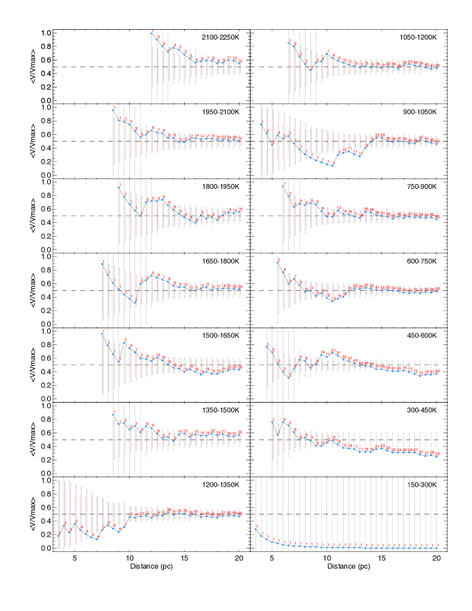
As noted in Kirkpatrick et al. (2021a), the test does not check for inhomogeneities in surface area, the most likely cause of which would be confusion along the Galactic plane that hinders our ability to find nearby brown dwarfs. Do the increased densities now reported in this paper indicate that these corrections can be reduced or dropped altogether?
Figure 16 shows the positions in Galactic coordinates of all 583 L, T and Y dwarfs in the 20-pc census. As was done in Kirkpatrick et al. (2021a), we divide the sky into two zones: a zone along the Galactic plane () and another () well outside of the plane. This value of was chosen so that the non-plane zone contains exactly three times the area of the plane zone. If there is no incompleteness along the Galactic plane, then the ratio of non-plane to plane objects should be three. For the volume-complete portions of our 20-pc census, we find that this ratio is for L dwarfs, for T dwarfs, and for Y dwarfs, suggesting that the Galactic plane does not introduce any significant incompleteness (%) for L dwarfs but does still impede the discovery of fainter T and Y dwarfs. In contrast, Kirkpatrick et al. (2021a) derived ratios of , , and for the L, T and Y dwarf samples, respectively.
Incompleteness along the Galactic plane has improved in the current 20-pc census for the L and T dwarfs. For the Y dwarfs, the view is complicated by smaller number statistics. Taking the non-plane numbers of Y dwarfs as truth, then the number of plane Y dwarfs in the current sample should be , which is different from the value of 4 actually found. The same computation for the Kirkpatrick et al. (2021a) numbers gives a number of plane Y dwarfs that was only different. Hence, the under-density of Y dwarfs in the plane is now significantly worse, due to the fact that all new discoveries of Y dwarfs within the volume have been found outside of the plane zone.
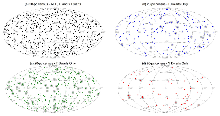
| Teff | Complete- | Raw | Corr. | Adjusted | Adopted |
|---|---|---|---|---|---|
| Bin | ness Limit | No. of | FactoraaAs the bins from 1050 to 1350K encompass both L and T dwarfs (see figure 22b of Kirkpatrick et al. 2021a), we average the correction factor for L dwarfs (1.00) and T dwarfs (1.06). | No. of | Space DensitybbThis value is computed via the equations and where . |
| (K) | (pc) | Objects | Objects | (10-3 pc-3) | |
| (1) | (2) | (3) | (4) | (5) | (6) |
| 2100-2250 | 20.0ccThis bin is complete only for its L dwarf complement. Since late-M dwarfs are also expected to populate this bin, the derived space density is considered to be a lower limit. | 12 | 1.00 | 13.32.8 | 0.36 |
| 1950-2100 | 20.0 | 27 | 1.00 | 21.23.4 | 0.810.19 |
| 1800-1950 | 20.0 | 16 | 1.00 | 21.13.6 | 0.480.16 |
| 1650-1800 | 20.0 | 24 | 1.00 | 23.03.8 | 0.720.19 |
| 1500-1650 | 20.0 | 26 | 1.00 | 25.13.9 | 0.780.19 |
| 1350-1500 | 20.0 | 35 | 1.00 | 34.24.7 | 1.040.23 |
| 1200-1350 | 20.0 | 69 | 1.03 | 54.65.4 | 2.120.30 |
| 1050-1200 | 20.0 | 45 | 1.03 | 44.35.3 | 1.380.26 |
| 900-1050 | 20.0 | 50 | 1.06 | 43.55.0 | 1.580.27 |
| 750-900 | 20.0 | 63 | 1.06 | 54.95.6 | 1.990.31 |
| 600-750 | 20.0 | 98 | 1.06 | 77.66.3 | 3.100.37 |
| 450-600 | 15.0 | 56 | 1.06 | 44.84.9 | 4.200.67 |
| 300-450 | 11.0 | 15 | 1.15 | 17.23.0 | 3.09ddThis temperature bin is not fully populated, as WISE sensitivity limits cannot probe to the quoted completeness distance for Y dwarfs below K. |
| 150-300 | 1 |
L dwarfs no longer show an underdensity in the plane, so no correction is needed for our derived L dwarf space densities. T dwarf space densities should, however, be multiplied by 1.06 to account for the observed incompleteness. The Y dwarf incompleteness is harder to assess given the small number of Y dwarfs in the plane, but the raw numbers suggest a conservative correction factor of 1.15, slightly larger than the 1.13 factor adopted by Kirkpatrick et al. (2021a). These factors are listed in Table 21.
The final step in measuring the space densities of L, T, and Y dwarfs is assessing their measurement uncertainties. For this we adopt the same methodology used in Kirkpatrick et al. (2021a). To summarize, our confidence in assigning an object to a bin is directly related to the measurement uncertainty on , which is often comparable to the bin size itself. To estimate our confidence in the numbers of objects in each bin, we have run simulations with 10,000 Monte Carlo realizations wherein we take the uncertainty in and multiply it by a random value generated from a normal distribution having a mean of 0 and a standard deviation of 1. For each simulation, this uncertainty is added onto the measured value and the object (re-)assigned to the appropriate bin. The computed means and standard deviations across all 10,000 realizations are given in column 5 of Table 21. We use only these computed standard deviations in our adopted space densities, but not the adjusted means. As further explained in Kirkpatrick et al. (2021a), the reason for this is that the number of objects is not preserved across the Monte Carlo simulations because some objects scatter into the hotter, incomplete bin at 2100-2250K and are lost, while objects at the other temperature extreme may be lost because they fall outside the completeness limit of the colder bin. This last loss is one-sided, however, as any colder objects scattering into the warmer bin would be necessarily retained. Hence, we compute our adopted space densities using the raw number counts, but including the uncertainties derived from our simulations, as shown in the footnote of Table 21. These densities are graphically illustrated in Figure 17.
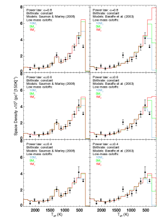
The measured space densities can now be compared to the simulated distributions (Raghu et al., submitted) to infer the form of the mass function at this low-mass end. Following on the results of Kirkpatrick et al. (2021a), which showed the best match to be a power law, , with , Raghu et al. (submitted) assume power-law functional forms with values between 0.3 and 0.8 and, like Kirkpatrick et al. (2021a), choose low-mass cutoffs of 1, 5, and 10 . Unlike Kirkpatrick et al. (2021a), however, they vary the birthrate to include not only a constant birthrate over the lifetime of the Milky Way, but also consider two other birthrates – called inside-out and late-burst – from Johnson et al. (2021) that are constrained by new results from Gaia. The inside-out birthrate represents a declining birthrate over the 10 Gyr lifetime of the Galactic disk, and the late-burst birthrate is identical to the inside-out form, except with an abrupt increase (by a factor of 3) in star formation 3-5 Gyr ago.
Evolutionary models are used to infer the current value of each simulated object (using its mass and age). Raghu et al. (submitted) expand the model set used in Kirkpatrick et al. (2021a) by including the newer Marley et al. (2021) predictions and show (again) that the only evolutionary models able to fit the bump in the L/T transition in the distribution are those of Saumon & Marley (2008).
It has been shown in Kirkpatrick et al. (2021a) and Raghu et al. (submitted) that the low-mass cutoff has little effect on the shape of the mass function at values above 450K, where our fitting is taking place. Therefore, we consider each + birthrate pair and compute the median of the least squared values for the simulations across all three cutoff masses. The minimum is achieved for and a constant birthrate, identical to the findings in Kirkpatrick et al. (2021a). The second best fit is achieved for and a constant birthrate. The third best fit is a tie among the + constant, the + late-burst, and + late-burst models. Use of either the late-burst or inside-out birthrates results in a slightly reduced because those birthrates create a small overabundance, relative to the constant birthrate models, of older brown dwarfs that have already cooled to cooler temperatures.
In Figure 17, we show the fits for three values of (0.4, 0.6, and 0.8) all paired with a constant birthrate. The panels in the left column of the figure show that the model with a constant birthrate and using the Saumon & Marley (2008) evolutionary models is an excellent representation of the empirical data. Can any new conclusions be gleaned regarding the low-mass cutoff? As figure 4 of Raghu et al. (submitted) illustrates, the Saumon & Marley (2008) models are incomplete below masses of 0.015 (16), so they are a poor choice for determining what the low-mass cutoff might be. Instead, we revert back to the Baraffe et al. (2003) models, that are complete down to 5. As the rightmost panels in Figure 17 illustrate, our ability to distinguish between low-mass cutoffs depends on measuring accurate space densities below 450K. Using the 20-pc census to say confidently that star formation’s terminus is below 10 or even 5 depends on surveying the sky more deeply at the wavelengths of these objects’ peak emission and obtaining the necessary astrometry to measure accurate distances. As the simulations using the Baraffe et al. (2003) models show, measuring an accurate space density for the 300-450K bin will allow us to distinguish between the cutoff masses, and even a few more objects discovered in the 150-300K bin, which currently has only the 250K Y dwarf WISE J085510.83071442.5 in it, will provide even tighter constraints.
Have some of these ultra-low mass products of star formation already been identified, and are they masquerading in the literature as exoplanet discoveries to higher mass objects? We use our analysis in Table 6.2.3 to see first if the omission of these objects has biased our derivation of the brown dwarf mass function above. With the exception of the two objects (the companions to UCAC4 211-005570 and L 119-213) lacking mass estimates, we take all objects labeled as "consider" in column 4 of Table 6.2.3 and estimated their contribution to the overall mass function. For objects with measurements only, we pull a random number from a distribution of values uniformly distributed between 0 and 1 and multiply that number by 90 degrees to assign each an inclination, which we then use to assign an actual mass value. For all masses, whether or not they are true masses or adjusted measurements, we then pull a random number from a normal distribution with a mean of 0 and standard deviation of 1 and multiply that number by the uncertainty, which we then add back to the mass value. We perform this methodology over 10,000 Monte Carlo iterations and find the mean and standard deviation of the resulting space density, binned over 0.001- mass intervals, as illustrated in Figure 18.
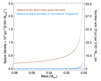
This figure shows that our derived space density of brown dwarfs, (which we find to be in units of # , with in units of ; see Section 8), overwhelms the space density above where our fitting took place. So, the omission of these objects has no impact on our derivation. However, the second question is whether any of these objects could be products of star formation itself rather than the secondary by-products of a proto-planetary disk. That question cannot be answered from this diagram, but it is a statistical certainty that at least a few of the objects on the high-mass tail of this distribution are star formation products. One striking result from Figure 18, however, is the high space density of objects in the lowest mass bin, given that the census of such low-mass objects, whether resulting from star formation or proto-planetary disks, is still woefully incomplete. There is clearly no shortage of ultra-low mass objects in the Milky Way.
7.2 Combined stellar and brown dwarf space densities
With the brown dwarf portion of the mass function now fitted, we can combine the stellar and brown dwarf portions to determine the shape of the overall mass function.
First we take the number counts across the stellar regime and perform a similar Monte Carlo analysis as was done on the brown dwarfs. Specifically, for each object we pull a random number from a normal distribution with a mean of 0 and a standard deviation of 1. We then multiply the mass measurement uncertainty by the random number and add that back to the mass value to get a true mass. We do this for each of the stars in our sample, and repeat the process 10,000 times to simulate 10,000 possible histograms. We then compute the mean value in each histogram bin along with its standard deviation. Because the 20-pc volume around the Sun is just one of many such volumes that can be taken as a sample of the Milky Way, we add the Poisson uncertainty and the standard deviation from above in quadrature to provide the final uncertainty per bin. (This parallels the brown dwarf space density analysis of Table 21.)
We can now append the substellar contribution onto this stellar distribution. To do this, we look at the predictions from the best fit Raghu et al. (submitted) model to the brown dwarf distribution from above, which is the power law with a constant birthrate function and passed through the Saumon & Marley (2008) evolutionary models. We also choose a 0.005 () cutoff to parallel the more detailed cutoff analysis from Kirkpatrick et al. (2021a). This simulation gives the predicted mass distributions shown in Figure 19. Each histogram is scaled so that the total number of objects in each histogram matches the raw numbers of objects per bin listed in Table 21. As one example, the 27 objects in the 1950-2100K bin are predicted to fall almost exclusively in the 0.075-0.080 bin, and these predictions suggest that our 27 objects be apportioned as 20.5 objects in the 0.075-0.080 bin, 2.0 objects in the 0.070-0.075 bin, 1.0 object in the 0.065-0.070 bin, and fractional numbers of objects in bins of lower mass. As another example, the 63 objects in the 750-900K bin are spread over a wide range of masses from 0.005-0.060 and are apportioned as 2.6 objects in the 0.055-0.060 bin, 10.8 objects in the 0.050-0.055 bin, 12.3 objects in the 0.045-0.050 bin, 10.7 objects in the 0.040-0.045 bin, 8.3 objects in the 0.035-0.040 bin, etc.
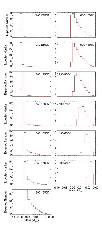
We take the apportionment across all thirteen temperature bins and tally the results in each of the 0.005-wide mass bins, after also applying the factor (corr in Table 21) to correct for losses of objects along the Galactic plane and extrapolating the numbers to the full 20-pc volume if that temperature bin was not complete to 20 pc. For example, the raw number counts in the 450-600K bin shown in both Table 21 and Figure 19 were multiplied by the 1.06 correction factor then multiplied by to extrapolate to the full volume. In Table 21, we find that our lowest temperature bin with a space density measurement, 300-450K, is considered to be incomplete, and the mass distribution for that bin in Figure 19 suggests that that bin’s objects fall exclusively below 0.025. Therefore we consider any space density measurements below this mass value to be lower limits only.
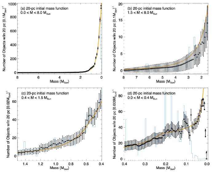
We now add these brown dwarf masses to the results of our Monte Carlo analysis of stellar masses above to produce a mass function across the entire mass range. This initial mass function is illustrated in Figure 20. Panel (a) shows the mass function across the full mass range from 0 to 8 , binned in 0.1 increments. The mass function rises with decreasing mass, and it continues to rise beyond our 0.025 () completeness limit. Subsequent panels show details. Panel (b) shows the high-mass end of the initial mass function from 1.5 to 8.0 , again with 0.1 binning. The statistics above 3 are poor but nonetheless show a steady increase from there down to 1.5. Panel (c) shows the mid-mass range (), now binned into smaller 0.02 increments because the statistics here are richer. Panel (d) zooms in on the smallest mass portion, below 0.4, and chooses yet a smaller mass binning of 0.005. With the exception of a few small features (discussed below), the mass function is seen to rise monotonically from 1.5 to 0.025. Mostly within the measurement errors (see more discussion below), the initial mass function is seen to continue rising well below our 0.025 completeness limit and at least down to 0.015.
The numbers on which Figure 20 is based are given in Table 22. For ease of reference, both the number of stars and the space density is given for each mass bin. Three mass binnings are tabulated, roughly paralleling what is shown in Figure 20: 0.1 binning across the entire 0.0-8.0 range (80 bins), 0.02 binning across the range 0.0-1.6 (80 bins), and 0.005 binning across the range 0.0-0.4 (80 bins). Mass bins with incomplete statistics are labeled as lower limits in the final column of the table.
| Mass Bin | Total # | Space DensityaaThe [ bin]-1 portion of the units should be replaced with the bin size for that row. For example, for the first row of the table, the units will be pc-3 []-1 because that bin is wide. | Lower Limit? |
|---|---|---|---|
| () | (pc-3 [ bin]-1) | ||
| (1) | (2) | (3) | (4) |
| 0.00-0.10 | 924.930.4 | 0.02760050.0009072 | yes |
| 0.10-0.20 | 761.028.9 | 0.02270940.0008624 | |
| 0.20-0.30 | 511.624.2 | 0.01526690.0007222 | |
| 0.30-0.40 | 351.720.5 | 0.01049530.0006118 | |
| 0.40-0.50 | 265.618.2 | 0.00792590.0005431 | |
| 0.50-0.60 | 214.316.8 | 0.00639500.0005013 | |
| 0.60-0.70 | 127.014.1 | 0.00378990.0004208 | |
| 0.70-0.80 | 94.512.6 | 0.00282000.0003760 |
Note. — (This table is available in its entirety in machine-readable form.)
There are a few features in Figure 20(c) and (d) that warrant special attention. The first is the bump in the object counts near 0.55 in panel (c). This falls near the point at which our mass estimation switches from that of the TIC relations of Stassun et al. (2019) at higher masses to that of the relation of Mann et al. (2019) at lower masses. Currently, we switch between these two relations at mag, corresponding to a mass of . As a test, if we change the switchover point to be at mag () instead, we find that this bump in the space densities moves to higher masses, with a deficit around , as shown in Figure 21. We also note that the uncertainties in the masses resulting from the Mann et al. (2019) relation are three to four times smaller than those derived from the Stassun et al. (2019) relation. As another test, we can artificially inflate the mass uncertainties on the Mann et al. (2019)-derived masses while keeping the current switchover point at mag. That result is also shown in Figure 21. In this case, the bump is greatly diminished in the number counts, but an inflection point is still seen near 0.6. Given that this feature in the number counts moves in response to the mass estimation used, we believe it is an artificial effect. Furthermore, given that the Stassun et al. (2019) mass estimation relies on dynamically measured individual masses whereas the Mann et al. (2019) relation uses Bayesian statistics to ferret out individual masses from binaries in which only the total system mass is measured, this likely indicates a small systematic offset that slightly deflates the Mann et al. (2019)-derived masses relative to truth. In fact, an effect in this direction and representing a systematic offset of is seen when comparing results of the relation to individually derived masses (figure 15 of Mann et al. 2019). Obtaining more directly measured individual masses in this regime, corresponding to late-K and early-M dwarfs, would help to put this issue to rest.
Other features are seen in Figure 20(d). There is a small drop in the number counts near 0.13 followed by a sudden rise near 0.11. This feature is likely artificial, as the bump at 0.11 is due primarily to components in multiple systems about which little information is known, and these were arbitrarily assigned masses of 0.11 based on an anticipated spectral type of M5.5. This type lies at a very sharp inflection point (see Table 20) in our mass vs. spectral type relation (Figure 14).
The other feature is the rapidly changing number count between masses of 0.06 and 0.08 , a mass range that straddles the stellar/substellar break. Some of the early- to mid-L dwarfs that we have included in our brown dwarf mass function analysis are likely very low-mass stars and not brown dwarfs themselves. As a consequence, these are assigned masses that are a bit too high (the extraneous high point in the 0.075-0.080 bin), which likely leads to concomitant deficits in the next higher mass bins. In fact, Table 3.1 lists three early-L dwarfs in the 20-pc census that have dynamical mass measurements, and one of these (LP 388-55 B; Dupuy & Liu 2017) has a mass just above the 0.075-0.080 mass bin (0.0830.03 ).
8 Discussion
How do our 20-pc results compare to other attempts in the literature to measure the initial mass function? Pioneering work by Salpeter (1955) found that a power law form with best fit the initial mass function over the range . Subsequent work by Miller & Scalo (1979) found for and for . Scalo (1986) determined for , and Reid et al. (2002) found for .
As more accurate measurements of the initial mass function became possible, researchers realized the importance of distinguishing whether the masses used for the computation were that of the stellar system or of its individual components. For example, in an analysis of data from the Sloan Digital Sky Survey, Bochanski et al. (2010) found for and for for the mass function of systems but and for the mass function of single stars over the same two mass regimes, respectively. Earlier, Kroupa (2001) had found that single-star initial mass functions resulting from the analysis of young star clusters generally gave values of that were higher by 0.5 (for ) than the field initial mass function, for which systems were not resolved. Reid (2005) cautions that unresolved multiplicity complicates interpretation of the initial mass function; the initial mass function of systems is more directly tied to the fragmentation of the original molecular cloud, but the initial mass function of individual objects give the mass distribution of the (sub)stellar bodies formed.
Our work on the 20-pc census has concentrated on analysis of the individual products of star formation, as we are curious to know how frequently this process produces, for example, very low-mass brown dwarfs compared to higher-mass objects. We will therefore restrict subsequent analysis here to the single-object initial mass function and leave analysis of the 20-pc census regarding multiplicity and the system mass function to those investigating how the formation of systems relates back to cloud fragmentation.
8.1 Comparison of Initial Mass Functions
Here we compare two very well established forms of the initial mass function and compare their predictions to our results based on the 20-pc census.
Chabrier (2001, 2003a, 2003b) developed several functional forms for the initial mass function. The latest one relating to single objects is given by Chabrier (2003b) and is comprised of a power law at high masses and a log-normal form at lower masses:
| (19) |
where , , , , and . The value of is in units of # of objects per pc3 per . See equation 2 and table 1 of Chabrier (2003b) for the derivation shown above. We note that the values of and are set by Chabrier (2003b) to match an empirical space density measurement (at 1 from Scalo 1986) of the initial mass function in the Milky Way’s disk population.
Likewise, Kroupa et al. (2013) found that a tripartite power-law form best describes the single-object initial mass function:
| (20) |
where , , and . As above, the value of is in units of # of objects per pc3 per . Note that there are two components of this mass function that contribute to the mass range . The value of is not specified by Kroupa et al. (2013). However, figure 4-24 of Kroupa et al. (2013) provides a comparison of this initial mass function with the Chabrier (2003b) version in Equation 19, showing that they are identical at 0.85, resulting in a value of .
As shown in Figure 22, neither of these parameterizations adequately describes the 20-pc initial mass function derived here. The main reason for this is that prior determinations were done pre-WISE, pre-Spitzer, and pre-Gaia before the L, T, and Y dwarf complement of the mass function was fully characterized and before exquisite parallax determinations became available for almost all objects in the 20-pc volume. As such, these prior works relied on poorer statistics with fits done in logarithmic scaling on both the and axes. Our careful accounting of objects within the 20-pc volume now allows for a more precise determination of the single-object initial mass function.
We thus provide a new multi-part power law parameterization that is bounded by the following caveats: (1) We assume at the high mass end, as has been determined from earlier studies, and we do this because our 20-pc census has few stars with to better constrain this. (2) We assume at intermediate masses, as this has also been established by earlier studies. (3) We take in the brown dwarf regime, as was determined in Section 7.1. We do not constrain the stitch points in mass between the power law pieces nor do we limit the number of power law pieces to only three. We perform these fits by eye, keeping in mind the caveats from Section 7.2 concerning the non-physical bumps and troughs in the number counts as a function of mass. Given the constraints above, we find that a three-piece power law does not adequately describe the number counts in the mid- to late-M dwarf regime (), but that a four-piece power law can. This best fit is given below and illustrated by the orange line in Figure 20:
| (21) |
where , , , , , , , , As above, the value of is in units of # of objects per pc3 per .
If we integrate under our best fit from 0.075 to 8.0 , we find 3002 stars, which can be compared to the 3000 individual objects in the 20-pc census that have (measured or implied) types of M9.5 or earlier. The integration under our fit for 0.020 to 0.075 gives 789 brown dwarfs, compared to the 582 individual L, T, and Y dwarfs in Table 3.1. Most of the missing brown dwarfs are ones with values 450-600K and distances of 15-20 pc or ones with 300-450K temperatures and 11-20 pc distances, where our current accounting is known to be incomplete (see Table 21). These results show that the number of stars relative to brown dwarfs is 3002/789, or 4. However, we believe that the brown dwarf mass function extends to at least 0.010 , which would give a ratio of 3002/986 (3) if the functional form continues to that mass. In the limiting case in which it continues to zero mass, we find a star-to-brown-dwarf ratio of 3002/1602, or . We note that as recently as a decade ago, this ratio in the Solar neighborhood was believed to be as high as 6:1 (Kirkpatrick et al. 2012).
This decrease in the ratio of stars to brown dwarfs is not in tension with microlensing results, as analysis of OGLE data found that an even steeper power law in the brown dwarf regime ( for ; Mróz et al. 2017) best fits the observed distribution of short-timescale (low-mass) events. Furthermore, the possibility that the mass function extends into a regime significantly below 0.010 is bolstered by recent JWST observations of the Orion Nebula Complex that show a significant population of objects, down to at least 0.001, that are apparently direct products of star formation (McCaughrean & Pearson 2023; Pearson & McCaughrean 2023).
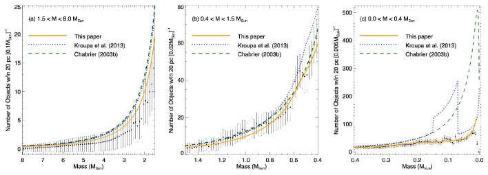
Finally, we note that our accounting of the mass of hydrogen-burning stars in the 20-pc census along with our best fit to the mass function of brown dwarfs allows us to calculate the average mass of an object in this sample. Integrating our mass function down to a mass of 0.020 , we find that value to be 0.41 . There are likely many undiscovered brown dwarfs in the solar neighborhood too faint to be currently detected, so this average value could be pushed lower. Assuming there is no low-mass cutoff of star formation and the brown dwarf mass function continues to zero mass with a power law slope of , we find that the average mass of objects in the 20-pc census would drop to 0.34 . This can be considered as the limiting case unless the functional form at the lowest masses has an value considerably greater than 0.6.
9 Conclusions
In this paper our aim was to study the initial mass distribution of star formation’s by-products, from the highest-mass progenitors of present-day white dwarfs to the lowest-mass brown dwarfs. For this, we have produced a volume-complete sample of stellar and substellar objects within 20 pc of the Sun. We have split multiple systems into their separate components and characterized each individual object to provide an accurate mass assignment.
Our main conclusions can be summarized as follows:
1) The initial mass function steadily increases as a function of descending mass. Its peak in (linear) mass space is not yet defined but is located below 0.020 (; Figure 20). We find that a quadripartite power-law () fits the observed space densities well (Equation 21). Going from high mass to low mass, we find exponents of 2.3, 1.3, 0.25, and 0.6, with stitch points between segments of 0.55, 0.22, and 0.05 , respectively. Although the rate of ascent of the mass function is slowly retarded as a function of descending mass through the stellar and high-mass brown dwarf regimes, its ascent increases again for the lower-mass brown dwarfs.
2) This initial mass function agrees well with previous determinations in the high-mass regime (by design) but differs markedly from other established formalisms in the M, L, T, and Y dwarf regimes (Section 8). Functional forms proposed by Chabrier (2003b) and Kroupa et al. (2013) overpredict the number of these lower-mass dwarfs relative to their more massive counterparts.
3) The 20-pc census currently consists of 3000 stars and 600 brown dwarfs (Table 3.1). At face value, this implies a stellar-to-substellar ratio of 5, but corrections for incompleteness for brown dwarfs with temperatures from 300-600K shows that the ratio is currently measured at 4. Incompletenesses at lower temperatures may yet bring this ratio as low as 3 (Section 8). The average mass of objects in the 20-pc census is currently measured as 0.41 but could drop as low as 0.34 if many colder brown dwarfs, yet to be discovered, actually exist (Section 8).
4) The 20-pc census of objects colder than 600K, corresponding to spectral type T8.5, is still incomplete beyond 15 pc, and the completeness volume shrinks to 11 pc at 450K, corresponding to spectral type Y0 (Table 21). Moreover, an additional source of incompleteness for objects as warm as 1350K is high backgrounds and confusion along the Galactic plane (Section 7.1).
5) There are direct indications that many unrecognized companions still exist to already identified members of the 20-pc census. Acceleration (aka proper motion anomaly) has been used to flag many such systems (Section 5.1.1), and large Gaia RUWE/LUWE values significantly higher than 1.0 flag many others (Section 5.2). Additional follow-up of these systems would help to better flesh out the 20-pc census itself while also providing much firmer statistics on multiplicity and the prevalence of hierarchical systems.
6) Our "complete" (see caveats #4 and #5, above) 20-pc census produced for this paper is available for additional uses (Table 3.1). As one example, this nearby sample is particularly useful as the hunting grounds for the closest habitable worlds to our own Solar System and is thus also available via the NASA Exoplanet Archive444444https://exoplanetarchive.ipac.caltech.edu/docs/20pcCensus.html.
7) Except for white dwarfs (Section 6.1.1) and brown dwarfs (Section 6.1.3), masses are used directly when they have been measured (Section 4). Most objects, though, lack actual mass determinations. For these we use a variety of mass estimation methods and select the ones that provide the most reliable results, when comparison to truth is available (Section 6.3). Nonetheless, our resulting space density computations binned by mass show some spurious features that appear to be caused by shortcomings in the estimation method. These are most obvious in the early-M dwarf region and in the regime from late-M to early-L dwarfs (Section 7.2). Dedicated programs, such as those by Vrijmoet et al. (2022) and Dupuy et al. (2022) directly determining masses of objects in these zones are clearly needed.
8) Dueling definitions in the literature of "brown dwarf" and "exoplanet" could bias our results if objects tagged as exoplanets are omitted from the initial mass function. We account for this and find that most of the objects labeled exoplanets (via the 13-based definition) fall in a small-mass regime separate from the objects that have been more traditionally labelled as brown dwarfs (via the formation-based definition) and do not affect our conclusions regarding the mass function (Section 6.2.3). This having been stated, future studies of the initial mass function might wisely consider no such division, as planet formation can be thought of merely as a (delayed) secondary process resulting from star formation itself. Including planetary formation products as another branch of the initial mass function will, however, not be feasible until a statistically robust, volume-complete set of exoplanets can be reliably measured.
9) Gaia DR3 detections comprise only of the volume-complete 20-pc census. Objects within 20 pc of the Sun can be missed by Gaia because they are too bright for Gaia observations, too faint for Gaia to detect, or are companions to Gaia-detected host stars that are (presently) inadequately characterized astrometrically (Section 2.1).
10) Citizen science continues to produce new discoveries within 20 pc (Section 2.1.2), even including a possible new Y dwarf with a "bonus" Spitzer parallax (Section A.3). Such discoveries are coming largely from WISE data sets, but these sets are being pushed to their sensitivity limits. Completing the 20-pc census in the 300-600K temperature range will require a deeper survey at 5 um, the best prospect for which is the NASA mission NEO Surveyor (Kirkpatrick et al. 2019b; Mainzer et al. 2023). Results from that mission, along with searches for cooler companions to known 20-pc hosts with JWST, represent our best short-term prospects for determining the occurrence rate of objects such as WISE J085510.83071442.5 that reside below 300K.
11) The 20-pc census enables us to identify the nearest star or brown dwarf in each constellation (Table 28). Interestingly, six of the eighty-eight constellations have a Y dwarf as their nearest member despite the fact that Y dwarfs have not yet been fully mapped within this 20-pc volume.
NOTE ADDED IN PROOF: The nearby brown dwarf candidate CWISE J165909.91351108.5 from Table 2 has been confirmed as a late-L dwarf by Robbins et al. (2023a), but it likely falls outside the 20-pc census. Additionally, Robbins et al. (2023b) find that CWISE J105512.11+544328.3, from Table 6.2.2, is not a T subdwarf but rather an anomalously blue Y dwarf.
ACKNOWLEDGMENTS: Davy Kirkpatrick, Federico Marocco, and Chris Gelino acknowledge support from grant #80NSSC20K0452 awarded for proposal 18-2ADAP18-0175 under the NASA Astrophysics Data Analysis Program. Data presented here are based on observations obtained at the Hale Telescope, Palomar Observatory as part of a continuing collaboration between the California Institute of Technology, NASA/JPL, Yale University, and the National Astronomical Observatories of China. Some of the data presented herein were obtained at the W. M. Keck Observatory, which is operated as a scientific partnership among the California Institute of Technology, the University of California and the National Aeronautics and Space Administration. The Observatory was made possible by the generous financial support of the W. M. Keck Foundation. The authors wish to recognize and acknowledge the very significant cultural role and reverence that the summit of Maunakea has always had within the indigenous Hawaiian community. We are most fortunate to have the opportunity to conduct observations from this mountain. This research has made use of the Keck Observatory Archive (KOA), which is operated by the W. M. Keck Observatory and the NASA Exoplanet Science Institute (NExScI), under contract with the National Aeronautics and Space Administration. The first author would like to thank Patrick Shopbell at Caltech for resurrecting an Exabyte drive that successfully read raw CTIO data from 1997. Part of this research was carried out at the Jet Propulsion Laboratory, California Institute of Technology, under a contract with the National Aeronautics and Space Administration (80NM0018D0004). He would also like to thank Mike Cushing for discussion of evolved star loci in the 20-pc color-magnitude diagrams.
One observation reported in this paper was obtained with the Southern African Large Telescope (SALT) under program 2021-2-SCI-027 (PI: Faherty). Roberto Raddi acknowledges support from Grant RYC2021-030837-I funded by MCIN/AEI/ 10.13039/501100011033 and by “European Union NextGenerationEU/PRTR”, and partial support by the AGAUR/Generalitat de Catalunya grant SGR-386/2021 and by the Spanish MINECO grant PID2020-117252GB-I00. Eileen Gonzales acknowledges support from the Heising-Simons Foundation through a 51 Pegasi b Fellowship. This publication makes use of VOSA, developed under the Spanish Virtual Observatory (https://svo.cab.inta-csic.es) project funded by MCIN/AEI/10.13039/501100011033/ through grant PID2020-112949GB-I00. This research made use of the Montreal Open Clusters and Associations (MOCA) database, operated at the Montréal Planétarium (J. Gagné et al., in preparation). Backyard Worlds research was supported by NASA grant 2017-ADAP17-0067 and by the NSF under grants AST- 2007068, AST-2009177, and AST-2009136. Johanna Vos acknowledges support from a Royal Society - Science Foundation Ireland University Research Fellowship (URF1221932).
References
- Abazajian et al. (2009) Abazajian, K. N., Adelman-McCarthy, J. K., Agüeros, M. A., et al. 2009, ApJS, 182, 543. doi:10.1088/0067-0049/182/2/543
- Aberasturi et al. (2014) Aberasturi, M., Burgasser, A. J., Mora, A., et al. 2014, AJ, 148, 129. doi:10.1088/0004-6256/148/6/129
- Aberasturi et al. (2014b) Aberasturi, M., Caballero, J. A., Montesinos, B., et al. 2014, AJ, 148, 36. doi:10.1088/0004-6256/148/2/36
- Abt (2017) Abt, H. A. 2017, PASP, 129, 044201. doi:10.1088/1538-3873/aa5b18
- Abt & Willmarth (2006) Abt, H. A. & Willmarth, D. 2006, ApJS, 162, 207. doi:10.1086/498095
- Abt (1981) Abt, H. A. 1981, ApJS, 45, 437. doi:10.1086/190719
- Abt & Levy (1976) Abt, H. A. & Levy, S. G. 1976, ApJS, 30, 273. doi:10.1086/190363
- Abt (1970) Abt, H. A. 1970, ApJS, 19, 387. doi:10.1086/190215
- Abt (1965) Abt, H. A. 1965, ApJS, 11, 429. doi:10.1086/190120
- Adams et al. (1935) Adams, W. S., Joy, A. H., Humason, M. L., et al. 1935, ApJ, 81, 187. doi:10.1086/143628
- Aerts (2021) Aerts, C. 2021, Reviews of Modern Physics, 93, 015001. doi:10.1103/RevModPhys.93.015001
- Affer et al. (2016) Affer, L., Micela, G., Damasso, M., et al. 2016, A&A, 593, A117. doi:10.1051/0004-6361/201628690
- Affer et al. (2005) Affer, L., Micela, G., Morel, T., et al. 2005, A&A, 433, 647. doi:10.1051/0004-6361:20041308
- Agati et al. (2015) Agati, J.-L., Bonneau, D., Jorissen, A., et al. 2015, A&A, 574, A6. doi:10.1051/0004-6361/201323056
- Akeson et al. (2021) Akeson, R., Beichman, C., Kervella, P., et al. 2021, AJ, 162, 14. doi:10.3847/1538-3881/abfaff
- Albert et al. (2011) Albert, L., Artigau, É., Delorme, P., et al. 2011, AJ, 141, 203. doi:10.1088/0004-6256/141/6/203
- Alberts et al. (1996) Alberts, F., Savonije, G. J., van den Heuvel, E. P. J., et al. 1996, Nature, 380, 676. doi:10.1038/380676a0
- Allen et al. (2000) Allen, C., Poveda, A., & Herrera, M. A. 2000, A&A, 356, 529
- Allen et al. (2012) Allen, P. R., Burgasser, A. J., Faherty, J. K., et al. 2012, AJ, 144, 62. doi:10.1088/0004-6256/144/2/62
- Allen (1899) Allen, R. H. 1899, New York, Leipzig [etc.] G.E. Stechert, 1899.
- Allende Prieto & Lambert (1999) Allende Prieto, C. & Lambert, D. L. 1999, A&A, 352, 555
- Allers & Liu (2013) Allers, K. N. & Liu, M. C. 2013, ApJ, 772, 79. doi:10.1088/0004-637X/772/2/79
- Alonso-Floriano et al. (2015) Alonso-Floriano, F. J., Morales, J. C., Caballero, J. A., et al. 2015, A&A, 577, A128. doi:10.1051/0004-6361/201525803
- Amado et al. (2021) Amado, P. J., Bauer, F. F., Rodríguez López, C., et al. 2021, A&A, 650, A188. doi:10.1051/0004-6361/202140633
- Ammler-von Eiff et al. (2016) Ammler-von Eiff, M., Bedalov, A., Kranhold, C., et al. 2016, A&A, 591, A84. doi:10.1051/0004-6361/201526625
- Anders et al. (2022) Anders, F., Khalatyan, A., Queiroz, A. B. A., et al. 2022, A&A, 658, A91. doi:10.1051/0004-6361/202142369
- Andersen et al. (2008) Andersen, M., Meyer, M. R., Greissl, J., et al. 2008, ApJ, 683, L183. doi:10.1086/591473
- Andrade (2019) Andrade, M. 2019, A&A, 630, A96. doi:10.1051/0004-6361/201936199
- Andrews et al. (2019) Andrews, J. J., Breivik, K., & Chatterjee, S. 2019, ApJ, 886, 68. doi:10.3847/1538-4357/ab441f
- Andrews et al. (2015) Andrews, J. J., Agüeros, M. A., Gianninas, A., et al. 2015, ApJ, 815, 63. doi:10.1088/0004-637X/815/1/63
- Anglada-Escude et al. (2014) Anglada-Escude, G., Arriagada, P., Tuomi, M., et al. 2014, MNRAS, 443, L89. doi:10.1093/mnrasl/slu076
- Apps et al. (2010) Apps, K., Clubb, K. I., Fischer, D. A., et al. 2010, PASP, 122, 156. doi:10.1086/651058
- Arenou et al. (2000) Arenou, F., Halbwachs, J.-L., Mayor, M., et al. 2000, IAU Symposium, 200, 135
- Argelander (1903) Argelander, F. W. A. 1903, Eds Marcus and Weber’s Verlag, 0
- Artigau et al. (2010) Artigau, É., Radigan, J., Folkes, S., et al. 2010, ApJ, 718, L38. doi:10.1088/2041-8205/718/1/L38
- Astudillo-Defru et al. (2017) Astudillo-Defru, N., Forveille, T., Bonfils, X., et al. 2017, A&A, 602, A88. doi:10.1051/0004-6361/201630153
- Azulay et al. (2017) Azulay, R., Guirado, J. C., Marcaide, J. M., et al. 2017, A&A, 607, A10. doi:10.1051/0004-6361/201730641
- Azulay et al. (2015) Azulay, R., Guirado, J. C., Marcaide, J. M., et al. 2015, A&A, 578, A16. doi:10.1051/0004-6361/201525704
- Bach et al. (2009) Bach, K., Lee, J., Demarque, P., et al. 2009, ApJ, 703, 362. doi:10.1088/0004-637X/703/1/362
- Bagnulo & Landstreet (2020) Bagnulo, S. & Landstreet, J. D. 2020, A&A, 643, A134. doi:10.1051/0004-6361/202038565
- Bailer-Jones (2022) Bailer-Jones, C. A. L. 2022, ApJ, 935, L9. doi:10.3847/2041-8213/ac816a
- Baines et al. (2018) Baines, E. K., Armstrong, J. T., Schmitt, H. R., et al. 2018, AJ, 155, 30. doi:10.3847/1538-3881/aa9d8b
- Baines & Armstrong (2012) Baines, E. K. & Armstrong, J. T. 2012, ApJ, 744, 138. doi:10.1088/0004-637X/744/2/138
- Bakos et al. (2006) Bakos, G. Á., Pál, A., Latham, D. W., et al. 2006, ApJ, 641, L57. doi:10.1086/503671
- Balega et al. (2013) Balega, I. I., Balega, Y. Y., Gasanova, L. T., et al. 2013, Astrophysical Bulletin, 68, 53. doi:10.1134/S1990341313010057
- Balega et al. (2004) Balega, I., Balega, Y. Y., Maksimov, A. F., et al. 2004, A&A, 422, 627. doi:10.1051/0004-6361:20035705
- Balega et al. (1984) Balega, I., Bonneau, D., & Foy, R. 1984, A&AS, 57, 31
- Baraffe et al. (2003) Baraffe, I., Chabrier, G., Barman, T. S., et al. 2003, A&A, 402, 701. doi:10.1051/0004-6361:20030252
- Bardalez Gagliuffi et al. (2020) Bardalez Gagliuffi, D. C., Faherty, J. K., Schneider, A. C., et al. 2020, ApJ, 895, 145. doi:10.3847/1538-4357/ab8d25
- Bardalez Gagliuffi et al. (2019) Bardalez Gagliuffi, D. C., Burgasser, A. J., Schmidt, S. J., et al. 2019, ApJ, 883, 205. doi:10.3847/1538-4357/ab253d
- Bardalez Gagliuffi et al. (2014) Bardalez Gagliuffi, D. C., Burgasser, A. J., Gelino, C. R., et al. 2014, ApJ, 794, 143. doi:10.1088/0004-637X/794/2/143
- Baroch et al. (2021) Baroch, D., Morales, J. C., Ribas, I., et al. 2021, A&A, 653, A49. doi:10.1051/0004-6361/202141031
- Baroch et al. (2018) Baroch, D., Morales, J. C., Ribas, I., et al. 2018, A&A, 619, A32. doi:10.1051/0004-6361/201833440
- Barrientos & Chanamé (2021) Barrientos, M. & Chanamé, J. 2021, ApJ, 923, 181. doi:10.3847/1538-4357/ac2f49
- Barry et al. (2012) Barry, R. K., Demory, B.-O., Ségransan, D., et al. 2012, ApJ, 760, 55. doi:10.1088/0004-637X/760/1/55
- Bartlett et al. (2017) Bartlett, J. L., Lurie, J. C., Riedel, A., et al. 2017, AJ, 154, 151. doi:10.3847/1538-3881/aa8457
- Bastian et al. (2010) Bastian, N., Covey, K. R., & Meyer, M. R. 2010, ARA&A, 48, 339. doi:10.1146/annurev-astro-082708-101642
- Batten & Fletcher (1992) Batten, A. H. & Fletcher, J. M. 1992, JRASC, 86, 99
- Batten et al. (1978) Batten, A. H., Fletcher, J. M., & Mann, P. J. 1978, Publications of the Dominion Astrophysical Observatory Victoria, 15, 121
- Bauer et al. (2020) Bauer, F. F., Zechmeister, M., Kaminski, A., et al. 2020, A&A, 640, A50. doi:10.1051/0004-6361/202038031
- Bayer (1603) Bayer, J. 1603, Uranometria omnium asterismorum continens schemata, nova methodo delineata aereis laminis expressa, by Bayer, Johann; Augsburg: excudit Christophorus Mangus (1603). doi:10.3931/e-rara-309
- Bayo et al. (2008) Bayo, A., Rodrigo, C., Barrado Y Navascués, D., et al. 2008, A&A, 492, 277. doi:10.1051/0004-6361:200810395
- Bazot et al. (2018) Bazot, M., Creevey, O., Christensen-Dalsgaard, J., et al. 2018, A&A, 619, A172. doi:10.1051/0004-6361/201834058
- Bazot et al. (2011) Bazot, M., Ireland, M. J., Huber, D., et al. 2011, A&A, 526, L4. doi:10.1051/0004-6361/201015679
- Beamín et al. (2013) Beamín, J. C., Minniti, D., Gromadzki, M., et al. 2013, A&A, 557, L8. doi:10.1051/0004-6361/201322190
- Beard et al. (2022) Beard, C., Robertson, P., Kanodia, S., et al. 2022, ApJ, 936, 55. doi:10.3847/1538-4357/ac8480
- Beavers & Salzer (1985) Beavers, W. I. & Salzer, J. J. 1985, PASP, 97, 355. doi:10.1086/131545
- Bédard et al. (2017) Bédard, A., Bergeron, P., & Fontaine, G. 2017, ApJ, 848, 11. doi:10.3847/1538-4357/aa8bb6
- Beichman et al. (2011) Beichman, C. A., Lisse, C. M., Tanner, A. M., et al. 2011, ApJ, 743, 85. doi:10.1088/0004-637X/743/1/85
- Belokurov et al. (2020) Belokurov, V., Penoyre, Z., Oh, S., et al. 2020, MNRAS, 496, 1922. doi:10.1093/mnras/staa1522
- Benedict et al. (2016) Benedict, G. F., Henry, T. J., Franz, O. G., et al. 2016, AJ, 152, 141. doi:10.3847/0004-6256/152/5/141
- Benedict et al. (2001) Benedict, G. F., McArthur, B. E., Franz, O. G., et al. 2001, AJ, 121, 1607. doi:10.1086/319399
- Benjamin et al. (2003) Benjamin, R. A., Churchwell, E., Babler, B. L., et al. 2003, PASP, 115, 953. doi:10.1086/376696
- Bensby et al. (2014) Bensby, T., Feltzing, S., & Oey, M. S. 2014, A&A, 562, A71. doi:10.1051/0004-6361/201322631
- Berdnikov & Pastukhova (2008) Berdnikov, L. N. & Pastukhova, E. N. 2008, Peremennye Zvezdy, 28, 9
- Bergeron et al. (2022) Bergeron, P., Kilic, M., Blouin, S., et al. 2022, ApJ, 934, 36. doi:10.3847/1538-4357/ac76c7
- Bergeron et al. (2019) Bergeron, P., Dufour, P., Fontaine, G., et al. 2019, ApJ, 876, 67. doi:10.3847/1538-4357/ab153a
- Bergeron et al. (2001) Bergeron, P., Leggett, S. K., & Ruiz, M. T. 2001, ApJS, 133, 413. doi:10.1086/320356
- Bergeron et al. (1997) Bergeron, P., Ruiz, M. T., & Leggett, S. K. 1997, ApJS, 108, 339. doi:10.1086/312955
- Bergeron et al. (1994) Bergeron, P., Ruiz, M.-T., Leggett, S. K., et al. 1994, ApJ, 423, 456. doi:10.1086/173823
- Bergeron et al. (1992) Bergeron, P., Saffer, R. A., & Liebert, J. 1992, ApJ, 394, 228. doi:10.1086/171575
- Bergfors et al. (2016) Bergfors, C., Brandner, W., Bonnefoy, M., et al. 2016, MNRAS, 456, 2576. doi:10.1093/mnras/stv2768
- Bergfors et al. (2010) Bergfors, C., Brandner, W., Janson, M., et al. 2010, A&A, 520, A54. doi:10.1051/0004-6361/201014114
- Bernat et al. (2010) Bernat, D., Bouchez, A. H., Ireland, M., et al. 2010, ApJ, 715, 724. doi:10.1088/0004-637X/715/2/724
- Bernkopf et al. (2012) Bernkopf, J., Chini, R., Buda, L.-S., et al. 2012, MNRAS, 425, 1308. doi:10.1111/j.1365-2966.2012.21534.x
- Berski & Dybczyński (2016) Berski, F. & Dybczyński, P. A. 2016, A&A, 595, L10. doi:10.1051/0004-6361/201629835
- Bessel (1844) Bessel, F. W. 1844, MNRAS, 6, 136. doi:10.1093/mnras/6.11.136
- Best et al. (2021) Best, W. M. J., Liu, M. C., Magnier, E. A., et al. 2021, AJ, 161, 42. doi:10.3847/1538-3881/abc893
- Best et al. (2020) Best, W. M. J., Liu, M. C., Magnier, E. A., et al. 2020, AJ, 159, 257. doi:10.3847/1538-3881/ab84f4
- Best et al. (2015) Best, W. M. J., Liu, M. C., Magnier, E. A., et al. 2015, ApJ, 814, 118. doi:10.1088/0004-637X/814/2/118
- Best et al. (2013) Best, W. M. J., Liu, M. C., Magnier, E. A., et al. 2013, ApJ, 777, 84. doi:10.1088/0004-637X/777/2/84
- Beuzit et al. (2004) Beuzit, J.-L., Ségransan, D., Forveille, T., et al. 2004, A&A, 425, 997. doi:10.1051/0004-6361:20048006
- Bidelman (1980) Bidelman, W. P. 1980, PASP, 92, 345. doi:10.1086/130674
- Bidelman (1985) Bidelman, W. P. 1985, ApJS, 59, 197. doi:10.1086/191069
- Bihain et al. (2013) Bihain, G., Scholz, R.-D., Storm, J., et al. 2013, A&A, 557, A43. doi:10.1051/0004-6361/201322141
- Biller et al. (2022) Biller, B. A., Grandjean, A., Messina, S., et al. 2022, A&A, 658, A145. doi:10.1051/0004-6361/202142438
- Blomme et al. (2022) Blomme, R., Fremat, Y., Sartoretti, P., et al. 2022, arXiv:2206.05486
- Blouin et al. (2019) Blouin, S., Dufour, P., Thibeault, C., et al. 2019, ApJ, 878, 63. doi:10.3847/1538-4357/ab1f82
- Bobylev & Bajkova (2022) Bobylev, V. & Bajkova, A. 2022, arXiv:2206.14443. doi:10.48550/arXiv.2206.14443
- Boccaletti et al. (2003) Boccaletti, A., Chauvin, G., Lagrange, A.-M., et al. 2003, A&A, 410, 283. doi:10.1051/0004-6361:20031216
- Bochanski et al. (2010) Bochanski, J. J., Hawley, S. L., Covey, K. R., et al. 2010, AJ, 139, 2679. doi:10.1088/0004-6256/139/6/2679
- Bochanski et al. (2009) Bochanski, J. J., Hennawi, J. F., Simcoe, R. A., et al. 2009, PASP, 121, 1409. doi:10.1086/648597
- Bochanski et al. (2005) Bochanski, J. J., Hawley, S. L., Reid, I. N., et al. 2005, AJ, 130, 1871. doi:10.1086/444417
- Boden et al. (1999) Boden, A. F., Koresko, C. D., van Belle, G. T., et al. 1999, ApJ, 515, 356. doi:10.1086/307030
- Boeshaar & Tyson (1985) Boeshaar, P. C. & Tyson, J. A. 1985, AJ, 90, 817. doi:10.1086/113791
- Boeshaar (1976) Boeshaar, P. C. 1976, Ph.D. Thesis
- Bonavita & Desidera (2020) Bonavita, M. & Desidera, S. 2020, Galaxies, 8, 16. doi:10.3390/galaxies8010016
- Bond et al. (2020) Bond, H. E., Schaefer, G. H., Gilliland, R. L., et al. 2020, ApJ, 904, 112. doi:10.3847/1538-4357/abc172
- Bond et al. (2018) Bond, H. E., Gilliland, R. L., Schaefer, G. H., et al. 2018, Research Notes of the American Astronomical Society, 2, 147. doi:10.3847/2515-5172/aad9a4
- Bond et al. (2017) Bond, H. E., Schaefer, G. H., Gilliland, R. L., et al. 2017, ApJ, 840, 70. doi:10.3847/1538-4357/aa6af8
- Bonfils et al. (2018) Bonfils, X., Almenara, J.-M., Cloutier, R., et al. 2018, A&A, 618, A142. doi:10.1051/0004-6361/201731884
- Bonfils et al. (2018b) Bonfils, X., Astudillo-Defru, N., Díaz, R., et al. 2018b, A&A, 613, A25. doi:10.1051/0004-6361/201731973
- Bonfils et al. (2013) Bonfils, X., Delfosse, X., Udry, S., et al. 2013, A&A, 549, A109. doi:10.1051/0004-6361/201014704
- Bonfils et al. (2007) Bonfils, X., Mayor, M., Delfosse, X., et al. 2007, A&A, 474, 293. doi:10.1051/0004-6361:20077068
- Bonfils et al. (2005) Bonfils, X., Delfosse, X., Udry, S., et al. 2005, A&A, 442, 635. doi:10.1051/0004-6361:20053046
- Bonnefoy et al. (2018) Bonnefoy, M., Perraut, K., Lagrange, A.-M., et al. 2018, A&A, 618, A63. doi:10.1051/0004-6361/201832942
- Bonnefoy et al. (2014) Bonnefoy, M., Chauvin, G., Lagrange, A.-M., et al. 2014, A&A, 562, A127. doi:10.1051/0004-6361/201118270
- Borgniet et al. (2019) Borgniet, S., Lagrange, A.-M., Meunier, N., et al. 2019, A&A, 621, A87. doi:10.1051/0004-6361/201833431
- Borsa et al. (2015) Borsa, F., Scandariato, G., Rainer, M., et al. 2015, A&A, 578, A64. doi:10.1051/0004-6361/201525741
- Bouy et al. (2005) Bouy, H., Martín, E. L., Brandner, W., et al. 2005, AJ, 129, 511. doi:10.1086/426559
- Bouy et al. (2004) Bouy, H., Duchêne, G., Köhler, R., et al. 2004, A&A, 423, 341. doi:10.1051/0004-6361:20040551
- Bouy et al. (2003) Bouy, H., Brandner, W., Martín, E. L., et al. 2003, AJ, 126, 1526. doi:10.1086/377343
- Bowler et al. (2023) Bowler, B. P., Tran, Q. H., Zhang, Z., et al. 2023, AJ, 165, 164. doi:10.3847/1538-3881/acbd34
- Bowler et al. (2020) Bowler, B. P., Blunt, S. C., & Nielsen, E. L. 2020, AJ, 159, 63. doi:10.3847/1538-3881/ab5b11
- Bowler et al. (2019) Bowler, B. P., Hinkley, S., Ziegler, C., et al. 2019, ApJ, 877, 60. doi:10.3847/1538-4357/ab1018
- Bowler et al. (2015a) Bowler, B. P., Liu, M. C., Shkolnik, E. L., et al. 2015a, ApJS, 216, 7. doi:10.1088/0067-0049/216/1/7
- Bowler et al. (2015b) Bowler, B. P., Shkolnik, E. L., Liu, M. C., et al. 2015b, ApJ, 806, 62. doi:10.1088/0004-637X/806/1/62
- Boyajian et al. (2012) Boyajian, T. S., McAlister, H. A., van Belle, G., et al. 2012, ApJ, 746, 101. doi:10.1088/0004-637X/746/1/101
- Boyd et al. (2011) Boyd, M. R., Henry, T. J., Jao, W.-C., et al. 2011, AJ, 142, 92. doi:10.1088/0004-6256/142/3/92
- Brandão et al. (2011) Brandão, I. M., Doğan, G., Christensen-Dalsgaard, J., et al. 2011, A&A, 527, A37. doi:10.1051/0004-6361/201015370
- Brandt et al. (2021) Brandt, G. M., Dupuy, T. J., Li, Y., et al. 2021, AJ, 162, 301. doi:10.3847/1538-3881/ac273e
- Brandt (2021) Brandt, T. D. 2021, ApJS, 254, 42. doi:10.3847/1538-4365/abf93c
- Brandt et al. (2020) Brandt, T. D., Dupuy, T. J., Bowler, B. P., et al. 2020, AJ, 160, 196. doi:10.3847/1538-3881/abb45e
- Brandt et al. (2019) Brandt, T. D., Dupuy, T. J., & Bowler, B. P. 2019, AJ, 158, 140. doi:10.3847/1538-3881/ab04a8
- Brandt et al. (2014) Brandt, T. D., McElwain, M. W., Turner, E. L., et al. 2014, ApJ, 794, 159. doi:10.1088/0004-637X/794/2/159
- Breakiron & Gatewood (1974) Breakiron, L. A. & Gatewood, G. 1974, PASP, 86, 448. doi:10.1086/129629
- Bressan et al. (2012) Bressan, A., Marigo, P., Girardi, L., et al. 2012, MNRAS, 427, 127. doi:10.1111/j.1365-2966.2012.21948.x
- Brewer et al. (2016) Brewer, J. M., Fischer, D. A., Valenti, J. A., et al. 2016, ApJS, 225, 32. doi:10.3847/0067-0049/225/2/32
- Brown et al. (1991) Brown, T. M., Gilliland, R. L., Noyes, R. W., et al. 1991, ApJ, 368, 599. doi:10.1086/169725
- Bruntt et al. (2010) Bruntt, H., Bedding, T. R., Quirion, P.-O., et al. 2010, MNRAS, 405, 1907. doi:10.1111/j.1365-2966.2010.16575.x
- Buckley et al. (2006) Buckley, D. A. H., Swart, G. P., & Meiring, J. G. 2006, Proc. SPIE, 6267, 62670Z. doi:10.1117/12.673750
- Burgasser et al. (2015a) Burgasser, A. J., Gillon, M., Melis, C., et al. 2015a, AJ, 149, 104. doi:10.1088/0004-6256/149/3/104
- Burgasser et al. (2015b) Burgasser, A. J., Melis, C., Todd, J., et al. 2015b, AJ, 150, 180. doi:10.1088/0004-6256/150/6/180
- Burgasser et al. (2013) Burgasser, A. J., Sheppard, S. S., & Luhman, K. L. 2013, ApJ, 772, 129. doi:10.1088/0004-637X/772/2/129
- Burgasser et al. (2011) Burgasser, A. J., Sitarski, B. N., Gelino, C. R., et al. 2011, ApJ, 739, 49. doi:10.1088/0004-637X/739/1/49
- Burgasser et al. (2010a) Burgasser, A. J., Looper, D., & Rayner, J. T. 2010a, AJ, 139, 2448. doi:10.1088/0004-6256/139/6/2448
- Burgasser et al. (2010b) Burgasser, A. J., Cruz, K. L., Cushing, M., et al. 2010b, ApJ, 710, 1142. doi:10.1088/0004-637X/710/2/1142
- Burgasser et al. (2008) Burgasser, A. J., Looper, D. L., Kirkpatrick, J. D., et al. 2008a, ApJ, 674, 451. doi:10.1086/524726
- Burgasser et al. (2008b) Burgasser, A. J., Liu, M. C., Ireland, M. J., et al. 2008b, ApJ, 681, 579. doi:10.1086/588379
- Burgasser et al. (2007) Burgasser, A. J., Looper, D. L., Kirkpatrick, J. D., et al. 2007, ApJ, 658, 557. doi:10.1086/511518
- Burgasser (2007b) Burgasser, A. J. 2007, ApJ, 659, 655. doi:10.1086/511027
- Burgasser et al. (2007c) Burgasser, A. J., Cruz, K. L., & Kirkpatrick, J. D. 2007c, ApJ, 657, 494. doi:10.1086/510148
- Burgasser et al. (2006) Burgasser, A. J., Geballe, T. R., Leggett, S. K., et al. 2006, ApJ, 637, 1067. doi:10.1086/498563
- Burgasser et al. (2004) Burgasser, A. J., McElwain, M. W., Kirkpatrick, J. D., et al. 2004, AJ, 127, 2856. doi:10.1086/383549
- Burgasser et al. (2003) Burgasser, A. J., Kirkpatrick, J. D., Liebert, J., et al. 2003, ApJ, 594, 510. doi:10.1086/376756
- Burgh et al. (2003) Burgh, E. B., Nordsieck, K. H., Kobulnicky, H. A., et al. 2003, Proc. SPIE, 4841, 1463. doi:10.1117/12.460312
- Burningham et al. (2014) Burningham, B., Smith, L., Cardoso, C. V., et al. 2014, MNRAS, 440, 359. doi:10.1093/mnras/stu184
- Burningham et al. (2013) Burningham, B., Cardoso, C. V., Smith, L., et al. 2013, MNRAS, 433, 457. doi:10.1093/mnras/stt740
- Burningham et al. (2011) Burningham, B., Lucas, P. W., Leggett, S. K., et al. 2011, MNRAS, 414, L90. doi:10.1111/j.1745-3933.2011.01062.x
- Burningham et al. (2010) Burningham, B., Pinfield, D. J., Lucas, P. W., et al. 2010, MNRAS, 406, 1885. doi:10.1111/j.1365-2966.2010.16800.x
- Burrows et al. (1997) Burrows, A., Marley, M., Hubbard, W. B., et al. 1997, ApJ, 491, 856. doi:10.1086/305002
- Burt et al. (2021) Burt, J., Feng, F., Holden, B., et al. 2021, AJ, 161, 10. doi:10.3847/1538-3881/abc2d0
- Butler et al. (2017) Butler, R. P., Vogt, S. S., Laughlin, G., et al. 2017, AJ, 153, 208. doi:10.3847/1538-3881/aa66ca
- Butler et al. (2006) Butler, R. P., Wright, J. T., Marcy, G. W., et al. 2006, ApJ, 646, 505. doi:10.1086/504701
- Bychkov et al. (2013) Bychkov, V. D., Bychkova, L. V., & Madej, J. 2013, AJ, 146, 74. doi:10.1088/0004-6256/146/4/74
- Calamari et al. (2022) Calamari, E., Faherty, J. K., Burningham, B., et al. 2022, ApJ, 940, 164. doi:10.3847/1538-4357/ac9cc9
- Calissendorff et al. (2023) Calissendorff, P., De Furio, M., Meyer, M., et al. 2023, ApJ, 947, L30. doi:10.3847/2041-8213/acc86d
- Calissendorff et al. (2020) Calissendorff, P., Janson, M., & Bonnefoy, M. 2020, A&A, 642, A57. doi:10.1051/0004-6361/202038030
- Cannon & Pickering (1993) Cannon, A. J. & Pickering, E. C. 1993, VizieR Online Data Catalog, III/135A
- Cannon & Mayall (1949) Cannon, A. J. & Mayall, M. W. 1949, Annals of Harvard College Observatory, 112, 1
- Cannon (1936) Cannon, A. J. 1936, Annals of Harvard College Observatory, 100, 205
- Cannon (1931) Cannon, A. J. 1931, Annals of Harvard College Observatory, 100, 61
- Cannon (1928) Cannon, A. J. 1928, Annals of Harvard College Observatory, 100, 49
- Cannon (1927) Cannon, A. J. 1927, Annals of Harvard College Observatory, 100, 33
- Cannon (1925a) Cannon, A. J. 1925a, Annals of Harvard College Observatory, 100, 1
- Cannon (1925b) Cannon, A. J. 1925b, Annals of Harvard College Observatory, 100, 17
- Cannon & Pickering (1924) Cannon, A. J. & Pickering, E. C. 1924, Annals of Harvard College Observatory, 99, 1
- Cannon & Pickering (1923) Cannon, A. J. & Pickering, E. C. 1923, Annals of Harvard College Observatory, 98, 1
- Cannon & Pickering (1922) Cannon, A. J. & Pickering, E. C. 1922, Annals of Harvard College Observatory, 97, 1
- Cannon & Pickering (1921) Cannon, A. J. & Pickering, E. C. 1921, Annals of Harvard College Observatory, 96, 1
- Cannon & Pickering (1920) Cannon, A. J. & Pickering, E. C. 1920, Annals of Harvard College Observatory, 95, 1
- Cannon & Pickering (1919a) Cannon, A. J. & Pickering, E. C. 1919a, Annals of Harvard College Observatory, 93, 1
- Cannon & Pickering (1919b) Cannon, A. J. & Pickering, E. C. 1919b, Annals of Harvard College Observatory, 94, 1
- Cannon & Pickering (1918a) Cannon, A. J. & Pickering, E. C. 1918a, Annals of Harvard College Observatory, 91, 1
- Cannon & Pickering (1918b) Cannon, A. J. & Pickering, E. C. 1918b, Annals of Harvard College Observatory, 92, 1
- Cardona Guillén et al. (2021) Cardona Guillén, C., Lodieu, N., Béjar, V. J. S., et al. 2021, A&A, 654, A134. doi:10.1051/0004-6361/202141122
- Carey et al. (2009) Carey, S. J., Noriega-Crespo, A., Mizuno, D. R., et al. 2009, PASP, 121, 76. doi:10.1086/596581
- Carrier et al. (2005) Carrier, F., Eggenberger, P., & Bouchy, F. 2005, A&A, 434, 1085. doi:10.1051/0004-6361:20042140
- Carroll & Ostlie (1996) Carroll, B. W. & Ostlie, D. A. 1996, An Introduction to Modern Astrophysics, by B.W. Carroll and D.A. Ostlie. Benjamin Cummings, 1996. ISBN 0-201-54730-9.
- Caselden et al. (2018) Caselden, D., Westin, P., Meisner, A., et al. 2018, Astrophysics Source Code Library. ascl:1806.004
- Castro et al. (2013) Castro, P. J., Gizis, J. E., Harris, H. C., et al. 2013, ApJ, 776, 126. doi:10.1088/0004-637X/776/2/126
- Catalán et al. (2008) Catalán, S., Isern, J., García-Berro, E., et al. 2008, A&A, 477, 213. doi:10.1051/0004-6361:20078111
- Catalán et al. (2008b) Catalán, S., Ribas, I., Isern, J., et al. 2008b, A&A, 477, 901. doi:10.1051/0004-6361:20078230
- Chabrier (2003b) Chabrier, G. 2003, PASP, 115, 763. doi:10.1086/376392
- Chabrier (2003a) Chabrier, G. 2003, ApJ, 586, L133. doi:10.1086/374879
- Chabrier (2001) Chabrier, G. 2001, ApJ, 554, 1274. doi:10.1086/321401
- Chandra et al. (2020) Chandra, V., Hwang, H.-C., Zakamska, N. L., et al. 2020, ApJ, 899, 146. doi:10.3847/1538-4357/aba8a2
- Chauvin et al. (2007) Chauvin, G., Lagrange, A.-M., Udry, S., et al. 2007, A&A, 475, 723. doi:10.1051/0004-6361:20067046
- Chauvin et al. (2004) Chauvin, G., Lagrange, A.-M., Dumas, C., et al. 2004, A&A, 425, L29. doi:10.1051/0004-6361:200400056
- Che et al. (2011) Che, X., Monnier, J. D., Zhao, M., et al. 2011, ApJ, 732, 68. doi:10.1088/0004-637X/732/2/68
- Chen et al. (2022) Chen, M., Li, Y., Brandt, T. D., et al. 2022, AJ, 163, 288. doi:10.3847/1538-3881/ac66d2
- Chini et al. (2014) Chini, R., Fuhrmann, K., Barr, A., et al. 2014, MNRAS, 437, 879. doi:10.1093/mnras/stt1953
- Chiu et al. (2006) Chiu, K., Fan, X., Leggett, S. K., et al. 2006, AJ, 131, 2722. doi:10.1086/501431
- Chontos et al. (2021) Chontos, A., Huber, D., Berger, T. A., et al. 2021, ApJ, 922, 229. doi:10.3847/1538-4357/ac1269
- Christian et al. (2003) Christian, D. J., Mathioudakis, M., Jevremović, D., et al. 2003, ApJ, 593, L105. doi:10.1086/378217
- Christian et al. (2001) Christian, D. J., Craig, N., Dupuis, J., et al. 2001, AJ, 122, 378. doi:10.1086/321124
- Cifuentes et al. (2020) Cifuentes, C., Caballero, J. A., Cortés-Contreras, M., et al. 2020, A&A, 642, A115. doi:10.1051/0004-6361/202038295
- Clark et al. (2022) Clark, C. A., van Belle, G. T., Horch, E. P., et al. 2022, AJ, 164, 33. doi:10.3847/1538-3881/ac739c
- Climent et al. (2019) Climent, J. B., Berger, J. P., Guirado, J. C., et al. 2019, ApJ, 886, L9. doi:10.3847/2041-8213/ab5065
- Close et al. (2007) Close, L. M., Thatte, N., Nielsen, E. L., et al. 2007, ApJ, 665, 736. doi:10.1086/518207
- Cloutier et al. (2021) Cloutier, R., Charbonneau, D., Deming, D., et al. 2021, AJ, 162, 174. doi:10.3847/1538-3881/ac1584
- Compton et al. (2019) Compton, D. L., Bedding, T. R., & Stello, D. 2019, MNRAS, 485, 560. doi:10.1093/mnras/stz432
- Corbally (1984) Corbally, C. J. 1984, ApJS, 55, 657. doi:10.1086/190973
- Cortés-Contreras et al. (2017) Cortés-Contreras, M., Béjar, V. J. S., Caballero, J. A., et al. 2017, A&A, 597, A47. doi:10.1051/0004-6361/201629056
- Cowley (1976) Cowley, A. P. 1976, PASP, 88, 95. doi:10.1086/129905
- Cowley et al. (1967) Cowley, A. P., Hiltner, W. A., & Witt, A. N. 1967, AJ, 72, 1334. doi:10.1086/110413
- Creevey et al. (2012) Creevey, O. L., Thévenin, F., Boyajian, T. S., et al. 2012, A&A, 545, A17. doi:10.1051/0004-6361/201219651
- Crifo et al. (2005) Crifo, F., Phan-Bao, N., Delfosse, X., et al. 2005, A&A, 441, 653. doi:10.1051/0004-6361:20052998
- Cruz et al. (2009) Cruz, K. L., Kirkpatrick, J. D., & Burgasser, A. J. 2009, AJ, 137, 3345. doi:10.1088/0004-6256/137/2/3345
- Cruz et al. (2007) Cruz, K. L., Reid, I. N., Kirkpatrick, J. D., et al. 2007, AJ, 133, 439. doi:10.1086/510132
- Cruz et al. (2003) Cruz, K. L., Reid, I. N., Liebert, J., et al. 2003, AJ, 126, 2421. doi:10.1086/378607
- Cruz & Reid (2002) Cruz, K. L. & Reid, I. N. 2002, AJ, 123, 2828. doi:10.1086/339973
- Cummings et al. (2018) Cummings, J. D., Kalirai, J. S., Tremblay, P.-E., et al. 2018, ApJ, 866, 21. doi:10.3847/1538-4357/aadfd6
- Cunningham et al. (2022) Cunningham, T., Wheatley, P. J., Tremblay, P.-E., et al. 2022, Nature, 602, 219. doi:10.1038/s41586-021-04300-w
- Curiel et al. (2011) Curiel, S., Cantó, J., Georgiev, L., et al. 2011, A&A, 525, A78. doi:10.1051/0004-6361/201015693
- Cushing et al. (2016) Cushing, M. C., Hardegree-Ullman, K. K., Trucks, J. L., et al. 2016, ApJ, 823, 152. doi:10.3847/0004-637X/823/2/152
- Cushing et al. (2014) Cushing, M. C., Kirkpatrick, J. D., Gelino, C. R., et al. 2014, AJ, 147, 113. doi:10.1088/0004-6256/147/5/113
- Cushing et al. (2011) Cushing, M. C., Kirkpatrick, J. D., Gelino, C. R., et al. 2011, ApJ, 743, 50. doi:10.1088/0004-637X/743/1/50
- Cushing et al. (2005) Cushing, M. C., Rayner, J. T., & Vacca, W. D. 2005, ApJ, 623, 1115. doi:10.1086/428040
- Cushing et al. (2004) Cushing, M. C., Vacca, W. D., & Rayner, J. T. 2004, PASP, 116, 362. doi:10.1086/382907
- Cutri et al. (2013) Cutri, R. M., Wright, E. L., Conrow, T., et al. 2013, Explanatory Supplement to the AllWISE Data Release Products, by R. M. Cutri et al.
- Cutri et al. (2012) Cutri, R. M., Wright, E. L., Conrow, T., et al. 2012, Explanatory Supplement to the WISE All-Sky Data Release Products
- Cutri et al. (2003) Cutri, R. M., Skrutskie, M. F., van Dyk, S., et al. 2003, “The IRSA 2MASS All-Sky Point Source Catalog, NASA/IPAC Infrared Science Archive. http://irsa.ipac.caltech.edu/applications/Gator/
- Cvetković et al. (2011) Cvetković, Z., Pavlović, R., Damljanović, G., et al. 2011, AJ, 142, 73. doi:10.1088/0004-6256/142/3/73
- Cvetkovic & Ninkovic (2010) Cvetkovic, Z. & Ninkovic, S. 2010, Serbian Astronomical Journal, 180, 71. doi:10.2298/SAJ1080071C
- Dahn et al. (2017) Dahn, C. C., Harris, H. C., Subasavage, J. P., et al. 2017, AJ, 154, 147. doi:10.3847/1538-3881/aa880b
- Dahn et al. (2002) Dahn, C. C., Harris, H. C., Vrba, F. J., et al. 2002, AJ, 124, 1170. doi:10.1086/341646
- Dahn et al. (1988) Dahn, C. C., Harrington, R. S., Kallarakal, V. V., et al. 1988, AJ, 95, 237. doi:10.1086/114633
- Dalba et al. (2021) Dalba, P. A., Kane, S. R., Howell, S. B., et al. 2021, AJ, 161, 123. doi:10.3847/1538-3881/abd6ed
- Damasso et al. (2022) Damasso, M., Perger, M., Almenara, J. M., et al. 2022, A&A, 666, A187. doi:10.1051/0004-6361/202243522
- Damasso et al. (2020) Damasso, M., Sozzetti, A., Lovis, C., et al. 2020, A&A, 642, A31. doi:10.1051/0004-6361/202038416
- David & Hillenbrand (2015) David, T. J. & Hillenbrand, L. A. 2015, ApJ, 804, 146. doi:10.1088/0004-637X/804/2/146
- Davison et al. (2014) Davison, C. L., White, R. J., Jao, W.-C., et al. 2014, AJ, 147, 26. doi:10.1088/0004-6256/147/2/26
- Deacon et al. (2017) Deacon, N. R., Magnier, E. A., Best, W. M. J., et al. 2017, MNRAS, 468, 3499. doi:10.1093/mnras/stx440
- Deacon et al. (2012a) Deacon, N. R., Liu, M. C., Magnier, E. A., et al. 2012a, ApJ, 757, 100. doi:10.1088/0004-637X/757/1/100
- Deacon et al. (2012b) Deacon, N. R., Liu, M. C., Magnier, E. A., et al. 2012b, ApJ, 755, 94. doi:10.1088/0004-637X/755/2/94
- Deacon & Hambly (2007) Deacon, N. R. & Hambly, N. C. 2007, A&A, 468, 163. doi:10.1051/0004-6361:20066844
- Deacon et al. (2005) Deacon, N. R., Hambly, N. C., & Cooke, J. A. 2005, A&A, 435, 363. doi:10.1051/0004-6361:20042002
- Dedrick et al. (2021) Dedrick, C. M., Fulton, B. J., Knutson, H. A., et al. 2021, AJ, 161, 86. doi:10.3847/1538-3881/abd0ef
- Deeg et al. (2008) Deeg, H. J., Ocaña, B., Kozhevnikov, V. P., et al. 2008, A&A, 480, 563. doi:10.1051/0004-6361:20079000
- de la Fuente Marcos & de la Fuente Marcos (2022) de la Fuente Marcos, R. & de la Fuente Marcos, C. 2022, A&A, 668, A14. doi:10.1051/0004-6361/202245020
- Delfosse et al. (2000) Delfosse, X., Forveille, T., Ségransan, D., et al. 2000, A&A, 364, 217. doi:10.48550/arXiv.astro-ph/0010586
- Delfosse et al. (1999a) Delfosse, X., Forveille, T., Beuzit, J.-L., et al. 1999a, A&A, 344, 897
- Delfosse et al. (1999b) Delfosse, X., Forveille, T., Udry, S., et al. 1999b, A&A, 350, L39
- Delrez et al. (2021) Delrez, L., Ehrenreich, D., Alibert, Y., et al. 2021, Nature Astronomy, 5, 775. doi:10.1038/s41550-021-01381-5
- Díaz et al. (2007) Díaz, R. F., González, J. F., Cincunegui, C., et al. 2007, A&A, 474, 345. doi:10.1051/0004-6361:20078195
- Dieterich et al. (2021) Dieterich, S. B., Simler, A., Henry, T. J., et al. 2021, AJ, 161, 172. doi:10.3847/1538-3881/abd2c2
- Dieterich et al. (2018) Dieterich, S. B., Weinberger, A. J., Boss, A. P., et al. 2018, ApJ, 865, 28. doi:10.3847/1538-4357/aadadc
- Dieterich et al. (2014) Dieterich, S. B., Henry, T. J., Jao, W.-C., et al. 2014, AJ, 147, 94. doi:10.1088/0004-6256/147/5/94
- Dieterich et al. (2012) Dieterich, S. B., Henry, T. J., Golimowski, D. A., et al. 2012, AJ, 144, 64. doi:10.1088/0004-6256/144/2/64
- Di Folco et al. (2004) Di Folco, E., Thévenin, F., Kervella, P., et al. 2004, A&A, 426, 601. doi:10.1051/0004-6361:20047189
- DiTomasso et al. (2023) DiTomasso, V., Nava, C., López-Morales, M., et al. 2023, AJ, 165, 38. doi:10.3847/1538-3881/ac9ccd
- Dittmann et al. (2014) Dittmann, J. A., Irwin, J. M., Charbonneau, D., et al. 2014, ApJ, 784, 156. doi:10.1088/0004-637X/784/2/156
- Docobo et al. (2019) Docobo, J. A., Gomez, J., Campo, P. P., et al. 2019, MNRAS, 482, 4096. doi:10.1093/mnras/sty2704
- Docobo et al. (2006) Docobo, J. A., Tamazian, V. S., Balega, Y. Y., et al. 2006, AJ, 132, 994. doi:10.1086/505936
- D’Orazi et al. (2017) D’Orazi, V., Desidera, S., Gratton, R. G., et al. 2017, A&A, 598, A19. doi:10.1051/0004-6361/201629283
- dos Santos et al. (2017) dos Santos, L. A., Meléndez, J., Bedell, M., et al. 2017, MNRAS, 472, 3425. doi:10.1093/mnras/stx2199
- Downes et al. (2006) Downes, R. A., Webbink, R. F., Shara, M. M., et al. 2006, VizieR Online Data Catalog, V/123A
- Ducati et al. (2011) Ducati, J. R., Penteado, E. M., & Turcati, R. 2011, A&A, 525, A26. doi:10.1051/0004-6361/200913895
- Dupuy et al. (2022) Dupuy, T. J., Liu, M. C., Brandt, G. M., et al. 2022, Cambridge Workshop on Cool Stars, Stellar Systems, and the Sun, 61. doi:10.5281/zenodo.7392432
- Dupuy et al. (2019) Dupuy, T. J., Liu, M. C., Best, W. M. J., et al. 2019, AJ, 158, 174. doi:10.3847/1538-3881/ab3cd1
- Dupuy & Liu (2017) Dupuy, T. J. & Liu, M. C. 2017, ApJS, 231, 15. doi:10.3847/1538-4365/aa5e4c
- Dupuy et al. (2016) Dupuy, T. J., Forbrich, J., Rizzuto, A., et al. 2016, ApJ, 827, 23. doi:10.3847/0004-637X/827/1/23
- Dupuy & Kraus (2013) Dupuy, T. J. & Kraus, A. L. 2013, Science, 341, 1492. doi:10.1126/science.1241917
- Dupuy & Liu (2012) Dupuy, T. J. & Liu, M. C. 2012, ApJS, 201, 19. doi:10.1088/0067-0049/201/2/19
- Dupuy et al. (2010) Dupuy, T. J., Liu, M. C., Bowler, B. P., et al. 2010, ApJ, 721, 1725. doi:10.1088/0004-637X/721/2/1725
- Duquennoy & Mayor (1991) Duquennoy, A. & Mayor, M. 1991, A&A, 248, 485
- Duquennoy & Mayor (1988) Duquennoy, A. & Mayor, M. 1988, A&A, 200, 135
- Durkan et al. (2018) Durkan, S., Janson, M., Ciceri, S., et al. 2018, A&A, 618, A5. doi:10.1051/0004-6361/201732156
- Dyck et al. (1996) Dyck, H. M., Benson, J. A., van Belle, G. T., et al. 1996, AJ, 111, 1705. doi:10.1086/117910
- Dye et al. (2018) Dye, S., Lawrence, A., Read, M. A., et al. 2018, MNRAS, 473, 5113. doi:10.1093/mnras/stx2622
- Edwards (1976) Edwards, T. W. 1976, AJ, 81, 245. doi:10.1086/111879
- Eggen (1980) Eggen, O. J. 1980, ApJS, 43, 457. doi:10.1086/190677
- Eggen (1979) Eggen, O. J. 1979, ApJS, 39, 89. doi:10.1086/190566
- Eggen & Greenstein (1967) Eggen, O. J. & Greenstein, J. L. 1967, ApJ, 150, 927. doi:10.1086/149392
- Eggen & Greenstein (1965a) Eggen, O. J. & Greenstein, J. L. 1965a, ApJ, 141, 83. doi:10.1086/148091
- Eggen & Greenstein (1965b) Eggen, O. J. & Greenstein, J. L. 1965b, ApJ, 142, 925. doi:10.1086/148362
- Eggleton & Tokovinin (2008) Eggleton, P. P. & Tokovinin, A. A. 2008, MNRAS, 389, 869. doi:10.1111/j.1365-2966.2008.13596.x
- Eikenberry et al. (2006) Eikenberry, S., Elston, R., Raines, S. N., et al. 2006, Proc. SPIE, 6269, 626917. doi:10.1117/12.672095
- Eisenhardt et al. (2020) Eisenhardt, P. R. M., Marocco, F., Fowler, J. W., et al. 2020, ApJS, 247, 69. doi:10.3847/1538-4365/ab7f2a
- El-Badry et al. (2018) El-Badry, K., Rix, H.-W., & Weisz, D. R. 2018, ApJ, 860, L17. doi:10.3847/2041-8213/aaca9c
- Elston et al. (2003) Elston, R., Raines, S. N., Hanna, K. T., et al. 2003, Proc. SPIE, 4841, 1611. doi:10.1117/12.459937
- Endl et al. (2011) Endl, M., Cochran, W. D., Hatzes, A. P., et al. 2011, Planetary Systems Beyond the Main Sequence, 1331, 88. doi:10.1063/1.3556187
- Endl et al. (2006) Endl, M., Cochran, W. D., Kürster, M., et al. 2006, ApJ, 649, 436. doi:10.1086/506465
- ESA (1997) ESA 1997, ESA Special Publication, 1200
- Evans (1968) Evans, D. S. 1968, QJRAS, 9, 388
- Evans et al. (1964) Evans, D. S., Laing, J. D., Menzies, A., et al. 1964, Royal Greenwich Observatory Bulletins, 85, 207
- Evans et al. (1961) Evans, D. S., Menzies, A., Stoy, R. H., et al. 1961, Royal Greenwich Observatory Bulletins, 48, 389
- Evans et al. (2018) Evans, D. W., Riello, M., De Angeli, F., et al. 2018, A&A, 616, A4. doi:10.1051/0004-6361/201832756
- Fabricius et al. (2021) Fabricius, C., Luri, X., Arenou, F., et al. 2021, A&A, 649, A5. doi:10.1051/0004-6361/202039834
- Fabricius & Makarov (2000) Fabricius, C. & Makarov, V. V. 2000, A&AS, 144, 45. doi:10.1051/aas:2000198
- Faherty et al. (2020) Faherty, J. K., Goodman, S., Caselden, D., et al. 2020, ApJ, 889, 176. doi:10.3847/1538-4357/ab5303
- Faherty et al. (2018) Faherty, J. K., Gagné, J., Burgasser, A. J., et al. 2018, ApJ, 868, 44. doi:10.3847/1538-4357/aadd04
- Faherty et al. (2016) Faherty, J. K., Riedel, A. R., Cruz, K. L., et al. 2016, ApJS, 225, 10. doi:10.3847/0067-0049/225/1/10
- Faherty et al. (2014) Faherty, J. K., Tinney, C. G., Skemer, A., et al. 2014, ApJ, 793, L16. doi:10.1088/2041-8205/793/1/L16
- Faherty et al. (2012) Faherty, J. K., Burgasser, A. J., Walter, F. M., et al. 2012, ApJ, 752, 56. doi:10.1088/0004-637X/752/1/56
- Fan et al. (2000) Fan, X., Knapp, G. R., Strauss, M. A., et al. 2000, AJ, 119, 928. doi:10.1086/301224
- Faria et al. (2022) Faria, J. P., Suárez Mascareño, A., Figueira, P., et al. 2022, A&A, 658, A115. doi:10.1051/0004-6361/202142337
- Farihi et al. (2006) Farihi, J., Hoard, D. W., & Wachter, S. 2006, ApJ, 646, 480. doi:10.1086/504683
- Fazio et al. (2004) Fazio, G. G., Hora, J. L., Allen, L. E., et al. 2004, ApJS, 154, 10. doi:10.1086/422843
- Fekel et al. (2017) Fekel, F. C., Henry, G. W., & Tomkin, J. 2017, AJ, 154, 120. doi:10.3847/1538-3881/aa816e
- Feng et al. (2022) Feng, F., Butler, R. P., Vogt, S. S., et al. 2022, ApJS, 262, 21. doi:10.3847/1538-4365/ac7e57
- Feng et al. (2021) Feng, F., Butler, R. P., Jones, H. R. A., et al. 2021, MNRAS, 507, 2856. doi:10.1093/mnras/stab2225
- Feng et al. (2020) Feng, F., Butler, R. P., Shectman, S. A., et al. 2020, ApJS, 246, 11. doi:10.3847/1538-4365/ab5e7c
- Feng et al. (2020b) Feng, F., Shectman, S. A., Clement, M. S., et al. 2020b, ApJS, 250, 29. doi:10.3847/1538-4365/abb139
- Feng et al. (2019) Feng, F., Anglada-Escudé, G., Tuomi, M., et al. 2019, MNRAS, 490, 5002. doi:10.1093/mnras/stz2912
- Feng et al. (2019b) Feng, F., Crane, J. D., Xuesong Wang, S., et al. 2019b, ApJS, 242, 25. doi:10.3847/1538-4365/ab1b16
- Feng et al. (2017) Feng, F., Tuomi, M., & Jones, H. R. A. 2017, MNRAS, 470, 4794. doi:10.1093/mnras/stx1126
- Finch et al. (2018) Finch, C. T., Zacharias, N., & Jao, W.-C. 2018, AJ, 155, 176. doi:10.3847/1538-3881/aab2b1
- Finch & Zacharias (2016) Finch, C. T. & Zacharias, N. 2016, AJ, 151, 160. doi:10.3847/0004-6256/151/6/160
- Finch & Zacharias (2016b) Finch, C. T. & Zacharias, N. 2016b, VizieR Online Data Catalog, I/333
- Finch et al. (2014) Finch, C. T., Zacharias, N., Subasavage, J. P., et al. 2014, AJ, 148, 119. doi:10.1088/0004-6256/148/6/119
- Finch et al. (2012) Finch, C. T., Zacharias, N., Boyd, M. R., et al. 2012, ApJ, 745, 118. doi:10.1088/0004-637X/745/2/118
- Finch et al. (2010) Finch, C. T., Zacharias, N., & Henry, T. J. 2010, AJ, 140, 844. doi:10.1088/0004-6256/140/3/844
- Finch et al. (2007) Finch, C. T., Henry, T. J., Subasavage, J. P., et al. 2007, AJ, 133, 2898. doi:10.1086/518164
- Finley et al. (1997) Finley, D. S., Koester, D., & Basri, G. 1997, ApJ, 488, 375. doi:10.1086/304668
- Fischer et al. (2014) Fischer, D. A., Marcy, G. W., & Spronck, J. F. P. 2014, ApJS, 210, 5. doi:10.1088/0067-0049/210/1/5
- Fischer & Valenti (2005) Fischer, D. A. & Valenti, J. 2005, ApJ, 622, 1102. doi:10.1086/428383
- Fletcher et al. (2009) Fletcher, L. N., Orton, G. S., Teanby, N. A., et al. 2009, Icarus, 199, 351. doi:10.1016/j.icarus.2008.09.019
- Fontaine et al. (2013) Fontaine, G., Brassard, P., Charpinet, S., et al. 2013, European Physical Journal Web of Conferences, 43, 05001. doi:10.1051/epjconf/20134305001
- Fontaine et al. (2001) Fontaine, G., Brassard, P., & Bergeron, P. 2001, PASP, 113, 409. doi:10.1086/319535
- Fortney et al. (2008) Fortney, J. J., Marley, M. S., Saumon, D., et al. 2008, ApJ, 683, 1104. doi:10.1086/589942
- Forveille et al. (2005) Forveille, T., Beuzit, J.-L., Delorme, P., et al. 2005, A&A, 435, L5. doi:10.1051/0004-6361:200500101
- Forveille et al. (2004) Forveille, T., Ségransan, D., Delorme, P., et al. 2004, A&A, 427, L1. doi:10.1051/0004-6361:200400069
- Forveille et al. (1999) Forveille, T., Beuzit, J.-L., Delfosse, X., et al. 1999, A&A, 351, 619
- Fouqué et al. (2018) Fouqué, P., Moutou, C., Malo, L., et al. 2018, MNRAS, 475, 1960. doi:10.1093/mnras/stx3246
- Freed et al. (2003) Freed, M., Close, L. M., & Siegler, N. 2003, ApJ, 584, 453. doi:10.1086/345533
- Fuhrmann et al. (2017) Fuhrmann, K., Chini, R., Kaderhandt, L., et al. 2017, ApJ, 836, 139. doi:10.3847/1538-4357/836/1/139
- Fuhrmann et al. (2016) Fuhrmann, K., Chini, R., Kaderhandt, L., et al. 2016, MNRAS, 459, 1682. doi:10.1093/mnras/stw760
- Fuhrmann & Chini (2012a) Fuhrmann, K. & Chini, R. 2012a, ApJS, 203, 30. doi:10.1088/0067-0049/203/2/30
- Fuhrmann et al. (2012b) Fuhrmann, K., Chini, R., Haas, M., et al. 2012b, ApJ, 761, 159. doi:10.1088/0004-637X/761/2/159
- Fuhrmann et al. (2011a) Fuhrmann, K., Chini, R., Hoffmeister, V. H., et al. 2011a, MNRAS, 411, 2311. doi:10.1111/j.1365-2966.2010.17850.x
- Fuhrmann et al. (2011b) Fuhrmann, K., Chini, R., Hoffmeister, V. H., et al. 2011b, MNRAS, 416, 391. doi:10.1111/j.1365-2966.2011.19042.x
- Fuhrmann (2008) Fuhrmann, K. 2008, MNRAS, 384, 173. doi:10.1111/j.1365-2966.2007.12671.x
- Gagné et al. (2023) Gagné, J., Moranta, L., Faherty, J. K., et al. 2023, ApJ, 945, 119. doi:10.3847/1538-4357/acb8b7
- Gagné et al. (2018) Gagné, J., Mamajek, E. E., Malo, L., et al. 2018, ApJ, 856, 23. doi:10.3847/1538-4357/aaae09
- Gagné & Faherty (2018) Gagné, J. & Faherty, J. K. 2018, ApJ, 862, 138. doi:10.3847/1538-4357/aaca2e
- Gagné et al. (2015) Gagné, J., Faherty, J. K., Cruz, K. L., et al. 2015, ApJS, 219, 33. doi:10.1088/0067-0049/219/2/33
- Gaia Collaboration et al. (2023) Gaia Collaboration, Arenou, F., Babusiaux, C., et al. 2023, A&A, 674, A34. doi:10.1051/0004-6361/202243782
- Gaia Collaboration et al. (2022) Gaia Collaboration, Vallenari, A., Brown, A. G. A., et al. 2022, arXiv:2208.00211. doi:10.48550/arXiv.2208.00211
- Gaia Collaboration et al. (2021) Gaia Collaboration, Brown, A. G. A., Vallenari, A., et al. 2021, A&A, 649, A1. doi:10.1051/0004-6361/202039657
- Gaia Collaboration et al. (2020) Gaia Collaboration, Brown, A. G. A., Vallenari, A., et al. 2020, arXiv:2012.01533
- Gaia Collaboration et al. (2020) Gaia Collaboration, Smart, R. L., Sarro, L. M., et al. 2020, arXiv:2012.02061
- Gaia Collaboration et al. (2018) Gaia Collaboration, Brown, A. G. A., Vallenari, A., et al. 2018, A&A, 616, A1. doi:10.1051/0004-6361/201833051
- Gaia Collaboration et al. (2016) Gaia Collaboration, Prusti, T., de Bruijne, J. H. J., et al. 2016, A&A, 595, A1. doi:10.1051/0004-6361/201629272
- Gaidos et al. (2014) Gaidos, E., Mann, A. W., Lépine, S., et al. 2014, MNRAS, 443, 2561. doi:10.1093/mnras/stu1313
- Garcia et al. (2017) Garcia, E. V., Ammons, S. M., Salama, M., et al. 2017, ApJ, 846, 97. doi:10.3847/1538-4357/aa844f
- Gardner et al. (2021) Gardner, T., Monnier, J. D., Fekel, F. C., et al. 2021, ApJ, 921, 41. doi:10.3847/1538-4357/ac1172
- Gatewood et al. (2003) Gatewood, G., Coban, L., & Han, I. 2003, AJ, 125, 1530. doi:10.1086/346143
- Gaudi (2012) Gaudi, B. S. 2012, ARA&A, 50, 411. doi:10.1146/annurev-astro-081811-125518
- Geballe et al. (2002) Geballe, T. R., Knapp, G. R., Leggett, S. K., et al. 2002, ApJ, 564, 466. doi:10.1086/324078
- Genest-Beaulieu & Bergeron (2019) Genest-Beaulieu, C. & Bergeron, P. 2019, ApJ, 882, 106. doi:10.3847/1538-4357/ab379e
- Gentile Fusillo et al. (2021) Gentile Fusillo, N. P., Tremblay, P.-E., Cukanovaite, E., et al. 2021, MNRAS, 508, 3877. doi:10.1093/mnras/stab2672
- Gentile Fusillo et al. (2019) Gentile Fusillo, N. P., Tremblay, P.-E., Gänsicke, B. T., et al. 2019, MNRAS, 482, 4570. doi:10.1093/mnras/sty3016
- Giammichele et al. (2012) Giammichele, N., Bergeron, P., & Dufour, P. 2012, ApJS, 199, 29. doi:10.1088/0067-0049/199/2/29
- Gianninas et al. (2011) Gianninas, A., Bergeron, P., & Ruiz, M. T. 2011, ApJ, 743, 138. doi:10.1088/0004-637X/743/2/138
- Giclas et al. (1978) Giclas, H. L., Burnham, R., & Thomas, N. G. 1978, Lowell Observatory Bulletin, 8, 89
- Giclas et al. (1971) Giclas, H. L., Burnham, R., & Thomas, N. G. 1971, Flagstaff, Arizona: Lowell Observatory, 1971
- Gigoyan & Mickaelian (2012) Gigoyan, K. S. & Mickaelian, A. M. 2012, MNRAS, 419, 3346. doi:10.1111/j.1365-2966.2011.19974.x
- Gill & Kapteyn (1900) Gill, D. & Kapteyn, J. C. 1900, Annals of the Cape Observatory, 5, 1
- Gill & Kapteyn (1897) Gill, D. & Kapteyn, J. C. 1897, Annals of the Cape Observatory, 4, 1
- Gill & Kapteyn (1896) Gill, D. & Kapteyn, J. C. 1896, Annals of the Cape Observatory, 3, 1
- Gizis et al. (2015) Gizis, J. E., Burgasser, A. J., & Vrba, F. J. 2015, AJ, 150, 179. doi:10.1088/0004-6256/150/6/179
- Gizis et al. (2011) Gizis, J. E., Troup, N. W., & Burgasser, A. J. 2011, ApJ, 736, L34. doi:10.1088/2041-8205/736/2/L34
- Gizis (2002) Gizis, J. E. 2002, ApJ, 575, 484. doi:10.1086/341259
- Gizis et al. (2002b) Gizis, J. E., Reid, I. N., & Hawley, S. L. 2002b, AJ, 123, 3356. doi:10.1086/340465
- Gizis et al. (2000) Gizis, J. E., Monet, D. G., Reid, I. N., et al. 2000, AJ, 120, 1085. doi:10.1086/301456
- Gizis et al. (2000b) Gizis, J. E., Monet, D. G., Reid, I. N., et al. 2000b, MNRAS, 311, 385. doi:10.1046/j.1365-8711.2000.03060.x
- Gizis (1997) Gizis, J. E. 1997, AJ, 113, 806. doi:10.1086/118302
- Gizis & Reid (1997b) Gizis, J. E. & Reid, I. N. 1997b, PASP, 109, 849. doi:10.1086/133955
- Gizis et al. (1997c) Gizis, J. E., Scholz, R.-D., Irwin, M., et al. 1997c, MNRAS, 292, L41. doi:10.1093/mnras/292.1.L41
- Gliese & Jahreiß (1991) Gliese, W. & Jahreiß, H. 1991, On: The Astronomical Data Center CD-ROM: Selected Astronomical Catalogs, Vol. I; L.E. Brotzmann, S.E. Gesser (eds.), NASA/Astronomical Data Center, Goddard Space Flight Center, Greenbelt, MD
- Gliese & Jahreiß (1979) Gliese, W. & Jahreiß, H. 1979, A&AS, 38, 423
- Gliese (1969) Gliese, W. 1969, Veroeffentlichungen des Astronomischen Rechen-Instituts Heidelberg, 22, 1
- Goldin & Makarov (2007) Goldin, A. & Makarov, V. V. 2007, ApJS, 173, 137. doi:10.1086/520513
- Goldin & Makarov (2006) Goldin, A. & Makarov, V. V. 2006, ApJS, 166, 341. doi:10.1086/505939
- Golovin et al. (2022) Golovin, A., Reffert, S., Just, A., et al. 2022, arXiv:2211.01449
- Gomes et al. (2013) Gomes, J. I., Pinfield, D. J., Marocco, F., et al. 2013, MNRAS, 431, 2745. doi:10.1093/mnras/stt371
- Gontcharov (2006) Gontcharov, G. A. 2006, Astronomy Letters, 32, 759. doi:10.1134/S1063773706110065
- González-Álvarez et al. (2021) González-Álvarez, E., Petralia, A., Micela, G., et al. 2021, A&A, 649, A157. doi:10.1051/0004-6361/202140490
- González-Fernández et al. (2018) González-Fernández, C., Hodgkin, S. T., Irwin, M. J., et al. 2018, MNRAS, 474, 5459. doi:10.1093/mnras/stx3073
- González-Payo et al. (2021) González-Payo, J., Cortés-Contreras, M., Lodieu, N., et al. 2021, A&A, 650, A190. doi:10.1051/0004-6361/202140493
- Goto et al. (2002) Goto, M., Kobayashi, N., Terada, H., et al. 2002, ApJ, 567, L59. doi:10.1086/339800
- Grandjean et al. (2020) Grandjean, A., Lagrange, A.-M., Keppler, M., et al. 2020, A&A, 633, A44. doi:10.1051/0004-6361/201936038
- Gray & Corbally (2009) Gray, R. O. & Corbally, C. 2009, Stellar Spectral Classification by Richard O. Gray and Christopher J. Corbally. Princeton University Press, 2009. ISBN: Â 978-0-691-12511-4
- Gray et al. (2006) Gray, R. O., Corbally, C. J., Garrison, R. F., et al. 2006, AJ, 132, 161. doi:10.1086/504637
- Gray et al. (2003) Gray, R. O., Corbally, C. J., Garrison, R. F., et al. 2003, AJ, 126, 2048. doi:10.1086/378365
- Gray et al. (2001) Gray, R. O., Napier, M. G., & Winkler, L. I. 2001, AJ, 121, 2148. doi:10.1086/319956
- Greco et al. (2019) Greco, J. J., Schneider, A. C., Cushing, M. C., et al. 2019, AJ, 158, 182. doi:10.3847/1538-3881/ab3ebe
- Greenstein (1984) Greenstein, J. L. 1984, ApJ, 276, 602. doi:10.1086/161649
- Greenstein (1980) Greenstein, J. L. 1980, ApJ, 242, 738. doi:10.1086/158508
- Greenstein (1979) Greenstein, J. L. 1979, ApJ, 227, 244. doi:10.1086/156723
- Greenstein et al. (1977) Greenstein, J. L., Oke, J. B., Richstone, D., et al. 1977, ApJ, 218, L21. doi:10.1086/182568
- Greenstein (1976) Greenstein, J. L. 1976, ApJ, 207, L119. doi:10.1086/182193
- Greenstein (1975) Greenstein, J. L. 1975, ApJ, 196, L117. doi:10.1086/181758
- Greenstein (1974) Greenstein, J. L. 1974, ApJ, 189, L131. doi:10.1086/181483
- Greenstein (1970) Greenstein, J. L. 1970, ApJ, 162, L55. doi:10.1086/180622
- Greenstein (1969) Greenstein, J. L. 1969, ApJ, 158, 281. doi:10.1086/150191
- Griffin (2010) Griffin, R. F. 2010, The Observatory, 130, 75
- Griffin (2004) Griffin, R. F. 2004, The Observatory, 124, 258
- Guenther & Wuchterl (2003) Guenther, E. W. & Wuchterl, G. 2003, A&A, 401, 677. doi:10.1051/0004-6361:20030149
- Guzik et al. (2016) Guzik, J. A., Houdek, G., Chaplin, W. J., et al. 2016, ApJ, 831, 17. doi:10.3847/0004-637X/831/1/17
- Halbwachs et al. (2023) Halbwachs, J.-L., Pourbaix, D., Arenou, F., et al. 2023, A&A, 674, A9. doi:10.1051/0004-6361/202243969
- Halbwachs et al. (2022) Halbwachs, J.-L., Pourbaix, D., Arenou, F., et al. 2022, arXiv:2206.05726. doi:10.48550/arXiv.2206.05726
- Halbwachs et al. (2018) Halbwachs, J.-L., Mayor, M., & Udry, S. 2018, A&A, 619, A81. doi:10.1051/0004-6361/201833377
- Halbwachs et al. (2012) Halbwachs, J.-L., Mayor, M., & Udry, S. 2012, MNRAS, 422, 14. doi:10.1111/j.1365-2966.2012.20308.x
- Halbwachs et al. (2000) Halbwachs, J. L., Arenou, F., Mayor, M., et al. 2000, A&A, 355, 581
- Hambaryan et al. (2004) Hambaryan, V., Staude, A., Schwope, A. D., et al. 2004, A&A, 415, 265. doi:10.1051/0004-6361:20034378
- Hambly et al. (2004) Hambly, N. C., Henry, T. J., Subasavage, J. P., et al. 2004, AJ, 128, 437. doi:10.1086/421748
- Hamuy et al. (1994) Hamuy, M., Suntzeff, N. B., Heathcote, S. R., et al. 1994, PASP, 106, 566. doi:10.1086/133417
- Hansen (2022) Hansen, B. M. S. 2022, AJ, 163, 44. doi:10.3847/1538-3881/ac3a8b
- Hansen & Kawaler (1994) Hansen, C. J. & Kawaler, S. D. 1994, “Stellar Interiors. Physical Principles, Structure, and Evolution, XIII, 445 pp. 84 figs. 3 1/2” diskette. Springer-Verlag Berlin Heidelberg New York. Also Astronomy and Astrophysics Library”, 84. doi:10.1007/978-1-4419-9110-2
- Harakawa et al. (2022) Harakawa, H., Takarada, T., Kasagi, Y., et al. 2022, PASJ, 74, 904. doi:10.1093/pasj/psac044
- Harrington et al. (1993) Harrington, R. S., Dahn, C. C., Kallarakal, V. V., et al. 1993, AJ, 105, 1571. doi:10.1086/116537
- Hartkopf et al. (2012) Hartkopf, W. I., Tokovinin, A., & Mason, B. D. 2012, AJ, 143, 42. doi:10.1088/0004-6256/143/2/42
- Hartkopf et al. (1994) Hartkopf, W. I., McAlister, H. A., Mason, B. D., et al. 1994, AJ, 108, 2299. doi:10.1086/117242
- Hatzes et al. (2022) Hatzes, A. P., Gandolfi, D., Korth, J., et al. 2022, AJ, 163, 223. doi:10.3847/1538-3881/ac5dcb
- Hatzes et al. (2012) Hatzes, A. P., Zechmeister, M., Matthews, J., et al. 2012, A&A, 543, A98. doi:10.1051/0004-6361/201219332
- Hatzes et al. (2006) Hatzes, A. P., Cochran, W. D., Endl, M., et al. 2006, A&A, 457, 335. doi:10.1051/0004-6361:20065445
- Hawley et al. (2002) Hawley, S. L., Covey, K. R., Knapp, G. R., et al. 2002, AJ, 123, 3409. doi:10.1086/340697
- Hawley et al. (1997) Hawley, S. L., Gizis, J. E., & Reid, N. I. 1997, AJ, 113, 1458. doi:10.1086/118363
- Hawley et al. (1996) Hawley, S. L., Gizis, J. E., & Reid, I. N. 1996, AJ, 112, 2799. doi:10.1086/118222
- Hayashi & Nakano (1963) Hayashi, C. & Nakano, T. 1963, Progress of Theoretical Physics, 30, 460. doi:10.1143/PTP.30.460
- Hearnshaw (2014) Hearnshaw, J. B. 2014, The Analysis of Starlight, by John B. Hearnshaw, Cambridge, UK: Cambridge University Press, 2014
- Heintz (1994) Heintz, W. D. 1994, AJ, 108, 2338. doi:10.1086/117247
- Heintz (1993) Heintz, W. D. 1993, AJ, 105, 1188. doi:10.1086/116503
- Heintz (1990) Heintz, W. D. 1990, AJ, 99, 420. doi:10.1086/115340
- Heintz (1986) Heintz, W. D. 1986, AJ, 92, 446. doi:10.1086/114173
- Heiter et al. (2015) Heiter, U., Jofré, P., Gustafsson, B., et al. 2015, A&A, 582, A49. doi:10.1051/0004-6361/201526319
- Hełminiak et al. (2012) Hełminiak, K. G., Konacki, M., Muterspaugh, M. W., et al. 2012, MNRAS, 419, 1285. doi:10.1111/j.1365-2966.2011.19785.x
- Hełminiak et al. (2009) Hełminiak, K. G., Konacki, M., Kulkarni, S. R., et al. 2009, MNRAS, 400, 406. doi:10.1111/j.1365-2966.2009.15495.x
- Henry et al. (2018) Henry, T. J., Jao, W.-C., Winters, J. G., et al. 2018, AJ, 155, 265. doi:10.3847/1538-3881/aac262
- Henry et al. (2006) Henry, T. J., Jao, W.-C., Subasavage, J. P., et al. 2006, AJ, 132, 2360. doi:10.1086/508233
- Henry et al. (2004) Henry, T. J., Subasavage, J. P., Brown, M. A., et al. 2004, AJ, 128, 2460. doi:10.1086/425052
- Henry et al. (2002) Henry, T. J., Walkowicz, L. M., Barto, T. C., et al. 2002, AJ, 123, 2002. doi:10.1086/339315
- Henry et al. (1999) Henry, T. J., Franz, O. G., Wasserman, L. H., et al. 1999, ApJ, 512, 864. doi:10.1086/306793
- Henry et al. (1994) Henry, T. J., Kirkpatrick, J. D., & Simons, D. A. 1994, AJ, 108, 1437. doi:10.1086/117167
- Herbig (1977) Herbig, G. H. 1977, Information Bulletin on Variable Stars, 1323, 1
- Hermes et al. (2014) Hermes, J. J., Charpinet, S., Barclay, T., et al. 2014, ApJ, 789, 85. doi:10.1088/0004-637X/789/1/85
- Herter et al. (2008) Herter, T. L., Henderson, C. P., Wilson, J. C., et al. 2008, Proc. SPIE, 7014, 70140X. doi:10.1117/12.789660
- Hinkley et al. (2011) Hinkley, S., Monnier, J. D., Oppenheimer, B. R., et al. 2011, ApJ, 726, 104. doi:10.1088/0004-637X/726/2/104
- Hobson et al. (2019) Hobson, M. J., Delfosse, X., Astudillo-Defru, N., et al. 2019, A&A, 625, A18. doi:10.1051/0004-6361/201834890
- Hobson et al. (2018) Hobson, M. J., Díaz, R. F., Delfosse, X., et al. 2018, A&A, 618, A103. doi:10.1051/0004-6361/201832732
- Hoch et al. (2023) Hoch, K., Konopacky, Q., Theissen, C., et al. 2023, \aas
- Hoffleit & Jaschek (1991) Hoffleit, D. & Jaschek, C. 1991, New Haven, Conn.: Yale University Observatory, c1991, 5th rev.ed., edited by Hoffleit, Dorrit; Jaschek, Carlos
- Hoffleit et al. (1983) Hoffleit, D., Saladyga, M., & Wlasuk, P. 1983, A Supplement to the Bright Star Catalogue. Containing data compiled through 1981 for stars 7.10 V and brighter that are not in the Bright Star Catalogue.. D. Hoffleit, M. Saladyga, P. Wlasuk.Yale University Observatory,PO Box 6666, New Haven, Conn. 06511, USA. 5+135 pp. Price 12.00USA, 13.00 (1983). ISBN 0-914753-01-0.
- Hoffleit & Jaschek (1982) Hoffleit, D. & Jaschek, C. 1982, The Bright Star Catalogue. Fourth revised edition. (Containing data compiled through 1979)., by Hoffleit, D.; Jaschek, C.. New Haven, CT (USA): Yale University Observatory, 15 + 472 p.
- Hoffleit (1964) Hoffleit, D. 1964, New Haven, Conn.: Yale University Observatory, 1964, 3rd rev.ed., edited by Hoffleit, Dorrit
- Høg et al. (2000) Høg, E., Fabricius, C., Makarov, V. V., et al. 2000, A&A, 355, L27
- Hollands et al. (2018) Hollands, M. A., Tremblay, P.-E., Gänsicke, B. T., et al. 2018, MNRAS, 480, 3942. doi:10.1093/mnras/sty2057
- Holmberg et al. (2007) Holmberg, J., Nordström, B., & Andersen, J. 2007, A&A, 475, 519. doi:10.1051/0004-6361:20077221
- Horch et al. (2017) Horch, E. P., Casetti-Dinescu, D. I., Camarata, M. A., et al. 2017, AJ, 153, 212. doi:10.3847/1538-3881/aa6749
- Horch et al. (2012) Horch, E. P., Bahi, L. A. P., Gaulin, J. R., et al. 2012, AJ, 143, 10. doi:10.1088/0004-6256/143/1/10
- Horch et al. (2011) Horch, E. P., Gomez, S. C., Sherry, W. H., et al. 2011, AJ, 141, 45. doi:10.1088/0004-6256/141/2/45
- Holberg et al. (2002) Holberg, J. B., Oswalt, T. D., & Sion, E. M. 2002, ApJ, 571, 512. doi:10.1086/339842
- Houk (1982) Houk, N. 1982, Michigan Catalogue of Two-dimensional Spectral Types for the HD stars. Volume_3. Declinations -40_f0 to -26_f0., by Houk, N.. Ann Arbor, MI(USA): Department of Astronomy, University of Michigan, 12 + 390 p.
- Houk & Smith-Moore (1988) Houk, N. & Smith-Moore, M. 1988, Michigan Catalogue of Two-dimensional Spectral Types for the HD Stars. Volume 4, Declinations -26°.0 to -12°.0.. N. Houk, M. Smith-Moore.Department of Astronomy, University of Michigan, Ann Arbor, MI 48109-1090, USA. 14+505 pp. Price US 25.00 (USA, Canada), US 28.00 (Foreign) (1988).
- Howard et al. (2010) Howard, A. W., Johnson, J. A., Marcy, G. W., et al. 2010, ApJ, 721, 1467. doi:10.1088/0004-637X/721/2/1467
- Howarth et al. (2014) Howarth, I. D., Goss, K. J. F., Stevens, I. R., et al. 2014, MNRAS, 440, 1674. doi:10.1093/mnras/stu398
- Hsu et al. (2021) Hsu, C.-C., Burgasser, A. J., Theissen, C. A., et al. 2021, ApJS, 257, 45. doi:10.3847/1538-4365/ac1c7d
- Huber et al. (2016) Huber, D., Bryson, S. T., Haas, M. R., et al. 2016, ApJS, 224, 2. doi:10.3847/0067-0049/224/1/2
- Huber et al. (2009) Huber, D., Matthews, J. M., Croll, B., et al. 2009, A&A, 505, 715. doi:10.1051/0004-6361/200912139
- Humphreys et al. (2023) Humphreys, A., Meisner, A. M., Burgasser, A. J., et al. 2023, Research Notes of the American Astronomical Society, 7, 184. doi:10.3847/2515-5172/acf4a0
- Hurt et al. (2022) Hurt, S. A., Fulton, B., Isaacson, H., et al. 2022, AJ, 163, 218. doi:10.3847/1538-3881/ac5c47
- Hussein et al. (2022) Hussein, A. M., Al-Wardat, M. A., Abushattal, A., et al. 2022, AJ, 163, 182. doi:10.3847/1538-3881/ac4fc7
- Iben (1967) Iben, I. 1967, ARA&A, 5, 571. doi:10.1146/annurev.aa.05.090167.003035
- Innes (1915) Innes, R. T. A. 1915, Circular of the Union Observatory Johannesburg, 30
- Innes (1903) Innes, R. T. A. 1903, Annals of the Cape Observatory, 9, 0.1
- Ireland et al. (2008) Ireland, M. J., Kraus, A., Martinache, F., et al. 2008, ApJ, 678, 463. doi:10.1086/529578
- Jackson & Stoy (1955) Jackson, J. & Stoy, R. H. 1955, Annals of the Cape Observatory, 18, 0
- Jahreiß et al. (2008) Jahreiß, H., Meusinger, H., Scholz, R.-D., et al. 2008, A&A, 484, 575. doi:10.1051/0004-6361:200809471
- Jahreiß et al. (2001) Jahreiß, H., Scholz, R., Meusinger, H., et al. 2001, A&A, 370, 967. doi:10.1051/0004-6361:20010248
- Jannuzi & Bechtold (2004) Jannuzi, B. T. & Bechtold, J. 2004, BAAS, 36, 1671
- Janson et al. (2014a) Janson, M., Bergfors, C., Brandner, W., et al. 2014a, ApJ, 789, 102. doi:10.1088/0004-637X/789/2/102
- Janson et al. (2014b) Janson, M., Bergfors, C., Brandner, W., et al. 2014b, ApJS, 214, 17. doi:10.1088/0067-0049/214/2/17
- Janson et al. (2012) Janson, M., Hormuth, F., Bergfors, C., et al. 2012, ApJ, 754, 44. doi:10.1088/0004-637X/754/1/44
- Janson et al. (2011) Janson, M., Carson, J., Thalmann, C., et al. 2011, ApJ, 728, 85. doi:10.1088/0004-637X/728/2/85
- Jao et al. (2014) Jao, W.-C., Henry, T. J., Subasavage, J. P., et al. 2014, AJ, 147, 21. doi:10.1088/0004-6256/147/1/21
- Jao et al. (2011) Jao, W.-C., Henry, T. J., Subasavage, J. P., et al. 2011, AJ, 141, 117. doi:10.1088/0004-6256/141/4/117
- Jao et al. (2008) Jao, W.-C., Henry, T. J., Beaulieu, T. D., et al. 2008, AJ, 136, 840. doi:10.1088/0004-6256/136/2/840
- Jao et al. (2003) Jao, W.-C., Henry, T. J., Subasavage, J. P., et al. 2003, AJ, 125, 332. doi:10.1086/345515
- Jeffers et al. (2020) Jeffers, S. V., Dreizler, S., Barnes, J. R., et al. 2020, Science, 368, 1477. doi:10.1126/science.aaz0795
- Jeffers et al. (2018) Jeffers, S. V., Schöfer, P., Lamert, A., et al. 2018, A&A, 614, A76. doi:10.1051/0004-6361/201629599
- Jeffries & Bromage (1993) Jeffries, R. D. & Bromage, G. E. 1993, MNRAS, 260, 132. doi:10.1093/mnras/260.1.132
- Jódar et al. (2013) Jódar, E., Pérez-Garrido, A., Díaz-Sánchez, A., et al. 2013, MNRAS, 429, 859. doi:10.1093/mnras/sts382
- Johnson & Morgan (1953) Johnson, H. L. & Morgan, W. W. 1953, ApJ, 117, 313. doi:10.1086/145697
- Johnson et al. (2010) Johnson, J. A., Howard, A. W., Marcy, G. W., et al. 2010, PASP, 122, 149. doi:10.1086/651007
- Johnson et al. (2021) Johnson, J. W., Weinberg, D. H., Vincenzo, F., et al. 2021, MNRAS, 508, 4484. doi:10.1093/mnras/stab2718
- Joyce et al. (2018) Joyce, S. R. G., Barstow, M. A., Holberg, J. B., et al. 2018, MNRAS, 481, 2361. doi:10.1093/mnras/sty2404
- Kallinger et al. (2019) Kallinger, T., Beck, P. G., Hekker, S., et al. 2019, A&A, 624, A35. doi:10.1051/0004-6361/201834514
- Kallinger et al. (2016) Kallinger, T., Hekker, S., Garcia, R. A., et al. 2016, Science Advances, 2, 1500654. doi:10.1126/sciadv.1500654
- Kallinger et al. (2010) Kallinger, T., Weiss, W. W., Barban, C., et al. 2010, A&A, 509, A77. doi:10.1051/0004-6361/200811437
- Kant (1755) Kant, I. 1755, Zeitz, Bei W. Webel, 1798. Neue aufl.
- Karovicova et al. (2022) Karovicova, I., White, T. R., Nordlander, T., et al. 2022, A&A, 658, A47. doi:10.1051/0004-6361/202141833
- Kasper et al. (2007) Kasper, M., Biller, B. A., Burrows, A., et al. 2007, A&A, 471, 655. doi:10.1051/0004-6361:20077881
- Katoh et al. (2021) Katoh, N., Itoh, Y., & Sato, B. 2021, PASJ, 73, 78. doi:10.1093/pasj/psaa107
- Katoh et al. (2013) Katoh, N., Itoh, Y., Toyota, E., et al. 2013, AJ, 145, 41. doi:10.1088/0004-6256/145/2/41
- Katz et al. (2022) Katz, D., Sartoretti, P., Guerrier, A., et al. 2022, arXiv:2206.05902
- Kawka et al. (2021) Kawka, A., Vennes, S., Allard, N. F., et al. 2021, MNRAS, 500, 2732. doi:10.1093/mnras/staa3421
- Keenan & McNeil (1989) Keenan, P. C. & McNeil, R. C. 1989, ApJS, 71, 245. doi:10.1086/191373
- Keenan & Yorka (1988) Keenan, P. C. & Yorka, S. B. 1988, Bulletin d’Information du Centre de Donnees Stellaires, 35, 37
- Keenan & McNeil (1976) Keenan, P. C. & McNeil, R. C. 1976, Columbus: Ohio State University Press, 1976
- Kellogg et al. (2017) Kellogg, K., Metchev, S., Miles-Páez, P. A., et al. 2017, AJ, 154, 112. doi:10.3847/1538-3881/aa83b0
- Kellogg et al. (2015) Kellogg, K., Metchev, S., Geißler, K., et al. 2015, AJ, 150, 182. doi:10.1088/0004-6256/150/6/182
- Kendall et al. (2007) Kendall, T. R., Jones, H. R. A., Pinfield, D. J., et al. 2007, MNRAS, 374, 445. doi:10.1111/j.1365-2966.2006.11026.x
- Kendall et al. (2004) Kendall, T. R., Delfosse, X., Martín, E. L., et al. 2004, A&A, 416, L17. doi:10.1051/0004-6361:20040046
- Kennedy et al. (2012) Kennedy, G. M., Wyatt, M. C., Sibthorpe, B., et al. 2012, MNRAS, 421, 2264. doi:10.1111/j.1365-2966.2012.20448.x
- Kerr et al. (2021) Kerr, R. M. P., Rizzuto, A. C., Kraus, A. L., et al. 2021, ApJ, 917, 23. doi:10.3847/1538-4357/ac0251
- Kervella et al. (2022) Kervella, P., Arenou, F., & Thévenin, F. 2022, A&A, 657, A7. doi:10.1051/0004-6361/202142146
- Kervella et al. (2019) Kervella, P., Arenou, F., Mignard, F., et al. 2019, A&A, 623, A72. doi:10.1051/0004-6361/201834371
- Kervella et al. (2016) Kervella, P., Mignard, F., Mérand, A., et al. 2016, A&A, 594, A107. doi:10.1051/0004-6361/201629201
- Kervella et al. (2016b) Kervella, P., Mérand, A., Ledoux, C., et al. 2016b, A&A, 593, A127. doi:10.1051/0004-6361/201628631
- Kesseli et al. (2019) Kesseli, A. Y., Kirkpatrick, J. D., Fajardo-Acosta, S. B., et al. 2019, AJ, 157, 63. doi:10.3847/1538-3881/aae982
- Khovritchev & Kulikova (2015) Khovritchev, M. Y. & Kulikova, A. M. 2015, Astronomy Letters, 41, 833. doi:10.1134/S1063773715120063
- Kilic et al. (2020) Kilic, M., Bergeron, P., Kosakowski, A., et al. 2020, ApJ, 898, 84. doi:10.3847/1538-4357/ab9b8d
- Kiman et al. (2019) Kiman, R., Schmidt, S. J., Angus, R., et al. 2019, AJ, 157, 231. doi:10.3847/1538-3881/ab1753
- King et al. (2010) King, R. R., McCaughrean, M. J., Homeier, D., et al. 2010, A&A, 510, A99. doi:10.1051/0004-6361/200912981
- Kirkpatrick et al. (2021a) Kirkpatrick, J. D., Gelino, C. R., Faherty, J. K., et al. 2021a, ApJS, 253, 7. doi:10.3847/1538-4365/abd107
- Kirkpatrick et al. (2021b) Kirkpatrick, J. D., Marocco, F., Caselden, D., et al. 2021b, ApJ, 915, L6. doi:10.3847/2041-8213/ac0437
- Kirkpatrick et al. (2019) Kirkpatrick, J. D., Martin, E. C., Smart, R. L., et al. 2019, ApJS, 240, 19. doi:10.3847/1538-4365/aaf6af
- Kirkpatrick et al. (2019b) Kirkpatrick, J. D., Metchev, S. A., Hillenbrand, L. A., et al. 2019, BAAS, 51, 108
- Kirkpatrick et al. (2016) Kirkpatrick, J. D., Kellogg, K., Schneider, A. C., et al. 2016, ApJS, 224, 36. doi:10.3847/0067-0049/224/2/36
- Kirkpatrick et al. (2014) Kirkpatrick, J. D., Schneider, A., Fajardo-Acosta, S., et al. 2014, ApJ, 783, 122. doi:10.1088/0004-637X/783/2/122
- Kirkpatrick et al. (2013) Kirkpatrick, J. D., Cushing, M. C., Gelino, C. R., et al. 2013, ApJ, 776, 128. doi:10.1088/0004-637X/776/2/128
- Kirkpatrick et al. (2012) Kirkpatrick, J. D., Gelino, C. R., Cushing, M. C., et al. 2012, ApJ, 753, 156. doi:10.1088/0004-637X/753/2/156
- Kirkpatrick et al. (2011) Kirkpatrick, J. D., Cushing, M. C., Gelino, C. R., et al. 2011, ApJS, 197, 19. doi:10.1088/0067-0049/197/2/19
- Kirkpatrick et al. (2010) Kirkpatrick, J. D., Looper, D. L., Burgasser, A. J., et al. 2010, ApJS, 190, 100. doi:10.1088/0067-0049/190/1/100
- Kirkpatrick et al. (2008) Kirkpatrick, J. D., Cruz, K. L., Barman, T. S., et al. 2008, ApJ, 689, 1295. doi:10.1086/592768
- Kirkpatrick (2005) Kirkpatrick, J. D. 2005, ARA&A, 43, 195. doi:10.1146/annurev.astro.42.053102.134017
- Kirkpatrick et al. (2001) Kirkpatrick, J. D., Dahn, C. C., Monet, D. G., et al. 2001, AJ, 121, 3235. doi:10.1086/321085
- Kirkpatrick et al. (2000) Kirkpatrick, J. D., Reid, I. N., Liebert, J., et al. 2000, AJ, 120, 447. doi:10.1086/301427
- Kirkpatrick et al. (1999) Kirkpatrick, J. D., Reid, I. N., Liebert, J., et al. 1999, ApJ, 519, 802. doi:10.1086/307414
- Kirkpatrick et al. (1997) Kirkpatrick, J. D., Henry, T. J., & Irwin, M. J. 1997, AJ, 113, 1421. doi:10.1086/118357
- Kirkpatrick et al. (1995) Kirkpatrick, J. D., Henry, T. J., & Simons, D. A. 1995, AJ, 109, 797. doi:10.1086/117323
- Kirkpatrick & McCarthy (1994) Kirkpatrick, J. D. & McCarthy, D. W. 1994, AJ, 107, 333. doi:10.1086/116856
- Kirkpatrick et al. (1991) Kirkpatrick, J. D., Henry, T. J., & McCarthy, D. W. 1991, ApJS, 77, 417. doi:10.1086/191611
- Kiyaeva et al. (2001) Kiyaeva, O. V., Kiselev, A. A., Polyakov, E. V., et al. 2001, Astronomy Letters, 27, 391. doi:10.1134/1.1374678
- Kjeldsen & Bedding (1995) Kjeldsen, H. & Bedding, T. R. 1995, A&A, 293, 87
- Klüter et al. (2018) Klüter, J., Bastian, U., Demleitner, M., et al. 2018, A&A, 615, L11. doi:10.1051/0004-6361/201833461
- Kniazev et al. (2013) Kniazev, A. Y., Vaisanen, P., Mužić, K., et al. 2013, ApJ, 770, 124. doi:10.1088/0004-637X/770/2/124
- Kobulnicky et al. (2003) Kobulnicky, H. A., Nordsieck, K. H., Burgh, E. B., et al. 2003, Proc. SPIE, 4841, 1634. doi:10.1117/12.460315
- Kochukhov & Shulyak (2019) Kochukhov, O. & Shulyak, D. 2019, ApJ, 873, 69. doi:10.3847/1538-4357/ab06c5
- Kochukhov et al. (2009) Kochukhov, O., Shulyak, D., & Ryabchikova, T. 2009, A&A, 499, 851. doi:10.1051/0004-6361/200911653
- Koen et al. (2017) Koen, C., Miszalski, B., Väisänen, P., et al. 2017, MNRAS, 465, 4723. doi:10.1093/mnras/stw3106
- Koester et al. (2009) Koester, D., Voss, B., Napiwotzki, R., et al. 2009, A&A, 505, 441. doi:10.1051/0004-6361/200912531
- Koester et al. (1979) Koester, D., Schulz, H., & Weidemann, V. 1979, A&A, 76, 262
- Koizumi et al. (2021) Koizumi, Y., Kuzuhara, M., Omiya, M., et al. 2021, PASJ, 73, 154. doi:10.1093/pasj/psaa112
- Konopacky et al. (2010) Konopacky, Q. M., Ghez, A. M., Barman, T. S., et al. 2010, ApJ, 711, 1087. doi:10.1088/0004-637X/711/2/1087
- Kota et al. (2022) Kota, T., Kirkpatrick, J. D., Caselden, D., et al. 2022, AJ, 163, 116. doi:10.3847/1538-3881/ac4713
- Kraus et al. (2011) Kraus, A. L., Tucker, R. A., Thompson, M. I., et al. 2011, ApJ, 728, 48. doi:10.1088/0004-637X/728/1/48
- Kroupa et al. (2013) Kroupa, P., Weidner, C., Pflamm-Altenburg, J., et al. 2013, Planets, Stars and Stellar Systems. Volume 5: Galactic Structure and Stellar Populations, 115. doi:10.1007/978-94-007-5612-0_4
- Kroupa (2001) Kroupa, P. 2001, MNRAS, 322, 231. doi:10.1046/j.1365-8711.2001.04022.x
- Kuchner et al. (2017) Kuchner, M. J., Faherty, J. K., Schneider, A. C., et al. 2017, ApJ, 841, L19. doi:10.3847/2041-8213/aa7200
- Kumar (1963) Kumar, S. S. 1963, ApJ, 137, 1121. doi:10.1086/147589
- Kürster et al. (2008) Kürster, M., Endl, M., & Reffert, S. 2008, A&A, 483, 869. doi:10.1051/0004-6361:200809419
- Kuzuhara et al. (2013) Kuzuhara, M., Tamura, M., Kudo, T., et al. 2013, ApJ, 774, 11. doi:10.1088/0004-637X/774/1/11
- Lacour et al. (2021) Lacour, S., Wang, J. J., Rodet, L., et al. 2021, A&A, 654, L2. doi:10.1051/0004-6361/202141889
- Lalande (1783) Lalande, J. de, 1783, Éphémérides des mouvemens célestes pour le méridien de Paris, tome huitième (Paris: Vve Hérissant), 72
- Lalitha et al. (2019) Lalitha, S., Baroch, D., Morales, J. C., et al. 2019, A&A, 627, A116. doi:10.1051/0004-6361/201935534
- Lam et al. (2021) Lam, K. W. F., Csizmadia, S., Astudillo-Defru, N., et al. 2021, Science, 374, 1271. doi:10.1126/science.aay3253
- Lamman et al. (2020) Lamman, C., Baranec, C., Berta-Thompson, Z. K., et al. 2020, AJ, 159, 139. doi:10.3847/1538-3881/ab6ef1
- Laplace (1796) Laplace, P.S. 1796, Exposition du Systéme du Monde, Imprimerie Cercle-Social, Paris
- Lasker & STSCI Sky-Survey Team (1998) Lasker, B. M. & STSCI Sky-Survey Team 1998, \aas
- Laugier et al. (2019) Laugier, R., Martinache, F., Ceau, A., et al. 2019, A&A, 623, A164. doi:10.1051/0004-6361/201834387
- Law et al. (2006) Law, N. M., Hodgkin, S. T., & Mackay, C. D. 2006, MNRAS, 368, 1917. doi:10.1111/j.1365-2966.2006.10265.x
- Lawrence et al. (2007) Lawrence, A., Warren, S. J., Almaini, O., et al. 2007, MNRAS, 379, 1599. doi:10.1111/j.1365-2966.2007.12040.x
- Lazorenko & Sahlmann (2018) Lazorenko, P. F. & Sahlmann, J. 2018, A&A, 618, A111. doi:10.1051/0004-6361/201833626
- Lee (1984) Lee, S.-G. 1984, AJ, 89, 702. doi:10.1086/113569
- Leggett et al. (2012) Leggett, S. K., Saumon, D., Marley, M. S., et al. 2012, ApJ, 748, 74. doi:10.1088/0004-637X/748/2/74
- Leinert et al. (2000) Leinert, C., Allard, F., Richichi, A., et al. 2000, A&A, 353, 691
- Lépine et al. (2013) Lépine, S., Hilton, E. J., Mann, A. W., et al. 2013, AJ, 145, 102. doi:10.1088/0004-6256/145/4/102
- Lépine & Gaidos (2011) Lépine, S. & Gaidos, E. 2011, AJ, 142, 138. doi:10.1088/0004-6256/142/4/138
- Lépine et al. (2009) Lépine, S., Thorstensen, J. R., Shara, M. M., et al. 2009, AJ, 137, 4109. doi:10.1088/0004-6256/137/5/4109
- Lépine (2008) Lépine, S. 2008, AJ, 135, 2177. doi:10.1088/0004-6256/135/6/2177
- Lépine et al. (2007) Lépine, S., Rich, R. M., & Shara, M. M. 2007, ApJ, 669, 1235. doi:10.1086/521614
- Lépine & Shara (2005) Lépine, S. & Shara, M. M. 2005, AJ, 129, 1483. doi:10.1086/427854
- Lépine (2005b) Lépine, S. 2005b, AJ, 130, 1247. doi:10.1086/432161
- Lépine et al. (2003) Lépine, S., Rich, R. M., & Shara, M. M. 2003, AJ, 125, 1598. doi:10.1086/345972
- Lépine et al. (2002) Lépine, S., Rich, R. M., Neill, J. D., et al. 2002, ApJ, 581, L47. doi:10.1086/345943
- Li et al. (2019) Li, T., Bedding, T. R., Kjeldsen, H., et al. 2019, MNRAS, 483, 780. doi:10.1093/mnras/sty3000
- Li et al. (2012) Li, T. D., Bi, S. L., Liu, K., et al. 2012, A&A, 546, A83. doi:10.1051/0004-6361/201219063
- Liebert et al. (2013) Liebert, J., Fontaine, G., Young, P. A., et al. 2013, ApJ, 769, 7. doi:10.1088/0004-637X/769/1/7
- Liebert & Gizis (2006) Liebert, J. & Gizis, J. E. 2006, PASP, 118, 659. doi:10.1086/503333
- Liebert et al. (2003) Liebert, J., Kirkpatrick, J. D., Cruz, K. L., et al. 2003, AJ, 125, 343. doi:10.1086/345514
- Liebert & Sion (1994) Liebert, J. & Sion, E. M. 1994, The MK Process at 50 Years: A Powerful Tool for Astrophysical Insight, 60, 64
- Limoges et al. (2015) Limoges, M.-M., Bergeron, P., & Lépine, S. 2015, ApJS, 219, 19. doi:10.1088/0067-0049/219/2/19
- Lindegren & Dravins (2021) Lindegren, L. & Dravins, D. 2021, A&A, 652, A45. doi:10.1051/0004-6361/202141344
- Lindegren et al. (2021b) Lindegren, L., Klioner, S. A., Hernández, J., et al. 2021b, A&A, 649, A2. doi:10.1051/0004-6361/202039709
- Lindegren et al. (2018) Lindegren, L., Hernández, J., Bombrun, A., et al. 2018, A&A, 616, A2. doi:10.1051/0004-6361/201832727
- Lindegren et al. (1997) Lindegren, L., Mignard, F., Söderhjelm, S., et al. 1997, A&A, 323, L53
- Lillo-Box et al. (2021) Lillo-Box, J., Faria, J. P., Suárez Mascareño, A., et al. 2021, A&A, 654, A60. doi:10.1051/0004-6361/202141714
- Lillo-Box et al. (2020) Lillo-Box, J., Figueira, P., Leleu, A., et al. 2020, A&A, 642, A121. doi:10.1051/0004-6361/202038922
- Liu et al. (2016) Liu, M. C., Dupuy, T. J., & Allers, K. N. 2016, ApJ, 833, 96. doi:10.3847/1538-4357/833/1/96
- Liu et al. (2012) Liu, M. C., Dupuy, T. J., Bowler, B. P., et al. 2012, ApJ, 758, 57. doi:10.1088/0004-637X/758/1/57
- Liu et al. (2010) Liu, M. C., Dupuy, T. J., & Leggett, S. K. 2010, ApJ, 722, 311. doi:10.1088/0004-637X/722/1/311
- Liu & Leggett (2005) Liu, M. C. & Leggett, S. K. 2005, ApJ, 634, 616. doi:10.1086/496915
- Liu et al. (2002) Liu, M. C., Fischer, D. A., Graham, J. R., et al. 2002, ApJ, 571, 519. doi:10.1086/339845
- Llop-Sayson et al. (2021) Llop-Sayson, J., Wang, J. J., Ruffio, J.-B., et al. 2021, AJ, 162, 181. doi:10.3847/1538-3881/ac134a
- Lloyd & Wonnacott (1994) Lloyd, C. & Wonnacott, D. 1994, MNRAS, 266, L13. doi:10.1093/mnras/266.1.L13
- Lodieu et al. (2022) Lodieu, N., Zapatero Osorio, M. R., Martín, E. L., et al. 2022, A&A, 663, A84. doi:10.1051/0004-6361/202243516
- Lodieu et al. (2019) Lodieu, N., Smart, R. L., Pérez-Garrido, A., et al. 2019, A&A, 623, A35. doi:10.1051/0004-6361/201834045
- Lodieu et al. (2012) Lodieu, N., Burningham, B., Day-Jones, A., et al. 2012, A&A, 548, A53. doi:10.1051/0004-6361/201220182
- Lodieu et al. (2007) Lodieu, N., Pinfield, D. J., Leggett, S. K., et al. 2007, MNRAS, 379, 1423. doi:10.1111/j.1365-2966.2007.12023.x
- Lodieu et al. (2005) Lodieu, N., Scholz, R.-D., McCaughrean, M. J., et al. 2005, A&A, 440, 1061. doi:10.1051/0004-6361:20042456
- Looper et al. (2008) Looper, D. L., Kirkpatrick, J. D., Cutri, R. M., et al. 2008, ApJ, 686, 528. doi:10.1086/591025
- Looper et al. (2007) Looper, D. L., Kirkpatrick, J. D., & Burgasser, A. J. 2007, AJ, 134, 1162. doi:10.1086/520645
- López-Morales (2007) López-Morales, M. 2007, ApJ, 660, 732. doi:10.1086/513142
- Lopez-Santiago et al. (2020) Lopez-Santiago, J., Martino, L., Míguez, J., et al. 2020, AJ, 160, 273. doi:10.3847/1538-3881/abc171
- Loth & Bidelman (1998) Loth, A. L. & Bidelman, W. P. 1998, PASP, 110, 268. doi:10.1086/316137
- Loutrel et al. (2011) Loutrel, N. P., Luhman, K. L., Lowrance, P. J., et al. 2011, ApJ, 739, 81. doi:10.1088/0004-637X/739/2/81
- Low et al. (2021) Low, R., Burgasser, A. J., Reylé, C., et al. 2021, Research Notes of the American Astronomical Society, 5, 26. doi:10.3847/2515-5172/abe470
- Lowrance et al. (2002) Lowrance, P. J., Kirkpatrick, J. D., & Beichman, C. A. 2002, ApJ, 572, L79. doi:10.1086/341554
- Lu et al. (2016) Lu, J. R., Sinukoff, E., Ofek, E. O., et al. 2016, ApJ, 830, 41. doi:10.3847/0004-637X/830/1/41
- Luck (2017) Luck, R. E. 2017, AJ, 153, 21. doi:10.3847/1538-3881/153/1/21
- Luhman (2014) Luhman, K. L. 2014a, ApJ, 781, 4. doi:10.1088/0004-637X/781/1/4
- Luhman & Sheppard (2014b) Luhman, K. L. & Sheppard, S. S. 2014b, ApJ, 787, 126. doi:10.1088/0004-637X/787/2/126
- Luhman (2013) Luhman, K. L. 2013, ApJ, 767, L1. doi:10.1088/2041-8205/767/1/L1
- Luhman et al. (2012) Luhman, K. L., Loutrel, N. P., McCurdy, N. S., et al. 2012, ApJ, 760, 152. doi:10.1088/0004-637X/760/2/152
- Luhn et al. (2019) Luhn, J. K., Bastien, F. A., Wright, J. T., et al. 2019, AJ, 157, 149. doi:10.3847/1538-3881/aaf5d0
- Luque et al. (2018) Luque, R., Nowak, G., Pallé, E., et al. 2018, A&A, 620, A171. doi:10.1051/0004-6361/201833423
- Lurie et al. (2014) Lurie, J. C., Henry, T. J., Jao, W.-C., et al. 2014, AJ, 148, 91. doi:10.1088/0004-6256/148/5/91
- Luyten & Hughes (1987a) Luyten, W. J. & Hughes, H. 1987a, Proper Motion Survey, University of Minnesota, 69, 1
- Luyten & Hughes (1987b) Luyten, W. J. & Hughes, H. 1987b, Proper Motion Survey, University of Minnesota, 70, 1
- Luyten et al. (1985a) Luyten, W. J., Morris, S., Hill, G., et al. 1985a, Proper Motion Survey, University of Minnesota, 65, 1
- Luyten et al. (1985b) Luyten, W. J., Morris, S., & Hill, G. 1985b, Proper Motion Survey, University of Minnesota, 66, 1
- Luyten & Hughes (1985c) Luyten, W. J. & Hughes, H. S. 1985c, Proper Motion Survey, University of Minnesota, 67, 1
- Luyten & Hughes (1983) Luyten, W. J. & Hughes, H. S. 1983, Proper Motion Survey, University of Minnesota, 63, 1
- Luyten & Hughes (1982) Luyten, W. J. & Hughes, H. S. 1982, Proper motion survey with the 48-inch Schmidt telescope. LXII. Proper motions for 374 faint stars. The alleged cluster near the North Galactic Pole, 62, 1
- Luyten et al. (1981) Luyten, W. J., Morris, S., & Hill, G. 1981, Proper Motion Survey, University of Minnesota, 60, 1
- Luyten (1980a) Luyten, W. J. 1980a, Proper Motion Survey, University of Minnesota, 53, 1
- Luyten & Hughes (1980b) Luyten, W. J. & Hughes, H. S. 1980b, Proper Motion Survey, University of Minnesota, 55, 1
- Luyten (1980c) Luyten, W. J. 1980c, NLTT Catalogue. Volume_III. 0__to -30_., by Luyten, W. J.. Published by University of Minnesota, Mineapolis, Minnesota, USA, 283 p.
- Luyten (1980d) Luyten, W. J. 1980d, NLTT Catalogue. Volume_IV. -30__to_-90_., by Luyten, W. J.. Minneapolis, MN (USA): University of Minnesota, 3 + 151 p.
- Luyten (1979a) Luyten, W. J. 1979a, Minneapolis: University of Minnesota, 1979, 2nd ed.
- Luyten (1979b) Luyten, W. J. 1979b, New Luyten Catalogue of stars with proper motions larger than two tenths of an arcsecond, 1, 0
- Luyten (1979c) Luyten, W. J. 1979c, New Luyten Catalogue of stars with proper motions larger than two tenths of an arcsecond, 2, 0
- Luyten (1976a) Luyten, W. J. 1976a, Proper Motion Survey, University of Minnesota, 47, 1
- Luyten (1976b) Luyten, W. J. 1976b, Proper Motion Survey, University of Minnesota, 48, 1
- Luyten (1976c) Luyten, W. J. 1976c, Proper Motion Survey, University of Minnesota, 49, 1
- Luyten (1975a) Luyten, W. J. 1975a, Proper Motion Survey, University of Minnesota, 40, 1
- Luyten (1975b) Luyten, W. J. 1975b, Proper Motion Survey, University of Minnesota, 42, 1
- Luyten & Kowal (1975c) Luyten, W. J. & Kowal, C. T. 1975c, Proper Motion Survey, University of Minnesota, 43, 1
- Luyten (1974a) Luyten, W. J. 1974a, Proper Motion Survey, University of Minnesota, 36, 1
- Luyten (1974b) Luyten, W. J. 1974b, Proper Motion Survey, University of Minnesota, 37, 1
- Luyten (1973a) Luyten, W. J. 1973a, Proper Motion Survey, University of Minnesota, 34, 1
- Luyten (1973b) Luyten, W. J. 1973b, Proper Motion Survey, University of Minnesota, 35, 1
- Luyten (1972a) Luyten, W. J. 1972a, Proper Motion Survey, University of Minnesota, 30, 1
- Luyten (1972b) Luyten, W. J. 1972b, Proper Motion Survey, University of Minnesota, 31, 1
- Luyten & La Bonte (1972c) Luyten, W. J. & La Bonte, A. E. 1972c, Proper Motion Survey, University of Minnesota, 32, 1
- Luyten (1972d) Luyten, W. J. 1972d, Proper Motion Survey, University of Minnesota, 33, 1
- Luyten & La Bonte (1971) Luyten, W. J. & La Bonte, A. E. 1971, Proper Motion Survey, University of Minnesota, 28, 1
- Luyten (1970a) Luyten, W. J. 1970a, Proper Motion Survey, University of Minnesota, 1-25, 1
- Luyten (1970b) Luyten, W. J. 1970b, Proper Motion Survey, University of Minnesota, 26, 1
- Luyten (1970c) Luyten, W. J. 1970c, Proper Motion Survey, University of Minnesota, 27, 1
- Luyten (1963) Luyten, W. J. 1963, Bruce proper motion survey. The general catalogue (vol 1, 0
- Luyten (1962) Luyten, W. J. 1962, Minneapolis, Observatory, University of Minnesota [1962-]
- Luyten (1961) Luyten, W. J. 1961, Minneapolis, Lund Press, 1961.
- Luyten (1957) Luyten, W. J. 1957, Minneapolis, Lund Press, 1957.
- Luyten (1955) Luyten, W. J. 1955, Luyten’s Five Tenths. (1955, 0
- Luyten (1949) Luyten, W. J. 1949, ApJ, 109, 528. doi:10.1086/145156
- Ma et al. (2018) Ma, B., Ge, J., Muterspaugh, M., et al. 2018, MNRAS, 480, 2411. doi:10.1093/mnras/sty1933
- Mace et al. (2018) Mace, G. N., Mann, A. W., Skiff, B. A., et al. 2018, ApJ, 854, 145. doi:10.3847/1538-4357/aaa8dd
- Mace et al. (2013a) Mace, G. N., Kirkpatrick, J. D., Cushing, M. C., et al. 2013a, ApJS, 205, 6. doi:10.1088/0067-0049/205/1/6
- Mace et al. (2013b) Mace, G. N., Kirkpatrick, J. D., Cushing, M. C., et al. 2013b, ApJ, 777, 36. doi:10.1088/0004-637X/777/1/36
- Maciejewski et al. (2014) Maciejewski, G., Niedzielski, A., Nowak, G., et al. 2014, Acta Astron., 64, 323. doi:10.48550/arXiv.1501.02711
- Mainzer et al. (2023) Mainzer, A. K., Masiero, J. R., Abell, P. A., et al. 2023, arXiv:2310.12918. doi:10.48550/arXiv.2310.12918
- Makarov et al. (2007) Makarov, V. V., Zacharias, N., Hennessy, G. S., et al. 2007, ApJ, 668, L155. doi:10.1086/522887
- Makovoz & Khan (2005) Makovoz, D. & Khan, I. 2005, Astronomical Data Analysis Software and Systems XIV, 347, 81
- Makovoz & Marleau (2005) Makovoz, D. & Marleau, F. R. 2005, PASP, 117, 1113. doi:10.1086/432977
- Maldonado et al. (2010) Maldonado, J., Martínez-Arnáiz, R. M., Eiroa, C., et al. 2010, A&A, 521, A12. doi:10.1051/0004-6361/201014948
- Malkov et al. (2012) Malkov, O. Y., Tamazian, V. S., Docobo, J. A., et al. 2012, A&A, 546, A69. doi:10.1051/0004-6361/201219774
- Malkov et al. (2006) Malkov, O. Y., Oblak, E., Snegireva, E. A., et al. 2006, A&A, 446, 785. doi:10.1051/0004-6361:20053137
- Malo et al. (2014) Malo, L., Doyon, R., Feiden, G. A., et al. 2014, ApJ, 792, 37. doi:10.1088/0004-637X/792/1/37
- Malo et al. (2014b) Malo, L., Artigau, É., Doyon, R., et al. 2014b, ApJ, 788, 81. doi:10.1088/0004-637X/788/1/81
- Malogolovets et al. (2007) Malogolovets, E. V., Balega, Y. Y., & Rastegaev, D. A. 2007, Astrophysical Bulletin, 62, 111. doi:10.1134/S1990341307020022
- Mamajek et al. (2018) Mamajek, E. E., Marocco, F., Rees, J. M., et al. 2018, Research Notes of the American Astronomical Society, 2, 205. doi:10.3847/2515-5172/aaed3c
- Mamajek (2012) Mamajek, E. E. 2012, ApJ, 754, L20. doi:10.1088/2041-8205/754/2/L20
- Manjavacas et al. (2013) Manjavacas, E., Goldman, B., Reffert, S., et al. 2013, A&A, 560, A52. doi:10.1051/0004-6361/201321720
- Mann et al. (2019) Mann, A. W., Dupuy, T., Kraus, A. L., et al. 2019, ApJ, 871, 63. doi:10.3847/1538-4357/aaf3bc
- Mann et al. (2015) Mann, A. W., Feiden, G. A., Gaidos, E., et al. 2015, ApJ, 804, 64. doi:10.1088/0004-637X/804/1/64
- Mardling & Aarseth (2001) Mardling, R. A. & Aarseth, S. J. 2001, MNRAS, 321, 398. doi:10.1046/j.1365-8711.2001.03974.x
- Marigo et al. (2017) Marigo, P., Girardi, L., Bressan, A., et al. 2017, ApJ, 835, 77. doi:10.3847/1538-4357/835/1/77
- Mariotti et al. (1990) Mariotti, J.-M., Perrier, C., Duquennoy, A., et al. 1990, A&A, 230, 77
- Marley et al. (2021) Marley, M. S., Saumon, D., Visscher, C., et al. 2021, ApJ, 920, 85. doi:10.3847/1538-4357/ac141d
- Marmier et al. (2013) Marmier, M., Ségransan, D., Udry, S., et al. 2013, A&A, 551, A90. doi:10.1051/0004-6361/201219639
- Marocco et al. (2021) Marocco, F., Eisenhardt, P. R. M., Fowler, J. W., et al. 2021, ApJS, 253, 8. doi:10.3847/1538-4365/abd805
- Marocco et al. (2013) Marocco, F., Andrei, A. H., Smart, R. L., et al. 2013, AJ, 146, 161. doi:10.1088/0004-6256/146/6/161
- Marocco et al. (2010) Marocco, F., Smart, R. L., Jones, H. R. A., et al. 2010, A&A, 524, A38. doi:10.1051/0004-6361/201015394
- Marsh et al. (1995) Marsh, T. R., Dhillon, V. S., & Duck, S. R. 1995, MNRAS, 275, 828. doi:10.1093/mnras/275.3.828
- Martin & Mignard (1998) Martin, C. & Mignard, F. 1998, A&A, 330, 585
- Martin et al. (1998b) Martin, C., Mignard, F., Hartkopf, W. I., et al. 1998, A&AS, 133, 149. doi:10.1051/aas:1998459
- Martin et al. (2018) Martin, E. C., Kirkpatrick, J. D., Beichman, C. A., et al. 2018, ApJ, 867, 109. doi:10.3847/1538-4357/aae1af
- Martin & Brandner (1995) Martin, E. L. & Brandner, W. 1995, A&A, 294, 744
- Martinache et al. (2009) Martinache, F., Rojas-Ayala, B., Ireland, M. J., et al. 2009, ApJ, 695, 1183. doi:10.1088/0004-637X/695/2/1183
- Martinache et al. (2007) Martinache, F., Lloyd, J. P., Ireland, M. J., et al. 2007, ApJ, 661, 496. doi:10.1086/513868
- Mason et al. (2018) Mason, B. D., Hartkopf, W. I., Miles, K. N., et al. 2018, AJ, 155, 215. doi:10.3847/1538-3881/aab9b8
- Mason et al. (2018b) Mason, B. D., Hartkopf, W. I., Miles, K. N., et al. 2018b, AJ, 155, 215. doi:10.3847/1538-3881/aab9b8
- Mason et al. (2017) Mason, B. D., Hartkopf, W. I., & Miles, K. N. 2017, AJ, 154, 200. doi:10.3847/1538-3881/aa803e
- Mason et al. (2009) Mason, B. D., Hartkopf, W. I., Gies, D. R., et al. 2009, AJ, 137, 3358. doi:10.1088/0004-6256/137/2/3358
- Maxted et al. (2002) Maxted, P. F. L., Marsh, T. R., & Moran, C. K. J. 2002, MNRAS, 332, 745. doi:10.1046/j.1365-8711.2002.05368.x
- Mayor et al. (2004) Mayor, M., Udry, S., Naef, D., et al. 2004, A&A, 415, 391. doi:10.1051/0004-6361:20034250
- McCaughrean & Pearson (2023) McCaughrean, M. J. & Pearson, S. G. 2023, arXiv:2310.03552. doi:10.48550/arXiv.2310.03552
- McCleery et al. (2020) McCleery, J., Tremblay, P.-E., Gentile Fusillo, N. P., et al. 2020, MNRAS, 499, 1890. doi:10.1093/mnras/staa2030
- McCook & Sion (2016) McCook, G. P. & Sion, E. M. 2016, VizieR Online Data Catalog, B/wd
- McCook & Sion (1999) McCook, G. P. & Sion, E. M. 1999, ApJS, 121, 1. doi:10.1086/313186
- McElwain & Burgasser (2006) McElwain, M. W. & Burgasser, A. J. 2006, AJ, 132, 2074. doi:10.1086/508199
- McLean et al. (2012) McLean, I. S., Steidel, C. C., Epps, H. W., et al. 2012, Proc. SPIE, 8446, 84460J. doi:10.1117/12.924794
- McMahon et al. (2013) McMahon, R. G., Banerji, M., Gonzalez, E., et al. 2013, The Messenger, 154, 35
- Meisner et al. (2023b) Meisner, A. M., Leggett, S. K., Logsdon, S. E., et al. 2023b, arXiv:2301.09817. doi:10.48550/arXiv.2301.09817
- Meisner et al. (2023a) Meisner, A. M., Caselden, D., Schlafly, E. F., et al. 2023a, AJ, 165, 36. doi:10.3847/1538-3881/aca2ab
- Meisner et al. (2022) Meisner, A. M., Caselden, D., Schlafly, E. F., et al. 2022, arXiv:2209.14327
- Meisner et al. (2020a) Meisner, A. M., Caselden, D., Kirkpatrick, J. D., et al. 2020a, ApJ, 889, 74. doi:10.3847/1538-4357/ab6215
- Meisner et al. (2020b) Meisner, A. M., Faherty, J. K., Kirkpatrick, J. D., et al. 2020b, ApJ, 899, 123. doi:10.3847/1538-4357/aba633
- Meisner et al. (2018) Meisner, A. M., Lang, D., & Schlegel, D. J. 2018, AJ, 156, 69. doi:10.3847/1538-3881/aacbcd
- Mendez et al. (2021) Mendez, R. A., Clavería, R. M., & Costa, E. 2021, AJ, 161, 155. doi:10.3847/1538-3881/abdb28
- Merc et al. (2021) Merc, J., Gális, R., Wolf, M., et al. 2021, MNRAS, 506, 4151. doi:10.1093/mnras/stab2034
- Mermilliod (1987) Mermilliod, J. C. 1987, Bulletin d’Information du Centre de Donnees Stellaires, 32, 37
- Metcalfe et al. (2021) Metcalfe, T. S., van Saders, J. L., Basu, S., et al. 2021, ApJ, 921, 122. doi:10.3847/1538-4357/ac1f19
- Miller & Scalo (1979) Miller, G. E. & Scalo, J. M. 1979, ApJS, 41, 513. doi:10.1086/190629
- Minkowski & Abell (1963) Minkowski, R. L. & Abell, G. O. 1963, Basic Astronomical Data: Stars and Stellar Systems, 481
- Minniti et al. (2010) Minniti, D., Lucas, P. W., Emerson, J. P., et al. 2010, New A, 15, 433. doi:10.1016/j.newast.2009.12.002
- Mitrofanova et al. (2021) Mitrofanova, A., Dyachenko, V., Beskakotov, A., et al. 2021, AJ, 162, 156. doi:10.3847/1538-3881/ac1a78
- Mitrofanova et al. (2020) Mitrofanova, A., Dyachenko, V., Beskakotov, A., et al. 2020, AJ, 159, 266. doi:10.3847/1538-3881/ab8ae2
- Mollière et al. (2022) Mollière, P., Molyarova, T., Bitsch, B., et al. 2022, ApJ, 934, 74. doi:10.3847/1538-4357/ac6a56
- Monnier et al. (2012) Monnier, J. D., Che, X., Zhao, M., et al. 2012, ApJ, 761, L3. doi:10.1088/2041-8205/761/1/L3
- Monnier et al. (2007) Monnier, J. D., Zhao, M., Pedretti, E., et al. 2007, Science, 317, 342. doi:10.1126/science.1143205
- Montagnier et al. (2006) Montagnier, G., Ségransan, D., Beuzit, J.-L., et al. 2006, A&A, 460, L19. doi:10.1051/0004-6361:20066120
- Montes et al. (2007) Montes, D., Crespo-Chacón, I., Gálvez, M. C., et al. 2007, Binary Stars as Critical Tools & Tests in Contemporary Astrophysics, 240, 690. doi:10.1017/S1743921307006369
- Montes et al. (2006) Montes, D., Gálvez, M. C., Fernández-Figueroa, M. J., et al. 2006, Ap&SS, 304, 367. doi:10.1007/s10509-006-9163-3
- Morales et al. (2009) Morales, J. C., Ribas, I., Jordi, C., et al. 2009, ApJ, 691, 1400. doi:10.1088/0004-637X/691/2/1400
- Morbey & Griffin (1987) Morbey, C. L. & Griffin, R. F. 1987, ApJ, 317, 343. doi:10.1086/165281
- Morgan et al. (1978) Morgan, W. W., Abt, H. A., & Tapscott, J. W. 1978, Williams Bay: Yerkes Observatory, and Tucson: Kitt Peak National Observatory, 1978
- Morgan & Keenan (1973) Morgan, W. W. & Keenan, P. C. 1973, ARA&A, 11, 29. doi:10.1146/annurev.aa.11.090173.000333
- Morgan et al. (1943) Morgan, W. W., Keenan, P. C., & Kellman, E. 1943, Chicago, Ill., The University of Chicago press [1943]
- Morley et al. (2019) Morley, C. V., Skemer, A. J., Miles, B. E., et al. 2019, ApJ, 882, L29. doi:10.3847/2041-8213/ab3c65
- Moorwood et al. (1998) Moorwood, A., Cuby, J.-G., & Lidman, C. 1998, The Messenger, 91, 9
- Mosser et al. (2008) Mosser, B., Deheuvels, S., Michel, E., et al. 2008, A&A, 488, 635. doi:10.1051/0004-6361:200810011
- Mowlavi et al. (2012) Mowlavi, N., Eggenberger, P., Meynet, G., et al. 2012, A&A, 541, A41. doi:10.1051/0004-6361/201117749
- Mowlavi et al. (1998) Mowlavi, N., Meynet, G., Maeder, A., et al. 1998, A&A, 335, 573. doi:10.48550/arXiv.astro-ph/9804155
- Mróz et al. (2017) Mróz, P., Udalski, A., Skowron, J., et al. 2017, Nature, 548, 183. doi:10.1038/nature23276
- Mugrauer et al. (2022) Mugrauer, M., Schlagenhauf, S., Buder, S., et al. 2022, Astronomische Nachrichten, 343, e24014. doi:10.1002/asna.20224014
- Muirhead et al. (2018) Muirhead, P. S., Dressing, C. D., Mann, A. W., et al. 2018, AJ, 155, 180. doi:10.3847/1538-3881/aab710
- Mullally et al. (2007) Mullally, F., Kilic, M., Reach, W. T., et al. 2007, ApJS, 171, 206. doi:10.1086/511858
- Murray et al. (1986) Murray, C. A., Argyle, R. W., & Corben, P. M. 1986, MNRAS, 223, 629. doi:10.1093/mnras/223.3.629
- Murray et al. (2011) Murray, D. N., Burningham, B., Jones, H. R. A., et al. 2011, MNRAS, 414, 575. doi:10.1111/j.1365-2966.2011.18424.x
- Mužić et al. (2012) Mužić, K., Radigan, J., Jayawardhana, R., et al. 2012, AJ, 144, 180. doi:10.1088/0004-6256/144/6/180
- Naef et al. (2001) Naef, D., Mayor, M., Pepe, F., et al. 2001, A&A, 375, 205. doi:10.1051/0004-6361:20010841
- Ness et al. (2016) Ness, M., Hogg, D. W., Rix, H.-W., et al. 2016, ApJ, 823, 114. doi:10.3847/0004-637X/823/2/114
- Neuhäuser et al. (2007) Neuhäuser, R., Mugrauer, M., Fukagawa, M., et al. 2007, A&A, 462, 777. doi:10.1051/0004-6361:20066581
- Newton et al. (2014) Newton, E. R., Charbonneau, D., Irwin, J., et al. 2014, AJ, 147, 20. doi:10.1088/0004-6256/147/1/20
- Nidever et al. (2002) Nidever, D. L., Marcy, G. W., Butler, R. P., et al. 2002, ApJS, 141, 503. doi:10.1086/340570
- Nielsen et al. (2019) Nielsen, E. L., De Rosa, R. J., Macintosh, B., et al. 2019, AJ, 158, 13. doi:10.3847/1538-3881/ab16e9
- Nilsson et al. (2017) Nilsson, R., Veicht, A., Giorla Godfrey, P. A., et al. 2017, ApJ, 838, 64. doi:10.3847/1538-4357/aa643c
- Nissen (2004) Nissen, P. E. 2004, Origin and Evolution of the Elements, 154
- Nordström et al. (2004) Nordström, B., Mayor, M., Andersen, J., et al. 2004, A&A, 418, 989. doi:10.1051/0004-6361:20035959
- Öberg et al. (2011) Öberg, K. I., Murray-Clay, R., & Bergin, E. A. 2011, ApJ, 743, L16. doi:10.1088/2041-8205/743/1/L16
- O’Brien et al. (2023) O’Brien, M. W., Tremblay, P.-E., Gentile Fusillo, N. P., et al. 2023, MNRAS, 518, 3055. doi:10.1093/mnras/stac3303
- Oke & Gunn (1982) Oke, J. B. & Gunn, J. E. 1982, PASP, 94, 586. doi:10.1086/131027
- Pan et al. (1990) Pan, X. P., Shao, M., Colavita, M. M., et al. 1990, ApJ, 356, 641. doi:10.1086/168870
- Pearson & McCaughrean (2023) Pearson, S. G. & McCaughrean, M. J. 2023, arXiv:2310.01231. doi:10.48550/arXiv.2310.01231
- Pecaut & Mamajek (2013) Pecaut, M. J. & Mamajek, E. E. 2013, ApJS, 208, 9. doi:10.1088/0067-0049/208/1/9
- Penoyre et al. (2022a) Penoyre, Z., Belokurov, V., & Evans, N. W. 2022a, MNRAS, 513, 2437. doi:10.1093/mnras/stac959
- Penoyre et al. (2022b) Penoyre, Z., Belokurov, V., & Evans, N. W. 2022b, MNRAS, 513, 5270. doi:10.1093/mnras/stac1147
- Penoyre et al. (2020) Penoyre, Z., Belokurov, V., Wyn Evans, N., et al. 2020, MNRAS, 495, 321. doi:10.1093/mnras/staa1148
- Pepe et al. (2011) Pepe, F., Lovis, C., Ségransan, D., et al. 2011, A&A, 534, A58. doi:10.1051/0004-6361/201117055
- Peretti et al. (2019) Peretti, S., Ségransan, D., Lavie, B., et al. 2019, A&A, 631, A107. doi:10.1051/0004-6361/201732454
- Perger et al. (2019) Perger, M., Scandariato, G., Ribas, I., et al. 2019, A&A, 624, A123. doi:10.1051/0004-6361/201935192
- Perger et al. (2017) Perger, M., Ribas, I., Damasso, M., et al. 2017, A&A, 608, A63. doi:10.1051/0004-6361/201731307
- Perrine (1932) Perrine, C. D. 1932, Resultados del Observatorio Nacional Argentino, 21, 1
- Perryman et al. (1998) Perryman, M. A. C., Brown, A. G. A., Lebreton, Y., et al. 1998, A&A, 331, 81. doi:10.48550/arXiv.astro-ph/9707253
- Pettersen (2006) Pettersen, B. R. 2006, The Observatory, 126, 397
- Phan-Bao et al. (2017) Phan-Bao, N., Bessell, M. S., Nguyen-Thanh, D., et al. 2017, A&A, 600, A19. doi:10.1051/0004-6361/201629785
- Phan-Bao et al. (2008) Phan-Bao, N., Bessell, M. S., Martín, E. L., et al. 2008, MNRAS, 383, 831. doi:10.1111/j.1365-2966.2007.12564.x
- Phan-Bao & Bessell (2006) Phan-Bao, N. & Bessell, M. S. 2006, A&A, 446, 515. doi:10.1051/0004-6361:20054064
- Piccotti et al. (2020) Piccotti, L., Docobo, J. Á., Carini, R., et al. 2020, MNRAS, 492, 2709. doi:10.1093/mnras/stz3616
- Pinamonti et al. (2022) Pinamonti, M., Sozzetti, A., Maldonado, J., et al. 2022, A&A, 664, A65. doi:10.1051/0004-6361/202142828
- Pinamonti et al. (2019) Pinamonti, M., Sozzetti, A., Giacobbe, P., et al. 2019, A&A, 625, A126. doi:10.1051/0004-6361/201834969
- Pinamonti et al. (2018) Pinamonti, M., Damasso, M., Marzari, F., et al. 2018, A&A, 617, A104. doi:10.1051/0004-6361/201732535
- Pineda et al. (2016) Pineda, J. S., Hallinan, G., Kirkpatrick, J. D., et al. 2016, ApJ, 826, 73. doi:10.3847/0004-637X/826/1/73
- Pinfield et al. (2014a) Pinfield, D. J., Gomes, J., Day-Jones, A. C., et al. 2014a, MNRAS, 437, 1009. doi:10.1093/mnras/stt1437
- Pinfield et al. (2014b) Pinfield, D. J., Gromadzki, M., Leggett, S. K., et al. 2014b, MNRAS, 444, 1931. doi:10.1093/mnras/stu1540
- Pinfield et al. (2012) Pinfield, D. J., Burningham, B., Lodieu, N., et al. 2012, MNRAS, 422, 1922. doi:10.1111/j.1365-2966.2012.20549.x
- Pinfield et al. (2008) Pinfield, D. J., Burningham, B., Tamura, M., et al. 2008, MNRAS, 390, 304. doi:10.1111/j.1365-2966.2008.13729.x
- Planck Collaboration et al. (2020) Planck Collaboration, Aghanim, N., Akrami, Y., et al. 2020, A&A, 641, A6. doi:10.1051/0004-6361/201833910
- Pokorny et al. (2004) Pokorny, R. S., Jones, H. R. A., Hambly, N. C., et al. 2004, A&A, 421, 763. doi:10.1051/0004-6361:20047009
- Pokorny et al. (2003) Pokorny, R. S., Jones, H. R. A., & Hambly, N. C. 2003, A&A, 397, 575. doi:10.1051/0004-6361:20021385
- Pourbaix et al. (2009) Pourbaix, D., Tokovinin, A. A., Batten, A. H., et al. 2009, VizieR Online Data Catalog, B/sb9
- Pourbaix et al. (2004) Pourbaix, D., Tokovinin, A. A., Batten, A. H., et al. 2004, A&A, 424, 727. doi:10.1051/0004-6361:20041213
- Pourbaix (2000) Pourbaix, D. 2000, A&AS, 145, 215. doi:10.1051/aas:2000237
- Poveda et al. (2009) Poveda, A., Allen, C., Costero, R., et al. 2009, ApJ, 706, 343. doi:10.1088/0004-637X/706/1/343
- Pravdo et al. (2006) Pravdo, S. H., Shaklan, S. B., Wiktorowicz, S. J., et al. 2006, ApJ, 649, 389. doi:10.1086/506192
- Queiroz et al. (2018) Queiroz, A. B. A., Anders, F., Santiago, B. X., et al. 2018, MNRAS, 476, 2556. doi:10.1093/mnras/sty330
- Quirrenbach et al. (2022) Quirrenbach, A., Passegger, V. M., Trifonov, T., et al. 2022, A&A, 663, A48. doi:10.1051/0004-6361/202142915
- Raghavan et al. (2010) Raghavan, D., McAlister, H. A., Henry, T. J., et al. 2010, ApJS, 190, 1. doi:10.1088/0067-0049/190/1/1
- Rajpurohit et al. (2020) Rajpurohit, A. S., Kumar, V., Srivastava, M. K., et al. 2020, MNRAS, 492, 5844. doi:10.1093/mnras/staa163
- Rajpurohit et al. (2013) Rajpurohit, A. S., Reylé, C., Allard, F., et al. 2013, A&A, 556, A15. doi:10.1051/0004-6361/201321346
- Ramírez & Allende Prieto (2011) Ramírez, I. & Allende Prieto, C. 2011, ApJ, 743, 135. doi:10.1088/0004-637X/743/2/135
- Ramm et al. (2021) Ramm, D. J., Robertson, P., Reffert, S., et al. 2021, MNRAS, 502, 2793. doi:10.1093/mnras/stab078
- Ramm et al. (2016) Ramm, D. J., Nelson, B. E., Endl, M., et al. 2016, MNRAS, 460, 3706. doi:10.1093/mnras/stw1106
- Ramm et al. (2005) Ramm, D. J., Hearnshaw, J. B., & Skuljan, J. 2005, The Observatory, 125, 30
- Rebassa-Mansergas et al. (2019) Rebassa-Mansergas, A., Parsons, S. G., Dhillon, V. S., et al. 2019, Nature Astronomy, 3, 553. doi:10.1038/s41550-019-0746-7
- Rebassa-Mansergas et al. (2017) Rebassa-Mansergas, A., Parsons, S. G., García-Berro, E., et al. 2017, MNRAS, 466, 1575. doi:10.1093/mnras/stw3155
- Reffert & Quirrenbach (2011) Reffert, S. & Quirrenbach, A. 2011, A&A, 527, A140. doi:10.1051/0004-6361/201015861
- Reid et al. (2008a) Reid, I. N., Cruz, K. L., Kirkpatrick, J. D., et al. 2008a, AJ, 136, 1290. doi:10.1088/0004-6256/136/3/1290
- Reid et al. (2008b) Reid, I. N., Cruz, K. L., Burgasser, A. J., et al. 2008b, AJ, 135, 580. doi:10.1088/0004-6256/135/2/580
- Reid et al. (2007) Reid, I. N., Cruz, K. L., & Allen, P. R. 2007, AJ, 133, 2825. doi:10.1086/517914
- Reid et al. (2006) Reid, I. N., Lewitus, E., Allen, P. R., et al. 2006, AJ, 132, 891. doi:10.1086/505626
- Reid (2005) Reid, I. N. 2005, The Initial Mass Function 50 Years Later, 327, 53. doi:10.1007/978-1-4020-3407-7_6
- Reid & Gizis (2005) Reid, I. N. & Gizis, J. E. 2005, PASP, 117, 676. doi:10.1086/430462
- Reid et al. (2004) Reid, I. N., Cruz, K. L., Allen, P., et al. 2004, AJ, 128, 463. doi:10.1086/421374
- Reid et al. (2003) Reid, I. N., Cruz, K. L., Allen, P., et al. 2003, AJ, 126, 3007. doi:10.1086/379173
- Reid et al. (2002) Reid, I. N., Gizis, J. E., & Hawley, S. L. 2002, AJ, 124, 2721. doi:10.1086/343777
- Reid et al. (2001) Reid, I. N., Gizis, J. E., Kirkpatrick, J. D., et al. 2001, AJ, 121, 489. doi:10.1086/318023
- Reid et al. (2000) Reid, I. N., Kirkpatrick, J. D., Gizis, J. E., et al. 2000, AJ, 119, 369. doi:10.1086/301177
- Reid et al. (1995) Reid, I. N., Hawley, S. L., & Gizis, J. E. 1995, AJ, 110, 1838. doi:10.1086/117655
- Reid et al. (1991) Reid, I. N., Brewer, C., Brucato, R. J., et al. 1991, PASP, 103, 661. doi:10.1086/132866
- Reid & Mould (1990) Reid, N. & Mould, J. 1990, ApJ, 360, 490. doi:10.1086/169140
- Reiners et al. (2012) Reiners, A., Joshi, N., & Goldman, B. 2012, AJ, 143, 93. doi:10.1088/0004-6256/143/4/93
- Ren & Fu (2013) Ren, S. & Fu, Y. 2013, AJ, 145, 81. doi:10.1088/0004-6256/145/3/81
- Reuyl (1943) Reuyl, D. 1943, ApJ, 97, 186. doi:10.1086/144511
- Reylé et al. (2021) Reylé, C., Jardine, K., Fouqué, P., et al. 2021, A&A, 650, A201. doi:10.1051/0004-6361/202140985
- Reylé (2018) Reylé, C. 2018, A&A, 619, L8. doi:10.1051/0004-6361/201834082
- Reylé et al. (2006) Reylé, C., Scholz, R.-D., Schultheis, M., et al. 2006, MNRAS, 373, 705. doi:10.1111/j.1365-2966.2006.11051.x
- Reylé et al. (2002) Reylé, C., Robin, A. C., Scholz, R.-D., et al. 2002, A&A, 390, 491. doi:10.1051/0004-6361:20020667
- Riaz et al. (2006) Riaz, B., Gizis, J. E., & Harvin, J. 2006, AJ, 132, 866. doi:10.1086/505632
- Ribas & Miralda-Escudé (2007) Ribas, I. & Miralda-Escudé, J. 2007, A&A, 464, 779. doi:10.1051/0004-6361:20065726
- Ribas (2003) Ribas, I. 2003, A&A, 398, 239. doi:10.1051/0004-6361:20021609
- Rice & Strassmeier (1998) Rice, J. B. & Strassmeier, K. G. 1998, A&A, 336, 972
- Richichi et al. (1999) Richichi, A., Fabbroni, L., Ragland, S., et al. 1999, A&A, 344, 511
- Ricker et al. (2015) Ricker, G. R., Winn, J. N., Vanderspek, R., et al. 2015, Journal of Astronomical Telescopes, Instruments, and Systems, 1, 014003. doi:10.1117/1.JATIS.1.1.014003
- Riedel et al. (2018) Riedel, A. R., Silverstein, M. L., Henry, T. J., et al. 2018, AJ, 156, 49. doi:10.3847/1538-3881/aaca33
- Riedel et al. (2017) Riedel, A. R., Alam, M. K., Rice, E. L., et al. 2017, ApJ, 840, 87. doi:10.3847/1538-4357/840/2/87
- Riedel et al. (2014) Riedel, A. R., Finch, C. T., Henry, T. J., et al. 2014, AJ, 147, 85. doi:10.1088/0004-6256/147/4/85
- Riedel et al. (2010) Riedel, A. R., Subasavage, J. P., Finch, C. T., et al. 2010, AJ, 140, 897. doi:10.1088/0004-6256/140/3/897
- Riello et al. (2021) Riello, M., De Angeli, F., Evans, D. W., et al. 2021, A&A, 649, A3. doi:10.1051/0004-6361/202039587
- Robbins et al. (2023a) Robbins, G., Meisner, A. M., Schneider, A. C., et al. 2023a, Research Notes of the American Astronomical Society, 7, 144. doi:10.3847/2515-5172/ace448
- Robbins et al. (2023b) Robbins, G., Meisner, A. M., Schneider, A. C., et al. 2023b, ApJ, 958, 94. doi:10.3847/1538-4357/ad0043
- Robert et al. (2016) Robert, J., Gagné, J., Artigau, É., et al. 2016, ApJ, 830, 144. doi:10.3847/0004-637X/830/2/144
- Roberts et al. (2011) Roberts, L. C., Turner, N. H., ten Brummelaar, T. A., et al. 2011, AJ, 142, 175. doi:10.1088/0004-6256/142/5/175
- Rodet et al. (2018) Rodet, L., Bonnefoy, M., Durkan, S., et al. 2018, A&A, 618, A23. doi:10.1051/0004-6361/201832924
- Rodigas et al. (2011) Rodigas, T. J., Males, J. R., Hinz, P. M., et al. 2011, ApJ, 732, 10. doi:10.1088/0004-637X/732/1/10
- Rodler et al. (2012) Rodler, F., Lopez-Morales, M., & Ribas, I. 2012, ApJ, 753, L25. doi:10.1088/2041-8205/753/1/L25
- Rodriguez et al. (2015) Rodriguez, D. R., Duchêne, G., Tom, H., et al. 2015, MNRAS, 449, 3160. doi:10.1093/mnras/stv483
- Roman (1987) Roman, N. G. 1987, PASP, 99, 695. doi:10.1086/132034
- Romero et al. (2013) Romero, A. D., Kepler, S. O., Córsico, A. H., et al. 2013, ApJ, 779, 58. doi:10.1088/0004-637X/779/1/58
- Romero et al. (2012) Romero, A. D., Córsico, A. H., Althaus, L. G., et al. 2012, MNRAS, 420, 1462. doi:10.1111/j.1365-2966.2011.20134.x
- Rosenthal et al. (2021) Rosenthal, L. J., Fulton, B. J., Hirsch, L. A., et al. 2021, ApJS, 255, 8. doi:10.3847/1538-4365/abe23
- Ross (1939a) Ross, F. E. 1939a, AJ, 48, 10. doi:10.1086/105530
- Ross (1939b) Ross, F. E. 1939b, AJ, 48, 163. doi:10.1086/105589
- Ross (1937) Ross, F. E. 1937, AJ, 46. doi:10.1086/105426
- Ross (1931) Ross, F. E. 1931, AJ, 41, 88. doi:10.1086/105038
- Ross (1930) Ross, F. E. 1930, AJ, 40, 38. doi:10.1086/104961
- Ross (1929) Ross, F. E. 1929, AJ, 39, 140. doi:10.1086/104923
- Ross (1928) Ross, F. E. 1928, AJ, 38, 117. doi:10.1086/104829
- Ross (1927) Ross, F. E. 1927, AJ, 37, 193. doi:10.1086/104788
- Ross (1926a) Ross, F. E. 1926a, AJ, 36, 124. doi:10.1086/104699
- Ross (1926b) Ross, F. E. 1926b, AJ, 36, 172. doi:10.1086/104719
- Ross (1926c) Ross, F. E. 1926c, AJ, 37, 53. doi:10.1086/104745
- Ross (1925) Ross, F. E. 1925, AJ, 36, 96. doi:10.1086/104687
- Sahlmann et al. (2021) Sahlmann, J., Dupuy, T. J., Burgasser, A. J., et al. 2021, MNRAS, 500, 5453. doi:10.1093/mnras/staa3577
- Sahlmann et al. (2015) Sahlmann, J., Lazorenko, P. F., Ségransan, D., et al. 2015, A&A, 577, A15. doi:10.1051/0004-6361/201525757
- Sahu et al. (2020) Sahu, K. C., Anderson, J., Bellini, A., et al. 2020, HST Proposal, 16206
- Sahu et al. (2017) Sahu, K. C., Anderson, J., Casertano, S., et al. 2017, Science, 356, 1046. doi:10.1126/science.aal2879
- Salama et al. (2022) Salama, M., Ziegler, C., Baranec, C., et al. 2022, AJ, 163, 200. doi:10.3847/1538-3881/ac53fc
- Salama et al. (2021) Salama, M., Ou, J., Baranec, C., et al. 2021, AJ, 162, 102. doi:10.3847/1538-3881/ac0445
- Salim et al. (2003) Salim, S., Lépine, S., Rich, R. M., et al. 2003, ApJ, 586, L149. doi:10.1086/374794
- Salpeter (1955) Salpeter, E. E. 1955, ApJ, 121, 161. doi:10.1086/145971
- Samus’ et al. (2017) Samus’, N. N., Kazarovets, E. V., Durlevich, O. V., et al. 2017, Astronomy Reports, 61, 80. doi:10.1134/S1063772917010085
- Samus et al. (2004) Samus, N. N., Durlevich, O. V., & et al. 2004, VizieR Online Data Catalog, II/250
- Samus’ et al. (2003) Samus’, N. N., Goranskii, V. P., Durlevich, O. V., et al. 2003, Astronomy Letters, 29, 468. doi:10.1134/1.1589864
- Sandford & Kipping (2017) Sandford, E. & Kipping, D. 2017, AJ, 154, 228. doi:10.3847/1538-3881/aa94bf
- Santos et al. (2003) Santos, N. C., Udry, S., Mayor, M., et al. 2003, A&A, 406, 373. doi:10.1051/0004-6361:20030776
- Sarna et al. (1999) Sarna, M. J., Antipova, J., & Ergma, E. 1999, 11th European Workshop on White Dwarfs, 169, 400
- Saumon & Marley (2008) Saumon, D. & Marley, M. S. 2008, ApJ, 689, 1327. doi:10.1086/592734
- Scalo (1986) Scalo, J. M. 1986, Fund. Cosmic Phys., 11, 1
- Schapera et al. (2022) Schapera, N., Caselden, D., Meisner, A. M., et al. 2022, Research Notes of the American Astronomical Society, 6, 189. doi:10.3847/2515-5172/ac9141
- Schlafly et al. (2018) Schlafly, E. F., Green, G. M., Lang, D., et al. 2018, ApJS, 234, 39. doi:10.3847/1538-4365/aaa3e2
- Schlaufman (2018) Schlaufman, K. C. 2018, ApJ, 853, 37. doi:10.3847/1538-4357/aa961c
- Schlesinger & Jenkins (1940) Schlesinger, F. & Jenkins, L. F. 1940, [New Haven, Conn., The New Haven printing company, 1940]
- Schlesinger (1930) Schlesinger, F. 1930, [New Haven, Conn., The Tuttle, Morehouse & Taylor company, 1930]
- Schlieder et al. (2014) Schlieder, J. E., Bonnefoy, M., Herbst, T. M., et al. 2014, ApJ, 783, 27. doi:10.1088/0004-637X/783/1/27
- Schlieder et al. (2012) Schlieder, J. E., Lépine, S., & Simon, M. 2012, AJ, 143, 80. doi:10.1088/0004-6256/143/4/80
- Schlieder et al. (2010) Schlieder, J. E., Lépine, S., & Simon, M. 2010, AJ, 140, 119. doi:10.1088/0004-6256/140/1/119
- Schmidt (1968) Schmidt, M. 1968, ApJ, 151, 393. doi:10.1086/149446
- Schmidt et al. (2010) Schmidt, S. J., West, A. A., Hawley, S. L., et al. 2010, AJ, 139, 1808. doi:10.1088/0004-6256/139/5/1808
- Schmidt et al. (2007) Schmidt, S. J., Cruz, K. L., Bongiorno, B. J., et al. 2007, AJ, 133, 2258. doi:10.1086/512158
- Schneider et al. (2023) Schneider, A. C., Burgasser, A. J., Bruursema, J., et al. 2023, ApJ, 943, L16. doi:10.3847/2041-8213/acb0cd
- Schneider et al. (2022) Schneider, A. C., Vrba, F. J., Munn, J. A., et al. 2022, AJ, 163, 242. doi:10.3847/1538-3881/ac5f50
- Schneider et al. (2021) Schneider, A. C., Meisner, A. M., Gagné, J., et al. 2021, ApJ, 921, 140. doi:10.3847/1538-4357/ac1c75
- Schneider et al. (2020) Schneider, A. C., Burgasser, A. J., Gerasimov, R., et al. 2020, ApJ, 898, 77. doi:10.3847/1538-4357/ab9a40
- Schneider et al. (2019) Schneider, A. C., Shkolnik, E. L., Allers, K. N., et al. 2019, AJ, 157, 234. doi:10.3847/1538-3881/ab1a26
- Schneider et al. (2017) Schneider, A. C., Windsor, J., Cushing, M. C., et al. 2017, AJ, 153, 196. doi:10.3847/1538-3881/aa6624
- Schneider et al. (2016) Schneider, A. C., Greco, J., Cushing, M. C., et al. 2016, ApJ, 817, 112. doi:10.3847/0004-637X/817/2/112
- Schneider et al. (2015) Schneider, A. C., Cushing, M. C., Kirkpatrick, J. D., et al. 2015, ApJ, 804, 92. doi:10.1088/0004-637X/804/2/92
- Schneider et al. (2014) Schneider, A. C., Cushing, M. C., Kirkpatrick, J. D., et al. 2014, AJ, 147, 34. doi:10.1088/0004-6256/147/2/34
- Scholz et al. (2014) Scholz, R.-D., Bihain, G., & Storm, J. 2014, A&A, 567, A43. doi:10.1051/0004-6361/201424070
- Scholz et al. (2005) Scholz, R.-D., Meusinger, H., & Jahreiß, H. 2005, A&A, 442, 211. doi:10.1051/0004-6361:20053004
- Scholz et al. (2004) Scholz, R.-D., Lehmann, I., Matute, I., et al. 2004, A&A, 425, 519. doi:10.1051/0004-6361:20041059
- Scholz et al. (2003) Scholz, R.-D., McCaughrean, M. J., Lodieu, N., et al. 2003, A&A, 398, L29. doi:10.1051/0004-6361:20021847
- Scholz & Meusinger (2002) Scholz, R.-D. & Meusinger, H. 2002, MNRAS, 336, L49. doi:10.1046/j.1365-8711.2002.05998.x
- Scholz et al. (2002b) Scholz, R.-D., Ibata, R., Irwin, M., et al. 2002b, MNRAS, 329, 109. doi:10.1046/j.1365-8711.2002.04945.x
- Scholz et al. (2000) Scholz, R.-D., Irwin, M., Ibata, R., et al. 2000, A&A, 353, 958
- Scholz et al. (1999) Scholz, R.-D., Irwin, M., Schweitzer, A., et al. 1999, A&A, 345, L55
- Schönfeld (1886) Schönfeld, E. 1886, Eds Marcus and Weber’s Verlag, 0
- Schuster (1979) Schuster, W. J. 1979, Rev. Mexicana Astron. Astrofis., 4, 233
- Schweitzer et al. (2019) Schweitzer, A., Passegger, V. M., Cifuentes, C., et al. 2019, A&A, 625, A68. doi:10.1051/0004-6361/201834965
- Schweitzer et al. (1999) Schweitzer, A., Scholz, R.-D., Stauffer, J., et al. 1999, A&A, 350, L62
- Seager & Mallén-Ornelas (2003) Seager, S. & Mallén-Ornelas, G. 2003, ApJ, 585, 1038. doi:10.1086/346105
- Ségransan et al. (2000) Ségransan, D., Delfosse, X., Forveille, T., et al. 2000, A&A, 364, 665
- Seifahrt et al. (2008) Seifahrt, A., Röll, T., Neuhäuser, R., et al. 2008, A&A, 484, 429. doi:10.1051/0004-6361:20078875
- Serenelli et al. (2001) Serenelli, A. M., Althaus, L. G., Rohrmann, R. D., et al. 2001, MNRAS, 325, 607. doi:10.1046/j.1365-8711.2001.04449.x
- Shan et al. (2017) Shan, Y., Yee, J. C., Bowler, B. P., et al. 2017, ApJ, 846, 93. doi:10.3847/1538-4357/aa859d
- Shibahashi (2007) Shibahashi, H. 2007, Unsolved Problems in Stellar Physics: A Conference in Honor of Douglas Gough, 948, 35. doi:10.1063/1.2818994
- Shkolnik et al. (2012) Shkolnik, E. L., Anglada-Escudé, G., Liu, M. C., et al. 2012, ApJ, 758, 56. doi:10.1088/0004-637X/758/1/56
- Shkolnik et al. (2010) Shkolnik, E. L., Hebb, L., Liu, M. C., et al. 2010, ApJ, 716, 1522. doi:10.1088/0004-637X/716/2/1522
- Shkolnik et al. (2009) Shkolnik, E., Liu, M. C., & Reid, I. N. 2009, ApJ, 699, 649. doi:10.1088/0004-637X/699/1/649
- Silverstein et al. (2022) Silverstein, M. L., Schlieder, J. E., Barclay, T., et al. 2022, AJ, 163, 151. doi:10.3847/1538-3881/ac32e3
- Silvestri et al. (2001) Silvestri, N. M., Oswalt, T. D., Wood, M. A., et al. 2001, AJ, 121, 503. doi:10.1086/318005
- Simcoe et al. (2013) Simcoe, R. A., Burgasser, A. J., Schechter, P. L., et al. 2013, PASP, 125, 270. doi:10.1086/670241
- Sion et al. (2014) Sion, E. M., Holberg, J. B., Oswalt, T. D., et al. 2014, AJ, 147, 129. doi:10.1088/0004-6256/147/6/129
- Skemer et al. (2016) Skemer, A. J., Morley, C. V., Zimmerman, N. T., et al. 2016, ApJ, 817, 166. doi:10.3847/0004-637X/817/2/166
- Skiff (2013) Skiff, B. A. 2013, VizieR Online Data Catalog
- Skrutskie et al. (2006) Skrutskie, M. F., Cutri, R. M., Stiening, R., et al. 2006, AJ, 131, 1163. doi:10.1086/498708
- Skrzypek et al. (2016) Skrzypek, N., Warren, S. J., & Faherty, J. K. 2016, A&A, 589, A49. doi:10.1051/0004-6361/201527359
- Skuljan et al. (2004) Skuljan, J., Ramm, D. J., & Hearnshaw, J. B. 2004, MNRAS, 352, 975. doi:10.1111/j.1365-2966.2004.07988.x
- Smart et al. (2018) Smart, R. L., Bucciarelli, B., Jones, H. R. A., et al. 2018, MNRAS, 481, 3548. doi:10.1093/mnras/sty2520
- Smart et al. (2013) Smart, R. L., Tinney, C. G., Bucciarelli, B., et al. 2013, MNRAS, 433, 2054. doi:10.1093/mnras/stt876
- Smith et al. (2014) Smith, L., Lucas, P. W., Bunce, R., et al. 2014, MNRAS, 443, 2327. doi:10.1093/mnras/stu1295
- Söderhjelm (1999) Söderhjelm, S. 1999, A&A, 341, 121
- Soriano & Vauclair (2010) Soriano, M. & Vauclair, S. 2010, A&A, 513, A49. doi:10.1051/0004-6361/200911862
- Soto et al. (2021) Soto, M. G., Anglada-Escudé, G., Dreizler, S., et al. 2021, A&A, 649, A144. doi:10.1051/0004-6361/202140618
- Soto & Jenkins (2018) Soto, M. G. & Jenkins, J. S. 2018, A&A, 615, A76. doi:10.1051/0004-6361/201731533
- Sousa et al. (2008) Sousa, S. G., Santos, N. C., Mayor, M., et al. 2008, A&A, 487, 373. doi:10.1051/0004-6361:200809698
- Sperauskas et al. (2019) Sperauskas, J., Deveikis, V., & Tokovinin, A. 2019, A&A, 626, A31. doi:10.1051/0004-6361/201935346
- Stahler & Palla (2004) Stahler, S. W. & Palla, F. 2004, The Formation of Stars, by Steven W. Stahler, Francesco Palla, 865 pp. ISBN 3-527-40559-3. Wiley-VCH, 2004.
- Stassun & Torres (2021) Stassun, K. G. & Torres, G. 2021, ApJ, 907, L33. doi:10.3847/2041-8213/abdaad
- Stassun et al. (2019) Stassun, K. G., Oelkers, R. J., Paegert, M., et al. 2019, AJ, 158, 138. doi:10.3847/1538-3881/ab3467
- Stassun et al. (2018) Stassun, K. G., Corsaro, E., Pepper, J. A., et al. 2018, AJ, 155, 22. doi:10.3847/1538-3881/aa998a
- Stassun et al. (2018b) Stassun, K. G., Oelkers, R. J., Pepper, J., et al. 2018b, AJ, 156, 102. doi:10.3847/1538-3881/aad050
- Stassun et al. (2017) Stassun, K. G., Collins, K. A., & Gaudi, B. S. 2017, AJ, 153, 136. doi:10.3847/1538-3881/aa5df3
- Stassun & Torres (2016) Stassun, K. G. & Torres, G. 2016, AJ, 152, 180. doi:10.3847/0004-6256/152/6/180
- Stauffer et al. (2010) Stauffer, J., Tanner, A. M., Bryden, G., et al. 2010, PASP, 122, 885. doi:10.1086/655773
- Stelzer & Burwitz (2003) Stelzer, B. & Burwitz, V. 2003, A&A, 402, 719. doi:10.1051/0004-6361:20030286
- Stepanov et al. (2020) Stepanov, R., Bondar’, N. I., Katsova, M. M., et al. 2020, MNRAS, 495, 3788. doi:10.1093/mnras/staa1458
- Stephenson & Sanduleak (1975) Stephenson, C. B. & Sanduleak, N. 1975, AJ, 80, 972. doi:10.1086/111829
- Stephneson & Terrill (1967) Stephneson, C. B. & Terrill, C. L. 1967, ApJ, 147, 148. doi:10.1086/148986
- Stevens et al. (2018) Stevens, D. J., Gaudi, B. S., & Stassun, K. G. 2018, ApJ, 862, 53. doi:10.3847/1538-4357/aaccf5
- Stock et al. (2020) Stock, S., Nagel, E., Kemmer, J., et al. 2020, A&A, 643, A112. doi:10.1051/0004-6361/202038820
- Strassmeier et al. (2018) Strassmeier, K. G., Ilyin, I., & Weber, M. 2018, A&A, 612, A45. doi:10.1051/0004-6361/201731633
- Strassmeier & Fekel (1990) Strassmeier, K. G. & Fekel, F. C. 1990, A&A, 230, 389
- Struve & Franklin (1955) Struve, O. & Franklin, K. L. 1955, ApJ, 121, 337. doi:10.1086/145993
- Struve & Ratcliffe (1954) Struve, O. & Ratcliffe, E. 1954, PASP, 66, 31. doi:10.1086/126646
- Suárez Mascareño et al. (2017) Suárez Mascareño, A., González Hernández, J. I., Rebolo, R., et al. 2017, A&A, 597, A108. doi:10.1051/0004-6361/201629291
- Suárez Mascareño et al. (2017b) Suárez Mascareño, A., González Hernández, J. I., Rebolo, R., et al. 2017b, A&A, 605, A92. doi:10.1051/0004-6361/201730957
- Subasavage et al. (2017) Subasavage, J. P., Jao, W.-C., Henry, T. J., et al. 2017, AJ, 154, 32. doi:10.3847/1538-3881/aa76e0
- Subasavage et al. (2005a) Subasavage, J. P., Henry, T. J., Hambly, N. C., et al. 2005a, AJ, 129, 413. doi:10.1086/426334
- Subasavage et al. (2005b) Subasavage, J. P., Henry, T. J., Hambly, N. C., et al. 2005b, AJ, 130, 1658. doi:10.1086/444540
- Sun & Arras (2018) Sun, M. & Arras, P. 2018, ApJ, 858, 14. doi:10.3847/1538-4357/aab9a4
- Takeda et al. (2007) Takeda, G., Ford, E. B., Sills, A., et al. 2007, ApJS, 168, 297. doi:10.1086/509763
- Tamazian et al. (2006) Tamazian, V. S., Docobo, J. A., Melikian, N. D., et al. 2006, PASP, 118, 814. doi:10.1086/504881
- Teixeira et al. (2009) Teixeira, T. C., Kjeldsen, H., Bedding, T. R., et al. 2009, A&A, 494, 237. doi:10.1051/0004-6361:200810746
- Terrien et al. (2015) Terrien, R. C., Mahadevan, S., Deshpande, R., et al. 2015, ApJS, 220, 16. doi:10.1088/0067-0049/220/1/16
- Theissen (2018) Theissen, C. A. 2018, ApJ, 862, 173. doi:10.3847/1538-4357/aaccfa
- Thévenin et al. (2005) Thévenin, F., Kervella, P., Pichon, B., et al. 2005, A&A, 436, 253. doi:10.1051/0004-6361:20042075
- Thome (1914) Thome, J. M. 1914, Resultados del Observatorio Nacional Argentino, 21, 1
- Thome (1900) Thome, J. M. 1900, Buenos Aires: Coni, 1900
- Thome (1894) Thome, J. M. 1894, Resultados del Observatorio Nacional Argentino, 17, 1
- Thome (1892) Thome, J. M. 1892, Resultados del Observatorio Nacional Argentino, 16, 1
- Thome (1890) Thome, J. M. 1890, AJ, 10, 105. doi:10.1086/101455
- Thompson et al. (2013) Thompson, M. A., Kirkpatrick, J. D., Mace, G. N., et al. 2013, PASP, 125, 809. doi:10.1086/671426
- Thorstensen & Kirkpatrick (2003) Thorstensen, J. R. & Kirkpatrick, J. D. 2003, PASP, 115, 1207. doi:10.1086/378080
- Tinney et al. (2018) Tinney, C. G., Kirkpatrick, J. D., Faherty, J. K., et al. 2018, ApJS, 236, 28. doi:10.3847/1538-4365/aabad3
- Tinney et al. (2014) Tinney, C. G., Faherty, J. K., Kirkpatrick, J. D., et al. 2014, ApJ, 796, 39. doi:10.1088/0004-637X/796/1/39
- Tinney et al. (2011) Tinney, C. G., Butler, R. P., Jones, H. R. A., et al. 2011, ApJ, 727, 103. doi:10.1088/0004-637X/727/2/103
- Tinney et al. (2003) Tinney, C. G., Burgasser, A. J., & Kirkpatrick, J. D. 2003, AJ, 126, 975. doi:10.1086/376481
- Tody (1993) Tody, D. 1993, Astronomical Data Analysis Software and Systems II, 52, 173
- Tody (1986) Tody, D. 1986, Proc. SPIE, 627, 733. doi:10.1117/12.968154
- Tokovinin et al. (2021) Tokovinin, A., Mason, B. D., Mendez, R. A., et al. 2021, AJ, 162, 41. doi:10.3847/1538-3881/ac00bd
- Tokovinin (2021b) Tokovinin, A. 2021b, AJ, 161, 144. doi:10.3847/1538-3881/abda42
- Tokovinin et al. (2020) Tokovinin, A., Mason, B. D., Mendez, R. A., et al. 2020, AJ, 160, 7. doi:10.3847/1538-3881/ab91c1
- Tokovinin et al. (2019) Tokovinin, A., Everett, M. E., Horch, E. P., et al. 2019, AJ, 158, 167. doi:10.3847/1538-3881/ab4137
- Tokovinin (2017) Tokovinin, A. 2017, AJ, 154, 110. doi:10.3847/1538-3881/aa8459
- Tokovinin & Horch (2016) Tokovinin, A. & Horch, E. P. 2016, AJ, 152, 116. doi:10.3847/0004-6256/152/5/116
- Tokovinin et al. (2014a) Tokovinin, A., Mason, B. D., & Hartkopf, W. I. 2014a, AJ, 147, 123. doi:10.1088/0004-6256/147/5/123
- Tokovinin (2014b) Tokovinin, A. 2014b, AJ, 147, 87. doi:10.1088/0004-6256/147/4/87
- Tokovinin et al. (2012) Tokovinin, A., Hartung, M., Hayward, T. L., et al. 2012, AJ, 144, 7. doi:10.1088/0004-6256/144/1/7
- Tokovinin (2008) Tokovinin, A. 2008, MNRAS, 389, 925. doi:10.1111/j.1365-2966.2008.13613.x
- Tokovinin et al. (2006) Tokovinin, A., Thomas, S., Sterzik, M., et al. 2006, A&A, 450, 681. doi:10.1051/0004-6361:20054427
- Tokovinin et al. (2005) Tokovinin, A., Kiyaeva, O., Sterzik, M., et al. 2005, A&A, 441, 695. doi:10.1051/0004-6361:20053400
- Tokovinin (2004) Tokovinin, A. 2004, Revista Mexicana de Astronomia y Astrofisica Conference Series, 21, 7
- Tokovinin (1997) Tokovinin, A. A. 1997, A&AS, 124, 75. doi:10.1051/aas:1997181
- Tokunaga et al. (2002) Tokunaga, A. T., Simons, D. A., & Vacca, W. D. 2002, PASP, 114, 180. doi:10.1086/338545
- Toledo-Padrón et al. (2021) Toledo-Padrón, B., Suárez Mascareño, A., González Hernández, J. I., et al. 2021, A&A, 648, A20. doi:10.1051/0004-6361/202040099
- Toonen et al. (2017) Toonen, S., Hollands, M., Gänsicke, B. T., et al. 2017, A&A, 602, A16. doi:10.1051/0004-6361/201629978
- Torres et al. (2006) Torres, C. A. O., Quast, G. R., da Silva, L., et al. 2006, A&A, 460, 695. doi:10.1051/0004-6361:20065602
- Torres (2022) Torres, G. 2022, MNRAS, 514, 5183. doi:10.1093/mnras/stac1710
- Torres et al. (2015) Torres, G., Claret, A., Pavlovski, K., et al. 2015, ApJ, 807, 26. doi:10.1088/0004-637X/807/1/26
- Torres et al. (2010) Torres, G., Andersen, J., & Giménez, A. 2010, A&A Rev., 18, 67. doi:10.1007/s00159-009-0025-1
- Torres & Ribas (2002) Torres, G. & Ribas, I. 2002, ApJ, 567, 1140. doi:10.1086/338587
- Tremblay et al. (2020) Tremblay, P.-E., Hollands, M. A., Gentile Fusillo, N. P., et al. 2020, MNRAS, 497, 130. doi:10.1093/mnras/staa1892
- Tremblay et al. (2019) Tremblay, P.-E., Cukanovaite, E., Gentile Fusillo, N. P., et al. 2019, MNRAS, 482, 5222. doi:10.1093/mnras/sty3067
- Tremblay et al. (2011) Tremblay, P.-E., Bergeron, P., & Gianninas, A. 2011, ApJ, 730, 128. doi:10.1088/0004-637X/730/2/128
- Trifonov et al. (2021) Trifonov, T., Caballero, J. A., Morales, J. C., et al. 2021, Science, 371, 1038. doi:10.1126/science.abd7645
- Trifonov et al. (2020) Trifonov, T., Tal-Or, L., Zechmeister, M., et al. 2020, A&A, 636, A74. doi:10.1051/0004-6361/201936686
- Trifonov et al. (2018) Trifonov, T., Kürster, M., Zechmeister, M., et al. 2018, A&A, 609, A117. doi:10.1051/0004-6361/201731442
- Tsantaki et al. (2013) Tsantaki, M., Sousa, S. G., Adibekyan, V. Z., et al. 2013, A&A, 555, A150. doi:10.1051/0004-6361/201321103
- Turon et al. (1993) Turon, C., Creze, M., Egret, D., et al. 1993, Bulletin d’Information du Centre de Donnees Stellaires, 43, 5
- Ujjwal et al. (2020) Ujjwal, K., Kartha, S. S., Mathew, B., et al. 2020, AJ, 159, 166. doi:10.3847/1538-3881/ab76d6
- Unger et al. (2021) Unger, N., Ségransan, D., Queloz, D., et al. 2021, A&A, 654, A104. doi:10.1051/0004-6361/202141351
- Upgren et al. (1972) Upgren, A. R., Grossenbacher, R., Penhallow, W. S., et al. 1972, AJ, 77, 486. doi:10.1086/111308
- Vacca et al. (2003) Vacca, W. D., Cushing, M. C., & Rayner, J. T. 2003, PASP, 115, 389. doi:10.1086/346193
- Valenti & Fischer (2005) Valenti, J. A. & Fischer, D. A. 2005, ApJS, 159, 141. doi:10.1086/430500
- van Altena et al. (1995) van Altena, W. F., Lee, J. T., & Hoffleit, E. D. 1995, New Haven, CT: Yale University Observatory, |c1995, 4th ed., completely revised and enlarged
- van Belle & von Braun (2009) van Belle, G. T. & von Braun, K. 2009, ApJ, 694, 1085. doi:10.1088/0004-637X/694/2/1085
- van Belle et al. (2007) van Belle, G. T., Ciardi, D. R., & Boden, A. F. 2007, ApJ, 657, 1058. doi:10.1086/510830
- van Biesbroeck (1974) van Biesbroeck, G. 1974, ApJS, 28, 413. doi:10.1086/190327
- van de Kamp & Worth (1971) van de Kamp, P. & Worth, M. D. 1971, AJ, 76, 1129. doi:10.1086/111229
- van Leeuwen (2007) van Leeuwen, F. 2007, A&A, 474, 653. doi:10.1051/0004-6361:20078357
- Volk et al. (2003) Volk, K., Blum, R., Walker, G., et al. 2003, IAU Circ.8188, 2
- von Braun et al. (2011) von Braun, K., Boyajian, T. S., ten Brummelaar, T. A., et al. 2011, ApJ, 740, 49. doi:10.1088/0004-637X/740/1/49
- Vrba et al. (2004) Vrba, F. J., Henden, A. A., Luginbuhl, C. B., et al. 2004, AJ, 127, 2948. doi:10.1086/383554
- Vrijmoet et al. (2022) Vrijmoet, E. H., Tokovinin, A., Henry, T. J., et al. 2022, AJ, 163, 178. doi:10.3847/1538-3881/ac52f6
- Vrijmoet et al. (2020) Vrijmoet, E. H., Henry, T. J., Jao, W.-C., et al. 2020, AJ, 160, 215. doi:10.3847/1538-3881/abb4e9
- Walker (1995) Walker, M. A. 1995, ApJ, 453, 37. doi:10.1086/176367
- Wang & Fischer (2015) Wang, J. & Fischer, D. A. 2015, AJ, 149, 14. doi:10.1088/0004-6256/149/1/14
- Ward-Duong et al. (2015) Ward-Duong, K., Patience, J., De Rosa, R. J., et al. 2015, MNRAS, 449, 2618. doi:10.1093/mnras/stv384
- Weidemann (2000) Weidemann, V. 2000, A&A, 363, 647
- Wenger et al. (2000) Wenger, M., Ochsenbein, F., Egret, D., et al. 2000, A&AS, 143, 9. doi:10.1051/aas:2000332
- West et al. (2015) West, A. A., Weisenburger, K. L., Irwin, J., et al. 2015, ApJ, 812, 3. doi:10.1088/0004-637X/812/1/3
- West et al. (2011) West, A. A., Morgan, D. P., Bochanski, J. J., et al. 2011, AJ, 141, 97. doi:10.1088/0004-6256/141/3/97
- West et al. (2008) West, A. A., Hawley, S. L., Bochanski, J. J., et al. 2008, AJ, 135, 785. doi:10.1088/0004-6256/135/3/785
- Willmarth et al. (2016) Willmarth, D. W., Fekel, F. C., Abt, H. A., et al. 2016, AJ, 152, 46. doi:10.3847/0004-6256/152/2/46
- Wilson et al. (2004) Wilson, J. C., Henderson, C. P., Herter, T. L., et al. 2004, Proc. SPIE, 5492, 1295. doi:10.1117/12.550925
- Wilson, et al. (2003) Wilson, J. C., Miller, N. A., Gizis, J. E., et al. 2003, Brown Dwarfs, 197.
- Wilson et al. (2003b) Wilson, J. C., Eikenberry, S. S., Henderson, C. P., et al. 2003, Proc. SPIE, 4841, 451. doi:10.1117/12.460336
- Wilson et al. (2017) Wilson, R. E., Pilachowski, C. A., & Terrell, D. 2017, ApJ, 835, 251. doi:10.3847/1538-4357/835/2/251
- Wilson & Joy (1950) Wilson, R. E. & Joy, A. H. 1950, ApJ, 111, 221. doi:10.1086/145261
- Winn & Fabrycky (2015) Winn, J. N. & Fabrycky, D. C. 2015, ARA&A, 53, 409. doi:10.1146/annurev-astro-082214-122246
- Winters et al. (2021) Winters, J. G., Charbonneau, D., Henry, T. J., et al. 2021, AJ, 161, 63. doi:10.3847/1538-3881/abcc74
- Winters et al. (2020) Winters, J. G., Irwin, J. M., Charbonneau, D., et al. 2020, AJ, 159, 290. doi:10.3847/1538-3881/ab8d31
- Winters et al. (2019) Winters, J. G., Medina, A. A., Irwin, J. M., et al. 2019, AJ, 158, 152. doi:10.3847/1538-3881/ab364d
- Winters et al. (2019b) Winters, J. G., Henry, T. J., Jao, W.-C., et al. 2019b, AJ, 157, 216. doi:10.3847/1538-3881/ab05dc
- Winters et al. (2018) Winters, J. G., Irwin, J., Newton, E. R., et al. 2018, AJ, 155, 125. doi:10.3847/1538-3881/aaaa65
- Winters et al. (2017) Winters, J. G., Sevrinsky, R. A., Jao, W.-C., et al. 2017, AJ, 153, 14. doi:10.3847/1538-3881/153/1/14
- Winters et al. (2015) Winters, J. G., Henry, T. J., Lurie, J. C., et al. 2015, AJ, 149, 5. doi:10.1088/0004-6256/149/1/5
- Winters et al. (2011) Winters, J. G., Henry, T. J., Jao, W.-C., et al. 2011, AJ, 141, 21. doi:10.1088/0004-6256/141/1/21
- Wittenmyer et al. (2019) Wittenmyer, R. A., Clark, J. T., Zhao, J., et al. 2019, MNRAS, 484, 5859. doi:10.1093/mnras/stz290
- Wittenmyer et al. (2014) Wittenmyer, R. A., Tuomi, M., Butler, R. P., et al. 2014, ApJ, 791, 114. doi:10.1088/0004-637X/791/2/114
- Wittenmyer et al. (2011) Wittenmyer, R. A., Tinney, C. G., Butler, R. P., et al. 2011, ApJ, 738, 81. doi:10.1088/0004-637X/738/1/81
- Wittenmyer et al. (2006) Wittenmyer, R. A., Endl, M., Cochran, W. D., et al. 2006, AJ, 132, 177. doi:10.1086/504942
- Wittrock et al. (2017) Wittrock, J. M., Kane, S. R., Horch, E. P., et al. 2017, AJ, 154, 184. doi:10.3847/1538-3881/aa8d69
- Wizinowich et al. (2000) Wizinowich, P., Acton, D. S., Shelton, C., et al. 2000, PASP, 112, 315. doi:10.1086/316543
- Woitas et al. (2000) Woitas, J., Leinert, C., Jahreiß, H., et al. 2000, A&A, 353, 253
- Wolf (1931) Wolf, M. 1931, Astronomische Nachrichten, 243, 407. doi:10.1002/asna.19312432403
- Wolf (1929) Wolf, M. 1929, Astronomische Nachrichten, 236, 293. doi:10.1002/asna.19292361805
- Wolf (1927a) Wolf, M. 1927a, Astronomische Nachrichten, 229, 441. doi:10.1002/asna.19262292306
- Wolf (1927b) Wolf, M. 1927b, Astronomische Nachrichten, 230, 383. doi:10.1002/asna.19272302007
- Wolf (1926a) Wolf, M. 1926a, Astronomische Nachrichten, 228, 55. doi:10.1002/asna.19262280306
- Wolf (1926b) Wolf, M. 1926b, Astronomische Nachrichten, 226, 357
- Wolf (1926c) Wolf, M. 1926c, Astronomische Nachrichten, 228, 399. doi:10.1002/asna.19262282203
- Wolf & Reinmuth (1925) Wolf, M. & Reinmuth, K. 1925, Astronomische Nachrichten, 223, 231. doi:10.1002/asna.19242231404
- Wolf (1925b) Wolf, M. 1925b, Astronomische Nachrichten, 224, 383. doi:10.1002/asna.19252242205
- Wolf (1925c) Wolf, M. 1925c, Astronomische Nachrichten, 225, 215 (1925AN….225Q.215W)
- Wolf (1925d) Wolf, M. 1925d, Astronomische Nachrichten, 225, 215 (1925AN….225R.215W)
- Wolf (1925e) Wolf, M. 1925e, Astronomische Nachrichten, 225, 351. doi:10.1002/asna.19252252003
- Wolf (1925f) Wolf, M. 1925f, Astronomische Nachrichten, 225, 259. doi:10.1002/asna.19252251506
- Wolf (1924a) Wolf, M. 1924a, Astronomische Nachrichten, 221, 15. doi:10.1002/asna.19242210105
- Wolf (1924b) Wolf, M. 1924b, Astronomische Nachrichten, 221, 157. doi:10.1002/asna.19242210903
- Wolf (1924c) Wolf, M. 1924c, Astronomische Nachrichten, 221, 221. doi:10.1002/asna.19242211307
- Wolf (1924d) Wolf, M. 1924d, Astronomische Nachrichten, 222, 15. doi:10.1002/asna.19242220105
- Wolf (1924e) Wolf, M. 1924e, Astronomische Nachrichten, 222, 47. doi:10.1002/asna.1924222030510.1002/asna.19242220304
- Wolf (1924f) Wolf, M. 1924f, Astronomische Nachrichten, 222, 253
- Wolf (1923a) Wolf, M. 1923a, Astronomische Nachrichten, 218, 81. doi:10.1002/asna.19232180602
- Wolf (1923b) Wolf, M. 1923b, Astronomische Nachrichten, 219, 185. doi:10.1002/asna.19232191106
- Wolf (1923c) Wolf, M. 1923c, Astronomische Nachrichten, 220, 95. doi:10.1002/asna.19232200603
- Wolf (1922) Wolf, M. 1922, Astronomische Nachrichten, 215, 357. doi:10.1002/asna.19212151706
- Wolf (1921a) Wolf, M. 1921a, Astronomische Nachrichten, 212, 381 (1921AN….212Q.381W)
- Wolf (1921b) Wolf, M. 1921b, Astronomische Nachrichten, 212, 381 (1921AN….212R.381W)
- Wolf (1921c) Wolf, M. 1921c, Astronomische Nachrichten, 213, 31. doi:10.1002/asna.19212130206
- Wolf (1921d) Wolf, M. 1921d, Astronomische Nachrichten, 213, 15. doi:10.1002/asna.19212130104
- Wolf (1921e) Wolf, M. 1921e, Astronomische Nachrichten, 214, 135. doi:10.1002/asna.19212140706
- Wolf (1921f) Wolf, M. 1921f, Astronomische Nachrichten, 214, 261. doi:10.1002/asna.19212141605
- Wolf (1920a) Wolf, M. 1920a, Astronomische Nachrichten, 210, 293. doi:10.1002/asna.19202101705
- Wolf (1920b) Wolf, M. 1920b, Astronomische Nachrichten, 210, 327. doi:10.1002/asna.19202101804
- Wolf (1920c) Wolf, M. 1920c, Astronomische Nachrichten, 210, 387. doi:10.1002/asna.19202102305
- Wolf (1920d) Wolf, M. 1920d, Astronomische Nachrichten, 211, 223. doi:10.1002/asna.19202111003
- Wolf (1920e) Wolf, M. 1920e, Astronomische Nachrichten, 212, 167. doi:10.1002/asna.19202120905
- Wolf (1920f) Wolf, M. 1920f, Astronomische Nachrichten, 212, 303. doi:10.1002/asna.19202121503
- Wolf (1919a) Wolf, M. 1919a, Veroeffentlichungen der Badischen Sternwarte zu Heidelberg, 10, 195
- Wolf (1919b) Wolf, M. 1919b, Astronomische Nachrichten, 209, 11. doi:10.1002/asna.19192090104
- Wolf (1919c) Wolf, M. 1919c, Astronomische Nachrichten, 209, 91. doi:10.1002/asna.19192090506
- Wolf (1919d) Wolf, M. 1919d, Astronomische Nachrichten, 209, 159. doi:10.1002/asna.19192091005
- Wolf (1919e) Wolf, M. 1919e, Astronomische Nachrichten, 209, 62
- Woolley et al. (1970) Woolley, R., Epps, E. A., Penston, M. J., et al. 1970, Royal Observatory Annals, 5, ill
- Woosley et al. (2002) Woosley, S. E., Heger, A., & Weaver, T. A. 2002, Reviews of Modern Physics, 74, 1015. doi:10.1103/RevModPhys.74.1015
- Wong et al. (2004) Wong, M. H., Mahaffy, P. R., Atreya, S. K., et al. 2004, Icarus, 171, 153. doi:10.1016/j.icarus.2004.04.010
- Wright et al. (2013) Wright, E. L., Skrutskie, M. F., Kirkpatrick, J. D., et al. 2013, AJ, 145, 84. doi:10.1088/0004-6256/145/3/84
- Wright et al. (2010) Wright, E. L., Eisenhardt, P. R. M., Mainzer, A. K., et al. 2010, AJ, 140, 1868. doi:10.1088/0004-6256/140/6/1868
- Wright et al. (2009) Wright, J. T., Upadhyay, S., Marcy, G. W., et al. 2009, ApJ, 693, 1084. doi:10.1088/0004-637X/693/2/1084
- Wright et al. (2018) Wright, N. J., Newton, E. R., Williams, P. K. G., et al. 2018, MNRAS, 479, 2351. doi:10.1093/mnras/sty1670
- Wroblewski & Costa (2001) Wroblewski, H. & Costa, E. 2001, A&A, 367, 725. doi:10.1051/0004-6361:20000062
- Wroblewski & Costa (1999) Wroblewski, H. & Costa, E. 1999, A&AS, 139, 25. doi:10.1051/aas:1999374
- Wroblewski & Torres (1997) Wroblewski, H. & Torres, C. 1997, A&AS, 122, 447. doi:10.1051/aas:1997146
- Wroblewski & Torres (1996) Wroblewski, H. & Torres, C. 1996, A&AS, 115, 481
- Wroblewski & Torres (1994) Wroblewski, H. & Torres, C. 1994, A&AS, 105, 179
- Wroblewski & Torres (1991) Wroblewski, H. & Torres, C. 1991, A&AS, 91, 129
- Wroblewski & Torres (1989) Wroblewski, H. & Torres, C. 1989, A&AS, 78, 231
- Wyatt et al. (2007) Wyatt, M. C., Smith, R., Su, K. Y. L., et al. 2007, ApJ, 663, 365. doi:10.1086/518404
- Xia et al. (2019) Xia, F., Fu, Y., & Wang, X. 2019, ApJ, 882, 147. doi:10.3847/1538-4357/ab32de
- Zacharias et al. (2013) Zacharias, N., Finch, C. T., Girard, T. M., et al. 2013, AJ, 145, 44. doi:10.1088/0004-6256/145/2/44
- Zasche et al. (2009) Zasche, P., Wolf, M., Hartkopf, W. I., et al. 2009, AJ, 138, 664. doi:10.1088/0004-6256/138/2/664
- Zeng et al. (2022) Zeng, Y., Brandt, T. D., Li, G., et al. 2022, AJ, 164, 188. doi:10.3847/1538-3881/ac8ff7
- Zhang et al. (2020) Zhang, Q., Hallinan, G., Brisken, W., et al. 2020, ApJ, 897, 11. doi:10.3847/1538-4357/ab9177
- Zhang et al. (2019) Zhang, Z. H., Burgasser, A. J., Gálvez-Ortiz, M. C., et al. 2019, MNRAS, 486, 1260. doi:10.1093/mnras/stz777
- Zhang et al. (2018) Zhang, Z. H., Galvez-Ortiz, M. C., Pinfield, D. J., et al. 2018, MNRAS, 480, 5447. doi:10.1093/mnras/sty2054
- Zhang et al. (2017) Zhang, Z. H., Pinfield, D. J., Gálvez-Ortiz, M. C., et al. 2017, MNRAS, 464, 3040. doi:10.1093/mnras/stw2438
- Zhao et al. (2012) Zhao, J. K., Oswalt, T. D., Willson, L. A., et al. 2012, ApJ, 746, 144. doi:10.1088/0004-637X/746/2/144
- Zhuchkov et al. (2012) Zhuchkov, R. Y., Malogolovets, E. V., Kiyaeva, O. V., et al. 2012, Astronomy Reports, 56, 512. doi:10.1134/S1063772912070074
- Zuckerman & Becklin (1987) Zuckerman, B. & Becklin, E. E. 1987, Nature, 330, 138. doi:10.1038/330138a0
- Zurlo et al. (2018) Zurlo, A., Gratton, R., Mesa, D., et al. 2018, MNRAS, 480, 236. doi:10.1093/mnras/sty1805
Appendix A Photometric, Spectroscopic, and Astrometric Follow-up
A.1 Photometry
For possible M, L, T, and Y dwarf additions to the 20-pc census, we have searched for published near- and mid-infrared photometry using online surveys such as the Two Micron All Sky Survey (2MASS; Skrutskie et al. 2006), the VISTA Hemisphere Survey (VHS; McMahon et al. 2013), the UKIRT Hemisphere Survey (UHS; Dye et al. 2018), and the Wide-field Infrared Survey Explorer (WISE; Wright et al. 2010). These photometric measurements are listed in Table 2. In other cases, we have obtained our own ground-based follow-up or have searched the Spitzer Heritage Archive454545https://sha.ipac.caltech.edu/applications/Spitzer/SHA/ for images with which to measure photometry. These results are also presented in Table 2 but discussed further in the subsections below.
A.1.1 Palomar/WIRC
Eighteen objects were observed with the Wide-field Infrared Camera (WIRC; Wilson et al. 2003b) at the Hale 5-m telescope on Palomar Mountain during the nights 2014 July 03, 2014 September 14, 2016 February 26, 2018 September 01, 2019 July 14, 2020 February 05, 2020 June 03, 2020 July 03, 2020 September 03, 2020 October 09, 2021 July 01, and 2021 August 10 UT. Data were acquired in the Maunakea Observatory filter system’s and bands. Our standard observing technique, calibration strategy, and reduction methodology have been discussed in section 3.1.5 of Kirkpatrick et al. (2011) with updates as discussed in section 9.2 of Meisner et al. (2020a).
A.1.2 Keck/MOSFIRE
Thirteen objects were observed with the Multi-Object Spectrometer For Infra-Red Exploration (MOSFIRE; McLean et al. 2012) at the 10-m W. M. Keck I telescope on Maunakea, Hawai’i, on the nights of 2021 August 27 and 2022 January 21 UT. Photometric acquisition and reductions followed the procedures described in section 3.1.1 of Schneider et al. (2021).
A.1.3 Gemini-South/FLAMINGOS-2
Nine objects were observed with the FLoridA Multi-object Imaging Near-infrared Grism Observational Spectrometer 2 (FLAMINGOS-2; Eikenberry et al. 2006, Elston et al. 2003, Jannuzi & Bechtold 2004) at the 8.1-m Gemini-South Observatory on Cerro Pachón, Chile, on the nights of 2014 December 01, 2015 June 30, 2019 April 14, 2019 April 29, 2021 February 22, 2021 July 17, 2021 July 21, and 2021 October 18 UT. Photometric acquisition and reductions followed the procedures described in section 9.1 of Meisner et al. (2020a).
A.1.4 SOAR/OSIRIS
One object was observed with the Ohio State Infra-Red Imager/Spectrometer (OSIRIS) at the 4.1-m SOuthern Astrophysics Research (SOAR) Telescope on Cerro Pachón, Chile, on the night of 2012 March 12 UT. Photometric acquisition and reduction of this lone -band data point followed the methodology outlined in section 2.2.5 of Kirkpatrick et al. (2012).
A.1.5 Spitzer/IRAC
The Spitzer Heritage Archive was queried for directed or serendipitous observations of objects in our 20-pc candidate list (Table 2). The locations of thirty-one of these candidates were found to have Spitzer/IRAC observations in ch1 and/or ch2. The full list is shown in Table 23. Although some of the Spitzer data were too shallow to detect our objects or were obtained at an epoch when our candidate was blended with a background source, most objects had measurable photometry. We used the MOPEX/APEX software (Makovoz & Khan 2005, Makovoz & Marleau 2005) on each Astronomical Observation Request (AOR) to create mosaics, perform source detection, and then measure the photometry using the stack of individual frames. The output of the APEX code is the flux, in Jy, for each detection using both aperture and PRF-fit techniques. The Spitzer photometry reported in Table 2 is the PRF-fit photometry after converting to magnitudes using the correction factors listed in Table C.1 of the IRAC Handbook464646https://irsa.ipac.caltech.edu/data/SPITZER/docs/irac/iracinstrumenthandbook/home/ along with the flux zeropoints in each band, as given in Table 4.1 of the Handbook. For objects having multiple AORs for a band, the reported photometry in that band is a weighted mean of the individual measurements in each AOR.
| Object | AOR | BandsaaThe bands refer to 1 = ch1 = 3.6 m and 2 = ch2 = 4.5 m. | Obs. Date | Program | PI |
|---|---|---|---|---|---|
| Name | (UT) | + PhasebbThe letter code after the program number refers to C = cryogenic data or PC = post-cryogenic data. | Name | ||
| (1) | (2) | (3) | (4) | (5) | (6) |
| CWISE J001322.53114300.7 | 60981248 | 1,2 | 2017-10-13 | 13116PC | Kelley |
| 60981504 | 1,2 | 2017-10-16 | 13116PC | Kelley | |
| CWISE J025711.65390626.9 | 45160192 | 1,2 | 2012-03-20 | 80109PC | Kirkpatrick |
| CWISE J041822.64+272958.8 | 11233792 | 1,2 | 2005-02-20 | 3584C | Padgett |
| 11237632 | 1,2 | 2005-02-21 | 3584C | Padgett | |
| 19030272 | 1,2 | 2007-03-30 | 30816C | Padgett | |
| 47116288 | 1,2 | 2013-11-07 | 90071PC | Kraus | |
| CWISE J042325.55+264045.0 | 5074688 | 1,2 | 2004-10-05 | 139C | Evans |
| 5075200 | 1,2 | 2004-10-07 | 139C | Evans | |
| 11233280 | 1,2 | 2005-02-21 | 3584C | Padgett | |
| 11237120 | 1,2 | 2005-02-21 | 3584C | Padgett | |
| 14604544 | 1,2 | 2005-09-16 | 20386C | Myers | |
| 14604800 | 1,2 | 2005-09-17 | 20386C | Myers | |
| 42296064 | 1 | 2011-11-04 | 80053PC | Paladini | |
| 47105280 | 1,2 | 2013-11-15 | 90071PC | Kraus | |
| CWISE J043227.67+260616.7 | 11231744 | 1,2 | 2005-02-24 | 3584C | Padgett |
| 11235584 | 1,2 | 2005-02-24 | 3584C | Padgett | |
| 47096320 | 1 | 2013-11-10 | 90071PC | Kraus | |
| 47096832 | 2 | 2013-11-10 | 90071PC | Kraus | |
| CWISE J044947.80681745.6 | 14351616 | 1,2 | 2005-07-18 | 20203C | Meixner |
| 14364160 | 1,2 | 2005-10-25 | 20203C | Meixner | |
| CWISE J054921.19+264755.0 | 38861568 | 1,2 | 2010-04-22 | 61070PC | Whitney |
| 38873600 | 2 | 2010-04-23 | 61070PC | Whitney | |
| CWISE J070314.97062929.8 | 38991360 | 2 | 2010-05-08 | 61071PC | Whitney |
| 38996992 | 1 | 2010-05-07 | 61071PC | Whitney | |
| 39024896 | 1,2 | 2010-05-10 | 61071PC | Whitney | |
| 42089728 | 1 | 2011-05-30 | 61071PC | Whitney | |
| 42133760 | 1 | 2011-06-07 | 61073PC | Whitney | |
| CWISE J072900.97742943.1 | 41550592 | 1,2 | 2011-04-14 | 70062PC | Kirkpatrick |
| CWISE J073748.86252613.0 | 39051520 | 1,2 | 2010-05-20 | 61071PC | Whitney |
| CWISE J075744.48300504.3 | 39030528 | 1,2 | 2010-05-31 | 61071PC | Whitney |
| 39032320 | 2 | 2010-05-31 | 61071PC | Whitney | |
| CWISE J080940.43372003.7 | 6580224 | 1,2 | 2003-12-07 | 104C | Soifer |
| 39328768 | 1,2 | 2010-06-13 | 61072PC | Whitney | |
| 39337984 | 1 | 2010-06-13 | 61072PC | Whitney | |
| CWISE J091942.64495243.7 | 23707392ddSource is undetected in both bands, as these data are very shallow. | 1,2 | 2008-03-04 | 40791C | Majewski |
| CWISE J093035.01743148.6 | 44563200 | 1,2 | 2012-04-04 | 80109PC | Kirkpatrick |
| CWISE J110238.85775039.7 | 19986432 | 1,2 | 2007-05-16 | 30574C | Allen |
| 20006400 | 1,2 | 2007-05-16 | 30574C | Allen | |
| 43320064 | 1 | 2011-07-23 | 80053PC | Paladini | |
| 47091712 | 1,2 | 2013-08-24 | 90071PC | Kraus | |
| CWISE J112106.36623221.5 | 23699712ddSource is undetected in both bands, as these data are very shallow. | 1,2 | 2008-07-20 | 40791C | Majewski |
| 42735360 | 1,2 | 2012-03-21 | 80074PC | Whitney | |
| CWISE J112440.19+663051.1 | 70016512 | 1,2 | 2019-07-13 | 14299PC | Faherty |
| CWISE J123455.88641923.7 | 42703104 | 1,2 | 2012-04-05 | 80074PC | Whitney |
| CWISE J133427.46625736.6 | 9233664 | 2 | 2004-03-10 | 190C | Churchwell |
| 9234176 | 1 | 2004-03-10 | 190C | Churchwell | |
| 11761920 | 2 | 2004-07-21 | 189C | Churchwell | |
| 11768832 | 1 | 2004-07-21 | 189C | Churchwell | |
| 45388800 | 1 | 2012-04-10 | 80074PC | Whitney | |
| CWISE J135338.04+441017.6 | 43424512 | 2 | 2011-08-25 | 80095PC | Werner |
| 45116416 | 1,2 | 2012-04-04 | 80109PC | Kirkpatrick | |
| VVV J165507.19421755.5 | 11955712ccSource identification is uncertain or blended in both bands. | 1,2 | 2004-09-06 | 192C | Churchwell |
| CWISE J181125.34+665806.4 | 49728000 | 1,2 | 2014-05-09 | 10147PC | Bock |
| 49728256 | 1,2 | 2014-05-09 | 10147PC | Bock | |
| 49728512 | 1,2 | 2014-05-09 | 10147PC | Bock | |
| 49739520 | 2 | 2014-07-24 | 10147PC | Bock | |
| 49739776 | 2 | 2014-07-24 | 10147PC | Bock | |
| 49740032 | 1,2 | 2014-07-25 | 10147PC | Bock | |
| 49752576 | 1,2 | 2014-09-14 | 10147PC | Bock | |
| 49752832 | 1,2 | 2014-09-14 | 10147PC | Bock | |
| 49753088 | 2 | 2014-09-14 | 10147PC | Bock | |
| 62371328 | 1 | 2017-02-19 | 13153PC | Capak | |
| 62377728 | 2 | 2017-02-14 | 13153PC | Capak | |
| 62846464 | 1 | 2017-07-05 | 13153PC | Capak | |
| 62921984 | 1,2 | 2018-01-04 | 13153PC | Capak | |
| 62937344 | 2 | 2017-07-17 | 13153PC | Capak | |
| 62949120 | 2 | 2017-11-20 | 13153PC | Capak | |
| 65073152 | 2 | 2018-01-19 | 13153PC | Capak | |
| 65094400 | 1,2 | 2018-01-12 | 13153PC | Capak | |
| 65114624 | 1 | 2018-06-09 | 13153PC | Capak | |
| 65124608 | 1,2 | 2018-06-04 | 13153PC | Capak | |
| 65133312 | 2 | 2018-06-03 | 13153PC | Capak | |
| 65190656 | 1 | 2018-02-27 | 13153PC | Capak | |
| 65196288 | 1,2 | 2018-02-26 | 13153PC | Capak | |
| 65692160 | 1 | 2019-01-05 | 13153PC | Capak | |
| 65718016 | 2 | 2018-06-22 | 13153PC | Capak | |
| 65765632 | 1,2 | 2018-08-05 | 13153PC | Capak | |
| 65810176 | 1,2 | 2019-01-15 | 13153PC | Capak | |
| 65817088 | 1 | 2018-06-26 | 13153PC | Capak | |
| 68615680 | 1,2 | 2019-02-27 | 13153PC | Capak | |
| 68631296 | 2 | 2019-02-13 | 13153PC | Capak | |
| 68632576 | 1 | 2019-02-09 | 13153PC | Capak | |
| CWISE J181429.08202534.4 | 21272832 | 1 | 2007-05-16 | 30570C | Benjamin |
| 21339392 | 2 | 2007-05-16 | 30570C | Benjamin | |
| CWISE J185316.77540658.0 | 45091584 | 1,2 | 2012-05-25 | 80109PC | Kirkpatrick |
| CWISE J190405.09372616.9 | 27041280 | 1,2 | 2008-05-10 | 30574C | Allen |
| 47020032 | 1,2 | 2012-12-02 | 90071PC | Kraus | |
| CWISE J191118.88+085456.3 | 11966976 | 1,2 | 2004-10-09 | 187C | Churchwell |
| CWISE J191839.52+441835.6 | 50112512eeSource is badly blended and not extracted in ch1. | 1,2 | 2014-01-03 | 10067PC | Werner |
| CWISE J192738.93851335.6 | 46936064 | 1,2 | 2012-12-03 | 80077PC | Leggett |
| CWISE J204055.20+465148.0 | 39489280ccSource identification is uncertain or blended in both bands. | 1,2 | 2010-07-15 | 61072PC | Whitney |
| CWISE J205338.54353922.5 | 45070336 | 1,2 | 2012-06-23 | 80109PC | Kirkpatrick |
| CWISE J213322.07174151.5 | 53349888 | 1 | 2016-09-05 | 11097PC | Rozitis |
A.2 Spectroscopy
To aid in the characterization of objects, spectroscopy was acquired of 20-pc members discovered by Gaia, 20-pc suspects discovered by the Backyard Worlds: Planet 9 citizen science group, or 20-pc members lacking published spectral types. These reduced spectra are illustrated in Figures 23 through 27. Ten different instruments were used for this follow-up, as detailed below and summarized in Table 24.
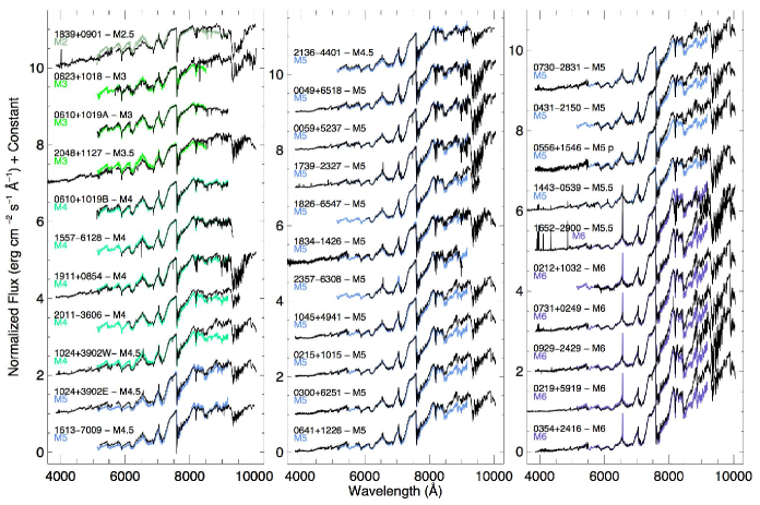
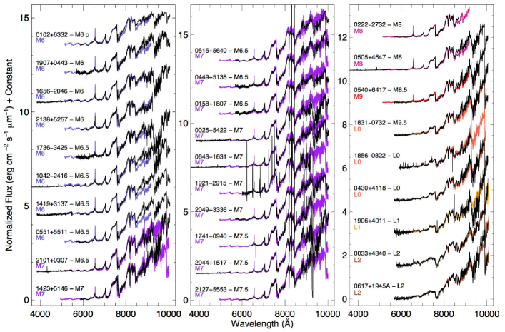
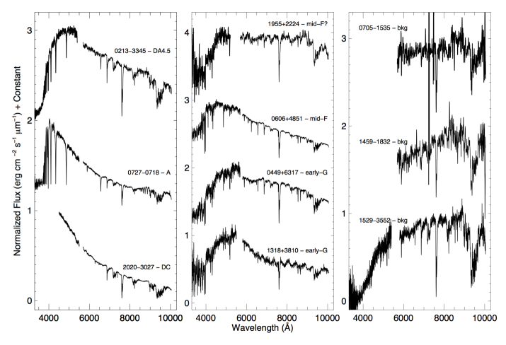
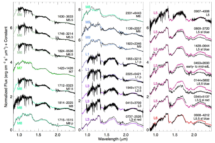
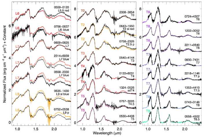
A.2.1 CTIO/RCSpec
Optical follow-up of five objects was obtained on the UT dates of 1995 August 13-14, 1997 July 14, and 1997 July 16 at the Cerro Tololo Interamerican Observatory (CTIO) 4m telescope and on 1996 May 20 at the CTIO 1.5m telescope using the R-C Spectrograph with Folded Schmidt Camera (RCSpec). For the 1995 and 1996 observations, a 300 line mm-1 grating with a GG 495 order-blocking filter was used with the 10241024 CCD to cover a wavelength range from 6050 to 9550 Å. For the 1997 observations, a 316 line mm-1 grating with an OG 515 order-blocking filter was used with the Loral 3K CCD to cover a useable wavelength range from 5200 to 10000 Å. In addition to the targets, standard calibrations – biases, dome flats, arcs, and flux calibration standards – were also obtained. Reductions were accomplished using the Image Reduction and Analysis Facility (IRAF; Tody 1986, 1993), as described in Kirkpatrick et al. (1997).
A.2.2 Lick/Kast
The Kast Double Spectrograph at the Lick 3m Shane Telescope was used for optical follow-up of six objects on UT dates 2019 September 20, 2020 March 06, 2020 August 15-16, 2020 December 14, and 2022 July 02. The only data used were from the red arm, which employed a 600 line mm-1 grating blazed at 7500 Å to cover the wavelength range from 6000 to 9000 Å. In addition to standard wavelength and flux calibrations, G2V and A0V stars were obtained near in time and on sky to the targets to correct for telluric absorption. The data were reduced using the kastredux474747https://github.com/aburgasser/kastredux package (Burgasser et al., in prep.), as further described in Schneider et al. (2021).
A.2.3 Palomar/DBSP
The Double Spectrograph (DBSP; Oke & Gunn 1982) at the Hale 5m telescope on Palomar Mountain was used for sixty additional follow-up spectra. The UT nights of observation were 1995 December 02, 2021 December 06, 2022 January 02, 2022 February 03, 2022 February 07, 2022 May 24, 2022 May 30, 2022 June 07, and 2022 August 27. For the 1995 run, the D68 dichroic was used to split the light at 6800 Å between the two arms. Gratings with 300 line mm-1 blazed at 3990 Å and with 316 line mm-1 blazed at 7150 Å were used in the blue and red arms, respectively, producing continuous wavelength coverage from 5100 to 9200 Å. For the 2021 and 2022 runs, the D55 dichroic was used instead to split the light near 5500 Å. A 600 line mm-1 grating blazed at 3780 Å was used in the blue arm and a 316 line mm-1 blazed at 7150 Å was used in the red arm, producing coverage from 3300 to 5500 Å on the blue side and from 5700 to 10000 Å on red side. (For the 2022 June run, fringing in the blue arm caused data shortward of 4500 Å to be unusable.) Standard calibrations and IRAF data reductions were employed, as further described in Kirkpatrick et al. (1991).
A.2.4 SALT/RSS
An additional optical spectrum was acquired with the Robert Stobie Spectrograph (RSS; Burgh et al. 2003; Kobulnicky et al. 2003) on the 11.19.8-m Southern African Large Telescope (SALT; Buckley et al. 2006) on 2021 December 26 UT. The spectrograph was used in long slit mode using the PG0900 grating at an angle of 20∘, which produces coverage over the ranges 6033-7028, 7079-8045, and 8091-9023 Å across the 31 mini-mosaic. Our reductions began with the observatory-provided pre-processed data, for which gain correction, correction for cross-talk, and overscan subtraction had been applied. We then wavelength calibrated using neon arc lines obtained immediately after the target’s spectroscopic data and flux calibrated using the Hamuy et al. (1994) standard EG21 acquired with the same spectroscopic setup on 2023 January 24 UT.
A.2.5 APO/TSpec
TripleSpec (Wilson et al. 2004) on the ARC 3.5m telescope at Apache Point Observatory was used for near-infrared follow-up of two objects on the nights of 2018 September 23 and 2019 October 08 UT. The spectrograph provides spectral coverage from 0.95 to 2.46 m across five spectral orders. Data were taken with the conventional near-infrared technique of nodded pairs to perform background/bias subtraction, and standard calibrations were also acquired, including quartz lamps for flat fielding and A0 stars for telluric correction and flux calibration. Wavelength calibration was accomplished using night sky lines. Data reduction used Tspectool484848http://www.apo.nmsu.edu/arc35m/Instruments/TRIPLESPEC/#7, a modified version of Spextool (Cushing et al. 2004) rewritten specifically for APO/TripleSpec.
A.2.6 CTIO/ARCoIRIS
Three objects were observed on the nights of 2018 April 02-03 UT using the Astronomy Research with the Cornell Infra Red Imaging Spectrograph (ARCoIRIS) at the 4m Victor Blanco telescope at CTIO. Spectra are acquired across six cross-dispersed orders covering 0.8 to 2.4 m at a resolving power of 3500. Science exposures were taken with AB nod positions along the slit, which has a fixed width of 11. Standard calibrations were acquired as discussed in Greco et al. (2019), and data were reduced using a modified version of the Spextool package (Cushing et al. 2004), which utilizes A0 stars for telluric correction and flux calibration following the methodology of Vacca et al. (2003).
A.2.7 IRTF/SpeX
The SpeX instrument on the NASA Infrared Telescope Facility (IRTF) was used for near-infrared spectroscopy of twenty-seven objects over the nights of 2018 June 16, 2018 November 25, 2019 January 23, 2019 March 16-17, 2020 October 30, 2020 November 25, 2021 May 31, 2021 June 30, 2021 September 11, 2021 October 23, 2022 January 09, 2022 January 19, 2022 February 12, 2022 February 21, 2022 March 07, and 2022 March 11 UT. Two different setups were employed. The first, used mainly for brighter targets, was a cross-dispersed mode that provides spectra over the range 0.9-2.4 m at a resolving power of . The second, used primarily for fainter targets, was the prism mode that provides spectra over the range 0.8-2.5 m at a resolving power of . As discussed in the subsections above, standard near-infrared calibrations were obtained, and data were reduced using Spextool (Cushing et al. 2004, Vacca et al. 2003).
A.2.8 Keck/NIRES
Three objects were observed over the nights of 2019 February 14, 2020 July 07, and 2021 February 24 UT using the Near-Infrared Echellette Spectrometer (NIRES; e.g., Wilson et al. 2004) at the 10m W. M. Keck II telescope. These data provided spectral coverage from 0.94 to 2.45 m. Setup and calibrations were identical to those described in Meisner et al. (2020b), and reductions used a modified version of Spextool (Cushing et al. 2004, Vacca et al. 2003).
A.2.9 Magellan/FIRE
The Folded-port Infrared Echellette spectrograph (FIRE; Simcoe et al. 2013) at the 6.5 m Walter Baade (Magellan I) telescope at Las Campanas Observatory was used to observe three objects over the nights of 2016 January 23, 2019 December 11, and 2020 February 18 UT. Observations were done in prism mode, which covers the range from 0.80 to 2.45 m. Standard calibrations were acquired, and data were reduced using the FIREHOSE pipeline, which is based on the MASE (Bochanski et al. 2009) and Spextool (Cushing et al. 2004, Vacca et al. 2003) packages.
A.2.10 Palomar/TSpec
Finally, seven near-infrared spectra were acquired with the Triple Spectrograph (TSpec; Herter et al. 2008) at Palomar Mountain’s 5m Hale telescope on the nights of 2018 April 28-29, 2018 October 17, and 2019 September 18 UT. Setup and calibrations were identical to those described in Kirkpatrick et al. 2011. As with many of the other near-infrared spectroscopic data sets discussed above, TSpec data were also reduced with a modified version of Spextool (Cushing et al. 2004, Vacca et al. 2003).
A.2.11 Analysis
Spectral classification was accomplished by comparing spectra of the target objects to established on-sky anchors for each integral spectral type. For the optical spectra, these anchor points were taken from Kirkpatrick et al. (1991) for objects of type mid-K through late-M and from Kirkpatrick et al. (1999) for L dwarfs (Figures 23-24). Optical classifications of objects earlier than type K (Figure 25) used spectral anchors taken from Gray & Corbally (2009). Near-infrared classification (Figures 26-27) for M dwarfs, L dwarfs, and early-T dwarfs used the anchors described in Kirkpatrick et al. (2010), with the rest of the T dwarf anchors coming from Burgasser et al. (2006). For more on the methodology employed for both optical and near-infrared classifications, see Kirkpatrick et al. (2010).
These classification anchors are generally old disk objects with metallicities similar to the Sun. In a few cases, described below, the target object failed to match an anchor spectrum because of anomalous features attributable to extreme youth, lower metallicity, or other reasons including unresolved binarity. These special cases are addressed further below:
CWISE J045334.34+203350.2: At -band, this object best matches the L5 standard, but there are clear discrepancies with the L5 standard across all wavelengths (Figure 26). The continuum of 0453+2033 is much flatter between 1.1 and 1.3 m, the FeH band at 0.99 m is much stronger, and the - and -band portions emit less flux relative to -band than does the standard. We find that the -band spectrum of 0453+2033 is a better match to 2MASS J17561080+2815238, which is typed in both the optical and the near-infrared as an sdL1 (Kirkpatrick et al. 2010, Zhang et al. 2018), in both the continuum shape and the strength of the FeH band. However, 0453+2033 has more flux at and relative to than does 2MASS J1756+2815, possibly indicating that the former is a slightly later subdwarf. Given that the set of anchors for the L subdwarf spectral sequence is still incomplete (Zhang et al. 2018), we tentatively classify this object as an early- to mid-sdL.
CWISE J055942.94012002.4: Of the spectra in Figures 26-27 that have a "red" or "slightly red" classification, only 05590120 has the triangular-shaped -band peak indicative of low gravity. Such low-gravity objects are necessarily young, as they have not yet contracted to their final radii. Using just the sky position and proper motion values (Table 2), as its parallax and radial velocity have not yet been measured, BANYAN (Bayesian Analysis for Nearby Young Associations; Gagné et al. 2018) gives the object an 80% chance of belonging to a known, young moving group – either the AB Doradus group or, less likely, the Pictoris group. If an AB Dor member, BANYAN predicts 463 pc with a radial velocity of 222 km s-1; if a Pic member, the predictions are d = 213 pc and RV = 192 km s-1. Using solely an vs. spectral type relation (Dupuy & Liu 2012), as advocated for young L dwarfs in Schneider et al. (2023), we estimate a distance of 28.8 pc for this L5.5 dwarf, based on a value of mag from the 2MASS All-Sky Point Source Catalog.
CWISE J075227.38+053802.6: We classify this object as L9 pec (Figure 27). The peculiarities stem from the two unusual absorption troughs at 1.63 and 1.67 m within the -band plateau and the unusual inflection near 2.21 m at -band. Such features are indicative of methane absorption, which should not be present shortward of 2.5 m in an L9 dwarf. As previous papers such as Burgasser (2007b), Burgasser et al. (2010b), and Bardalez Gagliuffi et al. (2014) have noted, such spectra may indicate the presence of an unresolved binary comprised of two morphologically distinct spectra – a non-methane M or L dwarf and a methane-rich T dwarf. If 0752+0538 represents such an unresolved binary, modeling (see section 4.5 of Kirkpatrick et al. 2016) suggests it is likely a late-L plus early-T composite system.
CWISE J075853.12232645.8: We classify this object as T2.5 pec (Figure 27). Although its -band peak matches both the T2 and T3 standards equally well, the -band flux is suppressed and the -band flux elevated relative to the standards. We find that a synthetic spectrum made up of components of types L8-L9 and T5-T6 fits the overall spectral shape slightly better than the single standards, suggesting perhaps that this object is an unresolved binary.
CWISE J132403.81052631.4: The width of the -band peak in this object best matches that of the T4 standard (Figure 27), but the fits at both shorter and longer wavelengths are much poorer. Specifically, the - and -band portions of 13240526 emit less flux relative to -band than does the standard, and the -band portion is notably flattened, an effect often ascribed to increased collision-induced absorption by H2. Moreover, the -band portion emits more flux relative to -band than does the standard. Elevated -band flux and suppressed -band flux are seen in a comparison of the sdT5.5 dwarf HIP 73786B (Figure 1 of Zhang et al. 2019) to standards of type T5 and T6, although the discrepancies are stronger in 13240526, and the latter also shows suppressed -band flux. In the case of HIP 73786, the system has a measured subsolar metallicity of [Fe/H] = (Murray et al. 2011) from the K5 V primary, suggesting that the metallicity of 13240526 is somewhat lower still. We classify 13240526 as sdT4.
CWISE J221859.41+114642.7: The width of this object’s -band peak is most similar to the T7 standard, but its - and -band flux peaks are suppressed, with the latter being noticeably flattened. As with 13240526 above, such features are typical of subdwarfs, although the suppression of the -band peak in 2218+1146 runs contrary to the trend seen in T subdwarfs of slightly earlier type. In the sdT8 WISE J200520.38+542433.9, a wide companion in the low-metallicity ([Fe/H] = ) Wolf 1130 system (Mace et al. 2013b), the -band peak is shifted notably to the blue – from 1.09 to 1.03 m – relative to the standards, an effect also seen in the isolated sdT6.5 dwarf ULAS J131610.28+075553.0 (Burningham et al. 2014). Our spectrum is too noisy in this region to determine whether the same effect is present in 2218+1146, so we classify this object as T7 pec pending further confirmation of its subdwarf status.
| Object | Coords | Instrument | Obs. Date | Observer | Opt. | NIR |
|---|---|---|---|---|---|---|
| (hhmmddmm) | (UT) | Code | Spec. Type | Spec. Typeaa Near-infrared spectral types of "sl. blue", "blue", "sl. red", and "red" refer to objects that are slightly ("sl.") or considerably bluer or redder in the - and -bands than the established spectral standard at that subtype, after the standard spectrum and target spectrum are overplotted at -band. Those listed as "pec" (peculiar) have spectral morphologies that fail to match the established standards and cannot be characterized as easily. See section 5.2 of Kirkpatrick et al. (2010) for more discussion. | ||
| (1) | (2) | (3) | (4) | (5) | (6) | (7) |
| 2MASS J00251602+5422547 | 0025+5422 | Palomar/DBSP | 2022 Aug 27 | S | M7 | |
| CWISER J003350.99+434010.6 | 0033+4340 | Palomar/DBSP | 2022 Jan 02 | E,L,S,T | L2 | |
| 2MASS J00492565+6518038 | 0049+6518 | Palomar/DBSP | 2022 Aug 27 | S | M5 | |
| WISE J005936.73+523719.0 | 0059+5237 | Palomar/DBSP | 2022 Aug 27 | S | M5 | |
| 1RXS J010228.1+633256 | 0102+6332 | Palomar/DBSP | 2022 Jan 02 | E,L,S,T | M6 pec | |
| CWISE J013343.58+803153.1 | 0133+8031 | APO/TSpec | 2019 Oct 08 | A,Q | T4 | |
| CWISE J014407.64+380255.6 | 0144+3802 | IRTF/SpeX | 2022 Jan 09 | C,F | L5.5 blue | |
| WISEA J015815.65+180713.7 | 0158+1807 | Palomar/DBSP | 2022 Feb 03 | S | M6.5 | |
| 2MASS J02124635+1032546 | 0212+1032 | Palomar/DBSP | 2022 Feb 03 | S | M6 | |
| LP 941-19 | 02133345 | Palomar/DBSP | 2021 Dec 06 | S | DA4.5 | |
| LP 469-205 | 0215+1015 | Palomar/DBSP | 2022 Feb 03 | S | M5 | |
| 2MASS J02195603+5919273 | 0219+5919 | Palomar/DBSP | 2021 Dec 06 | S | M6 | |
| 2MASS J022247672732349 | 02222732 | Palomar/DBSP | 2021 Dec 06 | S | M8 | |
| 2MASS J03000272+6251582 | 0300+6251 | Palomar/DBSP | 2022 Feb 03 | S | M5 | |
| CWISE J034547.29+513716.0 | 0345+5137 | IRTF/SpeX | 2021 Nov 25 | C,F,R | L5.5 sl. red | |
| LP 357-56 | 0354+2416 | Palomar/DBSP | 2022 Feb 03 | S | M6 | |
| 2MASS J04134574+3709087 | 0413+3709 | Palomar/TSpec | 2018 Oct 17 | U,V,W | L3 | |
| Gaia EDR3 180116295441149824 | 0430+4118 | Palomar/DBSP | 2021 Dec 06 | S | L0 | |
| LP 834-48 | 04312150 | Palomar/DBSP | 2022 Feb 07 | S | M5 | |
| 2MASS J04490464+5138412 | 0449+5138 | Palomar/DBSP | 2022 Feb 03 | S | M6.5 | |
| UCAC4 767-032810 | 0449+6317 | Palomar/DBSP | 2022 Jan 02 | E,L,S,T | early-G | |
| CWISE J045334.34+203350.2 | 0453+2033 | IRTF/SpeX | 2018 Oct 01 | K,Y,Z | early- to mid-sdL | |
| 2MASS J05053461+4648017 | 0505+4647 | Palomar/DBSP | 2021 Dec 06 | S | M8 | |
| NLTT 14748 | 0516+5640 | Palomar/DBSP | 2022 Feb 03 | S | M6.5 | |
| CWISE J053046.20+440849.2 | 0530+4408 | IRTF/SpeX | 2020 Nov 25 | C,F,R | T5 | |
| LSPM J0540+6417 | 0540+6417 | Palomar/DBSP | 2021 Dec 06 | S | M8.5 | |
| CWISE J054034.89+414401.7 | 0540+4144 | IRTF/SpeX | 2022 Jan 09 | C,F | T3 | |
| Gaia DR2 265201384281320448 | 0551+5511 | Palomar/DBSP | 2022 Feb 03 | S | M6.5 | |
| WISEA J055600.48+154559.3 | 0556+1546 | Palomar/DBSP | 2022 Feb 03 | S | M5 pec110556+1546: Spectrum shows slightly stronger CaH bands relative to the M5 standard, though not enough to warrant a d/sdM5 designation. | |
| CWISE J055816.67450233.4 | 05584502 | Magellan/FIRE | 2020 Feb 18 | D | T8.5 | |
| CWISE J055829.92233053.4 | 05582330 | IRTF/SpeX | 2019 Mar 16 | F | L7 blue | |
| CWISE J055942.94012002.4 | 05590120 | IRTF/SpeX | 2022 Jan 09 | F | L5.5 red | |
| TYC 3382-603-1 | 0606+4851 | Palomar/DBSP | 2022 Jan 02 | E,L,S,T | mid-F | |
| CWISE J060822.15421244.7 | 06084212 | Magellan/FIRE | 2016 Jan 23 | M | L5.5 sl. blue | |
| CWISE J060938.91+062513.2 | 0609+0625 | IRTF/SpeX | 2020 Oct 30 | C,F,R,X | L7 | |
| BD+10 1032A | 0610+1019A | Palomar/DBSP | 1995 Dec 02 | 5 | M3 | |
| BD+10 1032B | 0610+1019B | Palomar/DBSP | 1995 Dec 02 | 5 | M4 | |
| CWISE J061741.79+194512.8 A | 0617+1945A | Palomar/DBSP | 2021 Dec 06 | S | L2 | |
| Gaia EDR3 3330473222213987072 | 0623+1018 | Palomar/DBSP | 2021 Dec 06 | S | M3 | |
| CWISE J063513.64143029.4 | 06351430 | IRTF/SpeX | 2022 Jan 09 | F | L9 sl. blue | |
| UPM J0641+1226 | 0641+1226 | Palomar/DBSP | 2022 Feb 03 | S | M5 | |
| WISEA J064313.95+163143.6 | 0643+1631 | Palomar/DBSP | 2021 Dec 06 | S | M7 | |
| CWISE J064341.04+195039.3 | 0643+1950 | Magellan/FIRE | 2019 Dec 11 | G,K | T2 sl. red | |
| Gaia EDR3 2936126887218756736 | 07051535 | Palomar/DBSP | 2021 Dec 06 | S | bkg | |
| CWISE J072418.16+430717.3 | 0724+4307 | Keck/NIRES | 2019 Feb 14 | B,2 | T6 | |
| UCAC4 414-032626 | 07270718 | Palomar/DBSP | 2021 Dec 06 | S | A2207270718: See section 4.7 of Tremblay et al. (2020) for an assessment of the spectral type. The Gaia DR2 parallax, which has a large uncertainty relative to other objects of similar magnitude, must be erroneous. No parallax is given in Gaia DR3. This star must actually fall well outside 20 pc. | |
| UPM J07302831 | 07302831 | Palomar/DBSP | 2022 Feb 03 | S | M5 | |
| 2MASS J07312949+0249084 | 0731+0249 | Palomar/DBSP | 2022 Feb 03 | S | M6 | |
| CWISE J073748.86252613.0 | 07372526 | IRTF/SpeX | 2019 Jan 23 | F,H | L3 sl. red | |
| CWISE J074346.98+314603.4 | 0743+3146 | Keck/NIRES | 2021 Feb 24 | B,J,2 | T8 | |
| CWISE J075227.38+053802.6 | 0752+0538 | IRTF/SpeX | 2022 Jan 09 | F | L9 pec (composite) | |
| CWISE J075628.41063709.5 | 07560637 | CTIO/ARCoIRIS | 2018 Apr 03 | F | L6: blue | |
| CWISE J075744.48-300504.3 | 07573005 | IRTF/SpeX | 2022 Feb 12 | F,N,O,R | T4.5 | |
| CWISE J075853.12232645.8 | 07582326 | IRTF/SpeX | 2022 Feb 21 | F,O | T2.5 pec (composite?) | |
| CWISE J080940.43372003.7 | 08093720 | IRTF/SpeX | 2019 Mar 17 | F | L5 sl. blue | |
| CWISER J090720.27430856.7 | 09074308 | CTIO/ARCoIRIS | 2018 Apr 02 | F | L5 | |
| LP 846-7 | 09292429 | Palomar/DBSP | 2022 Feb 03 | S | M6 | |
| CWISE J093035.01743148.6 | 09307431 | CTIO/ARCoIRIS | 2018 Apr 03 | F | T7 | |
| LSPM J1024+3902W | 1024+3902W | Palomar/DBSP | 2022 Feb 03 | S | M4.5 | |
| LSPM J1024+3902E | 1024+3902E | Palomar/DBSP | 2022 Feb 03 | S | M4.5 | |
| LP 848-50 | 10422416 | Palomar/DBSP | 2021 Dec 06 | S | M6.5 | |
| NLTT 25223 | 1045+4941 | Palomar/DBSP | 2022 Feb 03 | S | M5 | |
| CWISE J113646.36+205733.9 | 1136+2057 | IRTF/SpeX | 2019 Jan 23 | F,H | M9: | |
| CWISE J120258.26+305233.3 | 1202+3052 | IRTF/SpeX | 2022 Mar 07 | C,O | T6 | |
| UCAC4 641-049451 | 1318+3810 | Palomar/DBSP | 2022 Jan 02 | E,L,S,T | early-G | |
| CWISE J132403.81052631.4 | 13240526 | IRTF/SpeX | 2022 Jan 19 | C,F | sdT4 | |
| CWISE J135338.04+441017.6 | 1353+4410 | IRTF/SpeX | 2022 Mar 11 | C,N,O | T7.5 | |
| 2MASS J14194617+3137094 | 1419+3137 | Palomar/DBSP | 2022 Feb 03 | S | M6.5 | |
| NLTT 37185 | 1423+5146 | Lick/Kast | 2022 Jul 02 | B,1,2 | M7331423+5146: Spectrum shows slightly stronger CaH bands relative to the M7 standard, though not enough to warrant a d/sdM7 designation. | |
| LP 440-17 | 1423+1426 | IRTF/SpeX | 2021 Jun 30 | 3 | M7 | |
| CWISE J142830.96064435.5 | 14280644 | IRTF/SpeX | 2019 Mar 16 | F | L5 sl. blue | |
| UCAC3 169-135909 | 14430539 | Palomar/DBSP | 2022 Feb 03 | S | M5.5 | |
| (ditto) | (ditto) | Palomar/DBSP | 2022 May 24 | S | M5.5 | |
| Gaia EDR3 6305165514134625024 | 14591832 | Palomar/DBSP | 2022 May 24 | S | bkg | |
| Gaia EDR3 6013647666939138688 | 15293552 | Palomar/DBSP | 2022 May 24 | S | bkg | |
| L 153-43 | 15576128 | CTIO 1.5m/RCSpec | 1996 May 20 | 5 | M4 | |
| L 74-208 | 16137009 | CTIO 4m/RCSpec | 1997 Jul 16 | 5 | M4.5 | |
| SCR J16303633 | 16303633 | Palomar/TSpec | 2018 Apr 28 | U,V | M5.5 | |
| 2MASS J165235152900186 | 16522900 | Palomar/DBSP | 2022 Aug 27 | S | M5.5 | |
| SCR J16562046 | 16562046 | Palomar/DBSP | 2022 Aug 27 | S | M6 | |
| DENIS J171204.4032328 | 17120323 | Palomar/TSpec | 2018 Apr 28 | U,V | M7.5 | |
| CWISER J171509.58151534.6 | 17151515 | IRTF/SpeX | 2019 Mar 16 | F | M8 pec | |
| Gaia DR2 4053559111471124608 | 17363425 | Palomar/DBSP | 2022 Aug 27 | S | M6.5 | |
| 2MASS J173924402327071 | 17392327 | Palomar/DBSP | 2022 Aug 27 | S | M5 | |
| NLTT 45285 | 1741+0940 | Lick/Kast | 2020 Mar 06 | B,J,2 | M7.5 | |
| SCR J17463214 | 17463214 | Palomar/TSpec | 2018 Apr 29 | U,V | M5.5 | |
| CWISE J181429.08202534.4 | 18142025 | IRTF/SpeX | 2021 May 31 | 3 | M8 | |
| WISEA J182423.61053653.6 | 18240536 | Palomar/TSpec | 2018 Apr 28 | U,V | M6.5 | |
| WT 562 | 18266547 | CTIO 4m/RCSpec | 1995 Aug 14 | 5 | M5 | |
| Gaia DR2 4159791176135290752 | 18310732 | Palomar/DBSP | 2022 May 30 | P | M9.5 | |
| UCAC4 378-124295 | 18341426 | Palomar/DBSP | 2022 May 30 | P | M5 | |
| Gaia EDR3 4479498508613790464 | 1839+0901 | Palomar/DBSP | 2022 Aug 27 | S | M2.5 | |
| CWISE J185608.94082257.6 | 18560822 | Lick/Kast | 2019 Sep 20 | J,1 | L0 | |
| WISEP J190648.47+401106.8 | 1906+4011 | Palomar/DBSP | 2022 Aug 27 | S | L1 | |
| NLTT 47423 | 1907+0443 | Palomar/DBSP | 2022 May 30 | P | M6 | |
| CWISE J191118.88+085456.3 | 1911+0854 | Palomar/DBSP | 2022 Aug 27 | S | M4 | |
| 2MASS J192129772915507 | 19212915 | Lick/Kast | 2020 Aug 16 | B | M7 | |
| CWISE J192351.88+234611.8 | 1923+2346 | IRTF/SpeX | 2021 Sep 11 | C,F,R | M9 | |
| CWISE J194929.61+171301.3 | 1949+1713 | APO/TSpec | 2018 Sep 23 | A | L2.5 | |
| Gaia DR2 2034222547248988032 | 1955+3215 | Palomar/TSpec | 2019 Sep 18 | U,V | L1 pec | |
| UCAC4 563-099325 | 1955+2224 | Palomar/DBSP | 2022 May 30 | P | mid-F? | |
| HD 191408 B | 20113606 | CTIO 4m/RCSpec | 1995 Aug 13 | 5 | M4 | |
| EC 201733036 | 20203027 | Palomar/DBSP | 2022 Jun 07 | S | DC | |
| LSPM J2044+1517 | 2044+1517 | Palomar/DBSP | 2022 Aug 27 | S | M7.5 | |
| G 25-4 | 2048+1127 | Palomar/DBSP | 2022 May 30 | P | M3.5 | |
| 2MASS J20492745+3336512 | 2049+3336 | Palomar/DBSP | 2022 May 30 | P | M7 | |
| MFL2000 J210104.18+030705.1 | 2101+0307 | Palomar/DBSP | 2022 Aug 27 | S | M6.5 | |
| 2MASS J21272531+5553150 | 2127+5553 | Lick/Kast | 2020 Aug 15 | B,J,1 | M7.5 | |
| UCAC4 230-189452 | 21364401 | CTIO 4m/RCSpec | 1997 Jul 14 | 5 | M4.5 | |
| 2MASS J21381698+5257188 | 2138+5257 | Lick/Kast | 2020 Dec 14 | B,I,J,1,2 | M6 | |
| CWISE J221113.55+054006.6 | 2211+0540 | IRTF/SpeX | 2021 Oct 23 | C,F | T6 | |
| CWISE J221859.41+114642.7 | 2218+1146 | Keck/NIRES | 2020 Jul 07 | B,I,J | T7 pec | |
| Gaia DR2 2206265777300448768 | 2225+6421 | Palomar/TSpec | 2019 Sep 18 | U,V | L1 pec | |
| CWISE J231403.13+693935.2 | 2314+6939 | IRTF/SpeX | 2018 Jun 16 | F | L7 blue | |
| CWISE J233135.66+644356.5 | 2331+6443 | IRTF/SpeX | 2018 Nov 25 | F | M8: | |
| CWISE J233819.49385421.2 | 23383854 | IRTF/SpeX | 2021 Sep 11 | C,F,R | T0 | |
| WISEA J235713.21630827.6 | 23576308 | SALT/RSS | 2021 Dec 26 | F | M5 |
Note. — Observer code: A = Katelyn Allers, B = Adam Burgasser, C = Emily Calamari, D = Adam Schneider, E = Peter Eisenhardt, F = Jacqueline Faherty, G = Daniella Bardalez Gagliuffi, H = Eileen Gonzales, I = Christopher Theissen, J = Roman Gerasimov, K = Rocio Kiman, L = Guodong Li, M = Jonathan Gagné, N = Dan Caselden, O = Les Hamlet, P = Thomas Connor, Q = Blake Pantoja, R = Austin Rothermich, S = Daniel Stern, T = Chao-Wei Tsai, U = Eric Mamajek, V = Federico Marocco, W = Jon Rees X = Jose I. Adorno, Y = Johanna Vos, Z = Mark Popinchalk, 1 = Christian Aganze, 2 = Chih-Chun Hsu, 3 = Richard Smart, 4 = Ryan Low, 5 = Davy Kirkpatrick.
A.3 Astrometry
Additional parallaxes have been measured as part of an ongoing ground-based program and through serendipitous imaging data found in the Spitzer Heritage Archive. These results are discussed further below.
A.3.1 NPARSEC results
Nearby objects continue to be targeted as part of the NTT PARallaxes of Southern Extremely Cool objects (NPARSEC) project, a long-term program (186.C-0756 with R. Smart, PI; 105.C-0781, 108.21XQ.0001, and 108.21XQ.002 with E. Costa, PI) using the infrared spectrograph and imaging camera Son OF ISAAC (SOFI; Moorwood et al. 1998) on the New Technology Telescope (NTT). The observational methodology and reduction procedures are identical to those discussed in Smart et al. (2013). For the eleven objects listed in Table 25, the new NPARSEC preliminary values have smaller uncertainties than previously published parallaxes. The table gives the object names, J2000 coordinates, mean epoch of observation, the absolute parallax, the correction applied to the relative parallax to convert to absolute, the proper motion values in Right Ascension and Declination, the total time baseline of the NTT observations, the number of reference stars used, and the total number of separate observational epochs.
Nine of the targets have absolute parallaxes greater than 50 mas, but for SDSS J163022.92+081822.0 and 2MASS J233123784718274, these better determined parallaxes have values below 50 mas, so we now exclude these three from the 20-pc census. We note, however, that these results are still considered preliminary and will be finalized once the NPARSEC program draws to a close.
| Object | RA | Dec | Epoch | Abs. | Baseline | # of | # of | |||
|---|---|---|---|---|---|---|---|---|---|---|
| Name | J2000 | J2000 | Corr. | Ref. | Obs. | |||||
| (deg) | (deg) | (mas) | (mas) | (mas yr-1) | (mas yr-1) | (yr) | Stars | |||
| (1) | (2) | (3) | (4) | (5) | (6) | (7) | (8) | (9) | (10) | (11) |
| 2MASS J04070885+1514565 | 61.787883 | 15.248440 | 2019.80 | 57.012.24 | 0.73 | 211.810.34 | -120.640.33 | 11.1 | 62 | 20 |
| 2MASS J051035244208146 | 77.647251 | -42.135453 | 2011.12 | 51.392.64 | 0.66 | 86.890.55 | 588.340.39 | 11.1 | 87 | 24 |
| WISEPA J054231.26162829.1 | 85.629759 | -16.473971 | 2019.79 | 63.261.65 | 0.68 | -216.970.29 | 297.020.35 | 12.1 | 93 | 29 |
| WISEPA J062720.07111428.8 | 96.840776 | -11.246393 | 2015.92 | 77.022.86 | 0.35 | -11.680.53 | -339.320.68 | 12.1 | 342 | 27 |
| 2MASS J072900023954043 | 112.247022 | -39.893729 | 2013.23 | 110.801.50 | 0.36 | -564.460.33 | 1694.630.31 | 12.1 | 394 | 29 |
| 2MASS J093935482448279 | 144.900600 | -24.812421 | 2016.22 | 189.802.68 | 0.64 | 569.650.60 | -1040.600.63 | 12.1 | 124 | 27 |
| SDSS J163022.92+081822.0 | 247.595321 | 8.305773 | 2013.33 | 41.762.79 | 0.46 | -60.810.84 | -104.310.98 | 7.0 | 107 | 19 |
| 2MASS J182835724849046 | 277.139127 | -48.803065 | 2013.33 | 86.912.34 | 0.39 | 230.080.72 | 88.500.58 | 10.9 | 503 | 22 |
| 2MASS J222828894310262 | 337.120937 | -43.175128 | 2011.86 | 95.602.23 | 0.62 | 97.980.42 | -306.910.46 | 11.0 | 31 | 19 |
| 2MASS J233123784718274 | 352.849548 | -47.307891 | 2012.58 | 49.004.23 | 0.44 | 73.010.70 | -64.370.69 | 11.0 | 18 | 19 |
| 2MASSI J2356547155310 | 359.226264 | -15.888962 | 2013.55 | 64.782.26 | 1.12 | -432.190.39 | -605.380.63 | 11.1 | 13 | 19 |
A.3.2 Spitzer results
CWISE J181125.34+665806.4 (hereafter 1811+6658; see Figure 28) is located only 1.2 degrees from the north ecliptic pole (NEP), and the area around the NEP was routinely observed by the Spitzer Space Telescope. As shown in Table 23, the location of 1811+6658 was observed repeatedly in post-cryogenic programs 10147 (PI: Bock) and 13153 (PI: Capak) in an attempt to explore the genesis of fluctuations in the extragalactic background light and to provide IRAC/ch1 and IRAC/ch2 data on touchstone fields that will be used by Euclid, Roman, and JWST to study galaxy growth during the epoch of reionization. The data in program 10147 cover the timeframe from May 2014 to Sep 2014, and those in program 13153 cover Feb 2017 to Feb 2019.
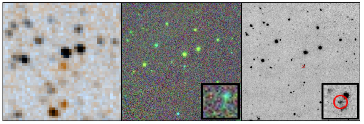
To extract astrometry from these data sets, we searched for blocks of ch2 coverage that had sufficient depth and redundancy to provide a similar per-epoch astrometric accuracy to that obtained in our own Spitzer parallax programs (Kirkpatrick et al. 2019, 2021a). (This cold brown dwarf is much brighter at ch2, 15.95 mag, than at ch1, 18.23 mag, so only the longer-wavelength band would provide sufficient signal-to-noise for our astrometric needs.) Program 10147 used 30s exposures per frame, and the position of 1811+6658 was observed at four or fewer epochs. The data from program 13153, on the other hand, used 100s exposures per frame and had more coverage at each sky position.
We pared this data set down to include only those frames for which the location of 1811+6658 was far enough from the frame edge to provide a reasonable number of Gaia DR3 reference stars surrounding the target’s location. Specifically, we retained only those ch2 frames that imaged all six of our pre-selected Gaia DR3 astrometric reference objects encircling a 60 zone centered on the location of 1811+6658. For program 10147, this left only two or three frames per epoch; this lack of redundancy combined with the short exposure time means that these data are unsuitable for astrometric analysis. For program 13153, however, we are left with four to six redundant, longer exposure frames per epoch (defined here to be per AOR), which is suitable for our reduction techniques. Of those program 13153 AORs listed in Table 23, only the ch2 data in 62377728, 65133312, 68615680, and 68631296 lacked sufficient redundancy. The time span covered by the remaining data sets is Jul 2017 to Jan 2019. These data were extracted and astrometrically calibrated to the Gaia DR3 reference frame as described in (Kirkpatrick et al. 2021a).
Given that the usable Spitzer data only cover a year and a half, we turned to WISE astrometry to provide the additional baseline needed to disentangle parallax from proper motion. The NEP is within the boresight of the WISE spacecraft on every orbit, but given the 47′-wide field of view, 1811+6658 is not within the continuous viewing zone. However, that location is viewed by WISE during a span of 50+ days every six months as the scan pattern rotates around the ecliptic pole. As such, there are several weeks of coverage twice per year covering its location.
We ran the crowdsource detection software (Schlafly et al. 2018) on time-resolved unWISE coadds (Meisner et al. 2018) for all ten-day epochal mosaics covering the position of 1811+6658. We retained those source lists for which the frame coverage depth at the location of 1811+6658 was 40 or greater. This was done in an effort to assure that the area surrounding the target’s location also had sufficient coverage, as this area is needed for the astrometric calibrators. The measured positions of these surrounding astrometric standards were used to place the measured position of 1811+6658 onto the same Gaia DR3 reference frame used for the Spitzer observations.
This astrometry from Spitzer and WISE is listed in Table 26. A fit to the parallax and proper motion was performed on the combined astrometry using the methodology outlined in Kirkpatrick et al. (2021a), resulting in the values shown in Table 27. The results of this fit are shown graphically in Figure 29. We find that the object has a distance of 14.3 pc and a value of mag. A comparison to Figure 16d of Kirkpatrick et al. (2021a) suggests a spectral type of early-Y for this absolute magnitude. We further note that the measured colors – ch2 = 5.660.04 mag, W1W2 = 3.040.09 mag, and ch1ch2 = 2.280.02 mag – suggest a slightly earlier spectral type of around T9-T9.5 based on Figures 16e, 16g, and 16h of Kirkpatrick et al. (2021a). A comparison of our Keck/MOSFIRE , and WISE W1+W2 images with data from PanSTARRS (Figure 28) shows that 1811+6658 is passing near two blue PanSTARRS sources. Given the low spatial resolution of the WISE (and Spitzer) data, we believe that our measurements of W1 (and ch1) are contaminated by these background objects. The higher resolution of the Keck/MOSFIRE data allows us to separate all three components, but our aperture photometry at is likely still compromised given our aperture radius of 6 pixels (). Therefore, our measured ch2, W1W2, and ch1ch2 color are all likely bluer than their true values, supporting our assertion of a Y dwarf spectral type.
| RA | Dec | Band | MJD | |||||
|---|---|---|---|---|---|---|---|---|
| (deg) | (deg) | (asec) | (asec) | (day) | (km) | (km) | (km) | |
| (1) | (2) | (3) | (4) | (5) | (6) | (7) | (8) | (9) |
| 272.8555557 | 66.9680473 | 0.01926 | 0.01576 | ch2 | 57951.3599612 | -146795664.394331 | -29137217.001001 | -15336117.968022 |
| 272.8554312 | 66.9680074 | 0.02229 | 0.02085 | ch2 | 58077.0419038 | 105457481.330533 | -102108810.219802 | -44432690.607376 |
| 272.8554058 | 66.9679956 | 0.02281 | 0.01313 | ch2 | 58122.9951224 | 153046661.423622 | -8618952.216674 | -1585273.269887 |
| 272.8554273 | 66.9679729 | 0.02411 | 0.01427 | ch2 | 58130.1216015 | 152890751.809545 | 7809001.342473 | 5815875.561150 |
| 272.8554284 | 66.9679740 | 0.01951 | 0.01134 | ch2 | 58137.7633120 | 150349854.612387 | 25297184.572655 | 13659004.961915 |
| 272.8554287 | 66.9679583 | 0.01908 | 0.02450 | ch2 | 58175.0395945 | 105086559.337856 | 99767940.252168 | 46540371.773800 |
Note. — (This table is available in its entirety in a machine-readable form in the online journal. A portion is shown here for guidance regarding its form and content.)
| Parameter | Value |
|---|---|
| (1) | (2) |
| RA at t0 | 272.855621 deg 33.5 mas |
| Dec at t0 | 66.968261 deg 28.7 mas |
| t0 (MJD) | 57293.81 |
| 69.76.8 mas | |
| 91.713.9 mas yr-1 | |
| 439.811.6 mas yr-1 | |
| 65.903 | |
| 129 | |
| 0.511 | |
| #Spitzer | 10 |
| #WISE | 57 |
| #Gaia | 6 |
Note. — The RA and Dec values are listed on the ICRS coordinate system. The last three rows represent the number of Spitzer ch2 epochs (#Spitzer) and the number of unWISE W2 epochs (#WISE) used in the fits, along with the number of five-parameter Gaia DR3 stars used for the astrometric re-registration (#Gaia).
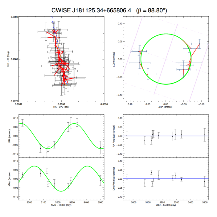
Appendix B The List of Proximal Systems
Despite recent WISE-based discoveries of the L+T dwarf binary system WISE J104915.57531906.1 AB (Luhman 2013; 1.99 pc distant) and the Y dwarf WISE J085510.83071442.5 (Luhman 2014; 2.28 pc distant) adding to our knowledge of the Sun’s immediate neighbors, Proxima Centauri (Innes 1915; 1.30 pc distant) remains the closest. It is often just referred to as "Proxima", Latin for "nearest", because it is the nearest to the Sun. Yet, its full name translates to "Nearest of Centaurus". This has led some curious individuals to wonder what are the nearest stars – i.e., the other proximal objects – of each of the other eighty-seven official constellations.
Table 3.1 allows us to answer this question, given our current knowledge of the 20-pc census. Proxima Centauri and its primary, Centauri AB, represent a rare multi-object system for which the parallaxes of the individual components are so accurate that we can determine the far-flung companion to be closer to us than its host binary. For other multi-object systems, discerning the closest component may be far more difficult. Using a short-period binary as an example, determining the closest object in the system depends upon the orbital period and orientation with respect to the Sun, as one component may be the closer one at some epochs and the more distant one at others. Hence, we will identify only the proximal systems in each constellation when a multi-object system arises.
Table 28 lists these proximal systems. As examples, the closest system in Canis Major is the binary Sirius AB, and the closest in Delphinus is the Y dwarf WISEPC J205628.90+145953.3. For several constellations, the proximal system is still ambiguous, given current uncertainties in the measured trigonometric parallaxes of the closest candidates. Constellations having two objects within 1 of the same closest value are indicated by footnotes. Note that all constellations have a proximal system within the 20-pc limit of Table 3.1, the most distant being the K dwarf HD 200779 at 15.05 pc, the closest known object in Equuleus.
| Constellation | Proximal System | Spectral Class | Parallax (mas) |
|---|---|---|---|
| (1) | (2) | (3) | (4) |
| And | Ross 248 | M | 316.48 |
| Ant | DENIS J104814.6395606 | M | 247.21 |
| Aps | L 43-72 AB | M+M | 85.71 |
| Aql | Altair ( Aql) | A | 194.95 |
| Aqr | EZ Aqr ABC | M+M+M | 289.50 |
| Ara | CD46 11540 | M | 219.64 |
| Ari | Teegarden’s Star | M | 260.98 |
| Aur | QY Aur AB | M+M | 165.21 |
| Boo | HD 119850 | M | 183.99 |
| Cae | L 374-6 | M | 70.06 |
| Cam | G 254-29 | M | 190.32 |
| Cap | LP 816-60 | M | 177.93 |
| Car | L 143-23 | M | 206.96 |
| Cas | Achird ( Cas AB) | F+K | 168.83 |
| Cen | Cen AB + Proxima Cen | G+K+M | 768.06 |
| Cep | HD 239960 AB | M+M | 249.96 |
| Cet | G 272-61 AB | M+M | 373.84 |
| Cha | SCR J11387721 | M | 119.34 |
| Cir | DENIS-P J1454078660447 | L | 93.94 |
| CMa | Sirius ( CMa AB) | A+wd | 79.21 |
| CMi | Procyon ( CMi AB) | F+wd | 284.56 |
| Cnc | G 51-15 | M | 279.24 |
| Col | AP Col | M | 115.39 |
| Com | Com | F | 108.72 |
| CrA | L 489-58 | M | 80.41 |
| CrB | LSPM J1524+2925 | M | 76.46 |
| Crt | CD23 9765 | M | 92.80 |
| Cru | L 194-11 | M | 76.35 |
| Crv | Ross 695 | M | 112.67 |
| CVn | Chara ( CVn) | G | 118.02 |
| Cyg | 61 Cyg AB | K+K | 286.00 |
| Del | WISEPC J205628.90+145953.3 | Y | 140.80 |
| Dor | L 230-188 | M | 140.69 |
| Dra | HD 173739 + HD 173740 | M+M | 283.84 |
| Equ | HD 200779 | K | 66.46 |
| Eri | Ran ( Eri) | K | 310.57 |
| For | LP 944-20 | M | 155.59 |
| Gem | HD 265866 | M | 179.06 |
| Gru | HD 204961 | M | 201.32 |
| Her | WISEPA J174124.26+255319.5 | T | 214.30 |
| Hor | L 372-58 | M | 272.16 |
| Hya | WISE J085510.83071442.5 | Y | 439.00 |
| Hyi | Hyi | G | 133.71 |
| Ind | Ind ABC | K+T+T | 274.84 |
| Lac | EV Lac | M | 197.95 |
| Leo | Wolf 359 | M | 415.17 |
| Lep | Gl 229 AB | M+T | 173.69 |
| Lib | Gl 570 ABCD | K+M+M+T | 170.01 |
| LMi | G 119-36 | M | 102.75 |
| Lup | CD40 9712 | M | 168.99 |
| Lyn | G 111-47 | M | 112.99 |
| Lyr | 2MASSI J1835379+325954 | M | 175.79 |
| Men | L 32-8 + L 32-9 | M+M | 113.13 |
| Mic | AX Mic | M | 251.91 |
| Mon | Ross 614 ABaaThe T dwarf UGPS J072227.51054031.2 is equidistant with this source within the measurement uncertainties. | M+M | 242.96 |
| Mus | LAWD 37 | wd | 215.67 |
| Nor | WISEA J154045.67510139.3 | M | 187.72 |
| Oct | L 49-19 | M | 116.31 |
| Oph | Barnard’s Star | M | 546.97 |
| Ori | G 99-49 | M | 192.01 |
| Pav | SCR J18456357 AB | M+T | 249.91 |
| Peg | WISE J220905.73+271143.9bbThe M dwarf pair BD+19 5116AB is equidistant with this source within the measurement uncertainties. | Y | 161.70 |
| Per | 2MASS J04195212+4233304ccThe T dwarf WISE J043052.92+463331.6 is equidistant with this source within the measurement uncertainties. | M | 97.44 |
| Phe | LAWD 96 | wd | 120.01 |
| Pic | Kapteyn’s Star | M | 254.19 |
| PsA | HD 217987 | M | 304.13 |
| Psc | Wolf 28 | wd | 231.78 |
| Pup | 2MASS J072900023954043ddThe M dwarf SCR J07404257 is equidistant with this source within the measurement uncertainties. | T | 126.30 |
| Pyx | CD32 5613 | wd | 117.39 |
| Ret | WISE J035000.32565830.2 | Y | 176.40 |
| Scl | HD 225213 | M | 230.09 |
| Sco | CD44 11909 | M | 199.69 |
| Sct | WISEA J182423.61053653.6 | M | 75.67 |
| Ser | HD 165222 | M | 129.21 |
| Sex | LP 731-58 | M | 219.33 |
| Sge | HD 349726 + Ross 730 | M+M | 113.25 |
| Sgr | Ross 154 | M | 336.02 |
| Tau | WISEPA J041022.71+150248.5 | Y | 151.30 |
| Tel | L 347-14 | M | 169.23 |
| TrA | WISE J163940.86684744.6 | Y | 219.60 |
| Tri | LP 245-10 | M | 96.73 |
| Tuc | CD68 47 | M | 121.44 |
| UMa | Lalande 21185 | M | 392.75 |
| UMi | WISEPC J150649.97+702736.0 | T | 193.94 |
| Vel | WISE J104915.57531906.1AB | L+T | 501.55 |
| Vir | Ross 128 | M | 296.30 |
| Vol | LAWD 26 | wd | 122.41 |
| Vul | WISE J192841.35+235604.9 | T | 146.40 |
It is worth noting the prevalence of brown dwarfs in Table 28. There are four T dwarf companions residing in proximal systems with K or M dwarf primaries, one L+T binary as its own proximal system, and eleven solivagant L, T, or Y dwarfs that are proximal objects in their own right. In this latter group, over half (six) of the these are Y dwarfs, a spectral type that is not yet fully sampled near the Sun.