Compact moduli of Enriques surfaces with a numerical polarization of degree 2

Abstract.

We describe a geometric, stable pair compactification of the moduli space of Enriques surfaces with a numerical polarization of degree $2$, and identify it with a semitoroidal compactification of the period space.

1. Introduction

Enriques surfaces are quotients of K3 surfaces by basepoint free involutions. They satisfy $2K\sim 0$ and $q=0$ and occupy a place somewhere in between rational and K3 surfaces. Unlike K3 surfaces, there are only finitely many moduli spaces of polarized Enriques surfaces, see [GH16]. Each of them parameterizes the same surfaces, with some finite data attached.

In this paper we consider the moduli space $F_{\rm En,2}$ of pairs $(Z,[{\mathcal{L}}_{Z}])$, where $Z$ is an Enriques surface with $ADE$ singularities and $[{\mathcal{L}}_{Z}]\in\operatorname{Pic}Z/{\mathbb{Z}}_{2}$ is an ample numerical polarization of degree $2$. Equivalently, this is the moduli space of $ADE$ Enriques surfaces $(Z,{\mathcal{M}})$ with a $2$-divisible polarization ${\mathcal{M}}={\mathcal{L}}_{Z}^{\otimes 2}\in\operatorname{Pic}Z$ of degree $8$. The Baily-Borel compactification ${\overline{F}}_{\rm En,2}^{\rm BB}$ of this space was described by Sterk [Ste91].

By the classification of big and nef linear system on Enriques surfaces [Cos83], see also [CD89, CDL24], the linear system $|{\mathcal{M}}|$ is basepoint free and defines a double cover $\rho\colon Z\to W$ to a quartic del Pezzo surface with $4A_{1}$ or $A_{3}+2A_{1}$ singularities. The ramification divisor $R_{Z}\in|{\mathcal{M}}|$ of $\rho$ is ample and the pair $(Z,\epsilon R_{Z})$ is log canonical for any $0<\epsilon\ll 1$. Thus, the moduli space $F_{\rm En,2}$ admits a geometric, modular compactification ${\overline{F}}_{\rm En,2}$ in the KSBA moduli space of pairs $(Z,\epsilon R_{Z})$ with semi log canonical singularities, $K_{Z}\equiv 0$ and ample ${\mathbb{Q}}$-Cartier divisor $R_{Z}$. See [Kol23] for their general theory. Our main result, in Section 5.2, is

Theorem 1.1.

The normalization of ${\overline{F}}_{\rm En,2}$ is a semitoroidal compactification ${\overline{F}}_{\rm En,2}^{\mathfrak{F}}$ corresponding to a collection ${\mathfrak{F}}=\{{\mathfrak{F}}^{k}\}_{k=1,2,3,4,5}$ of explicit semifans, one for each $0$-cusp of $F_{\rm En,2}$, and it is dominated by a toroidal compactification ${\overline{F}}_{\rm En,2}^{\rm cox}$ for a collection ${\mathfrak{F}}_{\rm cox}=\{{\mathfrak{F}}^{k}_{\rm cox}\}_{k=1,2,3,4,5}$ of Coxeter fans.

In Sections 6, 7 we describe all stable pairs parametrized by the boundary of ${\overline{F}}_{\rm En,2}$. The irreducible components of these pairs turn out to be surfaces that naturally correspond to the ABCDE Dynkin diagrams. They generalize the ADE surfaces of [AT21] that appear on the boundary of K3 moduli spaces.

In Section 4 we also provide a detailed description of some nice models of Enriques degenerations, which are slightly more singular than simple normal crossing. Instead, they are dlt (divisorially log terminal, see [KM98, Def. 2.37]).

Just as weighted graphs encode semistable degenerations of curves, $K$-trivial semistable (i.e. Kulikov) degenerations of K3 surfaces ${\mathcal{X}}\to(C,0)$ are encoded by integral-affine structures on the $2$-sphere, or $\operatorname{IAS^{2}}$ [GHK15a, Eng18, EF21]. An $\operatorname{IAS^{2}}$ is a collection of local embeddings of $S^{2}$ minus a finite set into the flat plane, which differ on overlaps by $\operatorname{SL}_{2}({\mathbb{Z}})\ltimes{\mathbb{Z}}^{2}$. Complete triangulations of $\operatorname{IAS^{2}}$ which take their vertices in ${\mathbb{Z}}^{2}$, under the local embedding, describe the dual complexes $\Gamma({\mathcal{X}}_{0})$ of Kulikov degenerations. In this paper, we realize Diagram (1) on the integral-affine level, by constructing $\Gamma({\mathcal{X}}_{0})$ together with two commuting involutions $\iota_{{\rm En},\,{\rm IA}}$ and $\iota_{{\rm dP},{\rm IA}}$ of the $\operatorname{IAS^{2}}$.

The quotient of $\Gamma({\mathcal{X}}_{0})$ by $\iota_{{\rm En},\,{\rm IA}}$ is either an integral-affine structure on a disk ${\mathbb{D}}^{2}$ or a real-projective plane ${\mathbb{R}}{\mathbb{P}}^{2}$. These ${\rm IA}{\mathbb{D}}^{2}$ and ${\rm IA}{\mathbb{R}}{\mathbb{P}}^{2}$ are the dual complexes $\Gamma({\mathcal{Z}}_{0})$ of particularly nice dlt models of Enriques surface degenerations ${\mathcal{Z}}\to(C,0)$. From these dlt models, one can extract a completely explicit description of the stable limit of any degeneration in ${\overline{F}}_{\rm En,2}$ from Hodge-theoretic data.

The validity of our description of these Kulikov, dlt, and stable models relies on the general theory of compactifications of moduli spaces of K3 surfaces developed by the first two authors [AE23, AE22]. Most relevant to the situation at hand, [AE22] considers the $75$ moduli spaces of K3 surfaces with a non-symplectic involution. For $50$ of them, the ramification divisor $R$ contains a component $C$ of genus $g(C)\geq 2$ providing a polarization. For these, [AE22] describes the Kulikov models and KSBA compactification for the pairs $(X,\epsilon C)$.

Crucial for us here is the compactified moduli space ${\overline{F}}_{(2,2,0)}$ of K3 surfaces of degree $4$ with a del Pezzo involution $\iota_{{\rm dP}}$ corresponding, generically, to double covers of ${\mathbb{P}}^{1}\times{\mathbb{P}}^{1}$ branched over a curve of bidegree $(4,4)$. By immersing the moduli space ${\overline{F}}_{\rm En,2}\to{\overline{F}}_{(2,2,0)}$ and understanding the Enriques involution on the fibers, we give a description of ${\overline{F}}_{\rm En,2}$ and its universal family.

The plan of the paper is as follows. In Section 2 we discuss the model of Enriques surfaces which we use in this paper. We also recall the description of the moduli space $F_{\rm En,2}$ after Sterk [Ste91]. Then we describe morphisms between $F_{\rm En,2}$, $F_{(2,2,0)}$ and the moduli $F_{(10,10,0)}$ of unpolarized Enriques surfaces. Finally, we briefly recall the theory of KSBA stable pairs and their compact moduli.

In Section 3 we recall the cusp diagrams of $F_{(2,2,0)}$, $F_{(10,10,0)}$, $F_{\rm En,2}$ and determine how they map to each other. Next, we describe Coxeter diagrams associated to each of the five $0$-cusps and the $9$ $1$-cusps of $F_{\rm En,2}$. The diagrams are the same as in Sterk [Ste91] but we find them in a different way, “folding by involutions” the Coxeter diagrams of the lattices $U\oplus E_{8}^{2}$ and $U(2)\oplus E_{8}^{2}$ corresponding to the two $0$-cusps of $F_{(2,2,0)}$. This is the combinatorial heart of the paper. An idea from [AET23, AE22] employed here is that one can read off degenerations of K3 surfaces directly from Coxeter diagrams. Consequently, we are able to read off degenerations of Enriques surfaces from the Coxeter diagrams of $F_{\rm En,2}$.

Using the above description, in Section 4 we find integral-affine spheres with two commuting involutions $\iota_{{\rm En},\,{\rm IA}}$ and $\iota_{{\rm dP},{\rm IA}}$ and the corresponding Kulikov models of K3 surfaces with involutions. We then describe how to construct the dlt models for degenerations of Enriques surfaces, and give some detailed examples.

In Section 5, as an application of general theory and in a similar way to [ABE22, AE22] we describe the KSBA compactification ${\overline{F}}_{\rm En,2}$ and the stable pairs appearing on the boundary. For K3 surfaces, the irreducible components of degenerations are ADE surfaces of [AT21]. In the case of Enriques surfaces, additional B and C surfaces appear, corresponding to $B$ and $C$ Dynkin diagrams resulting from folding ADE diagrams. We describe them in Sections 6 and 7.

We work over the complex numbers, although most of the results can be generalized to any field of characteristic $\neq 2$.

Acknowledgements.

The first author was partially supported by the NSF under DMS-2201222. The second author was partially supported by the NSF under DMS-2201221. The fourth author is a member of the INdAM group GNSAGA and was partially supported by the projects “Programma per Giovani Ricercatori Rita Levi Montalcini”, PRIN2020KKWT53 and PRIN 2022 – CUP E53D23005790006.

We thank Igor Dolgachev for helpful comments.

2. General setup

2.1. The main diagram, general case

Consider a surface $Y={\mathbb{P}}^{1}\times{\mathbb{P}}^{1}$ with an involution $\tau\colon(x,y)\to(-x,-y)$ and quotient $W=Y/\tau$. Let $B\in|-2K_{Y}|$ be a $\tau$-invariant divisor with at worst $ADE$ singularities not passing through the four points with $x,y\in\{0,\infty\}$ fixed by $\tau$. The double cover $\pi\colon X\to Y$ branched in $B$ is a K3 surface with a del Pezzo involution $\iota_{{\rm dP}}$ so that $Y=X/\iota_{{\rm dP}}$. The involution $\tau$ on $Y$ lifts to a basepoint-free Enriques involution $\iota_{{\rm En}}$ on $X$ commuting with $\iota_{{\rm dP}}$ and the quotient $Z=X/\iota_{{\rm En}}$ is an Enriques surface. The second lift of $\tau$ is a Nikulin involution and the quotient $Z^{\prime}=X/\iota_{{\rm Nik}}$ is a K3 surface with eight $A_{1}$ singularities and possibly more. This gives the following commutative diagram:

(1)

The surface $Y={\mathbb{P}}^{1}\times{\mathbb{P}}^{1}$ is toric and the line bundle ${\mathcal{O}}(4,4)$ has, as its polytope, a square $Q$ with sides of lattice length $4$, shown in the left panel of Figure 1. The surface $W$ is toric as well, for the same polytope but for the even sublattice ${\mathbb{Z}}^{2}_{{\rm ev}}=\{(a,b)\mid a+b\in 2{\mathbb{Z}}\}$ shown by gray dots. It is a quartic del Pezzo surface with four $A_{1}$ singularities. Vectors in ${\mathbb{Z}}^{2}_{{\rm ev}}$ are in bijection with monomials $x^{a}y^{b}$ invariant under the involution $\tau\colon(x,y)\to(-x,-y)$. Here, we freely identify monomials $1,x,\dotsc x^{4}$ with $x_{0}^{4},x_{0}^{3}x_{1},\dotsc,x_{1}^{4}$, and $1,y,\dotsc,y^{4}$ with $y_{0}^{4},y_{0}^{3}y_{1},\dotsc,y_{1}^{4}$.

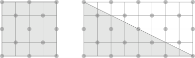
Figure 1. Polytopes $Q$ and lattices for the toric surfaces $Y$ and $W$

Let $f(x,y)$ be a $\tau$-invariant polynomial of bidegree $(4,4)$ in which $1$, $x^{4}$, $y^{4}$, $x^{4}y^{4}$ have nonzero coefficients, so that the hypersurface $\{f(x,y)=0\}\subset Y=V_{Q}$ does not contain any of the four torus-fixed points. Let $P\subset{\mathbb{R}}^{3}$ be the pyramid over $Q\subset 0\times{\mathbb{R}}^{2}$ with the vertex $(2,2,2)$, to which we associate the monomial $z^{2}$. Then the K3 surface $X$ is a hypersurface defined by the equation $z^{2}+f(x,y)$ in the projective toric variety $V_{P}$ associated with $P$. The polynomials $f(x,y)$ invariant under $\tau$ are linear combinations of $13$ monomials marked by gray dots. Thus, $f$ defines a point in an open subset $U\subset{\mathbb{P}}^{12}$ and in its quotient $U/D_{4}\ltimes({\mathbb{C}}^{*})^{2}$, of dimension $10$. There are three commuting involutions on $X$:

del Pezzo $$\iota_{{\rm dP}}\colon(x,y,z)\to(x,y,-z)$$

Enriques $$\iota_{{\rm En}}\colon(x,y,z)\to(-x,-y,-z)$$

Nikulin $$\iota_{{\rm Nik}}\colon(x,y,z)\to(-x,-y,z)$$

which together with the identity form a Klein-four group. Both $\iota_{{\rm En}}$ and $\iota_{{\rm Nik}}$ are lifts of $\tau$. On an affine subset of $X$ a nonvanishing $2$-form is given by

$$\omega=\operatorname{Res}_{X}\frac{dx\wedge dy\wedge dz}{z^{2}+f}.$$

One has $\iota_{{\rm dP}}^{*}\omega=\iota_{{\rm En}}^{*}\omega=-\omega$ and $\iota_{{\rm Nik}}^{*}\omega=\omega$. So $\iota_{{\rm dP}}$ and $\iota_{{\rm En}}$ are nonsymplectic and $\iota_{{\rm Nik}}$ is symplectic. The Enriques surface $Z$ is then a hypersurface in the toric variety for the polytope $P$ but for the even sublattice ${\mathbb{Z}}^{3}_{{\rm ev}}=\{(a,b,c)\mid a+b+c\in 2{\mathbb{Z}}\}$. It is defined by the same polynomial $z^{2}+f(x,y)$ whose monomials lie in ${\mathbb{Z}}^{3}_{{\rm ev}}$.

Let $R$ be the ramification divisor of $\pi$. The involution $\iota_{{\rm dP}}$ on $X$ descends to an involution $\tau_{{\rm dP}}$ on $Z$, and $W=Z/\tau_{{\rm dP}}$. Let $R_{Z}$ and $B_{W}$ be the ramification and branch divisors of $\rho$. Then $R=\psi^{*}(R_{Z})$ and $R_{Z}=\frac{1}{2}\psi_{*}(R)$. Since $R=\frac{1}{2}\pi^{*}(B)$ is an ample divisor, $R_{Z}$ is ample as well. One has ${\mathcal{O}}(R_{Z})={\mathcal{L}}_{Z}^{\otimes 2}\in\operatorname{Pic}Z$.

Horikawa [Hor78b] analyzed in some detail the sets of possible equations $f(x,y)$ and the maps from various opens subsets of ${\mathbb{P}}^{12}$ to the period domain ${\mathbb{D}}/\Gamma$ and its Baily-Borel compactification, introduced in the next section. In particular, he showed that certain mildly singular $f(x,y)$ vanishing at a torus-fixed point correspond to Coble surfaces, which are $S_{2}$-quotients of nodal K3 surfaces.

The GIT compactification ${\mathbb{P}}^{12}/\!/D_{4}\ltimes({\mathbb{C}}^{*})^{2}$ was described by Shah [Sha81], who gave normal forms for polystable orbits. As usual for the moduli of K3 surfaces with a projective construction, the relation between the GIT and the Baily-Borel compactifications is not straightforward, cf. [Loo86] for K3 surfaces of degree $2$ and [LO21] for degree $4$ K3 surfaces which are double covers of ${\mathbb{P}}^{1}\times{\mathbb{P}}^{1}$.

2.2. The main diagram, special case

The previous section describes the general case, when the K3 cover $X$ is non-unigonal. The special case corresponds to a Heegner divisor in $F_{\rm En,2}$ for which $(Y,L)=({\mathbb{P}}(1,1,2),{\mathcal{O}}(4))$ is a singular quadric. The toric surfaces $Y$ and $W$ correspond to the same polytope $Q$ shown in the right panel of Figure 1 but for different lattices: ${\mathbb{Z}}^{2}$ and ${\mathbb{Z}}^{2}_{{\rm ev}}$. The surface $W$ is a quartic del Pezzo surface with $A_{3}+2A_{1}$ singularities.

There are still $13$ even monomials giving a family over $U\subset{\mathbb{P}}^{12}$. However, in this case $\operatorname{Aut}(W)$, the centralizer of $\tau$ in $\operatorname{Aut}(Y)$, is three-dimensional, equal to $S_{2}\ltimes({\mathbb{C}}^{*}{}^{2}\ltimes{\mathbb{C}})$. So there is only a $9$-dimensional family of non-isomorphic surfaces.

Remark 2.1.

To our knowledge, Diagram (1) minus $Z^{\prime}$ first appeared in [Cos83, 6.3.1], see also [CD89, Cor. 4.7.2]. Horikawa model [Hor78a] is a birationally isomorphic version of this diagram. Ultimately, it can be traced back to the Enriques’ double plane model [Enr06]. We refer the reader to [CDL24] for a detailed historical account and many other projective models of Enriques surfaces.

Remark 2.2.

The entire Diagram (1) is intrinsic to the pair $(Z,[{\mathcal{L}}_{Z}])$, in both the general and special cases. Indeed, $W=\varphi_{|{\mathcal{L}}_{Z}^{\otimes 2}|}(Z)$, $Y=\operatorname{Spec}{\mathcal{O}}_{W}\otimes{\mathcal{O}}_{W}(A)$ where $A$ is the generator of $\operatorname{Tors}\operatorname{Cl}(W)={\mathbb{Z}}_{2}$, and $X=Y\times_{W}Z$. One has

$$Z^{\prime}=\operatorname{Spec}{\mathcal{O}}_{W}\oplus{\mathcal{O}}_{W}(K_{W})\quad\text{and}\quad Z=\operatorname{Spec}{\mathcal{O}}_{W}\oplus{\mathcal{O}}_{W}(K_{W}+A)$$

with the multiplications defined by the divisor $B_{W}\in|-2K_{W}|=|-2(K_{W}+A)|$.

2.3. Period domains

We follow [Ste91] for the moduli space of Enriques surfaces with a numerical degree $2$ polarization, and [AE22] for the moduli space of K3 surfaces of degree $4$ with a nonsymplectic involution.

Let $L=I\!I_{3,19}=U^{3}\oplus E_{8}^{2}\simeq H^{2}(X,{\mathbb{Z}})$ be the K3 lattice. It is even, unimodular and has signature $(3,19)$. Here, $U=I\!I_{1,1}$ and our $E_{8}=I\!I_{0,8}$ is a negative-definite unimodular lattice. Let us write $L$ in block form:

$$L=U\oplus U\oplus U\oplus E_{8}\oplus E_{8}=\{(v,u,u^{\prime},e,e^{\prime})\mid v,u,u^{\prime}\in U,\ e,e^{\prime}\in E_{8}\}$$

Definition 2.3.

Define three involutions $I_{\rm dP}$, $I_{\rm En}$ and $I_{\rm Nik}=I_{\rm dP}\circ I_{\rm En}$ on $L$ corresponding to the Enriques, del Pezzo, and Nikulin involutions on K3 surfaces of degree $4$ as follows (cf. [PS20] for the nodal case):

$$I_{\rm dP}\colon (v,u,u^{\prime},e,e^{\prime})\to(-v,u^{\prime},u,-e,-e^{\prime})$$

$$I_{\rm En}\colon (v,u,u^{\prime},e,e^{\prime})\to(-v,u^{\prime},u,e^{\prime},e)$$

$$I_{\rm Nik}\colon (v,u,u^{\prime},e,e^{\prime})\to(v,u,u^{\prime},-e^{\prime},-e)$$

Their $(\pm 1)$-eigenspaces are

$$S_{\rm dP}:=L_{\rm dP}^{+}=\Delta(U)\quad T_{\rm dP}:=L_{\rm dP}^{-}=U\oplus\Delta^{-}(U)\oplus E_{8}^{2}$$

$$S_{\rm En}:=L_{\rm En}^{+}=\Delta(U)\oplus\Delta(E_{8})\quad T_{\rm En}:=L_{\rm En}^{-}=U\oplus\Delta^{-}(U)\oplus\Delta^{-}(E_{8})$$

$$L_{\rm Nik}^{+}=U^{3}\oplus\Delta^{-}(E_{8}) L_{\rm Nik}^{-}=\Delta(E_{8})$$

Here, $\Delta$ and $\Delta^{-}$ denote the diagonals and anti-diagonals in $U^{2}$ and $E_{8}^{2}$. As lattices, they are isomorphic to

$$S_{\rm dP}=U(2)=(2,2,0)_{1}\quad T_{\rm dP}=U\oplus U(2)\oplus E_{8}^{2}=(20,2,0)_{2}$$

$$S_{\rm En}=U(2)\oplus E_{8}(2)=(10,10,0)_{1}\quad T_{\rm En}=U\oplus U(2)\oplus E_{8}(2)=(12,10,0)_{2}$$

$$L_{\rm Nik}^{+}=U^{3}\oplus E_{8}(2)=(14,8,0)_{3} L_{\rm Nik}^{-}=E_{8}(2)=(8,8,0)_{0}$$

All these lattices are even and $2$-elementary, i.e. with the discriminant group $\Lambda^{*}/\Lambda\simeq{\mathbb{Z}}_{2}^{a}$ for some $a$. Recall, see e.g. [Nik79], that an indefinite even $2$-elementary lattice is uniquely determined by its signature and a triple $(r,a,\delta)$, where $r=\operatorname{rk}_{\mathbb{Z}}(\Lambda)$, $a=\operatorname{rk}_{{\mathbb{Z}}_{2}}(\Lambda^{*}/\Lambda)$ and $\delta\in\{0,1\}$ is the coparity: $\delta=0$ if the discriminant form $q_{\Lambda}\colon\Lambda^{*}/\Lambda\to\frac{1}{2}{\mathbb{Z}}/2{\mathbb{Z}}$, $q_{\Lambda}(x)=x^{2}{\ \rm mod\ }2{\mathbb{Z}}$ is ${\mathbb{Z}}$-valued and $\delta=1$ otherwise. In our notation, $(r,a,\delta)_{n_{+}}$ denotes such a lattice of signature $(n_{+},n_{-})$.

Lemma 2.4.

The sequence $U\oplus U(2)\oplus E_{8}(2)\to U\oplus U(2)\oplus E_{8}^{2}\to L$ of primitive embeddings is unique up to an isometry in $O(L)$.

Proof.

By taking the orthogonals, this is equivalent to the condition that the sequence of primitive embeddings $U(2)\to U(2)\oplus E_{8}(2)\to L$ is unique. The second embedding is unique by [Nik79, 1.14.4]. The first embedding is equivalent to the embedding $U\to\Lambda=U\oplus E_{8}$ and it is well known that it is unique. Indeed, $\Lambda=U\oplus U^{\perp}$ and $U^{\perp}\simeq E_{8}$. The homomorphisms $O(L)\to O(T_{\rm dP})$ and $O(L)\to O(T_{\rm En})$ are surjective by [Nik79, 1.5.2, 3.6.3]. ∎

Definition 2.5.

We have type IV period domains ${\mathbb{D}}(T_{\rm En})$ and ${\mathbb{D}}(T_{\rm dP})$, where for a lattice $\Lambda$ of signature $(2,n)$ the corresponding period domain ${\mathbb{D}}(\Lambda)$ is a connected component of

$$\{[x]\in{\mathbb{P}}(\Lambda\otimes{\mathbb{C}})\mid x\cdot x=0,\ x\cdot\bar{x}>0\}.$$

Since, $T_{\rm En}\subset T_{\rm dP}$, one has ${\mathbb{D}}(T_{\rm En})\subset{\mathbb{D}}(T_{\rm dP})$. The polarizations we consider in both cases are defined by the vector $h=e+f\in U(2)=S_{\rm dP}\subset S_{\rm En}$. Here, $\{e,f\}$ is the basis of $U(2)$ with $e^{2}=f^{2}=0$, $e\cdot f=2$.

Definition 2.6.

Define the arithmetic group $\Gamma_{\rm En,2}$ as the image in $O(T_{\rm En})$ of

$$\{g\in O(L)\mid g\circ I_{\rm En}=I_{\rm En}\circ g\text{ and }g(h)=h\}.$$

Additionally, define $\Gamma_{\rm En}=O(T_{\rm En})$ and $\Gamma_{\rm dP}=O(T_{\rm dP})$. We have $\Gamma_{\rm En,2}=\Gamma_{\rm En}\cap\Gamma_{\rm dP}.$

Since $O(L)\to O(T_{\rm En})$ and $O(L)\to O(T_{\rm dP})$ are surjective by [Nik79, 1.5.2, 3.6.3], the homomorphisms from the centralizer groups $Z_{O(L)}(I_{{\rm En}})\to\Gamma_{\rm En}$ and $Z_{O(L)}(I_{{\rm dP}})\to\Gamma_{\rm dP}$ are surjective.

Definition 2.7.

Define three quotients of period domains:

$$F_{\rm En,2}={\mathbb{D}}(T_{\rm En})/\Gamma_{\rm En,2},\quad F_{(10,10,0)}={\mathbb{D}}(T_{\rm En})/\Gamma_{\rm En},\quad F_{(2,2,0)}={\mathbb{D}}(T_{\rm dP})/\Gamma_{\rm dP}.$$

By [AEH21, AE22], $F_{(2,2,0)}$ is the coarse moduli spaces of K3 surfaces with ADE singularities and a nonsymplectic involution for which the $(+1)$-eigenspace $(\operatorname{Pic}X)^{+}$ is $(2,2,0)_{1}$.

By [Nam85, 2.13] there is a unique $(-2)$-vector $\alpha\in T_{{\rm En}}$ modulo $\Gamma_{\rm En}$. The discriminant divisor $\Delta=\alpha^{\perp}\subset{\mathbb{D}}(T_{\rm En})/\Gamma_{\rm En}$ parameterizes quotients of nodal K3 surfaces by an involution fixing a node. These are rational Coble surfaces with a $\frac{(1,1)}{4}$-singularity. It is well known that the points of $({\mathbb{D}}(T_{\rm En})\setminus\Delta)/\Gamma_{\rm En}\subset F_{(10,10,0)}$ are in a bijection with the isomorphism classes of Enriques surfaces.

By [Nam85, 2.15] there are two $\Gamma_{\rm En}$-orbits of $(-4)$-vectors $\beta$ in $T_{\rm En}$. The divisor corresponding to the vector with $\beta^{\perp}\simeq\langle 4\rangle\oplus U\oplus E_{8}(2)$ parameterizes nodal Enriques surfaces, whose desingularizations contain a $(-2)$-curve. The other $(-4)$-vector corresponds to the unigonal Enriques surfaces which are double covers of ${\mathbb{P}}(1,1,2)$.

By [Ste91] the complement of the discriminant divisor in $F_{\rm En,2}={\mathbb{D}}(T_{\rm En})/\Gamma_{\rm En,2}$ is the coarse moduli space of Enriques surfaces with a numerical polarization of degree $2$.

Lemma 2.8.

$F_{\rm En,2}$ is the normalization of a closed subvariety of $F_{(2,2,0)}$.

Proof.

One has ${\mathbb{D}}(T_{\rm En})\subset{\mathbb{D}}(T_{\rm dP})$. The isometry group $O(T_{\rm dP})$ coincides with the image of the group

$$\{g\in O(L)\mid g(T_{\rm dP})=T_{\rm dP},\ g(h)=h\}.$$

Indeed, any element of $O(T_{\rm dP}^{*}/T_{\rm dP})\simeq O(S_{\rm dP}^{*}/S_{\rm dP})$ can be extended to an automorphism of $S_{\rm dP}$ that fixes $h$ because this group of order $2$ preserves $\frac{1}{2}h\in S_{\rm dP}^{*}/S_{\rm dP}\simeq U(2)^{*}/U(2)\simeq{\mathbb{Z}}_{2}^{2}$. Thus, the stabilizer of $T_{\rm En}$ in $\Gamma_{\rm dP}$ is $\Gamma_{\rm En,2}$ and so the stabilizer of ${\mathbb{D}}(T_{\rm En})$ in ${\mathbb{D}}(T_{\rm dP})$ is $\Gamma_{\rm En,2}$. Thus the finite map ${\mathbb{D}}(T_{\rm En})/\Gamma_{\rm En,2}\to{\mathbb{D}}(T_{\rm dP})/\Gamma_{\rm dP}$ is generically injective. ∎

Since $\Gamma_{\rm En,2}\subset\Gamma_{\rm En}$ is a finite index subgroup, there is also an obvious morphism $F_{\rm En,2}\to F_{(10,10,0)}$. It has degree $2^{7}\cdot 17\cdot 31$, see [Ste91, Rem. 2.12].

Definition 2.9.

For a type IV arithmetic quotient $F={\mathbb{D}}(\Lambda)/\Gamma$, denote by ${\overline{F}}^{\rm BB}$ its Baily-Borel compactification [BB66].

The boundary components of ${\overline{F}}^{\rm BB}$ are points and modular curves, corresponding respectively to primitive isotropic lines and planes in $\Lambda$. We call these boundary components $0$-cusps and $1$-cusps respectively.

2.4. KSBA stable pairs and their moduli spaces

The idea behind KSBA spaces is very simple: they are a close generalization of Deligne-Mumford-Knudsen’s moduli spaces ${\overline{M}}_{g,n}$ of pointed stable curves. For a one-parameter degeneration of of K3 surfaces with a distinguished ample divisor, there are infinitely many Kulikov models that differ by flops, but there is a canonical KSBA-stable limit.

In brief, a KSBA stable pair $(X,B=\sum_{i=1}^{n}b_{i}B_{i})$ consists of a projective variety $X$ which is deminormal: seminormal with only double crossings in codimension $1$, $B_{i}$ are effective Weil divisors not containing any components of the double locus of $X$, $0<b_{i}\leq 1$ are rational numbers, all satisfying two conditions:

1. (on singularities) the pair $(X,B)$ has semi log canonical (slc) singularities, the generalization of the log canonical singularities appearing in the MMP to the nonnormal case, and

2. (numerical) the divisor $K_{X}+B$ is an ample ${\mathbb{Q}}$-Cartier divisor.

The main result is that in characteristic zero for the fixed dimension $d=\dim X$, number $n$, coefficient vector $(b_{1},\dotsc,b_{n})$ and degree $(K_{X}+B)^{d}$ there is a (carefully defined) moduli functor for families of KSBA stable pairs, the moduli stack is Deligne-Mumford, and the coarse moduli space is projective. We refer the reader to [Kol23] for complete details.

We need a version of this definition when $K_{X}$ is numerically trivial, $R$ is an ample Cartier divisor and the pair is $(X,\epsilon R)$ with $0<\epsilon\ll 1$ allowed to be arbitrarily small. By [KX20, Bir23] in any dimension $d$ for fixed degree $R^{d}$ there exists $\epsilon_{0}>0$ such that the moduli space for any $0<\epsilon<\epsilon_{0}$ is the same. We only need this result for K3 surfaces, in which case the construction and the proof were given in [AET23] and [ABE22]. The Enriques case then immediately follows.

In [AET23, AE22] this general construction was applied to describe a geometric compactification for the pairs $(X,\epsilon R)$ where $X$ is a K3 surface with a non-symplectic involution and ADE singularities, and $R$ is a connected component of genus $g\geq 2$ of the ramification divisor for the induced double cover.

In this paper we apply it to the pairs $(Z,\epsilon R_{Z})$, where $Z$ is an Enriques surface with ADE singularities and with a numerical degree $2$ polarization, an $S_{2}$-quotient of a K3 surface $X\in F_{(2,2,0)}$ with ADE singularities, and $R_{Z}$ is the ramification divisor of the induced involution $\tau_{{\rm dP}}$ as in the introduction. For the KSBA-stable limits, $R_{Z}$ will be the divisorial part of the ramification divisor of $Z\to W=Z/\tau_{{\rm dP}}$ that is not contained in the double locus of $Z$.

Definition 2.10.

The compactification $F_{\rm En,2}\hookrightarrow{\overline{F}}_{\rm En,2}$ is the closure of the space of pairs $\{(Z,\epsilon R_{Z})\,\big{|}\,Z\in F_{\rm En,2}\}$ in the moduli space of KSBA stable pairs.

Our main goal is to describe the normalization of ${\overline{F}}_{\rm En,2}$ and the surfaces appearing on the boundary.

3. Cusps and Coxeter diagrams

3.1. Cusp diagram of $F_{(2,2,0)}$

Figure 2 reproduces the cusp diagram of ${\overline{F}}_{(2,2,0)}^{\rm BB}$ given in the last section of [AE22]. An equivalent diagram is found in [LO21].

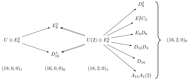
Figure 2. Cusp diagram of $F_{(2,2,0)}$, for $T_{\rm dP}=U\oplus U(2)\oplus E_{8}^{2}$

There are two $0$-cusps which are in bijection with the primitive isotropic lines ${\mathbb{Z}}e\in T_{\rm dP}\mod{\Gamma_{\rm dP}}$, distinguished by the divisibility $\operatorname{div}(e)\in\{1,2\}$ of $e$ in the dual lattice $T_{\rm dP}^{*}$. For a primitive vector in a $2$-elementary lattice one must have $\operatorname{div}(e)\in\{1,2\}$.

The lattices $e^{\perp}/e$ are hyperbolic and $2$-elementary, and here are of the form $U\oplus E_{8}^{2}=(18,0,0)_{1}$ and $U(2)\oplus E_{8}^{2}=(18,2,0)_{1}$ depending on whether $\operatorname{div}(e)=2$ or $1$ respectively. Similarly, the eight $1$-cusps are in bijection with the primitive isotropic planes $\Pi\subset T_{\rm dP}\mod{\Gamma_{\rm dP}}$. For each of them there is a negative-definite lattice $\Pi^{\perp}/\Pi$ which is $2$-elementary but is no longer uniquely determined by the triple $(r,a,\delta)$. The label denotes the root sublattice of $\Pi^{\perp}/\Pi$. Here, $D_{16}$ is a root lattice with determinant $4$ and $D_{16}^{+}$ is its unique even unimodular extension.

The bipartite diagram in Figure 2 depicts all $0$- and $1$-cusps added to compactify $F_{(2,2,0)}$. An arrow indicates that a $0$-cusp lies in the closure of a $1$-cusp. Equivalently, there is, up to the group action, an inclusion ${\mathbb{Z}}e\subset\Pi$ of the corresponding isotropic subspaces.

3.2. Cusp diagram of $F_{(10,10,0)}$

The cusp diagram for ${\overline{F}}_{(10,10,0)}^{\rm BB}$ is well known. It can also be easily found by [AE22, Sec. 5]. We give it in Figure 3, keeping the same notation as above. There are two $0$-cusps distinguished by the divisibility $\operatorname{div}(e)=1$ or $2$.

Figure 3. Cusp diagram of $F_{(10,10,0)}$, for $T_{\rm En}=U\oplus U(2)\oplus E_{8}(2)$

A geometric interpretation of these cusps is as follows. Let ${\mathcal{X}}\to(C,0)$ be a Kulikov model and consider the completed period mapping

$$(C,0)\to{\overline{F}}_{(10,10,0)}^{\rm BB}.$$

Suppose that $\iota_{{\rm En},t}$ on the generic fiber extends to an involution $\iota_{{\rm En},0}$ on the central fiber. If $0\in C$ is sent to the double-circled cusp $(10,10,0)_{1}$ or $(8,8,0)_{0}$ then $\iota_{{\rm En},0}$ is basepoint free. Otherwise, $\iota_{{\rm En},0}$ has a nonempty finite set of fixed points.

Furthermore, the dual complex $\Gamma({\mathcal{X}}_{0})$ is a $2$-sphere and the induced action of $\iota_{{\rm En},0}$ on $\Gamma({\mathcal{X}}_{0})$ in the $(10,10,0)_{1}$ case is an antipodal involution, while in the $(10,8,0)_{1}$ case it is a hemispherical involution, see [AE22, Sec. 8F]. So the quotients of $\Gamma({\mathcal{X}}_{0})$ by the Enriques involution are, respectively, the real projective plane ${\mathbb{R}}{\mathbb{P}}^{2}$ and a disk ${\mathbb{D}}^{2}$. In Type II, $\Gamma({\mathcal{X}}_{0})$ is a segment. In the $(8,8,0)_{0}$ case, the action of $\iota_{{\rm En},0}$ flips the segment, whereas in the $(8,6,0)_{0}$ case it fixes the segment.

3.3. Cusp diagram of $F_{\rm En,2}$

Sterk [Ste91] computed the cusp diagram for ${\overline{F}}_{\rm En,2}^{\rm BB}$. There are five $0$-cusps for which we use Sterk’s numbering $1,2,3,4,5$. There are also $9$ distinct $1$-cusps.

Notation 3.1.

We denote a $1$-cusp by $i_{1}\dots i_{k}$ if its closure contains the $0$-cusps $i_{1},\dotsc,i_{k}$. Here, $1\leq k\leq 5$.

Lemma 3.2.

The morphisms $F_{\rm En,2}\to F_{(2,2,0)}$ and $F_{\rm En,2}\to F_{(10,10,0)}$ extend to the Baily-Borel compactifications, mapping $0$-cusps to $0$-cusps and $1$-cusps to $1$-cusps in the manner shown in Figure 4.

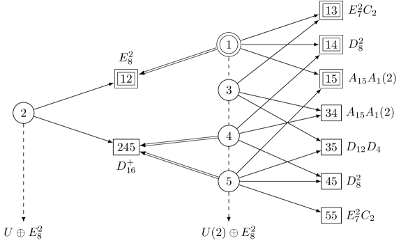
Figure 4. Cusps of ${\overline{F}}_{\rm En,2}^{\rm BB}$ with images in ${\overline{F}}_{(10,10,0)}^{\rm BB}$ and ${\overline{F}}_{(2,2,0)}^{\rm BB}$

The images in ${\overline{F}}_{(2,2,0)}^{\rm BB}$ are shown by labels from Figure 4, and in ${\overline{F}}_{(10,10,0)}^{\rm BB}$ by the corresponding border shapes (oval, double oval, rectangle, double rectangle).

Proof.

The extension property holds by [KK72]. The maps on $0$-cusps are easy to see by looking at the divisibilities of Sterk’s isotropic vectors $e_{1},\dotsc,e_{5}$ considered separately as vectors in the lattices $T_{\rm En}$ and $T_{\rm dP}$. The maps on $1$-cusps are then recovered by considering incidences between $0$- and $1$-cusps and the images of the $1$-cusps in the Baily-Borel compactification ${\overline{F}}_{4}^{\rm BB}\supset{\overline{F}}_{(2,2,0)}^{\rm BB}$ of the moduli space of K3 surfaces of degree $4$, computed at the end of [Ste91]. ∎

3.4. Vinberg’s theory and Coxeter diagrams

We refer to [Vin75, Vin72] for Vinberg’s theory of reflection groups of hyperbolic lattices, saying just enough to fix the notations.

Let $\Lambda$ be a hyperbolic lattice. Let ${\mathcal{C}}$ be the component of the set $\{v\in\Lambda_{\mathbb{R}}\mid v^{2}>0\}$, containing a fixed class $h$ with $h^{2}>0$. Let ${\mathcal{H}}={\mathbb{P}}{\mathcal{C}}$ be the corresponding hyperbolic space. A vector $v\neq 0$ with $v^{2}=0$ in the closure of ${\mathcal{C}}$ defines a point on the sphere at infinity of ${\mathcal{H}}$. Let $\overline{{\mathcal{C}}}$ denote the closure of ${\mathcal{C}}$.

A reflection in a vector $\alpha\in\Lambda$ is the isometry

$$w_{\alpha}(v)=v-\frac{2(\alpha\cdot v)}{\alpha\cdot\alpha}\alpha.$$

A root is a vector $\alpha$ with $\alpha^{2}<0$ such that $w_{\alpha}(\Lambda)=\Lambda$, equivalently such that $2\operatorname{div}(\alpha)\in(\alpha\cdot\alpha){\mathbb{Z}}$. For a group of isometries $\Gamma\subset O(\Lambda)$ we denote by $W(\Gamma)$ its subgroup generated by reflections.

We denote by ${\mathfrak{C}}$ the fundamental chamber for $W(\Gamma)$. Equivalently, one can treat it as the (possibly infinite) polyhedron $P={\mathbb{P}}{\mathfrak{C}}\subset{\mathcal{H}}$. One has

(2) $${\mathfrak{C}}=\left\{v\in{\mathcal{C}}\mid\alpha_{i}\cdot v\geq 0\text{ for simple roots }\alpha_{i}\right\}$$

(3) $$O(\Lambda)=S\ltimes W(\Gamma)\quad\text{for some }S\subset\operatorname{Sym}(P).$$

The fundamental chamber is encoded in a Coxeter diagram. The vertices correspond to the simple roots $\alpha_{i}$ and the edges show the angles between them as follows. Let $g_{ij}=(\alpha_{i}\cdot\alpha_{j})/\sqrt{(\alpha_{i}\cdot\alpha_{i})(\alpha_{j}\cdot\alpha_{j})}$. One connects $i$ and $j$ by

• an $m$-tuple line if $g_{ij}=\cos\frac{\pi}{m+2}$. The hyperplanes $\alpha_{i}^{\perp}$, $\alpha_{j}^{\perp}$ intersect in ${\mathcal{H}}$.

• a thick line if $g_{ij}=1$. $\alpha_{i}^{\perp}$, $\alpha_{j}^{\perp}$ are parallel, meet at an infinite point of ${\mathcal{H}}$.

• a dotted line if $g_{ij}>1$. $\alpha_{i}^{\perp}$, $\alpha_{j}^{\perp}$ do not meet in ${\mathcal{H}}$ or its closure.

The lattices $L_{\rm En}^{\pm}$ and $L_{\rm dP}^{\pm}$ are even $2$-elementary. For such lattices the roots are the $(-2)$-vectors and the $(-4)$-vectors with $\operatorname{div}(\alpha)=2$. We denote the roots with $\alpha^{2}=-2$ by white vertices and those with $\alpha^{2}=-4$ by black vertices.

3.5. Coxeter diagrams for the $0$-cusps of $F_{(2,2,0)}$

The Coxeter diagrams for the lattices $(18,0,0)_{1}=U\oplus E_{8}^{2}$ and $(18,2,0)_{1}=U(2)\oplus E_{8}^{2}$, cf. [AE22], are shown in Figure 5. To describe Kulikov models and KSBA stable models, it is important to keep track of the even and odd nodes on the boundaries of these diagrams. We assign even numbers to the even nodes; in Figure  5 they are shown as double-circled nodes. For typographical reasons, in the diagrams that follow we skip these double circles. The corners are always even.

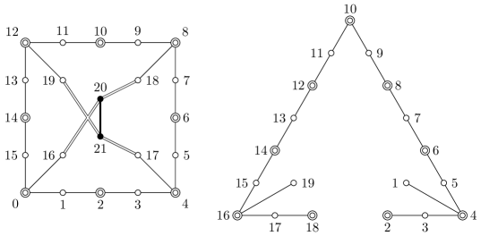
Figure 5. Coxeter diagrams for $(18,2,0)_{1}$ and $(18,0,0)_{1}$

The lattice $U\oplus E_{8}^{2}$ is generated by $19$ roots $\alpha_{1},\dotsc,\alpha_{19}$ with a single relation

(4) $$\begin{aligned} v&=3\alpha_{1}+2\alpha_{2}+4\alpha_{3}+6\alpha_{4}+5\alpha_{5}+4\alpha_{6}+3\alpha_{7}+2\alpha_{8}+\alpha_{9}\\ &=3\alpha_{19}+2\alpha_{18}+4\alpha_{17}+6\alpha_{16}+5\alpha_{15}+4\alpha_{14}+3\alpha_{13}+2\alpha_{12}+\alpha_{11}\end{aligned}$$

The lattice $U(2)\oplus E_{8}^{2}$ is generated by $22$ roots $\alpha_{0},\dotsc,\alpha_{21}$. The relations come from maximal parabolic subdiagrams with more than one connected component. Maximal parabolic subdiagrams correspond to parabolic sublattices with a unique isotropic line; the generator of this line is a linear combination of roots in each connected component, which gives a linear relation. For example, the following relation results from ${\widetilde{E}}_{7}^{2}{\widetilde{C}}_{2}$:

(5) $$\alpha_{16}+\alpha_{20}+\alpha_{18}=\alpha_{1}+2\alpha_{2}+3\alpha_{3}+4\alpha_{4}+3\alpha_{5}+2\alpha_{6}+\alpha_{7}+2\alpha_{17}.$$

3.6. Coxeter diagrams for the $0$-cusps of $F_{(10,10,0)}$

The Coxeter diagrams for the lattices $(10,10,0)_{1}=U(2)\oplus E_{8}(2)$ and $(10,8,0)_{1}=U\oplus E_{8}(2)$ are well-known. They are shown in Figure 6.

Figure 6. Coxeter diagrams for $(10,10,0)_{1}$ and $(10,8,0)_{1}$

3.7. Folding Coxeter diagrams by involutions

Definition 3.3.

Let $\Lambda$ be a lattice with an involution and let $\alpha\in\Lambda$ be a vector. We call the following vector $\alpha_{I}\in\Lambda^{I=1}$ a folded vector:

$$\alpha_{I}=\begin{cases}\alpha&\text{if }I(\alpha)=\alpha\\ \alpha+I(\alpha)&\text{if }I(\alpha)\neq\alpha\\ \end{cases}$$

Lemma 3.4.

Consider the lattice $T_{\rm dP}$ with the involution $I:=-I_{\rm En}=I_{\rm dP}\circ I_{\rm En}=I_{\rm Nik}$, so that $T_{\rm dP}^{I=1}=T_{\rm En}$. Let $\alpha$ be a root of $T_{\rm dP}$ and assume that $\alpha_{I}^{2}<0$. Then $\alpha_{I}$ is a root in $T_{\rm En}$ and one of the following holds:

1. $\alpha^{2}=-2$, $\alpha\in T_{\rm En}$, so $\alpha=\alpha_{I}$ is a root of both $T_{\rm dP}$ and $T_{\rm En}$.

2. $\alpha^{2}=-4$, $\alpha\in T_{\rm En}$, so $\alpha=\alpha_{I}$ is a root of both $T_{\rm dP}$ and $T_{\rm En}$.

3. $\alpha^{2}=-2$, $\alpha\cdot I(\alpha)=0$, $\alpha_{I}^{2}=-4$, and $\alpha_{I}$ is a root of $T_{\rm En}$ but not of $T_{\rm dP}$.

Vice versa, all roots of $T_{\rm En}$ are of these three types.

Proof.

If $\alpha\in T_{\rm En}$, the claim is clear. Now suppose that $\alpha\not\in T_{\rm En}$, so $\alpha_{I}=\alpha+I(\alpha)$. Write $\alpha\in T_{\rm dP}$ in the block form as in Definition 2.3. Then

$$\alpha=(v,u,-u,e,e^{\prime})\quad\text{and}\quad I(\alpha)=(v,u,-u,-e^{\prime},-e)$$

$$I(\alpha)=\alpha-(0,0,0,e+e^{\prime},e+e^{\prime}),\quad$$

$$\alpha\cdot I(\alpha)=\alpha^{2}-(e+e^{\prime})^{2},\quad\alpha_{I}^{2}=2\alpha^{2}+2\alpha\cdot I(\alpha)$$

Since, $\alpha\neq I(\alpha)$, $e+e^{\prime}$ is a nonzero vector in $E_{8}$. Therefore, $\alpha\cdot I(\alpha)>\alpha^{2}$.

For $\alpha^{2}=-2$ this leaves the only possibility $\alpha\cdot I(\alpha)=0$ and $\alpha_{I}^{2}=-4$. Clearly, $\operatorname{div}(\alpha_{I})=2$ in $T_{\rm En}$ so $\alpha_{I}$ is a root of $T_{\rm En}$. But $\operatorname{div}(\alpha_{I})\neq 2$ in $T_{\rm dP}$. Otherwise, $e-e^{\prime}\in 2E_{8}$, which implies that $(e+e^{\prime})^{2}\equiv 0\pmod{4}$, $\alpha\cdot I(\alpha)\geq 2$ and $\alpha_{I}^{2}\geq 0$.

Now let $\alpha$ be a $(-4)$-root in $T_{\rm dP}$. Since the divisibility of $\alpha$ is $2$, one must have $e,e^{\prime}\in 2E_{8}$, so also $e+e^{\prime}\in 2E_{8}$. But then $-(e+e^{\prime})^{2}\geq 8$, $\alpha\cdot I(\alpha)\geq 4$ and $\alpha_{I}^{2}\geq 0$, a contradiction. This completes the forward direction.

The converse follows from [Nam85, 2.13 and 2.15]: up to $\Gamma_{\rm En}=O(T_{\rm En})$ acting on $T_{\rm En}$ there is only one type of $(-2)$-vector and two types of $(-4)$-vectors. ∎

Definition 3.5.

Consider a primitive vector $e\in T_{\rm En}$ with $e^{2}=0$. We get two hyperbolic lattices

$${\overline{T}}_{\rm En}=e^{\perp}(\text{in }T_{\rm En})/e,\quad{\overline{T}}_{\rm dP}=e^{\perp}(\text{in }T_{\rm dP})/e,\quad\textrm{with }{\overline{T}}_{\rm En}\subset{\overline{T}}_{\rm dP}.$$

There are induced involutions ${\overline{I}}_{\rm En}$ and ${\overline{I}}_{\rm dP}$ on these hyperbolic lattices. We denote $J={\overline{I}}_{\rm En}\circ{\overline{I}}_{\rm dP}=-{\overline{I}}_{\rm En}$, which is an involution on ${\overline{T}}_{\rm dP}$, for which the $(+1)$-eigenspace of $J$ in ${\overline{T}}_{\rm dP}$ is ${\overline{T}}_{\rm En}$.

Definition 3.6.

Let $e\in T_{\rm En}$ be primitive isotropic. The stabilizer $\Gamma_{{\rm En},2,e}$ of $e$ in $\Gamma_{\rm En,2}$ fits into an exact sequence

$$0\to U_{e}\to\operatorname{Stab}_{\Gamma_{\rm En,2}}(e)\to\Gamma_{{\rm En},2,e}\to 0$$

where $U_{e}$ is the unipotent subgroup, which acts trivially on $e^{\perp}/e={\overline{T}}_{\rm En}$. We define $\Gamma_{{\rm dP},e}$ and $\Gamma_{{\rm En},e}$ similarly.

Denote by $W(\Gamma_{{\rm dP},e})$ the reflection subgroup of $\Gamma_{{\rm dP},e}$. Its Coxeter diagram $G({\overline{T}}_{{\rm dP}})$ is one of the two Coxeter diagrams in Figure 5. Denote by $W(\Gamma_{{\rm En},2,e})$ the reflection subgroup of $\Gamma_{{\rm En},2,e}$; it is generated by reflections in the roots $\alpha\in T_{\rm En}$ with $\alpha\cdot e=0$.

Definition 3.7.

Let $\Lambda$ be an elliptic, parabolic, or hyperbolic lattice with an involution $J$, and let $G$ be its Coxeter diagram. We define the folded diagram $G^{J}$ to be the diagram with the vectors $\alpha_{J}$ for the roots $\alpha$ in $G$ for which the folded vectors $\alpha_{J}$ happen to be roots of $\Lambda^{J=1}$.

Lemma 3.8.

Let ${\mathfrak{C}}$ be a chamber for the action of $W(\Gamma_{{\rm dP},e})$ on the positive cone ${\mathcal{C}}({\overline{T}}_{\rm dP})$ whose intersection with ${\overline{T}}_{{\rm En}}$ has maximal dimension. Then the cone ${\mathfrak{C}}^{J}:={\mathfrak{C}}\cap{\overline{T}}_{\rm En}\otimes{\mathbb{R}}$ is a fundamental chamber for $W(\Gamma_{{\rm En},2,e})$ and its Coxeter diagram is the folded diagram $G({\overline{T}}_{\rm dP})^{J}$.

Proof.

Let $\alpha$ be one of the simple roots in equation (2), so that $\alpha^{\perp}$ is a wall of ${\mathfrak{C}}$. The intersection of the positive cone ${\mathcal{C}}({\overline{T}}_{\rm En})$ with $\alpha^{\perp}$ is the same as with $\alpha_{J}^{\perp}$. If it is nonempty then $\alpha_{J}^{2}<0$. But then $\alpha_{J}$ is a root in ${\overline{T}}_{\rm En}$ by Lemma 3.4. So the walls of ${\mathfrak{C}}^{J}$ are $\alpha_{J}^{\perp}$ for the folded roots in $G({\overline{T}}_{\rm dP})^{J}$ and ${\mathfrak{C}}^{J}$ is the fundamental chamber for the reflection group with Coxeter diagram $G({\overline{T}}_{\rm dP})^{J}$. ∎

3.8. Coxeter diagrams for the $0$-cusps of $F_{\rm En,2}$ by folding

We now find five involutions of the lattices $U\oplus E_{8}^{2}$ and $U(2)\oplus E_{8}^{2}$ and compute folded diagrams for them. We prove that they are the Coxeter diagrams for the groups $\Gamma_{{\rm En},2,e}$ for some isotropic vectors $e\in T_{\rm En}$. These turn out to be the same as the Coxeter diagrams computed in [Ste91] by Vinberg’s method [Vin75]. We keep Sterk’s numbering for the $0$-cusps. In the order of appearance, they are 2, 1, 3, 4, 5.

Lemma 3.9.

On the Coxeter diagram for the lattice ${\overline{T}}_{\rm dP}=(18,0,0)_{1}$, consider the reflection $J\colon\alpha_{k}\to\alpha_{20-k}$ about the vertical line. Then ${\overline{T}}_{\rm dP}^{J=1}\simeq U\oplus E_{8}(2)$ and the folded diagram is shown in Figure 7.

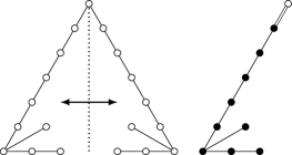
Figure 7. Folded diagram for cusp 2

Proof.

The sublattice ${\overline{T}}_{\rm dP}^{J=1}$ is generated by the vectors $\alpha_{k}+\alpha_{20-k}$, $1\leq k\leq 8$ spanning $E_{8}(2)$ and two vectors spanning an orthogonal $U$: $\alpha_{10}$ along with the vector $v$ in the relation (4). The computation of the folded Coxeter diagram is immediate. ∎

Lemma 3.10.

Consider the following involutions $J$ on the lattice ${\overline{T}}_{\rm dP}=(18,2,0)_{1}$:

1. rotation of the diagram by $180$ degrees.

2. reflection of the diagram about the diagonal, followed by a lattice reflection in the root $\alpha_{20}$.

3. reflection of the diagram about a horizontal line.

4. the composition of $8$ commuting reflections in the roots $\alpha_{1},\alpha_{3},\dotsc,\alpha_{15}$.

The fixed sublattice ${\overline{T}}_{\rm dP}^{J=1}$ is isomorphic to $U(2)\oplus E_{8}(2)$ in case (1) and to $U\oplus E_{8}(2)$ in cases (3,4,5). The folded diagrams are shown in Figure 8.

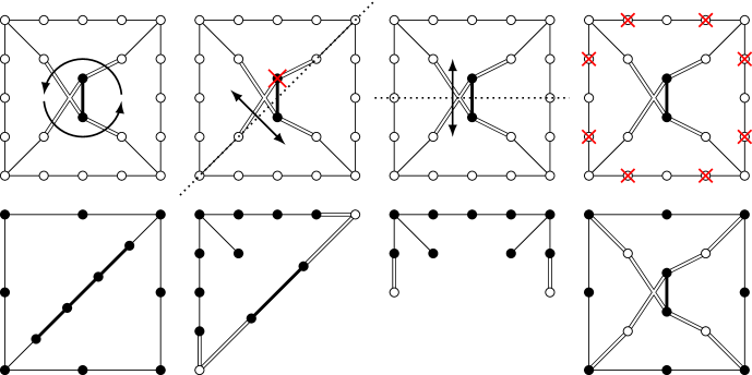
Figure 8. Folded diagrams for cusps 1, 3, 4, 5

Proof.

The computation of the folded Coxeter diagrams is immediate. The fixed sublattices are computed as follows. In all cases the roots generate an index-$2$ sublattice of ${\overline{T}}_{\rm dP}^{J=1}$.

The Coxeter diagram for cusp 1 contains a copy of ${\widetilde{E}}_{8}(2)$, cf. diagram 12 in Figure 10, and so contains a copy of $E_{8}(2)$. Half of the isotropic vector of ${\widetilde{E}}_{8}(2)$ is integral, i.e. lies in ${\overline{T}}_{\rm dP}^{J=1}$. Together with the root disjoint from $E_{8}(2)$, these two elements form an orthogonal copy of $U(2)$, and together they span ${\overline{T}}_{\rm dP}^{J=1}$. This gives ${\overline{T}}_{\rm dP}^{J=1}=U(2)\oplus E_{8}(2)$.

For cusp 3 we observe from diagram 31 in Figure 10 that the Coxeter diagram contains a copy of $({\widetilde{E}}_{7}{\widetilde{A}}_{1})(2)$, i.e. ${\widetilde{E}}_{7}{\widetilde{A}}_{1}$ with the doubled bilinear form. Inside it is a copy of $(E_{7}A_{1})(2)$ which is an index-$2$ sublattice of $E_{8}(2)$. One checks that this $E_{8}(2)$ is indeed a sublattice of ${\overline{T}}_{\rm dP}^{J=1}$. Half of the isotropic vector of ${\widetilde{A}}_{1}(2)$ together with the root disjoint from $(E_{7}A_{1})(2)$ form an orthogonal copy of $U$. The computations for cusps 4 and 5 are similar, starting with the subdiagrams ${\widetilde{D}}_{8}(2)$ and $({\widetilde{A}}_{7}{\widetilde{A}}_{1})(2)$, for cusps 41 and 51. We also made a check with sagemath. ∎

Lemma 3.11.

The involution $J$ on lattice ${\overline{T}}_{\rm dP}$ of Lemmas 3.9, 3.10 can be lifted to an involution ${I}$ on $T_{\rm dP}$ with the fixed sublattice $T_{\rm En}$. Taking $I_{\rm En}=-{I}$ gives $T_{\rm dP}^{I_{\rm En}=-1}=T_{\rm En}$.

Proof.

For the involution of Lemma 3.9 the statement is obvious: we simply define ${I}$ to be the identity on the first summand of $T_{\rm dP}=U(2)\oplus{\overline{T}}_{\rm dP}$. Similarly for cusp (1) in Lemma 3.10 one has $T_{\rm dP}=U\oplus{\overline{T}}_{\rm dP}$ and we extend ${I}$ to $U$ as the identity.

In the cases (3,4,5) we have an exact sequence of abelian groups

$$0\to U\to T_{\rm dP}=U\oplus{\overline{T}}_{\rm dP}\to{\overline{T}}_{\rm dP}\to 0$$

with ${\overline{T}}_{\rm dP}=U(2)\oplus E_{8}^{2}$, ${\overline{T}}_{\rm dP}^{J=1}=U\oplus E_{8}(2)$, and the trivial extension does not work.

Write $U=\langle e,f\rangle$ using the standard basis with $e^{2}=f^{2}=0$, $e\cdot f=1$. A section $s\colon{\overline{T}}_{\rm dP}\to{\mathbb{Z}}e\oplus{\overline{T}}_{\rm dP}\subset U\oplus{\overline{T}}_{\rm dP}$ is the same as an element $a\in{\overline{T}}_{\rm dP}^{*}$, so that $x\mapsto x+a(x)$. The orthogonal complement of ${\overline{T}}_{\rm dP}$ is $\langle e,f-a\rangle\simeq U$ if $a\in{\overline{T}}_{\rm dP}$, and $\langle e,2f-2a\rangle$ if $a\notin{\overline{T}}_{\rm dP}$. One has $(2f-2a)^{2}=4a^{2}$. From this, we see that the last lattice is isomorphic to $U(2)$ if the discriminant form of ${\overline{T}}_{\rm dP}$ satisfies $q_{{\overline{T}}_{\rm dP}}(a)\in{\mathbb{Z}}$, and it is isomorphic to $I_{1,1}(2)=\langle 2\rangle\oplus\langle-2\rangle$ otherwise.

The discriminant form of ${\overline{T}}_{\rm dP}$ is the same as for $U(2)=\langle e^{\prime},f^{\prime}\rangle\subset{\overline{T}}_{\rm dP}$. We choose $a=\frac{1}{2}e^{\prime}$ and define the involution $I$ on $T_{\rm dP}$ to be ${J}$ on $s({\overline{T}}_{\rm dP})$ and the identity on its orthogonal complement $U(2)$. Then

$$T_{\rm dP}^{I=1}\simeq U(2)\oplus{\overline{T}}_{\rm dP}^{J=1}\simeq T_{\rm En}.$$

We complete the proof by Lemma 2.4. ∎

Corollary 3.12.

The above five folded diagrams $G({\overline{T}}_{\rm dP})^{J}$ are precisely the Coxeter diagrams for the reflection groups $W(\Gamma_{{\rm En},2,e})$ for the isotropic vectors $e\in T_{\rm En}\pmod{\Gamma_{\rm En,2}}$.

Proof.

By Lemmas 3.8, 3.9, 3.10, 3.11 the five diagrams we have found are Coxeter diagrams for the reflection groups $W(\Gamma_{{\rm En},2,e})$ for some isotropic vectors $e\in T_{\rm En}$. By [Ste91] the space $F_{\rm En,2}$ has exactly five $0$-cusps, so we have found them all. ∎

Indeed, our Coxeter diagrams, obtained by folding, coincide with the ones found by Sterk in [Ste91] who used the Vinberg algorithm [Vin75] to compute them.

Second proof, without using [Ste91].

By Lemmas 3.8 and 3.11 it is sufficient to find all involutions ${J}$ on hyperbolic lattices ${\overline{T}}_{\rm dP}=U\oplus E_{8}^{2}$ and ${\overline{T}}_{\rm dP}=U(2)\oplus E_{8}^{2}$ for which the sublattice ${\overline{T}}_{\rm dP}^{J=1}$ is isomorphic to $U(2)\oplus E_{8}(2)$ or $U\oplus E_{8}(2)$ and such that the folded root vectors define a chamber ${\mathfrak{C}}^{J}$ lying inside a chamber ${\mathfrak{C}}$ for the Coxeter diagram $G({\overline{T}}_{\rm dP})$. Any such involution is a product of an involution of the diagram $G({\overline{T}}_{\rm dP})$, which may be the identity, composed with a commuting involution in the Weyl group. It is well known that an involution in a Coxeter group is a composition of commuting reflections.

Under the condition $\operatorname{rk}\,{\overline{T}}_{\rm dP}^{J=1}=10$, this reduces the check to the following possibilities, in addition to the ones in Lemma 3.9 and cases (1,4) of Lemma 3.10:

1. a composition of reflections in $8$ orthogonal roots of $G(U\oplus E_{8}^{2})$.

2. the diagonal involution of $G(U(2)\oplus E_{8}^{2})$ composed with a single reflection in $\alpha_{0}$, $\alpha_{8}$, $\alpha_{16}$, $\alpha_{18}$, $\alpha_{20}$ or $\alpha_{21}$.

3. a composition of reflections in $8$ orthogonal roots of $G(U(2)\oplus E_{8}^{2})$.

The first case does not occur. We confirmed with sagemath that ${\overline{T}}_{\rm dP}^{J=1}$ is never isomorphic to $U(2)\oplus E_{8}(2)$, and that it is isomorphic to $U\oplus E_{8}(2)$ only in the second case for $\alpha_{20}$, and in the last case for $\{\alpha_{1},\alpha_{3},\dotsc,\alpha_{15}\}$. ∎

3.9. $1$-cusps of $F_{\rm En,2}$ by folding

Lemma 3.13.

The $1$-cusps of $F_{\rm En,2}$ correspond to the maximal parabolic subdiagrams of the Coxeter diagrams of $U\oplus E_{8}^{2}$ and $U(2)\oplus E_{8}^{2}$ which are symmetric with respect to one of the five involutions of Lemma 3.10. For cusps 3 and 5 this means that the subdiagram has to contain the roots $\alpha_{20}$, resp. $\alpha_{1},\alpha_{3},\dots,\alpha_{15}$ in which the reflections are made.

Indeed, both correspond to the isotropic planes contained in the sublattice of $T$ fixed by the involution. We list these $1$-cusps in Figures 9 and 10. They agree with Sterk’s computations in [Ste91], and the entire cusp diagram agrees with Figure 4.

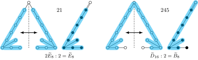
Figure 9. $1$-cusps of $F_{\rm En,2}$ passing through $0$-cusp 2

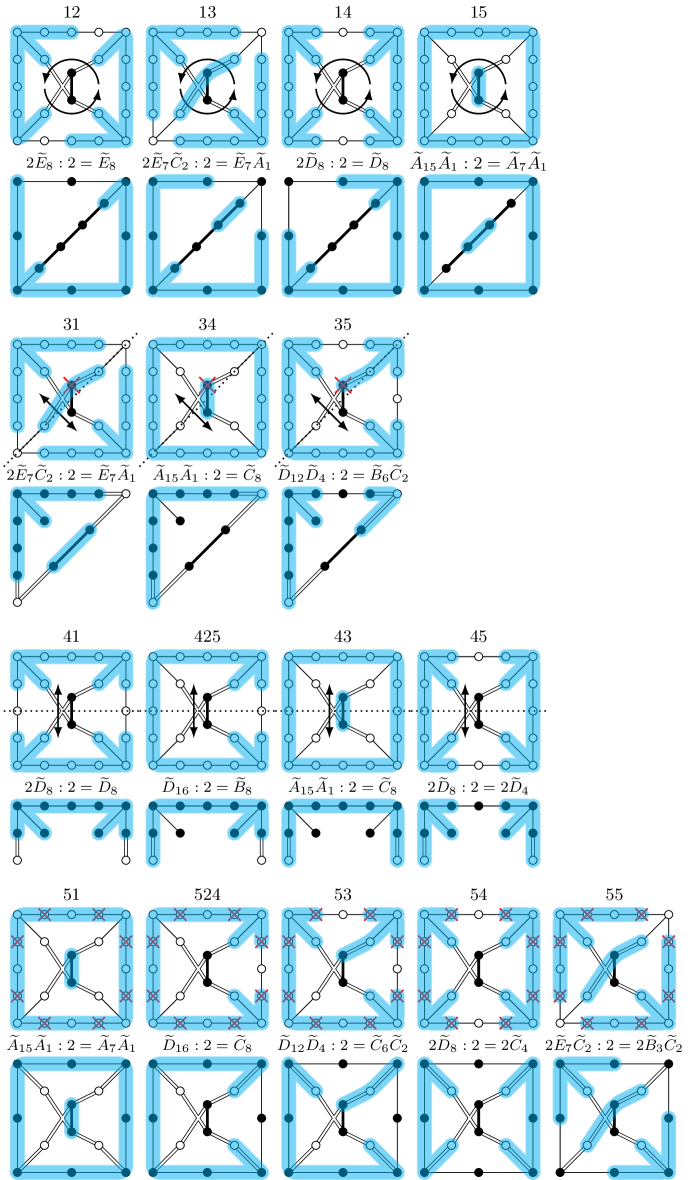
Figure 10. $1$-cusps of $F_{\rm En,2}$ passing through $0$-cusps 1, 3, 4, 5

Figures 9, 10 contain the information of all cusp incidences of ${\overline{F}}_{\rm En,2}^{\rm BB}$. The figures are read as follows: the first numeral indicates one of the five folding symmetries $1,2,3,4,5$ of the relevant hyperbolic lattice ${\overline{T}}_{\rm dP}$, and this symmetry is also depicted on the Coxeter diagram for ${\overline{T}}_{\rm dP}$, with an $\times$ indicating that we reflect in the corresponding root. These correspond to the five $0$-cusps added to $F_{\rm En,2}$.

In blue is highlighted a maximal parabolic subdiagram invariant under the given folding symmetry. Necessarily, all $\times$-ed vertices are contained in this diagram, since only these diagrams can be invariant under the corresponding composition of root reflections. Such blue diagrams are in bijection with the $1$-cusps incident upon the corresponding $0$-cusp. The collection of all numerals, including the first label, indicate the corresponding $1$-cusp, see Notation 3.1.

Finally, adjacent to each maximal parabolic diagram for ${\overline{T}}_{\rm dP}$ is the corresponding maximal parabolic subdiagram of the folded lattice ${\overline{T}}_{\rm En}$.

Remark 3.14.

The $1$-cusps $E_{8}D_{8}$ and $D_{16}$ of $F_{(2,2,0)}$ do not appear as images of $1$-cusps of $F_{\rm En,2}$. The reason is now clear: these are exactly the two of the eight $1$-cusps of $F_{(2,2,0)}$ for which the parabolic subdiagrams, that can be found e.g. in [AE22], are not symmetric with respect to any of the four involutions in Lemma 3.10.

Remark 3.15.

The idea that folded diagrams may be relevant to compactifying $F_{\rm En,2}$ implicitly appears in [Ste91], e.g. there is a folded $A_{15}$ diagram in Fig. 16. We found that once the K3 case understood, the folding, when applied to the correct space—which is $F_{(2,2,0)}$ and not $F_{4}$—completely solves the Enriques case. Note that the moduli space $F_{4}$ of quartic K3 surfaces has a unique $0$-cusp with a non-reflective hyperbolic lattice, but the moduli space $F_{(2,2,0)}$ of hyperelliptic K3 surfaces of degree $4$ has two $0$-cusps with reflective hyperbolic lattices; see Figure 5.

4. Dlt models via integral-affine structures on the disk and ${\mathbb{R}}{\mathbb{P}}^{2}$

4.1. General theory

The general theory of integral affine spheres, $\operatorname{IAS^{2}}$ for short, in the form that we need it here is detailed in [Eng18, EF21, ABE22, AET23, AE22]. We refer the reader to the above papers for the necessary background, and give a broad summary now.

A Kulikov model is a $K$-trivial semistable model ${\mathcal{X}}\to(C,0)$ of a degeneration of K3 surfaces over a pointed curve [Kul77], [PP81]. For Type III degenerations, the dual complex $\Gamma({\mathcal{X}}_{0})$ of the central fiber is the $2$-sphere $S^{2}$, and for Type II degenerations $\Gamma({\mathcal{X}}_{0})$ is a segment. By [GHK15a, Rem. 1.1v1], [Eng18, Prop. 3.10] there is a natural integral-affine structure on $\Gamma({\mathcal{X}}_{0})$, with singularities. The correct notion of singularities is detailed in [ABE22, Sec. 5].

Fixing one Kulikov model ${\mathcal{X}}\to(C,0)$, we get Kulikov models for all other degenerations with the same Picard-Lefschetz transform, of the same combinatorial type [FS86, Lem. 5.6], [AE23, Def. 7.14] by deforming the gluings and moduli of components. We can extract the KSBA stable limit of a degeneration $({\mathcal{X}}^{*},\epsilon{\mathcal{R}}^{*})$ of K3 pairs, if we can describe the integral-affine polarization $R_{\rm IA}\subset\Gamma({\mathcal{X}}_{0})$, a certain weighted balanced graph [ABE22, Def. 5.17]. This weighted graph encodes the line bundle ${\mathcal{O}}_{{\mathcal{X}}_{0}}({\mathcal{R}}_{0})$ on a divisor model $({\mathcal{X}},{\mathcal{R}})$: a Kulikov model which admits a nef extension of ${\mathcal{R}}_{t}$, $t\in C\setminus 0$, containing no singular strata of ${\mathcal{X}}_{0}$ [AET23, Thm. 3.12], [Laz16, Thm. 2.11].

By [AEH21, Thm. 3.24], our chosen divisor $R$, as the fixed locus of an automorphism $\iota_{\rm dP}$ on a general Enriques K3 surface, is recognizable, see [AE23, Def. 6.2]. By the main theorem on recognizable divisors [AE23, Thm. 1], there is a unique semifan ${\mathfrak{F}}_{R}$ whose corresponding semitoroidal compactification [Loo03], [AE23, Sec. 5C] normalizes the KSBA compactification of $F_{\rm En,2}$. By [AE23, Thm. 8.11(5)], $(\Gamma({\mathcal{X}}_{0}),R_{\rm IA})$ can be chosen to be the same for all degenerations with fixed Picard-Lefschetz transform.

In turn, the combinatorial data of $(\Gamma({\mathcal{X}}_{0}),R_{\rm IA})$ determines the combinatorial type of the KSBA stable limit of the degeneration $(\overline{{\mathcal{X}}}_{0},\epsilon\overline{{\mathcal{R}}}_{0})$ by [AE23, Cor. 8.13]. Then [AE23, Thm. 9.3] gives an algorithm to determine ${\mathfrak{F}}_{R}$: Its cones are given by collections of Picard-Lefschetz transformations for which $(\Gamma({\mathcal{X}}_{0}),R_{\rm IA})$ determines a KSBA-stable pair of a fixed combinatorial type. This is the natural notion of combinatorial constancy of such pairs.

The possible Picard-Lefschetz transformations of Kulikov degenerations in ${\overline{F}}_{\rm En,2}$ are encoded by a vector $\lambda\in{\mathfrak{C}}^{J}$ called the monodromy invariant. It is valued in the fundamental chamber ${\mathfrak{C}}^{J}$ for one of the five folded diagrams $G^{J}=G({\overline{T}}_{{\rm dP}})^{J}$ of Figures 7, 8 as in Lemma 3.8 because $\lambda$ must be invariant under the involution $J$ on ${\overline{T}}_{\rm dP}$. An algorithm (albeit a complicated one), is provided in [AE22, Thm. 8.3] to build $(\Gamma({\mathcal{X}}_{0}),R_{\rm IA})$ for all monodromy invariants $\lambda\in{\mathfrak{C}}$ in the fundamental chamber for the Weyl group action, for either hyperbolic lattice ${\overline{T}}_{\rm dP}=(18,2,0)_{1}$ or ${\overline{T}}_{\rm dP}=(18,0,0)_{1}$ corresponding to a $0$-cusp of $F_{(2,2,0)}$.

Restricting $\operatorname{IAS^{2}}$ for $F_{(2,2,0)}$ to the involution-invariant sublattice ${\overline{T}}={\overline{T}}_{{\rm dP}}^{J=1}$ exhibits a polarized $\operatorname{IAS^{2}}$ for any Type III degeneration in ${\overline{F}}_{\rm En,2}$. Then, one can hope (and it is indeed the case, as shown below), that on these subloci, the corresponding divisor models $({\mathcal{X}},{\mathcal{R}})$ admit a second involution identified with the limit of the Enriques involution. Thus, these polarized $\operatorname{IAS^{2}}$ will provide a method to compute the Kulikov and KSBA-stable models of all degenerations of both the Enriques surfaces and their corresponding double covers, the Enriques K3 surfaces.

Definition 4.1.

Let $\lambda\in{\mathfrak{C}}$, for the one of the two $0$-cusps of $F_{(2,2,0)}$. We define

$$\ell:=(\ell_{i})_{i\in G}=(\lambda\cdot\alpha_{i})_{i\in G}$$

where $\alpha_{i}$ are the roots of either diagram in Figure 5. Thus, $\ell\in({\mathbb{Z}}_{\geq 0})^{22}$ for the cusp $(18,2,0)_{1}$ and $\ell\in({\mathbb{Z}}_{\geq 0})^{19}$ for the cusp $(18,0,0)_{1}$.

4.2. $\operatorname{IAS^{2}}$ for $F_{(2,2,0)}$

We now identify the polarized $\operatorname{IAS^{2}}$ for degenerations in $F_{(2,2,0)}$ following the instructions of [AE22, Thms. 7.4, 8.3]. We treat each of the two $0$-cusps individually.

Cusp $(18,2,0)_{1}$: We are to first take a K3 surface ${\widehat{X}}$ in the mirror moduli space for this $0$-cusp—these are $U(2)\oplus E_{8}^{\oplus 2}$-polarized K3 surfaces. Then we are to consider the anticanonical pair quotient

$$({\widehat{Y}},{\widehat{D}}):={\widehat{X}}/\,\widehat{\iota}_{\rm dP}$$

by the mirror involution and, for each ${\widehat{L}}$ in the nef cone of ${\widehat{Y}}$, we must build a Symington polytope $P(\ell)$ for the line bundle ${\widehat{L}}\to({\widehat{Y}},{\widehat{D}})$ corresponding to $\ell$, see [Sym03], [AE22, Construction 6.16]. We build a sphere $B(\ell)=P(\ell)\cup P(\ell)^{\rm opp}$ by identifying two copies of this integral-affine disk along their common boundary, to form the equator of the sphere. Then $B(\ell)=\Gamma({\mathcal{X}}_{0})$ for a monodromy-invariant $\lambda\leftrightarrow\ell\leftrightarrow{\widehat{L}}$ and the integral-affine polarization $R_{\rm IA}$ corresponding to the flat limit ${\mathcal{R}}_{0}\subset{\mathcal{X}}_{0}$ is the equator of the sphere, with weights alternating $2$ and $1$.

The anticanonical pair $({\widehat{Y}},{\widehat{D}})$ is a rational elliptic surface with an anticanonical cycle of $16$ curves, of alternating self-intersections $-1$ and $-4$, which result from blowing up the corners of an $I_{8}$ Kodaira fiber. This pair admits a toric model

$$({\widehat{Y}},{\widehat{D}})\to(\overline{{\widehat{Y}}},\overline{{\widehat{D}}})$$

whose fan is depicted on the left-hand side of Figure 17. The rays going to the four corners correspond to components of the toric model receiving an internal blow-up, i.e. a blow-up at a smooth point of the anticanonical boundary.

A moment polytope ${\overline{P}}(\ell)$ for the line bundle $\overline{{\widehat{L}}}\to(\overline{{\widehat{Y}}},\overline{{\widehat{D}}})$ is depicted on the left of Figure 12 and a Symington polytope $P(\ell)$ for the line bundle ${\widehat{L}}\to({\widehat{Y}},{\widehat{D}})$ corresponding to $\ell$ is depicted on the right of Figure 12. The right hand-side also serves as a visualization of each hemisphere of the integral-affine sphere $B(\ell)=\Gamma({\mathcal{X}}_{0})$, with the equator in blue and integral-affine singularities in red. The quantities $\ell_{20}$ and $\ell_{21}$ are, respectively, twice the lattice length between the singularities introduced by Symington surgeries on opposite sides of the figure.

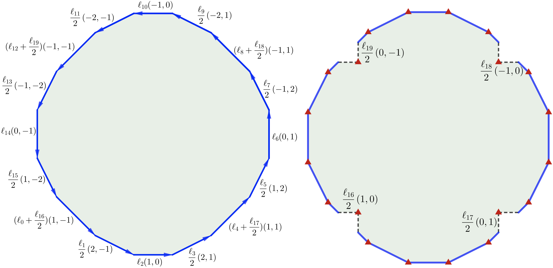
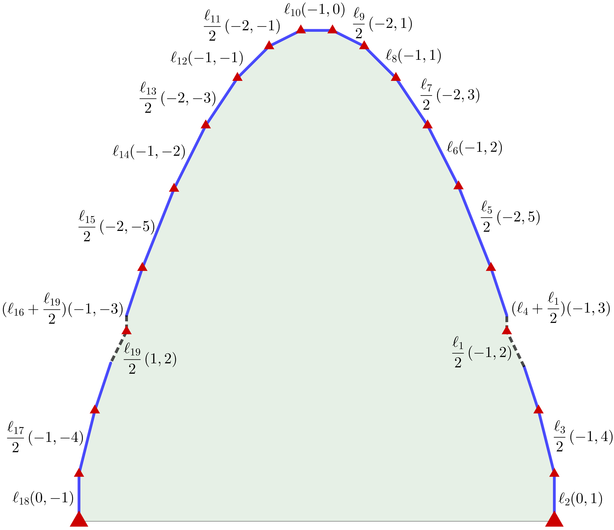
Figure 11. Moment and Symington polytopes for cusp $(18,2,0)_{1}$

Figure 12. Symington polytope for cusp $(18,0,0)_{1}$

Cusp $(18,0,0)_{1}$: The procedure for constructing polarized $\operatorname{IAS^{2}}$ at this cusp is essentially the same as the above, instead taking the mirror moduli space to be $U\oplus E_{8}^{\oplus 2}$-polarized. The fan of a toric model of the mirror is provided by the right hand side of Figure 17. The integral-affine structures are similar to those depicted in [ABE22, Fig. 4], with an important difference: The cusp $(18,0,0)_{1}$ corresponds to a non-simple mirror of $F_{(2,2,0)}$. This means that the integral-affine polarization $R_{\rm IA}\subset B(\ell)$ has no support on the bottom edge of the Symington polytope $P$, and ${\mathcal{R}}_{0}$ is empty on the corresponding components of ${\mathcal{X}}_{0}$. See the discussion of a “B-move” in [AE22, Sec. 8D] for further details.

The $\operatorname{IAS^{2}}$ we need is the result of taking the $\operatorname{IAS^{2}}$ of [ABE22, Fig. 4], splitting the $I_{2}$ singularity at the bottom into two $I_{1}$ singularities traveling in opposite directions, and colliding each one with a corner. This produces singularities in the bottom left and right corners of charge $2$, depicted with a larger red triangle, see Figure 12.

Remark 4.2.

Note that in both cases, certain coordinates of $\ell$ must be divisible by $2$ to build the polarized $\operatorname{IAS^{2}}$. This does not present an issue, since we only need divisor models for all sufficiently divisible $\lambda$.

Remark 4.3.

For the cusp $(18,0,0)_{1}$, the polygon ${\overline{P}}(\ell)$ in Figure 12 can be closed by a horizontal base exactly because of relation (4). The same holds for cusp $(18,2,0)_{1}$ with relation (5) and other similar relations.

To summarize, by [AE22, Thm. 8.3], we have:

Theorem 4.4.

Let $(B(\ell),\,R_{\rm IA})$ be the polarized $\operatorname{IAS^{2}}$ built above, from $\ell\in({\mathbb{Z}}_{\geq 0})^{22}$ or $({\mathbb{Z}}_{\geq 0})^{19}$. Then, upon triangulation into lattice simplices,

$$(B(\ell),R_{\rm IA})=(\Gamma({\mathcal{X}}_{0}),\Gamma({\mathcal{R}}_{0}))$$

is the dual complex of the central fiber $({\mathcal{X}}_{0},{\mathcal{R}}_{0})$ of a divisor model $({\mathcal{X}},{\mathcal{R}})\to(C,0)$, whose monodromy invariant $\lambda\in{\mathfrak{C}}$ satisfies $\ell=(\lambda\cdot\alpha_{i})_{i\in G}$.

4.3. ${\rm IA}{\mathbb{D}}^{2}$ and ${\rm IA}{\mathbb{R}}{\mathbb{P}}^{2}$ for $F_{\rm En,2}$

Now suppose that $({\mathcal{X}},{\mathcal{R}})\to(C,0)$ is a Type III divisor model as in Theorem 4.4, whose period map $C^{*}\to F_{(2,2,0)}$ factors through $F_{\rm En,2}$. Then, the general fiber ${\mathcal{X}}_{t}$ is an Enriques K3 surface with degree $4$ polarization, and $({\mathcal{X}},{\mathcal{R}})\to(C,0)$ is a divisor model for the degeneration. The quotient

$${\mathcal{X}}^{*}/\iota_{{\rm En}}^{*}={\mathcal{Z}}^{*}\to C^{*}$$

of the general fiber by the Enriques involution is a degenerating family of Enriques surfaces. The monodromy invariant $\lambda\in{\mathfrak{C}}^{J}$ then necessarily lies in the fundamental chamber for one of the five $0$-cusps of ${\overline{F}}_{\rm En,2}$. Equivalently, $\ell$ must be invariant under one of the five folding symmetries.

Proposition 4.5.

Let $\lambda\in{\mathfrak{C}}^{J}$, $\ell=(\lambda\cdot\alpha_{i})_{i\in G}$. The folding symmetry $J$ on ${\overline{T}}_{\rm dP}$ induces an isomorphism $\iota_{{\rm En},{\rm IA}}$ of the polarized $\operatorname{IAS^{2}}$ $(B(\ell),\,R_{\rm IA})$ of Theorem 4.4. The dual complexes $\Gamma({\mathcal{X}}_{0},{\mathcal{R}}_{0})$ of divisor models for Enriques K3 surface degenerations in $F_{\rm En,2}$ are exactly those admitting the additional symmetry $\iota_{{\rm En},{\rm IA}}$ (appropriately interpreted for $\times$-ed nodes in cusps 3, 5).

Proof.

For each $0$-cusp, we directly inspect the $\operatorname{IAS^{2}}$ for the parameters $\ell$ corresponding to $\lambda\in{\mathfrak{C}}^{J}$ and see that there is an additional symmetry of $B(\ell)$.

Cusp 2: We have $\lambda\in{\mathfrak{C}}^{J}$ if and only if $\ell_{i}=\ell_{20-i}$ for all $i=1,\dots,9$. The $\operatorname{IAS^{2}}$ in Figure 12 then has a visible symmetry, which is to act on the both the hemisphere $P$, and its opposite hemisphere $P^{\rm opp}$, by a flip across the vertical line bisecting the bottom and top edges.

Cusp 1: We have $\lambda\in{\mathfrak{C}}^{J}$ if and only if $\ell_{i}=\ell_{8+i}$ for all $i=0,\dots,7$, $\ell_{16}=\ell_{18}$ and $\ell_{17}=\ell_{19}$. Then the corresponding involution $\iota_{{\rm En},{\rm IA}}$ of the $\operatorname{IAS^{2}}$ is to rotate each hemisphere, shown in Figure 12, by $180$ degrees, and then flip the two hemispheres $P$ and $P^{\rm opp}$.

Cusp 3: We have $\lambda\in{\mathfrak{C}}^{J}$ if and only if $\ell_{i}=\ell_{16-i}$ for all $i=1,\dots,7$, $\ell_{17}=\ell_{19}$, and $\ell_{20}=0$. This is because the folding symmetry also reflects in the root $\alpha_{20}$. So if $w_{\alpha_{20}}(\lambda)=\lambda$, then $\ell_{20}=\lambda\cdot\alpha_{20}=0$.

Recall that $\ell_{20}$ is the lattice distance between the singularities introduced by the Symington surgeries resting on the edges parallel to $(1,-1)$ and $(-1,1)$, on the right-hand side of Figure 12. We construct $B(\ell)$ in such a way that the two singularities introduced by these Symington surgeries coincide. The involution $\iota_{{\rm En},{\rm IA}}$ of the $\operatorname{IAS^{2}}$ acts by flipping each hemisphere $P$, $P^{\rm opp}$ diagonally.

Cusp 4: Similar to Cusp 2, we have $\lambda\in{\mathfrak{C}}^{J}$ if and only if each hemisphere of $B(\ell)$ is symmetric with respect to flipping along a horizontal line bisecting the edges $\ell_{6}(0,1)$ and $\ell_{14}(0,-1)$.

Cusp 5: We have $\lambda\in{\mathfrak{C}}^{J}$ if and only if $\ell_{2i+1}=0$ for $i=0,\dots,7$. We declare that $\iota_{{\rm En},{\rm IA}}$ act in the same manner as the extension of $\iota_{{\rm dP}}$ to ${\mathcal{X}}_{0}$: It flips the two hemispheres $P$ and $P^{\rm opp}$. The eight $\times$-ed nodes correspond to eight collisions of pairs of $I_{1}$ singularities along the equator.

By [AE22, Prop. 6.17], the mirror K3 surface ${\widehat{X}}$ admits a symplectic form $\omega$ and Lagrangian torus fibration

$$\mu\colon({\widehat{X}},\omega)\to B(\ell),$$

for generic $\ell\in{\mathfrak{C}}^{J}$. Note that while some of the $24$ $I_{1}$-singularities collide on $B(\ell)$ for Cusps 3 and 5, we only ever get, for generic $\ell$, a collision of two $I_{1}$-singularities with parallel $\operatorname{SL}_{2}({\mathbb{Z}})$-monodromies. So the fibration $\mu$ still exists, but has $I_{2}$ fibers over these collisions.

The involution $\iota_{{\rm En},{\rm IA}}$ acting on $B(\ell)$ induces an involution of the Lagrangian torus fibration $({\widehat{X}},\mu)$ and in turn on ${\rm Pic}({\widehat{X}})\simeq{\overline{T}}_{\rm dP}=(18,2,0)_{1}$ or $(18,0,0)_{1}$ which is generated by classes of visible curves, cf. [AE22, Sec. 6G]. In the current setting, the visible curves (which correspond to the roots $\alpha_{i}$) are all of the following simple form: A path connecting two $I_{1}$-singularities with parallel $\operatorname{SL}_{2}({\mathbb{Z}})$-monodromies. For Cusps 1, 2, 4, the involution $\iota_{{\rm En},{\rm IA}}$ acts on the classes of visible curves by the Enriques involution on ${\overline{T}}_{\rm dP}$ and thus, by the Mirror/Monodromy Theorem [EF21, Prop. 3.14], [AE22, Thms. 6.19, 7.6], $B(\ell)$ is the dual complex of a degeneration with a monodromy invariant in ${\overline{T}}_{\rm dP}^{J=1}$.

Some additional care must be taken for Cusps 3 and 5, where $B(\ell)$ is a limit of $\operatorname{IAS^{2}}$ with $24$ distinct $I_{1}$-singularities. For each $\times$-ed node, the involution $J$ acts on ${\overline{T}}_{\rm dP}$ by reflecting along $\alpha_{i}$ and so the class $[\omega]$ of the symplectic form should satisfy $[\omega]\cdot\alpha_{i}=0$. Equivalently, there should be a nodal slide, see [AE22, Sec. 6E], which collides the two $I_{1}$ singularities of the visible curve corresponding to $\alpha_{i}$ into an $I_{2}$ singularity. This is indeed the case for the $\operatorname{IAS^{2}}$ described above. To summarize, invariance under reflection of an $\times$-ed node $\alpha_{i}$ corresponds, on the $\operatorname{IAS^{2}}$, to colliding the two $I_{1}$ singularities bounding the corresponding visible curve.

We conclude that an $\iota_{{\rm En},{\rm IA}}$-invariant polarized $\operatorname{IAS^{2}}$, which has a coalescence to an $I_{2}$-singularity for each $\times$-ed node, is the dual complex of a divisor model $({\mathcal{X}},{\mathcal{R}})\to(C,0)$ for degree $4$ Enriques K3 surfaces whose monodromy invariant $\lambda\in{\mathfrak{C}}^{J}$ is generic. The passage from the result for generic $\lambda\in{\mathfrak{C}}^{J}$ to all $\lambda\in{\mathfrak{C}}^{J}$ is a standard trick involving a limit procedure on the corresponding $\operatorname{IAS^{2}}$, examining $B(\ell)$ as some $\ell_{i}\to 0$, see [AET23, Thm. 6.29], [AE22, Sec. 6G]. ∎

Theorem 4.6.

For all $\lambda\in{\mathfrak{C}}^{J}$, the general divisor model $({\mathcal{X}},{\mathcal{R}})\to(C,0)$ with monodromy invariant $\lambda$ admits a second involution $\iota_{\rm En}\colon{\mathcal{X}}\to{\mathcal{X}}$ extending the Enriques involution on the general fiber, and satisfying $\iota_{\rm En}({\mathcal{R}})={\mathcal{R}}$.

Proof.

The proof is essentially the same as [AE22, Thm. 8.3]. The key point is that the Kulikov models ${\mathcal{X}}_{0}$ which arise as limits of Enriques K3s are those whose period point $\varphi_{{\mathcal{X}}_{0}}\in{\rm Hom}(\lambda^{\perp}({\overline{T}}_{\rm dP}),{\mathbb{C}}^{*})$ is anti-invariant under $\iota_{{\rm En},{\rm IA}}$—we require anti-invariance because $\iota_{{\rm En},{\rm IA}}$ acts in an orientation reversing manner on $\Gamma({\mathcal{X}}_{0})$.

The anti-invariant periods are those $\varphi_{X_{0}}$ for which $(S_{\rm dP})^{\perp}_{S_{\rm En}}=E_{8}(2)\subset\ker(\varphi_{{\mathcal{X}}_{0}})$, and the smoothings keeping these classes Cartier are exactly those admitting an $S_{\rm En}$-polarization (and hence admitting an Enriques involution). Finally, the Kulikov surfaces ${\mathcal{X}}_{0}$ with an anti-invariant period are also identified with those admitting an additional involution $\iota_{{\rm En},0}$ because the ${\mathbb{C}}^{*}$-moduli of components and their gluings are made invariantly with respect to the action of $\iota_{{\rm En},{\rm IA}}$ on the gluing complex [AE23, Def. 5.10]. Furthermore, the deformations keeping the involution $\iota_{{\rm En},0}$ are then identified with those keeping the $S_{\rm En}$-polarization.

Since the divisor model is generic, [AE22, Thm. 8.3] implies that ${\mathcal{R}}\subset{\mathcal{X}}$ is the divisorial component of the fixed locus of an involution $\iota_{{\rm dP}}$ on the threefold ${\mathcal{X}}$ extending the del Pezzo involution on the general fiber. Then $\iota_{\rm dP}$ and $\iota_{{\rm En}}$ commute on the general fiber and hence commute on all of ${\mathcal{X}}$. So $\iota_{\rm En}$ preserves ${\mathcal{R}}$. ∎

More generally, every degeneration of Enriques surfaces admits a divisor model $({\mathcal{X}},{\mathcal{R}})\to(C,0)$ for which $\iota_{{\rm En}}$ defines a birational involution, and for which the union of the fixed locus and the locus of indeterminacy contains ${\mathcal{R}}$.

Definition 4.7.

Let ${\mathcal{X}}\to(C,0)$, $({\mathcal{X}},{\mathcal{R}})\to(C,0)$ be a Kulikov, resp. divisor, model of Enriques K3 surfaces for which $\iota_{{\rm En}}$ defines a regular involution on ${\mathcal{X}}$, resp. preserving ${\mathcal{R}}$. We define the dlt model, resp. the half-divisor model, to be the quotient by the Enriques involution:

$${\mathcal{Z}}:={\mathcal{X}}/\iota_{{\rm En}},\quad\textrm{resp.~{}}\quad({\mathcal{Z}},{\mathcal{R}}_{\mathcal{Z}}):=({\mathcal{X}},{\mathcal{R}})/\iota_{{\rm En}}.$$

Proposition 4.8.

Let $({\mathcal{Z}},{\mathcal{R}}_{\mathcal{Z}})\to(C,0)$ be a half-divisor model for $F_{\rm En,2}$ for the divisor models constructed in Proposition 4.5. Then, the fibers of ${\mathcal{Z}}$ have slc singularities, $K_{\mathcal{Z}}+\epsilon{\mathcal{R}}_{\mathcal{Z}}$ is relatively big and nef over $C$, and ${\mathcal{R}}_{\mathcal{Z}}$ contains no log canonical centers. In Type III, for cusp number

1. we have $\Gamma({\mathcal{Z}}_{0})={\mathbb{R}}{\mathbb{P}}^{2}$. Each component $V_{i}\subset{\mathcal{Z}}_{0}$ is isomorphic, up to normalization, with either of the two connected components of its inverse image in ${\mathcal{X}}_{0}$.

2. we have $\Gamma({\mathcal{Z}}_{0})={\mathbb{D}}^{2}$. If the component $V_{i}\subset{\mathcal{Z}}_{0}$ is covered by two irreducible components of ${\mathcal{X}}_{0}$ then up to normalization, $V_{i}$ is isomorphic to either of these components. If $V_{i}\subset{\mathcal{Z}}_{0}$ is covered by one irreducible component of ${\widetilde{V}}_{i}\subset{\mathcal{X}}_{0}$ then $\iota_{{\rm En},0}$ acts on ${\widetilde{V}}_{i}$ with exactly four fixed points, two pairs of points on appropriately chosen double curves ${\widetilde{D}}_{ij}$ and ${\widetilde{D}}_{ik}\subset{\widetilde{V}}_{i}$.

In Type II, $\Gamma({\mathcal{Z}}_{0})$ is a segment. For cases in Fig. 4 with a double rectangle, $\iota_{{\rm En},0}$ acts by flipping $\Gamma({\mathcal{X}}_{0})$ and fixing no points of ${\mathcal{X}}_{0}$. Assuming that ${\mathcal{X}}_{0}$ contains a double curve $E$ preserved by $\iota_{{\rm En},0}$, the action of the involution on $E$ is a nontrivial $2$-torsion translation. For cases in Fig. 4 with a single rectangle, $\iota_{{\rm En},0}$ preserves every component of ${\mathcal{X}}_{0}$. On any double curve, the action is by an elliptic involution fixing exactly four points. There are no other fixed points on ${\mathcal{X}}_{0}$.

Proof.

In Type III, the homeomorphism type of $\Gamma({\mathcal{Z}}_{0})$ follows directly from the description of the action of $\iota_{{\rm En},{\rm IA}}$ in Proposition 4.5. In Type II, we can construct divisor models $({\mathcal{X}},{\mathcal{R}})\to(C,0)$ by taking limits of $B(\ell)$ as it collapses to a segment, or equivalently as $\lambda$ approaches a rational isotropic ray at the boundary of $\overline{{\mathcal{C}}}$.

The resulting central fiber ${\mathcal{X}}_{0}$ is a chain of surfaces and by arguments similar to Theorem 4.6, a general degeneration $({\mathcal{X}},{\mathcal{R}})$ to the given Type II boundary divisor admits an additional involution $\iota_{\rm En}$ which acts on $\Gamma({\mathcal{X}}_{0})$ by the limit of the action of $\iota_{{\rm En},{\rm IA}}$ on the segment $B(\ell)$. This gives the claimed action on $\Gamma({\mathcal{X}}_{0})$, by direct examination of the limiting dual segment $B(\ell)$ for all entries of Figures 9, 10.

If $\iota_{{\rm En},0}$ permutes two irreducible components, it is clear that the normalization of the quotient agrees with the normalization of either component.

So suppose $\iota_{{\rm En},0}$ preserves the pair $({\widetilde{V}}_{i},{\widetilde{D}}_{i})\subset{\mathcal{X}}_{0}$ (necessarily we are at a Cusp 2–5). Possibly assuming further divisibility of $\lambda$, and choosing our triangulation of $B(\ell)\simeq S^{2}$ appropriately, we may assume that the fixed locus of $\iota_{{\rm En},{\rm IA}}$ is a circle $S^{1}\subset B(\ell)$ formed from a collection of vertices $\widetilde{v}_{i}$ and edges $\widetilde{e}_{ij}$ of $\Gamma({\mathcal{X}}_{0})$.

Denote the corresponding collection of components $\widetilde{V}_{i}\subset{\mathcal{X}}_{0}$ the Enriques equator. For Cusps 2, 3, 4 the Enriques equator is distinct from the del Pezzo equator, which corresponds to the common glued boundary of $P$ or $P^{\rm opp}$ and supports $\Gamma({\mathcal{R}}_{0})\subset\Gamma({\mathcal{X}}_{0})$. For Cusp 5, the Enriques and del Pezzo equators coincide since $\iota_{{\rm dP},{\rm IA}}=\iota_{{\rm En},{\rm IA}}$.

The logarithmic $2$-form on ${\mathcal{X}}_{0}$ is of the form $dx\wedge dy$, $\frac{dx}{x}\wedge dy$, or $\frac{dx}{x}\wedge\frac{dy}{y}$ depending, respectively, on whether $(x,y)$ are local coordinates (in a component) at a smooth point, a point in a double curve, or a triple point of ${\mathcal{X}}_{0}$. Since $\iota_{{\rm En},0}$ has no divisorial fixed locus and is non-symplectic, it fixes at most a finite subset of ${\mathcal{X}}_{0}$ contained in the double locus, where $(x,y)\mapsto(-x,-y)$ is non-symplectic.

So in Type III, the only fixed points of $\iota_{{\rm En},0}$ are points in some ${\widetilde{D}}_{ij}\subset{\mathcal{X}}_{0}$ along the Enriques equator. Being an involution of ${\widetilde{D}}_{ij}\simeq{\mathbb{P}}^{1}$, there must be exactly $2$ such fixed points. We recover then a similar phenomenon as for the Kulikov models of Enriques degenerations which were described in [AE22, Sec. 8F].

In Type II, the analysis is similar: If $\iota_{{\rm En},0}$ preserves a component ${\widetilde{V}}_{i}$, then the involution on a preserved double curve ${\widetilde{D}}_{ij}\simeq E$ is locally given by negation on $E$. So the induced action on this (and in turn any) double curve is an elliptic involution. On the other hand, suppose $\iota_{{\rm En},0}$ permutes the two components containing $E$. Then, since the residues ${\rm Res}_{E}\omega_{{\widetilde{V}}_{i}}=-{\rm Res}_{E}\omega_{{\widetilde{V}}_{j}}$ from the two components of the logarithmic two-form are negatives of each other, we must have by non-symplecticness that $\iota_{{\rm En},0}$ preserves a holomorphic one-form on $E$. So it acts by a $2$-torsion translation, nontrivial because the fixed locus is finite.

Having analyzed the action of $\iota_{{\rm En},0}$ on ${\mathcal{X}}_{0}$, we see the quotient ${\mathcal{Z}}_{0}$ has SNC singularities at all points, except the images of the fixed points along the double curves of the Enriques equator. Here the local equation of the quotient is

(6) $$\{(x,y,z)\in{\mathbb{C}}^{3}\,\big{|}\,xz=0\}/(x,y,z)\mapsto(-x,-y,-z)$$

which is slc, with the only log canonical center being the image of the double locus $x=z=0$. So ${\mathcal{Z}}_{0}$ has slc singularities.

Since the fixed locus is finite, $K_{\mathcal{Z}}$ is numerically trivial. Furthermore, ${\mathcal{R}}_{\mathcal{Z}}$ inherits the property of containing no log canonical centers, and being relatively big and nef, from ${\mathcal{R}}$—it is important here that no log canonical center was introduced at $(0,0,0)$ in the above quotient (6). The proposition follows. ∎

Corollary 4.9.

The KSBA-stable limit of a degeneration of $({\mathcal{Z}}^{*},\epsilon{\mathcal{R}}_{\mathcal{Z}}^{*})\to C^{*}$ can be computed from the half-divisor model $({\mathcal{Z}},{\mathcal{R}}_{\mathcal{Z}})\to(C,0)$ of Proposition 4.7 as

$${\rm Proj}_{C}\,\bigoplus_{n\geq 0}H^{0}({\mathcal{Z}},n{\mathcal{R}}_{\mathcal{Z}}).$$

This also furnishes a somewhat inexplicit description of the components of the KSBA-stable limit $(\overline{{\mathcal{Z}}}_{0},\epsilon\overline{{\mathcal{R}}}_{\overline{{\mathcal{Z}}},0})$: First, we take a component $({\widetilde{V}}_{i},{\widetilde{D}}_{i},{\widetilde{R}}_{i})\subset({\mathcal{X}}_{0},{\mathcal{R}}_{0})$ of the divisor model for the degeneration in $F_{(2,2,0)}$. This is, up to corner blow-ups, the minimal resolution of an ADE surface of [AT21]. Then, we impose the condition that the periods and dual complex of $({\mathcal{X}}_{0},{\mathcal{R}}_{0})$ are involution invariant. Now, the Torelli theorem for anticanonical pairs [GHK15b, Thm. 1.8], [Fri15, Sec. 8] implies that $({\widetilde{V}}_{i},{\widetilde{D}}_{i},{\widetilde{R}}_{i})$ admits an involution $\iota_{{\rm En},i}$ which acts in an orientation-reversing manner on the cycle ${\widetilde{D}}_{i}$. Then the quotient

$$(V_{i},D_{i}+\epsilon R_{i}):=({\widetilde{V}}_{i},{\widetilde{D}}_{i}+\epsilon{\widetilde{R}}_{i})/\iota_{{\rm En},i}$$

is a log Calabi-Yau pair of index $\leq 2$ with $R_{i}$ big and nef. The stable component

$$({\overline{V}}_{i},{\overline{D}}_{i}+\epsilon{\overline{R}}_{i})\subset(\overline{{\mathcal{Z}}}_{0},\epsilon\overline{{\mathcal{R}}}_{\overline{{\mathcal{Z}}}_{0}})$$

is (up to normalization) the result of contracting all curves which intersect $R_{i}$ to be zero. Alternatively, we can reverse the order, taking first the stable model of $({\widetilde{V}}_{i},{\widetilde{D}}_{i}+\epsilon{\widetilde{R}}_{i})$ to get an ADE surface of [AT21] forming a component of $(\overline{{\mathcal{X}}}_{0},\epsilon\overline{{\mathcal{R}}}_{0})$ and then taking the quotient by the induced involution $\overline{\iota}_{{\rm En},i}$. These stable surfaces and their quotients are described further in Section 6.

Remark 4.10.

The quotient $\Gamma({\mathcal{Z}}_{0})=\Gamma({\mathcal{X}}_{0})/\iota_{{\rm En},{\rm IA}}$ of the dual complex inherits naturally an integral-affine structure (with boundary in the case of a ${\mathbb{D}}^{2}$ quotient) from $\Gamma({\mathcal{X}}_{0})$. For the ${\mathbb{D}}^{2}$ case, the components forming the boundary of $\Gamma({\mathcal{Z}}_{0})$ are exactly the image of the Enriques equator, and they are the only singular components of ${\mathcal{Z}}_{0}$, each component having $4$ total $A_{1}$ singularities.

Remark 4.11.

We have only proven that a half-divisor model $({\mathcal{Z}},{\mathcal{R}}_{\mathcal{Z}})\to(C,0)$ exists for generic degenerations with a given Picard-Lefschetz transform $\lambda$, since $\iota_{{\rm En}}$ will in general be a birational involution. This issue arises even for Type I degenerations, when ${\mathcal{X}}_{0}$ acquires a $(-2)$-curve. If one contracts the ADE configurations in components of ${\mathcal{X}}_{0}\subset{\mathcal{X}}$ forming the loci of indeterminacy of $\iota_{{\rm En}}$, this issue does not arise and $\iota_{\rm En}$ defines a morphism. In general, the pair $({\mathcal{Z}},{\mathcal{Z}}_{0})$ will only be dlt. This lends further weight to the notion that dlt models are the correct analogue of Kulikov models in the more general setting of $K$-trivial degenerations, see [dFKX17, KLSV18].

Remark 4.12.

In [Mor81], Morrison gave a description of semistable degenerations of Enriques degenerations, in the style of the Kulikov-Persson-Pinkham theorem [Kul77, PP81]. The description of irreducible components and how they are glued is quite intricate (and floral), involving flowers, pots, stalk assemblies, and corbels.

On the other hand, by Proposition 4.8 and Remark 4.11, we have, in all cases, a relatively simple dlt model, whose singularities are SNC, except for some copies of the singularity with equation (6) on double loci, and some klt singularities which are $S_{2}$-quotients of ADE singularities in the interiors of components.

The corbels of loc.cit. correspond to the singularity (6) while the flowers and stalk assemblies are the semistable resolutions of the $S_{2}$-quotients of the ADE singularities, in the total space of the smoothing. Finally, the pots are the components of our dlt models along which the flower and stalk assembly are attached.

The cases (i a), (i b), (ii a), (ii b), (iii a), (iii b) of [Mor81, Cor. 6.2] correspond, respectively, to Type I degenerations, Type I degenerations with a klt singularity, Type II degenerations with Enriques involution flipping the segment, Type II degenerations with Enriques involution fixing the segment, Type III degenerations with $\Gamma({\mathcal{Z}}_{0})={\mathbb{R}}{\mathbb{P}}^{2}$ (Cusp 1), and finally Type III degenerations with $\Gamma({\mathcal{Z}}_{0})={\mathbb{D}}^{2}$ (Cusps 2–5).

4.4. Examples

We give some examples of divisor and half-divisor models. To distinguish notationally between different $0$-cusps, we write $B_{k}(\ell)$, $k\in\{1,\dotsc,5\}$ for the folding-symmetric polarized $\operatorname{IAS^{2}}$ at Cusp $k$, from Proposition 4.5.

Example 4.13.

$B_{3}(2,0^{15},2,4,6,4,0,4)$: Consider Cusp 3, with the diagonal folding symmetry, and set $\ell=(2,0^{15},2,4,6,4,0,4)\in({\mathbb{Z}}_{\geq 0})^{22}$. Then from Section 4.2, the moment polygon ${\overline{P}}(\ell)$ for the toric model of the mirror is the sequence of vectors $(3,-3)$, $(2,2)$, $(-3,3)$, $(-2,-2)$ put successively end-to-end.

We perform Symington surgeries of size $1,2,3,2$ along the four edges $(3,-3)$, $(2,2)$, $(-3,3)$, $(-2,-2)$ respectively, because $(\ell_{16},\ell_{17},\ell_{18},\ell_{19})=(2,4,6,4)$. The result is the Symington polytope $P(\ell)$. Glue $P(\ell)$ and $P(\ell)^{\rm opp}$ to produce $B_{3}(\ell)$, which is depicted on the left of Figure 13 (of course, only a fundamental domain of the sphere $S^{2}$ can be depicted on flat paper). Five red triangles depict the integral-affine singularities, with their charge [ABE22, Def. 5.3] shown in red.

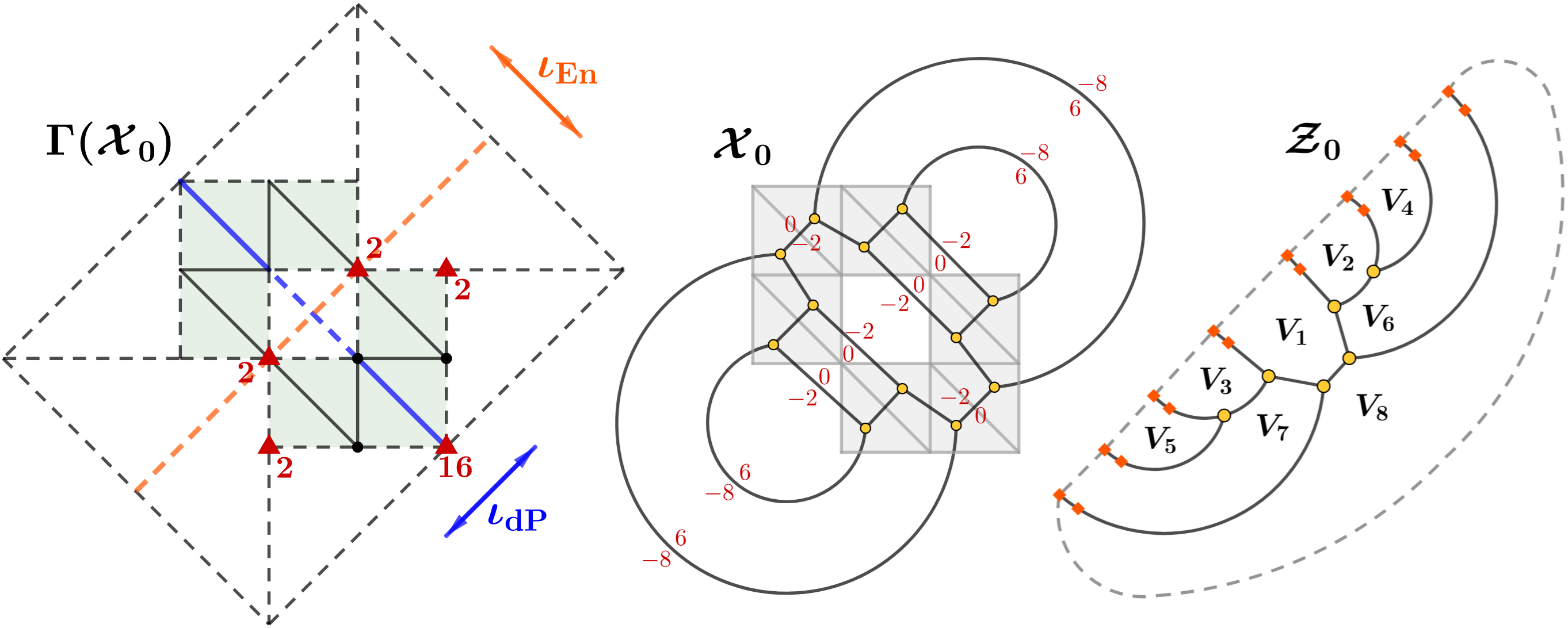
Figure 13. $B_{3}(\ell)$ and central fibers for $\ell=(2,0^{15},2,4,6,4,0,4)$.

The $\operatorname{IAS^{2}}$ is then admits two involutions, Enriques and del Pezzo, whose actions are shown in orange and blue, respectively. The corresponding Enriques and del Pezzo equators are shown in the respective colors. A triangulation into (green) lattice triangles is chosen, subordinate to both equators. The blue del Pezzo equator, with integer weight $2$, forms the integral-affine polarization $R_{\rm IA}$.

The middle image of Figure 13 depicts the corresponding Kulikov model ${\mathcal{X}}_{0}$ of Enriques K3 degeneration. Triple points ${\widetilde{T}}_{ijk}={\widetilde{V}}_{i}\cap{\widetilde{V}}_{j}\cap{\widetilde{V}}_{k}$ are depicted in yellow, double curves ${\widetilde{D}}_{ij}={\widetilde{V}}_{i}\cap{\widetilde{V}}_{j}$ are depicted in black. The self-intersection numbers

$${\widetilde{D}}_{ij}\big{|}_{{\widetilde{V}}_{i}}^{2}+{\widetilde{D}}_{ij}\big{|}_{{\widetilde{V}}_{j}}^{2}=-2$$

are written in red (suppressed when both equal $-1$). The faces, including an outer face, represent the components ${\widetilde{V}}_{i}$ with their anticanonical cycles ${\widetilde{D}}_{i}=\sum_{j}{\widetilde{D}}_{ij}$.

The righthand of Figure 13 depicts the dlt model. It consists of eight components $V_{i}$, $i=1,\dotsc,8$. Double loci and triple points are still depicted in black and yellow. Successive components along the image of the Enriques equator are

$$V_{1}\cup V_{2}\cup V_{4}\cup V_{6}\cup V_{8}\cup V_{7}\cup V_{5}\cup V_{3}\cup V_{1}$$

and the double curves between these two components contain two $A_{1}$-singularities of either containing surface, depicted by orange diamonds.

The double covers $({\widetilde{V}}_{6},{\widetilde{D}}_{6})\simeq({\widetilde{V}}_{7},{\widetilde{D}}_{7})$ are toric, isomorphic to a two-fold corner blowup of ${\mathbb{F}}_{6}$ as is $({\widetilde{V}}_{1},{\widetilde{D}}_{1})$, which is the blow-up of the four corners of an anticanonical square in ${\mathbb{P}}^{1}\times{\mathbb{P}}^{1}$.

The double covers $({\widetilde{V}}_{2},{\widetilde{D}}_{2})\simeq({\widetilde{V}}_{3},{\widetilde{D}}_{3})$ are the internal blow-ups of ${\mathbb{P}}^{1}\times{\mathbb{P}}^{1}$ at two points $p,q$ on opposite components of an anticanonical square. The Enriques involution acts in the corresponding toric coordinates by $(x,y)\mapsto(x^{-1},-y)$, and thus for this involution to lift to the internal blow-up, the two blow-up points must be interchanged: $y(p)=-y(q)$. This corresponds to choosing the involution anti-invariant periods on ${\mathcal{X}}_{0}$ for the unique $\times$-ed node at Cusp 3.

The double covers $({\widetilde{V}}_{4},{\widetilde{D}}_{4})\simeq({\widetilde{V}}_{5},{\widetilde{D}}_{5})$ are both isomorphic to ${\mathbb{F}}_{2}$. Finally, $({\widetilde{V}}_{8},{\widetilde{D}}_{8})$ is a minimal resolution of the $A_{15}$ surface of [AT21]. It is the $16$-fold internal blowup of ${\mathbb{F}}_{8}$ at $16$ points on a section $s$, $s^{2}=8$. These $16$ points are placed symmetrically with respect to an involution of $s$ and ${\mathbb{F}}_{8}$, giving rise to an Enriques involution on $({\widetilde{V}}_{8},{\widetilde{D}}_{8})$.

The divisor ${\mathcal{R}}_{{\mathcal{Z}}_{0}}\subset{\mathcal{Z}}_{0}$ is entirely supported on $V_{1}\cup_{D_{18}}V_{8}$ and has intersection number ${\mathcal{R}}_{{\mathcal{Z}}_{0}}\cdot D_{18}=1$. We have that $R_{1}^{2}=0$ and $R_{1}\subset V_{1}$ is the image of two fibers of a toric ruling on ${\widetilde{V}}_{1}$ while $R_{8}\subset V_{8}$ satisfies $R_{8}^{2}=8$ as it is the reduced image of the fixed locus ${\widetilde{R}}_{8}\subset{\widetilde{V}}_{8}$ satisfying ${\widetilde{R}}_{8}^{2}=16$.

The map to the stable model $(\overline{{\mathcal{Z}}}_{0},\epsilon\overline{{\mathcal{R}}}_{\overline{{\mathcal{Z}}}_{0}})$ contracts all components except $V_{1}$ and $V_{8}$ to points and contracts $V_{1}$ along a ruling, leaving the image of $V_{8}$ as the only component. The normalization

$$({\overline{V}}_{8},{\overline{D}}_{8}+\epsilon{\overline{R}}_{8})\simeq(\overline{{\mathcal{Z}}}_{0},\epsilon\overline{{\mathcal{R}}}_{\overline{{\mathcal{Z}}}_{0}})^{\nu}$$

has, as anticanonical boundary ${\overline{D}}_{8}\simeq{\mathbb{P}}^{1}$, which is self-glued in $\overline{{\mathcal{Z}}}_{0}$ along an involution fixing $0,\infty\in{\overline{D}}_{8}$. The singularities at $0,\infty\in{\overline{V}}_{8}$ are rather complicated.

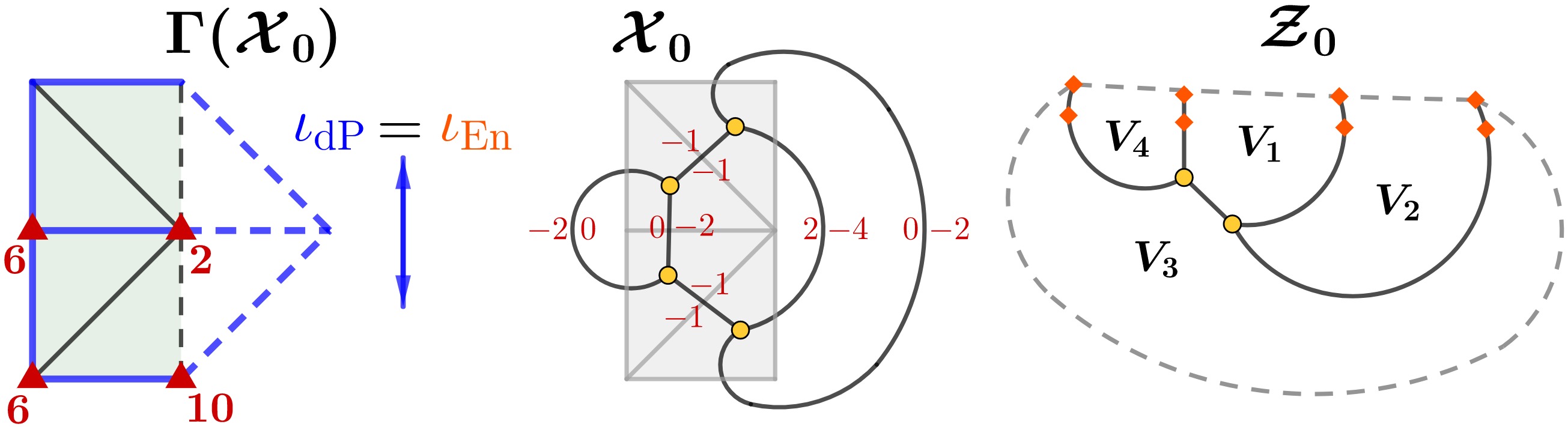
Figure 14. $B_{5}(\ell)$ and central fibers for $\ell=(0,0,2,0^{7},1,0^{3},1,0,0,0,2,0,2,6)$.

Example 4.14.

$B_{5}(0,0,2,0^{7},1,0^{3},1,0,0,0,2,0,2,6)$: Consider Cusp 5, whose folding symmetry is the same as $\iota_{\rm dP}$. This value of $\ell$ dictates that we should put $(2,0)$, $(-1,1)$, $(-1,0)$, $(0,-1)$ end-to-end, then perform a surgery of size $1$ along the edge $(-1,1)$, to construct $P(\ell)$. The corresponding sphere $B(\ell)$ is shown in Figure 14, together with a Kulikov and dlt model, following the conventions of Example 4.13.

There are four components $({\widetilde{V}}_{i},{\widetilde{D}}_{i})\subset{\mathcal{X}}_{0}$ of the Kulikov model, all of them preserved by the Enriques involution. Both $({\widetilde{V}}_{3},{\widetilde{D}}_{3})$ and $({\widetilde{V}}_{4},{\widetilde{D}}_{4})$ are corner blow-ups of $D_{4}$ involution pairs. The surface $({\widetilde{V}}_{1},{\widetilde{D}}_{1})$ is the internal blow-up at points on two opposite fibers of an anticanonical square in ${\mathbb{F}}_{2}$ and the Enriques involution interchanges the blow-up points. Finally, $({\widetilde{V}}_{2},{\widetilde{D}}_{2})$ is a corner blow-up of a $D_{8}$ involution pair. We have ${\widetilde{R}}_{1}^{2}=0$, ${\widetilde{R}}_{2}^{2}=8$, ${\widetilde{R}}_{3}^{2}={\widetilde{R}}_{4}^{2}=4$.

The components of the stable limit of Enriques surfaces $({\overline{V}}_{3},{\overline{D}}_{3}+\epsilon{\overline{R}}_{3})\simeq({\overline{V}}_{4},{\overline{D}}_{4}+\epsilon{\overline{R}}_{4})$ are denoted $D_{4}:2=\kern-2.0pt\phantom{.}_{2}\kern-1.0pt^{\prime}\kern-2.0ptB_{2}^{-}$ and $({\overline{V}}_{2},{\overline{D}}_{2}+\epsilon{\overline{R}}_{2})$ is denoted by $D_{8}:2=\kern-2.0pt\phantom{.}_{2}\kern-1.0pt^{\prime}\kern-2.0ptB_{4}^{-}$ in Section 6, where these surfaces are described further. Only $V_{1}$ is contracted (along a ruling) in the stable limit $\overline{{\mathcal{Z}}}_{0}$.

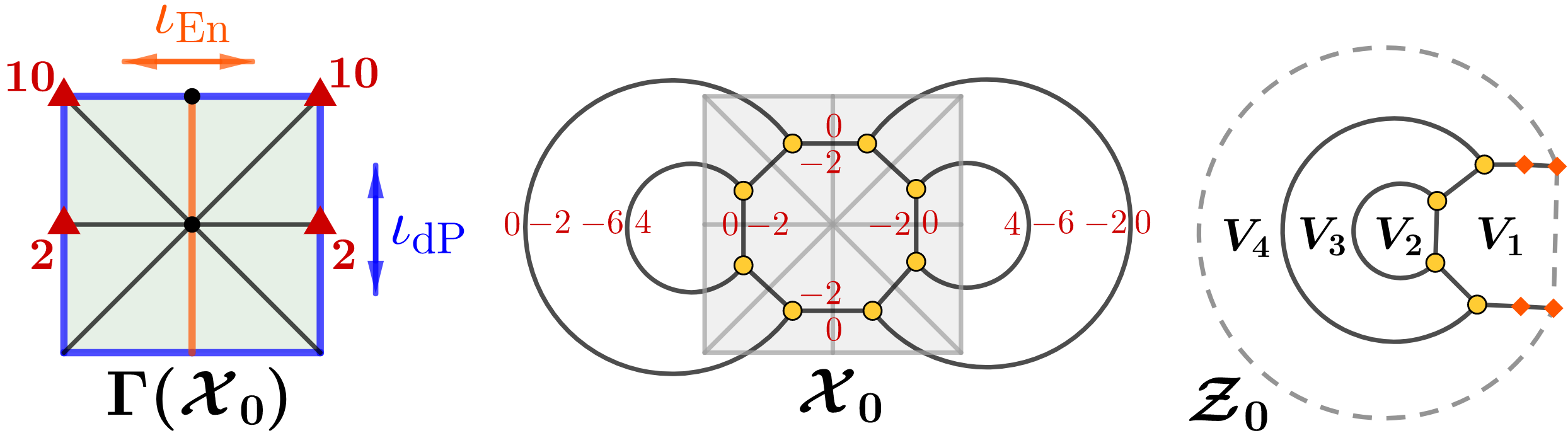
Figure 15. $B_{2}(\ell)$ and central fibers for $\ell=(0,1,0^{7},2,0^{7},1,0)$.

Example 4.15.

$B_{2}(0,1,0^{7},2,0^{7},1,0)$: Note here that since we are at Cusp 2, $\ell\in({\mathbb{Z}}_{\geq 0})^{19}$. To form ${\overline{P}}(\ell)$, we put $(0,1)$, $(-2,0)$, $(0,-1)$ end-to-end, and then close the base of the polygon by a horizontal line. No Symington surgeries of positive size are made, so $P(\ell)={\overline{P}}(\ell)$. We glue to get $B(\ell)$ as in Figure 15. Even though the central horizontal segment is fixed by $\iota_{{\rm dP},{\rm IA}}$ it does not form part of the support of $R_{\rm IA}$, see Section 4.2.

Then ${\widetilde{V}}_{2}$ and ${\widetilde{V}}_{3}$ are each two disjoint copies of $V_{2}$ and $V_{3}$. $(V_{2},D_{2})\simeq({\mathbb{F}}_{1},{\widehat{L}}+C)$ where ${\widehat{L}}$ is the strict transform of a line in ${\mathbb{P}}^{2}$ and $C$ is a conic. The surface $(V_{3},D_{3})$ is, up to two corner blow-ups, the $D_{8}$ involution pair as in Example 4.14, but since $({\widetilde{V}}_{3},{\widetilde{D}}_{3})$ is two disjoint copies of such, there is no period-theoretic restriction. Finally, $(V_{1},D_{1})$ and $(V_{4},D_{4})$ form the image of the Enriques equator. They are both quotients of smooth toric surfaces by an involution $(x,y)\mapsto(x^{-1},-y)$.

Only $V_{3}$ survives as a component $({\overline{V}}_{3},{\overline{D}}_{3}+\epsilon{\overline{R}}_{3})$. The double locus ${\overline{D}}_{3}\simeq{\mathbb{P}}^{1}\cup{\mathbb{P}}^{1}$ is a banana curve. In the stable model $\overline{{\mathcal{Z}}}_{0}$, each ${\mathbb{P}}^{1}\subset{\overline{D}}_{2}$ is self-glued by an involution fixing the two nodes in ${\overline{D}}_{3}$. We have $({\overline{R}}_{3})^{2}=8$.

Example 4.16.

$B_{4}(0^{6},1,0^{7},1,0^{5},2,2)=B_{1}(0,0,1,0^{7},1,0^{9},2,2)$. This is the Type II ray corresponding to the $1$-cusp with label $41$, so it occurs as a limit of $\operatorname{IAS^{2}}$ at either Cusp 1 or 4. The dual complex $\Gamma({\mathcal{X}}_{0})$ is a segment of length one and the Enriques involution flips the segment (this means that, strictly speaking, the Enriques equator is not a sub-simplicial complex of $\Gamma({\mathcal{X}}_{0})$, as we usually require). The surface ${\mathcal{X}}_{0}={\widetilde{V}}_{1}\cup_{E}{\widetilde{V}}_{2}$ is the union of two copies of the same ${\widetilde{D}}_{8}$ involution pair, glued with a twist by $2$-torsion along the elliptic curves $E\in|-K_{{\widetilde{V}}_{i}}|$.

The quotient ${\mathcal{Z}}_{0}$ is then a non-normal surface with ${\mathcal{Z}}_{0}^{\nu}\simeq({\widetilde{V}}_{1},E)$, and the normalization map glues $E$ to itself by the $2$-torsion translation. We have $\overline{{\mathcal{Z}}}_{0}={\mathcal{Z}}_{0}$.

5. Toroidal, semitoroidal, and KSBA compactifications

5.1. Toroidal compactification for the Coxeter fans

In Section 3.4 we reviewed the basic results of [Vin72, Vin75] on reflection groups acting on hyperbolic lattices. Now we recall applications of this theory to toroidal compactifications.

Let $\Lambda$ be a hyperbolic lattice of rank $r$ and signature $(1,r-1)$, and let ${\mathcal{C}}$ be the positive cone, one of the two halves of the set $\{v\in\Lambda_{\mathbb{R}}\mid v^{2}>0\}$. In the applications to (semi)toroidal compactifications, instead of the closure $\overline{{\mathcal{C}}}$ one operates with the rational closure $\overline{{\mathcal{C}}}_{\mathbb{Q}}$, obtained by adding only rational vectors at infinity.

Let $W$ be a group acting on $\Lambda$, generated by reflections in a set of vectors of $\Lambda$. Its fundamental domain is

$${\mathfrak{C}}=\{v\in\overline{{\mathcal{C}}}\mid\alpha_{i}\cdot v\geq 0\}$$

for a set of simple roots $\alpha_{i}$ with $\alpha_{i}^{2}<0$ which is encoded in a Coxeter diagram $G$. The chamber ${\mathfrak{C}}$ can be identified with a polyhedron $P$ in the hyperbolic space ${\mathbb{P}}{\mathcal{C}}$. The vectors with $v^{2}=0$ are treated as points at infinity of ${\mathbb{P}}{\mathcal{C}}$.

The subgroup $O^{+}(\Lambda)$ of the isometry group $O(\Lambda)$ is the subgroup of index $2$ that preserves ${\mathcal{C}}$. One has $O^{+}(\Lambda)=S.W$, where $S$ is a subgroup of symmetries of $P$.

Definition 5.1.

The Coxeter semifan ${\mathfrak{F}}_{\rm cox}$ is the semifan with support $\overline{{\mathcal{C}}}_{\mathbb{Q}}$ whose maximal cones are chambers of $W$, i.e. ${\mathfrak{C}}$ and its $W$-images.

It is a fan iff $P$ has finite volume, which is equivalent to $W$ having finite index in $O(\Lambda)$. If this condition is satisfied then the faces of ${\mathfrak{C}}$ are of two types:

1. Type II rays ${\mathbb{R}}_{\geq 0}v$ generated by vectors with $v^{2}=0$ on the boundary of $\overline{{\mathcal{C}}}_{\mathbb{Q}}$. These are in bijection with the maximal parabolic subdiagrams of $G$.

2. Type III cones. These are in bijection with elliptic subdiagrams of $G$.

By [AE22, Sec. 3B] the moduli space $F_{(2,2,0)}$ admits a toroidal compactification ${\overline{F}}_{(2,2,0)}^{\rm cox}$ defined by the collection of fans ${\mathfrak{F}}_{\rm cox}^{\rm dP}=\{{\mathfrak{F}}_{r}(18,0,0),{\mathfrak{F}}_{r}(18,2,0)\}$, one for each $0$-cusp. These fans are Coxeter fans for the hyperbolic lattices $(18,0,0)_{1}$, $(18,2,0)_{1}$ for the full reflection groups $W_{r}$, generated by reflections in the $(-2)$-roots and in the $(-4)$-roots of divisibility $2$. The Coxeter diagrams $G_{r}(18,0,0)$ and $G_{r}(18,2,0)$ are given in Figure 5.

By Lemma 2.8 there is an immersion $j\colon F_{\rm En,2}\to F_{(2,2,0)}$ whose image is a Noether-Lefschetz locus in $F_{(2,2,0)}$. The normalization of the closure of $j(F_{\rm En,2})$ in ${\overline{F}}_{(2,2,0)}^{\rm cox}$ is then a toroidal compactification ${\overline{F}}_{\rm En,2}^{\rm cox}$ for the fans $\{{\mathfrak{F}}^{k}_{\rm cox}\}_{k=1,2,3,4,5}$, one for each of $0$-cusp of $F_{\rm En,2}$. The fans ${\mathfrak{F}}^{k}_{\rm cox}$ are the intersections of the above fans ${\mathfrak{F}}_{r}$ in the lattices ${\overline{T}}_{\rm dP}=(18,0,0)_{1}$ and $(18,2,0)_{1}$ with the sublattices ${\overline{T}}_{\rm En}=(10,10,0)_{1}$ and $(10,8,0)_{1}$, as in Section 3. By Lemma 3.8 and Corollary 3.12 these five fans are the Coxeter fans for the folded Coxeter diagrams $G_{r}^{k}$ of Figures 7, 8. By [Ste91] the induced groups acting on $e^{\perp}/e$ are of the form $\Gamma_{k}=\operatorname{Aut}(G_{r}^{k})\ltimes W(G_{r}^{k})$

Lemma 5.2.

For $k=1,2,3,4,5$, the numbers of Type II + Type III rays in ${\mathfrak{F}}^{k}_{\rm cox}/\Gamma_{k}$ are $4+4$, $2+8$, $3+15$, $4+12$, $5+17$. The toroidal compactification ${\overline{F}}_{\rm En,2}^{\rm cox}$ has $9+56=65$ Type II + Type III divisors.

Proof.

Direct enumeration of maximal parabolic and elliptic subdiagram of rank $9$ in the Coxeter diagrams $G^{k}_{r}$. Type II divisors correspond to curves in ${\overline{F}}_{\rm En,2}^{\rm BB}$ passing through several $0$-cusps, so each of them corresponds to several rays in ${\mathfrak{F}}^{k}/\Gamma_{k}$. ∎

5.2. Semitoroidal compactification for the generalized Coxeter fans

Looijenga’s semitoric, or semitoroidal compactifications of Type IV domains [Loo03] generalize toroidal compactifications in several ways. By [AE23, Thm. 7.18] these are the normal compactifications dominating the Baily-Borel compactification and dominated by some toroidal compactification. They are defined by collections of compatible semifans, one for each Baily-Borel $0$-cusp. The data for the $1$-cusps is then uniquely determined. The cones in semifans have rational generators but, unlike in fans, there could be infinitely many generators, and the stabilizer groups of the Type III cones may be infinite.

The generalized Coxeter semifans were defined in [AET23, Section 4D] using the Wythoff construction [Cox35], as follows. As above, let $W$ be a reflection group with a fundamental chamber ${\mathfrak{C}}$ and $G=\{\alpha_{i}\}$ be the corresponding Coxeter diagram. Divide the vertices of $G$ into two complementary sets $I\sqcup J$ of relevant and irrelevant roots. Let $W_{\rm irr}$ be the subgroup of $W$ generated by the irrelevant roots and let ${\mathfrak{C}}_{\rm gen}=\cup_{h\in W_{\rm irr}}h.{\mathfrak{C}}$ The maximal dimensional cones in the semifan ${\mathfrak{F}}_{\rm gen}$ are the chamber ${\mathfrak{C}}_{\rm gen}$ and its images under $W$. Another way to describe ${\mathfrak{F}}_{\rm gen}$ is that it is the coarsening of the Coxeter fan ${\mathfrak{F}}_{\rm cox}$ obtained by removing the faces of the form $\cap\alpha_{j}^{\perp}\cap{\mathfrak{C}}$ in which $\{\alpha_{j},\ j\in J^{\prime}\subset J\}$ is a collection of irrelevant roots.

In [AE22, Sec. 9A] the authors defined a specific semitoroidal compactification of the moduli space $F_{(2,2,0)}$ by the collection ${\mathfrak{F}}_{\rm ram}=\{{\mathfrak{F}}_{\rm ram}(18,0,0),{\mathfrak{F}}_{\rm ram}(18,2,0)\}$ of two semifans. (Here, ram stands for the ramification divisor.) These are the generalized Coxeter semifans for the Coxeter diagrams of Figure  5 in which the irrelevant roots are those that do not lie on the boundary of the square, resp. the triangle, numbered respectively $0$–$15$ and $2$–$18$. The main theorem of [AE22] for the moduli space $F_{(2,2,0)}$ says that the normalization of the KSBA moduli compactification ${\overline{F}}_{(2,2,0)}$ for the pairs $(X,\epsilon R)$ is this semitoroidal compactification.

Definition 5.3.

The collection of semifans ${\mathfrak{F}}=\{{\mathfrak{F}}^{k}\}_{k=1,2,3,4,5}$, one for each $0$-cusp of $F_{\rm En,2}$ is defined by intersecting the semifans ${\mathfrak{F}}_{\rm ram}({\overline{T}}_{\rm dP})$ for ${\overline{T}}_{\rm dP}=(18,0,0)_{1}$, $(18,2,0)_{1}$ with the subspace ${\overline{T}}_{\rm En}=(10,10,0)_{1}$ and $(10,8,0)_{1}$ as in Section 3.

Definition 5.4.

In each of the folded Coxeter diagrams of Figures 7, 8, call a root irrelevant if it is obtained by folding of an irrelevant root in Figure 5, i.e. a root which does not lie on the boundary of the square, resp. the triangle.

Lemma 5.5.

The semifans $\{{\mathfrak{F}}^{k}\}_{k=1,2,3,4,5}$ are the generalized Coxeter fans for the folded Coxeter diagrams of Figures 7, 8 with the irrelevant roots of Definition 5.4.

Proof.

By Lemma 3.8, for a root $\alpha$ of ${\overline{T}}_{\rm dP}$, if $\alpha^{\perp}$ intersects the interior of the positive cone ${\mathcal{C}}$ in ${\overline{T}}_{\rm En}$ then $\alpha^{\perp}\cap{\mathcal{C}}=\alpha_{J}^{\perp}\cap{\mathcal{C}}$ for the folded root $\alpha_{J}$. By definition, irrelevant roots fold to irrelevant roots. Thus, the fans ${\mathfrak{F}}^{k}$ are obtained from the Coxeter fans ${\mathfrak{F}}^{k}_{\rm cox}$ by removing the faces of the form $\cap\alpha_{j}^{\perp}\cap{\mathfrak{C}}$ in which $\{\alpha_{j},\ j\in J^{\prime}\subset J\}$ is a collection of irrelevant folded roots. So these are the generalized Coxeter semifans as stated. ∎

Lemma 5.6.

The semifans ${\mathfrak{F}}^{k}$ are fans for $k=2,4$ and are not fans for $k=1,3,5$.

Proof.

Indeed, for $k=2$, resp. $k=4$, the irrelevant subgroup $W_{\rm irr}=S_{2}$, resp. $S_{2}^{2}$, is finite. For the other $0$-cusps the groups $W_{\rm irr}$ are infinite, the cones ${\mathfrak{C}}_{k}$ have infinitely many generators, and the corresponding polyhedra have infinite volumes. ∎

Lemma 5.7.

The semitoroidal compactification of $F_{\rm En,2}$ defined by the collection of semifans $\{{\mathfrak{F}}^{k}\}_{k=1,2,3,4,5}$ is toroidal over the $0$-cusps $2$ and $4$ and the $1$-cusps which are adjacent to them, and over $1$-cusp $35$. It is strictly semitoroidal over the remaining cusps.

Proof.

By Lemma 5.6, this semitoroidal compactification is toroidal over the cusps 2 and 4 and so also over the $1$-cusps adjacent to it. In general, the definition of the generalized Coxeter semifan above implies that the semitoroidal compactification is toroidal over a $1$-cusp exactly when the corresponding maximal parabolic diagram does not have a connected component consisting entirely of irrelevant vertices. Examining Figure 10 shows that in addition to the $1$-cusps adjacent to the $0$-cusps 2 and 4 there is just one more, for the $1$-cusp $35$. This completes the proof. ∎

Lemma 5.8.

For $k=1,2,3,4,5$, the numbers of Type II + Type III divisors at the cusps of the semitoroidal compactification ${\overline{F}}_{\rm En,2}^{\mathfrak{F}}$ are $2+0$, $2+7$, $2+7$, $4+7$, $3+0$, for a total of $6+21=27$ divisors.

Proof.

This is obtained by removing from the list of subgraphs in Lemma 5.2 the graphs containing a connected component consisting of irrelevant vertices. ∎

5.3. The main theorem

By Section 2.4 there exists a compact moduli space ${\overline{F}}_{\rm En,2}$ whose points correspond to the pairs $(Z,\epsilon R_{Z})$ of Enriques surfaces with numerical polarization of degree $2$ and their KSBA stable limits, for any $0<\epsilon\ll 1$. This is the closure of $F_{\rm En,2}$ in the KSBA moduli space of stable pairs.

Theorem 5.9.

The normalization of ${\overline{F}}_{\rm En,2}$ is semitoroidal for the collection of semifans $\{{\mathfrak{F}}^{k}\}_{k=1,2,3,4,5}$ of Section 5.2. It is toroidal over the $0$-cusps $2$ and $4$, the $1$-cusps which are adjacent to them, and over $1$-cusp $35$. It is strictly semitoroidal over the remaining cusps.

Proof.

The main theorem of [AE23] is that the normalization of the KSBA compactification of K3 pairs $(X,\epsilon R)$ for a recognizable divisor $R$ is semitoroidal and by [AEH21] the ramification divisor is recognizable. The main theorem of [AE22] for $F_{(2,2,0)}$ is that this semifan is the ramification semifan ${\mathfrak{F}}_{\rm ram}$ of Section 5.2.

Consider the universal family $({\mathcal{X}},\epsilon{\mathcal{R}})\to{\overline{F}}_{(2,2,0)}$ of KSBA-stable pairs over the compactified moduli stack. Denote the closure of the image of $F_{\rm En,2}$ in ${\overline{F}}_{(2,2,0)}$ by $B$. Then, the pullback of the universal family $({\mathcal{X}}_{B},\epsilon{\mathcal{R}}_{B})\to B$ is a family whose general fiber is a pair $(X,\epsilon R)$ of an Enriques K3 surface with the ramification divisor $R$ of the del Pezzo involution. By uniqueness of KSBA-stable limits, the Enriques involution on the general fiber extends to an involution on the universal family $({\mathcal{X}}_{B},\epsilon{\mathcal{R}}_{B})$. Taking the quotient gives a family $({\mathcal{Z}},\epsilon{\mathcal{R}}_{{\mathcal{Z}}})\to B$ over a compact base, extending the universal family of Enriques surfaces $(Z,\epsilon R_{Z})$ with divisor.

By Lemma 2.8, the normalization $B^{\nu}$ of $B$ is a compactification of $F_{\rm En,2}$ admitting a universal family of pairs. So we have a classifying morphism $B^{\nu}\to{\overline{F}}_{\rm En,2}$. Furthermore, $B^{\nu}$ is simply the semitoroidal compactification of the Noether-Lefschetz locus $B$, induced by the semifan ${\mathfrak{F}}_{\rm ram}$ which gives the normalization ${\overline{F}}_{(2,2,0)}^{\nu}$. This gives a family of KSBA stable pairs over the induced compactification ${\overline{F}}_{\rm En,2}$, whose normalization by Section 5.2 is the compactification ${\overline{F}}_{\rm En,2}^{\mathfrak{F}}$ for the collection of semifans ${\mathfrak{F}}=\{{\mathfrak{F}}^{k}\}_{k=1,2,3,4,5}$.

To prove the first statement, it remains to show that $B^{\nu}\to{\overline{F}}_{\rm En,2}$ is a finite map. Equivalently, we do not lose moduli when we quotient a stable K3 pair $(X,\epsilon R)$ by $\iota_{\rm En}$. By [AE23, Thm. 7.18], the normalization of ${\overline{F}}_{\rm En,2}$ is given by some semifan coarsening ${\mathfrak{F}}^{k}$ and so it suffices to prove that the maximal cones of this semifan are the same as the maximal cones ${\mathfrak{F}}^{k}$.

The explicit description of Kulikov and stable models from Proposition 4.8 and Corollary 4.9 imply the following fact: a degeneration of $(Z,\epsilon R_{Z})$ has a maximal number of double curves if and only if $(X,\epsilon R)$ does. But if the normalization of ${\overline{F}}_{\rm En,2}$ were given by any strict coarsening of $\{{\mathfrak{F}}^{k}\}$, there would be some codimension one cone of some ${\mathfrak{F}}^{k}$ that parameterized a $1$-dimensional family of non-maximal pairs $(X,\epsilon R)$, whose Enriques quotients $(Z,\epsilon R_{Z})$ had the maximal number of double curves. This is impossible, so we conclude the first statement.

The last statement follows by Lemma 5.7. ∎

6. ABCDE surfaces

The paper [AT21] classified the surfaces which may appear as irreducible components of KSBA stable degenerations of K3 surfaces with a non-symplectic involution $(X,\iota)$ for the pairs $(X,\epsilon R)$, where $R$ is a component of genus $g\geq 2$ of the ramification divisor of the double cover $X\to X/\iota$. In particular, the irreducible components of stable pairs $(X,\epsilon R)$ in [AET23, AE22] are all of these types. The surfaces appearing in Type III degenerations naturally correspond to Dynkin diagrams $A_{n}$, $D_{n}$, $E_{n}$, and those appearing in Type II degenerations to the affine ${\widetilde{A}}_{n}$, ${\widetilde{D}}_{n}$, ${\widetilde{E}}_{n}$ diagrams. Both come with decorations addressing parity and some extra data, as in Section 6.2 below.

On the other hand, it is well known that the non simply laced Dynkin diagrams of BCFGH types can be naturally described by “folding” ADE diagrams by automorphisms. After recalling the ADE surfaces relevant to this paper, we define new B and C type surfaces obtained from them as quotients by involutions.

The surfaces in [AT21] come in pairs $\pi\colon(X,D+\epsilon R)\to(Y,C+\textstyle\frac{1+\epsilon}{2}B)$, fully analogous to Diagram (1) in the introduction. Here:

1. $(Y,C)$ is a log del Pezzo pair of index $2$ with reduced boundary $C$ and a nonempty nonklt locus. The divisor $B\in|-2(K_{Y}+C)|$ is ample Cartier, and the pair $(Y,C+\textstyle\frac{1+\epsilon}{2}B)$ is KSBA stable; in particular it is log canonical.

2. $\pi\colon X\to Y$ is the index-$1$ cover for $K_{Y}+C$. Explicitly, $X=\operatorname{Spec}{\mathcal{A}}$, where ${\mathcal{A}}={\mathcal{O}}_{Y}\oplus{\mathcal{O}}_{Y}(K_{Y}+C)$ is an ${\mathcal{O}}_{Y}$-algebra with the multiplication defined by an equation of $B$. One has $K_{X}+D\sim 0$, $R=\frac{1}{2}\pi^{*}(B)$ is ample, the pair $(X,D+\epsilon R)$ is KSBA stable and it has a nonempty nonklt locus.

By the Riemann-Hurwitz formula, one has

(7) $$K_{X}+D+\epsilon R=\pi^{*}\left(K_{Y}+C+\textstyle\frac{1+\epsilon}{2}B\right)$$

By [AT21, Lemma 2.3], the pairs $(Y,C+\textstyle\frac{1+\epsilon}{2}B)$ and $(X,D+\epsilon R)$ are in a one-to-one correspondence. To distinguish them we will call the former del Pezzo ADE surfaces and the latter anticanonical ADE surfaces.

6.1. Type III ADE surfaces

The only ADE surfaces needed in this paper are the ones that appear on the boundary of the KSBA compactification ${\overline{F}}_{(2,2,0)}$. They are described in detail in the last section of [AE22]. Most of them are easy: they are hypersurfaces in projective toric varieties in a way very similar to the construction in Section 2.1.

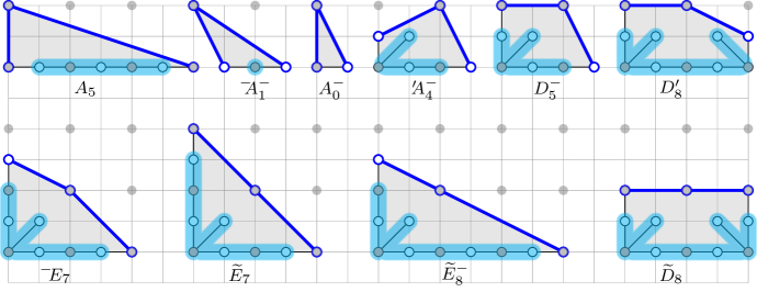
Figure 16. Some ADE surfaces

As an example, consider one of the lattice polytopes $Q$ in Figure 16 with an ADE Dynkin diagrams fitted into it. The polytopes are in ${\mathbb{Z}}^{2}$, and the gray dots indicate the sublattice $2{\mathbb{Z}}^{2}$. The Type III polytopes for the ordinary elliptic ADE diagrams have a distinguished vertex with two bold blue sides emanating from it. In the Type II polytopes for the extended ${\widetilde{D}}{\widetilde{E}}$ diagram there is a distinguished point in the interior of the bold blue segment. Together with the ends of this segment, it makes three special vertices.

By the standard construction, one associates to $Q$ a toric variety $V_{Q}$ with an ample line bundle $L_{Q}$. Let us define a section of $L_{Q}$ as the following sum of monomials in $Q\cap{\mathbb{Z}}^{2}$. For Type III, each of the three special vertices above gets coefficient $1$. The coefficients of the vertices in the highlighted Dynkin diagrams are arbitrary numbers $a_{i}\in{\mathbb{C}}$. The other coefficients are zero. Concretely:

1. $f=(1+y^{2}+x^{6})+\sum_{i=1}^{5}a_{i}x^{i}$

2. $f=(x+y^{2}+x^{3})+a_{1}x^{2}$

3. $f=1+y^{2}+x$

4. $f=(y+x^{2}y^{2}+x^{3})+a_{1}xy+a_{2}+a_{3}x+a_{4}x^{2}$

5. $f=(y^{2}+x^{2}y^{2}+x^{3})+a_{1}xy+a_{2}y+a_{3}+a_{4}x+a_{5}x^{2}$

6. $f=(y^{2}+x^{2}y^{2}+x^{4}y)+a_{1}xy+a_{2}y+\sum_{i=0}^{4}a_{i+3}x^{i}+a_{8}x^{3}y$

7. $f=(y^{3}+x^{2}y^{2}+x^{4})+a_{1}xy+a_{2}y^{2}+a_{3}y+a_{4}+a_{5}x+a_{6}x^{2}+a_{7}x^{3}$

The corresponding del Pezzo ADE surface is the toric variety $Y=V_{Q}$ together with the boundary $C=C_{1}+C_{2}$ for the two blue sides, and the divisor $B$ is $(f)$. Combinatorially the condition $B\sim-2(K_{Y}+C)$ is equivalent to the condition that the other sides of $Q$ have lattice distance $2$ from the distinguished point.

We now put these polytopes in ${\mathbb{Z}}^{2}\times 0\subset{\mathbb{Z}}^{3}$. Let $p_{0}$ be the position of the distinguished vertex, we then add another vertex at the point $p_{0}+(0,0,2)$ to which we associate the monomial $z^{2}$. Let $P$ be the pyramid with the apex at the new vertex and with base $Q$. Associated to it we have a $3$-dimensional polarized toric variety $(V_{P},L_{P})$ and a section $z^{2}+f$ of $L_{P}$. An anticanonical ADE surface $X$ is the zero set of this section, so it is a hypersurface in $V_{P}$. It comes with a del Pezzo involution $\iota_{{\rm dP}}\colon(x,y,z)\to(x,y,-z),$ the quotient map is $\pi\colon X\to X/\iota_{{\rm dP}}=Y$, the boundary is $D=\pi^{-1}(C)$, and the ramification divisor is $R=\pi^{-1}(B)$.

Varying the free coefficients $a_{i}$ we get a family over ${\mathbb{C}}^{n}$, where $n$ is the rank of the Dynkin diagram. This ${\mathbb{C}}^{n}$ is the quotient of the algebraic torus $\operatorname{Hom}(\Lambda^{*},{\mathbb{C}}^{*})\simeq({\mathbb{C}}^{*})^{n}$ by the Weyl group $W(\Lambda)$ for the ADE root lattice $\Lambda$ with the weight lattice $\Lambda^{*}$. So it naturally comes from a family over a torus.

6.2. Decorations

Because of $z^{2}$ and the double cover, the vertices in $2{\mathbb{Z}}^{2}\subset{\mathbb{Z}}^{2}$ are clearly distinguished; let’s call them even. When the end of a bold blue edge is even, this edge is long, of lattice length $2$. Then we use no decorations. When this end is odd, the edge is short, of lattice length $1$. To indicate that it is short, we use a minus or a prime sign. We also use primes to distinguish shapes where the long leg pokes into the interior of $Q$.

The classification of del Pezzo ADE surfaces $(Y,C+\textstyle\frac{1+\epsilon}{2}B)$ in [AT21] is divided into pure and primed shapes. The surfaces for the pure shapes are all toric. The surfaces for some of the primed shapes are toric, but not in general. They are obtained from pure shapes by making a blow up at a point $x\in D\cap R$ on $X$, resp. a weighted blowup at a point $y\in C\cap B$ in $Y$. For each side $D_{1},D_{2}$, the set $D_{i}\cap R$ is either a single point (if the side is short) or two points (if it is long). E.g. priming $A_{n}$ on a long side once gives $A^{\prime}_{n}$ and twice gives $A^{\prime\prime}_{n}$. Priming $A^{-}_{n}$ on a short side is denoted by $A^{+}_{n}$.

The blow up disconnects $D_{i}$ from $R$ at that point. If all points in $D_{i}\cap R$ are blown up, for the strict preimages we have $D^{\prime}_{i}\cdot R^{\prime}=0$. In this case the linear system $|mR^{\prime}|$ for $m\gg 0$ contracts $D^{\prime}_{i}$ and the corresponding ADE surface has fewer boundary components. Thus, the surfaces e.g. for the shapes $A^{\prime\prime}_{n}$ and $A^{+}$ have only one boundary component, and for the shapes $\kern-2.0pt\phantom{.}^{\prime\prime}\kern-2.0pt\kern-1.0ptA_{n}^{\prime\prime}$, $\kern-2.0pt\phantom{.}^{\prime\prime}\kern-2.0pt\kern-1.0ptA_{n}^{+}$, $\raise 0.65pt\hbox{$\kern-2.0pt\phantom{.}^{+}$}\kern-4.0ptA_{n}^{+}$ have zero boundary components.

6.3. Type II ADE surfaces

The construction for the Type II polytopes is similar. The ends of the bold blue edge have coefficients $1$ in $f$, and the distinguished interior point has coefficient $\lambda\in{\mathbb{C}}$. For clarity, in Figure 16 one has

1. $f=(y^{4}+\lambda x^{2}y^{2}+x^{4})+a_{1}xy+a_{2}y^{3}+a_{3}y^{2}+a_{4}y+a_{5}+a_{6}x+a_{7}x^{2}+a_{8}x^{3}$

2. $f=(y^{3}+\lambda x^{2}y^{2}+x^{6})+a_{1}xy+a_{2}y^{2}+a_{3}y+\sum_{i=0}^{5}a_{4+i}x^{i}$

3. $f=(y^{2}+\lambda x^{2}y^{2}+x^{4}y^{2})+a_{1}xy+a_{2}x^{3}y+a_{4}x^{4}y+\sum_{i=0}^{4}a_{i+5}x^{i}$

The coefficients for the nodes of the extended Dynkin diagram are arbitrary numbers $a_{i}\in{\mathbb{C}}$, not all of them zero, and they are now treated as homogeneous coordinates of weight equal to the lattice distance from the bold blue edge. Thus, for a fixed $\lambda$ one gets a family of sections $z^{2}+f$ of $L_{P}$ and a family of anticanonical KSBA stable pairs $(X,D+\epsilon R)$ parameterized by a weighted projective space. For ${\widetilde{E}}_{7}$ it is ${\mathbb{P}}(1^{2},2^{3},3^{2},4)$, for ${\widetilde{E}}_{8}$ it is ${\mathbb{P}}(1,2^{2},3^{2},4^{2},5,6)$, and for ${\widetilde{D}}_{2n}$ it is ${\mathbb{P}}(1^{4},2^{2n-3})$. The restriction of $z^{2}+f$ to the divisor corresponding to the bold blue line gives a double cover of ${\mathbb{P}}^{1}$ which is an elliptic curve. Varying $\lambda$ we get a family of ${\widetilde{A}}{\widetilde{D}}{\widetilde{E}}$ surfaces parameterized by a bundle of weighted projective spaces over the $j$-line. This is the same bundle of weighted projective spaces that appeared in [Loo76, Pin77, Loo78].

The ${\widetilde{A}}_{2n-1}$ surfaces do not directly correspond to polytopes. These surfaces are double covers of cones over elliptic curves branched in a bisection. The easiest description, closest to toric is to use the Tate curve. For each $i\in{\mathbb{Z}}_{2n}$ define the theta function $\theta_{i}$ as the formal power series

$$\theta_{i}=\sum_{k\equiv i\,({\rm mod\ }{2n})}q^{k(k-1)/2}x^{k}$$

It converges for any $q\in{\mathbb{C}}^{*}$ with $|q|<1$ and defines a section of $L^{2}$, where $L$ is an ample line bundle of degree $n$ on the elliptic curve $E_{q}={\mathbb{C}}^{*}/q^{{\mathbb{Z}}}$. For any $c_{i}\in{\mathbb{C}}$ not all zero, $g(x)=\sum c_{i}\theta_{i}$ is a nonzero section of $L^{2}$ and $f(x,y)=y^{2}+g(x)$ is a section on the square of the tautological line bundle on ${\widetilde{Y}}={\mathbb{P}}({\mathcal{O}}\oplus L)$. It also defines a section of a line bundle on the surface $Y$ that is a cone over $E$, obtained by contracting an exceptional section of ${\widetilde{Y}}$. Finally, $z^{2}+f(x,y)$ defines a double cover $X\to Y$ and the covering involution $\iota_{{\rm dP}}$ is $(x,y,z)\to(x,y,-z).$

6.4. Anticanonical ADE surfaces with two commuting involutions

Let $(X,D)$ be a log canonical pair with $K_{X}+D\sim 0$. Pick a generator $\omega$ of the space $H^{0}({\mathcal{O}}(K_{X}+D))={\mathbb{C}}$. Just as for K3 surfaces, an involution $\iota$ is called symplectic if $\iota^{*}\omega=\omega$ and nonsymplectic if $\iota^{*}\omega=-\omega$. By looking at a local equation $dx\wedge\frac{dy}{y}$ of $\omega$ near the boundary, it is easy to see that for a nonsymplectic involution the quotient map $X\to X/\iota$ is not ramified along any irreducible component of $D$.

Proposition 6.1.

Let $\pi\colon(X,D+\epsilon R)\to(Y,C+\textstyle\frac{1+\epsilon}{2}B)$ be the anticanonical and del Pezzo ADE surfaces, and $\iota_{{\rm dP}}$ be the anticanonical involution such that $Y=X/\iota_{{\rm dP}}$. Suppose that $\iota_{{\rm En}}\colon X\to X$ is another nonsymplectic involution commuting with $\iota_{{\rm dP}}$ such that $\iota_{{\rm dP}}$ and the induced involution $\tau\colon Y\to Y$ both have finite fixed sets. Then there exists a diagram of log canonical pairs

(8)

in which

1. $\psi\colon X\to Z$ is the quotient by $\iota_{{\rm En}}$ and $\psi^{\prime}\colon X\to Z^{\prime}$ is the quotient by the symplectic involution $\iota_{{\rm Nik}}=\iota_{{\rm dP}}\circ\iota_{{\rm En}}$.

2. $R_{Z}=\frac{1}{2}\rho^{*}(B_{W})$ and $R_{Z^{\prime}}=\frac{1}{2}\rho^{\prime}{}^{*}(B_{W})$ are reduced divisors and one has $R=\psi^{*}(R_{Z})=\psi^{\prime}{}^{*}(R_{Z^{\prime}})$.

3. $D_{Z}=\rho^{*}(C_{W})$ and $D_{Z^{\prime}}=\rho^{\prime}{}^{*}(C_{W})$ are reduced divisors and one has $D=\psi^{*}(D_{Z})=\psi^{\prime}{}^{*}(D_{Z^{\prime}})$.

4. $(W,C_{W}+\textstyle\frac{1+\epsilon}{2}B_{W})$ is a del Pezzo ADE surface, and $(Z^{\prime},D_{Z^{\prime}}+\epsilon R_{Z^{\prime}})$ is an anticanonical ADE surface which is its index-$1$ cover.

5. For any $\epsilon$ one has

   $$K_{X}+D+\epsilon R=\psi^{*}(K_{Z}+D_{Z}+\epsilon R_{Z})=\psi^{\prime}{}^{*}(K_{Z^{\prime}}+D_{Z^{\prime}}+\epsilon R_{Z^{\prime}})$$

   $$K_{Z}+D_{Z}+\epsilon R_{Z}=\rho^{*}(K_{W}+C_{W}+\textstyle\frac{1+\epsilon}{2}B_{W})$$

   $$K_{Z^{\prime}}+D_{Z^{\prime}}+\epsilon R_{Z^{\prime}}=\rho^{\prime}{}^{*}(K_{W}+C_{W}+\textstyle\frac{1+\epsilon}{2}B_{W})$$

6. $2(K_{Z}+D_{Z})\sim 0$ but $K_{Z}+D_{Z}\not\sim 0$.

7. $\rho^{\prime}$ is branched in $C_{W}$ and a finite subset of $\operatorname{Branch}(\varphi)$.

8. $\rho$ is branched in $C_{W}$, a finite subset of $\operatorname{Branch}(\varphi)$, and the irreducible components of $C_{W}$ which are part of the branch locus of $Y\to W$.

9. For any $p\in\operatorname{Branch}(\varphi)\setminus C_{W}$, one has $p\in\operatorname{Branch}(\rho)$ iff $p\notin\operatorname{Branch}(\rho^{\prime})$.

Proof.

(1)–(3) are straightforward. Since $\iota_{{\rm Nik}}$ is symplectic, ${\mathcal{O}}(K_{X}+D)\simeq{\mathcal{O}}_{X}$, and taking the $\iota_{{\rm Nik}}$-invariants gives ${\mathcal{O}}(K_{Z^{\prime}}+D_{Z^{\prime}})\simeq{\mathcal{O}}_{Z^{\prime}}$. (4) and (7) follow from this by [AT21, Lem. 2.3]. (5) holds by the Riemann-Hurwitz formula.

The following argument applies to both $T=Z$ or $Z^{\prime}$, $\iota=\iota_{{\rm En}}$ or $\iota_{{\rm Nik}}$. The image of $K_{X}+D$ under the norm map between Cartier divisors is $2(K_{T}+D_{T})$, thus $2(K_{T}+D_{T})\sim 0$. One has ${\mathcal{O}}_{X}={\mathcal{O}}_{T}\oplus{\mathcal{A}}$ for a divisorial sheaf ${\mathcal{A}}$ on $T$. The sheaves ${\mathcal{O}}_{T}$, ${\mathcal{A}}$ are the $(\pm 1)$-eigenspaces for the action of $\iota^{*}$ on ${\mathcal{O}}_{T}$. Also, ${\mathcal{A}}\not\simeq{\mathcal{O}}_{T}$ since $X$ is connected. Since ${\mathcal{O}}_{X}(K_{X}+D)={\mathcal{O}}_{X}$, we get ${\mathcal{O}}_{Z^{\prime}}(K_{Z^{\prime}}+D_{Z^{\prime}})={\mathcal{O}}_{Z^{\prime}}$ and ${\mathcal{O}}_{Z}(K_{Z}+D_{Z})={\mathcal{A}}\not\simeq{\mathcal{O}}_{Z}$. This proves (6).

For (8) and (9), consider $p\in\operatorname{Branch}(\varphi)$, $p\notin C_{W}$ and let $q=\varphi^{-1}(p)$. Then the preimage $\rho^{-1}(q)$ consists of two points $r_{1},r_{2}$ interchanged by $\iota_{{\rm dP}}$. One has $p\in\operatorname{Branch}(\rho)$ iff $\iota_{{\rm En}}(r_{1})=\iota_{{\rm En}}(r_{2})$ iff $\iota_{{\rm Nik}}(r_{1})\neq\iota_{{\rm Nik}}(r_{2})$ iff $p\not\in\operatorname{Branch}(\rho^{\prime})$. ∎

One could say that the ADE surfaces $Z^{\prime}\to W$ are obtained by folding the ADE surfaces $X\to Y$ by the symplectic involution $\iota_{{\rm Nik}}$, and $Z\to W$ are obtained from $X\to Y$ by folding by the nonsymplectic involution $\iota_{{\rm En}}$. The index-$1$ cover $\rho^{\prime}\colon Z^{\prime}\to W$ and the index $2$ cover $\rho\colon Z\to W$ are dual in a similar way to Remark 2.2.

In the next two sections we find several examples of such foldings, naturally corresponding to foldings of ADE Dynkin diagrams, producing some non simply laced Dynkin diagrams of $B$ and $C$ types. The smaller versions of these examples can be found in Figures 9, 10, 18, 19. The involutions appearing at Cusp 5 are described in Section 6.5, and those appearing at other cusps in Section 6.6 below.

For the parabolic diagrams, we follow Vinberg’s conventions [Vin72]: the ${\widetilde{D}}_{n}$ diagram has two forks, ${\widetilde{B}}_{n}$ has one, and ${\widetilde{C}}_{n}$ is a chain without forks.

6.5. Quotients by $\pm 1$ in the torus

We first consider the Enriques involution on an ADE anticanonical surface $X=\{z^{2}+f(x,y)=0\}$ that is given by the same formula $\iota_{{\rm En}}\colon(x,y,z)\to(-x,-y,-z)$ as in Section 2.1. The pairs $(X,D)$ of this type appear very naturally in Horikawa’s construction, when ${\mathbb{P}}^{1}\times{\mathbb{P}}^{1}$ degenerates to a stable surface $Y=\cup(Y_{i},D_{i})$. As in Section 2.1, let ${\mathbb{Z}}^{2}_{{\rm ev}}=\{(a,b)\mid a+b\in 2{\mathbb{Z}}\}$. We have $2{\mathbb{Z}}^{2}\subsetneq{\mathbb{Z}}^{2}_{{\rm ev}}\subsetneq{\mathbb{Z}}^{2}$.

Let $Q$ be one of the ADE polytopes of Sections 6.1, 6.3 above and assume that the monomials of $f(x,y)$ lie in ${\mathbb{Z}}^{2}_{{\rm ev}}$. This means that the bold blue edges are long, the Dynkin diagram ends in odd vertices on the boundary, and there are no minus or prime decorations.

We then have four surfaces as in Diagram (8). Our notation for the covers will be $\alpha:2={}_{2}\beta\subset\gamma$, where $\alpha$ is the ADE type of $X\to Y$, $\gamma$ is the ADE type of $Z^{\prime}\to W$, and ${}_{2}\beta$ is the ABCDE type of the index-$2$ cover $Z\to W$; or simply $\alpha:2={}_{2}\beta$ if $\beta=\gamma$.

Lemma 6.2.

There exist diagrams of the following types:

1. $A_{4n-1}:2={}_{2}A_{2n-1}$ and $A_{4n+1}:2={}_{2}\kern-4.0pt\raise 0.65pt\hbox{$\kern-2.0pt\phantom{.}^{-}$}\kern-4.0ptA_{2n-1}^{-}$

2. $A_{4n+1}:2={}_{2}A^{-}_{2n}$ and $A_{4n+1}:2={}_{2}A_{2n}^{-}$

3. $D_{4n}:2=\kern-2.0pt\phantom{.}_{2}\kern-1.0pt^{\prime}\kern-2.0ptB_{2n}^{-}\subset\kern-2.0pt\phantom{.}^{\prime}\kern-2.0ptD^{-}_{2n+1}$ and $D_{4n+2}:2=\kern-2.0pt\phantom{.}_{2}\kern-1.0pt^{\prime}\kern-2.0ptB_{2n+1}^{-}\subset\kern-2.0pt\phantom{.}^{\prime}\kern-2.0ptD_{2n+2}$

4. ${\widetilde{D}}_{4n}:2={}_{2}{\widetilde{C}}_{2n}\subset{\widetilde{D}}_{2n+2}$

5. ${\widetilde{E}}_{7}:2={}_{2}{\widetilde{B}}_{3}\subset{\widetilde{D}}_{4}$

6. ${\widetilde{A}}_{4n-1}:2={}_{2}{\widetilde{A}}_{2n-1}$

Proof.

The conditions of Proposition 6.1 are immediate to check. Let $Q$ be the polytope corresponding to the toric surface $Y$. The surface $(W,C_{W})$ is toric for the same polytope $Q$ and the lattice ${\mathbb{Z}}^{2}_{{\rm ev}}$, so its ADE type is easy to find. In case (1) we get $A_{n}$ and $\raise 0.65pt\hbox{$\kern-2.0pt\phantom{.}^{-}$}\kern-4.0ptA_{n}$. In case (2) it is the $\kern-2.0pt\phantom{.}^{\prime}\kern-2.0ptD$ type, as can be seen in [AT21, Fig. 9]. The other three cases are checked similarly, with the aid of [AT21, Tables 2, 3]. ∎

Thus, we describe the index-$2$ anticanonical surface $(Z,D_{Z})$ in two ways:

1. as the quotient of $(X,D)$ by $\iota_{{\rm En}}$, and

2. as an index-$2$ cover of a del Pezzo ADE surface $(W,C_{W})$.

The first way presents $Z$ as a hypersurface in the toric variety $V_{P}$ for the same polytope $P$ as $X$ but for a new lattice ${\mathbb{Z}}^{3}_{{\rm ev}}=\{(a,b,c)\mid a+b+c\in 2{\mathbb{Z}}\}$.

The branch locus of $\varphi\colon Y\to W$ consists of:

1. The torus-fixed points corresponding to the vertices of $Q$. Let us denote the distinguished vertex of $Q$ by $c$ and the adjacent corners of $Q$ by $v_{i}$.

2. The boundary divisors corresponding to the sides $(c,v_{i})$ of $Q$ which are long with respect to the lattice ${\mathbb{Z}}^{2}_{{\rm ev}}$. We number them by $i$ with $i\equiv 0\pmod{4}$.

By Proposition 6.1, $\rho\colon Z\to W$ is branched at the point for the distinguished vertex $c$ and in the boundary divisors for the sides $C_{i}=(c,v_{i})$ with $i\equiv 0\pmod{4}$. There are two $A_{1}$ singularities over each point in $C_{i}\cap B_{W}$. Also, $\rho$ is unramified over the points for $v_{i}$ with $i\equiv 2\pmod{4}$.

Example 6.3.

In Figure 1, consider the square $Q$ with the vertices $(0,0)$, $(2,0)$, $(0,2)$, $(2,2)$. Let $Y$ be the corresponding toric variety, and and let $C_{1}$, $C_{2}$ be the boundary curves for the two sides passing through the central point $(2,2)$. Then $Y={\mathbb{P}}^{1}\times{\mathbb{P}}^{1}$, $C=C_{1}+C_{2}$ are the fibers of two ${\mathbb{P}}^{1}$-fibrations, and $B\in|{\mathcal{O}}(2,2)|$. Both $Y$ and $W=Y/\tau$ are toric varieties corresponding to the square $Q$ but for different lattices: ${\mathbb{Z}}^{2}$ and ${\mathbb{Z}}^{2}_{{\rm ev}}$, as in Section 2.1. $W$ has four $A_{1}$ singularities at the torus-fixed points corresponding to the corners of $Q$.

The surface $(Y,C+\textstyle\frac{1+\epsilon}{2}B)$ is a del Pezzo ADE surface of type $D_{4}$, and $(W,C_{W})$ is a del Pezzo ADE surface of type $\kern-2.0pt\phantom{.}^{\prime}\kern-2.0ptD_{3}^{-}$. The index-$2$ cover corresponds to the $B_{2}$ diagram and we denote it $\kern-2.0pt\phantom{.}_{2}\kern-1.0pt^{\prime}\kern-2.0ptB_{2}^{-}$.

The index-$2$ cover $Z\to W$ is branched in $B_{W}$ and at the two torus-fixed points where $K_{X}+C_{W}$ is Cartier. The corresponding index-$1$ is branched at $B_{W}$ and at the other two torus-fixed points.

Example 6.4.

In Figure 1, let $Q$ be the triangle with vertices $(0,0)$, $(2,0)$, $(2,2)$ and $C=C_{1}+C_{2}$ be the boundary curves passing through the sides through $(2,2)$. Then $Y={\mathbb{P}}^{2}$ and $B\in{\mathcal{O}}(2)$. The surface $W$ is the quadratic cone ${\mathbb{P}}(1,1,2)$. The ADE-type of $(Y,C)$ is $A_{1}$ and the ADE-type of $(W,C_{W})$ is $A_{0}^{-}$.

The index-$2$ cover $Z\to W$ is branched in $B_{W}$ and the long side of $C_{1,W}$ of $Q$ in ${\mathbb{Z}}^{2}_{{\rm ev}}$. It has two $A_{1}$ singularities above $C_{1,W}\cap B_{W}$ and two more above the apex of ${\mathbb{P}}(1,1,2)$. The corresponding index-$1$ cover of $W$ instead is branched in $B_{W}$ and at the apex of ${\mathbb{P}}(1,1,2)$, and is isomorphic to ${\mathbb{P}}^{2}$.

6.6. Quotients by polytope involutions

Now consider an ADE polytope $Q$ which has an involution that in some coordinates can be written as $\tau\colon(x,y)\to(x^{-1},-y)$. For the anticanonical ADE surface $X=\{z^{2}+f(x,y)=0\}$ we choose the involution $\iota_{{\rm En}}\colon(x,y,z)\to(x^{-1},-y,-z)$.

In the ${\widetilde{A}}_{2n-1}$ case, the involution that is centered at $0\in{\mathbb{Z}}_{4n}$ is $\iota_{{\rm En}}\colon(x,y,z)\to(qx^{-1},-y,-z).$ This sends $\theta_{i}$ to $\theta_{4n-i}$, and $z^{2}+f$ is $\iota_{{\rm En}}$-invariant iff $c_{i}=c_{-i}$. Similarly, one can define involutions centered at any $i$ with $4|i$.

Lemma 6.5.

There exist diagrams of the following types:

1. $A_{4n-1}:2=\kern-2.0pt\phantom{.}_{2}\kern-3.0pt^{\prime\prime}\kern-2.0ptB_{2n}\subset\kern-2.0pt\phantom{.}^{\prime\prime}\kern-2.0ptD_{2n+2}$ and $\raise 0.65pt\hbox{$\kern-2.0pt\phantom{.}^{-}$}\kern-4.0ptA^{-}_{4n-3}:2=\kern-2.0pt\phantom{.}_{2}\kern-3.0pt^{\prime\prime}\kern-2.0ptB^{-}_{2n-1}\subset\kern-2.0pt\phantom{.}^{\prime\prime}\kern-2.0ptD_{2n+1}^{-}$

2. $\kern-2.0pt\phantom{.}^{\prime}\kern-2.0pt\kern-1.0ptA^{\prime}_{4n-1}:2=\kern-2.0pt\phantom{.}_{2}\kern-3.0pt^{\prime\prime}\kern-2.0ptB^{\prime}_{2n}\subset\kern-2.0pt\phantom{.}^{\prime\prime}\kern-2.0ptD^{\prime}_{2n+2}$

3. ${\widetilde{D}}_{4n}:2={}_{2}{\widetilde{B}}_{2n}\subset{\widetilde{D}}_{2n+2}^{\prime\prime}$

4. ${\widetilde{A}}_{4n-1}:2={}_{2}{\widetilde{C}}_{2n}\subset{\widetilde{D}}_{2n+4}^{\prime\prime\prime\prime}$

Proof.

The conditions of Proposition 6.1 are immediate to check. The ADE types are easily found by locating the singularities in the nonklt locus of $(W,C_{W})$ in [AT21, Tables 2, 3]. ∎

Example 6.6.

Consider the case $A_{4n-1}:2=\kern-2.0pt\phantom{.}_{2}\kern-1.0pt^{\prime}\kern-2.0ptB_{2n}$. Then $Y={\mathbb{P}}(1,1,2n)$ with the minimal resolution ${\widetilde{Y}}={\mathbb{F}}_{2n}$. The induced involution on ${\widetilde{Y}}$ has four fixed points, two on the $(-2n)$-section and two on a $(+2n)$-section. On the quotient of ${\widetilde{Y}}$ by the induced involution this gives four $A_{1}$ singularities. It follows that $W$ has three singularities, one on $C_{W}$ whose resolution graph is a chain of curves with $-E_{i}^{2}$ equal $(2,n+1,2)$ and two outside of $C_{W}$. From [AT21, Table 2] we read off that the ADE type of $(W,C_{W})$ is $\kern-2.0pt\phantom{.}^{\prime\prime}\kern-2.0ptD^{\prime}_{2n+2}$.

The simplest form of the equation of $X$ is $z^{2}+f$, where

$$f=y^{2}+x^{-2n}+\sum_{i=1}^{2n-1}a_{i}x^{-2n+i}+a_{2n}+\sum_{i=1}^{2n-1}a_{4n-i}x^{2n-i}$$

with the involution $\iota_{{\rm En}}\colon(x,y,z)\to(x^{-1},-y,-z).$ This equation is symmetric iff $a_{i}=a_{4n-i}$ for $i=1,\dotsc,2n-1$, giving $2n$ free parameters. In alternative coordinates $u=y+\sqrt{-1}z$, $v=y-\sqrt{-1}z$, the equation is $uv+f=0$ so that the variable $v=-fu^{-1}$ can be eliminated, and the involution is $(x,u)\to(x^{-1},-u).$ We note that for $A_{4n-3}$ a similar involution has a curve in the fixed locus, so it is not of Enriques type.

7. KSBA stable degenerations of Enriques surfaces

7.1. Type III stable models of K3 surfaces

The Type III and Type II degenerations of K3 surfaces in ${\overline{F}}_{(2,2,0)}$, i.e. of degree $4$ K3 surfaces with a del Pezzo involution are described in detail in the last section of [AE22]. We briefly recall it, beginning with the Type III degenerations. There are two $0$-cusps with the lattices $e^{\perp}/e=(18,2,0)_{1}$ and $(18,0,0)_{1}$ which were shown in Figure 5. At each of these cusps there is a unique maximal degeneration. These are shown in Figure 17. Note the uncanny resemblance the Coxeter diagrams, shown in Figure 5. The similarities between the two figures become even more pronounced when describing the non-maximal degenerations.

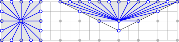
Figure 17. Maximal degenerations of K3 surfaces for $(18,2,0)_{1}$ and $(18,0,0)_{1}$ cusps of $F_{(2,2,0)}$

For the $(18,2,0)_{1}$-cusp, the maximal degeneration is a union of $16$ surfaces of $A_{0}^{-}$ type, which is ${\mathbb{P}}^{2}$ with a del Pezzo involution such that the quotient is the quadratic cone ${\mathbb{P}}(1,1,2)$. We may symbolically write it as $(A_{0}^{-}\raise 0.65pt\hbox{$\kern-2.0pt\phantom{.}^{-}$}\kern-4.0ptA_{0})^{8}$. This degeneration corresponds to the empty subdiagram of $G_{r}(18,2,0)$.

For an elliptic subdiagram $G\subset G_{r}(18,2,0)$, each relevant component (i.e. not lying entirely in the interior of the square) gives an ADE surface. Then the corresponding KSBA degeneration is their union glued along double curves. The ADE surfaces are obtained by smoothing some of the double curves in the maximal degeneration; these edges correspond to the vertices in $G$. All of the degenerations are of the “pumpkin type”, see [AE22, Fig. 2].

There is however a caveat: the $C_{3}$ diagram in the third row of Figure 19 should be treated instead as an $\kern-2.0pt\phantom{.}^{\prime}\kern-2.0pt\kern-1.0ptA_{3}^{\prime}$ diagram. This is because the diagrams $G$ are supposed to be subdiagrams of $G_{2}$, for the reflection group generated by the $(-2)$-roots, and $G_{r}$ is the Coxeter diagram for the full reflection group, which includes both $(-2)$ and $(-4)$-roots. There is a simple dictionary to translate from one to another, see [AE22, Fig. 15].

At the $(18,0,0)_{1}$-cusp, the degenerations are of the “smashed pumpkin type”, as in [AE22, Fig. 2]. It can be understood in the following way. Begin with a union of $18$ surfaces of $A_{0}^{-}$ type, $\cup_{i}^{18}(V_{i},D_{i})$, where $V_{i}\simeq{\mathbb{P}}^{2}$ with an involution $(x,y,z)\to(x,y,-z)$. The ramification divisor on $V_{i}$ is a line, and the boundary curves $D_{1}$, $D_{2}$ are a line and a conic. Consider two neighboring $V_{i}$, $V_{i+1}$ that are glued along a line $D_{1}$, so that $R\cap D_{1}=p$ is a point. Blow up this point in each of the surfaces to get $V^{\prime}_{i}$ and $V^{\prime}_{i+1}$, both isomorphic to ${\mathbb{F}}_{1}$. The strict preimage of $R^{\prime}\cap V^{\prime}_{i}$ is now a fiber $f$ of ${\mathbb{F}}_{1}$, and same for $V^{\prime}_{i+1}$. Contract by the linear system $|f|$. Then $V_{i}\cup V_{i+1}$ collapses to ${\mathbb{P}}^{1}\cup{\mathbb{P}}^{1}$ and the entire surface $\cup_{i=1}^{18}V_{i}$ which previously was represented by a “pumpkin” is partially collapsed, with the north and south poles colliding.

For the non-maximal degenerations we begin with a Coxeter diagram $G_{r}(19,1,1)$ as in [AET23, Fig. 4.1]. An elliptic subdiagram $G$ of this Coxeter diagram, as in the case above, corresponds to a union of ADE surfaces. We then perform the move described above to partially collapse it. The edge between $V_{i}$ and $V_{i+1}$ is always contracted, bringing the north and south poles of the pumpkin together. The components $V_{i}$ and $V_{i+1}$ are collapsed only if they are of the $A_{0}^{-}$ type, i.e. the conic $D_{2}$ in ${\mathbb{P}}^{2}$ was not smoothed out.

7.2. Type II stable models of K3 surfaces

The stable models in this case are very similar to the Type III models described above. They correspond to maximal parabolic subdiagrams $G\subset G_{r}$. After throwing away irrelevant connected components of $G$, each of the remaining components is a ${\widetilde{A}}{\widetilde{D}}{\widetilde{E}}$ subdiagram, giving an ${\widetilde{A}}{\widetilde{D}}{\widetilde{E}}$ surface.

7.3. Type III stable models of Enriques surfaces

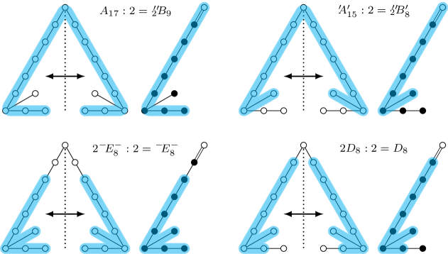
Figure 18. Max connected elliptic diagrams for $0$-cusp 2

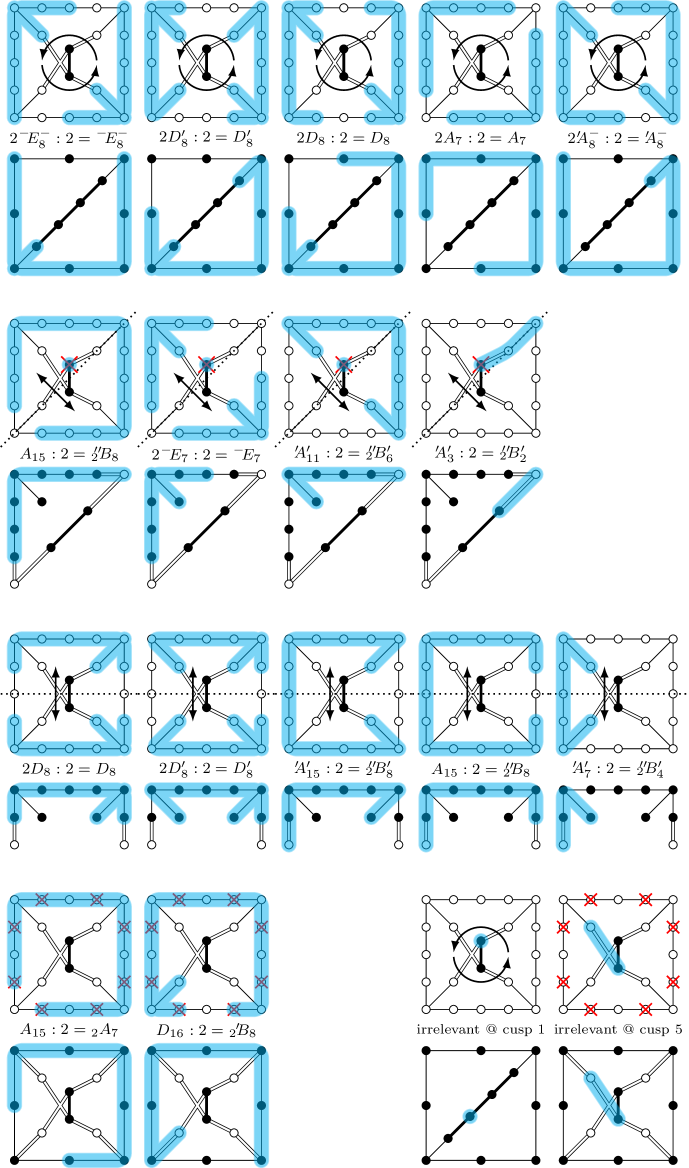
Figure 19. Max connected elliptic diagrams for $0$-cusps 1, 3, 4, 5

By Corollary 4.9 and the proof of Theorem 5.9, the description of the KSBA stable limit of Enriques pairs $(Z,\epsilon R_{Z})$ are now straightforward: these are simply quotients of KSBA stable limits of K3 pairs $(X,\epsilon R)$ by an Enriques involution. The latter acts in different ways, depending on the $0$-cusp of $F_{\rm En,2}$. The action is determined by the folding of the Coxeter diagram, as in Figures 7 and 8. Let us spell them out, representing the surface $(X,\epsilon R)$ by a sphere $S^{2}$.

(1) At the cusp 1, the action on $S^{2}$ is antipodal, with the quotient ${\mathbb{R}}{\mathbb{P}}^{2}$. So all irreducible components of $X=\cup V_{i}$ are interchanged in pairs $V_{i}\simeq V_{\sigma(i)}$. Then the normalization of $V_{i}\cup V_{\sigma(i)}/\iota_{{\rm En}}$ is isomorphic to the normalization of $V_{i}$.

(2, 3, 4) At these cusps the action on $S^{2}$ is a reflection which is different from the equatorial reflection defined by $\iota_{{\rm dP}}$. Some of the components $V_{i}$ of $X$ come in pairs, and some are fixed by $\iota_{{\rm En}}$. The latter ones are the $B_{n}$ surfaces of Section 6.6.

(5) Here the action of $\iota_{{\rm En}}$ on $S^{2}$ is the same as the action of $\iota_{{\rm dP}}$. Each component $V_{i}$ is fixed by $\iota_{{\rm En}}$ and the quotients are the surfaces described in Section 6.5.

In Figures 18 and 19 we list the maximal connected elliptic subdiagrams in the Coxeter diagrams, for each of the five $0$-cusps of $F_{\rm En,2}$. These then describe the largest possible irreducible components in $X$ and $Z=X/\iota_{{\rm En}}$. All other irreducible components correspond to the subdiagrams of these maximal ones, which are preserved by the folding symmetry.

The surfaces are glued according to the Coxeter diagram.

Example 7.1.

Consider the first surface $2\raise 0.65pt\hbox{$\kern-2.0pt\phantom{.}^{-}$}\kern-2.0ptE^{-}_{8}:2=\raise 0.65pt\hbox{$\kern-2.0pt\phantom{.}^{-}$}\kern-2.0ptE^{-}_{8}$ in Figure 19. The degenerate Enriques surface is irreducible and its normalization is an ADE surface of type $\raise 0.65pt\hbox{$\kern-2.0pt\phantom{.}^{-}$}\kern-2.0ptE_{8}^{-}$. It is then glued to itself by an isomorphism $D_{1}\to D_{2}$ between the two sides.

The Coxeter diagrams in Figures 7 and 8 also describe the ramification divisor $R_{Z}$ on the Type III degenerations $Z$. The boundary of each Coxeter diagram for the Cusps 1, 2, 3, 4, 5, i.e. the image of the boundary of the square or the triangle, represents the ramification divisor $R_{Z}$. Thus, in Cusps 1 and 5, $R_{Z}$ is a cycle, and in the other three cusps it is a chain.

7.4. Type II stable models of Enriques surfaces

Similarly, the irreducible components of Type II degenerations are described by the relevant components of the maximal parabolic subdiagrams in the Coxeter diagrams. We listed them in Figures 9 and 10. The folded Type II surfaces are described in Sections 6.5 (cusp 5) and 6.6 (cusps 2, 3, 4).

References

- [ABE22] Valery Alexeev, Adrian Brunyate, and Philip Engel, Compactifications of moduli of elliptic K3 surfaces: Stable pair and toroidal, Geom. Topol. 26 (2022), no. 8, 3525–3588.
- [AE22] Valery Alexeev and Philip Engel, Compactifications of moduli spaces of K3 surfaces with a nonsymplectic involution, arXiv:2208.10383 (2022).
- [AE23] by same author, Compact moduli of K3 surfaces, Ann. of Math. (2) 198 (2023), no. 2, 727–789.
- [AEH21] Valery Alexeev, Philip Engel, and Changho Han, Complete moduli of K3 surfaces with a nonsymplectic automorphism, Trans. Amer. Math. Soc., to appear (2021), arXiv:2110.13834.
- [AET23] Valery Alexeev, Philip Engel, and Alan Thompson, Stable pair compactification of moduli of K3 surfaces of degree 2, J. Reine Angew. Math. 799 (2023), 1–56.
- [AT21] Valery Alexeev and Alan Thompson, ADE surfaces and their moduli, J. Algebraic Geometry 30 (2021), 331–405, arXiv:1712.07932.
- [BB66] W. L. Baily, Jr. and A. Borel, Compactification of arithmetic quotients of bounded symmetric domains, Ann. of Math. (2) 84 (1966), 442–528.
- [Bir23] Caucher Birkar, Geometry of polarised varieties, Publ. Math. Inst. Hautes Études Sci. 137 (2023), 47–105.
- [CD89] François R. Cossec and Igor V. Dolgachev, Enriques surfaces. I, Progress in Mathematics, vol. 76, Birkhäuser Boston, Inc., Boston, MA, 1989.
- [CDL24] François R. Cossec, Igor Dolgachev, and Christian Liedtke, Enriques surfaces I, Springer Nature, 2024.
- [Cos83] François R. Cossec, Projective models of Enriques surfaces, Math. Ann. 265 (1983), no. 3, 283–334.
- [Cox35] H. S. M. Coxeter, Wythoff’s Construction for Uniform Polytopes, Proc. London Math. Soc. (2) 38 (1935), 327–339.
- [dFKX17] Tommaso de Fernex, János Kollár, and Chenyang Xu, The dual complex of singularities, Higher dimensional algebraic geometry—in honour of Professor Yujiro Kawamata’s sixtieth birthday, Adv. Stud. Pure Math., vol. 74, Math. Soc. Japan, Tokyo, 2017, pp. 103–129.
- [EF21] Philip Engel and Robert Friedman, Smoothings and rational double point adjacencies for cusp singularities, J. Differential Geom. 118 (2021), no. 1, 23–100.
- [Eng18] Philip Engel, Looijenga’s conjecture via integral-affine geometry, J. Differential Geom. 109 (2018), no. 3, 467–495.
- [Enr06] Federigo Enriques, Sopra le superficie algebriche di bigenere uno, Mem. Soc. Ital. Sci. XIV (1906), no. 3a, 327–352.
- [Fri15] Robert Friedman, On the geometry of anticanonical pairs, Preprint (2015), arXiv:1502.02560.
- [FS86] Robert Friedman and Francesco Scattone, Type degenerations of surfaces, Invent. Math. 83 (1986), no. 1, 1–39.
- [GH16] V. Gritsenko and K. Hulek, Moduli of polarized Enriques surfaces, K3 surfaces and their moduli, Progr. Math., vol. 315, Birkhäuser/Springer, [Cham], 2016, pp. 55–72.
- [GHK15a] Mark Gross, Paul Hacking, and Sean Keel, Mirror symmetry for log Calabi-Yau surfaces I, Publ. Math. Inst. Hautes Études Sci. 122 (2015), 65–168.
- [GHK15b] by same author, Moduli of surfaces with an anti-canonical cycle, Compos. Math. 151 (2015), no. 2, 265–291.
- [Hor78a] Eiji Horikawa, On the periods of Enriques surfaces. I, Math. Ann. 234 (1978), no. 1, 73–88.
- [Hor78b] by same author, On the periods of Enriques surfaces. II, Math. Ann. 235 (1978), no. 3, 217–246.
- [KK72] Peter Kiernan and Shoshichi Kobayashi, Satake compactification and extension of holomorphic mappings, Invent. Math. 16 (1972), 237–248.
- [KLSV18] János Kollár, Radu Laza, Giulia Saccà, and Claire Voisin, Remarks on degenerations of hyper-Kähler manifolds, Ann. Inst. Fourier (Grenoble) 68 (2018), no. 7, 2837–2882.
- [KM98] János Kollár and Shigefumi Mori, Birational geometry of algebraic varieties, Cambridge Tracts in Mathematics, vol. 134, Cambridge University Press, Cambridge, 1998, With the collaboration of C. H. Clemens and A. Corti, Translated from the 1998 Japanese original.
- [Kol23] János Kollár, Families of varieties of general type, Cambridge Tracts in Mathematics, vol. 231, Cambridge University Press, Cambridge, 2023.
- [Kul77] Vik. S. Kulikov, Degenerations of surfaces and Enriques surfaces, Izv. Akad. Nauk SSSR Ser. Mat. 41 (1977), no. 5, 1008–1042, 1199.
- [KX20] János Kollár and Chen Yang Xu, Moduli of polarized Calabi-Yau pairs, Acta Math. Sin. (Engl. Ser.) 36 (2020), no. 6, 631–637.
- [Laz16] Radu Laza, The KSBA compactification for the moduli space of degree two pairs, J. Eur. Math. Soc. (JEMS) 18 (2016), no. 2, 225–279.
- [LO21] Radu Laza and Kieran O’Grady, GIT versus Baily-Borel compactification for ’s which are double covers of , Adv. Math. 383 (2021), Paper No. 107680, 63.
- [Loo76] Eduard Looijenga, Root systems and elliptic curves, Inventiones mathematicae 38 (1976), no. 1, 17–32.
- [Loo78] by same author, On the semi-universal deformation of a simple-elliptic hypersurface singularity. II. The discriminant, Topology 17 (1978), no. 1, 23–40.
- [Loo86] by same author, New compactifications of locally symmetric varieties, Proceedings of the 1984 Vancouver conference in algebraic geometry, CMS Conf. Proc., vol. 6, Amer. Math. Soc., Providence, RI, 1986, pp. 341–364.
- [Loo03] by same author, Compactifications defined by arrangements. II. Locally symmetric varieties of type IV, Duke Math. J. 119 (2003), no. 3, 527–588.
- [Mor81] David R. Morrison, Semistable degenerations of Enriques’ and hyperelliptic surfaces, Duke Math. J. 48 (1981), no. 1, 197–249.
- [Nam85] Yukihiko Namikawa, Periods of Enriques surfaces, Math. Ann. 270 (1985), no. 2, 201–222.
- [Nik79] V. V. Nikulin, Integer symmetric bilinear forms and some of their geometric applications, Izv. Akad. Nauk SSSR Ser. Mat. 43 (1979), no. 1, 111–177, 238.
- [Pin77] H. C. Pinkham, Simple elliptic singularities, Del Pezzo surfaces and Cremona transformations, Several complex variables (Proc. Sympos. Pure Math., Vol. XXX, Part 1, Williams Coll., Williamstown, Mass., 1975), Proc. Sympos. Pure Math., vol. Vol. XXX, Part 1, Amer. Math. Soc., Providence, RI, 1977, pp. 69–71.
- [PP81] Ulf Persson and Henry Pinkham, Degeneration of surfaces with trivial canonical bundle, Ann. of Math. (2) 113 (1981), no. 1, 45–66.
- [PS20] Chris Peters and Hans Sterk, On K3 double planes covering Enriques surfaces, Math. Ann. 376 (2020), no. 3-4, 1599–1628.
- [Sha81] Jayant Shah, Degenerations of surfaces of degree , Trans. Amer. Math. Soc. 263 (1981), no. 2, 271–308.
- [Ste91] Hans Sterk, Compactifications of the period space of Enriques surfaces. I, Math. Z. 207 (1991), no. 1, 1–36.
- [Sym03] Margaret Symington, Four dimensions from two in symplectic topology, Topology and geometry of manifolds (Athens, GA, 2001), Proc. Sympos. Pure Math., vol. 71, Amer. Math. Soc., Providence, RI, 2003, pp. 153–208.
- [Vin72] È. B. Vinberg, The groups of units of certain quadratic forms, Mat. Sb. (N.S.) 87(129) (1972), 18–36.
- [Vin75] by same author, Some arithmetical discrete groups in Lobačevskiĭ spaces, Discrete subgroups of Lie groups and applications to moduli (Internat. Colloq., Bombay, 1973), Oxford Univ. Press, Bombay, 1975, pp. 323–348.