Training Neural Networks on RAW and HDR Images for Restoration Tasks

Abstract

The vast majority of standard image and video content available online is represented in display-encoded color spaces, in which pixel values are conveniently scaled to a limited range (0–1) and the color distribution is approximately perceptually uniform. In contrast, both camera RAW and high dynamic range (HDR) images are often represented in linear color spaces, in which color values are linearly related to colorimetric quantities of light. While training on commonly available display-encoded images is a well-established practice, there is no consensus on how neural networks should be trained for tasks on RAW and HDR images in linear color spaces. In this work, we test several approaches on three popular image restoration applications: denoising, deblurring, and single-image super-resolution. We examine whether HDR/RAW images need to be display-encoded using popular transfer functions (PQ, PU21, mu-law), or whether it is better to train in linear color spaces, but use loss functions that correct for perceptual non-uniformity. Our results indicate that neural networks train significantly better on HDR and RAW images represented in display-encoded color spaces, which offer better perceptual uniformity than linear spaces. This small change to the training strategy can bring a very substantial gain in performance, up to 10–15 dB.

1 Introduction

Neural networks are typically trained on images represented in display-encoded color spaces, such as BT.709 with the sRGB non-linearity [2]. These are known as display-encoded color spaces because they are commonly used to drive displays. HDR images, as well as RAW images containing camera sensor values, are often represented in linear color spaces, in which the pixel values are proportional to colorimetric or photometric light quantities. Notably, linear color spaces are very far from being perceptually uniform [16]: the same change in physical units is much less visible at high brightness than low. Modern perceptual uniform transfer functions, such as the SMPTE PQ (perceptual quantizer) [19] and PU21 (perceptually uniform transform) [17] have been developed to address this. By way of example, according to the PQ function, a change of 1 cd/m² starting from near darkness (0.005 cd/m²) is over 150 times more visible than the same change starting at 100 cd/m².

There are arguments both for and against training neural networks with images in linear spaces. If a plain L1 or L2 loss is used to train networks for linear data, we run the risk that the network will overfit for bright colors, and introduce unacceptable inaccuracies for darker colors. Additionally, if we wish to avoid visible quantization errors, pixel values in linear color spaces must be represented with more bits than display-encoded spaces. However, any physical phenomena involving light, such as lens blur, motion blur, or noise, can only be modeled in a physically plausible manner in linear color spaces. Therefore, physically plausible image formation models for blur, noise and sampling must be defined in linear color spaces, and by analogy, the inverse problems of deblurring, denoising and super-resolution should also be formulated in linear color spaces. It is unknown, however, whether neural networks can benefit from the physical properties of linear color spaces.

In this work, we want to determine what training strategy leads to the best results. Should we train neural networks in display-encoded or linear color spaces (Section 3)? If we train networks in linear color spaces, should we use a loss function that compensates for perceptual non-uniformity (Section 3.2)? There is no consensus in the literature on these questions. Many works train on images in linear color spaces and use an L1 loss [26, 6]. Some use a loss with perceptual encoding [7, 11, 18]. Our goal is to find empirical evidence to motivate a training strategy for image restoration techniques trained on HDR/RAW images. To that end, we collect a dataset of HDR images and train six networks to perform common image restoration tasks: single-image super-resolution, denoising, and deblurring (Section 4).

Rather than proposing a new method, this paper is a benchmark and reproduction study intended to settle these open questions. Our results serve as best practice guidelines for future ML methods operating on HDR and RAW content. Our results (Section 5) show a clear benefit in training networks in display-encoded color spaces, offering a gain in performance up to 10–15 dB for these applications.

2 Related work

2.1 Imaging RAW pixels

RAW image data, captured directly from image sensors, preserves unprocessed and uncompressed pixel information, thereby providing rich information for restoration techniques. RAW image formats also represent pixels in linear color spaces, which facilitate physically plausible modeling of camera noise [1]. Early works [9, 10] in this area mainly focused on noise reduction and artifact suppression based on statistical models of noise. With the advent of deep learning, restoration in the RAW domain has witnessed a paradigm shift. [24, 4, 20] pioneered by the integration of deep neural networks for denoising. Those early works, however, targeted sRGB images, typically with synthetic additive Gaussian noise. Since denoising is likely to be integrated in the very early stages of the ISP pipeline, it should operate on linear RAW pixel values instead.

Surprisingly, many deep-learning methods proposed for processing RAW images were never tested on RAW images [25, 15]. Instead, they opted to work with display-encoded images in the sRGB space, and assumed additive Gaussian noise. Both assumptions make input data very different from RAW sensor pixel values, raising the question on whether these methods would be equally effective for real camera data. Other methods that were trained and tested on RAW images [26, 6], did so directly on linear color values and used an L1 loss. Our work demonstrates this strategy often fails to achieve good results.

2.2 High Dynamic Range (HDR) imaging

The dynamic range is the contrast between the brightest and darkest parts of an image or video. Notably, the dynamic range the human eye can see is extremely high and much larger than what most standard dynamic range (SDR) capture and display pipelines are capable of [13]. High Dynamic Range (HDR) is a term for a range of technologies that enhance the visual quality and realism of content by providing a wider than normal dynamic range [21].

A key problem in HDR imaging involves merging multiple exposures into an HDR image while reducing “ghosting” artifacts due to motion [11]. Another problem is tone-mapping of HDR scenes to the dynamic range that can be shown on a display [21]. Yet another is the reconstruction of an HDR image from a single exposure (i.e. inverse-tone mapping) [7, 12]. However, standard reconstruction problems like denoising, single-image super-resolution, or deconvolution/deblurring, are also relevant for HDR imaging.

This work focuses on how HDR data in linear color spaces was handled in these previous works. Both Eilertsen et al. [7] and Kalantari et al. [11] trained the networks to directly predict HDR images in a linear color space. However, to compensate for the perceptual non-uniformity of that space, Eilertsen et al. used the logarithmic function, and Kalantari et al. introduced the $\mu$-law (explained in detail in Section 3). Mildenhall et al. [18] used a relative loss, similar to SMAPE (explained in Section 3.2), to train a NeRF on RAW images. The networks intended to reconstruct HDR UHD video content [12] were directly trained to predict display-encoded frames using the PQ OETF [19].

3 Representations

3.1 Pixel encodings

In this work, we explore popular perceptual pixel value representations from the literature for use in machine learning applications. The main question that arises is what representation – linear or display encoded – is most suitable for deep-learning networks. The linear representation should be better to model physical phenomena (assuming neural networks are able to take advantage of this benefit). However, the display-encoded representations are more data-efficient (requiring fewer bits) and have better perceptual uniformity. Moreover, most existing methods have been trained on display-encoded representations, as these are commonly used for SDR content widely available online. To answer the question above, we tested four representations: one linear and three display-encoded:

Linear:

linear RGB pixel values with BT.709 primaries, scaled between 0 and 1;

$\mu$-law:

a transfer function commonly used for perceptual audio encoding. Kalantari et al. [11] proposed to encode HDR images using the $\mu$-law function:

$$v_{\mu}(l)=\frac{\log(1+\mu\,l)}{\log(1+\mu)}$$ (1)

with the constant $\mu=5000$. $l$ is a relative linear (RGB) color value scaled to the range 0–1.

PQ (perceptual quantizer):

display-encoding for HDR content [19], used in video coding and display standards. The PQ encoding was applied separately to each RGB channel. Input linear values were given in absolute units and scaled to the range 0.005 to 10 000 (see Section 4.2).

PU21 (perceptually uniform transform):

a transform similar to PQ but based on more modern data. It was originally proposed as an encoding of HDR images to be used with existing “standard” dynamic range metrics [17, 3]. For the PU21 encoding we use the quadratic function fitted to the original curve (which was derived numerically)

$$v_{\text{PU21}}(L)=a\,(\log_{2}(L)-L_{\text{min}})^{2}+b\,(\log_{2}(L)-L_{\text{min}})\,,$$ (2)

where $L$ is an absolute linear (RGB) color value (in the range 0.005–10 000) and the fitted parameters are $a=0.001908$, $b=0.0078$ and $L_{\text{min}}=\log_{2}(0.005)$. The encoded values are between 0 and 1. The inverse is given by:

$$v^{-1}_{\text{PU21}}(V)=2^{\frac{2\,a\,L_{\text{min}}-b+\sqrt{b^{2}+4\,a\,V}}{2\,a}}\,.$$ (3)

The functions above were fitted to the PU21 encoding for a banding model without the influence of glare (details in [17]) and are more computationally efficient than the PQ encoding or the original source code for PU21. This encoding was applied to each linear RGB channel in the same manner as PQ (see Section 4.2).

The pixel encodings described above are plotted in Figure 1. It can be observed that both PQ and PU21 share very similar shapes, but PQ does not reach 0 for the minimum encoded value (0.005). The $mu$-law has a much shallower shape for values below 1, which means these values are encoded with less precision. Finally, linear encoding over-emphasizes large pixel values.

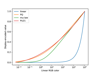
Figure 1: Perceptual encoding functions used to transform linear RGB color values to an approximately perceptually uniform space. A logarithmic scale is used for the x-axis to account for Weber’s law. Following BT.2100, the range of interest for encoded values is between 0.005 and 10 000. Note, however, that in our experiments, we used a smaller range between 0 and 4 000. Since $\mu$-law encoding expects input values between 0 and 1, the values were divided by 10 000 before passing to the function in Eq. (1).

3.2 Loss functions

In addition to the way pixels are encoded, the loss function is a key feature of training neural networks. Most image restoration problems can be effectively trained using L1 or L2 norms on pixel values as a loss function. However, this is not necessarily true when pixel values are represented in linear color spaces (e.g. RAW or HDR images), as they are perceptually nonuniform — a small error at low brightness is more visible than the same error at large brightness levels. This problem can be avoided by first converting the pixel values we mean to compare to a color space that is more perceptually uniform, so that the loss function becomes

$$\ell=||p(f_{\bm{\phi}}(\bm{x}))-p(\bm{y})||_{1}$$ (4)

where $f_{\bm{\phi}}(\cdot)$ is a network with the weights $\bm{\phi}$, $\bm{x}$ is input, $\bm{y}$ is a reference (label) and the $p(\cdot)$ is a perceptual encoding function such as $\mu$-law, PQ or PU21 (all introduced in Section 3). One important consideration is that the values passed to the function $p(\cdot)$ must be within the allowed range (e.g. greater than 0.005 for PQ and PU21). This means that out-of-range values must be clamped. Both PQ and PU21 require absolute photometric values, which correspond to light emitted from a display (e.g. between 0.005 and 10 000).

Another perceptual uniformity strategy is using the symmetric mean absolute percentage error (SMAPE) as a loss:

$$\ell=\left\lVert\frac{|f_{\bm{\phi}}(\bm{x})-\bm{y}|}{|f_{\bm{\phi}}(\bm{x})|+|\bm{y}|+\epsilon}\right\rVert_{1}\,,$$ (5)

where $\epsilon$ is a small constant avoiding division by 0. Dividing by the sum of absolute values makes the error relative and more perceptually uniform, following Weber’s law.

4 Experiments

In this work, we focus on image restoration problems (denoising, deblurring, and single-image super-resolution), which aim to generate a higher-quality version of the input image. We exclude higher-level tasks (e.g. recognition) as they involve very different losses to those used for restoration. We also do not consider the tasks in which input and output images differ in dynamic range — tone mapping and single-image HDR reconstruction, as these tasks would only allow us to test either the representations (for tone mapping) or the loss functions (single-image HDR reconstruction) but not both at once.

To compare the effectiveness of different loss functions and pixel encodings, we train networks with HDR images on three tasks: image denoising, deblurring, and super-resolution. For each task, we choose two different neural networks: one a traditional technique and the second a more recent method. We follow the training settings proposed in the original works. EDSR (2017) [14] and Real-ESRGAN (2021) [23] are used for the task of image super-resolution (4x). The downsampled images used for training were created using a bilinear filter. For image deblurring, we train GFNNet (2018) [29] and MirNet-v2 (2022) [27]. The networks are trained on images affected by Gaussian blur with sigma values of 8 in both directions. DnCNN (2017) [28] and SADNet (2020) [5] are used for denoising of HDR images. Physically plausible simulated camera noise (photon and readout noise) was added to the training images [9].

All networks are trained using the code provided by the authors on their GitHub repositories. We adopted the same training schemes as the original papers to train each network, including the optimizer and learning rate. We trained each network for a different number of epochs to ensure that convergence was reached. EDSR was trained for 3k epochs, 1.5k epochs for Real-ESRGAN, 1k epochs for MirNet-v2, GFNNet, DnCNN, and SADNet.

4.1 Datasets

We used 106 HDR images from the HDR Photographic Survey [8], as well as HDR videos from the SJTU HDR Video Sequences [22]. As frames originating from the same video share similarities, we used one demo HDR frame provided for each video, adding an additional 16 reference images to the dataset. 60% of images were selected for training, 20% for validation, and the remaining 20% were used for testing. To verify the networks’ generalization ability to exposure variations, the testing data set was augmented five-fold by multiplying it with a random exposure coefficient drawn from a uniform distribution between 0.1 and 0.9. We did not directly use RAW images in our experiments because they tend to contain more noise than their HDR counterparts (merging multiple exposures can radically reduce noise). However, the simulated noise used for denoising and the exposure augmentation technique made the prepared HDR images very close to demosaiced RAW images.

4.2 HDR/RAW training cases

Table 1: The 8 combinations of pixel encoding and loss functions tested in our experiments.

Label	Pixel encoding	Loss function
Linear-L1	Linear	L1
PQ-L1	PQ	L1
PU21-L1	PU21	L1
$\mu$-L1	$\mu$-law (mu-law)	L1
Linear-PQ	Linear	PQ
Linear-PU21	Linear	PU21
Linear-$\mu$	Linear	$\mu$-law (mu-law)
Linear-smape	Linear	SMAPE

We tested 8 combinations of pixel encodings and loss functions, listed in Table 1. All perceptual pixel encodings (PQ, PU21 and $\mu$-law, see Section 3) were used with a regular L1 loss as the encoded values are expected to be approximately perceptually uniform and so should not require a custom loss function. However, when no encoding was used (labeled as linear), we used either an L1 loss or one of the losses described in Section 3.2. We also experimented with losses that were a sum of two terms, such as L1 and PQ-encoded L1, but they performed no better than individual loss terms. Figure 2 shows a diagram of our training setup.

Since PQ and PU21 both require pixel values in absolute units (of light, as emitted by a display), the linear pixel values were scaled to the range 0.005–4 000. Although both encodings allow values up to 10 000 (nit), 4 000 was selected as being more representative of realistic peak luminance values for a high-quality HDR display. For other pixel encodings, the linear color values were scaled in the 0–1 range. By following these steps, we ensure all values passed to the networks (for every encoding) were between 0 and 1, as is typical for training.

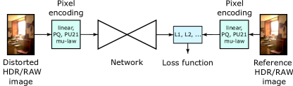
Figure 2: Training on HDR/RAW images. Training pairs were first (optionally) encoded from a linear to a perceptually uniform color space using PQ, PU21 or a $\mu$-law transfer function (explained in Section 3). If no pixel encoding was applied (linear), one of the loss functions from Section 3.2 was used to account for the perceptual non-uniformity.

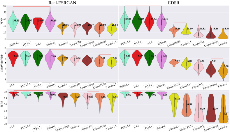
Figure 3: Single-image super-resolution results for the two networks (columns) and three metrics (rows). The violin shape represents the distribution across the testing set. A thin black line shows the range of quality scores (excluding outliers), and the thicker line shows the region between the 25th and 75th percentiles. The dot and numerical value represent the median. Red horizontal lines above the violin plots denote the groups of conditions for which we have no evidence of statistically significant differences. Results are sorted from the best on the left to the worst on the right. The colors are different for each combination of representation and loss and are consistent across plots.

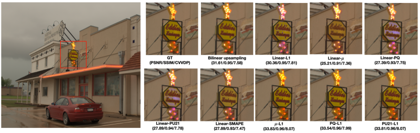
Figure 4: Example results for single-image super-resolution with EDSR [14]. The numbers in parentheses show PSNR, SSIM, and ColorVideoVDP quality values (the higher, the better) for the reconstructed image.

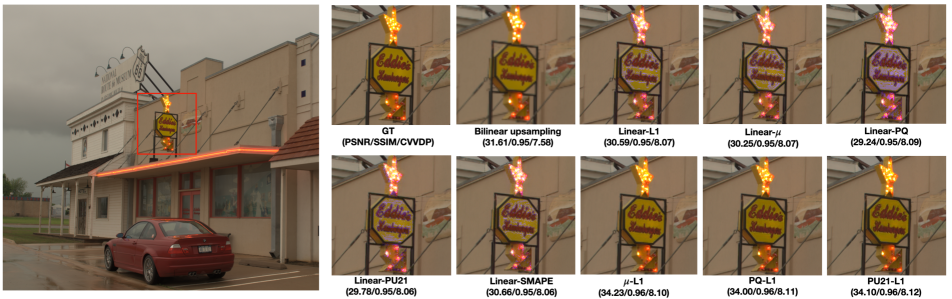
Figure 5: Example results for single-image super-resolution with Real-ESRGAN [23].

5 Results

To evaluate the results (see Table 2), we used three image quality metrics: PSNR, SSIM and ColorVideoVDP. PSNR and SSIM were selected as the two most widely used metrics. ColorVideoVDP was selected because it natively supports HDR images and was designed to compare color images and videos. To adapt PSNR and SSIM to HDR images, we used the PU21 encoding [17], i.e. PSNR was computed on the PU21-encoded RGB pixels. SSIM was computed on the luma channel of the PU21-encoded pixels.

5.1 Single-image super-resolution

The numerical results for the two single-image super-resolution methods can be found in the top row of Table 2, in Figure 3, and examples of visual results in Figure 4 and Figure 5. In Figure 3 we visualize the distribution of the quality scores across the entire test set and also report the results of pair-wise t-tests (two-tailed, $\alpha=0.05$, $N=144$). The violin plots are sorted left-to-right from the best-performing condition to the worst. Red horizontal lines connecting two or more violin plots signify no evidence of statistically significant differences within that group. Conversely, conditions that are not joined by a common line were found to have performances that differ at a statistically significant level.

The results in Figure 3 indicate a substantial gain in performance of both super-resolution methods (10–15 dB, as compared to Linear-L1) when one of the perceptual pixel representations is used. However, we have no statistical evidence showing that one perceptual representation is better than the others. Most perceptual loss functions improve the results of Real-ESRGAN as compared to plain L1 (1–3 dB), but they also make the results worse for ESDR. The visual results in Figure 4 and Figure 5 demonstrate that all trained networks can produce sharp images (as compared to bilinear upsampling), but some result in incorrect colors, in particular in bright areas. The networks that used perceptual pixel encodings do not suffer from these color artifacts.

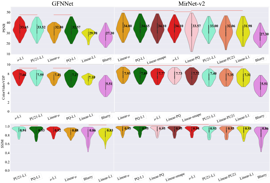
Figure 6: Deblurring results for the two networks (columns) and three metrics (rows). A few configurations are missing for GFNet as network training failed to converge for those. The notation is the same as in Figure 3.

5.2 Deblurring

Deblurring results are different for the two tested methods and will be discussed separately. GFNNet failed to train and converge for several of the tested loss functions; it did, however, converge for all perceptual pixel encodings. As shown in Figure 6 and Table 2, the best performance was obtained using either the $\mu$-law or PU21 pixel encodings, resulting in an improvement of about 3.8 dB compared to the plain Linear-L1 configuration. The improvement was smaller (but still significant) for the PQ pixel encoding and linear encoding using the $\mu$-law loss function. Visually (see supplementary, Figure 10) the Linear-L1 configuration resulted in artifacts in the form of vertical stripes. These artifacts were also present but less noticeable for other configurations. The PQ-L1 format resulted in a slightly softer image.

Deblurring with MirNet-v2 produced better results than for GFNNet. Similarly as for GFNNet, the worst results were achieved by the plain linear-L1 configuration. The best results were obtained by a linear encoding with the $\mu$-law loss, PQ and $\mu$-law pixel encodings (gain of 2–3 dB). Interestingly, the PU21 pixel encoding resulted in worse results (see supplementary Figure 10, note the visual results’ softer appearance), though the reason is unclear.

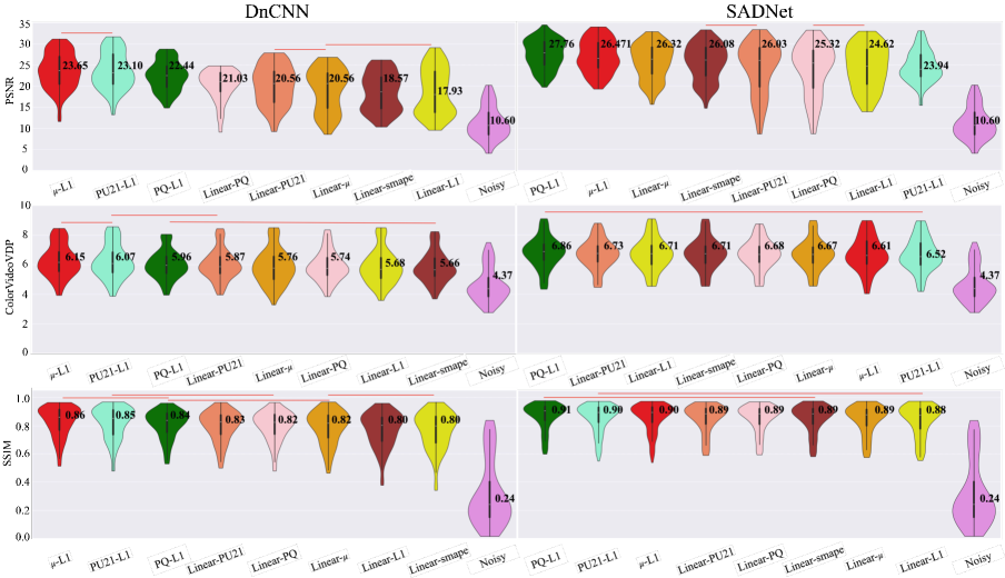
Figure 7: Denoising results for the two networks (columns) and three metrics (rows) The notation is the same as in Figure 3.

			PU21-L1	PQ-L1	$\mu$-L1	Linear-L1	Linear-PU21	Linear-PQ	Linear-$\mu$	Linear-SMAPE	Naive
Super-resolution	EDSR	SSIM	0.96	0.96	0.96	0.74	0.51	0.39	0.27	0.39	0.95
		PSNR	35.91	35.86	35.74	21.09	23.576	16.82	14.34	15.16	34.18
		CVVDP	8.40	8.37	8.38	6.89	7.22	6.34	5.58	5.81	7.99
	Real-ESRGAN	SSIM	0.95	0.95	0.96	0.84	0.86	0.86	0.87	0.88	0.95
		PSNR	35.45	35.37	34.97	25.55	26.80	28.94	28.96	28.28	34.18
		CVVDP	8.33	8.33	8.38	7.29	7.44	7.82	7.92	7.57	7.99
Deblurring	GFNNet	SSIM	0.94	0.93	0.92	0.83	N/A	N/A	0.88	N/A	0.87
		PSNR	33.52	32.57	33.65	29.98	N/A	N/A	32.80	N/A	27.30
		CVVDP	7.59	7.27	7.66	7.09	N/A	N/A	7.41	N/A	5.51
	MirNet-v2	SSIM	0.93	0.95	0.94	0.93	0.93	0.95	0.95	0.95	0.87
		PSNR	32.99	34.65	34.10	31.98	32.06	33.57	34.80	34.10	27.30
		CVVDP	7.40	7.89	7.77	7.31	7.35	7.73	7.93	7.72	5.51
Denoising	DnCNN	SSIM	0.85	0.84	0.86	0.80	0.83	0.83	0.82	0.80	0.24
		PSNR	23.10	22.44	23.65	17.93	20.56	21.03	20.56	18.57	10.60
		CVVDP	6.07	5.96	6.15	5.68	5.87	5.74	5.76	5.66	4.37
	SADNet	SSIM	0.90	0.91	0.90	0.88	0.89	0.89	0.88	0.89	0.24
		PSNR	23.94	27.76	26.47	24.62	26.03	25.32	26.32	26.08	10.60
		CVVDP	6.52	6.86	6.61	6.71	6.73	6.68	6.67	6.71	4.37

Table 2: The median values for evaluation results. The last column ’Naive’ is bilinear-upsampling results for super-resolution experiments, original blurry images for deblurring experiments, and the original noisy images for denoising experiments. The best performing scores are annotated in red, while the second best one is in blue. The ”N/A” entries correspond to the cases for which the training failed.

5.3 Denoising

For denoising networks, PSNR had more distinctive and slightly different results than ColorVideoVDP and SSIM, as seen in Figure 7 and Table 2. We investigated this discrepancy further by comparing pairs of conditions for which the metric predictions differed the most. We observed that both denoising methods, in particular DnCNN, resulted in images that differed in brightness, tone, color, and contrast from the original. Even though such changes may be less perceptually objectionable (and difficult to notice without a reference), PSNR was very sensitive to them. Both ColorVideoVDP and SSIM put more emphasis on structural distortions and seemed to correlate better with perceived quality.

For both denoising methods, perceptual pixel encodings produced the best results in most cases. $\mu$-law and PU21 performed the best for DnCNN, followed by PQ, which performed slightly worse according to PSNR and ColorVideoVDP. In the case of SADNet, ColorVideoVDP could not distinguish between any of the configurations (no evidence of statistical differences). While $\mu$-law consistently produced the highest metric scores for SADNet, PU21 was the second best in terms of SSIM, but the last in terms of PSNR. We attribute this discrepancy to color shifts (SSIM is insensitive to color changes). The visual results (see supplementary, Figure 10) show changes in color for Linear-PQ and Linear-PU. As a result, these two configurations have lower PSNR than the input noisy image (but higher ColourVideoVDP index because of the denoising).

6 Conclusions

The results across six tested methods clearly indicate that networks for image restoration should be trained on HDR/RAW images that are encoded using one of the perceptual transforms: PU21, PQ, or $\mu$-law. We did not find sufficient evidence to recommend one transform over another across all applications. However, we observed slightly worse performance of PQ for GFNNet, and PU21 for MirNet-v2 and SADNet. $\mu$-law encoding was robust across different methods but did not always produce the best results. Both $\mu$-law and PU21 use simpler and more computationally efficient formulas. PQ fails to scale the resulting values to a 0–1 range (see Figure 1), which may cause practical issues. Unlike the $\mu$-law, PQ and PU21 were derived from psychophysical data and have stronger perceptual bases. As the differences in performance between the three transforms are mostly small, we recommend using any of them, as this offers a substantial gain in performance over not using them at all. The actual gain in performance is application-specific and can be as large as 10–15 dB as compared to the “default” approach of training linear color values with an L1 loss. Using linear color values in tandem with a loss function that employs perceptual encoding seems to be less effective across the tested applications.

The empirical findings in this work are relevant as they show that very small changes in training strategy (“one-liners”) can substantially improve the results of neural networks trained for popular tasks on HDR or RAW images. Moreover, the winning strategy of using perceptual pixel coding is rarely used in practice. More often, networks are trained in linear color spaces using an L1 cost function [26, 6], or at most, use a perceptual encoding loss [7, 11, 18] — both strategies shown in this work to under-perform. We hope our findings help practitioners in designing better training configurations for HDR/RAW images.

Supplementary Material

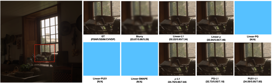
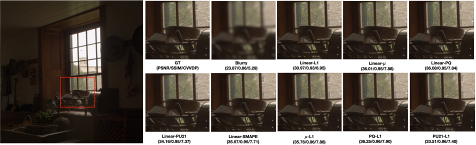
Figure 8: Example results for deblurring with GFNNet. The results are missing for Linear-PQ, Linear-PU21, and Linear-SMAPE, as the networks failed to converge for these configurations.

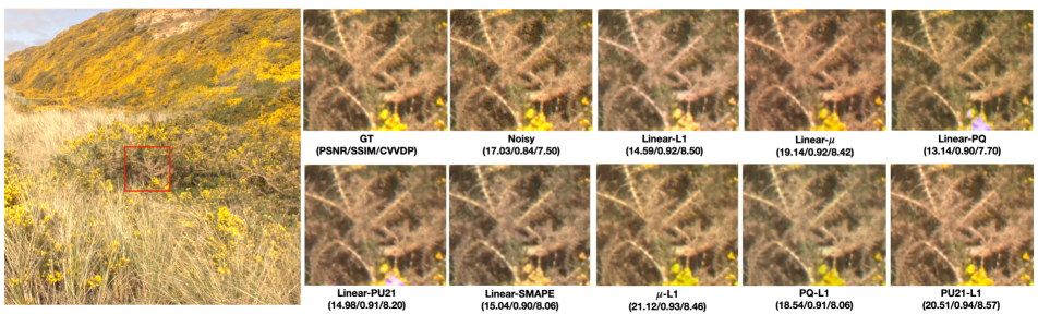
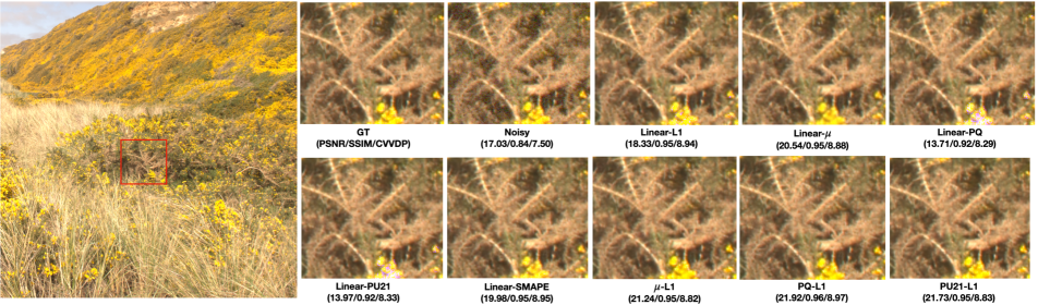
Figure 9: Example results for deblurring with MirNet-v2

Figure 10: Example results for denoising with DnCNN (top) and SADNet (bottom).

7 Visual results

This supplementary material contains additional visual results for the networks tested in our work.

• Deblurring, GFNNet - Figure 10

• Deblurring, MirNet-v2 - Figure 10

• Denoising, GFNNet - Figure 10, top

• Denoising, SADNet - Figure 10, bottom

References

- Aguerrebere et al. [2013] Cecilia Aguerrebere, Julie Delon, Yann Gousseau, and Pablo Musé. Study of the digital camera acquisition process and statistical modeling of the sensor raw data. 2013. hal-00733538.
- Anderson et al. [1996] Matthew Anderson, Ricardo Motta, Srinivasan Chandrasekar, and Michael Stokes. Proposal for a standard default color space for the internet - sRGB. In Color and Imaging Conference, pages 238–245. Society for Imaging Science and Technology, 1996.
- Aydın et al. [2008] Tunç O. Aydın, Rafal Mantiuk, and Hans-Peter Seidel. Extending quality metrics to full luminance range images. In Human Vision and Electronic Imaging, page 68060B. Spie, 2008.
- Burger et al. [2012] Harold C Burger, Christian J Schuler, and Stefan Harmeling. Image denoising: Can plain neural networks compete with BM3D? In CVPR, pages 2392–2399. IEEE, 2012.
- Chang et al. [2020] Meng Chang, Qi Li, Huajun Feng, and Zhihai Xu. Spatial-adaptive network for single image denoising. In Computer Vision – ECCV 2020, pages 171–187. Springer, 2020.
- Chen et al. [2018] Chen Chen, Qifeng Chen, Jia Xu, and Vladlen Koltun. Learning to see in the dark. In CVPR, page 3291–3300, Salt Lake City, UT, 2018. IEEE.
- Eilertsen et al. [2017] Gabriel Eilertsen, Joel Kronander, Gyorgy Denes, Rafał K. Mantiuk, and Jonas Unger. HDR image reconstruction from a single exposure using deep CNNs. ACM Transaction on Graphics, 36(6):Article 178, 2017.
- Fairchild [2007] Mark D. Fairchild. The HDR Photographic Survey. Color and Imaging Conference, 15(1):233–238, 2007.
- Foi et al. [2008] Alessandro Foi, Mejdi Trimeche, Vladimir Katkovnik, and Karen Egiazarian. Practical Poissonian-Gaussian noise modeling and fitting for single-image raw-data. IEEE Transactions on Image Processing, 17(10):1737–54, 2008.
- Hwang et al. [2011] Youngbae Hwang, Jun-Sik Kim, and In So Kweon. Difference-based image noise modeling using skellam distribution. IEEE Transactions on Pattern Analysis and Machine Intelligence, 34(7):1329–1341, 2011.
- Kalantari and Ramamoorthi [2017] Nima Khademi Kalantari and Ravi Ramamoorthi. Deep high dynamic range imaging of dynamic scenes. ACM Transactions on Graphics, 36(4):1–12, 2017.
- Kim et al. [2019] Soo Ye Kim, Jihyong Oh, and Munchurl Kim. Deep SR-ITM: Joint learning of super-resolution and inverse tone-mapping for 4k UHD HDR applications. In CVPR, pages 3116–3125, 2019.
- Kunkel and Reinhard [2010] Timo Kunkel and Erik Reinhard. A reassessment of the simultaneous dynamic range of the human visual system. In Proceedings of the 7th Symposium on Applied Perception in Graphics and Visualization, 2010.
- Lim et al. [2017] Bee Lim, Sanghyun Son, Heewon Kim, Seungjun Nah, and Kyoung Mu Lee. Enhanced deep residual networks for single image super-resolution. In CVPR workshops, pages 136–144, 2017.
- Liu et al. [2020] Lin Liu, Xu Jia, Jianzhuang Liu, and Qi Tian. Joint Demosaicing and Denoising With Self Guidance. In 2020 IEEE/CVF Conference on Computer Vision and Pattern Recognition (CVPR), pages 2237–2246. IEEE, 2020.
- Mantiuk et al. [2004] Rafal Mantiuk, Grzegorz Krawczyk, Karol Myszkowski, and Hans-Peter Seidel. Perception-motivated high dynamic range video encoding. ACM Transactions on Graphics (TOG), 23(3):733–741, 2004.
- Mantiuk and Azimi [2021] Rafal K. Mantiuk and Maryam Azimi. PU21: A novel perceptually uniform encoding for adapting existing quality metrics for HDR. In 2021 Picture Coding Symposium (PCS), pages 1–5. IEEE, 2021.
- Mildenhall et al. [2022] Ben Mildenhall, Peter Hedman, Ricardo Martin-Brualla, Pratul P. Srinivasan, and Jonathan T. Barron. NeRF in the Dark: High Dynamic Range View Synthesis from Noisy Raw Images. In 2022 IEEE/CVF Conference on Computer Vision and Pattern Recognition (CVPR), pages 16169–16178. IEEE, 2022.
- Miller et al. [2013] S. Miller, M. Nezamabadi, and S. Daly. Perceptual Signal Coding for More Efficient Usage of Bit Codes. SMPTE Motion Imaging Journal, 122(4):52–59, 2013.
- Nam et al. [2016] Seonghyeon Nam, Youngbae Hwang, Yasuyuki Matsushita, and Seon Joo Kim. A holistic approach to cross-channel image noise modeling and its application to image denoising. In Proceedings of the IEEE conference on computer vision and pattern recognition, pages 1683–1691, 2016.
- Reinhard et al. [2010] Erik Reinhard, Wolfgang Heidrich, Paul Debevec, Sumanta Pattanaik, Greg Ward, and Karol Myszkowski. High dynamic range imaging: acquisition, display, and image-based lighting. Morgan Kaufmann, 2010.
- Song et al. [2016] Li Song, Yankai Liu, Xiaokang Yang, Guangtao Zhai, Rong Xie, and Wenjun Zhang. The SJTU HDR video sequence dataset. In Proceedings of International Conference on Quality of Multimedia Experience (QoMEX 2016), page 100, 2016.
- Wang et al. [2021] Xintao Wang, Liangbin Xie, Chao Dong, and Ying Shan. Real-ESRGAN: Training real-world blind super-resolution with pure synthetic data. In Proceedings of the IEEE/CVF international conference on computer vision, pages 1905–1914, 2021.
- Xie et al. [2012] Junyuan Xie, Linli Xu, and Enhong Chen. Image denoising and inpainting with deep neural networks. Advances in neural information processing systems, 25, 2012.
- Xing and Egiazarian [2021] Wenzhu Xing and Karen Egiazarian. End-to-End Learning for Joint Image Demosaicing, Denoising and Super-Resolution. In 2021 IEEE/CVF Conference on Computer Vision and Pattern Recognition (CVPR), pages 3506–3515. IEEE, 2021.
- Xu et al. [2020] Xiangyu Xu, Yongrui Ma, Wenxiu Sun, and Ming-Hsuan Yang. Exploiting Raw Images for Real-Scene Super-Resolution. IEEE Transactions on Pattern Analysis and Machine Intelligence, pages 1–1, 2020.
- Zamir et al. [2022] Syed Waqas Zamir, Aditya Arora, Salman Khan, Munawar Hayat, Fahad Shahbaz Khan, Ming-Hsuan Yang, and Ling Shao. Learning enriched features for fast image restoration and enhancement. IEEE transactions on pattern analysis and machine intelligence, 45(2):1934–1948, 2022.
- Zhang et al. [2017] Kai Zhang, Wangmeng Zuo, Yunjin Chen, Deyu Meng, and Lei Zhang. Beyond a gaussian denoiser: Residual learning of deep cnn for image denoising. IEEE transactions on image processing, 26(7):3142–3155, 2017.
- Zhang et al. [2018] Xinyi Zhang, Hang Dong, Zhe Hu, Wei-Sheng Lai, Fei Wang, and Ming-Hsuan Yang. Gated fusion network for joint image deblurring and super-resolution. arXiv preprint arXiv:1807.10806, 2018.