Computing the Frequency-Dependent NMR Relaxation of ¹H Nuclei in Liquid Water

Abstract

It is the purpose of this paper to present a computational framework for reliably determining the frequency-dependent intermolecular and intramolecular NMR dipole-dipole relaxation rate of spin $1/2$ nuclei from MD simulations. The approach avoids alterations caused by well-known finite-size effects of the translational diffusion. Moreover, a procedure is derived to control and correct for effects caused by fixed distance-sampling cutoffs and periodic boundary conditions. By construction, this approach is capable of accurately predicting the correct low-frequency scaling behavior of the intermolecular NMR dipole-dipole relaxation rate and thus allows the reliable calculation of the frequency-dependent relaxation rate over many orders of magnitude. Our approach is based on the utilisation of the theory of Hwang and Freed for the intermolecular dipole-dipole correlation function and its corresponding spectral density [J. Chem. Phys. 63, 4017 (1975)] and its combination with data from molecular dynamics (MD) simulations. The deviations from the Hwang and Freed theory caused by periodic boundary conditions and sampling distance cutoffs are quantified by means of random walker Monte Carlo simulations. An expression based on the Hwang and Freed theory is also suggested for correcting those effects. As a proof of principle, our approach is demonstrated by computing the frequency-dependent inter- and intramolecular dipolar NMR relaxation rate of the ¹H nuclei in liquid water at $273\,\mbox{K}$ and $298\,\mbox{K}$ based on simulations of the TIP4P/2005 model. Our calculations are suggesting that the intermolecular contribution to the ¹H NMR relaxation rate of the TIP4P/2005 model in the extreme narrowing limit has previously been substantially underestimated.

I Introduction

The primary mechanism for relaxation of spin $1/2$ nuclei in NMR spectroscopy is based on their magnetic dipole-dipole interactions which are mediated by intermolecular and intramolecular motions.Abragam (1961); Kowalewski (2013) Frequency-dependent NMR relaxation data can be used to provide an understanding of the details of molecular motion within a chemical system.Kruk, Meier, and Rössler (2011); Kruk, Hermann, and Rössler (2012) However, interpreting experimental data often requires models that are specific to certain systems and/or conditions and assume analytical forms of the relevant time correlation functions.Sholl (1981); Hwang and Freed (1975) Since these models may not account for all molecular-level dynamical processes, it can be sometimes difficult to assess whether a certain model is appropriately describing a particular system.Overbeck et al. (2020, 2021) To address these limitations, Molecular Dynamics (MD) simulations can be used to study NMR relaxation phenomena using a “first principles”-based approach without the need for analytical models. Hence, the value of MD simulations in interpreting NMR relaxation data has been recognized from early on.Westlund and Lynden-Bell (1987); Schnitker and Geiger (1987)

Since dipolar NMR relaxation is due to the fluctuating fields resulting from the magnetic dipole-dipole interaction between two spins, formally a division into both, intermolecular and intramolecular contributions can be performed. Here intramolecular dipolar relaxation is driven by molecular vibrations, conformational changes, and rotations. Intermolecular contributions, on the other hand, are primarily driven by translational diffusion. They are, however, also affected by librations, conformational changes and rotational motions on short time scales. Considering the complexity of this convolution of dynamical phenomena, it can be quite challenging to disentangle all their different contributions.

Moreover, the accurate computation of intermolecular contributions to the relaxation rate from MD simulations poses serious challenges. Since the relaxation rate largely depends on translational diffusion, the exact size of the self-diffusion coefficients matters. Diffusion coefficients obtained from MD simulations with periodic boundary conditions, however, are known to exhibit a non-negligible system size dependence Yeh and Hummer (2004); Moultos et al. (2016); Busch and Paschek (2023). Hence the computed intermolecular relaxation rates are also system-size dependent. Another important influence of the system size on the computed spectral densities has been recently pointed out by Honegger et al. Honegger et al. (2021), suggesting that an accurate representation of the low frequency requires properly covering long intermolecular distance ranges. In addition to that, the accurate representation of the low-frequency limiting behavior of the relaxation rate will also require very long simulations, covering nearly “macroscopic” time scales. Hence, the accurate computation of intermolecular relaxation rates is twofold burdened by having to consider simulations of large systems for very long times.

To deal with both problems, we present a computational framework designed to determine the frequency-dependent intermolecular NMR dipole-dipole relaxation rate from MD simulations. Our approach is based on a separation of the intermolecular part into a purely diffusion-based component, which is represented by the theory of Hwang and Freed Hwang and Freed (1975), and another component, which contains the difference between the Hwang and Freed model and the correlation functions computed from MD simulations. It is shown, that for long times the second term effectively decays to zero and thus exhibits an inherent short-term nature. Hence, by construction, this approach is capable of accurately predicting the correct low-frequency scaling behavior of the intermolecular NMR dipole-dipole relaxation rate. System-size dependent diffusion coefficients can be dealt with by employing Yeh-Hummer Yeh and Hummer (2004); Moultos et al. (2016) corrected inter-diffusion coefficients for the Hwang and Freed model. Additional deviations caused by periodic boundary conditions and limited sampling distance cutoffs are thoroughly studied by means of random walker Monte Carlo simulations of the Hwang and Freed model. Moreover, we show that the theory by Hwang and Freed can also be utilised, to some extent, to correct for those effects as well.

Our approach is demonstrated by computing the frequency-dependent intermolecular and intramolecular dipolar NMR relaxation rates of the ¹H nuclei in liquid water at $273\,\mbox{K}$ and $298\,\mbox{K}$ based on simulations of the TIP4P/2005 model for water Abascal and Vega (2005). Our calculations suggest that the intermolecular contribution to the ¹H relaxation rate of the TIP4P/2005 model in the extreme narrowing limit has previously been underestimated Calero, Martí, and Guàrdia (2015).

II Theory: Dipolar NMR Relaxation and Correlations in the Structure and Dynamics of Molecular Liquids

The dipolar relaxation rate of an NMR active nucleus is determined by its magnetic dipolar interaction with all the surrounding nuclei. It is therefore subject to the time-dependent spatial correlations in the liquid and is affected by both the molecular structure and the dynamics of the liquid. For the NMR relaxation rate of nuclear spins with $I=1/2$, the magnetic dipole-dipole interaction represents the dominant contribution.Abragam (1961) The frequency-dependent relaxation rate, i.e. the rate at which the nuclear spin system approaches thermal equilibrium, is determined by the time dependence of the magnetic dipole-dipole coupling. For two like spins, it is given by Abragam (1961); Westlund and Lynden-Bell (1987)

$$R_{1}(\omega) = \gamma^{4}\hbar^{2}I(I+1)(\mu_{0}/4\pi)^{2}\times$$

$$\left\{\int\limits_{-\infty}^{\infty}\left<\sum_{j}^{N}\frac{D_{0,1}[\Omega_{ij}(0)]}{r_{ij}^{3}(0)}\cdot\frac{D_{0,1}[\Omega_{ij}(t)]}{r_{ij}^{3}(t)}\right>e^{i\omega t}dt\right.$$

$$+ 4\left.\int\limits_{-\infty}^{\infty}\left<\sum_{j}^{N}\frac{D_{0,2}[\Omega_{ij}(0)]}{r_{ij}^{3}(0)}\cdot\frac{D_{0,2}[\Omega_{ij}(t)]}{r_{ij}^{3}(t)}\right>e^{i2\omega t}dt\right\},$$

where $D_{k,m}[\Omega]$ is the $k,m$-Wigner rotation matrix element of rank $2$. The Eulerian angles $\Omega(0)$ and $\Omega(t)$ at time zero and time $t$ specify the dipole-dipole vector relative to the laboratory fixed frame of a pair of spins and $r_{ij}$ denotes their separation distance and $\mu_{0}$ specifies the permeability of free space. The sum indicates the summation of all $j$ interacting like spins in the entire system. In case of an isotropic fluid both spectral densities in Equation II are represented by the same function Westlund and Lynden-Bell (1987)

$$J(\omega)=\frac{2}{5}\;\mathrm{Re}\left\{\int\limits_{0}^{\infty}G(t)\;e^{i\omega t}dt\right\}$$ (2)

where $G(t)$ denotes the “dipole-dipole correlation function” which is available via Westlund and Lynden-Bell (1987); Odelius et al. (1993)

$$G(t) = \left<\sum_{j}r_{ij}^{-3}(0)\,r_{ij}^{-3}(t)P_{2}\left[\,\cos\theta_{ij}(t)\right]\right>\;,$$ (3)

where $\cos\theta_{ij}(t)$ is the cosine of the angle between the connecting vectors $\vec{r}_{ij}$ joining spins $i$ and $j$ at time $0$ and at time $t$ while $P_{2}[\ldots]$ represents the second Legendre polynomial.Westlund and Lynden-Bell (1987) Given the case of rotational isotropy, Equation 3 results from Equation II by aligning the magnetic field vector $\vec{B}$ with the orientation of the connecting vector $\vec{r}_{ij}(0)$, thus allowing for a more efficient sampling of the angular contributions. Integrating over all field vector orientations then results in a pre-factor of 1/5.

By combining Equations 2 and 3, the spectral density

$$J(\omega) = \frac{2}{5}\left<\sum_{j}r^{-6}_{ij}(0)\right>\mathrm{Re}\left\{\int\limits_{0}^{\infty}G^{\mathrm{n}}(t)\;e^{i\omega t}dt\right\}$$ (4)

can be expressed as being composed of a $r_{ij}^{-6}$ averaged constant containing solely structural information and the Fourier-transform of a normalized correlation function $G^{\mathrm{n}}(t)=G(t)/G(0)$, which is sensitive to the motions of the molecules within the liquid.

For the case of the extreme narrowing limit $\omega\rightarrow 0$ we obtain a relaxation rate

$$R_{1}(0) = \gamma^{4}\hbar^{2}I(I+1)\left(\frac{\mu_{0}}{4\pi}\right)^{2}\cdot 2\int\limits_{0}^{\infty}G(t)\,dt\;,$$ (5)

where the integral over the dipole-dipole correlation function

$$\int\limits_{0}^{\infty}G(t)\,dt = \left<\sum_{j}r^{-6}_{ij}(0)\right>\tau_{G}\;$$ (6)

is the product of the $r_{ij}^{-6}$ averaged constant and a correlation time $\tau_{G}$, which is the time-integral of the normalized correlation function

$$\tau_{G}=\int\limits_{0}^{\infty}G^{\mathrm{n}}(t)\,dt\;.$$ (7)

Here $\tau_{G}$ represents the dynamical contributions from the time correlations of the molecular motions within the liquid.

The correlation function $G(t)$, and hence $J(\omega)$ and $R_{1}(\omega)$ can be calculated directly from MD-simulation trajectory data. However, as we will show later, the computed correlation functions are subject to system size effects and the way how periodic boundary conditions are treated.

From the definition of the dipole-dipole correlation function in Equation 3 follows directly that the relaxation rate $R_{1}(\omega)$ is affected by internal, reorientational and translational motions in the liquid. Moreover, it is obvious that it also depends strongly on the average distance between the spins and is hence sensitive to changing intermolecular and intramolecular pair distribution functions Hertz (1967); Hertz and Tutsch (1976). In addition, the $r_{ij}^{-6}$-weighting introduces a particular sensitivity to changes occurring at short distances. For convenience, one may divide the spins $j$ into different classes according to whether they belong to the same molecule as spin $i$, or not, thus arriving at an inter- and intramolecular contribution to the relaxation rate

$$R_{1}(\omega)=R_{1,\rm inter}(\omega)+R_{1,\rm intra}(\omega),$$ (8)

which are determined by corresponding intermolecular and intramolecular dipole-dipole correlation functions $G_{\mathrm{intra}}(t)$ and $G_{\mathrm{inter}}(t)$. The intramolecular contribution is basically due to molecular reorientations and conformational changes and has been used extensively to study the reorientational motions, such as that of the H-H-vector in $\mbox{CH}_{3}$-groups in molecular liquids and crystals Stejksal et al. (1959). The intermolecular contributions are mostly affected by the translational mobility (i.e. diffusion) within the liquid and the preferential aggregation or interaction between particular sites, as expressed by intermolecular pair correlation functions.

Intermolecular Contributions

The structure of the liquid can be expressed in terms of the intermolecular site-site pair correlation function $g_{ij}(r)$, describing the probability of finding a second atom of type $j$ in a distance $r$ from a reference site of type $i$ according to Egelstaff (1992)

$$g_{ij}(r)=\frac{1}{N_{i}\,\rho_{j}}\left<\sum_{k=1}^{N_{i}}\sum_{l=1}^{N_{j}}\delta(\vec{r}-\vec{r}_{kl})\right>\;,$$ (9)

where $\rho_{j}$ is the number density of spins of type $j$. The pre-factor of the intermolecular dipole-dipole correlation function is hence related to the pair distribution function via an $r^{-6}$-weighted integral over the pair correlation function

$$\left<\sum_{j}r^{-6}_{ij}(0)\right>=\rho_{j}\,4\pi\int\limits_{0}^{\infty}r^{-6}\;g_{ij}(r)\;r^{2}\,dr\;.$$ (10)

Since the process of association in a molecular system is equivalent to an increasing nearest neighbor peak in the radial distribution function, Equation 10 establishes a quantitative relationship between the degree of intermolecular association and the intermolecular dipolar nuclear magnetic relaxation rate.

The integral in Equation 10, of course, contains all the structural correlations affecting the spin pairs. Averaged intermolecular distances between two spins $\alpha$ and $\beta$ are represented by the integral

$$I_{\alpha\beta}=4\pi\int\limits_{0}^{\infty}r^{-6}\,g_{\alpha\beta}(r)\,r^{2}dr\;.$$ (11)

Relating the structure of the liquid to a structureless hard-sphere fluid, the size of the integral $I_{\alpha\beta}$ is conviently described by a “distance of closest approach” $d_{\alpha\beta}$, which represents an integral of the same size, but over a step-like unstructured pair correlation function according to

$$I_{\alpha\beta}=4\pi\int\limits_{d_{\alpha\beta}}^{\infty}r^{-6}\cdot 1\cdot r^{2}dr=\frac{4\pi}{3}\cdot\frac{1}{d_{\alpha\beta}^{3}}\;.$$ (12)

Hence the “distance of closest approach” can be determined with the knowledge of $I_{\alpha\beta}$ as

$$d_{\alpha\beta}=\left[\frac{4\pi}{3}\cdot\frac{1}{I_{\alpha\beta}}\right]^{1/3}\;.$$ (13)

It is typically assumed that this “distance of closest approach” is identical to the distance used in the structureless hard-sphere diffusion model as outlined by Freed and Hwang.Hwang and Freed (1975) To determine the distance of closest approach in this paper, the integral $I_{\alpha\beta}$ is evaluated by integrating over the pair correlation function numerically up to half of the box-length $L/2$ and then corrected by adding the term $32\pi/(3L^{3})$ as long-range correction.

Intramolecular Contributions:

Intramolecular correlations are computed directly over all involved spin pairs of type $\alpha$ and $\beta$.

Here $\delta_{ij}$ ensures that contributions from identical spins for the case of $\alpha\!=\!\beta$ are not counted. Note that for the special case of $\alpha\!=\!\beta$ the normalisation has to be modified accordingly: $N_{\beta}=N_{\alpha}-1$. In the case of the water molecule, there is only one intramolecular dipole-dipole interaction with a fixed H-H distance when using a rigid water model such as TIP4P/2005. The intramolecular contribution to the relaxation rate is therefore solely based on the reorientation of the intramolecular H-H vector.

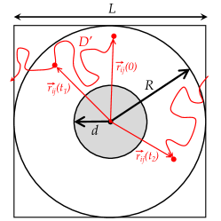
Figure 1: Schematic representation of a random walker $j$ travelling with a diffusion coefficient $D^{\prime}$ within the frame of reference of a particle $i$ (located at the origin) with and without periodic boundary conditions. The shaded volume with radius $d$ (distance of closest approach) marks the region avoided by random walker $j$. The sphere with radius $R$ indicates the volume, where starting positions $\vec{r}_{j}(0)$ with $r_{ij}(0)\!>\!d$ are sampled from if periodic boundary conditions are not applied. For random walker simulations with periodic boundary conditions, the starting positions are uniformly sampled from the entire box volume with box-size $L$ applying the condition $r_{ij}(0)\!>\!d$.

III Methods

III.1 Random Walker Monte Carlo Simulations

Here we outline our use of random walker Monte Carlo simulations exploring the diffusion-based contribution to the NMR dipolar relaxation with and without periodic boundary conditions (PBCs). The random walker simulations without PBCs are designed to match the conditions of the theory outlined by Hwang and Freed Hwang and Freed (1975). The simulations are carried out within the frame of reference of particle $i$, which hence stays fixed at the origin of the coordinate system. The diffusion coefficient $D^{\prime}$ therefore represents inter-diffusion coefficients of both particles $i$ and $j$ with $D^{\prime}=D_{i}+D_{j}$. As illustrated in Figure 1, if no PBCs are considered, the starting position of the random walker $\vec{r}_{j}(0)$ are sampled from the distance interval between $d\!<\!r_{ij}(0)\!<\!R$ along the $z$-axis using a $r^{-2}$ weighting. To represent a proper volume sampling, contributions from each individual trajectory are correspondingly weighted by a factor $r^{4}_{ij}(0)$. This realization of “importance sampling” strongly reduces the statistical noise compared to the unbiased volume sampling, in particular for large values of $R$. For simulations with PBCs, however, the starting positions are sampled uniformly from the volume of the cubic box with box-size $L$ while obeying the condition $r_{ij}(0)\!>\!d$. At $t\!=\!0$ each walker starts from its randomly selected starting position $\vec{r}_{j}(0)$. New coordinates are computed for discrete time intervals $\delta t\!=\!10^{-3}$ time units from $\vec{r}_{j}(t+\delta t)=\vec{r}_{j}(t)+\vec{o}$, where $\vec{o}$ is a vector with random orientation and $|\vec{o}|=(6D^{\prime}\delta t)^{1/2}$. Trial positions that would end up within the spherical volume with radius $r_{ij}<d$ are reflected from the sphere and corrected such that they are compatible with the reflective boundary conditions used in the theory of Hwang and Freed. If used, periodic boundary conditions are applied in the sense that the diffusing particle, when leaving the box on one side, will enter on the opposite side, as illustrated in Figure 1. Dipole-dipole correlation functions reported here are computed by sampling over $10^{8}$ individual trajectories.

III.2 MD Simulations

We have performed MD simulations of liquid water using the TIP4P/2005 model Abascal and Vega (2005), which has been demonstrated to rather accurately describe the properties of water compared to other simple rigid nonpolarizable water models.Vega and Abascal (2011) The simulations are carried out at $273\,\mbox{K}$ and $298\,\mbox{K}$ under $NVT$ conditions using system-sizes of 512, 1024, 2048, 4096, and 8192 molecules. The chosen densities correspond to a pressure of $1\,\mbox{bar}$ at the respective temperatures. MD simulations of 1 ns length each were performed using Gromacs 5.0.6.van der Spoel et al. (2005); Hess et al. (2008) The integration time step for all simulations was $2\,\mbox{fs}$. The temperature of the simulated systems was controlled employing the Nosé-Hoover thermostat S.Nosé (1984); Hoover (1985) with a coupling time $\tau_{T}\!=\!1.0\,\mbox{ps}$. Both, the Lennard-Jones and electrostatic interactions were treated by smooth particle mesh Ewald summation.Essmann et al. (1995); Wennberg et al. (2013, 2015) The Ewald convergence parameter was set to a relative accuracy of the Ewald sum of $10^{-5}$ for the Coulomb- and $10^{-3}$ for the LJ-interaction. All bond lengths were kept fixed during the simulation run and distance constraints were solved by means of the SETTLE procedure.Miyamoto and Kollman (1992)

To compute the intermolecular magnetic dipole-dipole correlation functions, many autocorrelation functions over relatively large time sets have to be computed with a high time resolution of $10\,\mbox{fs}$. To evaluate time correlation functions for large time sets with $10^{5}$ entries efficiently, we applied the convolution theorem using fast Fourier transformation (FFT).Grigera (2020); Press et al. (1992) The computations of the properties from MD simulations were done using our home-built software package MDorado based on the MDAnalysis Michaud-Agraval et al. (2011); Gowers et al. (2016), NumPy Oliphant (06), and SciPy Virtanen et al. (2020) frameworks. MDorado is available via Github.

IV Results and Discussion

IV.1 Intermolecular Dipole-Dipole Relaxation: Random Walker Monte Carlo Simulations and the Theory of Hwang and Freed

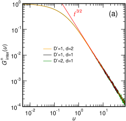
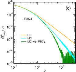
Figure 2: Normalized intermolecular dipole-dipole correlation functions $G^{\mathrm{n}}_{\mathrm{inter}}(u)$ computed from random walker models plotted on a reduced time-scale $u\!=\!D^{\prime}t/d^{2}$. a) $G^{\mathrm{n}}_{\mathrm{inter}}(u)$ computed with a sampling cutoff radius $R\!=\!100$ length units for different distances of closest approach $d$ and inter-diffusion coefficients $D^{\prime}$. Shown in red is also the long-time limiting $\lim_{u\rightarrow\infty}G^{\mathrm{n}}_{\mathrm{inter}}(u)\!\propto\!t^{-3/2}$ behavior following Equation 18. b) The orange line indicates $G^{\mathrm{n,HF}}_{\mathrm{inter}}(u)$ according to Equation 15. It is showing a $t^{-3/2}$-scaling behavior for long times according to Equation 18 indicated in red. Applying a cutoff for the starting positions of the random walkers affects the computed $G^{\mathrm{n,MC}}_{\mathrm{inter}}(u)$ shown in turquoise. These functions are depending on the chosen ratio of cutoff radius and distance of closest approach $R/d$. For long times the $G^{\mathrm{n,MC}}_{\mathrm{inter}}(u)$ exhibit a $t^{-5/2}$-scaling shown as green straight lines computed from Equation 25. c) The orange line indicates $G^{\mathrm{n,HF}}_{\mathrm{inter}}(u)$ according to Equation 15. Applying a cutoff for the starting positions of the random walkers affects the computed $G^{\mathrm{n,MC}}_{\mathrm{inter}}(u)$ shown in turquoise. The curves shown in green represent $G^{\mathrm{n,MC}}_{\mathrm{inter}}(u)$-functions that were computed applying periodic boundary conditions with starting positions sampled from a cubic box with box-length $L$ for comparable ratios $R/d=L/(2d)=4$.

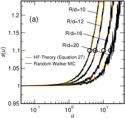
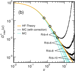
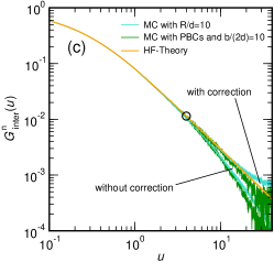
Figure 3: Corrections for $G^{\mathrm{n}}_{\mathrm{inter}}(u)$ obtained from simulations with a fixed sampling cutoff $R$ or periodic boundary conditions. Open symbols indicate $G^{\mathrm{n,HF}}_{\mathrm{inter}}(u_{\mathrm{tr}})$ with $u_{\mathrm{tr}}=R^{2}/(8\pi d^{2})$ or $u_{\mathrm{tr}}=L^{2}/(32\pi d^{2})$. a) Computed scaling functions $s(u)$ for various selected ratios $R/d$ employing a lower integration limit of the HF-function with $x_{\textrm{P}}\!=\!\theta\cdot d/R$ according to Equation 27 using $\theta\!=\!2.53$. b) Orange line: $G^{\mathrm{n,HF}}_{\mathrm{inter}}(u)$ representing the Hwang-Freed theory. Turquoise lines: $G^{\mathrm{n,MC}}_{\mathrm{inter}}(u)$ computed from random walker MC simulations for various ratios $R/d$. black lines: corrected $G^{\mathrm{n}}_{\mathrm{inter}}(u)=G^{\mathrm{n,MC}}_{\mathrm{inter}}(u)\cdot s(u,x_{P})$. c) Normalized intermolecular dipole-dipole correlation functions $G^{\mathrm{n}}_{\mathrm{inter}}(u)$. Orange line: Hwang-Freed theory $G^{\mathrm{n,HF}}_{\mathrm{inter}}(u)$. Turquoise lines: Data obtained from random walker MC simulations with $R/d=10$ with and without correction according to Equation 27. Green lines: Data obtained from random walker MC simulations with periodic boundary conditions with $L/(2d)=10$ with and without correction according to Equation 27.

Let us consider the normalized intermolecular dipole-dipole correlation function $G^{\mathrm{n}}_{\mathrm{inter}}(t)=G_{\mathrm{inter}}(t)/G_{\mathrm{inter}}(0)$ computed from the random walker Monte Carlo simulations shown in Figure  2a for varying inter-diffusion coefficients $D^{\prime}$ and distances of closest approach $d$. Here we introduce a reduced timescale $u$ based on $d$ and $D^{\prime}$ using

$$u\equiv\frac{D^{\prime}t}{d^{2}}\;.$$ (14)

Employing the timescale $u$, all $G^{\mathrm{n}}_{\mathrm{inter}}(u)$ computed from random walkers for varying parameters $D^{\prime}$ and $d$ collapse on the same curve as shown in Figure 2a. Following the approach of Hwang and Freed Hwang and Freed (1975), we can also give an analytical integral expression for the dipole-dipole correlation function of two diffusing particles with a distance of closest approach $d$, reflecting boundary conditions at $r=d$, and an inter-diffusion coefficient $D^{\prime}$. The corresponding normalized correlation function on the reduced timescale $u$ is given by

$$G^{\mathrm{n,HF}}_{\mathrm{inter}}(u)=\frac{1}{A}\;\int\limits_{0}^{\infty}\frac{x^{2}\cdot e^{-u\cdot x^{2}}\;dx}{81+9x^{2}-2x^{4}+x^{6}}\;,$$ (15)

where $x$ represents a reduced inverse distance scale $x\equiv d/r$. The constant $A$ follows from computing the integral for $u\!=\!0$ with

$$A=\int\limits_{0}^{\infty}\frac{x^{2}\;dx}{81+9x^{2}-2x^{4}+x^{6}}=\frac{\pi}{54}\;.$$ (16)

For other values of $u$ this integral needs to be evaluated either numerically or by using the analytically integrated form derived by Hwang and Freed via partial fractions.Hwang and Freed (1975) For the purpose of our paper, however, the integral form given in Equation 15 turns out to be particularly useful. Note also that for short times $u$ the function $G^{\mathrm{n}}_{\mathrm{inter}}(u)$ can be expressed via a first-order expansion of the exponential function and is hence showing a linear time dependence with

$$\lim_{u\rightarrow 0}G^{\mathrm{n,HF}}_{\mathrm{inter}}(u)\approx 1-9u\;.$$ (17)

However, this linear time dependence may not properly represent molecular processes in liquids, since the corresponding time regime will more likely be dominated by oscillatory and jump-like motions. This is in accordance with the observation of Sholl, who has pointed out that the exact functional form of the high frequency limit of the intermolecular spectral density is highly sensitive to the employed motional model.Sholl (1981) For long times, ultimately, $G^{\mathrm{n,HF}}_{\mathrm{inter}}(t)$ exhibits a $t^{-3/2}$ scaling behavior and can be expressed using the reduced time-scale $u$ as

$$\lim_{u\rightarrow\infty}G^{\mathrm{n,HF}}_{\mathrm{inter}}(u)\approx\frac{1}{6\sqrt{\pi}\cdot u^{3/2}}\;.$$ (18)

The accurate description of the $t^{-3/2}$ long-time limiting behavior of $G^{\mathrm{n}}_{\mathrm{inter}}(t)$ by means of MD simulations is particularly important for properly describing the low frequency limit of the corresponding spectral density function $\lim_{\omega\rightarrow 0}J^{\mathrm{HF}}_{\mathrm{inter}}(\omega)\propto\sqrt{\omega}$, which can be utilised to extract the inter-diffusion coefficient from the slope of frequency-dependent relaxation rate $\lim_{\omega\rightarrow 0}R_{1}(\omega)$ vs. $\sqrt{\omega}$ Hwang and Freed (1975). Using the normalized dipole-dipole correlation function of the Hwang and Freed theory according to Equation 15, the full intermolecular spectral density of a random walker is given by

$$J^{\mathrm{HF}}_{\mathrm{inter}}(\omega_{u}) = \frac{2}{5}\left<\sum_{j}r^{-6}_{ij}(0)\right>\cdot J^{\mathrm{n,HF}}_{\mathrm{inter}}(\omega_{u})\;.$$ (19)

Here $J^{\mathrm{n,HF}}_{\mathrm{inter}}(\omega_{u})$ denotes the “normalized” Hwang-Freed spectral density, obtained as a Fourier transformation of $G^{\mathrm{n}}_{\mathrm{inter}}(t)$ with

$$J^{\mathrm{n,HF}}_{\mathrm{inter}}(\omega_{u}) = \frac{54}{\pi}\cdot\frac{d^{2}}{D^{\prime}}\int\limits_{0}^{\infty}\mathrm{Re}\left\{\int\limits_{0}^{\infty}e^{-u\cdot x^{2}}\;e^{i\omega_{u}u}\;du\right\}$$

$$\times\,\frac{x^{2}\;dx}{81+9x^{2}-2x^{4}+x^{6}}$$

and

$$J^{\mathrm{n,HF}}_{\mathrm{inter}}(\omega_{u}) = \frac{54}{\pi}\cdot\frac{d^{2}}{D^{\prime}}$$

$$\times\int\limits_{0}^{\infty}\frac{dx}{(81+9x^{2}-2x^{4}+x^{6})(1+\omega_{u}^{2}/x^{4})}\;,$$

where $\omega_{u}\equiv\omega\cdot d^{2}/D^{\prime}$ denotes a reduced frequency scale, corresponding to the reduced time scale $u$. From Equation IV.1 follows directly the spectral density in the extreme narrowing limit as

$$J^{\mathrm{HF}}_{\mathrm{inter}}(0) = \frac{2}{5}\left<\sum_{j}r^{-6}_{ij}(0)\right>\cdot\frac{4}{9}\cdot\frac{d^{2}}{D^{\prime}}\;,$$ (22)

where

$$\tau_{\mathrm{G,HF}}\!=\!J^{\mathrm{n,HF}}_{\mathrm{inter}}(0)\!=\!\frac{4}{9}\cdot\frac{d^{2}}{D^{\prime}}$$ (23)

represents the intermolecular dipole-dipole “correlation-time” obtained as integral over the normalized dipole-dipole correlation function $G^{\mathrm{n,HF}}_{\mathrm{inter}}(t)$. The limiting behavior of the “normalized” spectral density given by Equation IV.1 for small frequencies is characterized by a $\omega^{1/2}$ dependence according to

$$\lim_{\omega_{u}\rightarrow 0}J^{\mathrm{n,HF}}_{\mathrm{inter}}(\omega_{u})\approx J^{\mathrm{n,HF}}_{\mathrm{inter}}(0)-\frac{\sqrt{2}}{6}\cdot\frac{d^{2}}{D^{\prime}}\cdot\sqrt{\omega_{u}}\;.$$ (24)

The Hwang and Freed theory outlined above describes the behavior of ideal random walkers characterized by infinitely long diffusion paths sampled from an infinitely large system. In computer simulations of condensed matter systems, however, we mostly deal with finite system sizes using periodic boundary conditions. These conditions impose the following two problems: 1) they limit the volume from which the starting positions are sampled from, and, 2) the trajectories are altered by box-shifting, if not unwrapped. Unwrapping the trajectories, however, has the unfortunate tradeoff of drastically reducing the accuracy of the computed short-time behavior Busch, Neumann, and Paschek (2021) by not allowing the particles to reconvene. Both problems can be countered by increasing the system size, but they still might persist to some level. To thoroughly study and quantify both phenomena, we show in Figure  2b the dipole-dipole correlation functions computed from Monte Carlo simulations with very short cutoff radii $R/d\leq 4$. Note that both depicted correlation functions show a strong deviation from the Hwang-Freed model for $t\rightarrow\infty$. This deviation is due a systematic depletion of particles at long times $t$, and is related to the lack of particles arriving from starting distances with $r_{ij}(0)>R$, leading to an entirely different scaling behavior at long times. The computed $G^{\mathrm{n}}_{\mathrm{inter}}(u)$ scales with the square of ratio $(R/d)^{2}$ and approaches a $t^{-5/2}$ long-time limiting behavior according to

$$\lim_{u\rightarrow\infty}G^{\mathrm{n}}_{\mathrm{inter}}(u,R/d)\approx\frac{1}{a\cdot u^{5/2}}\cdot\left(\frac{R}{d}\right)^{2}$$ (25)

with $a\approx 23.6$. When PBCs are introduced, another effect comes into play: if a particle is leaving the box and entering the box on the opposite side, it is basically changing its identity. If this identity change is ignored, the consequence is a change in the direction of the vector connecting these two particles due to the mechanisms of the “minimum image convention” Allen and Tildesley (1987), which has obviously ramifications for the computed dipole-dipole correlation function $G^{\mathrm{n}}_{\mathrm{inter}}(u)$. As can be seen in the green solid curve shown in Figure 2c, this mechanism even enhances the effect due to the restricted sampling volume and leads to an even stronger deviation of the computed $G^{\mathrm{n}}_{\mathrm{inter}}(u)$ from the $t^{-3/2}$-behavior. The example of $R/d\!=\!L/(2d)\!=\!4$ shown in Figure 2c roughly corresponds to a rather small but not unrealistic system size of about 128 water molecules, according to the parameters given in Table 1 for $273\,\mbox{K}$. From Figure 2c it is also evident, however, that for sufficiently small times (such as $u\approx 1$), the additional deviation according to the periodic boundary conditions is practically negligible compared to the effect due to the limited sampling volumes.

In the following, we would like to derive a procedure to determine up to which time interval we can actually trust the computed intermolecular dipolar correlation functions despite the presence of periodic boundary conditions and limited sampling volumes. To approximate the effect caused to the limited sampling volumes on the correlation function according to the Hwang and Freed model given in Equation 15, we use a nonzero lower boundary value $x_{\mathrm{P}}\!=\!\theta\cdot d/R$ with $\theta\!\approx\!2.53$ for the integral of Equation 15, leading to

$$G^{\mathrm{n,HF}}_{\mathrm{inter}}(u,x_{\mathrm{P}})=\frac{1}{A(x_{\mathrm{P}})}\;\int\limits_{x_{\mathrm{P}}}^{\infty}\frac{x^{2}\cdot e^{-u\cdot x^{2}}\;dx}{81+9x^{2}-2x^{4}+x^{6}}\;,$$ (26)

realising that the variable $x$ is essentially representing an inverse distance. Here the parameter $\theta$ has been determined empirically to provide the best agreement with our random walker simulations for various values of $R/d$. Note that the normalisation constant $A(x_{\mathrm{P}})$ needs to be computed by numerical integration, except for $A(x_{\mathrm{P}}\!=\!0)=\pi/54$. The deviation of the approximate expression given by Equation 26 from Equation 15 can then be quantified by

$$s(u,x_{\mathrm{P}})=\frac{G^{\mathrm{n,HF}}_{\mathrm{inter}}(u,x_{\mathrm{P}}\!=\!0)}{G^{\mathrm{n,HF}}_{\mathrm{inter}}(u,x_{\mathrm{P}})}\;,$$ (27)

where the denominator represents Equation 15. As shown in Figure 3a, Equation 27 very well captures the initial effect due to the limited sampling volumes over a broad range of $R/d$ values that would correspond to liquid water simulations ranging from 2000 to about 16000 water molecules in a cubic unit cell. However, as shown in Figure 3b, for longer times, correcting the Monte Carlo simulation data via $s(u,x_{\mathrm{P}})$ leads to an overcorrection, suggesting that the introduction of a certain time-limit $t_{\mathrm{tr}}$ is necessary, up to which the correction could be meaningfully applied. Realising that the corresponding timescale is governed by the ratio of the radius $R$ (or the half box size $L/2$) and the inter-diffusion coefficient $D^{\prime}$, we use here

$$t_{\mathrm{tr}}=\frac{R^{2}}{8\pi D^{\prime}}=\frac{L^{2}}{32\pi D^{\prime}}\,,$$ (28)

which will consistently result in a time range where the scaling function $s(u,x_{\mathrm{P}})\leq 1.1$, as shown in Figure 3a. Employing the definition of the reduced timescale, we get

$$u_{\mathrm{tr}}=\frac{1}{8\pi}\cdot\frac{R^{2}}{d^{2}}=\frac{1}{32\pi}\cdot\frac{L^{2}}{d^{2}}\,,$$ (29)

indicating that the trusted time interval is just defined by the ratio $R/d$ (or $L/(2d)$). As shown in Figure 3c, when considering times $t\leq t_{\mathrm{tr}}$ the deviation introduced additionally due to the effect of periodic boundary conditions can be practically neglected.

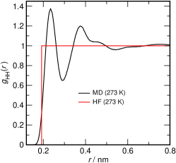
Figure 4: Intermolecular H-H radial distribution function $g_{\mathrm{HH}}(r)$ as a function of distance $r$ for $273\,\mbox{K}$ in addition to the corresponding step-like $g_{\mathrm{HH}}(r)$ according to the Hwang and Freed theory with a distance of closest approach of $d_{\mathrm{HH}}\!=\!0.192\,\mbox{nm}$.

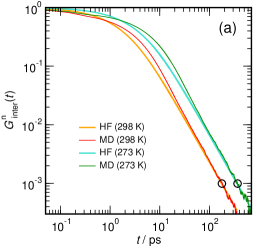
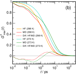
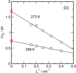
Figure 5: Normalized intermolecular dipole-dipole correlation functions $G^{\mathrm{n}}_{\mathrm{inter}}(t)$ computed for TIP4P/2005 water for $273\,\mbox{K}$ and $298\,\mbox{K}$. Red and green lines: $G^{\mathrm{n,MD}}_{\mathrm{inter}}(t)$ are obtained from MD simulations containing 8192 water molecules. Corrections according to Equation 27 are applied. Orange and turquoise lines $G^{\mathrm{n,HF}}_{\mathrm{inter}}(t)$ computed using data shown in Table 1. Open circles: $t_{\mathrm{tr}}\!=\!L^{2}/(32\pi D^{\prime})$ Dashed lines: difference functions $\Delta G^{\mathrm{n}}_{\mathrm{inter}}(t)=G^{\mathrm{n,MD}}_{\mathrm{inter}}(t)-G^{\mathrm{n,HF}}_{\mathrm{inter}}(t)$. a) Log-log plot. b) Linear-log plot c) Scaling of the computed intermolecular $\Delta\tau_{\mathrm{G}}$ given in Table 1 as a function of the inverse box length $L^{-1}$, analogous to the scaling of the translational diffusion coefficient suggested by Yeh and Hummer Yeh and Hummer (2004). Extrapolated values for $L\!\rightarrow\!\infty$ are indicated in red.

Table 1: Parameters describing the intermolecular dipolar NMR relaxation from MD simulations under $NVT$ conditions at the indicated densities $\rho$ and temperatures $T$. $L$: MD unit cell box-length. $d_{\mathrm{HH}}$: Distance of closest approach computed from H-H pair distribution functions including a long-range correction. $D_{\text{E}}$: “Einstein” water self-diffusion coefficient, determined from the slope of the center-of-mass mean square displacement of the water molecules (slope fitted to time interval between $15\,\mbox{ps}$ and $200\,\mbox{ps}$). $D_{0}$: water self-diffusion coefficient including the Yeh-Hummer finite-size correction Yeh and Hummer (2004) for systems with periodic boundary conditions $D_{0}\!=\!D_{\text{E}}+k_{\mathrm{B}}T\zeta/(6\pi\eta L)$ with $\zeta\approx 2.837297$ and $\eta$ the shear viscosity ($0.855\,\mbox{mPa\,s}$ at $298\,\mbox{K}$ and $1.76\,\mbox{mPa\,s}$ at $273\,\mbox{K}$ Gonzáles and Abascal (2010)). Inter-diffusion coefficient used for the correction: $D^{\prime}\!=\!2D_{\text{E}}$. Maximum time interval up to which the computed and corrected dipolar correlation function can be trusted: $t_{\mathrm{tr}}\!=\!L^{2}/(32\pi D^{\prime})$. Deviation of the total dipole-dipole correlation time from the Hwang-Freed model: $\Delta\tau_{\text{G}}$. It is obtained by numerically integrating the difference $\Delta G^{\mathrm{n}}_{\mathrm{inter}}(t)=G^{\mathrm{n,MD}}_{\mathrm{inter}}(t)-G^{\mathrm{n,HF}}_{\mathrm{inter}}(t)$ up to time $t_{\mathrm{tr}}$. Total intermolecular dipole-dipole correlation time: $\tau_{\text{G}}\!=\!(4/9)\,d_{\mathrm{HH}}^{2}/(2D_{0})+\Delta\tau_{\text{G}}$.

$N$	$T/\text{K}$	$\rho/\text{g}\,\text{cm}^{-3}$	$L/\text{nm}$	$d_{\mathrm{HH}}/\mathrm{\AA}$	$L/(2d)$	$D_{\text{E}}/10^{-9}\,\text{m}^{2}\text{s}^{-1}$	$D_{0}/10^{-9}\,\text{m}^{2}\text{s}^{-1}$	$t_{\mathrm{tr}}/\mbox{ps}$	$\Delta\tau_{\mathrm{G}}/\text{ps}$	$\tau_{\text{G}}/\text{ps}$
512	273	0.9997	2.48368	1.92	6.47	0.98	1.11	$62.6$	0.69	8.07
1024	273	0.9997	3.12924	1.92	8.15	1.01	1.11	$86.2$	0.89	8.27
2048	273	0.9997	3.94259	1.92	10.3	1.03	1.11	$150$	1.06	8.44
4096	273	0.9997	4.96735	1.92	12.9	1.05	1.11	$234$	1.23	8.61
8192	273	0.9997	6.25847	1.92	16.3	1.06	1.11	$368$	1.25	8.63
$\infty$	273	0.9997	$\infty$	1.92	$\infty$	1.11	1.11	$\infty$	1.68	9.06
512	298	0.9972	2.48582	1.93	6.44	2.01	2.30	$30.6$	0.41	4.01
1024	298	0.9972	3.13194	1.93	8.11	2.08	2.31	$46.9$	0.49	4.07
2048	298	0.9972	3.94600	1.93	10.2	2.12	2.31	$73.1$	0.52	4.10
4096	298	0.9972	4.97165	1.93	12.9	2.16	2.31	$114$	0.57	4.15
8192	298	0.9972	6.26388	1.93	16.2	2.19	2.31	$178$	0.61	4.19
$\infty$	298	0.9972	$\infty$	1.93	$\infty$	2.31	2.31	$\infty$	0.73	4.31

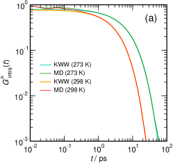
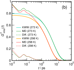
Figure 6: Normalized intramolecular dipole-dipole correlation functions $G^{\mathrm{n}}_{\mathrm{intra}}(t)$ computed for TIP4P/2005 water for $273\,\mbox{K}$ and $298\,\mbox{K}$. Red and green lines: $G^{\mathrm{n,MD}}_{\mathrm{intra}}(t)$ are obtained from MD simulations containing 8192 water molecules. Orange and turquoise lines: KWW functions $G^{\mathrm{n,K}}_{\mathrm{intra}}(t)$ according to Equation 35 computed using data shown in Table 2. a) Log-log plot. b) Linear-log plot including difference functions (dashed lines) $\Delta G^{\mathrm{n}}_{\mathrm{intra}}(t)=G^{\mathrm{n,MD}}_{\mathrm{intra}}(t)-G^{\mathrm{n,K}}_{\mathrm{intra}}(t)$.

Table 2: Parameters describing the intramolecular dipolar NMR relaxation from MD simulations. Due to the fixed intramolecular distance $r_{\mathrm{HH}}\!=\!1.514\,\mbox{\AA}$ in the TIP4P/2005 water model, the computed intramolecular dipole-dipole correlation functions are equivalent to the reorientational correlation functions of the intramolecular H–H vector. The computed $G^{\mathrm{n,MD}}_{\mathrm{intra}}(t)$ are fitted to a Kohlrausch-Williams-Watts (KWW) function with $G^{\mathrm{n,K}}_{\mathrm{intra}}(t)\!=\!A_{\mathrm{K}}\cdot\exp[-(t/\tau_{\mathrm{K}})^{\beta_{\mathrm{K}}}]$. The fit is performed for data within a time window between $1\,\mbox{ps}$ and $100\,\mbox{ps}$. The integrated correlation time of the KWW function is given as $\tau_{\mathrm{G,K}}\!=\!A_{\mathrm{K}}\tau_{\mathrm{K}}\beta^{-1}_{\mathrm{K}}\Gamma(\beta^{-1}_{\mathrm{K}})$, where $\Gamma(\ldots)$ represents the Gamma-function. Deviation of the total dipole-dipole correlation time from the KWW function: $\Delta\tau_{\text{G}}$. It is obtained by numerically integrating the difference $\Delta G^{\mathrm{n}}_{\mathrm{intra}}(t)=G^{\mathrm{n,MD}}_{\mathrm{intra}}(t)-G^{\mathrm{n,K}}_{\mathrm{intra}}(t)$ up to a time of $5\,\mbox{ps}$. Total intramolecular dipole-dipole correlation time: $\tau_{\text{G}}\!=\tau_{\mathrm{G,K}}+\Delta\tau_{\text{G}}$.

$N$	$T/\text{K}$	$A_{\mathrm{K}}$	$\tau_{\mathrm{K}}/\mathrm{ps}$	$\beta_{\mathrm{K}}$	$\tau_{\mathrm{G,K}}/\mathrm{ps}$	$\Delta\tau_{\mathrm{G}}/\mbox{ps}$	$\tau_{\text{G}}/\mbox{ps}$
512	273	0.800	6.12	0.886	5.20	0.024	5.22
1024	273	0.811	6.12	0.866	5.34	0.021	5.35
2048	273	0.795	6.32	0.892	5.31	0.028	5.34
4096	273	0.798	6.31	0.886	5.34	0.028	5.37
8192	273	0.799	6.30	0.884	5.35	0.028	5.38
512	298	0.779	3.06	0.908	2.50	0.006	2.51
1024	298	0.767	3.07	0.916	2.45	0.029	2.48
2048	298	0.771	3.02	0.908	2.44	0.031	2.47
4096	298	0.778	2.99	0.899	2.45	0.025	2.48
8192	298	0.772	3.03	0.907	2.45	0.028	2.48

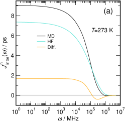
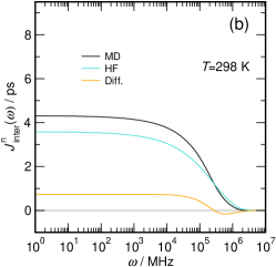
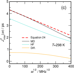
Figure 7: Intermolecular spectral density $J^{\mathrm{n}}_{\mathrm{inter}}(\omega)$ computed for TIP4P/2005 water for a) $273\,\mbox{K}$ and b) $298\,\mbox{K}$. Black lines: $J^{\mathrm{n,MD}}_{\mathrm{inter}}(\omega)$. Turquoise lines: $J^{\mathrm{n,HF}}_{\mathrm{inter}}(\omega)$, computed using data shown in Table 1 for $N\rightarrow\infty$. Orange lines: difference functions $\Delta J^{\mathrm{n}}_{\mathrm{inter}}(\omega)=J^{\mathrm{n,MD}}_{\mathrm{inter}}(\omega)-J^{\mathrm{n,HF}}_{\mathrm{inter}}(\omega)$, obtained by Fourier transformation of $\Delta G^{\mathrm{n}}_{\mathrm{inter}}(t)$ from MD simulations containing 8192 water molecules. c) Intermolecular spectral density obtained for $298\,\mbox{K}$ as a function of $\sqrt{\omega}$. Red dashed line: Low-frequency limiting behavior $\lim_{\omega\rightarrow 0}J^{\mathrm{n,HF}}_{\mathrm{inter}}(\omega)$ according to Equation 24.

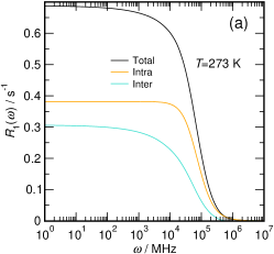
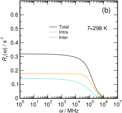
Figure 8: Frequency-dependent intermolecular, intramolecular, and total dipole-dipole ¹H NMR relaxation rates computed for TIP4P/2005 water according to Equations IV.2 and IV.2 for a) $273\,\mbox{K}$ and b) $298\,\mbox{K}$.

Table 3: Intermolecular, Intramolecular, and total dipolar ¹H NMR relaxation rates in the extreme narrowing limit computed for the TIP4P/2005 water model. Intramolecular H-H distance of the TIP4P/2005 model used for computing the intramolecular relaxation rate: $r_{\mathrm{HH}}\!=\!1.514\,\mbox{\AA}$. Experimental relaxation rates were obtained by Krynicki Krynicki (1966). Goldammer and Zeidler v. Goldammer and Zeidler (1969) studied mixtures of water with organic compounds to separate intra- from intermolecular contributions. Calero et al.Calero, Martí, and Guàrdia (2015) computed inter- and intramolecular relaxation rates from MD simulations of the TIP4P/2005 water model.

$N$	$T/\text{K}$	$R_{1,\mathrm{inter}}(0)/\mbox{s}^{-1}$	$R_{1,\mathrm{intra}}(0)/\mbox{s}^{-1}$	$R_{1}(0)/\mbox{s}^{-1}$
512	273	0.272	0.370	0.642
1024	273	0.279	0.380	0.659
2048	273	0.285	0.379	0.664
4096	273	0.291	0.381	0.672
8192	273	0.292	0.382	0.674
$\infty$	273	0.306	0.382	0.688
Expt.Krynicki (1966)	273	–	–	0.578
512	298	0.133	0.178	0.311
1024	298	0.135	0.176	0.311
2048	298	0.136	0.175	0.311
4096	298	0.138	0.176	0.314
8192	298	0.139	0.176	0.315
$\infty$	298	0.143	0.176	0.319
Expt.v. Goldammer and Zeidler (1969); Krynicki (1966)	298	0.110	0.170	0.280
MDCalero, Martí, and Guàrdia (2015)	298	0.087	0.176	0.263

Table 4: Intermolecular, Intramolecular, and total dipolar ¹H NMR relaxation rates as a function of the frequency $\omega$ computed for the TIP4P/2005 water model.

$\omega/\mbox{MHz}$	$T/\text{K}$	$R_{1,\mathrm{inter}}(\omega)/\mbox{s}^{-1}$	$R_{1,\mathrm{intra}}(\omega)/\mbox{s}^{-1}$	$R_{1}(\omega)/\mbox{s}^{-1}$
0	273	0.306	0.382	0.688
50	273	0.301	0.382	0.683
200	273	0.296	0.382	0.678
400	273	0.292	0.382	0.674
800	273	0.286	0.382	0.668
1200	273	0.281	0.382	0.663
0	298	0.143	0.176	0.319
50	298	0.141	0.176	0.317
200	298	0.140	0.176	0.316
400	298	0.138	0.176	0.314
800	298	0.136	0.176	0.312
1200	298	0.135	0.176	0.311

IV.2 Using a Mixed Theory/MD Approach to Compute the Frequency-Dependent NMR Relaxation of ¹H Nuclei in Liquid Water

We have performed $NVT$ MD simulations of TIP4P/2005 water at $273\,\mbox{K}$ and $298\,\mbox{K}$ at respective densities of $0.9997\,\text{g}\,\text{cm}^{-3}$ and $0.9972\,\text{g}\,\text{cm}^{-3}$, corresponding to an average pressure of about $1\,\mbox{bar}$ for system sizes between 512 and 8192 molecules. Data characterizing the simulations can be found in Table 1. We have computed the self-diffusion coefficients using the Einstein formula Allen and Tildesley (1987) according to

$$D_{\textrm{E}}=\frac{1}{6}\frac{\partial}{\partial t}\lim_{t\rightarrow\infty}\left<|\mathbf{r}(0)-\mathbf{r}(t)|^{2}\right>\;,$$ (30)

where $\mathbf{r}(t)=[r_{x}(t),r_{y}(t),r_{z}(t)]$ represents the position of the center of mass of a water molecule at time $t$. All computed self-diffusion coefficients shown Table 1 were determined from the slope of the mean square displacement of the water molecules fitted to time intervals between $15\,\mbox{ps}$ and $200\,\mbox{ps}$. Note that the $D_{\textrm{E}}$ is a system size dependent quantity, which can, however, be corrected via Dünweg and Kremer (1993); Yeh and Hummer (2004)

$$D_{0}=D_{\text{E}}+\frac{k_{\mathrm{B}}T\zeta}{6\pi\eta L}\;,$$ (31)

with the box size $L$, and the shear viscosity $\eta$. Here, $D_{0}$ is the system size independent true self-diffusion coefficient obtained for $L\rightarrow\infty$, $k_{\mathrm{B}}$ represents Boltzmann’s constant and $T$ is the temperature. The parameter $\zeta\!\approx\!2.837297$ is the analogue to a Madelung constant Beenakker (1986) of a cubic lattice, which can be computed via Ewald summation.Beenakker (1986); Hasimoto (1959) All computed values for $D_{0}$ are also given in Table 1. To perform the correction, we have employed the shear viscosity $\eta$ of $0.855\,\mbox{mPa\,s}$ at $298\,\mbox{K}$ and $1.76\,\mbox{mPa\,s}$ at $273\,\mbox{K}$ reported by Ref. Gonzáles and Abascal (2010). The distances of closest approach $d_{\mathrm{HH}}$ for the ¹H nuclei given in Table 1 for $273\,\mbox{K}$ and $289\,\mbox{K}$ are determined by integrating the $r^{-6}$ weighted H-H radial distribution functions according to Equations 11 and 13. The numerical integration of the pair correlation function was performed up to a distance of $L/2$ and was improved by adding a term for the long-range correction of $32\pi/(3L^{3})$. Note the slight temperature dependence of the computed $d_{\mathrm{HH}}$. Both the radial distribution function $g_{\mathrm{HH}}(r)$ obtained from MD and according to the Hwang Freed theory are shown in Figure 4 for $273\,\mbox{K}$.

To determine the intermolecular dipolar relaxation correlation functions $G^{\mathrm{n,MD}}_{\mathrm{inter}}(t)$, we have computed an average over $512\times(N-1)$ intermolecular correlation functions where $N$ is the number of molecules, leading to a total of 4193792 correlation functions for the 8192 molecule system. For the calculation, we have used one H-atom per water molecule. In Figure 5a we are comparing the time dependence of the normalized intermolecular dipole-dipole correlation functions $G^{\mathrm{n,MD}}_{\mathrm{inter}}(t)$ computed directly from molecular simulations including the correction according to Equation 27 with the prediction of the Hwang and Freed model $G^{\mathrm{n,HF}}_{\mathrm{inter}}(t)$ employing the distances of closest approach $d_{\mathrm{HH}}$ and the inter-diffusion coefficients $D^{\prime}=2D_{\mathrm{E}}$ obtained for a system size of 8192 water molecules. The values for the computed trusted time-intervals $t_{\mathrm{tr}}$ are indicated by open circles and are also given in Table 1 for all system sizes and temperatures. For times $t\approx t_{\mathrm{tr}}$ the function shows a $t^{-3/2}$ scaling behavior and the curve determined from MD simulation asymptotically approaches the Hwang and Freed model. For times $t\geq t_{\mathrm{tr}}$ both curves are practically indistinguishable. A log-linear representation of the data, including the difference function

$$\Delta G^{\mathrm{n}}_{\mathrm{inter}}(t)=G^{\mathrm{n,MD}}_{\mathrm{inter}}(t)-G^{\mathrm{n,HF}}_{\mathrm{inter}}(t)$$ (32)

is shown in Figure 5b. Note that the difference function is negative up to a time of about $1\,\mbox{ps}$, then turns positive until it asymptotically approaches zero. The negative region is due to fast librational motions of the water molecules, whereas the positive region is related due to a resting tendency of the protons after large angular jumps. In total, both the negative and positive deviation from an overall continuous diffusion of the ¹H nuclei, as described by the Hwang-Freed model, are reflecting the jump-like reorientational dynamics of water molecules discussed in detail by D. Laage and J.T. Hynes.Laage and Hynes (2006, 2008) The intermolecular correlation time $\tau_{\mathrm{G}}$ can be computed as an integral over $G^{\mathrm{n,MD}}_{\mathrm{inter}}(t)$, which can be splitted into two terms according to

$$\tau_{\mathrm{G}}=\tau_{\mathrm{G,HF}}+\Delta\tau_{\mathrm{G}}$$ (33)

with $\tau_{\mathrm{G,HF}}=9/4\cdot d_{\mathrm{HH}}/D^{\prime}$ following Equation 23. Here $\Delta\tau_{\mathrm{G}}$ can be computed comfortably via numerical integration of

$$\Delta\tau_{\mathrm{G}}\approx\int\limits_{0}^{t_{\mathrm{tr}}}\Delta G^{\mathrm{n}}_{\mathrm{inter}}(t)\;dt$$ (34)

due to the short-time nature of $\Delta G^{\mathrm{n}}_{\mathrm{inter}}(t)$. Computed values for $\Delta\tau_{\mathrm{G}}$ and $\tau_{\mathrm{G}}$ are listed in Table 1 for all temperatures and system sizes. Note that the inter-diffusion coefficients used for determining $\tau_{\mathrm{G,HF}}$ are based here on the system size dependent diffusion coefficients $D^{\prime}=2D_{\mathrm{E}}$ shown in Table 1. This is a necessary requirement, since otherwise $\Delta G^{\mathrm{n,MD}}_{\mathrm{inter}}(t)$ and $\Delta G^{\mathrm{n,HF}}_{\mathrm{inter}}(t)$ would not match at long times. As a consequence, $\Delta\tau_{\mathrm{G}}$ shows a system size dependence, as it is indicated in Figure 5c. Here, the apparent linear dependence from the inverse box length is purely based on empirical evidence. The rationale for an increase of $\Delta\tau_{\mathrm{G}}$ is based on the fact that the initial decay of $G^{\mathrm{n,MD}}_{\mathrm{inter}}(t)$ is largely due to the mutual reorientational motions of adjacent molecules and that that dynamics of these reorientational motions is nearly system size independent Celebi et al. (2021), thus increasing the net-positive difference between $G^{\mathrm{n,MD}}_{\mathrm{inter}}(t)$ and $G^{\mathrm{n,HF}}_{\mathrm{inter}}(t)$ with increasing system size. Based on the apparent linear $L^{-1}$-dependence, we can also give an estimate for $\Delta\tau_{\mathrm{G}}$ for $L\rightarrow\infty$. In combination with the true self-diffusion coefficient $D_{0}$, we can give an estimate for the true system size independent correlation time $\tau_{\mathrm{G}}$ shown in Table 1, and can thus also give an estimate for the true intermolecular relaxation rate $\lim_{L\rightarrow\infty}R_{\mathrm{inter}}(0)$.

To describe the intramolecular dipolar relaxation, we essentially compute the reorientational motion of the H-H vector, since the H-H distance of $r_{\mathrm{HH}}=0.1514\,\mbox{nm}$ is fixed within the TIP4P/2005 water model. Here the computed $G^{\mathrm{n,MD}}_{\mathrm{intra}}(t)$ represent averages over all $N$ intramolecular H-H vectors. In principle, we choose to follow the same strategy for the intramolecular dipolar correlation as we did for the intermolecular dynamics. The main difference, however, is that we do not employ a physics-based mechanistic model, but choose to apply the empricial Kohlrausch-Williams Watts (KWW) function for describing the long time behavior

$$G^{\mathrm{n,K}}_{\mathrm{intra}}(t)=A_{\mathrm{K}}\cdot\exp\left[-\left(\frac{t}{\tau_{\mathrm{K}}}\right)^{\beta_{\mathrm{K}}}\right]\;.$$ (35)

This empirical model is fitted to the computed $G^{\mathrm{n,MD}}_{\mathrm{intra}}(t)$ over a time interval between $1\,\mbox{ps}$ and $100\,\mbox{ps}$. In Figure 6a both functions are plotted and they become pretty much indistinguishable for times $t$ larger than about $2\,\mbox{ps}$. The fitted parameters are summarized in Table 2. A log-linear representation of the data, including the difference function

$$\Delta G^{\mathrm{n}}_{\mathrm{intra}}(t)=G^{\mathrm{n,MD}}_{\mathrm{intra}}(t)-G^{\mathrm{n,K}}_{\mathrm{intra}}(t)$$ (36)

is shown in Figure 6b. Significant differences between $G^{\mathrm{n,MD}}_{\mathrm{intra}}(t)$ and $G^{\mathrm{n,K}}_{\mathrm{intra}}(t)$ are restricted to a time-interval $t\leq 1\,\mbox{ps}$. Hence the intramolecular correlation time $\tau_{\mathrm{G}}$ was computed as an integral over $G^{\mathrm{n,MD}}_{\mathrm{intra}}(t)$, which can be splitted into two terms according to

$$\tau_{\mathrm{G}}=\tau_{\mathrm{G,K}}+\Delta\tau_{\mathrm{G}}$$ (37)

with

$$\tau_{\mathrm{G,K}}\!=\!A_{\mathrm{K}}\tau_{\mathrm{K}}\beta^{-1}_{\mathrm{K}}\Gamma(\beta^{-1}_{\mathrm{K}})\;,$$ (38)

where $\Gamma(\ldots)$ represents the Gamma-function. The deviation of the total dipole-dipole correlation time from the KWW function $\Delta\tau_{\text{G}}$ is obtained by numerically integrating the difference $\Delta G^{\mathrm{n}}_{\mathrm{intra}}(t)$ according to Equation 37 up to a time of $5\,\mbox{ps}$. Both the fitted parameters and the computed total correlation time $\tau_{\mathrm{G}}$ shown in Table 2 obtained for various system sizes do not indicate any system size dependence, which is in accordance with the finding of Celebi et al. Celebi et al. (2021) who noticed that the finite size correction for the rotational diffusion scales with the inverse box volume and is therefore much smaller than the one for translational diffusion.

Next, we want to compute the frequency-dependent spectral densities and thus the frequency-dependent relaxation rates. To compute the intermolecular spectral density from MD simulation, we use

$$J^{\mathrm{n,MD}}_{\mathrm{inter}}(\omega)=J^{\mathrm{n,HF}}_{\mathrm{inter}}(\omega)+\Delta J^{\mathrm{n}}_{\mathrm{inter}}(\omega)$$ (39)

with

$$\Delta J^{\mathrm{n}}_{\mathrm{inter}}(\omega)\approx\int\limits_{0}^{t_{\mathrm{tr}}}\Delta G^{\mathrm{n}}_{\mathrm{inter}}(\omega)\cos(\omega t)\;dt\;.$$ (40)

Here the integration in Equation 40 is performed numerically employing the trapezoidal rule up the time $t_{\mathrm{tr}}$, where both functions $G^{\mathrm{n,MD}}_{\mathrm{inter}}(\omega)$ and $G^{\mathrm{n,HF}}_{\mathrm{inter}}(\omega)$ are deemed indistinguishable. An important feature of this approach is that arbitrary frequencies $\omega$ can be used here, which is helpful in evaluating the relaxation rate, where both $J^{\mathrm{n,MD}}_{\mathrm{inter}}(\omega)$ and $J^{\mathrm{n,MD}}_{\mathrm{inter}}(2\omega)$ need to be computed. To properly predict $J^{\mathrm{n,MD}}_{\mathrm{inter}}(\omega)$ for systems with $L\rightarrow\infty$, we employ the system size independent self-diffusion coefficient $D_{0}$ for computing $J^{\mathrm{n,HF}}_{\mathrm{inter}}(\omega)$. In addition, we use

$$\Delta G^{\mathrm{n}}_{\mathrm{inter}}(\omega)\approx\frac{\tau_{\mathrm{G},N\rightarrow\infty}}{\tau_{\mathrm{G},N=8192}}\cdot\Delta G^{\mathrm{n}}_{\mathrm{inter},N=8192}(\omega)$$ (41)

to predict the behavior of $\Delta G^{\mathrm{n}}_{\mathrm{inter}}(\omega)$ for infinite system sizes. Here $\Delta G^{\mathrm{n}}_{\mathrm{inter},N=8192}(\omega)$ is the difference function computed for a system containing 8192 water molecules, and $\tau_{\mathrm{G},N=8192}=J^{\mathrm{n,MD}}_{\mathrm{inter},N=8192}(0)$ and $\tau_{\mathrm{G},N\rightarrow\infty}=J^{\mathrm{n,MD}}_{\mathrm{inter},N\rightarrow\infty}(0)$ are the corresponding correlation times predicted for an infinite system size via extrapolation shown in Table 1. The frequency depdendence of $J^{\mathrm{n,MD}}_{\mathrm{inter}}(\omega)$, $J^{\mathrm{n,HF}}_{\mathrm{inter}}(\omega)$, and $\Delta J^{\mathrm{n}}_{\mathrm{inter}}(\omega)$ are shown in Figure 7 for $273\,\mbox{K}$ and $298\,\mbox{K}$. Note that the low frequency-behavior of the intermolecular spectral density $\lim_{\omega\rightarrow 0}J^{\mathrm{n,HF}}_{\mathrm{inter}}(\omega)$ shown in Figure 7c follows a $\sqrt{\omega}$ dependence according to Equation 24 up to about $100\,\mbox{MHz}^{1/2}$, which corresponds to frequencies up to about $10\,\mbox{GHz}$, which is way beyond the frequency range accessible via currently available NMR technology. We can therefore conclude that frequency-dependent ¹H NMR relaxation observed experimentally for liquid water at $298\,\mbox{K}$ is largely dominated by translational diffusion. Note, however, that the dispersion of the computed $J^{\mathrm{n,MD}}_{\mathrm{inter}}(\omega)$ shown in Figure 7a and Figure 7b is markedly deviating from the behavior predicted by Hwang and Freed, showing a much sharper decay. This is the consequence of the negative part of the $\Delta J^{\mathrm{n}}_{\mathrm{inter}}(\omega)$-functions observed for frequencies $\omega\geq 1.5\times 10^{5}\,\mbox{MHz}$ and $\omega\geq 3\times 10^{5}\,\mbox{MHz}$ observed for $T\!=\!273\,\mbox{K}$ and $T\!=\!298\,\mbox{K}$, respectively. This spectral feature is obviously related to fast librational motions of the water molecules, in combination with large angular jumps, which are characterizing their reorientational motions.

Next, we would apply the same strategy outlined in the previous paragraph also to the intramolecular relaxation rate, and then combine both intra- and intermolecular contributions to describe the total ¹H relaxation. To compute the intramolecular spectral density from MD simulation, we use

$$J^{\mathrm{n,MD}}_{\mathrm{intra}}(\omega)=J^{\mathrm{n,K}}_{\mathrm{intra}}(\omega)+\Delta J^{\mathrm{n}}_{\mathrm{intra}}(\omega)$$ (42)

with

$$\Delta J^{\mathrm{n}}_{\mathrm{intra}}(\omega)\approx\int\limits_{0}^{t^{*}}\Delta G^{\mathrm{n}}_{\mathrm{intra}}(\omega)\cos(\omega t)\;dt\;.$$ (43)

Here the computation of the integral in Equation 43 is as well performed numerically, employing the trapezoidal rule up a time $t^{*}=5\mbox{ps}$, where both functions $G^{\mathrm{n,MD}}_{\mathrm{intra}}(\omega)$ and $G^{\mathrm{n,K}}_{\mathrm{intra}}(\omega)$ become effectively indistinguishable. The Fourier-transform of $G^{\mathrm{n,K}}_{\mathrm{intra}}(t)$, defined in Equation 35, $J^{\mathrm{n,K}}_{\mathrm{intra}}(\omega)$, needs, however, to be computed numerically, due to the lack of an analytical Fourier-transform equivalent of the KWW-function. To compute $J^{\mathrm{n,K}}_{\mathrm{intra}}(\omega)$ properly, we have tested the convergence of the numerical cosine-transform evaluation by comparing it to the limiting value for $\omega\rightarrow 0$ provided by the analytically obtained data given in Table 2. In Figure 8 we have plotted the inter- and intramolecular contribution to the ¹H NMR relaxation rate following Equation II computed via

$$R_{1,\mathrm{inter}}(\omega) = \gamma_{\mathrm{H}}^{4}\hbar^{2}\cdot\frac{3}{4}\cdot\left(\frac{\mu_{0}}{4\pi}\right)^{2}\cdot\frac{8\pi}{15}\cdot\frac{\rho_{\mathrm{H}}}{d_{\mathrm{HH}}^{3}}\times$$

$$\left\{J^{\mathrm{n,MD}}_{\mathrm{inter}}(\omega)+4\,J^{\mathrm{n,MD}}_{\mathrm{inter}}(2\omega)\right\}$$

and

$$R_{1,\mathrm{intra}}(\omega) = \gamma_{\mathrm{H}}^{4}\hbar^{2}\cdot\frac{3}{4}\cdot\left(\frac{\mu_{0}}{4\pi}\right)^{2}\cdot\frac{2}{5}\cdot\frac{1}{r_{\mathrm{HH}}^{6}}\times$$

$$\left\{J^{\mathrm{n,MD}}_{\mathrm{intra}}(\omega)+4\,J^{\mathrm{n,MD}}_{\mathrm{intra}}(2\omega)\right\}$$

as a function of the frequency $\omega$ over many orders of magnitude. Here $\rho_{\mathrm{H}}$ is representing the number density of the ¹H nuclei in liquid water. Note that for frequencies $\omega\leq 10^{3}\,\mbox{MHz}$ $R_{1,\mathrm{intra}}(\omega)$ is basically frequency independent, confirming that the dispersion that can be experimentally obtained is solely caused by the intermolecular contributions. In Table 3 we have listed the data for the inter-, intramolecular, and total dipolar ¹H NMR relaxation rates in the extreme narrowing limit $\omega\rightarrow 0$ computed for the TIP4P/2005 water model. Note that the computed relaxation rates are significantly larger than the experimental data. This might seem odd since the diffusion coefficient of the TIP4P/2005 model at $298\,\mbox{K}$ of $D_{0}=2.31\times 10^{-9}\,\mbox{m}^{2}\,\mbox{s}^{-1}$ matches almost perfectly the experimental value of $D_{0}=2.3\times 10^{-9}\,\mbox{m}^{2}\,\mbox{s}^{-1}$.Krynicki, Green, and Sawyer (1978) However, one has to keep in mind that the TIP4P/2005 model is a rigid model, and that additional high frequency bond-length and bond-bending motions, which the TIP4P/2005 model is lacking, will lead to a further quenching of both $G^{\mathrm{n,MD}}_{\mathrm{inter}}(t)$ and $G^{\mathrm{n,MD}}_{\mathrm{intra}}(t)$, leading to smaller inter- and intramolecular relaxation rates. Therefore it should not come as a surprise that the computed ¹H relaxation rates are larger than the experimental ones. It is, however, surprising that the ¹H relaxation rate computed by Calero et al. Calero, Martí, and Guàrdia (2015) for the TIP4P/2005 model is actually smaller than the experimental data of Krynicky Krynicki (1966). By using the data given in their paper, we have computed their intramolecular relaxation rate and found it to be in perfect agreement with our data (see Table 3). Their intermolecular relaxation rate of $0.087\,\mbox{s}^{-1}$, however, is even smaller than the value according to Hwang-Freed theory purely based on intermolecular diffusion of $0.119\;\mbox{s}^{-1}$ when using $D_{0}=2.31\times 10^{-9}\,\mbox{m}^{2}\,\mbox{s}^{-1}$ and $d_{\mathrm{HH}}=0.193\,\mbox{nm}$. This, however, seems rather unlikely and emphasizes the importance to properly consider the long-time nature of the $G^{\mathrm{n,MD}}_{\mathrm{inter}}(t)$ with its slowly decaying $t^{-3/2}$ time dependence.

Finally, in Table 4 we report data for the computed relaxation rates for TIP4P/2005 water for frequencies accessible via modern NMR hardware. The reduction of the total relaxation rate of $3.6\%$ at $273\,\mbox{K}$ and $2.5\%$ at $298\,\mbox{K}$ is purely due to changes in intermolecular relaxation rate. Of course, for supercooled liquid water, the effect of dispersion will increase substantially. Note that Krynicky determined the ¹H NMR relaxation rate of water at a frequency of $50\,\mbox{MHz}$.Krynicki (1966) The expected reduction of the relaxation rate due to intermolecular contributions of $0.7\%$ compared to the true extreme narrowing limit is, however, smaller than their reported experimental error of about $1\%$.

V Conclusion

We have introduced a computational framework aimed at accurately determining the frequency-dependent intermolecular NMR dipole-dipole relaxation rate of spin $1/2$ nuclei through MD simulations. This framework circumvents the influence of well-known finite-size effects on translational diffusion. Moreover, we have developed a method to manage and rectify the impacts stemming from fixed distance-sampling cutoffs and periodic boundary conditions.

Our approach is capable of accurately forecasting the proper low-frequency $\sqrt{\omega}$-scaling behavior of the intermolecular NMR dipole-dipole relaxation rate observed experimentally. It is based on the theory of Hwang and Freed Hwang and Freed (1975) for the intermolecular dipole-dipole relaxation and is utilizing their analytical expressions for both the dipole-dipole correlation function and its corresponding spectral density. Deviations from the Hwang and Freed theory caused by periodic boundary conditions and restrictions due to sampling distance cutoffs were studied and quantified by means of random walker Monte Carlo simulations. These simulation were designed to perfectly replicate the force free hard sphere model underlying the Hwang and Freed theory. Based on both the Hwang and Freed theory and the Monte Carlo simulations, an expression has been derived for correcting for those effects and to determine the time interval up to which the corrected correlation functions faithfully follow the true behavior observed, when restrictions due to sampling distance cutoffs and periodic boundary effects are absent.

As a proof of principle, our approach is demonstrated by computing the frequency-dependent inter- and intramolecular dipolar NMR relaxation rate of the ¹H nuclei in liquid water at $273\,\mbox{K}$ and $298\,\mbox{K}$ based on simulations of the TIP4P/2005 model. In particular, our calculations suggest that the intermolecular contribution to the ¹H relaxation rate of the TIP4P/2005 model in the extreme narrowing limit has been previously significantly underestimated.

Author Declarations

Conflict of Interest

The authors have no conflicts to disclose.

Author Contributions

Dietmar Paschek: Conceptualization (lead); Methodology (lead); Formal analysis (lead); Investigation (lead); Software (lead); Data curation (lead); Visualization (lead); Supervision (equal); Project administration (supporting); Writing – original draft (lead); Writing – review & editing (lead). Johanna Busch: Investigation (supporting); Software (supporting); Writing – review & editing (supporting). Eduard Mock: Software (supporting). Ralf Ludwig: Conceptualization (supporting); Resources (lead); Writing – review & editing (supporting). Anne Strate: Conceptualization (supporting); Funding acquisition (lead); Project administration (lead); Supervision (equal); Writing – review & editing (supporting).

Data Availability

The codes of GROMACS and MDorado are freely available. Input parameter and topology files for the MD simulations, the code for performing random walker Monte Carlo Simulations, and the code for computing intermolecular and intramolecular relaxation rates can be downloaded from GitHub via github.com/Paschek-Lab/DrelaxD.

References

- Abragam (1961) A. Abragam, The Principles of Nuclear Magnetism (Oxford University Press, 1961).
- Kowalewski (2013) J. Kowalewski, “Nuclear magnetic resonance,” (Royal Society of Chemistry, 2013) Chap. Nuclear spin relaxation in liquids and gases, pp. 230–275.
- Kruk, Meier, and Rössler (2011) D. Kruk, R. Meier, and A. Rössler, “Translational and rotational diffusion of glycerol by means of field cycling 1H NMR relaxometry,” J. Phys. Chem. B 115, 951–957 (2011).
- Kruk, Hermann, and Rössler (2012) D. Kruk, A. Hermann, and E. A. Rössler, “Field-cycling NMR relaxometry of viscous liquids and polymers,” Prog. Nucl. Magn. Reson. Spectrosc. 63, 33–64 (2012).
- Sholl (1981) C. A. Sholl, “Nuclear-spin relaxation by translational diffusion in liquids and solids - high-frequency and low-frequency limits,” J. Phys. C: Solid State Phys. 14, 447–464 (1981).
- Hwang and Freed (1975) L.-P. Hwang and J. H. Freed, “Dynamic effects of pair correlation functions on spin relaxation by translational diffusion in liquids,” J. Chem. Phys. 63, 4017–4025 (1975).
- Overbeck et al. (2020) V. Overbeck, B. Golub, H. Schröder, A. Appelhagen, D. Paschek, K. Neymeyr, and R. Ludwig, “Probing relaxation models by means of fast field-cycling relaxometry, NMR spectroscopy and molecular dynamics simulations: Detailed insight into the translational and rotational dynamics of a protic ionic liquid,” J. Mol. Liq. 319, 114207 (2020).
- Overbeck et al. (2021) V. Overbeck, A. Appelhagen, R. Rößler, T. Niemann, and R. Ludwig, “Rotational correlation times, diffusion coefficients and quadrupolar peaks of the protic ionic liquid ethylammonium nitrate by means of 1H fast field cycling NMR relaxometry,” J. Mol. Liq. 322, 114983 (2021).
- Westlund and Lynden-Bell (1987) P. Westlund and R. Lynden-Bell, “A molecular dynamics study of the intermolecular spin-spin dipole-dipole correlation function of liquid acetonitrile,” J. Magn. Reson. 72, 522–531 (1987).
- Schnitker and Geiger (1987) J. Schnitker and A. Geiger, “NMR-quadrupole relaxation of Xenon-131 in water. a molecular dynamics simulation study,” Z. Phys. Chem. 155, 29–54 (1987).
- Yeh and Hummer (2004) I.-C. Yeh and G. Hummer, “System-size dependence of diffusion coefficients and viscosities from molecular dynamics simulations with periodic boundary conditions,” J. Phys. Chem. B 108, 15873–15879 (2004).
- Moultos et al. (2016) O. A. Moultos, Y. Zhang, I. O. Tsimpanogiannis, I. G. Economou, and E. J. Maginn, “System-size corrections for self-diffusion coefficients calculated from molecular dynamics simulations: The case of CO2, n-alkanes, and poly(ethylene glycol) dimethyl ethers,” J. Chem. Phys. 145, 074109 (2016).
- Busch and Paschek (2023) J. Busch and D. Paschek, “OrthoBoXY: A simple way to compute true self-diffusion coefficients from MD simulations with periodic boundary conditions without prior knowledge of the viscosity,” J. Phys. Chem. B 127, 7983–7987 (2023).
- Honegger et al. (2021) P. Honegger, M. E. Di Pietro, F. Castiglione, C. Vaccarini, A. Quant, O. Steinhauser, C. Schröder, and A. Mele, “The intermolecular NOE depends on isotope selection: Short range vs. long range behavior,” J. Phys. Chem. Lett. 12, 8658–8663 (2021).
- Abascal and Vega (2005) J. L. F. Abascal and C. Vega, “A general purpose model for the condensed phases of water: TIP4P/2005,” J. Chem. Phys. 123, 234505 (2005).
- Calero, Martí, and Guàrdia (2015) C. Calero, J. Martí, and E. Guàrdia, “1H nuclear spin relaxation of liquid water from molecular dynamics simulations,” J. Phys. Chem. B 119, 1966–1973 (2015).
- Odelius et al. (1993) M. Odelius, A. Laaksonen, M. H. Levitt, and J. Kowalewski, “Intermolecular dipole-dipole relaxation. a molecular dynamics simulation,” J. Magn. Reson. Ser. A 105, 289–294 (1993).
- Hertz (1967) H. G. Hertz, “Microdynamic Behaviour of Liquids as studied by NMR Relaxation Times,” Prog. NMR Spec. 3, 159–230 (1967).
- Hertz and Tutsch (1976) H. G. Hertz and R. Tutsch, “Model Orientation Dependent Pair Distribution Functions Describing the Association of Simple Caboxyle Acids and of Ethanol in Aqueous Solution,” Ber. Bunsenges. Phys. Chem. 80, 1268–1278 (1976).
- Stejksal et al. (1959) E. O. Stejksal, D. E. Woessner, T. C. Farrar, and H. S. Gutowsky, “Proton magnetic resonance of the group. V. temperature dependence of in several molecular crystals,” J. Chem. Phys. 31, 55–65 (1959).
- Egelstaff (1992) P. A. Egelstaff, An Introduction to the Liquid State, 2nd ed. (Oxford University Press, Oxford, 1992).
- Vega and Abascal (2011) C. Vega and J. L. F. Abascal, “Simulating water with rigid non-polarizable models: a general perspective,” Phys. Chem. Chem. Phys. 13, 19633–19688 (2011).
- van der Spoel et al. (2005) D. van der Spoel, E. Lindahl, B. Hess, G. Groenhof, A. E. Mark, and H. J. C. Berendsen, “GROMACS: fast, flexible, and free,” J. Comput. Chem. 26, 1701–1718 (2005).
- Hess et al. (2008) B. Hess, C. Kutzner, D. van der Spoel, and E. Lindahl, “Gromacs 4: algorithms for highly efficient, load-balanced, and scalable molecular simulation,” J. Chem. Theory Comput. 4, 435–447 (2008).
- S.Nosé (1984) S.Nosé, “A molecular dynamics method for simulations in the canonical ensemble,” Mol. Phys. 52, 255–268 (1984).
- Hoover (1985) W. G. Hoover, “Canonical dynamics: Equilibrium phase-space distributions,” Phys. Rev. A 31, 1695–1697 (1985).
- Essmann et al. (1995) U. Essmann, L. Petera, M. Berkowitz, T. Darden, H. Lee, and L. Pedersen, “A smooth particle mesh ewald method,” J. Chem. Phys. 103, 8577–8593 (1995).
- Wennberg et al. (2013) C. L. Wennberg, T. Murtola, B. Hess, and E. Lindahl, “Lennard-jones lattice summation in bilayer simulations has critical effects on surface tension and lipid properties,” J. Chem. Theory Comput. 9, 3527–3537 (2013).
- Wennberg et al. (2015) C. L. Wennberg, T. Murtola, S. Páll, M. J. Abraham, B. Hess, and E. Lindahl, “Direct-space corrections enable fast and accurate lorentz-berthelot combination rule lennard-jones lattice summation,” J. Chem. Theory Comput. 11, 5737–5746 (2015).
- Miyamoto and Kollman (1992) S. Miyamoto and P. A. Kollman, “Settle: An analytical version of the shake and rattle algorithm for rigid water models,” J. Comput. Chem. 13, 952–962 (1992).
- Grigera (2020) T. S. Grigera, “Everything you wish to know about correlations but are afraid to ask,” arXiv:2002.01750v1 [cond-mat.stat-mech] (2020).
- Press et al. (1992) W. H. Press, S. A. Teukolsky, W. T. Vetterling, and P. Flannery, Numerical Recipes in C: The Art of Scientific Computing, 2nd ed. (Cambridge University Press, Cambridge, USA, 1992).
- Michaud-Agraval et al. (2011) N. Michaud-Agraval, E. J. Denning, T. B. Woolf, and O. Beckstein, “MDAnalysis: A toolkit for the analysis of molecular dynamics simulations,” J. Comput. Chem. 32, 2319–2327 (2011).
- Gowers et al. (2016) R. J. Gowers, M. Linke, J. Barnoud, T. J. E. Reddy, M. N. Melo, S. L. Seyler, J. Domański, D. L. Dotson, S. Buchoux, I. M. Kenney, and O. Beckstein, “MDAnalysis: A python package for the rapid analysis of molecular dynamics simulations,” in Proceedings of the 15th Python in Science Conference, edited by S. Benthall and S. Rostrup (Austin, TX, 2016) pp. 98–105.
- Oliphant (06 ) T. Oliphant, “NumPy: A guide to NumPy,” USA: Trelgol Publishing (2006–).
- Virtanen et al. (2020) P. Virtanen, R. Gommers, T. E. Oliphant, M. Haberland, T. Reddy, D. Cournapeau, E. Burovski, P. Peterson, W. Weckesser, J. Bright, S. J. van der Walt, M. Brett, J. Wilson, K. J. Millman, N. Mayorov, A. R. J. Nelson, E. Jones, R. Kern, E. Larson, C. J. Carey, İ. Polat, Y. Feng, E. W. Moore, J. VanderPlas, D. Laxalde, J. Perktold, R. Cimrman, I. Henriksen, E. A. Quintero, C. R. Harris, A. M. Archibald, A. H. Ribeiro, F. Pedregosa, P. van Mulbregt, and SciPy 1.0 Contributors, “SciPy 1.0: Fundamental Algorithms for Scientific Computing in Python,” Nature Methods 17, 261–272 (2020).
- Busch, Neumann, and Paschek (2021) J. Busch, J. Neumann, and D. Paschek, “An exact a posteriori correction for hydrogen bond population correlation functions and other reversible geminate recombinations obtained from simulations with periodic boundary conditions. liquid water as a test case,” J. Chem. Phys. 154, 214501 (2021).
- Allen and Tildesley (1987) M. P. Allen and D. J. Tildesley, Computer Simulation of Liquids (Oxford University Press, Clarendon, Oxford, 1987).
- Gonzáles and Abascal (2010) M. Gonzáles and J. Abascal, “The shear viscosity of rigid water models,” J. Chem. Phys. 132, 096101 (2010).
- Krynicki (1966) K. Krynicki, “Proton spin-lattice relaxation in pure water between 0∘C and 110∘C,” Physica 32, 167–178 (1966).
- v. Goldammer and Zeidler (1969) E. v. Goldammer and M. D. Zeidler, “Molecular motion in aqueous mixtures with organic liquids by nmr relaxation measurements,” Ber. Bunsenges. Phys. Chem. 73, 4–15 (1969).
- Dünweg and Kremer (1993) B. Dünweg and K. Kremer, “Molecular dynamics simulation of a polymer chain in solution,” J. Chem. Phys. 99, 6983–6997 (1993).
- Beenakker (1986) C. W. J. Beenakker, “Ewald sum of the Rotne-Prager tensor,” J. Chem. Phys. 85, 1581–1582 (1986).
- Hasimoto (1959) H. Hasimoto, “On the periodic fundamental solutions of the stokes equations and their application to viscous flow past a cubic array of spheres,” J. Fluid Mech. 5, 317–328 (1959).
- Laage and Hynes (2006) D. Laage and J. T. Hynes, “A molecular jump mechanism of water reorientation,” Science 311, 832–835 (2006).
- Laage and Hynes (2008) D. Laage and J. T. Hynes, “On the molecular mechanism of water reorientation,” J. Phys. Chem. B 112, 14230–14242 (2008).
- Celebi et al. (2021) A. T. Celebi, S. H. Jamali, A. Bardow, T. J. H. Vlugt, and O. A. Moultos, “Finite-size effects of diffusion coefficients computed from molecular dynamics: a review of what we have learned so far,” Mol. Simul. 47, 831–845 (2021).
- Krynicki, Green, and Sawyer (1978) K. Krynicki, C. D. Green, and D. W. Sawyer, “Pressure and temperature dependence of self-diffusion in water,” Faraday Discuss. Chem. Soc. 66, 199–208 (1978).