HARMONIOUS – Human-like reactive motion control and multimodal perception for humanoid robots

Abstract

For safe and effective operation of humanoid robots in human-populated environments, the problem of commanding a large number of Degrees of Freedom (DoF) while simultaneously considering dynamic obstacles and human proximity has still not been solved. We present a new reactive motion controller that commands two arms of a humanoid robot and three torso joints (17 DoF in total). We formulate a quadratic program that seeks joint velocity commands respecting multiple constraints while minimizing the magnitude of the velocities. We introduce a new unified treatment of obstacles that dynamically maps visual and proximity (pre-collision) and tactile (post-collision) obstacles as additional constraints to the motion controller, in a distributed fashion over surface of the upper-body of the iCub robot (with 2000 pressure-sensitive receptors). The bio-inspired controller: (i) produces human-like minimum jerk movement profiles; (ii) gives rise to a robot with whole-body visuo-tactile awareness, resembling peripersonal space representations. The controller was extensively experimentally validated, including a physical human-robot interaction scenario.

I Introduction

As robots are leaving safety fences and starting to share workspaces and even living spaces with humans, they need to function in dynamic and unpredictable environments. Highly redundant platforms like humanoid robots have the possibility of performing tasks even in the presence of many constraints and obstacles. Given the dynamic nature of obstacles and real-time constraints, reactive motion control rather than planning is the solution. The key to success is whole-body awareness drawing on dynamic fusion of multimodal sensory information, inspired by peripersonal space representations in humans.

We present a reactive motion controller that commands the upper body of the iCub humanoid robot (2x 7 Degrees of Freedom (DoF) in every arm; 3 torso DoF), whereby the two hands can have separate tasks in Cartesian space or a common task (see Fig.1). Unique to our approach, obstacles perceived in three different modalities—visual and proximity (pre-collision) and tactile (post-collision)—are dynamically aggregated and projected first onto locations on individual body parts and then remapped as constraints into the joint velocity space.

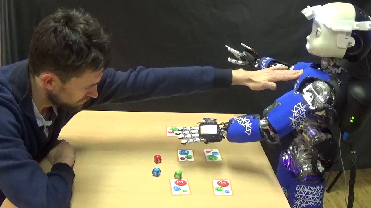
(a) The robot is approaching the correct card while back bending to dodge the collision.

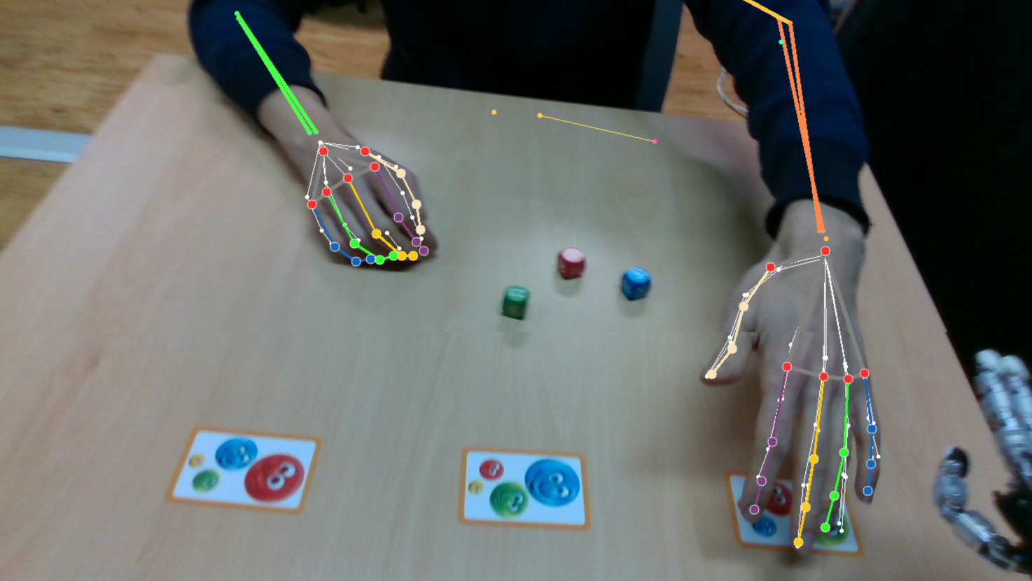
(b) The robot is keeping a safe distance from the opponent’s detected hand.

Figure 1: iCub robot in action during an interactive game demonstration.

I-A Inverse kinematics

With robot tasks are defined in Cartesian (also called operational or task) space while they are commanded in joint space, some form of inverse kinematics (IK) mapping ($\mathbf{q}=f(\mathbf{x})$) is indispensable. For industrial manipulators, a closed-form analytical solution is often available, especially for 6 DoF arms with a so-called spherical wrist. Closed-form solutions are global and fast to compute. However, such analytical solutions exploit specific geometric relationships and are in general not available for redundant robots with an arbitrary kinematic structure (but cf. [1]). Numerical approaches to IK come with a higher computational load, but are more general—applicable to any kinematic chain. TRAC-IK [2] is a state-of-the-art IK solver that solves IK as a sequential quadratic programming problem. Lloyd et al. [3] presented an IK algorithm that uses the third-order root finding method to increase the speed and robustness of finding IK solutions. The solution consists of a set of target joint angles only—smooth trajectory generation and execution has to be taken care of separately. Pattacini et al. [4] combined a trajectory generator, a non-linear IK solver, and a Cartesian controller to ensure human-like minimum jerk movements in both Cartesian and joint space. None of the above methods can handle dynamic obstacles in the workspace. An overview of the related work from this and the following sections is in Tab. I.

Work	Control problem	ROA	Sensory modalities to perceive obstacles	DoF shown	Singularities handling	NPR	OEM	ETS
Ours	DiffK - QP problem	LIC	3 - vision, proximity, touch	17	Velocity damping	Yes	Yes	Yes
[2]	IK - Sequential QP	-	-	15	No	No	Yes	No
[3]	IK - Jacobian based	-	-	16	Damped variant	No	Yes	No
[4]	IK - Nonlinear opt.	-	-	7	No	Yes	Yes	Yes
[5]	DiffK - Damped LS	LIC	0 - known obstacles	8	Damped LS	No	Yes	No
[6]	DiffK - Pseudoinverse	PF	0 - known obstacles	7	No	No	Yes	Yes
[7]	DiffK - Pseudoinverse	RV	1 - vision	7	No	No	No	No
[8]	DiffK - QP problem	LIC	0 - known obstacles	7	Maximize manipulability	No	Yes	No
[9]	DiffK - QP problem	LIC	2 - proximity, touch	7	Velocity damping	Yes	No	No
[10]	DiffK - QP problem	LIC	1 - proximity	7	Velocity damping	No	No	No
[11]	DiffK - QP problem	LIC	0 - known obstacles	7	No	No	Yes	No
[12]	DiffK - QP problem	-	-	12	Maximize manipulability	No	Yes	No
[13]	DiffK - QP problem	LIC	0 - known obstacles	6	No	No	Yes	No
[14]	IK - Nonlinear opt.	CF	0 - known obstacles	8	Maximize condition number	No	Yes	No
[15]	Operational space control	PF	0 - known obstacles	6	No	No	Yes	No
[16]	ERG + PD control	PF	1 - vision	7	No	No	Yes	No
[17]	IK - Nonlinear opt.	RV	2 - vision, touch	10	No	No	Yes	Yes

TABLE I: Comparison of different approaches to solving the IK problem. Control problem acronyms are: differential kinematics (DiffK), inverse kinematics (IK), quadratic programming (QP), least squares (LS), and explicit reference governor (ERG). Reactive obstacle avoidance (ROA) types are linear inequality constraint (LIC), self-motion (SM), potential field (PF), danger index (DI), repulsive vector (RV), and part of the cost function (CF). The last columns are natural position reward (NPR), orientation error minimization (OEM), and explicit trajectory sampling (ETS).

I-B Obstacle avoidance and differential kinematics

Collision avoidance in static environments can be resolved at a higher level by using trajectory optimization for robot motion planning [18, 19, 20]. However, currently, these methods cannot provide solutions for scenarios like humanoid robots interacting with dynamic human-populated environments in real time. The family of methods that alleviate the above-mentioned problems and that are gaining popularity recently rely on differential kinematics, i.e. the formulation of the operational space task in velocity space and a mapping between desired Cartesian velocity and joint velocity through the robot Jacobian. Differential kinematics, also referred to as Resolved-rate motion control (RRMC), dates back to Whitney [21]. This method is inherently local—depends on the current robot configuration and the corresponding Jacobian—and as it provides joint velocities, it can be directly employed for motion control (without separate trajectory generation).

Inverse differential kinematics methods rely on some form of Jacobian inverse ($\mathbf{\dot{q}}=\mathbf{J}^{-1}(\mathbf{q})\mathbf{\dot{x}}$), more often pseudo-inverse when $J$ is not square, like for redundant robots. The damped least squares (DLS) method [5, 6, 7] is preferred over Jacobian pseudo-inverse or transpose as it “dampens” the motions in the vicinity of kinematic singularities. To dodge obstacles in redundant robots, self-motion, i.e. the possibility to use the null space of the solution for additional tasks, is exploited [22, 23, 24, 25]. The advantage of these approaches is that the problem has a clear hierarchical structure that allows to set priorities. For example, Albini et al. [22] define obstacle avoidance as the primary task and the reaching target uses the null space. The disadvantage is the limited flexibility of the problem formulation in face of many (some dynamically appearing) constraints or their changing priorities.

Alternatively, the motion control task can be defined using the forward differential formulation, searching for joint velocities $\mathbf{\dot{q}}$ that best match desired Cartesian velocity of the end effector $\mathbf{\dot{x}}$, thus minimizing $||\mathbf{\dot{x}}-\mathbf{J}(\mathbf{q})\mathbf{\dot{q}}||$. To this end, it is possible to use quadratic programming (QP) optimization with a quadratic cost function and linear constraints [8, 9, 10, 11, 12, 13, 26]. To avoid singular configurations, two options are usually given: add manipulability maximization to the cost function [8, 12] or dampen joint velocities when close to singularities [9, 10, 27]. In addition, undesirable configurations can be avoided by extending the optimization cost function to motivate the robot to be close to the middle of the joint limits [9] or close to the robot resting position [4]. In the case of the QP problem, obstacles are represented as linear inequality constraints allowing motions in tangential directions improving target reachability [8, 9, 10].

Most of the mentioned works do not solve self-collisions explicitly. The exceptions are [10], where self-collisions are solved by adding additional obstacle points for robot links and the end effector, and [14], where a neural network is trained to favor configurations far from self-collision states. Unlike most of the mentioned controllers that presented solutions of the IK problem for a single-arm robot, Tong et al. [12] proposed a four-criterion-optimization coordination motion scheme for a dual-arm robot that deals with coordination constraints and physical constraints. However, their approach does not consider obstacle avoidance and the torso joints of the dual-arm robot.

To represent obstacles, artificial potential fields [15], where obstacles are repulsive surfaces that repel the robot from the obstacle, can be used [16, 28, 29]. Park et al. [6] presented a dynamic potential field for smoother avoidance movements. Repulsive vectors in Cartesian space are shown in [7] and later used in [17, 30].

I-C Human-like motion generation

Several controllers can work as explicit local trajectory generators for sampling the trajectory between the start and target pose. The algorithm in [29] combines control with path planning and can handle arbitrary desired velocity profiles for the robot. The Cartesian controller [4] produces human-like quasi-straight trajectories whose typical characteristic is to rely on minimum-jerk profiles. A reactive controller in [17, 30] uses the minimum-jerk trajectory sampling as in [4]. Suleiman [13] proposed an algorithm for implicit minimum jerk trajectories by replacing joint velocities by joint jerk as control parameters in the optimization problem.

I-D Sensing of obstacles and contacts

To make safe movement of a robot in a cluttered or human-populated environment possible, obstacles need to be perceived in real time and processed either before a collision happens or immediately after contact with the robot. We will focus on perception in the context of HRI.

To sense at a distance, RGB-D cameras are frequently adopted [7, 31, 32, 33, 34]. Depth information can be used to compute a set of spheres that represent obstacles [33] or to create a depth space representation that is used to generate repulsive vectors for the robot [7]. Magrini and De Luca [24] estimated the contact force based on the contact point detected by a Kinect sensor. Alternative visual sensing for obstacle detection are tracking systems that follow markers attached to specific body parts, e.g., a wrist [29] or arm joints and a head [16]. Aljalbout et al. [35] used a static RGB camera in simulation and trained a convolutional neural network for obstacle avoidance.

Collisions with a moving robot may be acceptable provided that the contact forces are within limits. Collisions need to be detected, located, identified (e.g., determining the forces), and, possibly following classification of the collision, reacted upon (e.g., stop, slow down, retract, etc.) [36]. Force/torque sensors within the robot structure, together with models of its dynamics, can be employed. Alternatively, contacts can be perceived through tactile sensors. We will focus on large area sensitive skins. Differently than when force/torque sensors are employed, collision localization/isolation is easier, even for multi-contacts. Cirillo et al. [23] developed a flexible skin, allowing measurement of contact position and three components of contact force. Calandra et al. [37] presented a data-driven method for fast and accurate prediction of joint torques from contacts detected by tactile skin. Albini et al. used robot skin feedback HRI [38] and robot control in a cluttered environment [22]. Kuehn and Haddadin [39] introduced an artificial Robot Nervous System, which integrates tactile sensation and reflex reactions into robot control through the concept of robot pain sensation. The pain-reflex movements, in combination with the new skins, can improve the human feeling of robots and their safety. Some large area sensitive skins have been safety-rated and are deployed in collaborative robot applications (see Airskin and the analysis of its effects in [40]).

Individual visual sensors—on the robot itself or in other locations in the workspace—are prone to occlusions (which can be mitigated by employing multiple sensors [41]). Large area tactile arrays are distributed over the whole robot body, but only respond after physical contact. Distributed proximity sensors provide an alternative—sensing at a small distance over the whole robot body. Proximity [9, 10] or tomographic [42] sensors can be used for collision anticipation and contactless motion guidance.

Typically, only one sensor type is used and the corresponding robot control is more or less dependent on the nature of the sensory information. Works combining distal and contact sensing, like vision and touch [31, 43] or proximity and touch [9] are scarce. Humans posses a dynamically established protective safety margin around the whole body, drawing on visuo-tactile interactions: Peripersonal space (PPS), e.g., [44]. Roncone et al. [43, 45] took inspiration in the PPS and implemented visuo-tactile receptive fields on a humanoid robot. Nguyen et al. [17, 30] deployed this in HRI to feed a reactive motion controller. As affordable and increasingly accurate sensors of different types are becoming ubiquitous, it is important and timely to develop a unified treatment of their signals such that they can be processed by a single motion controller. In this work we—to our knowledge for the first time—present a framework in which RGB-D, proximity, and tactile sensors are simultaneously processed, related to the complete robot body, and used to generate real-time constraints for a whole-body reactive motion controller.

I-E Proposed solution (HARMONIOUS) and contribution over state of the art

Here we present HARMONIOUS – Human-like reactive motion control and multimodal perception for humanoid robots. An overview is provided in Fig. 2. The core of the solution is the motion controller (red box) and the actual QP formulation (magenta) which is online fed by the target trajectory generator (blue box) and the constraints projected from obstacles (green box). A detailed description is provided in the Materials and Methods section. To the extent that this is possible, the main components of our solution are categorized and contrasted with representative works from the literature in Tab. I.

We formulate the control problem (second column in Tab. I) as a quadratic program in velocity space— employing differential kinematics, similarly to many recent works in this area [8, 9, 10, 11, 12, 13]. Reactive obstacle avoidance (ROA, second column) is implemented using linear inequality constraint (LIC). Importantly, this work is to our knowledge the first to employ three different sensory modalities (vision, proximity, touch), in a unified manner, to perceive and avoid obstacles (fourth column). The fifth column (DoF shown) lists the number of DoF employed in our approach and in the literature. HARMONIOUS handles kinematic singularities through velocity damping. The robot is rewarded for assuming a natural posture (NPR), unlike most of the works in the literature. HARMONIOUS can handle position and orientation targets (OEM) and samples the trajectory of end-effector positions (ETS), inspired by human reaching movements—quasi-straight trajectories with bell-shaped velocity profiles. On the other hand, the end-effector orientation sampling is calculated using a computer graphics method slerp for constant angular velocities, ensuring smooth rotations and the shortest path between initial and final orientations. In summary, HARMONIOUS employs state-of-the-art control problem and reactive obstacle avoidance formulation, but moves beyond the state of the art in providing a unified treatment of three different sensory modalities, the number of DoF controlled, and incorporation of natural position reward and orientation error minimization. Beyond what could fit in Tab. I, HARMONIOUS also features self-collision avoidance and the possibility of setting targets (tasks) for the two robot arms independently or jointly (bimanual task). To our knowledge, HARMONIOUS is unparalleled in the scale of the problem and the number of features it can tackle.

HARMONIOUS was tested against the most relevant solutions from related works [4, 8, 17] in simulation experiments without and with obstacles and achieved the best results. Then, it was verified with a real robot in several collision avoidance scenarios. Another experiment showed the successful cooperation of both arms in a safe bimanual task. Moreover, it was shown that the problem formulation can be easily extended with other task constraints. As the final evaluation, we tested HARMONIOUS in an interactive board game scenario with the human player dynamically perceived, simultaneously processing keypoints on its body, proximity signals, and physical contacts on the whole robot body.

II Materials and Methods

II-A Experimental setup

The experiments were conducted with the humanoid robot iCub ([46], see Fig. 1), specifically on its upper body with 17 degrees of freedom (DoF) consisting of two 7-DoF arms and a common 3-DoF torso. The robot was equipped with an RGB-D camera Intel RealSense D435 placed above his eyes to track obstacles in 3D, an artificial electronic skin [47] to detect contacts and their intensity, and two proximity sensor units [48] with time-of-flight sensors that improve perception in “blind spots” (back of hands).

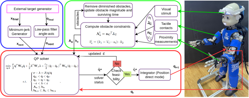
Figure 2: HARMONIOUS – overview. The blue box represents the local trajectory sampling. The trajectory towards the target pose is sampled using a minimum-jerk generator (position) and a low-pass filter (orientation). The target pose is received from an external target generator. The green box represents the obstacle processing. It takes inputs from proximity sensors, skin parts (tactile stimuli), and RGB-D camera (visual stimuli) and computes linear inequality constraints to dodge obstacles or react to the collision that occurred. The obstacle exists virtually for a specific survival time with decreasing threat level, giving humans time to react. The red box represents the controller with a QP solver that solves the differential kinematics problem. It takes the next desired pose and current joint positions as input. If the problem is feasible, the computed joint velocities are integrated into new joint positions and sent to the robot. Otherwise, the position constraint is relaxed, and the QP problem is solved again.

II-B Motion controller

The main component of our approach is a motion controller (see the red box in Fig. 2). Our motion controller is based on a reactive kinematic control, in particular the approach called differential kinematics which is defined as

$$\boldsymbol{\nu}=\mathbf{J}(\mathbf{q})\dot{\mathbf{q}}$$ (1)

where $\boldsymbol{\nu}$ is the spatial velocity of the end effector, $\dot{\mathbf{q}}$ are the joint velocities of the robot and $\mathbf{J}(\mathbf{q})$ is the Jacobian of the robot for the joint positions $\mathbf{q}$. This relation represents a trajectory constraint between robot configuration and Cartesian space.

The spatial velocity of the end effector is computed from the current end-effector pose and the desired end-effector pose in the next time period as

$$\boldsymbol{\nu^{pos}}=\frac{\mathbf{x_{t}}-\mathbf{x_{c}}}{t_{s}},\qquad\boldsymbol{\nu^{ori}}=\frac{\mathbf{R_{t}}\mathbf{R_{c}}^{T}}{t_{s}}$$ (2)

where $\boldsymbol{\nu^{pos}}$ is the translational velocity of the end effector, $\mathbf{x_{c}}$ and $\mathbf{x_{t}}$ are the current and desired next end effector position, $\boldsymbol{\nu^{ori}}$ is the rotational velocity of the end effector, $\mathbf{R_{c}}$ and $\mathbf{R_{t}}$ are the current and desired next end effector orientation, and $t_{s}$ is the period time.

For our purpose, we can relax the trajectory constraint by adding a slack variable $\boldsymbol{\lambda}$ to help the controller with finding a solution when other (e.g., safety) constraints appear:

$$\boldsymbol{\nu}-\boldsymbol{\lambda}=\mathbf{J}(\mathbf{q})\dot{\mathbf{q}}$$ (3)

Then, we formulate the problem as a strictly convex QP problem with joint velocities $\dot{\mathbf{q}}$ and slack variables $\boldsymbol{\lambda}$ as optimization variables. In our cost function, we minimize the sum of the squared Euclidean norm of the joint velocities, the distance from the natural joint positions, and the squared Euclidean norm of the vector of slack variables. It is formulated as:

$$\min_{\dot{\mathbf{q}},\boldsymbol{\lambda}}\ \frac{\mu}{2}\dot{\mathbf{q}}^{T}\mathbf{W_{q}}\dot{\mathbf{q}}+\frac{1}{2}\boldsymbol{\lambda}^{T}\mathbf{W_{\lambda}}\boldsymbol{\lambda}+\frac{c_{h}}{2}\left(\dot{\mathbf{q}}-\dot{\mathbf{q}}_{n}\right)^{T}\mathbf{W_{q}}\left(\dot{\mathbf{q}}-\dot{\mathbf{q}}_{h}\right)$$ (4)

where diagonal matrices $\mathbf{W_{q}}$ and $\mathbf{W_{\lambda}}$ contain the weights of the individual joints and the relaxations for the trajectory constrain, $\mathbf{\dot{q}}_{h}$ are the velocities needed to reach natural (home) robot configuration, $c_{h}$ is a weight of the motivation to keep robot close to his natural configuration, and $\mu$ is a damping factor calculated from the manipulability index $\omega=\sqrt{\mathbf{JJ}^{T}}$ [49] as:

$$\mu=\begin{cases}(1-\frac{\omega}{\omega_{0}})^{2}+0.01&\omega<\omega_{0},\quad\omega_{0}\text{ is a threshold,}\\ 0.01&\text{otherwise.}\end{cases}$$ (5)

This damping factor increases when the manipulability index decreases to zero, implying that the robot is close to a singularity position (the manipulability index is zero in that position). The higher damping factor makes the minimization of joint velocities more important, leading to lower joint velocities and singularity avoidance [27].

Apart from the mentioned relaxed trajectory constrained, the minimization is done with respect to several other constraints, such as joint velocity and position bounds (see Sec. II-K), slack variable bounds, collision avoidance (see Sec. II-F), and other task or kinematic constraints (see Sec. II-J). The constraints can be written as follows:

$$\mathrm{s.t.}\quad\begin{cases}\boldsymbol{\nu}-\boldsymbol{\lambda}=\mathbf{J}(\mathbf{q})\dot{\mathbf{q}}\\ \dot{\mathbf{q}}_{L}<\dot{\mathbf{q}}<\dot{\mathbf{q}}_{U}\\ \mathbf{q}_{L}<\mathbf{q}<\mathbf{q}_{U}\\ -\boldsymbol{\varepsilon}<\boldsymbol{\lambda}<\boldsymbol{\varepsilon}\\ \mathbf{A_{o}}\leq\mathbf{b_{o}}\\ \mathbf{b_{L,t}}\leq\mathbf{A_{t}}\leq\mathbf{b_{U,t}}\end{cases}$$ (6)

where $\mathbf{\dot{q}}_{L,U},\mathbf{q}_{L,U},\boldsymbol{\varepsilon}$ are the lower and upper bounds for the joint velocities, the joint positions, and the slack variables, respectively. $\mathbf{A_{o}}$ and $\mathbf{b_{o}}$ define obstacles avoidance constraints; $\mathbf{A_{t}}$, $\mathbf{b}_{L,t}$, and $\mathbf{b}_{U,t}$ define other task constraints.

II-C Dual-arm trajectory constraint

Here, we formulate the problem for two arms with a common torso. Since we have a common torso of the robot, we cannot calculate the trajectory constraints for the arms independently of each other. Moreover, it is not always possible to reach targets with both arms simultaneously, conflict situations are managed by prioritizing one of the arms and calling it the “primary arm”, and the other is then the “secondary arm”. Therefore, the trajectory constraint (Eq. 3) for a robot with a common torso is expanded as:

$$\begin{split}\boldsymbol{\nu_{p}^{pos}}-\boldsymbol{\lambda^{pos}_{p}}&=\mathbf{J_{t,pos}^{p}}(\mathbf{q^{t}})\mathbf{\dot{q}^{t}}+\mathbf{J_{a,pos}^{p}}(\mathbf{q^{p}})\mathbf{\dot{q}^{p}}\\ \boldsymbol{\nu_{p}^{ori}}-\boldsymbol{\lambda^{ori}_{p}}&=\mathbf{J_{t,ori}^{p}}(\mathbf{q^{t}})\mathbf{\dot{q}^{t}}+\mathbf{J_{a,ori}^{p}}(\mathbf{q^{p}})\mathbf{\dot{q}^{p}}\\ \boldsymbol{\nu_{s}^{pos}}-\boldsymbol{\lambda^{pos}_{s}}&=\mathbf{J_{t,pos}^{s}}(\mathbf{q^{t}})\mathbf{\dot{q}^{t}}+\mathbf{J_{a,pos}^{s}}(\mathbf{q^{s}})\mathbf{\dot{q}^{s}}\\ \boldsymbol{\nu_{s}^{ori}}-\boldsymbol{\lambda^{ori}_{s}}&=\mathbf{J_{t,ori}^{s}}(\mathbf{q^{t}})\mathbf{\dot{q}^{t}}+\mathbf{J_{a,ori}^{s}}(\mathbf{q^{s}})\mathbf{\dot{q}^{s}}\end{split}$$ (7)

where the subscripts $t,p,s$ represent torso, “primary arm”, and “secondary arm” respectively. The superscripts $pos,ori$ represent the relaxation of the constraint of the position and orientation trajectory, respectively. The single-arm formulation contains only the torso and the “primary arm” part. $\mathbf{J^{p/s}_{a,pos}}(\mathbf{q^{p/s}}),\mathbf{J^{p/s}_{t,pos}}(\mathbf{q^{t}})$ are the translational velocity components of the Jacobian matrices for arm and torso, respectively, $\mathbf{J^{p/s}_{a,ori}}(\mathbf{q^{p/s}}),\mathbf{J^{p/s}_{t,ori}}(\mathbf{q^{t}})$ are the rotational velocity components of the Jacobian matrices for arm and torso, respectively.

Consistent with the arm prioritization, we distinguish two cases for the limits of the slack variable $\boldsymbol{\varepsilon}$. They are set to $\infty$ (the deviation is minimized only) or to zero (the equality constraint without relaxation). In our solution, $\boldsymbol{\varepsilon}$ is set to $\infty$ for all $\boldsymbol{\lambda}$ except $\boldsymbol{\lambda_{p}^{pos}}=[0,0,0]^{T}$. If the equality constraint on the desired translation velocity of the “primary arm” makes the problem infeasible, we solve the problem again with the constraint relaxed to the minimization of the deviation. This strategy allows the robot to reach a target position with higher precision if the original problem is feasible and to make it feasible if the equality constraint is too strict.

II-D Local trajectory sampling

The first input to the reactive controller is the trajectory waypoint for the next time step (see the blue box in Fig. 2). Given the desired final target pose from an external source (e.g., a high-level target generator), we compute the desired next-time pose separately in position and orientation. We use a low-pass filter in the axis-angle representation for orientation sampling, which ensures a constant-speed transition between two orientations. For position sampling, a generator of approximately minimum-jerk trajectories is employed. Position samples are generated using a third-order linear time-invariant dynamical system [4].

We distinguish between streamed targets (e.g., reference tracking) and individual (reaching) targets. In the first case, the targets can be skipped (e.g., during collision avoidance), and only the newest one is important, and the local trajectory sampling is not applied as it is assumed that the movement smoothness is handled in the external target generator.

II-D1 Position sampling

The sampling of a time-varying input $\mathbf{x}_{d}\in\mathbb{R}^{3}$ expressing the desired positions for the end effector in Cartesian space is performed by means of a third-order filter, which is capable of generating output trajectories that exhibit the property of being quasi minimum-jerk, thus resembling the human-like movements as described in [50].

We tightly follow the implementation presented in [4], where the idea is to start from the feedback formulation of the minimum-jerk trajectory as the solution of the optimal problem proposed in [51]. The exact solution resorts to a third-order linear time-variant (LTV) dynamical filter applied to each coordinate $x_{d}\left(*\right)$ of the vector $\mathbf{x}_{d}$:

$$\begin{bmatrix}\dot{x}\cr\ddot{x}\cr\dddot{x}\end{bmatrix}=\begin{bmatrix}0&1&0\\ 0&0&1\\ \frac{-60}{\left(T-t\right)^{3}}&\frac{-36}{\left(T-t\right)^{2}}&\frac{-9}{T-t}\end{bmatrix}\begin{bmatrix}x\cr\dot{x}\cr\ddot{x}\end{bmatrix}+\begin{bmatrix}0\cr 0\cr\frac{60}{\left(T-t\right)^{3}}\end{bmatrix}x_{d}\left(*\right)$$ (8)

where $T$ represents the execution time.

To circumvent the difficulty posed by coefficients becoming unbounded for $t\rightarrow T$, the authors ran in [4] a second optimization to find out the third-order linear time-invariant (LTI) system that can deliver the best approximation of the output of Eq. 8, minimizing the jerk measure over the same temporal interval $\left[0,T\right]$.

The resulting LTI system is:

$$\begin{bmatrix}\dot{x}\cr\ddot{x}\cr\dddot{x}\end{bmatrix}=\begin{bmatrix}0&1&0\cr 0&0&1\cr\frac{a}{T^{3}}&\frac{b}{T^{2}}&\frac{c}{T}\end{bmatrix}\begin{bmatrix}x\\ \dot{x}\\ \ddot{x}\end{bmatrix}+\begin{bmatrix}0\\ 0\\ -\frac{a}{T^{3}}\end{bmatrix}x_{d}\left(*\right)$$ (9)

where $a\approx-150.766$, $b\approx-84.981$, and $c\approx-15.967$ are the constant coefficients found by the optimization, and $T$ is a parameter (related to the execution time) that regulates the reactivity of the filter. Throughout our experiments, we set $T=\left(||\mathbf{x_{d}}-\mathbf{x_{0}}||/v_{t}\right)$ s, where $\mathbf{x_{d}}$ is the desired target position, $\mathbf{x_{0}}$ is the starting position, and $v_{t}$ is the desired Cartesian speed of movement.

The output $\mathbf{x}\left(t\right)$ of the filter in Eq. 9 provides a sampling of the input $\mathbf{x}_{d}\left(t\right)$ that is “quasi” minimum-jerk, being the filter only an approximation of the system (Eq. 8), although we proved that it is reliable and effective in smoothing out sharp transitions while guaranteeing bell-shaped velocity profiles.

II-D2 Orientation sampling

We use the axis-angle representation for the orientations of the end effector. The orientation is described by a rotation vector $\mathbf{r}=\left[r_{1},r_{2},r_{3}\right]^{T},$ that encodes the axis of rotation $u=\mathbf{r}/||\mathbf{r}||$ and a rotation angle $\Theta=||\mathbf{r}||$. Orientation sampling is carried out by interpolation between two orientations $\mathbf{r_{1}},\mathbf{r_{2}}$ using a spherical linear interpolation, i.e., Slerp [52], which takes advantage of the fact that the spherical metric of $S^{3}$ is the same as the angular metric of $SO(3)$ for a constant angular speed of movement [52]. Moreover, it creates a torque-minimal path for the rotation as it travels along the straightest path the rounded surface of a sphere and it.

We first start by creating skew matrices $\mathbf{r_{+,1}},\mathbf{r_{+,2}}$ from rotation vectors $\mathbf{r_{1}},\mathbf{r_{2}}$ as

$$\mathbf{r_{+}}=\begin{bmatrix}0&-r_{3}&r_{2}\cr r_{3}&0&-r_{1}\cr-r_{2}&r_{1}&0\end{bmatrix}.$$

These matrices can be easily converted to rotation matrices $\mathbf{R_{1}},\mathbf{R_{2}}$ by computing their matrix exponentials (expm function):

$$\mathbf{R_{1}}=\mathrm{expm}(\mathbf{r_{+,1}}),\qquad\mathbf{R_{2}}=\mathrm{expm}(\mathbf{r_{+,2}})$$

We compute the interpolation between rotations $\mathbf{R_{1}},\mathbf{R_{2}}$ as

$$\mathrm{slerp}(\mathbf{R_{1}},\mathbf{R_{2}},\alpha)=\mathrm{expm}\left(\alpha\,\mathrm{logm}\left(\mathbf{R_{2}R_{1}^{T}}\right)\right)\mathbf{R_{1}},$$ (10)

where the function logm converts the rotation matrices to the skew matrices of the rotation vectors and $\alpha$ is an interpolation coefficient given as a period time $t_{s}$ divided by the trajectory time $T=\left(||\mathbf{x_{d}}-\mathbf{x_{0}}||/v_{t}\right)$ s. Finally, the computed rotations are converted back to the axis-angle representation.

II-E Peripersonal space projection

Roncone et al. [43, 45] proposed a distributed representation of the protective safety zone for humanoid robots, called Peripersonal space (PPS). The safety zone is represented by a collection of probabilities that an object from the environment eventually comes into contact with that particular skin taxel. For each taxel, they combined visual information of objects approaching the body and tactile information of eventual physical collision. A visual receptive field around the taxel is represented by a cone that rises from the surface along the normal.

Nguyen et al. [17, 30] made small modifications to PPS and used it to ensure safe interaction between humans and robots. Instead of training the visual receptive fields, they defined them uniformly for all taxels. In addition, they extended the reach of the receptive field to a maximum of 45 cm. Due to compatibility with the original implementation, the taxel receptive field has a discrete representation with 20 bins representing the distance from the obstacle with values of collision probabilities. The Parzen window estimation algorithm interpolates the bins to create a continuous representation. A combination of the receptive fields constructs a safety volume margin around each body part. In this work, we added receptive fields to the upper arm and torso to cover the entire upper body.

II-F Obstacle processing

The processed obstacles are the second input to the reactive controller (see the green box in Fig. 2). In our setup, we operate with obstacles detected by visual, proximity, and tactile sensors. However, our approach is universal in modalities. The processed obstacles, called collision points ($C$), are represented by their projected position on the robot $\mathbf{P}_{C}$, collision direction $\mathbf{n}_{C}$, threat level $a_{t}$ (i.e., scaled sensor measurement) and a gain $V_{C}$ representing the severity of the information; for example, tactile events can have the highest gain as the collision has already happened. The main advantage of our representation is that it jointly enables the post-collision reaction (tactile sensors) and collision avoidance (proximity and visual sensors).

An obstacle is incorporated into the QP problem as a linear inequality constraint that restricts movements towards the obstacle but allows motion in tangential directions. The constraint is defined as a limitation of the approach motion of the collision point $C$ with Cartesian velocity $\mathbf{\dot{x}}_{C}$ towards the obstacle (in direction $\mathbf{n}_{C}$) by a maximum approach velocity $\mathbf{\dot{x}_{a}}$ as

$$\mathbf{n}^{T}_{C}\mathbf{\dot{x}_{C}}=\mathbf{n}_{C}^{T}\mathbf{J}_{C}\mathbf{\dot{q}_{C}}<\mathbf{\dot{x}_{a}}$$ (11)

where $\mathbf{J}_{C}$ is the translational-velocity component of the Jacobian associated with $C$ and $\mathbf{\dot{q}}_{C}$ are the joint velocities of the kinematic chain ending with $C$. The maximum approach velocity $\mathbf{\dot{x}_{a}}$ is calculated from the obstacle threat level $a_{t}$ as

$$\mathbf{\dot{x}_{a}}=(k_{1}-V_{C}\cdot a_{t})\cdot k_{2}$$ (12)

where $k_{1}$ and $k_{2}$ are positive values to adjust the constraint. In accordance with Eq. 4, we can write the obstacle constraints in the matrix form ($\mathbf{A^{i}_{o}}\leq b^{i}_{o}$) as

$$\mathbf{n_{C}}^{T}\mathbf{J_{C}}\leq(k_{1}-V_{C}\cdot a_{t})\cdot k_{2}.$$ (13)

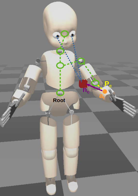
(a) Visual obstacle projected onto the left forearm. The blue lines symbolize the lines of sight of the eyes, not those of the RGB-D camera for simplification.

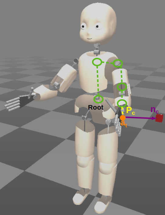
(b) Proximity obstacle mapped to a sensor position on the left hand.

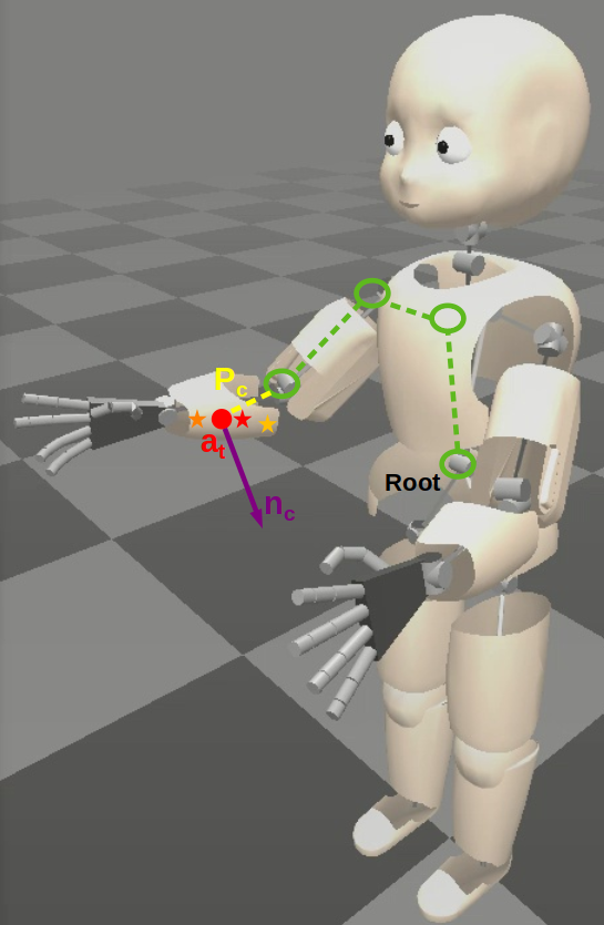
(c) Several tactile stimuli on the right forearm (stars) combined into a super contact $P_{C}$ with a threat level of the highest measured pressure (red color).

Figure 3: Processing of obstacles. Obstacles (red cubes or stars) are projected onto the robot body ($P_{C}$) and connected (yellow line) to the robot kinematic chain (green line). Each collision point is characterized by a normal direction (purple arrow) and threat level (color of the circle, red means highest threat).

The obstacle virtually exists for a specific amount of time with a decreasing threat level imitating that the obstacle is moving away (similar to [9]) to prevent dangerous and jerky movements and to give humans time to react when sensor data are missing or for a post-collision reaction. For example, the threat disappears once the robot moves away from the tactile collision. Without virtual preservation of the obstacle, the robot would return to its original position even when the obstacle is still there.

Visual obstacles in our experiments are human keypoints detected by an RGB-D camera. The method for their detection is based on the work by Docekal et al. [34]. The detected obstacles (see a schematic illustration in Fig. 3(a)) are mapped to parts of the skin where physical contact would eventually occur using PPS projection, similar to [30]. All these mappings are combined into a single position per body part. The collision direction is the vector from the clustered position to the obstacle and the threat level is calculated from their distance.

Proximity sensor data (see a schematic illustration in Fig. 3(b)) are not projected onto the skin taxel, as these sensors are placed to cover parts of the robot without the skin; thus, there is no skin taxel to which information can be projected. However, they are projected onto the sensor position. The threat level is computed from the measured distance, and the collision direction is the direction vector of the sensor beam.

Tactile obstacles (see a schematic illustration in Fig. 3(c)) are processed in the same way as in [17]. Contacts detected by artificial skin sensors (taxels) with a pressure above the threshold value are clustered to super contacts to diminish spiking effects and eliminate false positive detections. The threat level corresponds to the highest measured pressure in the neighborhood, and the collision direction is the normal vector of the central taxel.

II-G Collision avoidance parameters

Obstacle avoidance constraints (Eq. 12) are parameterized by two positive parameters—additive $k_{1}$ and multiplicative $k_{2}$. The parameter $k_{1}$ defines when the maximum approach velocity becomes the minimum repulsive velocity, that is, when $\mathbf{\dot{x}_{a}}$ is lower than zero. The parameter $k_{1}$ has a constant value of 0.3 in our experiments. The parameter $k_{2}$ scales the maximum approach velocity. We found that body links cannot move with the same minimum repulsive velocity due to the kinematic constitution of the robot. The same scale for all parts leads to unfeasible constraints for the upper arm and torso (high value) or small and slow avoidance for the hand and forearm (low value). From our observation, $k_{2}$ should increase from the torso to the hand. In our experiments, $k_{2}$ is 0.06, 0.06, 0.33, 0.53 for the body parts of the torso, upper arm, forearm, and hand, respectively.

II-H Self-collision avoidance

For self-collision avoidance, we sampled each body link to obtain sets of points on the robot surface. These points serve as both virtual obstacles and projected positions on the robot, which are the closest points of the robot to obstacles. Due to the kinematic limitations of our humanoid robot, the projected positions are only on the hand and forearm of the controlled arm(s), and the virtual obstacles are on the common torso and the “primary arm” (hand, forearm, upper arm) when the dual-arm version of the controller is used. The virtual obstacles are not on the secondary arm because of the arm prioritization—only the “secondary arm” avoids the collision with the “primary arm” and not vice versa.

We find the closest pair of virtual obstacles and projected positions for each combination of body parts. If their distance $d_{C}$ is less than a threshold, we add the virtual obstacle to the set of obstacles with a threat level $a_{t}=1-50d_{C}/3$. The collision point is the projected position of the obstacle on the robot ($\mathbf{P}_{C}$), the collision direction ($\mathbf{n}_{C}$) is the vector from the collision point to the virtual obstacle, and the gain ($V_{C}$) is equal to 1.2. Finally, we compute the linear inequality constraint for these obstacles in the same way as for the external obstacles.

II-I Static obstacles

Sometimes, the experiment contains known static objects that the robot should avoid. The almost same procedure as for self-collision avoidance can also be used in this case. Virtual obstacles are sampled from the static object instead of the robot body. The projected positions are points in the robot body parts that can collide with the object. This approach was used, for example, to avoid the table during the interactive game demonstration.

II-J Relative position constraint

In addition to the usual limitations, such as keeping a target pose, we can incorporate another task restriction into the problem as (in-)equality constraints. For the bimanual task experiment, we added one constraint per each axis to keep a specified relative position between the hands (end effectors). The constraint can be written in the vector form as

$$\mathbf{x^{p}}-\mathbf{x^{s}}=\mathbf{d_{\mathrm{rel}}}$$

where $\mathbf{x^{p/s}}$ are the positions of the end effectors, and $\mathbf{d_{\mathrm{rel}}}$ is a relative position vector. This equation can be reformulated for our QP problem with joint velocities as

$$\begin{split}\mathbf{x_{0}^{p}}+\begin{bmatrix}\mathbf{J_{t,pos}^{p}}(\mathbf{q^{t}})&\mathbf{J_{a,pos}^{p}}(\mathbf{q^{p}})\end{bmatrix}\begin{bmatrix}\mathbf{\dot{q}^{t}}\\ \mathbf{\dot{q}^{p}}\end{bmatrix}&-\\ \mathbf{x_{0}^{s}}-\begin{bmatrix}\mathbf{J_{t,pos}^{s}}(\mathbf{q^{t}})&\mathbf{J_{a,pos}^{s}}(\mathbf{q^{s}})\end{bmatrix}\begin{bmatrix}\mathbf{\dot{q}^{t}}\\ \mathbf{\dot{q}^{s}}\end{bmatrix}&=\mathbf{d_{\mathrm{rel}}}\end{split}$$ (14)

where $\mathbf{x_{0}^{p/s}}$ are the current positions of the end effectors, $\mathbf{J^{p/s}_{a,pos}}(\mathbf{q^{p/s}}),\mathbf{J^{p/s}_{t,pos}}(\mathbf{q^{t}})$ are the translational velocity components of the Jacobian matrices for arm and torso, respectively.

II-K Joint position constraints

The joint position bounds for the QP problem have to be set in such a way that the robot joint limits are not exceeded. In our solution, we are inspired by the shaping policy for avoiding joint limits in [4] to maximize reachability in the arm workspace. It consists of a flat region in most of the joint range. Nevertheless, we replaced the original hyperbolic tangent functions by linear and constant functions to fulfill the constraint condition of the QP problem. Since the problem is solved at the velocity level, the joint position limits are expressed using the joint velocities for the joint $i$ as:

$$\dot{q}^{i}_{l}=\dot{q}^{i}_{\mathrm{min}}\cdot c^{i}_{\mathrm{min}},\qquad\dot{q}^{i}_{u}=\dot{q}^{i}_{\mathrm{max}}\cdot c^{i}_{\mathrm{max}}$$

where $\dot{q}^{i}_{\mathrm{min}}$ and $\dot{q}^{i}_{\mathrm{max}}$ are minimum and maximum permissible joint velocity respectively, $c^{i}_{\mathrm{max}}$ and $c^{i}_{\mathrm{min}}$ are obtained from the joint limit avoidance policy as:

$$\begin{split}c^{i}_{\mathrm{min}}&=\begin{cases}0&q^{i}<g_{L}^{i}\\ \frac{q^{i}-g_{L}^{i}}{g_{H}^{i}-g_{L}^{i}}&g_{L}^{i}<=q^{i}<=g_{H}^{i}\\ 1&g_{H}^{i}<q^{i}\end{cases}\\ c^{i}_{\mathrm{max}}&=\begin{cases}0&G_{H}^{i}<q^{i}\\ \frac{q^{i}-G_{H}^{i}}{G_{L}^{i}-G_{H}^{i}}&G_{L}^{i}<=q^{i}<=G_{H}^{i}\\ 1&q^{i}<G_{L}^{i}\end{cases}\end{split}$$ (15)

where $q_{i}$ is a current joint position, $g_{L}^{i}$ and $G_{H}^{i}$ are the lowest and highest permissible joint position value respectively, and $g_{H}^{i}$ and $G_{L}^{i}$ are the thresholds for the joint position constraints.

III Experiments and Results

We prepared seven experiments with a simulated iCub robot and three with a real one to validate the performance of the proposed solution and compare it with other solutions. The experiments overview can be seen in Tab. II.

Exp	Type	Movement	Purpose	Targets	Obstacles
1	Sim	P2P	Reachability	3x3x3 grid	-
2	Sim	P2P	Smoothness	2 poses	-
3	Sim	Circular	Reference tracking	r = 0.08 m	-
4	Sim	Circular	Self-Coll. avoidance	r = 0.1 m	-
5-1	Sim	P2P	Collision avoidance	2 poses	1 with vel. [0, -0.05, 0]
5-2	Sim	P2P	Collision avoidance	2 poses	1 with vel. [0.05, 0, 0]
5-3	Sim	P2P	Collision avoidance	2 poses	1 with vel. [0, 0, -0.05]
11	Real	P2P	Obstacle management	1 pose	multiple obstacles
12	Real	P2P	Obstacle management	2 poses	multiple obstacles
13	Real	Bimanual	Whole solution	1 pose	multiple obstacles

TABLE II: Experiments overview; P2P stands for point-to-point movement.

III-A Experiments in simulation

In simulation, we evaluated the performance of the controller (see Sec. II-B) and the trajectory sampling (see Sec. II-D). The first set of experiments aims to assess reachability, movement smoothness, and reference tracking, without obstacles nearby. Reachability is tested in a reaching experiment (Exp 1) with the targets taken from a grid of 3x3x3 positions in Cartesian space in random order and randomly switched two orientations. The positions are the Cartesian product of $x=$ [-0.23, -0.19, -0.15] m, $y=$ [0.11, 0.15, 0.19] m, $z=$ [0.08, 0.12, 0.16] m, and the orientations are $o_{1}=$ [-0.15, -0.79, 0.59, 3.06], $o_{2}=$ [-0.11, 0.99, 0.02, 3.14] in angle-axis notation. Smooth movement is evaluated in a point-to-point experiment (Exp 2), where the robot moves between two alternating poses $p_{1}=$ [-0.23, 0.26, 0.02, -0.15, -0.79, 0.59, 3.06] and $p_{2}=$ [-0.26, 0.03, 0.03, -0.11, 0.99, 0.01, 3.14], where the first three values are position coordinates in meters and the last four values are the orientation in angle-axis notation. Finally, a circular movement experiment (Exp 3) is chosen to validate the reference tracking. The overview of the experiments can be found in Tab. II.

In addition to the proposed solution, other alternatives and state-of-the-art methods are also evaluated. Specifically, we compare — 1) HARMONIOUS – the proposed solution in the single-arm version; 2) HARMONIOUS2 – the proposed solution in the dual-arm version when the goal of the other arm is to hold a specified position; 3) NEO – the controller by Haviland and Corke [8]; 4) React by Ngyuen et al. [17]; 5) Cart – Cartesian controller for the iCub robot [4], which is evaluated only in Exp 1 and Exp 2 as it primarily serves for point-to-point movements and does not feature avoidance constraints. Controllers 1–4 are evaluated with and without local trajectory sampling (LTS), described in Sec. II-D. Cart has its own local trajectory optimization.

LTS	HARMON	HARMON2	NEO	React	Cart
Yes	91.1 %	90.4 %	77.8 %	86.7 %	90.4 %
No	90.4 %	89.6 %	77.8 %	82.2 %

TABLE III: Reachability experiment (Exp 1). Success rate of combined reachability in position and orientation. LTS stands for local trajectory sampling. Cart has its own local trajectory optimization.

The results for the reachability experiment (Exp 1) are shown in Tab. III. In this experiment, our controller has the highest number of targets that are reached in 6D pose (i.e., position and orientation). The target is reached when the end effector is, at the same time, closer than 5 mm and 0.1 rad to the target. The impact of the local trajectory sampling is visible as all controllers have better (or at least the same) reachability results with sampling than without sampling.

The results of the movement smoothness experiment (Exp 2) show the main impact of the local trajectory sampling (see Fig. 4(a)). Position sampling (Fig. 4(a) left) creates a bell-shaped Cartesian translation velocity profile typical for a human-arm motion [50]. The velocity profile of Cart is the most similar to the exact minimum-jerk movement, as it is specially optimized for it. Other versions are almost identical; only React does not reach zero velocity after 5 s. All versions without local sampling have snap onset and slow jerky decay. Orientation sampling (Fig. 4(a) right) creates a torque-minimal path for the rotation as it travels along the straightest path of the rounded surface of a sphere and it keeps the rotational velocity constant during movement [52], resulting in a visually smooth transition between two rotations. HARMONIOUS and NEO have a smooth angular velocity profile; React velocity profile is not smooth and does not reach zero after 5 s. Cart uses the same sampling for orientation as for position, and thus the resulting angular velocity profile is similar to that for the translational velocity.

In the case of circular movement in the reference tracking experiment (Exp 3), there is no effect of local trajectory sampling, as a new target is generated for each period (the tracked reference), meaning that the smoothness of the movement is handled at a higher level (an external target generator). As shown in Fig. 4(b), HARMONIOUS outperformed others in reference tracking with the lowest position and orientation error.

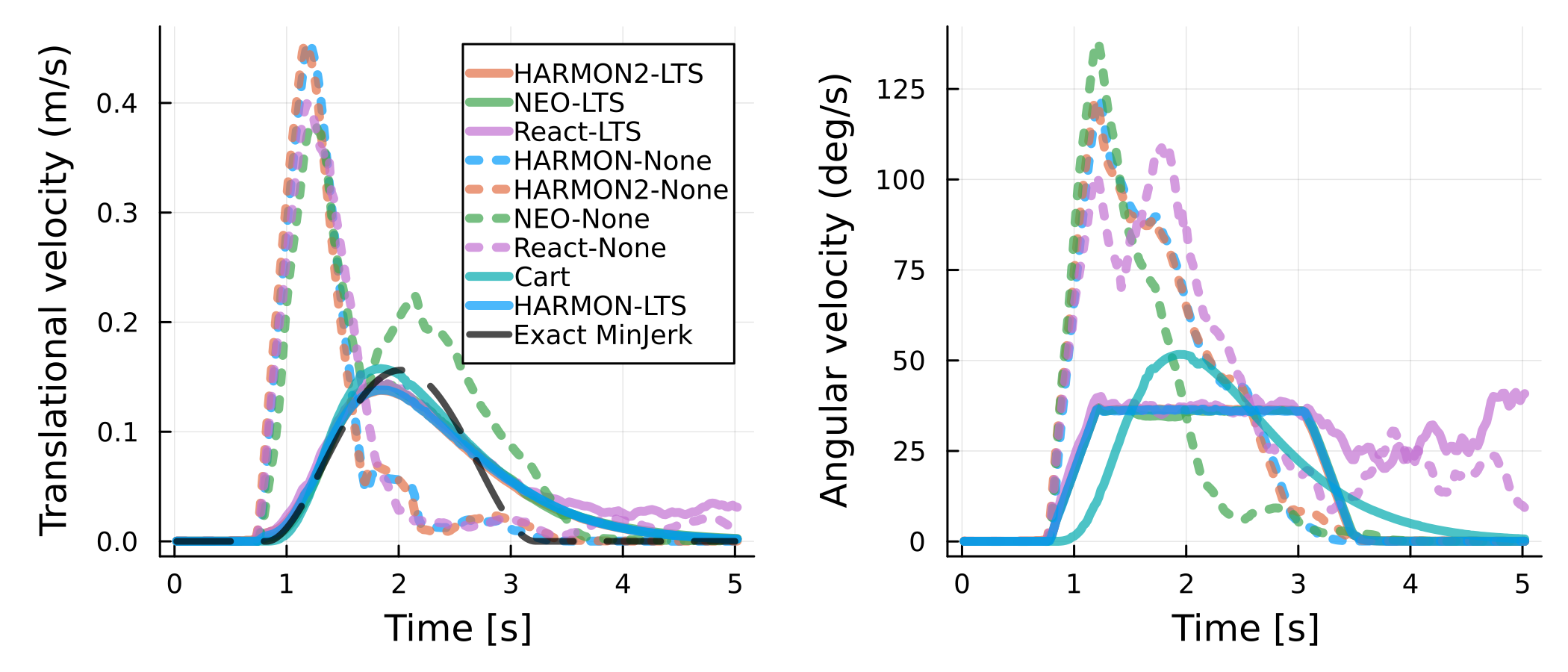
(a) Exp 2: End-effector translational (left) and angular (right) velocity profiles during point-to-point movement and computed exact minimum-jerk translational velocity profile.

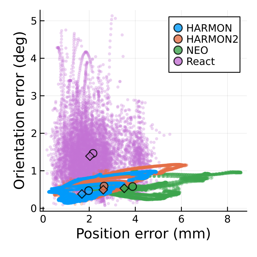
(b) Exp 3: Reference tracking error between desired and actual 6D pose. Circles and diamonds represent mean and median pose error, respectively.

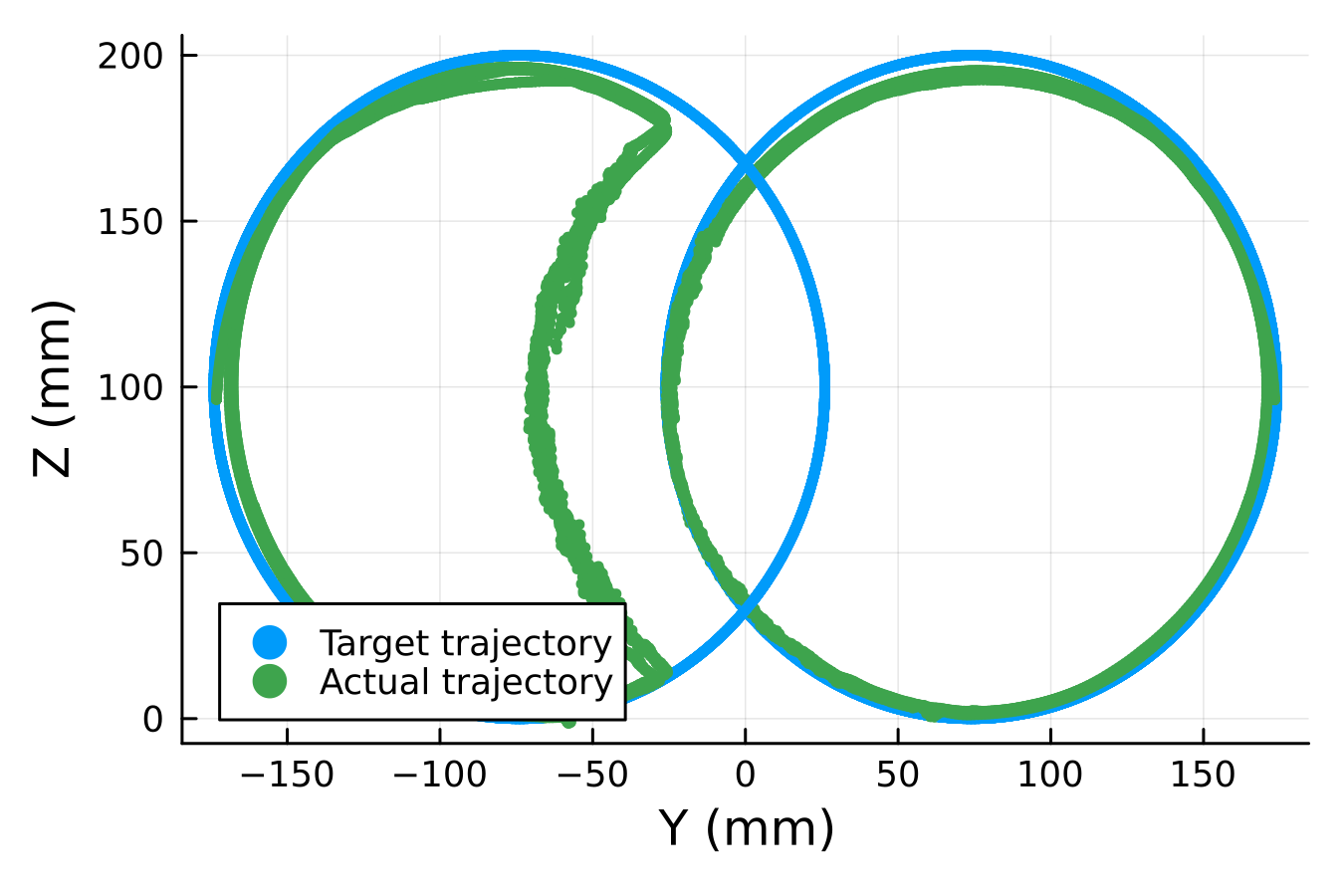
(c) Exp 4: Left and right arms movement for our solution (right set as “primary”).

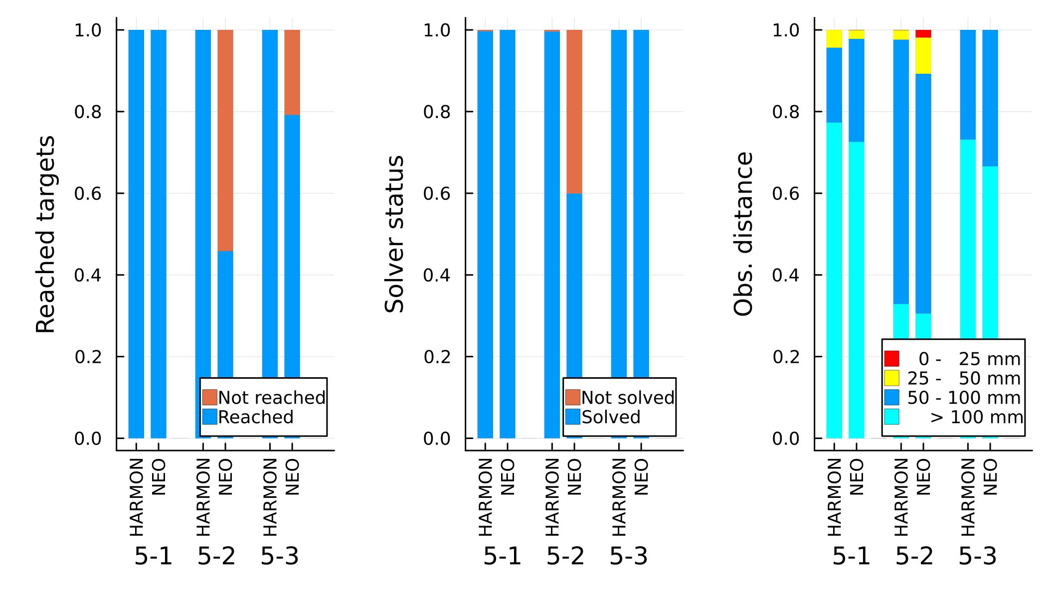
(d) Exp 5: Collision avoidance experiments (Exp 5-1, 5-2, 5-3).

Figure 4: Simulation experiments results. LTS stands for local trajectory sampling.

The next experiment is a circular movement experiment with both arms in opposite directions (Exp 4). It shows how the dual-arm solution works, particularly arm prioritization and self-collision avoidance. As the reference controllers are for single arms only (or separately), only our solution is shown (without trajectory sampling). Figure 4(c) shows the trajectories of both end effectors making circular movements. In this case, the right arm was selected as the “primary arm”. Therefore, the right arm successfully tracks the circle all the time, and the left arm prevents self-collision by keeping a safe distance instead of tracking the circle when the arms are too close.

The last set of simulation experiments tests collision avoidance. For simplicity, the obstacle is virtual and is perceived without noise, omitting the influence of sensor data processing on the results. All three experiments are based on Exp 2 and they differ only in the direction of the obstacle — 1) the obstacle moves along the movement, i.e., in the y-axis direction (Exp 5-1); 2) the obstacle moves towards the robot, i.e., in the x-axis direction (Exp 5-2); 3) the obstacle falls in the z-axis direction (Exp 5-3). In this case, Cart is not included in the comparison because it cannot handle obstacles. React is also omitted because it was outperformed even in experiments without obstacles. Furthermore, more restrictive repulsive vectors were used instead of linear inequality constraints that allow motions in tangential directions. Therefore, we compare only HARMONIOUS and NEO. Figure 4(d) shows the fraction of targets reached during the experiment, the fraction of QP problems successfully solved during the experiments, and the distance between the obstacle and the closest point of the robot, where we assume that a distance of less than 25 mm is too dangerous. There is no significant difference between controllers when the obstacle moves along the robot’s movement (Exp 5-1). On the other hand, the obstacle moving towards the robot (Exp 5-2) is problematic for NEO. Half of the time, the targets are not reached within a time limit and the controller cannot solve the QP problem in almost 40 % runs. Furthermore, the small distances between the robot and the obstacle sometimes lead to collisions. As opposed to NEO, HARMONIOUS has no problem with collisions or reaching in this experiment. Our solution also works adequately in Exp 5-3. NEO did not reach all targets within the time limit, but the distance to an obstacle is safe.

III-B Real robot experiments – collision avoidance

The experiments with the real robot were prepared to evaluate the obstacle processing part of the solution, described in Sec. II-F. We show collision avoidance (visual and proximity modalities) and post-collision reaction (tactile modality) and their combination while the robot keeps position (Exp 11) or moves back and forth between two points as in Exp 2 (Exp 12). When visual obstacles are involved, the iCub gaze controller [53] is employed to point the robot gaze to an appropriate position in the scene, thus compensating for the robot torso joint movements.

Figure 5 graphically illustrates the experiment using snapshots. Figure 6 shows the operation of the main components of HARMONIOUS on plots, focusing on the left arm of the robot (“primary arm” in these experiments). Note that obstacles at or near the robot hand (visual obstacles near the hand or forearm, proximity at the back of the hand, or touch at the hand or forearm) inevitably compromise the task—staying close to the target—whereas visual obstacles or touch at more proximal body parts give the robot the possibility to exploit its kinematic redundancy and fulfill the task while simultaneously avoiding contacts. Parts of Exp 11—robot tasked with keeping the end effector position, while complying with constraints from obstacles spawned by the presence of the human—are shown in Fig. 6(a). In Fig. 6(a) (top), the robot starts in a steady state without obstacles around characterized by a zero target distance (first two seconds, green line). Once a proximity obstacle is detected, the end effector is moving away until the proximity obstacle constraint disappears from the controller and the target position is reached again. Physical contact of the human with the robot hand (around 5 s) and the forearm (around 7 and 9 s) generate constraints and trigger avoidance. Tactile collision with upper arm (12-13 s) and torso (14-15 s) generate avoidance but do not significantly compromise the task, as the robot kinematic redundancy is exploited by the controller.

In Fig. 6(a) (center), the first 10 seconds are very similar to the top one. Touch on the forearm causes deviation from the target while contact with the upper arm is evaded while simultaneously staying close to the target. Touch at the hand (5 s) and proximity signal at the hand (7 s) cause deviation from the target. At around 12 s, a proximity obstacle at the hand is evaded but then avoidance stops as the robot is blocked by contact with the forearm. Once the touch disappears, the proximity collision avoidance continues. Finally, when the proximity obstacle disappears, a tactile stimulus on the hand causes a fast movement towards the target position.

Figure 6(a) (bottom) shows a part of the experiment where, in addition to proximity and tactile obstacles, visual obstacles are spawned by human keypoint detections in the camera input. At first, distant visual stimuli for the torso and hand cause only small end-effector deviations from the target. Then, at 5 s, a physical collision with the torso and upper arm occurred, outside the field of view. In contrast, the subsequent tactile input at the hand (8 s) is also detected by vision. Visual stimuli persist once the collision ends, preventing the robot from reaching the target until they disappear. At the end (12-15 s), we can see the Peripersonal space (PPS) projection to all parts of the skin causing deviation from the target.

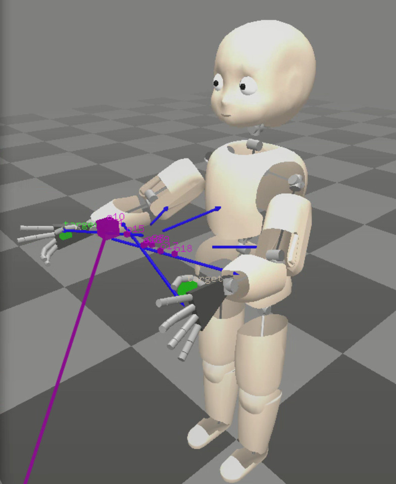
(a) Visualization of visual obstacle avoidance. Green cubes – target positions for the robot end effectors; purple cubes – human keypoints detected, larger cubes for body and smaller for hand keypoints; blue arrows – PPS projections of obstacles onto robot body parts.

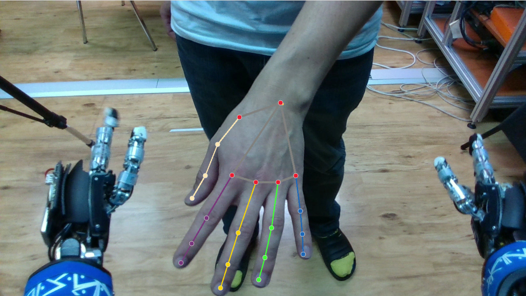
(b) RGB-D camera view of a human approaching the robot with keypoint detections.

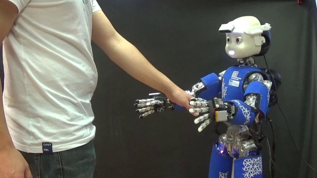
(c) External view – human approaching the robot.

Figure 5: Visualizations from real-world collision avoidance experiments.

In Exp 12, the robot is asked to move between two targets every 9 s. Figure 6(b) show the main system components in action. Figure 6(b) (top) starts with an undisturbed reaching movement to the target, followed by touch on the torso (4 s) and upper arm (6 s) causing only small deviations from the target. To evade contact with the forearm (7 s), distance to target has to increase. In Fig. 6(b) (center), the human physically interferes with the forearm during the approach phase, so the arm has to go around the obstacle to reach the target (2-4 s). After the target is reached, a proximity obstacle pushes the hand away from the target again (6-9 s). The effect of visually detected obstacles is shown in Fig. 6(b) (bottom). At first, visual stimuli block the direct way to the target; thus, the arm goes around the obstacles to prevent collisions (0-4 s). Once the target is reached, new visual obstacles appear (5-7 s), forcing the end effector deviate from the target again. Note that no particular evasive maneuvers to go around an obstacle to the target are built in. Such behaviors are rather emergent from the local behavior of the controller.

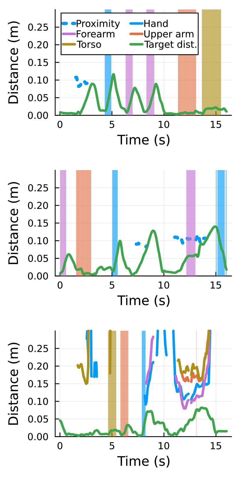
(a) Exp. 11 – Left arm keeping position. Tactile and proximity collision avoidance (top and center), tactile and visual collision avoidance (bottom).

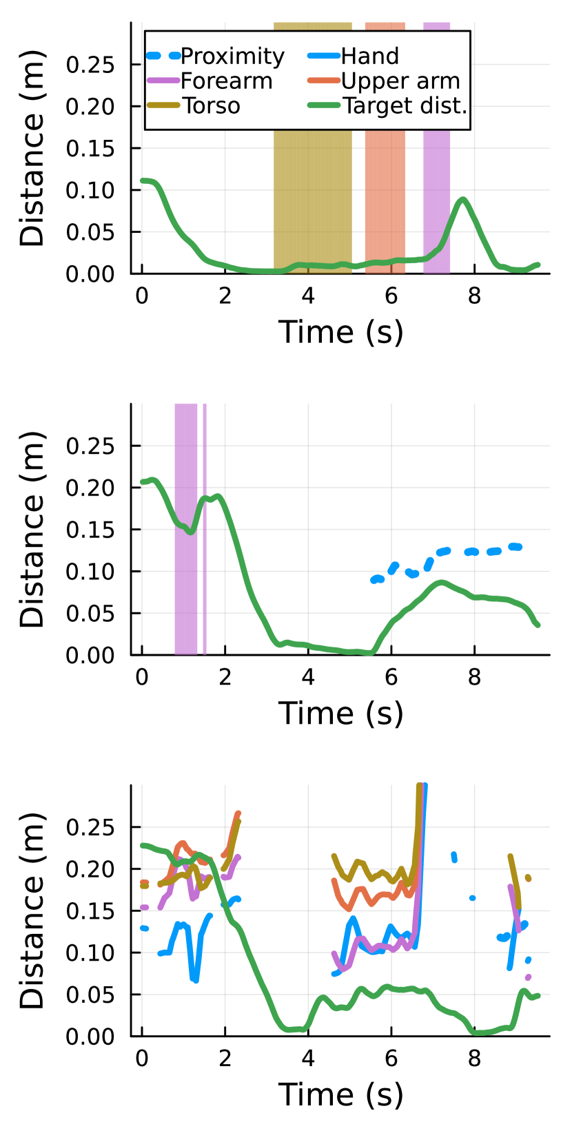
(b) Exp. 12 – Left arm reaching. Tactile collision avoidance (top), proximity and tactile collision avoidance (center), visual collision avoidance (bottom).

Figure 6: Real-world collision avoidance experiments. Green line – distance of end effector (robot hand) to target; solid lines in other colors – distance of visual obstacles to the closest body part; dotted line –- distance to back of robot hand from proximity sensor; vertical lines/stripes –- tactile activations -– contacts with corresponding body parts.

III-C Real robot – bimanual task

We prepared a bimanual task experiment (Exp 13) in which the robot holds a sponge in its hands (see Fig. 7(a)). The target is prescribed for the “primary arm” (left) and an additional constraint is introduced to keep the sponge between the two hands. At the same time, dynamic obstacles spawn additional constraints and avoidance. For this experiment, tactile inputs from the robot hands (palms) are ignored (the robot holds the sponge). This experiment aims to verify that the dual-arm version works and that other task constraints, such as the relative distance vector between the end effectors in this case, can be easily incorporated into the problem definition (the relative position constraint described in Sec. II-J).

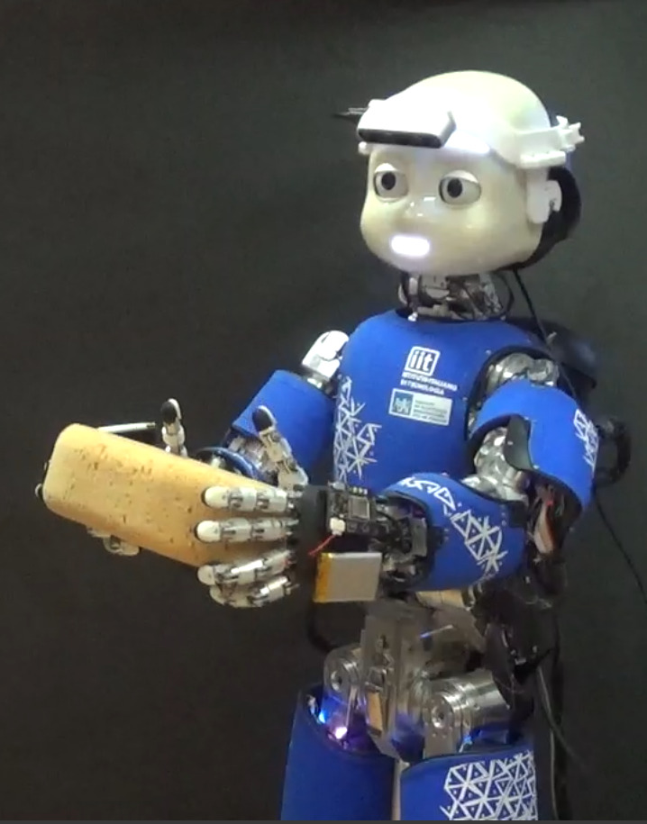
(a) Photo from the experiment.

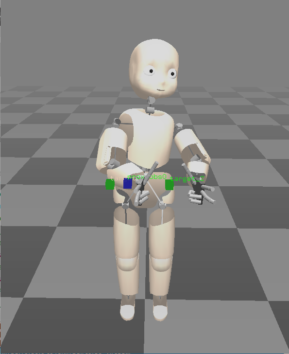
(b) Visualization of hand targets (green cubes) and proximity obstacle (blue cube).

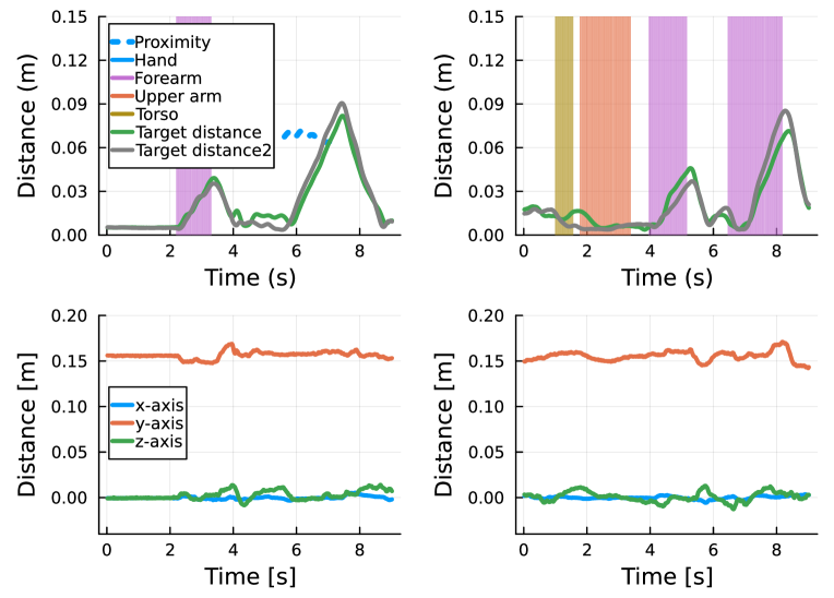
(c) Two sequences from the bimanual task experiment in columns. Obstacle and target distances (top): green and gray lines – distance of end effectors (robot hands) to target; dotted line – distance to back of robot hand from proximity sensor; vertical lines/stripes – tactile activations – contacts with corresponding body parts. Relative position of the end effectors (bottom).

Figure 7: Real robot – bimanual task.

Figure 7(c) shows plots from two sequences of the bimanual task experiment—distances to the target, presence of obstacles for the right and left arms, and the relative position of the end effectors. In the left column, we can see the evasive action of the arms caused by contact with the left forearm and then a proximity obstacle impinging on the left hand. The relative position between both hands remained almost the same as the arms simultaneously moved away from the obstacles, respecting the bimanual constraint. In the right column, we can again see how the high number of degrees of freedom helps to keep the target positions while reacting to contacts on the proximal body parts—torso and upper arm. Contact with the left forearm causes deviation from the target but not losing or squishing the sponge.

Collision avoidance during the bimanual task is more challenging, as it requires a synchronized movement of both arms to keep the specified relative position between them. Therefore, the avoidance movements are smaller compared to previous experiments. The proximity obstacle avoidance is portrayed in Fig. 7(b).

III-D Real robot – Interactive game demonstration

To demonstrate the operation of HARMONIOUS at scale and in a genuine unstructured human-robot interaction scenario, we taught the robot to play a children’s board game called Bubbles. Based on the numbers that appear on the dice and their colors, the players—the robot and the human in our case—compete to pick the card on the table where the size of the colored bubbles corresponds to the colors of the dice, ordered by the numbers – see Fig. 1 and a video at https://youtu.be/gw8JB-1R3bs. This game was chosen because there is a shared physical space with unstructured interaction. The robot processes the visual inputs and recognizes individual cards on the table. After the roll of the dice, the player that first places his hand over the right card wins the round. After choosing the appropriate card, the robot selects which hand to use and initiates the reaching movement. At all times and in real time, visual, proximity and tactile streams are simultaneously processed, spawning obstacles if appropriate and dynamically adding constraints to the robot controller in order to warrant the safety of the human player at all times. The game itself is rather challenging for the human player and hence in order to compete with the robot, he often cheats by pushing the robot physically away or by blocking certain volumes of the workspace by placing his hands over it. This was a deliberate choice to put HARMONIOUS at test.

The controller runs in the dual-arm mode during the game. Depending on the position of the card in every round, the left or right arm is chosen and set as “primary’ (and hence its position reaching target is set as a constraint). Additional constraints were added to the optimization problem by adding static obstacle points (see Sec. II-I) to prevent the robot from colliding with the table. We prepared a high-level Python script to play the game and used the gaze controller [53] to always look at the table. The program loop starts with the processing of rolled dice (numbers sent to the program in the command line) and the current RGB-D image, followed by the detection of cards on the table, the decision of the correct card and computing its 3D position. Then one arm approaches the card position; while the other arm goes to a specific position outside the field of view of the RGB-D camera. After the reach approach (successful or not), the approaching arm returns to a specific position to clear the view for the next round.

The robot with HARMONIOUS running successfully managed to run the game and cope with the unstructured interaction, dynamically processing a large number of obstacles perceived through three different sensory modalities, without endangering the human player.

IV Conclusion, Discussion and Future work

We have developed a real-time reactive motion control system for upper body control of a dual-arm robot with a common torso. The proposed solution (HARMONIOUS) is designed to enable safe and effective interaction with humans in close proximity. In the absence of obstacles, we systematically tested our controller’s reaching ability on a grid of position and orientation targets in the workspace and compared better or at least equally good as alternative controllers, including the one designed specifically for the iCub [4]. We found that assigning different weights to position and orientation tasks is advantageous (unlike in [8]). Preferring arm over torso movements by adjusting weights in the minimization leads to more natural-looking movements. Kinematic singularities are handled through velocity damping and natural kinematic postures are rewarded in the optimization problem formulation. Smooth human-like motions with a bell-shaped Cartesian velocity profile are generated, using biologically inspired local trajectory sampling. Overall, several components act synergestically to produce human-like naturally looking movements.

The full potential of HARMONIOUS lies in the ability to perceive objects in the environment, relate them to the complete surface of the robot body, and, when appropriate, transform them into constraints for the motion controller. We used three sensory modalities: two that sense at a distance, “pre-collision”, vision and proximity, and tactile sensors on large areas of the robot body (2000 individual sensors) providing contact or post-collision information. Information about obstacles from all three modalities—sometimes overlapping, at other times complementary—was processed and transformed into a unified representation dynamically generating constraints for the whole-body motion controller. We have extensively experimentally evaluated HARMONIOUS, compared it to NEO [8] and React [17, 30], demonstrating superior performance. Uniquely to our solution, we commanded both arms and the torso of the iCub humanoid robot (in total 17 DoFs) and demonstrated both the setup where every arm has a separate task and one, set as “primary arm”, commands the torso joints, and a bimanual task where the hands hold an object between them. The performance of HARMONIOUS at scale was finally demonstrated in unstructured physical human-robot interaction while playing a game. Here, additional task constraints were added to the problem formulation.

The solution we presented and its experimental demonstrations are unique in showing the online dynamic incorporation of obstacles perceived through three different sensory modalities and their on the run embedding as whole-body motion constraints into a motion controller with human-like characteristics. At the same time, our solution is by no means restricted to the iCub humanoid robot or to the particular sensory setup. The problem formulation is highly modular and both the minimization criteria (e.g. rewarding natural postures) or constraints to the quadratic program (e.g. obstacles) can be easily removed or different ones added.

Our immediate future work involves adding active gaze control, such that the robot can better perceive what is relevant and, at the same time, reduce the noise in the sensory streams using gaze stabilization, for example.

References

- [1] H. A. Park, M. A. Ali, and C. S. G. Lee, “Closed-form inverse kinematic position solution for humanoid robots,” International Journal of Humanoid Robotics, vol. 9, no. 3, p. 1250022, 2012.
- [2] P. Beeson and B. Ames, “TRAC-IK: An open-source library for improved solving of generic inverse kinematics,” in 2015 IEEE-RAS International Conference on Humanoid Robots, 2015, pp. 928–935.
- [3] S. Lloyd, R. A. Irani, and M. Ahmadi, “Fast and Robust Inverse Kinematics of Serial Robots Using Halley’s Method,” IEEE Transactions on Robotics, vol. 38, no. 5, pp. 2768–2780, Oct. 2022.
- [4] U. Pattacini, F. Nori, L. Natale, G. Metta, and G. Sandini, “An experimental evaluation of a novel minimum-jerk cartesian controller for humanoid robots,” in 2010 IEEE/RSJ International Conference on Intelligent Robots and Systems (IROS), Oct. 2010, pp. 1668–1674.
- [5] K. Glass, R. Colbaugh, D. Lim, and H. Seraji, “Real-Time Collision Avoidance for Redundant Manipulators,” IEEE Transactions on Robotics and Automation, vol. 11, no. 3, pp. 448–457, 1995.
- [6] D. H. Park, H. Hoffmann, P. Pastor, and S. Schaal, “Movement reproduction and obstacle avoidance with dynamic movement primitives and potential fields,” in 2008 IEEE-RAS International Conference on Humanoid Robots, 2008, pp. 91–98.
- [7] F. Flacco, T. Kröger, A. De Luca, and O. Khatib, “A depth space approach to human-robot collision avoidance,” in 2012 IEEE International Conference on Robotics and Automation, 2012, pp. 338–345.
- [8] J. Haviland and P. Corke, “NEO: A novel expeditious optimisation algorithm for reactive motion control of manipulators,” IEEE Robotics and Automation Letters, vol. 6, no. 2, pp. 1043–1050, Apr. 2021.
- [9] C. Escobedo, M. Strong, M. West, A. Aramburu, and A. Roncone, “Contact Anticipation for Physical Human–Robot Interaction with Robotic Manipulators using Onboard Proximity Sensors,” in 2021 IEEE/RSJ International Conference on Intelligent Robots and Systems, Sep. 2021, pp. 7255–7262.
- [10] Y. Ding and U. Thomas, “Collision Avoidance with Proximity Servoing for Redundant Serial Robot Manipulators,” in 2020 IEEE International Conference on Robotics and Automation, May 2020, pp. 10 249–10 255.
- [11] D. Guo and Y. Zhang, “A New Inequality-Based Obstacle-Avoidance MVN Scheme and Its Application to Redundant Robot Manipulators,” IEEE Transactions on Systems, Man, and Cybernetics, Part C (Applications and Reviews), vol. 42, no. 6, pp. 1326–1340, Nov. 2012.
- [12] Y. Tong, J. Liu, X. Zhang, and Z. Ju, “Four-Criterion-Optimization-Based Coordination Motion Control of Dual-Arm Robots,” IEEE Transactions on Cognitive and Developmental Systems, vol. 15, no. 2, pp. 794–807, 2023.
- [13] W. Suleiman, “On inverse kinematics with inequality constraints: New insights into minimum jerk trajectory generation,” Advanced Robotics, vol. 30, no. 17-18, pp. 1164–1172, Sep. 2016.
- [14] D. Rakita, H. Shi, B. Mutlu, and M. Gleicher, “Collisionik: A per-instant pose optimization method for generating robot motions with environment collision avoidance,” in 2021 IEEE International Conference on Robotics and Automation (ICRA), 2021, pp. 9995–10 001.
- [15] O. Khatib, “Real-Time Obstacle Avoidance for Manipulators and Mobile Robots,” Autonomous Robot Vehicles, pp. 396–404, 1986.
- [16] K. Merckaert, B. Convens, C. ju Wu, A. Roncone, M. M. Nicotra, and B. Vanderborght, “Real-time motion control of robotic manipulators for safe human–robot coexistence,” Robotics and Computer-Integrated Manufacturing, vol. 73, p. 102223, Feb. 2022.
- [17] P. D. Nguyen, F. Bottarel, U. Pattacini, M. Hoffmann, L. Natale, and G. Metta, “Merging Physical and Social Interaction for Effective Human-Robot Collaboration,” in 2018 IEEE-RAS International Conference on Humanoid Robots, 2018, pp. 710–717.
- [18] J. Schulman, J. Ho, A. Lee, I. Awwal, H. Bradlow, and P. Abbeel, “Finding Locally Optimal, Collision-Free Trajectories with Sequential Convex Optimization,” in Robotics: Science and Systems IX, 2013, pp. 1–10.
- [19] S. Zimmermann, M. Busenhart, S. Huber, R. Poranne, and S. Coros, “Differentiable Collision Avoidance Using Collision Primitives,” in 2022 IEEE/RSJ International Conference on Intelligent Robots and Systems, Oct. 2022, pp. 8086–8093.
- [20] R. Bordalba, T. Schoels, L. Ros, J. M. Porta, and M. Diehl, “Direct collocation methods for trajectory optimization in constrained robotic systems,” IEEE Transactions on Robotics, vol. 39, no. 1, pp. 183–202, 2023.
- [21] D. E. Whitney, “Resolved Motion Rate Control of Manipulators and Human Prostheses,” IEEE Transactions on Man-Machine Systems, vol. 10, no. 2, pp. 47–53, 1969.
- [22] A. Albini, F. Grella, P. Maiolino, and G. Cannata, “Exploiting Distributed Tactile Sensors to Drive a Robot Arm through Obstacles,” IEEE Robotics and Automation Letters, vol. 6, no. 3, pp. 4361–4368, Jul. 2021.
- [23] A. Cirillo, F. Ficuciello, C. Natale, S. Pirozzi, and L. Villani, “A conformable force/tactile skin for physical human-robot interaction,” IEEE Robotics and Automation Letters, vol. 1, no. 1, pp. 41–48, Jan. 2016.
- [24] E. Magrini and A. De Luca, “Hybrid force/velocity control for physical human-robot collaboration tasks,” in 2016 IEEE International Conference on Intelligent Robots and Systems, Nov. 2016, pp. 857–863.
- [25] N. Mansard, O. Stasse, P. Evrard, and A. Kheddar, “A versatile generalized inverted kinematics implementation for collaborative working humanoid robots: The stack of tasks,” in International Conference on Advanced Robotics (ICAR), June 2009, p. 119.
- [26] C. Escobedo, N. Nechyporenko, S. Kadekodi, and A. Roncone, “A Framework for the Systematic Evaluation of Obstacle Avoidance and Object-Aware Controllers,” in 2022 IEEE/RSJ International Conference on Intelligent Robots and Systems, 2022, pp. 8117–8124.
- [27] Y. Nakamura and H. Hanafusa, “Inverse Kinematic Solutions With Singularity Robustness for Robot Manipulator Control,” Journal of Dynamic Systems, Measurement, and Control, vol. 108, no. 3, pp. 163–171, 09 1986.
- [28] A. Dietrich, T. Wimböck, A. Albu-Schäffer, and G. Hirzinger, “Reactive whole-body control: Dynamic mobile manipulation using a large number of actuated degrees of freedom,” IEEE Robotics and Automation Magazine, vol. 19, no. 2, pp. 20–33, 2012.
- [29] S. Haddadin, H. Urbanek, S. Parusel, D. Burschka, J. Roßmann, A. Albu-Schäffer, and G. Hirzinger, “Real-time reactive motion generation based on variable attractor dynamics and shaped velocities,” in 2010 IEEE/RSJ International Conference on Intelligent Robots and Systems, 2010, pp. 3109–3116.
- [30] D. H. P. Nguyen, M. Hoffmann, A. Roncone, U. Pattacini, and G. Metta, “Compact Real-time Avoidance on a Humanoid Robot for Human-robot Interaction,” in ACM/IEEE International Conference on Human-Robot Interaction, Feb. 2018, pp. 416–424.
- [31] A. Lambert, M. Mukadam, B. Sundaralingam, N. Ratliff, B. Boots, and D. Fox, “Joint Inference of Kinematic and Force Trajectories with Visuo-Tactile Sensing,” in 2019 International Conference on Robotics and Automation, 2019.
- [32] K. He, R. Newbury, T. Tran, J. Haviland, B. Burgess-Limerick, D. Kulić, P. Corke, and A. Cosgun, “Visibility Maximization Controller for Robotic Manipulation,” IEEE Robotics and Automation Letters, vol. 7, no. 3, pp. 8479–8486, Jul. 2022.
- [33] D. Kulić and E. A. Croft, “Real-time safety for human–robot interaction,” Robotics and Autonomous Systems, vol. 54, no. 1, pp. 1–12, Jan. 2006.
- [34] J. Docekal, J. Rozlivek, J. Matas, and M. Hoffmann, “Human keypoint detection for close proximity human-robot interaction,” in 2022 IEEE-RAS 21st International Conference on Humanoid Robots (Humanoids), 2022, pp. 450–457.
- [35] E. Aljalbout, J. Chen, K. Ritt, M. Ulmer, and S. Haddadin, “Learning Vision-based Reactive Policies for Obstacle Avoidance,” in Proceedings of the 2020 Conference on Robot Learning. PMLR, 2020, pp. 2040–2054.
- [36] S. Haddadin, A. De Luca, and A. Albu-Schäffer, “Robot collisions: A survey on detection, isolation, and identification,” IEEE Transactions on Robotics, vol. 33, no. 6, pp. 1292 – 1312, 2017.
- [37] R. Calandra, S. Ivaldi, M. P. Deisenroth, and J. Peters, “Learning torque control in presence of contacts using tactile sensing from robot skin,” in 2015 IEEE-RAS International Conference on Humanoid Robots, 2015, pp. 690–695.
- [38] A. Albini, S. Denei, and G. Cannata, “Enabling natural human-robot physical interaction using a robotic skin feedback and a prioritized tasks robot control architecture,” in 2017 IEEE-RAS International Conference on Humanoid Robots, 2017, pp. 99–106.
- [39] J. Kuehn and S. Haddadin, “An Artificial Robot Nervous System to Teach Robots How to Feel Pain and Reflexively React to Potentially Damaging Contacts,” IEEE Robotics and Automation Letters, vol. 2, no. 1, pp. 72–79, Jan. 2017.
- [40] P. Svarny, J. Rozlivek, L. Rustler, M. Sramek, Özgür Deli, M. Zillich, and M. Hoffmann, “Effect of active and passive protective soft skins on collision forces in human–robot collaboration,” Robotics and Computer-Integrated Manufacturing, vol. 78, p. 102363, 2022.
- [41] F. Flacco and A. De Luca, “Real-time computation of distance to dynamic obstacles with multiple depth sensors,” IEEE Robotics and Automation Letters, vol. 2, no. 1, pp. 56–63, 2016.
- [42] S. Mühlbacher-Karrer, M. Brandstötter, D. Schett, and H. Zangl, “Contactless Control of a Kinematically Redundant Serial Manipulator Using Tomographic Sensors,” IEEE Robotics and Automation Letters, vol. 2, no. 2, pp. 562–569, Apr. 2017.
- [43] A. Roncone, M. Hoffmann, U. Pattacini, L. Fadiga, and G. Metta, “Peripersonal Space and Margin of Safety around the Body: Learning Visuo-Tactile Associations in a Humanoid Robot with Artificial Skin,” PLOS ONE, vol. 11, no. 10, pp. 1–32, 10 2016.
- [44] J. Cléry and S. B. Hamed, “Frontier of self and impact prediction,” Frontiers in psychology, vol. 9, p. 1073, 2018.
- [45] A. Roncone, M. Hoffmann, U. Pattacini, and G. Metta, “Learning peripersonal space representation through artificial skin for avoidance and reaching with whole body surface,” in 2015 IEEE/RSJ International Conference on Intelligent Robots and Systems (IROS), 2015, pp. 3366–3373.
- [46] G. Metta, L. Natale, F. Nori, G. Sandini, D. Vernon, L. Fadiga, C. von Hofsten, K. Rosander, M. Lopes, J. Santos-Victor, A. Bernardino, and L. Montesano, “The iCub humanoid robot: An open-systems platform for research in cognitive development,” Neural Networks, vol. 23, no. 8, pp. 1125–1134, 2010.
- [47] P. Maiolino, M. Maggiali, G. Cannata, G. Metta, and L. Natale, “A flexible and robust large scale capacitive tactile system for robots,” IEEE Sensors Journal, vol. 13, no. 10, pp. 3910–3917, 2013.
- [48] C. Escobedo and M. Strong, “HIRO Skin Unit,” https://github.com/HIRO-group/skin_unit_setup, 2020.
- [49] T. Yoshikawa, “Manipulability of robotic mechanisms,” The International Journal of Robotics Research, vol. 4, no. 2, pp. 3–9, 1985.
- [50] T. Flash and N. Hogan, “The coordination of arm movements: an experimentally confirmed mathematical model,” Journal of Neuroscience, vol. 5, no. 7, pp. 1688–1703, 1985.
- [51] R. Shadmehr and S. Wise, “Supplementary documents for “computational neurobiology of reaching and pointing”,” https://storage.googleapis.com/wzukusers/user-31382847/documents/5a7253343814f4Iv6Hnt/minimumjerk.pdf, 2005, accessed: October 13, 2023.
- [52] K. Shoemake, “Animating rotation with quaternion curves,” SIGGRAPH Comput. Graph., vol. 19, no. 3, p. 245–254, jul 1985.
- [53] A. Roncone, U. Pattacini, G. Metta, and L. Natale, “A Cartesian 6-DoF Gaze Controller for Humanoid Robots,” in Proceedings of Robotics: Science and Systems, AnnArbor, Michigan, June 2016.