Seg2Reg: Differentiable 2D Segmentation to 1D Regression Rendering for 360 Room Layout Reconstruction

Abstract

State-of-the-art single-view 360${}^{\circ}\,$room layout reconstruction methods formulate the problem as a high-level 1D (per-column) regression task. On the other hand, traditional low-level 2D layout segmentation is simpler to learn and can represent occluded regions, but it requires complex post-processing for the targeting layout polygon and sacrifices accuracy. We present Seg2Reg to render 1D layout depth regression from the 2D segmentation map in a differentiable and occlusion-aware way, marrying the merits of both sides. Specifically, our model predicts floor-plan density for the input equirectangular 360${}^{\circ}\,$image. Formulating the 2D layout representation as a density field enables us to employ ‘flattened’ volume rendering to form 1D layout depth regression. In addition, we propose a novel 3D warping augmentation on layout to improve generalization. Finally, we re-implement recent room layout reconstruction methods into our codebase for benchmarking and explore modern backbones and training techniques to serve as the strong baseline. Our model significantly outperforms previous arts. The code will be made available upon publication.

1 Introduction

Room layout estimation is one of the fundamental vision problems toward scene understanding. The goal is to reconstruct the outermost room structure, usually comprising the floor, ceiling, walls, and sometimes columns and beams. Room layout is crucial in various indoor tasks, such as holistic 3D reconstruction [51, 22, 49, 47], image synthesis [43, 10], floor-plan estimation [4, 34], and extreme baseline SfM [33, 14]. Automatic layout annotation for panoramas is also a sought-after feature in real estate portals.

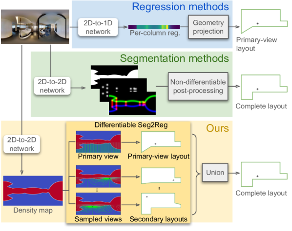
Figure 1: Regression methods directly predict layout geometry. A powerful 2D-to-1D decoder is essential to capture high-level cues within an image column. The regressed layout pertains solely to the visible region from the camera origin (dubbed primary-view layout). Segmentation methods predict lower-level per-pixel probabilities of layout facades, corners, and boundaries. While capable of modeling occluded regions, they require a non-differentiable post-heuristic to convert segmentation to layout geometry. Our proposed Seg2Reg aims to synergize the strengths of both. We re-formulate 2D layout representation as 2D density field via projecting pixels onto the floor or ceiling. We use the classical volume rendering technique to render depth on the density map, which is differentiable and occlusion-aware. The 1D depth maps rendered from the primary view and the sampled secondary views directly outline the layout polygons.

Traditional deep-learning methods view room-layout estimation as semantic segmentation tasks for perspective images [52, 15, 21] or panoramas [54, 45, 31, 55]. The downside of previous segmentation-based methods is that they need heuristic post-processing steps, which introduce errors and gaps between the training objective and the targeted layout outcomes. Recent advancements in 360${}^{\circ}\,$room-layout estimation involve training deep models to regress the boundary [35, 36] or distance to layout wall [39, 18] for each image column (i.e., 1D regression). The regressed geometry information can then be directly projected onto the floor to form a layout floor-plan polygon. Despite achieving state-of-the-art accuracy, regression-based methods require a robust and large decoder to learn to capture global-scale information. Moreover, these methods still rely on post-processing heuristics to infer occluded regions.

Our method, Seg2Reg, enables the differentiable rendering of 1D layout depth (i.e., distance to wall) to form floor-plan polygon from 2D segmentation-based representation on a 360${}^{\circ}\,$image (Fig. 1). The key insight is to re-formulate the 2D layout representation as 2D floor-plan density field, allowing us to employ the classical volume rendering technique [19, 26], which has recently gained great success in 3D NeRF [27] modeling, to compute geometry information in a soft and differentiable manner. Like NeRF, our method involves volume rendering of rays, but in our case, the ‘ray’ trajectory is on the predicted 2D density logit map rather than in 3D space, and the ray should be bent as per the 360${}^{\circ}\,$imaging.

Notably, we show that it is crucial to train our segmentation-based representation with the regression objective, which aligns more directly with our intended task goals. Solely training with the segmentation objective results in lower accuracy, suggesting that our Seg2Reg is the missing piece in earlier segmentation-based methods [54, 45, 31, 55] to achieve state-of-the-art performance. Beyond the visible layout, the volume rendering algorithm and our predicted density map are occlusion-aware, so we can also directly render the floor-plan polygon vertices for the occluded region.

Our codebase, dubbed PanoLayoutStudio, implements various modern backbones and training techniques. Additionally, we extend the widely-used PanoStretch [35] data augmentation to allow for more flexible random adjustments on layout corners. Finally, we reproduce most of the recent methods in our codebase, establishing a stronger baseline for fair comparisons and providing a resource for future works to reuse or recombine various components.

In summary, our contributions are as follows: i) The proposed Seg2Reg differentiably renders 1D regression from 2D segmentation, marrying the merits of both formulations and resulting in a smaller yet stronger model. ii) Our method directly estimates occluded layouts without relying on heuristic post-processing. iii) We introduce a new data-augmentation scheme that allows for flexible layout 3D adjustments. iv) We make a system-level contribution by modernizing the backbones and the training recipes for layout estimation and reproducing previous methods in our codebase—PanoLayoutStudio, which boosts all methods and eases future efforts with reusable modules.

2 Related work

Panorama layout estimation.

Early layout estimation takes perspective images as input [52, 15, 21], while recent approaches increasingly focus on panoramic images and often rely on predicting distinct scene structures, such as ceiling, floor boundaries, or wall corners [51, 54, 35, 36, 55, 8]. LayoutNet [54] is the first to predict boundaries and corners on a single panoramic image using deep neural networks.

HorizonNet [35] is the pioneering method to reformulate this task as a per-column regression problem, utilizing a powerful deep model to regress boundary positions instead of the conventional low-level heatmap layout encoding. Succeeding enhancements are made from both the model architecture [36] and the layout representation [39]. LGTNet [18] takes a step further by employing a transformer-based architecture with an improved layout formulation, which consists of layout depth and layout height, ultimately achieving state-of-the-art quality.

Since LayoutNet [54], segmentation-based works also seek to boost quality by improving layout encoding [45] and network architecture [31, 55]. In contrast to regression-based methods, where model predictions can be directly projected into 3D, segmentation-based methods heavily depend on post-heuristic to convert heatmap predictions into layout geometry. We find that the disconnection between the training objective and the final outcome is a bottleneck in achieving superior results, and we propose to reformulate the probability heatmap as a 2D density field so that we can employ differentiable rendering for the geometric regression properties as well.

Neural radiance field.

NeRF [27] is the de facto method for multiview 3D reconstruction research in recent years. It combines MLP and volume rendering [19, 26] to model the density field and color field of a scene. Subsequent works [37, 9, 28, 3] show that MLP is not necessary while some grid-based representations can also work well. Inspired by their success, we train an ultra-light model to predict a low-level 2D density field and leverage volume rendering to accumulate density into high-level geometric properties, forming 2D polygons directly and differentiably.

Data augmentation.

The progress of data augmentations for perspective images [50, 48, 7, 5, 23, 6, 12, 53] is rapid in recent years as it plays a crucial role in achieving better results. Among these augmentations, geometric-based data augmentation is found to be especially beneficial [6]. Unfortunately, geometric-based data augmentation for 360${}^{\circ}\,$layout estimation is rather limited. PanoStretch [35] randomly adjusts layout aspect ratio. PanoMixSwap [13] uses a generative model to mix furniture, backgrounds, and layout structures from different 360${}^{\circ}\,$images, which is, however, time-consuming. The challenge is that existing geometric augmentation, such as image y-translation, breaks the underlying ground-truth layout sanity, which makes them inapplicable. We present a principled solution to perform geometric data augmentation for 360${}^{\circ}\,$layout, enabling the generation of a more diverse data distribution beyond existing techniques.

3 Approach

The input is a 360${}^{\circ}\,$panoramic image $\mathcal{I}\in\mathbb{R}^{H\times W\times 3}$ under equirectangular projection. The target room layout can be represented by a sequence of 2D coordinates $\{\mathbf{v}_{i}^{*}\}_{i=1}^{K}$, which forms a $K$-edge polygon outlining the floor plan, with a scalar $0pt^{*}$ for the layout height. To fix the scale ambiguity, we follow the literature to rescale the camera-to-floor distance to $1.6$ meters. In Sec. 3.1, we introduce our novel layout representation and floor-plan polygon rendering. Sec. 3.2 details our model design. Sec. 3.3 presents a new principle to perform geometric augmentation for 360${}^{\circ}\,$layout tasks. Finally, Sec. 3.4 presents our codebase.

3.1 Seg2Reg

Our layout representation is a pixel-level density logit map $\widetilde{\mathcal{D}}\in\mathbb{R}^{H\times W\times 1}$. We can use $\mathrm{Softplus}$ to convert the density logit into non-negative density:

$$\mathcal{D}=\log\left(1+\exp\left(\widetilde{\mathcal{D}}\right)\right)~{}.$$ (1)

When projected to the floor or ceiling, the density $\mathcal{D}_{q}$ indicates a pixel $q$ is exterior (i.e., high density) or interior (i.e., low density) to the room layout. Unlike segmenting layout walls, the density map needs to ‘see through’ walls that might be blocking the view for an interior region (Fig. 2).

Overview.

We set the floor plane position at $z^{\mathrm{(floor)}}{=}1.6$ and a temporary ceiling plane position at $z^{\mathrm{(ceiling)}}{=}{-}1$ (we use z-down positive world coordinate system). The upper- and bottom-half of $\mathcal{D}$ (i.e., first and last $\frac{H}{2}$ image rows) estimate the density on the ceiling and floor planes, respectively. In the following, we introduce our algorithm to render the 2D layout polygon on the floor plane. The same algorithm can be applied to render the ceiling-projected polygon. Following standard practice [35, 36, 39], we take the polygon on the floor as the main 2D layout outline, while the ceiling polygon is only used to infer the layout height $0pt$.

‘Flattened’ volume rendering on the 2D floor plan.

We illustrate the rendering of a ray in Fig. 3. Given a camera position $\mathbf{r}_{\mathrm{o}}$ and a unit vector of the ray direction $\mathbf{r}_{\mathrm{d}}$ on the 2D layout of the floor plan, we want to render the expected distance $d$ to the layout exterior based on the estimated $\widetilde{\mathcal{D}}$. We first sample a series of $K$ points on the ray, denoted by $\{\mathbf{r}_{\mathrm{o}}+t_{i}\mathbf{r}_{\mathrm{d}}\}_{i=1}^{K}$, ordered from nearest to farthest. The opacity $\alpha_{i}\in[0,1]$ of the $i$-th sampled point is

$$\alpha_{i} =1-\exp\left(-\rho_{i}\Delta_{i}\right)~{},$$ (2a)

$$\rho_{i} =\mathrm{Softplus}(\tilde{\rho}_{i})~{},$$ (2b)

$$\tilde{\rho}_{i} =\mathrm{Interp}\left(\mathbf{u}_{i},\widetilde{\mathcal{D}}\right)~{},$$ (2c)

$$\mathbf{u}_{i} =\mathrm{EqProj}\left(\left[\mathbf{r}_{\mathrm{o}}+t_{i}\mathbf{r}_{\mathrm{d}},z^{\mathrm{(floor)}}\right]\right)~{},$$ (2d)

where $\mathrm{EqProj}(\cdot)$ projects the 3D point to equirectangular image coordinate $\mathbf{u}$, $\mathrm{Interp}(\mathbf{u},\widetilde{\mathcal{D}})$ bilinearly interpolates the density $\rho$ of point $\mathbf{u}$ on $\widetilde{\mathcal{D}}$, and $\Delta_{i}$ is the spherical distance of the $i$-th ray segment projected to a unit sphere. Please refer to the supplementary for the details of the coordinate system and transformation in this work. We apply the $\mathrm{Softplus}$ activation after the interpolation (post-activation) for sharper decision boundary [37]. Finally, the distance to layout boundary $d$ is computed by alpha blending:

$$d=\sum\nolimits_{i=1}^{K}T_{i}\alpha_{i}t_{i}~{},\text{where}~{}T_{i}=\prod\nolimits_{j=1}^{i-1}\left(1-\alpha_{j}\right)~{}.$$ (3)

The differentiable term $(T_{i}\alpha_{i})$ is the probability of the ray stopping at point $(\mathbf{r}_{\mathrm{o}}+t_{i}\mathbf{r}_{\mathrm{d}})$. Hereinafter, we use

$$\mathrm{Hit}(\mathbf{r}_{\mathrm{o}},\mathbf{r}_{\mathrm{d}}){=}\mathbf{r}_{\mathrm{o}}+d\mathbf{r}_{\mathrm{d}}$$ (4)

to denote the expected ray-polygon intersection by rendering depth. The dependent density logit map $\widetilde{\mathcal{D}}$ and the plane position $z$ of the function are omitted for brevity.

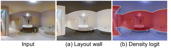
Figure 2: Layout wall vs. our density logit. (a) Layout wall segmentation delineates the room layout in the image space. (b) We train the model to predict a pixel density map when projected to the floor or ceiling planes. The density map enables us to render depth in a soft and differentiable way (Sec. 3.1).

\begin{overpic}[trim=0.0pt 321.2pt 411.53749pt 0.0pt,clip,width=433.62pt,clip]{figs/volrend.pdf} \put(20.0,220.0){\footnotesize$\mathbf{r}_{\mathrm{o}}$} \put(250.0,250.0){\footnotesize$\mathbf{r}_{\mathrm{o}}+t_{i}\mathbf{r}_{\mathrm{d}}$} \par\put(600.0,238.0){\footnotesize$\mathrm{EqProj}$ (\lx@cref{creftype~refnum}{subeq:eqproj})} \put(600.0,125.0){\footnotesize\lx@cref{creftype~refnum}{eq:alpha}} \put(280.0,150.0){\footnotesize$\alpha_{i}$} \par\put(12.0,140.0){\footnotesize$\alpha$} \put(12.0,75.0){\footnotesize$T$} \par\put(10.0,18.0){\scriptsize Alpha blending (\lx@cref{creftype~refnum}{eq:alpha_blending}) for layout depth} \end{overpic}

Figure 3: Visualization of the ‘flattened’ volume rendering from a given ray. Please refer to Sec. 3.1 for the details.

Primary layout polygon.

With the flattened volume rendering algorithm, we can now directly render an $M$-edge polygon from a given camera center $\mathbf{r}_{\mathrm{o}}$:

$$\mathrm{RendPoly}_{M}\left(\mathbf{r}_{\mathrm{o}}\right)=\left\{\mathrm{Hit}\left(\mathbf{r}_{\mathrm{o}},~{}\mathbf{r}_{\mathrm{d}}^{(M)}[i]\right)\right\}_{i=1}^{M}~{},$$ (5)

where $\mathbf{r}_{\mathrm{d}}^{(M)}$ is a set of $M$ unit-vectors uniformly spacing around a circle. We synthesize a $W$-edge primary polygon by placing a camera at $(0,0)$:

$$\left\{\mathbf{v}^{\mathrm{(primary)}}_{i}\right\}_{i=1}^{W}=\mathrm{RendPoly}_{W}\left((0,0)\right)~{},$$ (6)

so the distance to each of the $W$ vertices corresponds to the layout depth of the source image column. In case of no self-occlusion, the rendered primary layout polygon is capable of representing the whole room. We illustrate the layout polygon rendering in Fig. 4.

Secondary layout polygons.

To inference the occlusion region, we sample additional cameras $\mathbf{r}_{\mathrm{o}}^{\prime}$ from the interior region to render a set of $N^{\mathrm{(secondary)}}$ layout polygons

$$\{\mathrm{RendPoly}_{W}\left(\mathbf{r}_{\mathrm{o}}^{\prime}[i]\right)\}_{i=1}^{N^{\mathrm{(secondary)}}}~{}.$$ (7)

The interior region is determined from the primary layout polygon during testing, while we sample from the ground-truth interior region during training. We can compute the union over polygons to merge the secondary polygons into the primary ones. We also implement a rendering noise (due to numerical integration) robust algorithm based on minimum spanning tree and tree diameter, which is detailed in the supplementary material.

\begin{overpic}[trim=0.0pt 281.04999pt 331.23749pt 0.0pt,clip,width=433.62pt,clip]{figs/rendpoly.pdf} \put(175.0,287.0){\footnotesize\lx@cref{creftype~refnum}{eq:poly_primary}} \put(730.0,287.0){\footnotesize\lx@cref{creftype~refnum}{eq:poly_2nd}} \par\put(40.0,240.0){\scriptsize$\mathrm{RendPoly}\left((0,0)\right)$} \put(385.0,240.0){\scriptsize$\mathrm{RendPoly}\left(\mathbf{r}_{\mathrm{o}}^{\prime}[1]\right)$} \put(730.0,240.0){\scriptsize$\mathrm{RendPoly}\left(\mathbf{r}_{\mathrm{o}}^{\prime}[N]\right)$} \end{overpic}

Figure 4: Primary and secondary layout polygons rendering. Our model predicts the density logit (Eq. 1). Given a camera position $\mathbf{r}_{\mathrm{o}}$ on the floor plan, we employ ‘flattened’ volume rendering (Eqs. 2 and 3) to render a layout polygon, $\mathrm{RendPoly}\left(\mathbf{r}_{\mathrm{o}}\right)$, based on the predicted density logit map.

Layout height inference.

The value of $z^{\mathrm{(floor)}}$ is fixed, so we only have to estimate the ceiling plane’s $z$ position. First, the ceiling polygon $\{\mathbf{v}^{\mathrm{(ceiling)}}\}_{i=1}^{W}$ is rendered in the same way as the floor in Eq. 6 but on the temporary ceiling plane position $z^{\mathrm{(ceiling)}}$ instead. We then find the scale

$$s^{*}=\min_{s}\sum_{i=1}^{W}\left(\left\|\mathbf{v}^{\mathrm{(primary)}}_{i}\right\|-s\left\|\mathbf{v}^{\mathrm{(ceiling)}}_{i}\right\|\right)^{2}$$ (8)

that aligns the ceiling polygon to the primary floor polygon. The formula of the layout height by solving least-squares is

$$h=z^{\mathrm{(floor)}}-z^{\mathrm{(ceiling)}}\frac{\sum_{i=1}^{W}\left\|\mathbf{v}^{\mathrm{(primary)}}_{i}\right\|\left\|\mathbf{v}^{\mathrm{(ceiling)}}_{i}\right\|}{\sum_{i=1}^{W}\left\|\mathbf{v}^{\mathrm{(ceiling)}}_{i}\right\|^{2}}~{}.$$ (9)

Relation to binary segmentation.

We can merge the Eqs. 2a and 2b as

$$\begin{split}\alpha&=1-\exp\left(-\mathrm{Softplus}(\tilde{\rho})\Delta\right)\\ &=1-\exp\left(-\log\left(1+\exp\left(\tilde{\rho}\right)\right)\Delta\right)\\ &=1-\left(1+\exp\left(\tilde{\rho}\right)\right)^{-\Delta}\\ &=1-\mathrm{Sigmoid}\left(-\tilde{\rho}\right)^{\Delta}~{},\end{split}$$ (10)

where the subscripts are omitted for brevity. The spherical distance of a pixel height on the equirectangular image is $\frac{\pi}{H}$. We re-scale $\Delta$ by $\frac{H}{\pi}$ so the opacity of a vertical ray segment centered at a pixel $q$ can be simplified to

$$\alpha_{q}=1-\mathrm{Sigmoid}\left(-\widetilde{\mathcal{D}}_{q}\right)=\mathrm{Sigmoid}\left(\widetilde{\mathcal{D}}_{q}\right)~{}.$$ (11)

We can see that the predicted density logit map $\widetilde{\mathcal{D}}$ can be reduced to the binary segmentation logit if we do not apply rendering, which enables us to apply segmentation loss as a training auxiliary.

Training objective.

For each ray to render the primary and secondary layout polygons, we also compute their depth to the ground-truth polygon. Minimizing the difference between the rendered and ground-truth depth directly introduces ambiguity, as there exists an infinite number of weight distributions in the alpha blending (Eq. 3) that can yield the same result. Instead, we derive a compact weight distribution $w^{*}$ that renders the ground-truth depth with only the two nearest points having weight (detailed in the supplementary). We directly guide the alpha blending weight distribution of a ray in Eq. 3 via cross-entropy loss:

$$-w^{*}_{K+1}\log\left(T_{K+1}\right)-\sum\nolimits_{i=1}^{K}w^{*}_{i}\log\left(T_{i}\alpha_{i}\right)~{}.$$ (12)

We apply the cross-entropy loss to the rendered primary and secondary layouts, and the losses are denoted as $\mathcal{L}^{\mathrm{(pri.)}}$ and $\mathcal{L}^{\mathrm{(2nd)}}$, respectively. The cross-entropy loss for the alpha blending weight mainly focuses on the interior and boundary regions. To prevent random results in the far exterior region, we also apply binary segmentation loss $\mathcal{L}^{\mathrm{(seg.)}}$ to the predicted density logit. Our final training objective is

$$\mathcal{L}=w_{1}\,\mathcal{L}^{\mathrm{(pri.)}}+w_{2}\,\mathcal{L}^{\mathrm{(2nd)}}+w_{3}\,\mathcal{L}^{\mathrm{(seg.)}}~{}.$$ (13)

3.2 Network architecture

We first detail our network architecture for predicting the density logit map and then compare our approach with closely related work.

Backbone.

The backbone predicts a feature pyramid in four levels for the input image:

$$\{\mathcal{F}_{i}\in\mathbb{R}^{H_{i}\times W_{i}\times C_{i}}\}_{i=1}^{4}=\mathrm{Enc}(\mathcal{I})~{},$$ (14)

where $H_{i}{=}\frac{H}{2^{i+1}}$, $W_{i}{=}\frac{W}{2^{i+1}}$, and $C_{i}$ is the backbone’s channel dimension.

Segmentation-based 2D decoder.

We adopt an all-MLP decoder design [42] to predict density logit map:

$$\hat{\mathcal{F}}_{i} =\mathrm{Upsample}_{(H,W)}\left(\mathrm{Linear}_{C_{i}\rightarrow D}(\mathcal{F}_{i})\right)~{},$$ (15a)

$$\widetilde{\mathcal{D}} =\mathrm{Linear}_{D\rightarrow 1}\left(\mathrm{GELU}\left(\sum\nolimits_{i=1}^{4}\hat{\mathcal{F}}_{i}\right)\right)~{},$$ (15b)

where $\mathrm{Linear}_{C_{i}\rightarrow C_{o}}(\cdot)$ is a linear layer mapping the number of latent channels from $C_{i}$ to $C_{o}$, and $\mathrm{Upsample}_{(H,W)}(\cdot)$ bilinearly interpolates the spatial size to $(H,W)$.

Discussions about top-down view models.

Our Seg2Reg can also be applied to top-down view (i.e., ceiling view, floor-plan view, or bird’s-eye view) segmentation-based models [45, 31]. However, we find it hard to choose an appropriate perspective field-of-view as small FoVs miss farther walls while large FoVs limit the space for closer regions. We mainly follow recent state-of-the-art to use equirectangular view and leave our method’s application to perspective view for potential future explorations.

3.3 Layout 3D warping

A recent finding [6] suggests that geometric transformations are especially helpful in improving model generalizability among various data augmentations. Unfortunately, many commonly used perspective image transformations do not apply to 360${}^{\circ}\,$layout estimation. For instance, when we apply image y-translation (Fig. 5’s (b)), the projected polygons of ceiling and floor boundaries get distorted and do not match in shape, while we rely on their alignment scaling factor to compute the ground-truth layout height. This prompts us to design a principled way to perform geometric-based augmentations for 360${}^{\circ}\,$room layout.

Our core concept is simple—applying geometric transformations in 3D space rather than on 2D images. We directly transform the ground-truth polygon and layout height and use backward warping to form the augmented view:

$$\mathcal{I}^{\prime}=\mathrm{LayoutWarp}\left(\mathcal{I},\{\mathbf{v}_{i}\}_{i=1}^{K},h,\mathrm{T}_{\mathbf{v}},\mathrm{T}_{h}\right)~{},$$ (16)

where $\mathrm{T}_{\mathbf{v}}$ transforms a polygon coordinate from source to destination and $\mathrm{T}_{h}$ transforms layout height. Existing 360${}^{\circ}\,$geometric augmentations—left-right flip, circular shifting, and PanoStretch [35]—can all be realized via $\mathrm{LayoutWarp}$. We can also produce more diverse augmentations by crafting the transformation function $\mathrm{T}_{\mathbf{v}}$ and $\mathrm{T}_{h}$. For instance, we can adjust camera height or randomly perturb the polygon vertices (Fig. 5’s (c) & (d)) which is beyond what existing 360${}^{\circ}\,$data augmentations can achieve. Please refer to the supplementary for the implementation detail of the backward warping and more visualizations.

\begin{overpic}[trim=0.0pt 274.02374pt 240.9pt 0.0pt,clip,width=433.62pt]{figs/layoutwarp.pdf} \end{overpic}

Figure 5: Visualization of layout warping. (b) Some commonly used geometric data augmentations, like image y-translation, lead to a misalignment between the floor-plan outline of the ceiling and floor, causing ground-truth layout height to be ill-defined. (c) & (d) Our $\mathrm{LayoutWarp}$ (Eq. 16) enhances data diversity beyond existing arts while preserving the sanity of the ground-truth layout.

3.4 Pano layout studio

Our codebase, PanoLayoutStudio, decomposes a layout-estimation system into different aspects—training recipes, backbones, decoders, and post-processing—each with modular design to facilitate future reuse and recombination.

Training recipes.

Stochastic weight averaging [16] is implemented, which stabilizes our training. We also adopt RandAug [6], a commonly used data augmentation for modern backbone models, and observe improved results. We remove all geometric data augmentations from RandAug, as they are inapplicable to the 360 layout task. Instead, we use the proposed $\mathrm{LayoutWarp}$ (Sec. 3.3) as our geometric data augmentation.

Backbones.

In addition to the commonly used ResNet [11], we also benchmark several modern backbones for this task—HRNet [40], SwinTransformer [24], and ConvNeXt [25].

Decoders.

In addition to our segmentation-based 2D decoder, we also implement recent regression-based 1D decoder baselines, which formulate the task as a per-column regression problem. The per-column regressed values can then be directly projected to the floor to form a $W$-edge polygon. We reproduce the 1D decoders from HorizonNet [35], HoHoNet [36], LED2Net [39], and LGTNet [18] into our codebase. We also tune these models with the new backbones and training recipes to establish a stronger baseline. We couple the training losses with the decoders, as many losses are specific to layout representations. Please refer to the supplementary for more details.

Post-processing.

The estimated layout polygons typically contain more edges than the ground truth, which can be simplified by polygon simplification heuristics [35, 45, 18], which are also implemented in our codebase.

4 Experiments

We conduct extensive experiments to demonstrate the advantages of the proposed Seg2Reg, the effectiveness of our data augmentations, and the merit of using our PanoLayoutStudio codebase.

4.1 Evaluation protocol

We use the standard layout intersection over union (IoU) as the evaluation metric, with 2D IoU assessing the precision of the reconstructed layout floor plan and 3D IoU considering both layout floor plan and layout height accuracy. We consider polygon simplification a decoupled task, so we mainly focus on the raw predicted geometry quality without applying post polygon simplification. The post-processing may cause the numeral results to drift slightly, which is detailed in the supplementary. We find the variance of run-to-run results with different random seeds could be significant, so we report the median results of four different training seeds instead. We evaluate and compare our methods on four datasets, which are introduced in the following.

MatterportLayout dataset.

Zou et al. [55] annotates ground-truth layout for a subset of the Matterport3D [2] dataset, comprising 1,647/190/458 labeled images for training, validation, and testing, respectively. The captured rooms feature heavy object occlusion, and all the labeled layouts adhere to the Manhattan-world assumption.

Zillow Indoor dataset.

ZInd [4] is the largest real-world dataset for 360${}^{\circ}\,$layout estimation. We follow Jiang et al. [18]’s setup to use the filtered ‘simple’ and ‘raw’ annotation subsets for all our experiments, and the train/valid/test split consisting of 24,882/3,081/3,170 images, respectively. The rooms are mostly unfurnished but cover more diverse layout topology, including non-Manhattan layouts.

PanoContext and Stanford2D3D datasets.

PanoContext [51] and Stanford2D3D [1] are two small-scale datasets with only 514 and 552 images. We follow Zou et al. [55]’s and Jiang et al. [18]’s setup to combine all data from the other dataset when training on one of the datasets. PanoContext is captured in the living environment, while Stanford2D3D is captured in the office rooms. Both datasets only contain cuboid layout annotations.

Backbone	Method	# decoder params$\downarrow$	3DIoU(%)$\uparrow$
ResNet-34 (20M)	HorizonNet	52M	80.48
	HoHoNet	30M	80.45
	LED2-Net	52M	80.48
	LGT-Net	92M	81.55
	Ours	0.020M	81.08
HRNet-18 (9M)	LGT-Net	13M	82.26
	Ours	0.015M	82.83

Table 1: PanoLayoutStudio benchmark. We summarize the quantitative comparison with the reproduced baselines on MatterportLayout [55] test set. Our all-MLP decoder is ultra-lightweight while still achieving comparable quality. The best result is achieved by our method with HRNet-18 as the backbone.

4.2 Implementation details

We adopt the training schedule of LGT-Net [18], where Adam [20] optimizer with learning rate $1\mathrm{e}{-4}$ is employed. Models are trained for 1,000 epochs for all datasets, except for the largest ZInd dataset, which is trained for 200 epochs.

We further employ SWA [16] at the last 20% of the epochs to stabilize training. For the backbone and data augmentations, the basic setup involves ResNet-34 [11] with standard left-right flip, circular shifting, PanoStretch [35], and luminance jittering. In the advanced setup, we employ HRNet-18 [40] as the backbone and replace luminance jittering with the modified RandAug [6] as image degradation augmentation. We also employ random camera-height adjustment implemented by $\mathrm{LayoutWarp}$ in the advanced setup. The random layout perturbation is not included as it only improves cross-dataset generalizability. The same training setups are applied to all reproduced baselines. Please refer to the supplementary for the hyperparameter details of our method.

4.3 Codebase benchmark

Our PanoLayoutStudio also reproduces many of the recent state-of-the-art methods, allowing us to have a fair evaluation with unified training schedules and configurations. Specifically, we implement HorizonNet [35], HoHoNet [36], LED²-Net [39], and LGT-Net [18], which are all regression-based models. We also conduct hyperparameter tuning for these baselines, which are detailed in the supplementary.

The quantitative comparison is summarized in Table 1. Despite being ultra-lightweight, our all-MLP decoder achieves better or comparable accuracy. The lightweight MLP-only design is shown to be inferior when functioning as a regression-based 1D decoder [35, 36]. We argue that powerful 1D decoders are necessary to capture the global scale for high-level per-column geometric property regression. Conversely, our model is only responsible for predicting a low-level per-pixel floor plan density, which our ‘flattened’ differentiable rendering algorithm in Seg2Reg (Sec. 3.1) takes care of the transformation into the higher-level layout depth regression. Essentially, our rendering algorithm acts as a similar purpose as the “decoder” in the regression-based models, while the rendering does not have any additional parameters to learn and is already well-defined from the start.

Note that our rendering algorithm is very different from LED²-Net [39] depth rendering. LED²-Net still employs 1D per-column regression for high-level layout geometry, with depth computed through ray-primitive intersection. In contrast, our model predicts a 2D low-level per-pixel density, and our volume rendering entails ray marching on the estimated density field. Our method achieves better accuracy with a thousand times fewer decoder parameters with the same backbone.

Interestingly, we observe that our method achieves superior results when paired with HRNet-18, whereas the regression-based LGT-Net performs better with ResNet-34. Our experiments in the supplementary show that adding more backbone layers (e.g., HRNet-32 or ResNet-50) offers limited advantages. The results suggest that different methods may prefer different types of backbones but rely less on increasing the backbone size.

Method	Backbone	2DIoU(%)$\uparrow$	3DIoU(%)$\uparrow$
LayoutNet v2 [55]	ResNet-34	78.73	75.82
DuLaNet v2 [55]	ResNet-50	78.82	75.05
HorizonNet [35]	ResNet-50	81.71	79.11
HorizonNet$\blacklozenge$	ResNet-34	82.85	80.48
HoHoNet [36]	ResNet-34	82.32	79.88
HoHoNet$\blacklozenge$	ResNet-34	82.71	80.45
AtlantaNet [31]	ResNet-50	82.09	80.02
LED2-Net [39]	ResNet-50	82.61	80.14
LED2-Net$\blacklozenge$	ResNet-34	82.93	80.48
LGT-Net [18]	ResNet-50	83.52	81.11
LGT-Net$\blacklozenge$	ResNet-34	84.05	81.55
Ours$\blacklozenge$	ResNet-34	83.39	81.08
LGT-Net$\blacklozenge$	HRNet-18	84.61	82.26
Ours$\blacklozenge$	HRNet-18	85.27	82.83

(a) MatterportLayout [55] test set results.

Method	Backbone	2DIoU(%)$\uparrow$	3DIoU(%)$\uparrow$
HorizonNet [35]	ResNet-50	90.44	88.59
HorizonNet$\blacklozenge$	ResNet-34	91.37	89.56
HoHoNet$\blacklozenge$	ResNet-34	91.69	89.96
LED2-Net [39]	ResNet-50	90.36	88.49
LED2-Net$\blacklozenge$	ResNet-34	91.59	89.78
LGT-Net [18]	ResNet-50	91.77	89.95
LGT-Net$\blacklozenge$	ResNet-34	92.08	90.28
LGT-Net$\blacklozenge$	HRNet-18	92.39	90.61
Ours$\blacklozenge$	HRNet-18	92.50	90.73

(b) ZInd [4] test set results.

Method	Backbone	PanoC. 3DIoU(%)$\uparrow$	S2D3D 3DIoU(%)$\uparrow$
LayoutNet v2 [55]	ResNet-34	85.02	82.66
DuLaNet v2 [55]	ResNet-50	83.77	86.60
HorizonNet [35]	ResNet-50	82.63	82.72
AtlantaNet [31]	ResNet-50	-	83.94
LGT-Net [18]	ResNet-50	85.16	86.03
LGT-Net$\blacklozenge$	HRNet-18	87.53	85.83
Ours$\blacklozenge$	HRNet-18	87.23	87.24

(c) PanoContext [51] and Stanford2D3D [1] test set results.

Table 2: Comparing our codebase results with other reports. The “^{$\blacklozenge$}” indicates our PanoLayoutStudio reproduction, and we report the median of four training seeds. The underline marks the best performant method in previous reports. The bold number is the best result of the basic or the advanced setup, while the highlighted result is the best across the entire column.

4.4 Results

We also compare our codebase results with the previous reports of other methods in Table 2. All our results are the median of four training runs with different random seeds to mitigate the impact of run-to-run variance.

Result of the reproduced baselines.

The entries with “^{$\blacklozenge$}” in Table 2 are reproduced by our PanoLayoutStudio. Notably, our reproductions demonstrate consistent improvements compared to the original paper reports. We attribute this enhancement to several implementation differences: i) We incorporate SWA [16] in our training. ii) The different number of ResNet layers. iii) The minor adjustments to the architecture and training losses according to our baseline tuning, which we describe in the supplementary. Other experimental settings may also matter, e.g., some earlier methods [35, 36] are trained with much fewer epochs.

Result on complex layout.

Tables 2(a) and 2(b) summarizes the comparisons on datasets with complex room layout shapes. Our method with HRNet backbone achieves the best accuracy, i.e., $+1.72$ and $+0.78$ 3D IoU improvements on MatterportLayout and ZInd datasets compared to the previous state-of-the-art report [18].

Result on cuboid layout.

The comparisons on the two cuboid layout datasets are presented in Table 2(c). The cuboid layout is not the main focus of our study, so we only train our advanced setup with the reproduced LGT-Net and our method. The best entries are all established by our codebase. Our method is slightly behind the reproduced LGT-Net on PanoContext dataset, while we improve significantly on Stanford2D3D dataset.

Qualitative results.

We defer the qualitative comparisons in the supplementary due to the page limit.

4.5 Ablation study

We show the effectiveness of the proposed Seg2Reg and $\mathrm{LayoutWarp}$ via ablation studies. The median results of four training runs are reported in all ablations as in previous experiments.

Formulation of the 2D layout prediction.

We compare the results of formulating the 2D prediction as binary segmentation and floor-plan density in Table 3. In the case of binary segmentation, we treat the 2D prediction as a sigmoid logit map and apply the standard binary cross-entropy loss. We borrow DuLa-Net’s algorithm [45] to convert the binary segmentation into a layout polygon. The results suggest that reformulating the 2D prediction as a floor plan density field can significantly improve the results by $+0.41$ and $+0.84$ 2D IoU on MatterportLayout [55] and ZInd [4] valid split, respectively.

Layout 3D warping data augmentation.

We use the proposed $\mathrm{LayoutWarp}$ to instantiate random camera height adjustment and random layout perturbation (visualized in Fig. 5). We train the re-produced baseline, LGT-Net, on MatterportLayout [55] dataset and evaluate the results on MatterportLayout and ZInd [4] valid split. The results are shown in Table 4. Random camera height adjustment achieves observable improvements on the same dataset and cross-dataset generalization. Random layout perturbation sacrifices overall accuracy but generalizes better when non-Manhattan input is presented (the ‘irregular’ column in Table 4). The improvement may not seem apparent numerically, while the qualitative improvement is significant, as shown in Fig. 6. As MatterportLayout dataset only labels the Manhattan-aligned layout, we can clearly see that the baseline model learns the Manhattan bias, which may be helpful to infer an axis-aligned layout but is performing worse or even trying to approximate the irregular room with right-angled outlines. In contrast, the model trained with random perturbation works more robustly in this case. We provide more visual evidence in the supplementary.

Dataset	2D formulation	2DIoU(%)$\uparrow$	3DIoU(%)$\uparrow$
MpLayout	binary seg.	86.92	84.65
	density field	87.33	85.00
ZInd	binary seg.	91.21	89.46
	density field	92.05	90.39

Table 3: Ablation of the Seg2Reg. The results are reported on MatterportLayout [55] and ZInd [4] valid split. The experiment shows the effectiveness of formulating the 2D per-pixel layout prediction as floor-plan density over the traditional segmentation.

Augmentation	MpLayout	MpLayout$\rightarrow$ZInd
		overall	irregular
	3DIoU(%)$\uparrow$	3DIoU(%)$\uparrow$	3DIoU(%)$\uparrow$
Basic	83.32	78.30	76.14
w/ rand. perturb.	82.93	78.77	77.02
w/ cam. height	83.68	79.17	76.78

Table 4: Ablation study of the new data augmentations. The results are measured on MatterportLayout [55] and ZInd [4] valid split. We employ the reproduced LGT-Net with ResNet-34 backbone in this experiment. See Fig. 5 for visualizations of the random perturbation and camera height augmentations.

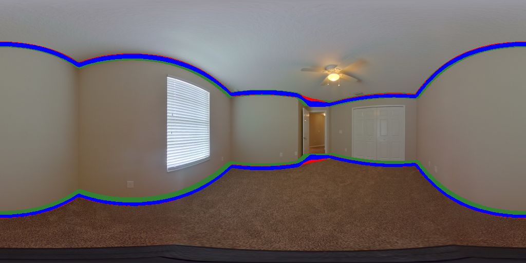
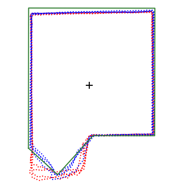
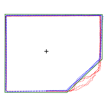
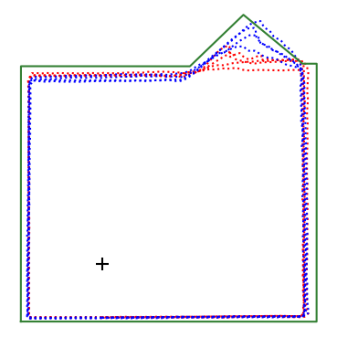
$\bullet$ Ground-truth   $\bullet$ Basic aug.   $\bullet$ With rand. perturb.
$\dagger$ The result variations are due to the four different training seeds.

Figure 6: Manhattan bias. The training set only consists of right-angled room layouts. The model, without random layout perturbation, ‘panics’ when the input is not Manhattan-aligned.

5 Conclusion and discussions

We present Seg2Reg, a novel approach to 360${}^{\circ}\,$room layout reconstruction that integrates the strengths of both segmentation and regression methods. By formulating the per-pixel 2D prediction as a floor-plan density field, we can apply our ‘flattened’ volume rendering to render layout depth regression from the density field in a differentiable and occlusion-aware manner. Furthermore, we propose a principled method for geometric data augment on 360${}^{\circ}\,$layout task. We also contribute PanoLayoutStudio, a codebase that implements several modern deep learning techniques and reproduces recent layout estimators, establishing a fair benchmark and a stronger starting point for future research. Experimental results demonstrate that our method outperforms the previous state-of-the-art.

The success of Seg2Reg highlights the potential synergy between segmentation and regression tasks in room layout estimation. However, we have not identified the reasons why the proposed method (or maybe all segmentation-based methods) seems to favor certain backbones. We hope to see more studies investigating segmentation-based layout estimators in the future. Regarding data augmentation, we instantiate two new data augmentations out of the proposed $\mathrm{LayoutWarp}$, but the potential for customization through different layout transformation functions remains largely unexplored. We encourage future extensions to a more diverse set of 360${}^{\circ}\,$layout data augmentations.

Our method introduces volume rendering into the realm of 360${}^{\circ}\,$layout estimation, paving the way for future research to leverage and adapt techniques from the NeRF [27] community. Promising avenues include exploring concepts from NeRF-based mesh reconstruction [30, 41, 46] or incorporating regularizations from few-shot NeRF [17, 29, 44].

Supplementary Material

The coordinate system used in this work is explained in detail in Sec. 6. In Sec. 7, we show the results under various setups of the baseline models reproduced by our PanoLayoutStudio. Additional technical details about layout 3D warping and Seg2Reg can be found in Sec. 8 and Sec. 9. Finally, we present an extensive qualitative comparison in Sec. 10.

6 Coordinate system

As we only consider a single image, the camera position is set as the world origin. We use a $z$-down positive world coordinate system where the positive $z$ points toward the floor.

Image to world.

Let $i,j$ be the image row and column index of a pixel. We can transform them into spherical coordinates by

$$u =\left(\frac{(j+0.5)}{W}-0.5\right)\cdot 2\pi~{},$$ (17a)

$$v =\left(\frac{(i+0.5)}{H}-0.5\right)\cdot\pi~{},$$ (17b)

where $u$ is azimuthal angle and $v$ is the angel with respect to the $xy$-plane. We can then lift the pixel to 3D by

$$x =d\cdot\cos(v)\sin(u)~{},$$ (18a)

$$y =d\cdot\cos(v)\cos(u)~{},$$ (18b)

$$z =d\cdot\sin(v)~{},$$ (18c)

where $d$ is the pixel depth.

World to image.

The inverse transformation of Eq. 18 is

$$u =\mathrm{arctan2}(x,y)~{},$$ (19a)

$$v =\mathrm{arctan2}\left(z,\sqrt{x^{2}+y^{2}}\right)~{},$$ (19b)

which is used in the operation $\mathrm{EqProj}$ (main paper Eq. (2d)) to project sampled 3D points on the floor or the ceiling planes back to the equirectangular image for density interpolation.

7 Baseline tuning

We implement HorizonNet [35], HoHoNet [36], LED2Net [39], and LGTNet [18] into our codebase—PanoLayoutStudio. In this section, we explore various setups of these reproduced baselines and evaluate on MatterportLayout [55] valid set. We use a unified training recipe for all the methods—Adam optimizer with $1\mathrm{e}{-4}$ learning rate trained for 1k epochs. We activate Stochastic Weight Averaging [16] in the last 200 epochs to stabilize training. Except stated otherwise, we use the basic setup with LGT-Net [18]—ResNet-34 as backbone; standard left-right flip, circular shifting, PanoStretch [35], and luminance jittering as data augmentation. We accumulate the results from different training seeds as box plots.

Backbones.

We show the results with different backbones, including ResNet [11] and the more advanced HRNet [40], ConvNeXt [25], and SwinTransformer [24], in Fig. 7. Overall, HRNet performs especially well in this task; ConvNeXt is slightly above ResNet; the SwinTransformer backbone seems to be unsuitable for this task. Increasing the number of backbone layers offers limited merits. The result with ResNet101 is even worse than ResNet34. Please note that all the results are trained with the same recipe. It could be possible that larger models or different network architectures need different training recipes. More future research about the different network architectures for this task would be valuable.

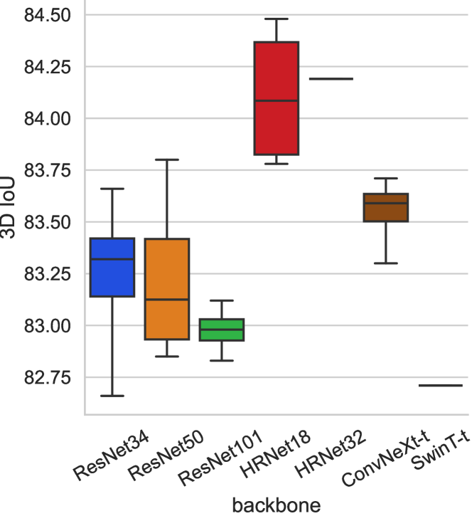
Figure 7: Results of different backbones. The results of HRNet32 and SwinT-t are obtained from only one training seed.

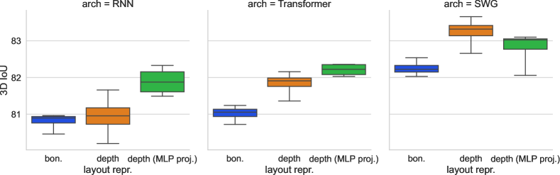
Figure 8: Results of the regression-based methods. Originally, RNN is employed by HorizonNet, Transformer is employed by HoHoNet, and SWG is proposed by LGT-Net as the 1D decoder. The layout representation ‘bon’ indicates predicting per-column layout boundary on the image space while ‘depth’ is for per-column layout depth. ‘MLP proj.‘ indicates two non-linear layers are added at the very end of the decoder before predicting the layout.

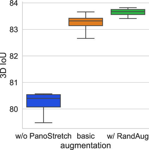
Figure 9: Results of modified basic data augmentations. PanoStretch is crucial to recent methods to achieve state-of-the-art results. Employing RandAug can further improve the result.

1D decoder and model head.

We decouple the regression-based decoder into the architecture and the layout representations. The results are presented in Fig. 8. The 1D network architecture of HorizonNet [35], HoHoNet [36], and LGTNet [18] are RNN [32], Transformer [38], and SWG (an adaptation of Swin-transformer [24]), respectively. HorizonNet proposes to predict per-column layout boundary on image space, while LGT-Net proposes to predict per-column layout depth with a layout height. For the architecture, SWG significantly outperforms Transformer and RNN. Directly predicting layout depth consistently improves the results from all architectures compared to predicting layout boundary on the image space. Originally, the features from all the architecture are just followed by a linear projection layer to predict layout. We also try to add two additional non-linear MLP layers, which improve RNN and Transformer decoder but degrade SWG results.

Interestingly, we find directly training SWG decoder to predict layout boundary fails to converge. We find it is because i) the output variance of SWG is high, and ii) the layout boundary prediction uses sigmoid to constraint the output range. The combination of these two causes the last layer to ‘die’ as predicting a large absolute value receives zero gradient from the sigmoid function. As a workaround, we multiply the output value of SWG by $0.1$ for the layout boundary prediction. The result suggests that predicting layout boundary may be more unstable compared to predicting layout depth, which may be one of the reason for the superiority of predicting layout depth.

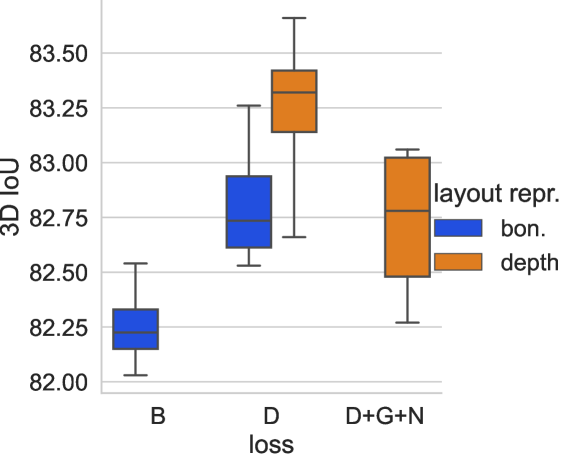
Figure 10: Results of regression training loss. Training with layout depth loss improves results even when the model predicts layout boundary on image space. Directly predicting layout depth achieves the best result. Adding gradient and normal losses to regularize layout depth does not improve.

Augmentations.

The basic augmentation consists of left-right flip, circular shifting, PanoStretch [35], and luminance jittering. In Fig. 9, we show the results of ablating PanoStretch and replacing luminance jittering with the modified modified RandAug [6]. The results show that PanoStretch is crucial to the quality, highlighting the importance of geometric-based data augmentation. Using RandAug introduces a more diverse image appearance and improves results further.

Losses.

We explore existing training losses for regression-based methods. The result is presented in Fig. 10. LED²-Net [39] proposes to render layout depth from the predicted layout boundary on the image space, which we find indeed can improve boundary prediction quality. We try the gradient and normal losses employed by LGT-Net [18] but do not observe improvement in our reproduction.

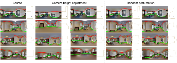
Figure 11: More visualization of the new data augmentations by $\mathrm{LayoutWarp}$

8 Layout 3D warping—more details

The proposed $\mathrm{LayoutWarp}$ (main paper Eq. (16)) enables us to produce more diverse geometrically augmented views by crafting layout polygon transformation functions $\mathrm{T}_{\mathbf{v}}$ and layout height transformation functions $\mathrm{T}_{h}$. In the following, we detail how we compute the source image coordinates from the destination image based on the given transformation so that we can apply backward warping to form the transformed image.

Source image coordinate computation.

Recap that $\mathrm{LayoutWarp}$ takes a source image $\mathcal{I}$ and it’s layout polygon $\{\mathbf{v}_{i}\}_{i=1}^{K}$, layout height $h$, and their transformation functions $\mathrm{T}_{\mathbf{v}},\mathrm{T}_{h}$ as input to form the warped image $\mathcal{I}^{\prime}$:

$$\mathcal{I}^{\prime}=\mathrm{LayoutWarp}\left(\mathcal{I},\{\mathbf{v}_{i}\}_{i=1}^{K},h,\mathrm{T}_{\mathbf{v}},\mathrm{T}_{h}\right)~{}.$$

Let

$$\{\mathbf{v}_{i}^{\prime}\}_{i=1}^{K} =\mathrm{T}_{\mathbf{v}}\left(\{\mathbf{v}_{i}\}_{i=1}^{K}\right)~{},$$ (20a)

$$h^{\prime} =\mathrm{T}_{h}\left(h\right)~{},$$ (20b)

where $\{\mathbf{v}^{\prime}\}_{i=1}^{K}$ and $h^{\prime}$ are the transformed layout polygon coordinates and layout height. To do backward warping, for each target pixel $(i^{\prime},j^{\prime})$ at the destination image, we want to compute its corresponding coordinate $(i,j)$ on the source image following the given layout transformation. We first use Eq. 17 to compute the spherical coordinate $(u^{\prime},v^{\prime})$ of the target pixel. By casting a 2D ray following the azimuthal angle $u^{\prime}$, we can find the ray-polygon intersection point $\hat{\mathbf{v}}$ on the $k$-th layout polygon edge $\overline{\mathbf{v}^{\prime}_{k}\mathbf{v}^{\prime}_{k+1}}$ (let $\mathbf{v}^{\prime}_{K+1}=\mathbf{v}^{\prime}_{1}$ as the polygon is closed). The depth term in Eq. 18 is

$$d^{\prime}=\begin{cases}z^{\mathrm{(floor)}}\cdot\csc(v^{\prime}),&\text{if}\ (i^{\prime},j^{\prime})\in\text{floor}\\ \left(z^{\mathrm{(floor)}}-h^{\prime}\right)\cdot\csc(v^{\prime}),&\text{if}\ (i^{\prime},j^{\prime})\in\text{ceiling}\\ \|\hat{\mathbf{v}}\|\cdot\sec(v^{\prime}),&\text{if}\ (i^{\prime},j^{\prime})\in\text{wall}~{},\end{cases}$$ (21)

which lifts the pixel to a 3D point $(x^{\prime},y^{\prime},z^{\prime})$. The corresponding source 3D point is

$$x =ax^{\prime}+by^{\prime}~{},$$ (22a)

$$y =cx^{\prime}+dy^{\prime}~{},$$ (22b)

$$z =z^{\mathrm{(floor)}}-\frac{h}{h^{\prime}}\cdot(z^{\mathrm{(floor)}}-z^{\prime})~{},$$ (22c)

where the backward transformation parameters $a,b,c,d$ align $\overline{\mathbf{v}^{\prime}_{k}\mathbf{v}^{\prime}_{k+1}}$ to $\overline{\mathbf{v}_{k}\mathbf{v}_{k+1}}$. Let $\mathbf{v}^{\prime}_{k}=(x^{\prime}_{k},y^{\prime}_{k})$ and $\mathbf{v}_{k}=(x_{k},y_{k})$, we solve the following linear system:

$$\begin{bmatrix}x^{\prime}_{k}&y^{\prime}_{k}&0&0\\ 0&0&x^{\prime}_{k}&y^{\prime}_{k}\\ x^{\prime}_{k+1}&y^{\prime}_{k+1}&0&0\\ 0&0&x^{\prime}_{k+1}&y^{\prime}_{k+1}\\ \end{bmatrix}\begin{bmatrix}a\\ b\\ c\\ d\end{bmatrix}=\begin{bmatrix}x_{k}\\ y_{k}\\ x_{k+1}\\ y_{k+1}\end{bmatrix}~{},$$ (23)

where the solution is

$$a =\frac{y^{\prime}_{k+1}\cdot x_{k}-y^{\prime}_{k}\cdot x_{k+1}}{y^{\prime}_{k+1}\cdot x^{\prime}_{k}-y^{\prime}_{k}\cdot x^{\prime}_{k+1}}~{},$$ (24a)

$$b =\frac{x^{\prime}_{k+1}\cdot x_{k}-x^{\prime}_{k}\cdot x_{k+1}}{x^{\prime}_{k+1}\cdot y^{\prime}_{k}-x^{\prime}_{k}\cdot y^{\prime}_{k+1}}~{},$$ (24b)

$$c =\frac{y^{\prime}_{k+1}\cdot y_{k}-y^{\prime}_{k}\cdot y_{k+1}}{y^{\prime}_{k+1}\cdot x^{\prime}_{k}-y^{\prime}_{k}\cdot x^{\prime}_{k+1}}~{},$$ (24c)

$$d =\frac{x^{\prime}_{k+1}\cdot y_{k}-x^{\prime}_{k}\cdot y_{k+1}}{x^{\prime}_{k+1}\cdot y^{\prime}_{k}-x^{\prime}_{k}\cdot y^{\prime}_{k+1}}~{}.$$ (24d)

Note that we assume $\mathbf{v}_{k}\neq\mathbf{v}_{k+1}$ and $\mathbf{v}^{\prime}_{k}\neq\mathbf{v}^{\prime}_{k+1}$ for all layout polygon edges. Finally, the corresponding source 3D point $(x,y,z)$ from Eq. 22 is projected to the source image using Eq. 19 to interpolate the color.

Effect	$\mathrm{T}_{\mathbf{v}}$	$\mathrm{T}_{h}$
Left-right circular shifting	$\mathbf{v}^{\prime}_{k}=\begin{bmatrix}\cos(\theta)&-\sin(\theta)\\ \sin(\theta)&\cos(\theta)\end{bmatrix}\mathbf{v}_{k}$	$h^{\prime}=h$
† The rotation $\theta$ is shared by all the $K$ vertices.
Left-right flip	$\mathbf{v}^{\prime}_{k}=\begin{bmatrix}-1&0\\ 0&1\end{bmatrix}\mathbf{v}_{k}$	$h^{\prime}=h$
PanoStretch [35]	$\mathbf{v}^{\prime}_{k}=\begin{bmatrix}s_{x}&0\\ 0&s_{y}\end{bmatrix}\mathbf{v}_{k}$	$h^{\prime}=h$
† The scaling factors $s_{x},s_{y}$ are shared by all the $K$ vertices.
Camera height adjustment	$\mathbf{v}^{\prime}_{k}=s\mathbf{v}_{k}$	$h^{\prime}=sh$
† The $s$ scales camera height by $\frac{1}{s}$ and is shared by all vertices and height.
Random perturbation	$\mathbf{v}^{\prime}_{k}=s_{k}\mathbf{v}_{k}$	$h^{\prime}=h$
† Each of the $K$ vertex has it’s own scaling factor.

Table 5: Geometric-based data augmentation by $\mathrm{LayoutWarp}$.

$\bullet$ Ground-truth   $\bullet$ Basic aug.   $\bullet$ With rand. perturb.

$\dagger$ The result variations are due to the four different training seeds.

Figure 12: Training with random perturbation generalizes better from Manhattan to general layout. We can observe that the models trained with random perturbation are less ‘panics’ when the input is not Manhattan-aligned.

Crafting the transformation functions.

We can craft $\mathrm{T}_{\mathbf{v}},\mathrm{T}_{h}$ to produce various geometric augmentations. We summarize the realization of the commonly-used left-right circular shifting, left-right flip, PanoStretch [35], and the new camera height adjustment and random layout polygon perturbation in Tab. 5. We visualize more augmented views in Fig. 11.

More qualitative comparison of random perturbation.

In the main paper, we show random perturbation can improve the results when generalizing from a Manhattan-aligned dataset to a general layout dataset. We show more visual comparison in Fig. 12.

9 Seg2Reg—more details

We provide more technical details and analyses of the proposed Seg2Reg in this section.

Training details.

Our Seg2Reg enables differentiable layout depth (i.e., distance to layout wall on the floor plan) rendering from the 2D density map prediction. The ‘flattened’ volume rendering is detailed in the main paper Sec. 3.1. Directly supervising the rendering by ground-truth layout depth leads to ambiguity. Recap that the depth rendering equation of a ray is (main paper Eq.(3)):

$$d=\sum\nolimits_{i=1}^{K}T_{i}\alpha_{i}t_{i}~{},\text{where}~{}T_{i}=\prod\nolimits_{j=1}^{i-1}\left(1-\alpha_{j}\right)~{},$$

where $K$ is the number of sampled points on the ray. We can see that there are an infinite number of weight distributions on the ray that can render to a specific ground-truth depth $d^{*}$. To resolve ambiguity, we directly derive a compact weight distribution $w^{*}$ for the ground-truth depth $d^{*}$. Let $t_{k},t_{k+1}$ be the two depth values nearest to $d^{*}$ on the ray. Our ground truth weight distribution is:

$$w_{k} =\frac{t_{k+1}-d^{*}}{t_{k+1}-t_{k}}~{},$$ (25a)

$$w_{k+1} =1-w_{k}~{},$$ (25b)

$$w_{i} =0~{},\text{where}~{}i=1,\cdots,k{-}1,k{+}2,\cdots,K+1~{}.$$ (25c)

There is a special case when the far clipping distance of the ray does not reach the layout $t_{K}<d^{*}$. In this special case, the weights are all zero except $W_{K+1}=1$.

To render the primary layout, we directly use the $\frac{H}{2}$ points in the image column as the sampled points. For the secondary layouts, we sample $N^{\mathrm{(secondary)}}=32$ secondary camera centers. To render layout depth for the secondary cameras, we uniformly sampled $1{,}024$ points on a ray with the farthest distance $t_{K}=16$ (the camera-to-floor distance is $z^{\mathrm{(floor)}}=1.6$). The loss weights for $\mathcal{L}^{\mathrm{(pri.)}}$, $\mathcal{L}^{\mathrm{(2nd)}}$, and $\mathcal{L}^{\mathrm{(seg.)}}$ are $w_{1}=1.0,w_{2}=0.1,w_{3}=1.0$, respectively.

Robust polygons merging algorithm.

To merge the primary layout polygon and secondary layout polygons, the simplest way is to directly take the polygon union. Such a naive strategy may have polygon edges crossing the region outside the layout where the model actually predicts high floor plan density (the red polygon in the figure), especially when the rendered secondary polygons are in lower resolution (fewer number of vertices). This prompts us to design a more robust algorithm. Our idea is to connect all the rendered vertices with the minimum perimeter. We first compute the pair-wise distance matrix of all the rendered vertices from primary and secondary views. The pair-wise distance matrix represents a complete graph. We then construct a minimum spanning tree from the complete graph via the Kruskal algorithm. The final merged polygon (the green polygon in the figure) is determined by the trajectory connecting the farthest two points on the tree, which can be realized by running the depth-first tree search two times.

We show the results of the two polygon merging methods and the result after polygon simplification in Tab. 6.

Union	MST	MST + simplification
87.22%	87.33%	87.13%

Table 6: Results of different polygon merging algorithms. We report the 2DIoU$\uparrow$ comparison on MatterportLayout valid set. Polygon merging via minimum spanning tree (MST) achieves slightly better results. Applying polygon simplification causes the number result to drop slightly.

Raw prediction visualizations.

In the main paper’s Table.3, we show that our Seg2Reg achieves better quantitative results than a purely segmentation-based method. In Fig. 13, we visualize the raw predictions activated by $\mathrm{Sigmoid}$. Segmentation-based method only supervises per-pixel classification. The proposed Seg2Reg introduces rendering loss, which emphasizes the rendered polygon position, while the density far outside the layout polygon is less important as they do not affect the rendering results.

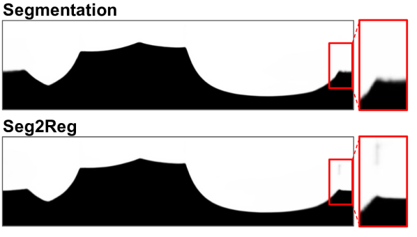
Figure 13: Visualization of the raw predictions. Segmentation-only method and our Seg2Reg converge to different results.

10 Qualitative comparison

We provide an extensive qualitative comparison in Fig. 14. We run LGT-Net’s official repo to show the performance of the existing state-of-the-art.

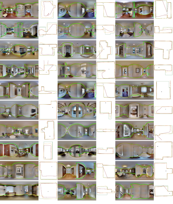
$\bullet$ Ground-truth   $\bullet$ Seg2Reg   $\bullet$ LGT-Net

Figure 14: Qualitative comparisons on the unseen data from MatterportLayout. We compare it with the state-of-the-art model from LGT-Net’s official repo. The test set 2DIoU is $83.52$% for the official LGT-Net and $85.14$% for our model.

References

- Armeni et al. [2017] Iro Armeni, Sasha Sax, Amir R. Zamir, and Silvio Savarese. Joint 2d-3d-semantic data for indoor scene understanding. CoRR, abs/1702.01105, 2017.
- Chang et al. [2017] Angel X. Chang, Angela Dai, Thomas A. Funkhouser, Maciej Halber, Matthias Nießner, Manolis Savva, Shuran Song, Andy Zeng, and Yinda Zhang. Matterport3d: Learning from RGB-D data in indoor environments. In 2017 International Conference on 3D Vision, 3DV 2017, Qingdao, China, October 10-12, 2017, pages 667–676. IEEE Computer Society, 2017.
- Chen et al. [2022] Anpei Chen, Zexiang Xu, Andreas Geiger, Jingyi Yu, and Hao Su. Tensorf: Tensorial radiance fields. In Computer Vision - ECCV 2022 - 17th European Conference, Tel Aviv, Israel, October 23-27, 2022, Proceedings, Part XXXII, pages 333–350. Springer, 2022.
- Cruz et al. [2021] Steve Cruz, Will Hutchcroft, Yuguang Li, Naji Khosravan, Ivaylo Boyadzhiev, and Sing Bing Kang. Zillow indoor dataset: Annotated floor plans with 360deg panoramas and 3d room layouts. In IEEE Conference on Computer Vision and Pattern Recognition, CVPR 2021, virtual, June 19-25, 2021, pages 2133–2143. Computer Vision Foundation / IEEE, 2021.
- Cubuk et al. [2019] Ekin D. Cubuk, Barret Zoph, Dandelion Mané, Vijay Vasudevan, and Quoc V. Le. Autoaugment: Learning augmentation strategies from data. In IEEE Conference on Computer Vision and Pattern Recognition, CVPR 2019, Long Beach, CA, USA, June 16-20, 2019, pages 113–123. Computer Vision Foundation / IEEE, 2019.
- Cubuk et al. [2020] Ekin D. Cubuk, Barret Zoph, Jonathon Shlens, and Quoc V. Le. Randaugment: Practical automated data augmentation with a reduced search space. In 2020 IEEE/CVF Conference on Computer Vision and Pattern Recognition, CVPR Workshops 2020, Seattle, WA, USA, June 14-19, 2020, pages 3008–3017. Computer Vision Foundation / IEEE, 2020.
- Dabouei et al. [2021] Ali Dabouei, Sobhan Soleymani, Fariborz Taherkhani, and Nasser M. Nasrabadi. Supermix: Supervising the mixing data augmentation. In IEEE Conference on Computer Vision and Pattern Recognition, CVPR 2021, virtual, June 19-25, 2021, pages 13794–13803. Computer Vision Foundation / IEEE, 2021.
- Fernandez-Labrador et al. [2020] Clara Fernandez-Labrador, José M. Fácil, Alejandro Pérez-Yus, Cédric Demonceaux, Javier Civera, and José Jesús Guerrero. Corners for layout: End-to-end layout recovery from 360 images. IEEE Robotics Autom. Lett., 5(2):1255–1262, 2020.
- Fridovich-Keil et al. [2022] Sara Fridovich-Keil, Alex Yu, Matthew Tancik, Qinhong Chen, Benjamin Recht, and Angjoo Kanazawa. Plenoxels: Radiance fields without neural networks. In IEEE/CVF Conference on Computer Vision and Pattern Recognition, CVPR 2022, New Orleans, LA, USA, June 18-24, 2022, pages 5491–5500. IEEE, 2022.
- Gao et al. [2022] Chao-Chen Gao, Cheng-Hsiu Chen, Jheng-Wei Su, and Hung-Kuo Chu. Layout-guided indoor panorama inpainting with plane-aware normalization. In Computer Vision - ACCV 2022 - 16th Asian Conference on Computer Vision, Macao, China, December 4-8, 2022, Proceedings, Part VI, pages 425–441. Springer, 2022.
- He et al. [2016] Kaiming He, Xiangyu Zhang, Shaoqing Ren, and Jian Sun. Deep residual learning for image recognition. In 2016 IEEE Conference on Computer Vision and Pattern Recognition, CVPR 2016, Las Vegas, NV, USA, June 27-30, 2016, pages 770–778. IEEE Computer Society, 2016.
- Hoffer et al. [2020] Elad Hoffer, Tal Ben-Nun, Itay Hubara, Niv Giladi, Torsten Hoefler, and Daniel Soudry. Augment your batch: Improving generalization through instance repetition. In 2020 IEEE/CVF Conference on Computer Vision and Pattern Recognition, CVPR 2020, Seattle, WA, USA, June 13-19, 2020, pages 8126–8135. Computer Vision Foundation / IEEE, 2020.
- Hsieh et al. [2023] Yu-Cheng Hsieh, Cheng Sun, Suraj Dengale, and Min Sun. Panomixswap panorama mixing via structural swapping for indoor scene understanding. CoRR, abs/2309.09514, 2023.
- Hutchcroft et al. [2022] Will Hutchcroft, Yuguang Li, Ivaylo Boyadzhiev, Zhiqiang Wan, Haiyan Wang, and Sing Bing Kang. Covispose: Co-visibility pose transformer for wide-baseline relative pose estimation in 360$^\circ $ indoor panoramas. In Computer Vision - ECCV 2022 - 17th European Conference, Tel Aviv, Israel, October 23-27, 2022, Proceedings, Part XXXII, pages 615–633. Springer, 2022.
- Izadinia et al. [2017] Hamid Izadinia, Qi Shan, and Steven M. Seitz. IM2CAD. In 2017 IEEE Conference on Computer Vision and Pattern Recognition, CVPR 2017, Honolulu, HI, USA, July 21-26, 2017, pages 2422–2431. IEEE Computer Society, 2017.
- Izmailov et al. [2018] Pavel Izmailov, Dmitrii Podoprikhin, Timur Garipov, Dmitry P. Vetrov, and Andrew Gordon Wilson. Averaging weights leads to wider optima and better generalization. In Proceedings of the Thirty-Fourth Conference on Uncertainty in Artificial Intelligence, UAI 2018, Monterey, California, USA, August 6-10, 2018, pages 876–885. AUAI Press, 2018.
- Jain et al. [2021] Ajay Jain, Matthew Tancik, and Pieter Abbeel. Putting nerf on a diet: Semantically consistent few-shot view synthesis. In 2021 IEEE/CVF International Conference on Computer Vision, ICCV 2021, Montreal, QC, Canada, October 10-17, 2021, pages 5865–5874. IEEE, 2021.
- Jiang et al. [2022] Zhigang Jiang, Zhongzheng Xiang, Jinhua Xu, and Ming Zhao. Lgt-net: Indoor panoramic room layout estimation with geometry-aware transformer network. In IEEE/CVF Conference on Computer Vision and Pattern Recognition, CVPR 2022, New Orleans, LA, USA, June 18-24, 2022, pages 1644–1653. IEEE, 2022.
- Kajiya and Herzen [1984] James T. Kajiya and Brian Von Herzen. Ray tracing volume densities. In Proceedings of the 11th Annual Conference on Computer Graphics and Interactive Techniques, SIGGRAPH 1984, Minneapolis, Minnesota, USA, July 23-27, 1984, pages 165–174. ACM, 1984.
- Kingma and Ba [2015] Diederik P. Kingma and Jimmy Ba. Adam: A method for stochastic optimization. In 3rd International Conference on Learning Representations, ICLR 2015, San Diego, CA, USA, May 7-9, 2015, Conference Track Proceedings, 2015.
- Lee et al. [2017] Chen-Yu Lee, Vijay Badrinarayanan, Tomasz Malisiewicz, and Andrew Rabinovich. Roomnet: End-to-end room layout estimation. In IEEE International Conference on Computer Vision, ICCV 2017, Venice, Italy, October 22-29, 2017, pages 4875–4884. IEEE Computer Society, 2017.
- Li et al. [2021] Zhengqin Li, Ting-Wei Yu, Shen Sang, Sarah Wang, Meng Song, Yuhan Liu, Yu-Ying Yeh, Rui Zhu, Nitesh B. Gundavarapu, Jia Shi, Sai Bi, Hong-Xing Yu, Zexiang Xu, Kalyan Sunkavalli, Milos Hasan, Ravi Ramamoorthi, and Manmohan Chandraker. Openrooms: An open framework for photorealistic indoor scene datasets. In IEEE Conference on Computer Vision and Pattern Recognition, CVPR 2021, virtual, June 19-25, 2021, pages 7190–7199. Computer Vision Foundation / IEEE, 2021.
- Lim et al. [2019] Sungbin Lim, Ildoo Kim, Taesup Kim, Chiheon Kim, and Sungwoong Kim. Fast autoaugment. In Advances in Neural Information Processing Systems 32: Annual Conference on Neural Information Processing Systems 2019, NeurIPS 2019, December 8-14, 2019, Vancouver, BC, Canada, pages 6662–6672, 2019.
- Liu et al. [2021] Ze Liu, Yutong Lin, Yue Cao, Han Hu, Yixuan Wei, Zheng Zhang, Stephen Lin, and Baining Guo. Swin transformer: Hierarchical vision transformer using shifted windows. In 2021 IEEE/CVF International Conference on Computer Vision, ICCV 2021, Montreal, QC, Canada, October 10-17, 2021, pages 9992–10002. IEEE, 2021.
- Liu et al. [2022] Zhuang Liu, Hanzi Mao, Chao-Yuan Wu, Christoph Feichtenhofer, Trevor Darrell, and Saining Xie. A convnet for the 2020s. In IEEE/CVF Conference on Computer Vision and Pattern Recognition, CVPR 2022, New Orleans, LA, USA, June 18-24, 2022, pages 11966–11976. IEEE, 2022.
- Max [1995] Nelson L. Max. Optical models for direct volume rendering. IEEE Trans. Vis. Comput. Graph., 1(2):99–108, 1995.
- Mildenhall et al. [2020] Ben Mildenhall, Pratul P. Srinivasan, Matthew Tancik, Jonathan T. Barron, Ravi Ramamoorthi, and Ren Ng. Nerf: Representing scenes as neural radiance fields for view synthesis. In Computer Vision - ECCV 2020 - 16th European Conference, Glasgow, UK, August 23-28, 2020, Proceedings, Part I, pages 405–421. Springer, 2020.
- Müller et al. [2022] Thomas Müller, Alex Evans, Christoph Schied, and Alexander Keller. Instant neural graphics primitives with a multiresolution hash encoding. ACM Trans. Graph., 41(4):102:1–102:15, 2022.
- Niemeyer et al. [2022] Michael Niemeyer, Jonathan T. Barron, Ben Mildenhall, Mehdi S. M. Sajjadi, Andreas Geiger, and Noha Radwan. Regnerf: Regularizing neural radiance fields for view synthesis from sparse inputs. In IEEE/CVF Conference on Computer Vision and Pattern Recognition, CVPR 2022, New Orleans, LA, USA, June 18-24, 2022, pages 5470–5480. IEEE, 2022.
- Oechsle et al. [2021] Michael Oechsle, Songyou Peng, and Andreas Geiger. UNISURF: unifying neural implicit surfaces and radiance fields for multi-view reconstruction. In 2021 IEEE/CVF International Conference on Computer Vision, ICCV 2021, Montreal, QC, Canada, October 10-17, 2021, pages 5569–5579. IEEE, 2021.
- Pintore et al. [2020] Giovanni Pintore, Marco Agus, and Enrico Gobbetti. Atlantanet: Inferring the 3d indoor layout from a single $360^\circ $ image beyond the manhattan world assumption. In Computer Vision - ECCV 2020 - 16th European Conference, Glasgow, UK, August 23-28, 2020, Proceedings, Part VIII, pages 432–448. Springer, 2020.
- Schuster and Paliwal [1997] Mike Schuster and Kuldip K Paliwal. Bidirectional recurrent neural networks. In IEEE Transactions on Signal Processing, 1997.
- Shabani et al. [2021] Mohammad Amin Shabani, Weilian Song, Makoto Odamaki, Hirochika Fujiki, and Yasutaka Furukawa. Extreme structure from motion for indoor panoramas without visual overlaps. In 2021 IEEE/CVF International Conference on Computer Vision, ICCV 2021, Montreal, QC, Canada, October 10-17, 2021, pages 5683–5691. IEEE, 2021.
- Solarte et al. [2022] Bolivar Solarte, Yueh-Cheng Liu, Chin-Hsuan Wu, Yi-Hsuan Tsai, and Min Sun. 360-dfpe: Leveraging monocular 360-layouts for direct floor plan estimation. IEEE Robotics Autom. Lett., 7(3):6503–6510, 2022.
- Sun et al. [2019] Cheng Sun, Chi-Wei Hsiao, Min Sun, and Hwann-Tzong Chen. Horizonnet: Learning room layout with 1d representation and pano stretch data augmentation. In IEEE Conference on Computer Vision and Pattern Recognition, CVPR 2019, Long Beach, CA, USA, June 16-20, 2019, pages 1047–1056. Computer Vision Foundation / IEEE, 2019.
- Sun et al. [2021] Cheng Sun, Min Sun, and Hwann-Tzong Chen. Hohonet: 360 indoor holistic understanding with latent horizontal features. In IEEE Conference on Computer Vision and Pattern Recognition, CVPR 2021, virtual, June 19-25, 2021, pages 2573–2582. Computer Vision Foundation / IEEE, 2021.
- Sun et al. [2022] Cheng Sun, Min Sun, and Hwann-Tzong Chen. Direct voxel grid optimization: Super-fast convergence for radiance fields reconstruction. In IEEE/CVF Conference on Computer Vision and Pattern Recognition, CVPR 2022, New Orleans, LA, USA, June 18-24, 2022, pages 5449–5459. IEEE, 2022.
- Vaswani et al. [2017] Ashish Vaswani, Noam Shazeer, Niki Parmar, Jakob Uszkoreit, Llion Jones, Aidan N. Gomez, Lukasz Kaiser, and Illia Polosukhin. Attention is all you need. In Advances in Neural Information Processing Systems 30: Annual Conference on Neural Information Processing Systems 2017, 4-9 December 2017, Long Beach, CA, USA, pages 5998–6008, 2017.
- Wang et al. [2021a] Fu-En Wang, Yu-Hsuan Yeh, Min Sun, Wei-Chen Chiu, and Yi-Hsuan Tsai. Led2-net: Monocular 360deg layout estimation via differentiable depth rendering. In IEEE Conference on Computer Vision and Pattern Recognition, CVPR 2021, virtual, June 19-25, 2021, pages 12956–12965. Computer Vision Foundation / IEEE, 2021a.
- Wang et al. [2021b] Jingdong Wang, Ke Sun, Tianheng Cheng, Borui Jiang, Chaorui Deng, Yang Zhao, Dong Liu, Yadong Mu, Mingkui Tan, Xinggang Wang, Wenyu Liu, and Bin Xiao. Deep high-resolution representation learning for visual recognition. IEEE Trans. Pattern Anal. Mach. Intell., 43(10):3349–3364, 2021b.
- Wang et al. [2021c] Peng Wang, Lingjie Liu, Yuan Liu, Christian Theobalt, Taku Komura, and Wenping Wang. Neus: Learning neural implicit surfaces by volume rendering for multi-view reconstruction. In Advances in Neural Information Processing Systems 34: Annual Conference on Neural Information Processing Systems 2021, NeurIPS 2021, December 6-14, 2021, virtual, pages 27171–27183, 2021c.
- Xie et al. [2021] Enze Xie, Wenhai Wang, Zhiding Yu, Anima Anandkumar, José M. Álvarez, and Ping Luo. Segformer: Simple and efficient design for semantic segmentation with transformers. In Advances in Neural Information Processing Systems 34: Annual Conference on Neural Information Processing Systems 2021, NeurIPS 2021, December 6-14, 2021, virtual, pages 12077–12090, 2021.
- Xu et al. [2021] Jiale Xu, Jia Zheng, Yanyu Xu, Rui Tang, and Shenghua Gao. Layout-guided novel view synthesis from a single indoor panorama. In IEEE Conference on Computer Vision and Pattern Recognition, CVPR 2021, virtual, June 19-25, 2021, pages 16438–16447. Computer Vision Foundation / IEEE, 2021.
- Yang et al. [2023] Jiawei Yang, Marco Pavone, and Yue Wang. Freenerf: Improving few-shot neural rendering with free frequency regularization. In IEEE/CVF Conference on Computer Vision and Pattern Recognition, CVPR 2023, Vancouver, BC, Canada, June 17-24, 2023, pages 8254–8263. IEEE, 2023.
- Yang et al. [2019] Shang-Ta Yang, Fu-En Wang, Chi-Han Peng, Peter Wonka, Min Sun, and Hung-Kuo Chu. Dula-net: A dual-projection network for estimating room layouts from a single RGB panorama. In IEEE Conference on Computer Vision and Pattern Recognition, CVPR 2019, Long Beach, CA, USA, June 16-20, 2019, pages 3363–3372. Computer Vision Foundation / IEEE, 2019.
- Yariv et al. [2021] Lior Yariv, Jiatao Gu, Yoni Kasten, and Yaron Lipman. Volume rendering of neural implicit surfaces. In Advances in Neural Information Processing Systems 34: Annual Conference on Neural Information Processing Systems 2021, NeurIPS 2021, December 6-14, 2021, virtual, pages 4805–4815, 2021.
- Yeh et al. [2022] Yu-Ying Yeh, Zhengqin Li, Yannick Hold-Geoffroy, Rui Zhu, Zexiang Xu, Milos Hasan, Kalyan Sunkavalli, and Manmohan Chandraker. Photoscene: Photorealistic material and lighting transfer for indoor scenes. In IEEE/CVF Conference on Computer Vision and Pattern Recognition, CVPR 2022, New Orleans, LA, USA, June 18-24, 2022, pages 18541–18550. IEEE, 2022.
- Yun et al. [2019] Sangdoo Yun, Dongyoon Han, Sanghyuk Chun, Seong Joon Oh, Youngjoon Yoo, and Junsuk Choe. Cutmix: Regularization strategy to train strong classifiers with localizable features. In 2019 IEEE/CVF International Conference on Computer Vision, ICCV 2019, Seoul, Korea (South), October 27 - November 2, 2019, pages 6022–6031. IEEE, 2019.
- Zhang et al. [2021] Cheng Zhang, Zhaopeng Cui, Cai Chen, Shuaicheng Liu, Bing Zeng, Hujun Bao, and Yinda Zhang. Deeppanocontext: Panoramic 3d scene understanding with holistic scene context graph and relation-based optimization. In 2021 IEEE/CVF International Conference on Computer Vision, ICCV 2021, Montreal, QC, Canada, October 10-17, 2021, pages 12612–12621. IEEE, 2021.
- Zhang et al. [2018] Hongyi Zhang, Moustapha Cissé, Yann N. Dauphin, and David Lopez-Paz. mixup: Beyond empirical risk minimization. In 6th International Conference on Learning Representations, ICLR 2018, Vancouver, BC, Canada, April 30 - May 3, 2018, Conference Track Proceedings. OpenReview.net, 2018.
- Zhang et al. [2014] Yinda Zhang, Shuran Song, Ping Tan, and Jianxiong Xiao. Panocontext: A whole-room 3d context model for panoramic scene understanding. In Computer Vision - ECCV 2014 - 13th European Conference, Zurich, Switzerland, September 6-12, 2014, Proceedings, Part VI, pages 668–686. Springer, 2014.
- Zhao et al. [2017] Hao Zhao, Ming Lu, Anbang Yao, Yiwen Guo, Yurong Chen, and Li Zhang. Physics inspired optimization on semantic transfer features: An alternative method for room layout estimation. In 2017 IEEE Conference on Computer Vision and Pattern Recognition, CVPR 2017, Honolulu, HI, USA, July 21-26, 2017, pages 870–878. IEEE Computer Society, 2017.
- Zhong et al. [2020] Zhun Zhong, Liang Zheng, Guoliang Kang, Shaozi Li, and Yi Yang. Random erasing data augmentation. In The Thirty-Fourth AAAI Conference on Artificial Intelligence, AAAI 2020, The Thirty-Second Innovative Applications of Artificial Intelligence Conference, IAAI 2020, The Tenth AAAI Symposium on Educational Advances in Artificial Intelligence, EAAI 2020, New York, NY, USA, February 7-12, 2020, pages 13001–13008. AAAI Press, 2020.
- Zou et al. [2018] Chuhang Zou, Alex Colburn, Qi Shan, and Derek Hoiem. Layoutnet: Reconstructing the 3d room layout from a single RGB image. In 2018 IEEE Conference on Computer Vision and Pattern Recognition, CVPR 2018, Salt Lake City, UT, USA, June 18-22, 2018, pages 2051–2059. Computer Vision Foundation / IEEE Computer Society, 2018.
- Zou et al. [2021] Chuhang Zou, Jheng-Wei Su, Chi-Han Peng, Alex Colburn, Qi Shan, Peter Wonka, Hung-Kuo Chu, and Derek Hoiem. Manhattan room layout reconstruction from a single $360^{\circ }$ image: A comparative study of state-of-the-art methods. Int. J. Comput. Vis., 129(5):1410–1431, 2021.