[a,b]Pietro Butti
Testing (asymptotic) scaling in Yang-Mills theories in the large- limit
Abstract
TEK reduction is a well-established technique that allows single-site simulations of Yang-Mills theory in the large- limit by exploiting volume reduction induced by twisted boundary conditions. We performed simulations for for several gauge couplings and applied standard Wilson flow techniques combined with a tree-level improvement methodology to set the lattice scale. The wide range of gauge couplings covered by our simulations allows us to explore a region in the coupling space where our data exhibits asymptotic scaling and perturbation theory could be used to analyze the behaviour of the -function. In this talk, I will review the methodology used and go through the main results we obtained, including a determination of the -parameter of Yang-Mills theory at large- in -scheme.
IFT-UAM/CSIC-23-58
1 Introduction
In a generic bare-coupling definition scheme labelled by , the Renormalization Group (RG) equation for the bare ’t Hooft coupling dependence on the cutoff scale reads
| (1) |
It is well-known that the -function has the following perturbative expansion around
| (2) |
where and are known to be universal (scheme independent) and in a pure Yang-Mills theory they amount to and , while higher-order coefficients are known to be dependent on the scheme chosen. Using a fully perturbative -function truncated at , upon integration, Eq. (1) gives
| (3) |
where the coefficient of the linear term is given by , and is scheme-dependent, as well as the -parameter itself. On the lattice, it is natural to use the coupling parameter in the lattice action as a natural coupling scheme. For Wilson action we label it as . This scheme is known to have large higher-order perturbative corrections, since the ratio between the Wilson and scales is large [1, 2] . This induces large violations of the scale dependence of the coupling with respect to the truncated perturbative prediction, which we refer to as asymptotic scaling. This showed up from the earliest studies, and several authors proposed adopting a different definition of the coupling which is better behaved. These are called improved couplings. The goal of this work is to test how well the asymptotic predictions hold for the case of Yang-Mills theory in the large- limit. Our results are based upon an extensive analysis. Here we present some preliminary results. The full analysis will follow in a future publication [3].
Our strategy is to make use of the volume reduction property at large which allows to obtain results about standard gauge theory by simulations on a single site lattice with twisted boundary conditions [4, 5]. After a change of variables, the resulting Wilson action of the reduced model (TEK model) becomes
| (4) |
where are matrices, is the inverse of ’t Hooft coupling , while is a complex phase encoding the twist and given by for ( is an integer coprime with ). This particular choice of the twist factor is called symmetric twist.
The vacuum configurations for the TEK action (4) are called twist-eaters and they are given by which are the solutions of the twist equation:
| (5) |
The equivalence of the TEK model and the infinite volume large gauge theory has been proven both perturbatively and non-perturbatively. Furthermore, the proof shows that finite corrections take the form of finite volume corrections in a lattice whose effective size is [4, 5]. Thus our choice of implies a lattice of size allowing us to study the approach to the continuum limit and matching the expected behaviour of the infinite volume large gauge theory.
2 The Wilson flow scale(s)
To set the scale we use an observable which allows a simple determination with great precision. This is the gradient flow scale [6]. This is based upon evolving the gauge field with the equation , being the flow time. As observable we take the flowed energy density . On the single-site twisted lattice the evolution takes place with respect to the dimensionless lattice flow time , with the corresponding observable being
| (6) |
in terms of which we define the dimensionless observable normalized to the number of colours in order to have a finite large limit.
This observable allows to define a scale as follows
| (7) |
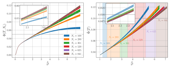
The choice of is taken as a compromise that minimizes finite volume effects (finite ) while still being very slightly affected by lattice artefacts. To exemplify this, we display in the left side of Fig. 1 the flow curves for several values of for pure Yang-Mills reduced model () at , where the two reference scales and are depicted with corresponding horizontal grey lines. As it is visible from the plot, although the scale is less affected by the -dependence of the flow, the systematic error induced is still sizeable for the smaller values of . The situation can be strongly ameliorated by the method employed in Ref. [7] to be briefly explained below.
Our approach is to consider a new lattice observable to replace , which nonetheless coincides with its infinite and vanishing lattice spacing limit. It is clear that this quantity is as good an observable as the previous one, but is expected to have smaller finite and lattice corrections. This is given by
| (8) |
where the prefactor is a function of such that . It is determined in such a way as to eliminate the dependence at the lowest order of perturbation theory. This was analytically calculated in Ref. [8]. We refer to our modified method as norm correction and we expect it to simultaneously reduce finite- and lattice artefacts in an effective window in . The lower limit is set to eliminate any interference from lattice artefacts, while the upper limit is determined by ensuring that the smearing radius remains reasonably smaller than a fraction of the overall size of the effective lattice, where residual finite-volume effects are negligible. We typically refer to this range in as the scaling window, which can be expressed as
| (9) |
After the application of the norm correction, we define in the same way but in terms of , and we extract the scale by interpolation. The right-hand side of Fig. 1 shows the effect. We observe that, apart from the case of , all the scales , interpolated from , coincide within errors, signalling that the norm-correction can effectively correct the finite-/finite-size effects. The norm-correction method was used in Ref. [7] to determine the scale from data of and . In our case, since is much larger we can safely claim that the corresponding scales amount to the corresponding one at infinite . A detailed discussion about the norm correction and its applications to the case of this and other theories can be found also in[9].
We have measured the scale for a large number of values of for the TEK model. The obtained values of are listed in the second column of Tab. 1.
We can confront the extracted scales with a previous, less precise, determination in units of the string tension given in Ref. [10]. The numbers are reported in the third column of Tab. 1. In Fig. 2, we depict each value of the dimensionless ratio as a function of .
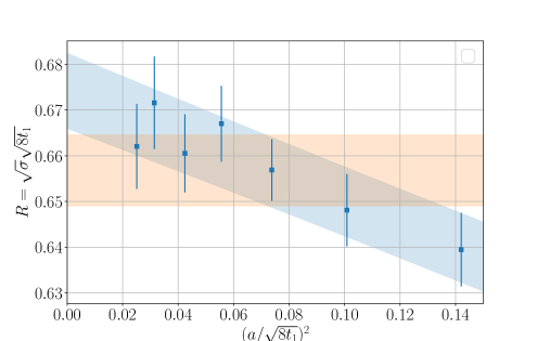
Exact scaling would imply the ratio to be constant. Such a fit has a , mainly spoiled by the value at the 2 coarsest point. Nevertheless, we notice that a linear fit in gives an and might suggest slight scaling violations. As a final value, we will consider where the systematic error is the dispersion between the two previously obtained values. This comparison with the string tension is a remarkable confirmation of the validity of scaling for a wide range of ’t Hooft couplings with only small violations in the case of the coarsest ensembles.
3 Asymptotic scaling and
In this section, we will analyze if the scales we determined follow the asymptotic predictions reviewed in the introduction. For the large theory a similar analysis was performed earlier [11, 10]. We employ three different improved couplings: (from [11]), (from [12, 13]) and , defined in Tab. 2.
| symbol | definition | ||
|---|---|---|---|
Having at our disposal such a large range of values for the ’t Hooft couplings and given the small errors of our scale determination we are certainly making stringent tests to our data. A global analysis can be done by fitting Eq. (3) to our data for the case of the scheme only leaving free the value of . The result is displayed in Fig. 3 where the data points and the continuous best-fit curve are shown. The overall impression is very good since the curve follows quite nicely the evolution of the data. However, given the small errors, the of the fit is not good. Indeed, for the range of scales covered, certain non-perturbative scaling violations are to be expected.
We aim at a determination of the parameters which are consistent with the predictions of perturbation theory. It is customary to choose as preferred scale the one coming from the scheme in the continuum: . The ratio of the -parameters in any scale to can be determined by passing through the Wilson scheme as follows:
| (10) |
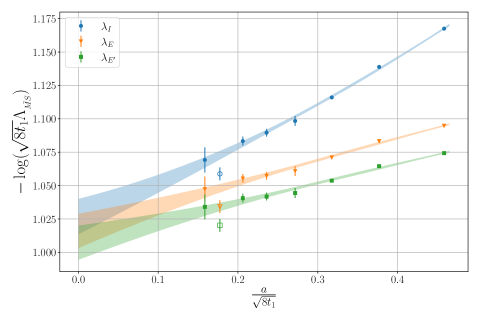
where the separate factors can easily calculated in perturbation theory and are reported in Tab. 2. Now using Eq. (3) truncated to order and fixing in terms of we can determine this quantity in units of from each of our values of and from all of the improved couplings. The result is displayed in Fig. 4. Obviously, a perfect asymptotic scaling would mean that all the values obtained were the same. However, it is natural to expect deviations coming from higher order perturbative and non-perturbative corrections to Eq. (3). These corrections should nonetheless vanish as we approach the continuum limit (). This seems to be the case for our data since the larger difference obtained when comparing with approaches zero as we move towards smaller values of the lattice spacing. To give an estimate we perform a linear plus quadratic extrapolation in for each of the improved couplings separately displayed by the coloured bands in Fig. 4. The extrapolated values of in units of are , and for , and , respectively. Notice that the three values are consistent within errors. The of the fits is not good but this is due entirely to the result at which is seen to deviate considerably from the others. We attribute this phenomenon to a bad estimate of the error based on the large autocorrelation times of the data at this value. A similar phenomenon has been observed and reported in similar studies of the flow in the literature [14, 15]. Our final results having good have been obtained by excluding the value at , but the extrapolated values do not change significantly if we include it. A more detailed analysis of this behaviour will be covered in a future publication [3].
To quote a final estimate of the -parameter for the Yang-Mills theory at large- in the scheme, we give the mean values between the previous results and assign the dispersion as a systematic error.
| (11) |
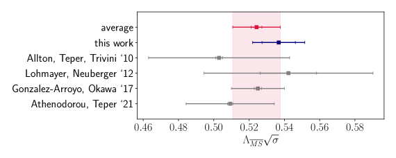
Notice that the use of the flow scale allows one to obtain an estimate at the level of 1-2 per cent. In the previous formula, we also report the final value in units of using the dimensionless ratio that we found in the previous section. For the systematic error, we have added in quadrature the systematic uncertainty on and the one on . Although this other estimate implies a loss in precision, it has the advantage of allowing a comparison with previous determinations. These are in [11] and with the result in the TEK model from [10] and also with the number of given in [16] and from [17]. To collect and compare visually all these results we plot all the values in Fig. 5 in a FLAG-style plot.
4 Conclusions
We used volume reduction to study large Yang-Mills theory by simulating the TEK reduced model. This study focuses on testing predictions of asymptotic scaling for the evolution of the scale of the theory. We performed simulations for and for 8 values of the coupling and obtained a precise determination of the scale. Our study shows consistent results using different improved couplings, having small corrections and allowing a precise determination of the Lambda parameter of the theory in the scheme. Our work is part of a more extensive study to appear in a future publication [3].
References
- [1] A. Hasenfratz, P. Hasenfratz, "The connection between the parameters of lattice and continuum QCD", Phys. Lett. B 93 (1980)
- [2] A. González-Arroyo, C. P. Korthals Altes, "Asymptotic freedom scales for any single plaquette action", Nucl. Phys. B 205 (1), 46-76.
- [3] P. Butti, A. Gonzalez-Arroyo, "Asymptotic scaling in Yang-Mills theory at large-", to appear
- [4] A. González-Arroyo, and M. Okawa, "Twisted-Eguchi-Kawai model: A reduced model for large- lattice gauge theory", Phys. Rev. D 27 (1983)
- [5] A. González-Arroyo and M. Okawa, "A twisted model for large- lattice gauge theory", Phys. Lett. B 120 (1983)
- [6] M. Lüscher, "Properties and uses of the Wilson flow in lattice QCD", JHEP 08 (2010).
- [7] P. Butti, M. García Pérez, A. González-Arroyo, K.I. Ishikawa, and M. Okawa, "Scale setting for large- SUSY Yang-Mills on the lattice", JHEP 07 (2022)
- [8] M. García Pérez, A. González-Arroyo, L. Keegan and M. Okawa, "The twisted gradient flow running coupling", JHEP 01 (2015)
- [9] P. Butti, “Gauge theories with dynamical adjoint fermions at large- on the lattice”, Ph.D. thesis; Univ. Autonoma de Madrid (2023)
- [10] A. González-Arroyo and M. Okawa, "The string tension from smeared Wilson loops at large N", Phys. Lett. B 718 (2013)
- [11] C. Allton, M. Teper, A. Trivini, "On the running of the bare coupling in lattice gauge theories", JHEP 07 (2008)
- [12] G. Parisi, "Recent progresses in gauge theories, in High energy physics", AIP (1981), LNF-80-52-P.
- [13] R. G. Edwards, U. M. Heller, T. R. Klassen, "Accurate scale determinations for the Wilson gauge action", Nucl. Phys. B 517 (1998)
- [14] A. Hasenfratz, C. T. Peterson, J. van Sickle and O. Witzel, " parameter of the SU(3) Yang-Mills theory from the continuous function", Phys. Rev. D 108 (2023)
- [15] K.I. Ishikawa, I. Kanamori, Y. Murakami, A. Nakamura, M. Okawa, R. Ueno, "Non-perturbative determination of the -parameter in the pure SU(3) gauge theory from the twisted gradient flow coupling", JHEP 12 (2017)
- [16] A. Athenodorou, M. Teper, "SU(N) gauge theories in 3+1 dimensions: glueball spectrum, string tensions and topology", JHEP 12 (2021)
- [17] R. Lohmayer, H. Neuberger, “Rectangular Wilson Loops at Large ”, JHEP 08 (2012) 102