Balancing Summarization and Change Detection
in Graph Streams

Abstract

This study addresses the issue of balancing graph summarization and graph change detection. Graph summarization compresses large-scale graphs into a smaller scale. However, the question remains: To what extent should the original graph be compressed? This problem is solved from the perspective of graph change detection, aiming to detect statistically significant changes using a stream of summary graphs. If the compression rate is extremely high, important changes can be ignored, whereas if the compression rate is extremely low, false alarms may increase with more memory. This implies that there is a trade-off between compression rate in graph summarization and accuracy in change detection. We propose a novel quantitative methodology to balance this trade-off to simultaneously realize reliable graph summarization and change detection. We introduce a probabilistic structure of hierarchical latent variable model into a graph, thereby designing a parameterized summary graph on the basis of the minimum description length principle. The parameter specifying the summary graph is then optimized so that the accuracy of change detection is guaranteed to suppress Type I error probability (probability of raising false alarms) to be less than a given confidence level. First, we provide a theoretical framework for connecting graph summarization with change detection. Then, we empirically demonstrate its effectiveness on synthetic and real datasets.

I Introduction

I-A Purpose of This Paper

This study addresses the issue of the extent to which a graph stream should be compressed to detect important changes in it. Recently, it is not uncommon to observe large-scale graphs. Therefore, it is necessary to extract essential information from such massive graphs to detect the changes. Graph summarization is a promising approach for summarizing important attributes or parts of a graph as well as a graph stream [1]. The compressed graph thus obtained is called a summary graph. The more compressed the original graphs are, the better it is in saving computational complexity and space complexity. Although graph summarization provides a concise representation, detecting the intrinsic changes in that stream accurately and reliably is complicated.

In Fig. 1, original and summary graphs are shown at consecutive time points. Here, detecting the changes in the summary graphs is of interest.

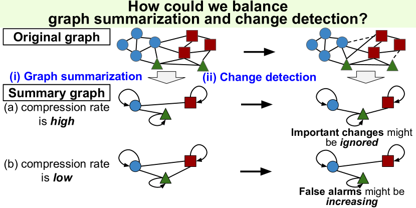
Figure 1: The issue of balancing graph summarization and change detection. An original graph is summarized into a summary graph. (a) when the compression rate is too high, important changes might be ignored. (b) when the compression rate is too low, false alarms of change might increase.

We note that changes detected using summary graphs depend on compression rate of the summary graphs. Here, the compression rate refers to how compactly the original graph is summarized. When the compression rate is excessively high, that is, the original graph is compactly summarized, important changes may be overlooked. By contrast, when the compression rate is extremely low, that is, the original graph is poorly summarized, false alarms may increase because of the detailed changes detected, such as changes of connectivity between nodes. Therefore, there is a trade-off between compression rate of graph summarization and accuracy of graph change detection. Thus, the research question is summarized as follows: How can we balance summarization and change detection from a graph stream? The purpose of this paper is to formulate this issue, and then to propose an algorithm from an information-theoretic perspective.

I-B Related Work

I-B1 Graph Summarization for Graph Streams

Many studies have proposed graph summarization algorithms for a static graph as well as a graph stream [1]. Graphscope [2] detects changes in encoding the cost of a graph segment. Com² [3] finds temporal edge-labelled communities in a graph using tensor decomposition with the minimum description length (MDL) principle [4]. TimeCrunch [5] finds graph structures with MDL using five vocabularies of graph structures and five temporal patterns. NetCondense [6] summarizes a dynamic network by aggregating nodes and time pairs. DSSG [7] identifies six atomic changes by combining the maximum entropy principle and MDL. However, none of these directly addresses the extent to which the original graphs should be summarized to detect significant changes in graph streams.

I-B2 Change Detection in Graph Streams

Change detection in graph streams has been extensively explored [8, 9]. Most of the previous studies addressed parameter changes in data distributions, such as (quasi-)distance-based methods [10, 11] and spectrum-based methods [12, 13, 14]. DeltaCon [15] detects anomalies based on (dis)similarity between successive graphs. An online probabilistic learning framework [16] combines a generalized hierarchical random graph model with a Bayesian hypothesis test. LAD [17] is a Laplacian-based change detection algorithm. HCDL [18] detects hierarchical changes in latent variable models with MDL.

I-C Significance and Novelty

1. Formulation for Balancing Summarization and Change Detection: We formulate the issue of balancing summarization and change detection in a graph stream. Thus far, graph summarization and change detection have been developed independently. To the best of our knowledge, our study is the first attempt.

2. Novel Balancing Algorithm: We propose a novel algorithm called the balancing summarization and change detection algorithm (BSC). The key idea of BSC is to introduce a hierarchical latent variable model and to design a parameterized summary graph based on MDL [4]. With MDL, it is possible to decompose and combine code-lengths at different layers of variables of graphs, such as membership (blocks) of nodes, (super)edges between the blocks, and edges in the original graph. The parameter specifying the summary graph is optimized so that the accuracy of change detection is guaranteed theoretically. This approach is related to [18, 19]. However, HCDL [18] only detects hierarchical changes in latent variable models for data streams and does not consider further compression of summary graphs, whereas the hierarchical latent variable probabilistic model [19] only summarizes a static graph and does not consider further compression nor change detection in an online setting.

3. Empirical Demonstration of the Effectiveness of the Proposed Algorithm: We demonstrate the effectiveness of BSC empirically on synthetic and real datasets. We show that BSC takes an advantage over existing graph summarization algorithms, and is superior or comparable to change detection algorithms.

II Problem Setting

This section presents a probabilistic framework for graph summarization and graph change detection prior to formulating the balancing issue within this framework.

II-A Summary Graph

Let $G=(V,E)$ be a directed graph, where $V$ and $E$ denote a set of nodes and a set of edges, respectively. A summary graph $\bar{G}$ is defined as a triplet $\bar{G}=(S,U,\omega)$, where $S$ is a set of sets of nodes, $U$ is a set of sets of edges, and $\omega$ is an weight function [20]. $S$ is distinct and exhaustive subsets of $V$, i.e., $\bigcup_{A\in S}A=V$ and $\forall A\neq B\in S,A\cap B=\emptyset$. An element in $S$ is called a supernode, and an element in $U$ is called a superedge. We assume that each node in $V$ belongs to a single supernode in $S$. The weight function $\omega$ maps a superedge in $U$ onto a nonzero number. $U$ depends on how the graph is summarized, Typically, it is the total number of edges between supernodes [20].

II-B Probabilistic Model of Graph Summarization

Let $N$ be the number of nodes; $N=|V|$. Let ${\mathcal{K}}$ be a set of numbers of supernodes (blocks) in summary graphs and $K$ be the number of supernodes belonging to $\mathcal{K}$. We introduce three random variables; $X=(x_{ij})\in\{0,1\}^{N\times N}$ is a random variable indicating the connections between nodes. $Z=(z_{k})\in\{0,1\}^{N}$ is a random variable indicating the membership of each node corresponding to a supernode. $Y=(y_{\ell m})\in\{0,1\}^{K\times K}$ is a random variable indicating a superedge connecting supernodes. Let $x,y,z$ denote the realizations of $X,Y,Z$, respectively; $Y$ and $Z$ are considered as latent variables. We formulate the probabilistic model for a graph with latent variables as follows:

$$p(X,Y,Z;\phi,K) \mathrel{\overset{\makebox[0.0pt]{\mbox{\tiny def}}}{=}}p(X|Y,Z;\eta,K)p(Y|Z;\rho,K)p(Z;\xi,K),$$ (1)

where $\phi=(\eta,\rho,\xi)$ is a set of parameters; $\eta\in[0,1]^{K\times K}$, $\rho\in[0,1]$ are parameters of the Bernoulli distributions, and $\xi=(\xi_{1},\dots,\xi_{K})^{\top}\in[0,1]^{K}$ is the one of the categorical distribution, where $\sum_{k=1}^{K}\xi_{k}=1$. The generative model is as follows:

$$x_{ij} \sim\mathrm{Bernoulli}(x_{ij}|y_{z_{i}z_{j}},z_{i},z_{j};\eta,k),$$

$$y_{z_{i}z_{j}} \sim\mathrm{Bernoulli}(y_{z_{i}z_{j}}|z_{i},z_{j};\rho,k),$$

$$z_{i} \sim\mathrm{Categorical}(z_{i};\xi,k).$$ (2)

The random binary variable $y=(y_{\ell m})$ indicates whether a superedge exists between the supernodes $\ell$ and $m$ in a summary graph. The latent variable model in (2) can be thought of as an extension of the stochastic block model (SBM).

Definition II.1.

(Summary graph with hierarchical latent variable model) [19] A summary graph $\bar{G}$ of a graph $G$ in (2) is defined as $\bar{G}=(S,U,\eta,\rho,\xi)$. $S$ and $U$ are the same as those in Sec. II-A, and $\eta$, $\rho$, and $\xi$ are parameters in (2).

II-C Balancing of Summarization and Change Detection

Suppose that we obtain a sequence of graphs $G_{1},G_{2},\dots.$ Then, let us consider the following two issues: 1) graph summarization and 2) graph change detection.

Graph summarization obtains a summary graph $\bar{G}_{t}$ of an original graph $G_{t}$ at each time $t$. Based on the MDL principle [4], the goodness of the summary graph is evaluated with code-length. That is, a summary graph should be chosen so that the total code-length for encoding the original graph as well as the summary graph is as short as possible. Let $\lambda\in\mathbb{R}^{+}$, given a graph $G_{t}$, find a summary graph such that,

$$\min_{\bar{G}_{t}}\{L(G_{t}|\bar{G}_{t})+L_{\lambda}(\bar{G}_{t})\},$$ (3)

where $L(G_{t}|\bar{G}_{t})$ is the code-length of $G_{t}$ for a given $\bar{G}_{t}$, and $L_{\lambda}(\bar{G}_{t})$ is the one of $\bar{G}_{t}$. We design $\lambda$ so that the compression rate would be controlled by $\lambda$, as explained in Sec. III-B.

Graph change detection determines whether an intrinsic change in a sequence of summary graphs occurs at $t$. We employ the MDL principle again to measure how likely an intrinsic change happens, in terms of code-length. More specifically, with the same parameter $\lambda$ as in graph summarization, at $t$, we consider the following statistic:

$$\Phi_{t}=L_{\lambda}(\bar{G}_{t}\oplus\bar{G}_{t-1})-\{L_{\lambda}(\bar{G}_{t})+L_{\lambda}(\bar{G}_{t-1})\},$$ (4)

where $L_{\lambda}(\bar{G}_{t}\oplus\bar{G}_{t-1})$ is the code-length for the concatenation of $\bar{G}_{t}$ and $\bar{G}_{t-1}$, letting them have an identical probabilistic structure. The quantity (4) measures the degree of change in the reduction of the total code-length by separating the graph sequence at $t$. We refer to (4) as the MDL change statistic [21, 22]. Let $\epsilon_{\lambda}(>0)$ be a decision parameter dependent on $\lambda$. We determine that an intrinsic change occurs at $t$ if

$$\Phi_{t}>\epsilon_{\lambda},$$ (5)

otherwise, we determine that a change does not occur. We call this the MDL change test. $\epsilon_{\lambda}$ should be chosen so that the reliability of change detection is theoretically guaranteed as in Sec. III-B.

It should be noted that an intrinsic change is distinguished from a change in appearance. The former refers to a statistically meaningful change, whereas the latter refers to a change of details, including the values of the parameters and the number of edges. Therefore, a change in the appearance does not necessarily indicate an intrinsic change.

The issues of graph summarization and change detection are closely related through $\lambda$. We may design $\lambda$ so that the larger $\lambda$ is, that is, the higher the compression rate is, the smaller $\epsilon_{\lambda}$ is. Eventually, the threshold for change detection can be further relaxed. The $\lambda$ having such a property, is called the balancing parameter. As the parameter varies, the concern is mainly on how compactly the original graph can be summarized to make the performance of change detection in the summary graph sequence as high as possible. This is our main concern for the balancing issue. The concrete design of $\lambda$ and code-length for (3) and (4) are described in Sec. III.

III The Proposed Method: The BSC Algorithm

This section presents the overall flow of BSC, focusing on the basic idea and resulting formulas. Detailed formulation and derivations are provided in the supplementary material.

III-A Code-length for Graph Summarization

We formulate the two code-lengths in (3), where $L(G_{t}|\bar{G}_{t})$ is the code-length of the original graph $G_{t}$ for a given summary graph $\bar{G}_{t}$, and $L_{\lambda}(\bar{G}_{t})$ is the code-length of $\bar{G}_{t}$.

First, we consider $L_{\lambda}(\bar{G}_{t})$. The summary graph $\bar{G}_{t}$ is specified by the latent variables $y_{t}$, $z_{t}$, and the number of blocks $k_{t}$. Therefore, it is necessary to consider the code-length required for encoding $y_{t}$ and $z_{t}$. We hierarchically encode (i) the number of groups $k_{t}$ in the summary graph, (ii) $z_{t}$, and (iii) $y_{t}$ given $z_{t}$, and then sum up the three code-lengths. Specifically, $L_{\lambda}(\bar{G}_{t})$ is defined as

$$L_{\lambda}(\bar{G}_{t}) \mathrel{\overset{\makebox[0.0pt]{\mbox{\tiny def}}}{=}}L_{\mathbb{N}}(k_{t})+L_{\mathrm{NML}}(z_{t};k_{t})+L_{\mathrm{LNML}}(y_{t}|z_{t};\lambda,k_{t}),$$ (6)

where the three terms are code-lengths of (i), (ii), and (iii), respectively. $L_{\mathbb{N}}$ is the optimal code-length for positive integers  [23]: $L_{\mathbb{N}}(k)=2.865+\log{k}+\log{\log{k}}+\dots$, where the sum is taken over positive terms. $L_{\mathrm{NML}}$ is the normalized maximum likelihood (NML) code-length [23] and $L_{\mathrm{LNML}}$ is the luckiness NML (LNML) code-length [24]. NML code-length achieves the minimax regret [4] and is defined as

$$L_{\mathrm{NML}}(z;k) \mathrel{\overset{\makebox[0.0pt]{\mbox{\tiny def}}}{=}}-\log{p(z;\hat{\xi}(z),k)}+\log{\sum_{z^{\prime}}p(z^{\prime};\hat{\xi}(z^{\prime}),k)}$$ (7)

$$=-\sum_{k^{\prime}}n_{k^{\prime}}\log{\frac{n_{k^{\prime}}}{N}}+\log{C_{Z}(k)},$$ (8)

where $\hat{\xi}(z)$ is the maximum likelihood estimator (MLE) given $z$, $n_{k}$ is the number of nodes in the $k$-th block, and $\log{C_{Z}(k)}$ is the parametric complexity for the categorical distribution:

$$\log{C_{Z}(k)}=\log{\sum_{z^{\prime}}p(z^{\prime};\hat{\xi}(z^{\prime}),k)}.$$ (9)

$C_{Z}(k)$ is computable with $O(N+k)$ using a recursive formula  [25]. LNML code-length is defined as follows:

$$L_{\mathrm{LNML}}(y|z;\lambda,k) \mathrel{\overset{\makebox[0.0pt]{\mbox{\tiny def}}}{=}}-\log{p(y|z;\hat{\rho}(y,z),k)\pi(\hat{\rho}(y,z);\lambda)}$$ (10)

$$\quad+\log{C_{Y|Z}(k,\lambda)},$$ (11)

where $\pi(\rho;\lambda)$ denotes the prior distribution of $\rho$. We set $\pi(\rho;\lambda)$ to the beta distribution: $\pi(\rho;\lambda)=\frac{\Gamma(a+b+\lambda)}{\Gamma(a)\Gamma(b+\lambda)}\rho^{a-1}(1-\rho)^{b+\lambda-1}$, where $\Gamma$ denotes the gamma distribution. The second term in (11) is also referred to as the parametric complexity:

$$\log{C_{Y|Z}(k,\lambda)} \mathrel{\overset{\makebox[0.0pt]{\mbox{\tiny def}}}{=}}\log{\sum_{y^{\prime}}p(y^{\prime}|z;\hat{\rho}(y^{\prime},z),k)\pi(\hat{\rho}(y^{\prime},z);\lambda)}.$$ (12)

Next, we consider $L(G_{t}|\bar{G}_{t})$. The original graph $G_{t}$ is specified by $x_{t}$ for given $y_{t}$, $z_{t}$, and $k_{t}$. Let $y_{t}=(y_{\ell m})$, where $y_{\ell m}$ denotes each superedge in the summary graph. Then, we consider the following two cases: (i) $y_{\ell m}=1$ (ii) $y_{\ell m}=0$. For case (i), the hierarchical structure of $x_{t}$, $y_{t}$, $z_{t}$, and $k_{t}$ in (2) holds. The code-length required for encoding $x_{\ell m}^{+}=\{x_{ij}:y_{\ell m}=1,z_{i}=\ell,z_{j}=m\}\subset x_{t}$ for given $y_{t}$, $z_{t}$, and $k_{t}$ is NML code-length for the Bernoulli distribution:

$$L_{\mathrm{NML}}(x_{\ell m}^{+}|y_{\ell m}=1,z_{t};k_{t})=$$ (13)

$$-\log{\prod_{(i,j);z_{i}=\ell,z_{j}=m}p(x_{ij}|y_{\ell m}=1,z_{i}=\ell,z_{j}=m;k_{t})}$$ (14)

$$+\log{\sum_{\{x^{\prime}_{ij}\}}\prod_{(i,j);z_{i}=\ell,z_{j}=m}p(x^{\prime}_{ij}|y_{\ell m}=1,z_{i}=\ell,z_{j}=m;k_{t})}.$$ (15)

The second term in (15) means the parametric complexity of the Bernoulli distribution.

Next, for case (ii), the hierarchical structure of $x_{t}$ for given $y_{t}$, $z_{t}$, and $k_{t}$ does not hold because the corresponding superedge does not exist. Therefore, we adopt a different encoding scheme. Let us denote $x_{\ell m}^{-}=\{x_{ij}:y_{\ell m}=0,z_{i}=\ell,z_{j}=m\}\subset x_{t}$. The key concept is to encode the total possible number of edges in the original graph and the number of configurations for existing edges. The code-length required for encoding it is so-called the counting code-length [24]:

$$\log{(n_{\ell m}+1)}+\log{\begin{pmatrix}n_{\ell m}\\ n_{\ell m}^{+}\end{pmatrix}},$$ (16)

where $n_{\ell m}$ is the total possible number of edges in the original graph between supernodes $\ell$ and $m$, and $n_{\ell m}^{+}$ is the one of existing edges.

By combining (15) and (16), we formulate $L(G_{t}|\bar{G}_{t})$:

$$L(G_{t}|\bar{G}_{t}) \mathrel{\overset{\makebox[0.0pt]{\mbox{\tiny def}}}{=}}L(x_{t}|y_{t},z_{t};k_{t})$$ (17)

$$\mathrel{\overset{\makebox[0.0pt]{\mbox{\tiny def}}}{=}}\sum_{\ell,m}\biggl{\{}y_{\ell m}L_{\mathrm{NML}}(x_{\ell m}^{+}|y_{\ell m}=1,z_{t};k_{t})$$ (18)

$$+(1-y_{\ell m})\left(\log{(n_{\ell m}+1)}+\log{\begin{pmatrix}n_{\ell m}\\ n_{\ell m}^{+}\end{pmatrix}}\right)\biggr{\}}.$$ (19)

The optimization problem of estimating $\bar{G}_{t}$ is converted into

$$\min_{\bar{G}_{t}}\left\{L(G_{t}|\bar{G}_{t})+L_{\lambda}(\bar{G}_{t})\right\}$$ (20)

$$=\min_{k_{t},y_{t},z_{t}}\Bigl{\{}L(x_{t}|y_{t},z_{t};k_{t})+L_{\mathbb{N}}(k_{t})+L_{\mathrm{NML}}(z_{t};k_{t})$$ (21)

$$\quad\quad\quad\quad\quad+L_{\mathrm{LNML}}(y_{t}|z_{t};\lambda,k_{t})\Bigr{\}}.$$ (22)

Given a set of the numbers of supernodes $\mathcal{K}$, for each $k_{t}\in\mathcal{K}$, we obtain $\hat{z}_{t}$ by estimating the block structures and parameter $\hat{\xi}_{t}$ of SBM. We determine $y_{\ell m}=1$ if NML code-length for encoding $x_{\ell m}^{+}$ is shorter than the counting code-length in (19), and $y_{\ell m}=0$ otherwise. Finally, we sum up the four code-lengths, and then select $\hat{k}_{t}\in\mathcal{K}$ with the minimum code-length.

III-B Change Detection

We consider the formulation of (4) and the threshold parameter $\epsilon_{\lambda}$ in (5). First, $L_{\lambda}(\bar{G}_{t}\oplus\bar{G}_{t-1})$ in (4) is defined as

$$L_{\lambda}(\bar{G}_{t}\oplus\bar{G}_{t-1})\mathrel{\overset{\makebox[0.0pt]{\mbox{\tiny def}}}{=}}$$ (23)

$$\quad L_{\mathbb{N}}(k^{\oplus})+L_{\mathrm{NML}}(z_{t};k^{\oplus})+L_{\mathrm{LNML}}(y_{t}|z_{t};\lambda,k^{\oplus})$$ (24)

$$\quad+L_{\mathbb{N}}(k^{\oplus})+L_{\mathrm{NML}}(z_{t-1};k^{\oplus})+L_{\mathrm{LNML}}(y_{t-1}|z_{t-1};\lambda,k^{\oplus}),$$ (25)

where $k^{\oplus}$ denotes the optimal number of blocks. The first three terms refer to the code-lengths to encode $\bar{G}_{t}$ and the last three terms refer to the ones to encode $\bar{G}_{t-1}$.

Next, we consider the threshold determination for the change score $\Phi_{t}$, to raise an alarm for a change point in hypothesis testing. The evaluation metrics are Type I and II error probabilities; Type I error probability leads to a false alarm, whereas Type II one leads to overlooking a change point. We provide the upper bounds on Type I and II error probabilities in the supplementary material. Focusing on Type I error probability, a threshold $\epsilon_{\lambda}$ is specified so that Type I error probability is upper-bounded by a confidence parameter $\delta$. Based on the upper bound of Type I error probability, we have the following theorem for the lower bound of $\epsilon_{\lambda}$.

Theorem III.1.

Let $\epsilon_{\lambda}$ be the threshold for the MDL change test. For a balancing parameter $\lambda\in\mathbb{R}^{+}$, and confidence parameter $0<\delta<1$, $\epsilon_{\lambda}$ satisfies the following inequality:

$$\quad\quad\epsilon_{\lambda}\geq\log{C_{Y|Z}(\lambda,k_{0})C_{Z}(k_{0})}+\frac{L_{\mathbb{N}}(k_{0})-\log{\delta}}{2},$$ (26)

where $k_{0}$ is the true number of blocks. Type I error probability does not exceed $\delta$. Here, $\log{C_{Y|Z}(\lambda,k_{0})}$ and $\log{C_{Z}(k_{0})}$ are the parametric complexities in (12) and (9), respectively.

The relationship between $\lambda$ and $\epsilon_{\lambda}$ represents a trade-off between compression rate of graph summarization and accuracy of change detection. Fig. 2 illustrates the dependence of the parametric complexity on $k$ and $\lambda$. For a fixed $k$, the larger $\lambda$ is (a high compression rate), the smaller the parametric complexity is, which leads to lower $\epsilon_{\lambda}$. In fact, it is not enough to evaluate only Type I error probability. In Sec. IV, we empirically evaluate the relationship between $\lambda$ and Type I / II error probabilities.

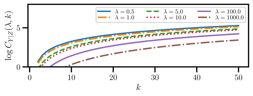
Figure 2: The dependence of the parametric complexity $\log{C_{Y|Z}(\lambda,k)}$ on $k$ and $\lambda$. The parameters of the beta distribution are set to $(a,b)=(0.5,0.5)$.

III-C Overall Flow of BSC Algorithm

In summary, the overall flow of BSC is presented in Algorithm 1. The computational cost of BSC is evaluated as follows: for a fixed $k\in\mathcal{K}$, the computational cost of inference for SBM depends on the algorithm used. In this study, we use the MCMC-based method [26]; the computational cost is $O(N\log^{2}{N})$. Then, the computational cost for calculating the code-lengths in (22) is $O(N+k)$ for $L_{\mathrm{NML}}(z_{t};k_{t})$ and at most $O(|E|)$ for $L(x_{t}|y_{t},z_{t};k_{t})$. Therefore, the total computational cost for fixed $k$ is $O(N\log^{2}{N}+k+|E|)$. In total, the computational cost for the set $\mathcal{K}$ and the total time steps $T$ in a graph stream is $O(T(|\mathcal{K}|(N\log^{2}{N}+|E|)+\sum_{k\in\mathcal{K}}k))$.

Algorithm 1 Balancing Summarization and Change Detection Algorithm (BSC)

0:  $\delta$: a confidence parameter to control Type I error probability, $\lambda$: penalty parameter  ($\lambda>0$), $\mathcal{K}$: a set of the numbers of supernodes in summary graphs.

0:  

1:  for $t=1,\dots$ do

2:     Receive a graph $G_{t}$ ($=x_{t}$).

3:     Estimate the number of blocks and latent variables $(\hat{k}_{t},\hat{y}_{t},\hat{z}_{t})$ according to (22) with $x_{t}$, where $\hat{k}_{t}$ is selected among $\mathcal{K}$.

4:     Calculate the change statistics $\Phi_{t}$ in (4).

5:     Calculate the threshold $\epsilon_{\lambda}$ as the minimum of the inequality in (26).

6:     if $\Phi_{t}>\epsilon_{\lambda}$ then

7:        Raise an alarm of change for summary graph.

8:     end if

9:  end for

IV Experiments

This section demonstrates the effectiveness of BSC through experiments. All experiments were performed on MacOS 10.15.7 with Intel Core i7 and 16GB memory. The source code is available at https://github.com/s-fuku/bsc.

IV-A Synthetic Dataset

IV-A1 Data

For $t=1,\dots,30$, we generated edges $x_{t}$, where the number of nodes was set to $N=200$. First, $x_{1}$ was drawn from SBM [27] with the parameters $\theta_{x}$, $\theta_{z}$, and model $k$; $\theta_{x}$ is the parameter in the Bernoulli distribution for edges and $\theta_{z}$ is the one in the categorical distribution for the blocks (supernodes) of nodes. $\theta_{x}^{(1)}$ and $\theta_{z}^{(1)}$ were sampled from the beta distribution ($a=b=0.5$) and the Dirichlet distribution ($\alpha=1$), respectively. From $t=2$ to $14$, some edges were regenerated according to $\theta_{x}^{(1)}$ for each combination of supernodes with probability $0.05$. At $t=15$, each element in $\theta_{x}^{(1)}$ changed to $\theta_{x}^{(2)}=\max(\tau,\min(\theta_{x}^{(1)}+u,1-\tau))$, where $u$ is drawn from the uniform distribution between $-0.1$ and $0.1$, and $\tau=0.001$. From $t=16$ to $30$, some edges were regenerated in the same way as before. We set $\delta=0.05$, $k\in\{2$, $3$, $4\}$, and $\lambda\in\{0.5$, $1$, $5\}$.

IV-A2 Algorithms for Comparison

We chose the following two representative graph summarization algorithms with MDL and two graph change detection ones with the highest detection accuracy and relatively light-weight computation.

• TimeCrunch [5] encodes model and data, where the model refers to five connectivity structures and five temporal occurrences. We calculated the code-length for the model as a summary graph at each time and used the absolute difference of it as a change score. We chose the top $m\in\{10,50\}$ structures from the candidate set.

• DSSG [7] outputs subgraph structures as a summary graph formed with six atomic changes. We defined the sum of information contexts of all atomic changes at a time point as a change score. We changed $q$ among $\{0.1$, $0.5\}$, where $q$ is expected probability of a random node in the summary graph.

• DeltaCon [15] calculates similarity of consecutive pair of graphs. We defined the change score as $1-$ similarity.

• Eigenspace-based algorithm [12] outputs an anomaly score at each time and we used it as a change score. We set the window size $w=2$.

IV-A3 Evaluation Metrics

We evaluated algorithms in terms of accuracy of change detection and compression rate of the summary graphs. We said that a change occurred at time $t$ if $s_{t}>\epsilon_{\lambda}$, where $s_{t}$ is a change score, and $\epsilon_{\lambda}$ was determined according to (26). Type I error probability was defined as the ratio of the trials at which an algorithm raises false alarms, whereas Type II error probability was defined as the ratio of the trials at which an algorithm overlooks significant changes:

Type  I  error  prob. $$\mathrel{\overset{\makebox[0.0pt]{\mbox{\tiny def}}}{=}}\frac{|\left\{n:s_{t}^{n}\geq\epsilon\mid t\leq 15-\tau,t\geq 15+\tau\right\}|}{n_{\mathrm{trial}}},$$ (27)

Type  II  error  prob. $$\mathrel{\overset{\makebox[0.0pt]{\mbox{\tiny def}}}{=}}\frac{\left|\{n:s_{t}^{n}<\epsilon\mid 15-\tau<t<15+\tau\}\right|}{n_{\mathrm{trial}}},$$ (28)

where $n_{\mathrm{trial}}$ denotes the number of trials for validation. $n$ refers to the index of the trials, $s_{t}^{n}$ is the change score at trial $n$ and time $t$ according to (4), and $\tau\in\mathbb{N}$ is an allowed window for false alarms and overlooks. We set $n_{\mathrm{trial}}=10$ and $\tau=1$.

The accuracy was also evaluated using the area under the curve (AUC) score, which is often used as a measure of change detection [28, 18]. We first fixed the threshold parameter $\epsilon$ and converted the change scores $\{s_{t}\}$ to binary alarms $\{\alpha_{t}\}$. That is, $\alpha_{t}=\mathbbm{1}~{}(s_{t}>\epsilon)$, where $\mathbbm{1}(s)$ denotes a binary function that takes on the value of 1 if and only if $s$ is true. We defined $T_{\mathrm{b}}$ as the maximum tolerance delay in change detection. We set $T_{\mathrm{b}}=1$. When the actual time of the change was $t^{\ast}$, and detected change points were $\{t_{k}\}_{k=1}^{m}$, we defined the benefit of an alarm at time $t_{k}$: $b(t_{k};t^{\ast})=1-|t_{k}-t^{\ast}|/T_{\mathrm{b}}$   $(0\leq|t_{k}-t^{\ast}|<T_{\mathrm{b}})$, and $0$ otherwise. The number of false alarms was calculated as follows: $n_{\mathrm{fa}}=\sum_{k=1}^{m}\alpha_{t_{k}}\mathbbm{1}(b(t_{k};t^{\ast}))=0$. The AUC was calculated with recall rate of the total benefit $b/\sup_{\epsilon}b$ and false alarm rate $n_{\mathrm{fa}}/\sup_{\epsilon}n_{\mathrm{fa}}$, with $\epsilon$ varying.

For the compression rate of summary graphs, we calculated the average code-lengths at $t=15$.

IV-A4 Results

Table I lists the estimated Type I and II error probabilities, AUCs, and the code-lengths of the summary graphs. Type I and II error probabilities for BSC were lower than $0.1$. Type I error probabilities of TimeCrunch and DSSG were higher than that of BSC, while Type II ones were kept relatively low. This is because TimeCrunch and DSSG detected more subtle changes in edges even when significant changes did not occur. The performance of BSC was superior or comparable to those of the change detection algorithms.

TABLE I: Type I and II error probabilities, AUCs, and code-lengths on the synthetic dataset.

	Type I	Type II	AUC	Code-length
BSC ($\lambda=0.5$)	$\mathbf{0.0}$	$0.1$	$0.95\pm 0.00$	$144.39\pm\;\;\;\;\;\;\;\;\;\;\;\;\;\;\;\;\;\;1.28$
BSC ($\lambda=1$)	$\mathbf{0.0}$	$\mathbf{0.0}$	$\mathbf{1.00\pm 0.00}$	$141.82\pm\;\;\;\;\;\;\;\;\;\;\;\;\;\;\;\;\;\;1.20$
BSC ($\lambda=5$)	$0.1$	$\mathbf{0.0}$	$0.95\pm 0.00$	$\;\;\;\;\;\mathbf{138.53\pm\;\;\;\;\;\;\;\;\;\;\;\;\;\;\;1.20}$
TimeCrunch ($m=50$)	$0.2$	$0.1$	$0.83\pm 0.02$	$4101.18\pm 1656.38$
TimeCrunch ($m=10$)	$0.2$	$0.2$	$0.78\pm 0.05$	$4491.39\pm 1711.23$
DSSG ($q=0.1$)	$0.3$	$0.6$	$0.57\pm 0.00$	$2656.54\pm 1006.08$
DSSG ($q=0.5$)	$0.5$	$0.4$	$0.56\pm 0.00$	$1955.48\pm\;\;\;\;\;\;872.90$
DeltaCon	$\mathbf{0.0}$	$0.1$	$0.95\pm 0.00$	—
Eigenspace-based	$\mathbf{0.0}$	$0.1$	$0.95\pm 0.00$	—

The code-lengths with BSC were shorter than those with TimeCrunch and DSSG. This is because of the nature of BSC that it encodes the original graph structures compactly with the hierarchical latent probabilistic variable model.

IV-B TwitterWorldCup2014 Dataset

We also demonstrated the effectiveness of BSC on the TwitterWorldCup2014 dataset [29]. We constructed entity-entity co-mention graphs on an hourly basis between twitter hashtags from June 1 to July 15 (1,080 time points). The total number of entities is 15,856.

We evaluated BSC, DSSG [7], DeltaCon [15], and Eigenspace-based algorithm [12] in terms of AUC with the maximum tolerance delay $T_{b}=1$ hour. For BSC, we set $k\in\{15$, $20$, $25$, $30$, $35\}$ and $\lambda\in\{1$, $100$, $1000\}$. We searched $q\in\{10^{-3}$, $10^{-5}\}$ for DSSG. We set $w=2$ for the Eigenspace-based algorithm. For evaluation, the 22 events annotated as “High importance events” were selected.

Table II summarizes the performances for the remaining games but the first two ones. The code-lengths were calculated when the events happened in the games, and then they are normalized compared to the ones with $\lambda=100$. BSC was superior to other change detection algorithms, and compressed the original graphs more compactly than DSSG with much less time.

TABLE II: AUCs, relative code-lengths, and computation times on the TwitterWorldCup2014 dataset.

	AUC	Relative Code-length	Computation Time (s)
BSC ($\lambda=1$)	$0.73$	$1.08\pm 0.08$	$873$
BSC ($\lambda=100$)	$\mathbf{0.74}$	$1.00\pm 0.00$	$868$
BSC ($\lambda=1000$)	$0.72$	$\mathbf{0.93\pm 0.03}$	$874$
DSSG ($q=10^{-3}$)	$0.53$	$10.23\pm 0.21$	$187,497$
DSSG ($q=10^{-5}$)	$0.51$	$6.76\pm 0.13$	$167,322$
DeltaCon	$0.68$	—	$\mathbf{288}$
Eigenspace-based	$0.64$	—	$5,288$

V Conclusion

We proposed a new formulation with a novel algorithm called BSC to balance graph summarization and change detection in a graph stream. We introduced the hierarchical latent variable model and efficiently encoded its probabilistic structure with MDL. We also theoretically derived the relationship between two parameters in hypothesis testing: the balancing parameter for reduction of superedges in summary graphs and threshold parameter for change detection in summary graphs. Through this relation, the latter was determined by the former. Experimental results demonstrated the effectiveness of BSC.

References

- [1] Y. Liu, T. Safavi, A. Dighe, and D. Koutra, “Graph summarization methods and applications: a survey,” ACM Computing Surveys, pp. 62:1–62:34, 2018.
- [2] J. Sun, S. Papadimitriou, P. S. Yu, and C. Faloutsos, “Graphscope: parameter-free mining of large time evolving graphs,” in Proc. of KDD, 2007, pp. 687–696.
- [3] M. Araujo, S. Papadimitriou, S. Günnemann, C. Faloutsos, P. Basu, A. S. E. Papalexakis, and D. Koutra, “Com2: fast automatic discovery of temporal (‘comet’) communities,” in Proc. of PAKDD, 2014, pp. 271–283.
- [4] K. Yamanishi, Learning with the Minimum Description Length Principle. Springer Nature, 2023.
- [5] N. Shah, D. Koutra, T. Zou, B. Gallagher, and C. Faloutsos, “TimeCrunch: interpretable dynamic graph summarization,” in Proc. of KDD, 2015, p. 1055–1064.
- [6] B. Adhikari, Y. Zhang, A. Bharadwaj, and B. Prakash, “Condensing temporal networks using propagation,” in Proc. of SDM, 2017, p. 417–425.
- [7] S. Kapoor, D. K. Saxena, and M. v. Leeuwen, “Online summarization of dynamic graphs using subjective interestingness for sequential data,” Data Mining and Knowledge Discovery, pp. 88–126, 2020.
- [8] L. Akoglu, H. Tong, and D. Koutra, “Graph based anomaly detection and description: a survey,” Data Mining and Knowledge Discovery, vol. 29, pp. 626–688, 2015.
- [9] S. Ranshous, S. Shen, D. Koutra, S. Harenberg, and C. Faloutsos, “Anomaly detection in dynamic networks: a survey,” Wiley Interdisciplinary Reviews: Computational Statistics, vol. 7, no. 3, 2015.
- [10] D. V. Hinkley, “Inference about the change-point in a sequence of random variables,” Biometrika, vol. 27, no. 1, pp. 1–17, 1970.
- [11] M. Basseville and I. Nikiforov, Detection of abrupt changes: theory and application. Printice Hall, 1993.
- [12] T. Ide and H. Kashima, “Eigenspace-based anomaly detection in computer systems,” in Proc. of KDD, 2004, pp. 440–449.
- [13] S. Hirose, K. Yamanishi, T. Nakata, and R. Fujimaki, “Network anomaly detection based on eigen equation compression,” in Proc. of KDD, 2009, pp. 1185–1194.
- [14] L. Akoglu and C. Faloutsos, “Event detection in time series of mobile communication graphs,” in Proc. of 27th Army Science Conference, 2010.
- [15] D. Koutra, N. Shah, J. Vogelstein, B. Gallagher, and C. Faloutsos, “DeltaCon: principled massive-graph similarity function with attribution,” ACM Transactions on Knowledge Discovery from Data, vol. 10, no. 3, pp. 28:1–28:43, 2016.
- [16] L. Peel and A. Clauset, “Detecting change points in the large-scale structure of evolving networks,” in Proc. of AAAI, 2015, pp. 2914–2920.
- [17] S. Huang, Y. Hitti, G. Rabusseau, and R. Rabbany, “Laplacian change point detection for dynamic graphs,” in Proc. of KDD, 2020, pp. 349–358.
- [18] S. Fukushima and K. Yamanishi, “Detecting hierarchical changes in latent variable models,” in Proc. of ICDM, 2020, pp. 1128–1134.
- [19] S. Fukushima, R. Kanai, and K. Yamanishi, “Graph summarization with latent variable probabilistic models,” in Proc. of ComplexNetworks, 2021, pp. 428–440.
- [20] K. Lee, H. Jo, J. Ko, S. Lim, and K. Shin, “SSumM: sparse summarization of massive graphs,” in Proc. of KDD, 2020, p. 144–154.
- [21] K. Yamanishi and S. Fukushima, “Model change detection with the MDL principle,” IEEE Transactions on Information Theory, vol. 9, no. 64, pp. 6115–6126, 2018.
- [22] K. Yamanishi and K. Miyaguchi, in Proc. of BigData, 2016, pp. 156–163.
- [23] J. Rissanen, “Modeling by shortest data description,” Automatica, vol. 14, pp. 465–471, 1978.
- [24] P. Grünwald, The minimum description length principle. MIT Press, 2007.
- [25] P. Kontkanen and P. Myllymäki, “A linear-time algorithm for computing the multinomial stochastic complexity,” Information Processing Letters, vol. 103, no. 6, pp. 227–233, 2007.
- [26] T. P. Peixoto, “Efficient monte carlo and greedy heuristic for the inference of stochastic block models,” Physical Review E, vol. 89, p. 012804, 2014.
- [27] T. Snijders and K. Nowicki, “Estimation and prediction for stochastic blockmodels for graphs with latent block structure,” Journal of Classification, vol. 64, no. 4, pp. 583–639, 1997.
- [28] S. Fukushima and K. Yamanishi, “Detecting metachanges in data streams from a viewpoint of MDL,” Entropy, vol. 21, no. 12, p. 1134, 2019.
- [29] S. Rayana and L. Akoglu, “Less is more: building selective anomaly ensembles,” ACM Transactions on Knowledge Discovery from Data, vol. 10, no. 4, pp. 1–33, 2016.