Towards Assessing and Benchmarking Risk-Return Tradeoff of Off-Policy Evaluation

Abstract

Off-Policy Evaluation (OPE) aims to assess the effectiveness of counterfactual policies using only offline logged data and is often used to identify the top-$k$ promising policies for deployment in online A/B tests. Existing evaluation metrics for OPE estimators primarily focus on the “accuracy” of OPE or that of downstream policy selection, neglecting risk-return tradeoff in the subsequent online policy deployment. To address this issue, we draw inspiration from portfolio evaluation in finance and develop a new metric, called SharpeRatio@k, which measures the risk-return tradeoff of policy portfolios formed by an OPE estimator under varying online evaluation budgets ($k$). We validate our metric in two example scenarios, demonstrating its ability to effectively distinguish between low-risk and high-risk estimators and to accurately identify the most efficient estimator. This efficient estimator is characterized by its capability to form the most advantageous policy portfolios, maximizing returns while minimizing risks during online deployment, a nuance that existing metrics typically overlook. To facilitate a quick, accurate, and consistent evaluation of OPE via SharpeRatio@k, we have also integrated this metric into an open-source software, SCOPE-RL. Employing SharpeRatio@k and SCOPE-RL, we conduct comprehensive benchmarking experiments on various estimators and RL tasks, focusing on their risk-return tradeoff. These experiments offer several interesting directions and suggestions for future OPE research.

1 Introduction

Reinforcement Learning (RL) has achieved considerable success in a variety of applications requiring sequential decision-making. Nonetheless, its online learning approach is often seen as problematic due to the need for active interaction with the environment, which can be risky, time-consuming, and unethical (Fu et al., 2021; Matsushima et al., 2021). To mitigate these issues, learning new policies offline from existing historical data, known as Offline RL (Levine et al., 2020), is becoming increasingly popular for real-world applications (Qin et al., 2021). Typically, in the offline RL lifecycle, promising candidate policies are initially screened through Off-Policy Evaluation (OPE) (Fu et al., 2020), followed by the selection of the final production policy from the shortlisted candidates using more dependable online A/B tests (Kurenkov & Kolesnikov, 2022), as shown in Figure 1.

When evaluating the efficacy of OPE methods, research has largely concentrated on “accuracy” metrics like mean-squared error (MSE) (Uehara et al., 2022; Voloshin et al., 2019), rank correlation (rankcorr) (Fu et al., 2021; Paine et al., 2020), and regret in subsequent policy selection (Doroudi et al., 2017; Tang & Wiens, 2021). However, these existing metrics do not adequately assess the balance between risk and return experienced by an estimator during the online deployment of selected policies. Crucially, MSE and rankcorr fall short in distinguishing whether an estimator is underevaluating near-optimal policies or overevaluating poor-performing ones, which influence the risk-return dynamics in OPE and policy selection in different ways. The regret metric solely emphasizes the optimal outcome among the top-$k$ policies selected by OPE, neglecting the potential adverse effects on the environment when implementing suboptimal policies in online A/B testing scenarios.

Contributions.

Aiming for a more informative evaluation-of-OPE, we propose a new evaluation-of-OPE metric called SharpeRatio@k. This metric evaluates both the potential risk and return when deploying the resulting top-$k$ policies in the A/B testing phase. Drawing inspiration from financial portfolio management, we view the shortlisted candidate policies as a policy portfolio formulated by an OPE estimator. This approach allows us to assess the risk, return, and efficiency of an estimator based on the statistics of its policy portfolio. Specifically, we use the Sharpe ratio (Sharpe, 1998) to measure OPE efficiency. A policy portfolio is deemed efficient if it includes policies that substantially enhance the performance of the behavior (data collection) policy (high return), while avoiding inclusion of underperforming policies that could detrimentally affect rewards during A/B testing (low risk). As an initial validation, we showcase in two example scenarios how SharpeRatio@k can discern between high- and low-risk OPE estimators, a distinction not captured by any existing metric.

In addition to developing SharpeRatio@k, we have also implemented this metric in an open-source software named SCOPE-RL (Kiyohara et al., 2023). SCOPE-RL serves as a versatile tool and testing platform for OPE estimators, providing user-friendly APIs and comprehensive insights into the risk-return tradeoff of OPE estimators. Using SharpeRatio@k and SCOPE-RL, we conduct extensive benchmark experiments with various OPE estimators and RL environments, evaluating their risk-return tradeoffs across different online evaluation budgets (i.e., varying $k$ values).

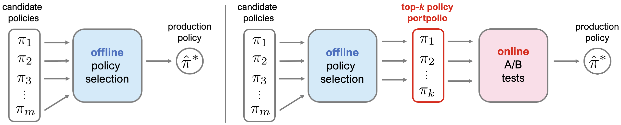
Figure 1: (Left) Conventional (off-)policy selection directly chooses the production policy via OPE. (Right) Practical workflow of policy evaluation and selection involves OPE as a screening process where an OPE estimator ($\hat{J}$) chooses top-$k$ candidate policies that are to be tested in online A/B tests, where $k$ is a pre-defined online evaluation budget. A policy that is identified as the best policy based on the evaluation process will be chosen as the production policy ($\hat{\pi}^{*}$).

Our contributions can be summarized as follows:

• New Evaluation-of-OPE Metric: We have introduced SharpeRatio@k, a novel evaluation metric specifically designed to assess the risk, return, and efficiency of OPE estimators, offering a more comprehensive analysis regarding the evaluation of OPE.

• Benchmarks and Future Directions: Through example scenarios and a range of RL tasks, we demonstrate that SharpeRatio@k is capable of measuring the risk, return, and efficiency of estimators whereas existing metrics fail to do so. We also suggest several future directions for OPE research based on the results that SharpeRatio@k produces.

• Open-Source Implementation: We have developed and integrated SharpeRatio@k into an open-source software named SCOPE-RL. This software is tailored to enable quick, accurate, and insightful evaluation of OPE, enhancing the accessibility and utility of our metric.

2 Off-Policy Evaluation in RL

We consider a general RL setup, formalized by a Markov Decision Process (MDP) defined by the tuple $\langle\mathcal{S},\mathcal{A},\mathcal{T},P_{r},\gamma\rangle$. Here, $\mathcal{S}$ represents the state space and $\mathcal{A}$ denotes the action space, which can either be discrete or continuous. Let $\mathcal{T}:\mathcal{S}\times\mathcal{A}\rightarrow\mathcal{P}(\mathcal{S})$ be the state transition probability, where $\mathcal{T}(s^{\prime}|s,a)$ is the probability of observing state $s^{\prime}$ after taking action $a$ in state $s$. $P_{r}:\mathcal{S}\times\mathcal{A}\times\mathbb{R}\rightarrow[0,1]$ represents the probability distribution of the immediate reward, and $R(s,a):=\mathbb{E}_{r\sim P_{r}(r|s,a)}[r]$ is the expected immediate reward when taking action $a$ in state $s$. $\pi:\mathcal{S}\rightarrow\mathcal{P}(\mathcal{A})$ denotes a policy, where $\pi(a|s)$ is the probability of taking action $a$ in state $s$.

Off-Policy Evaluation (OPE) aims to evaluate the expected reward under an evaluation (new) policy, called the policy value, using only a fixed logged dataset. More precisely, the policy value is defined as the following expected trajectory-wise reward obtained by deploying an evaluation policy $\pi$:

$$J(\pi):=\mathbb{E}_{\tau\sim p_{\pi}(\tau)}\left[\sum_{t=0}^{T-1}\gamma^{t}r_{t}\right],$$

where $\gamma\in(0,1]$ is a discount factor and $p_{\pi}(\tau)=p(s_{0})\prod_{t=0}^{T-1}\pi(a_{t}|s_{t})\mathcal{T}(s_{t+1}|s_{t},a_{t})P_{r}(r_{t}|s_{t},a_{t})$ is the probability of observing a trajectory under evaluation policy $\pi$. The logged dataset $\mathcal{D}$ available for OPE is generated by a behavior policy $\pi_{b}$ (which is different from $\pi$) as

$$\mathcal{D}:=\{(s_{t},a_{t},s_{t+1},r_{t})\}_{t=0}^{T-1}\sim p(s_{0})\prod_{t=0}^{T-1}\pi_{b}(a_{t}|s_{t})\mathcal{T}(s_{t+1}|s_{t},a_{t})P_{r}(r_{t}|s_{t},a_{t}).$$

Given the logged dataset $\mathcal{D}$, the typical goal of OPE is to develop an estimator $\hat{J}(\pi;\mathcal{D})$ that can accurately estimate the true value of $\pi$, i.e., $J(\pi)$. The complexity of OPE arises from the fact that we only have access to logged feedback for actions selected by the behavior policy. This necessitates tackling challenges like counterfactual estimation and distribution shift, both of which can significantly contribute to high bias and variance in estimations (Liu et al., 2018; Thomas et al., 2015) (Appendix A.1 provides a detailed overview of some notable OPE estimators developed to address these specific challenges.).

Practical workflow of policy evaluation and selection.

Due to the presence of bias-variance issues, we cannot exclusively depend on OPE results for selecting a policy for production. Instead, a more practical approach often involves a combination of OPE results and online A/B testing, offering a balance of speed and reliability in policy evaluation and selection (Kurenkov & Kolesnikov, 2022). Specifically, as demonstrated in Figure 1 (Right), this practical approach starts with the elimination of harmful policies using OPE results, followed by A/B testing of the top-$k$ shortlisted policies for a more dependable online assessment. In the following sections, we focus on this practical workflow, aiming to evaluate the effectiveness of OPE estimators in choosing the top-$k$ candidate policies for further assessment in online A/B testing.

Existing evaluation-of-OPE metrics and their issues.

In existing literature, the following three metrics are often used to evaluate and compare the “accuracy” of OPE estimators:

• Mean Squared Error (MSE) (Voloshin et al., 2019): This metric measures the estimation accuracy of estimator $\hat{J}$ among a set of policies $\Pi$ as $(1/|\Pi|)\sum_{\pi\in\Pi}\mathbb{E}_{\mathcal{D}}[(\hat{J}(\pi;\mathcal{D})-J(\pi))^{2}]$.

• Rank Correlation (Rankcorr) (Fu et al., 2021; Paine et al., 2020): This metric measures how well the ranking of candidate policies is preserved in the OPE results and is defined as the spearman’s rank correlation between $\{J(\pi)\}_{\pi\in\Pi}$ and $\{\hat{J}(\pi;\mathcal{D})\}_{\pi\in\Pi}$.

• Regret@$\bm{k}$ (Doroudi et al., 2017): This metric measures how well the best policy among the top-$k$ candidate policies selected by an estimator performs. In particular, Regret@1 measures the performance difference between the true best policy $\pi^{\ast}$ and the best policy estimated by the estimator as $J(\pi^{\ast})-J(\hat{\pi}^{\ast})$ where $\hat{\pi}^{\ast}:={\arg\max}_{\pi\in\Pi}\hat{J}(\pi;\mathcal{D})$.

MSE measures the accuracy of OPE estimation whereas the latter two metrics assess the accuracy of policy selection. By combining these metrics, we can quantify how likely an OPE estimator can choose a near-optimal policy in policy selection (Figure 1 (Left)). However, a significant limitation of these metrics is their failure to assess or acknowledge the potential risk associated with implementing harmful policies, a frequent occurrence in more practical two-stage selection workflow having online A/B tests as a final process (Figure 1 (Right)). For example, in the scenario depicted in Figure 2, all three metrics yield identical evaluations for both estimators X and Y. Yet, with estimator X underestimating the value of near-optimal policies and estimator Y overestimating that of detrimental policies, there is a marked difference in their risk-return tradeoff, which existing metrics overlook by design. This discrepancy underscores the need for a new evaluation-of-OPE metric that can accurately quantify an estimator’s risk-return tradeoff, going beyond mere accuracy assessment.

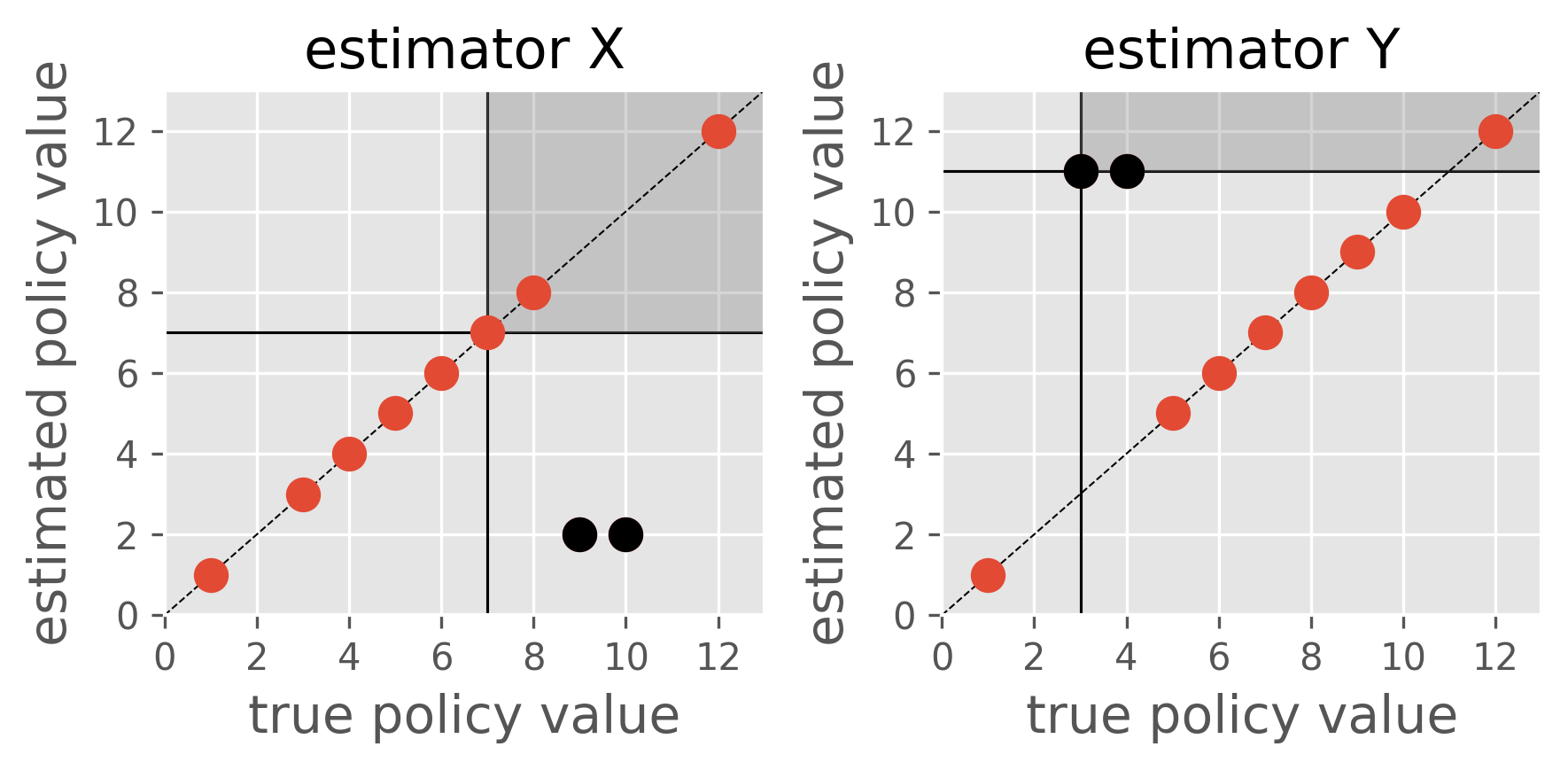
	estimator X	estimator Y
MSE	11.3	11.3
Rankcorr	0.413	0.413
Regret@1	0.0	0.0

Figure 2: A toy example illustrating the situation where existing metrics (MSE, Rankcorr, and Regret) fail to evaluate the risk in the off-policy selection (OPS) task. Both estimators X and Y conduct OPS on the same set of candidate policies. X underestimates the performances of the policies indicated by the black dots while Y overestimates them. The shaded regions show the top-3 policies (policy portfolio) selected by each estimator, indicating that Y is riskier than X since Y includes worse policies in its portfolio. Nonetheless, existing metrics give identical evaluations for X and Y.

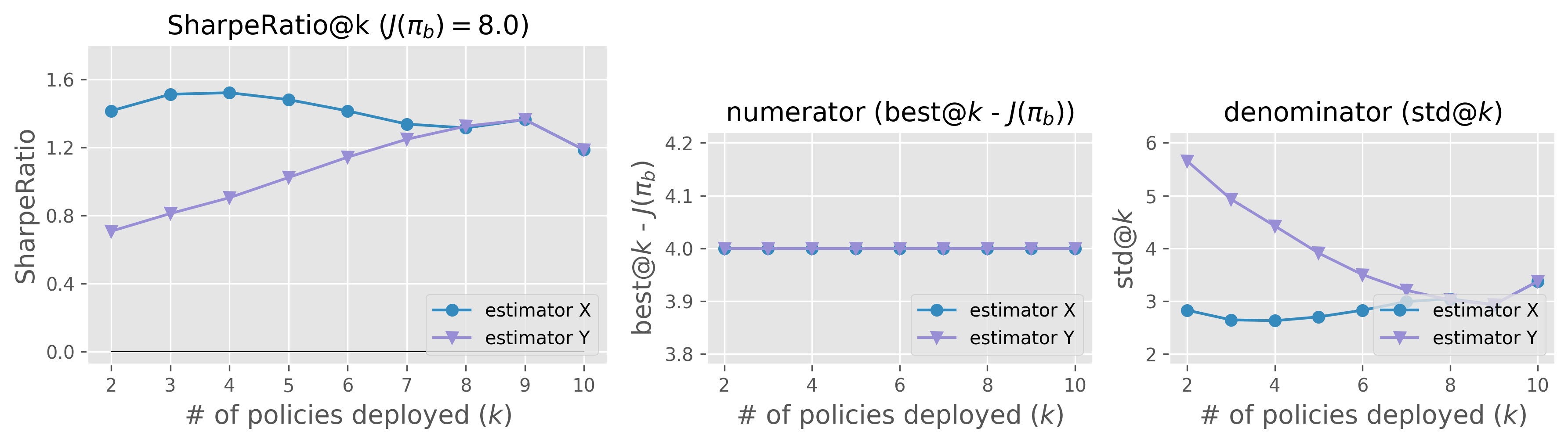
Figure 3: Evaluating estimators X and Y in the toy example of Figure 2 with SharpeRatio@k.

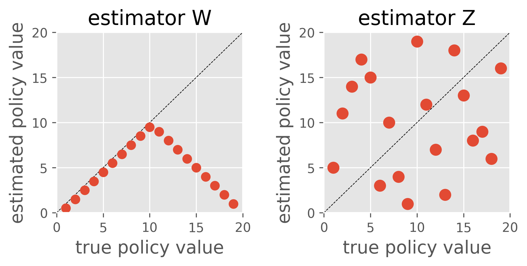
	estimator W	estimator Z
MSE	60.1	58.6
Rankcorr	0.079	0.023
Regret@1	9.0	9.0

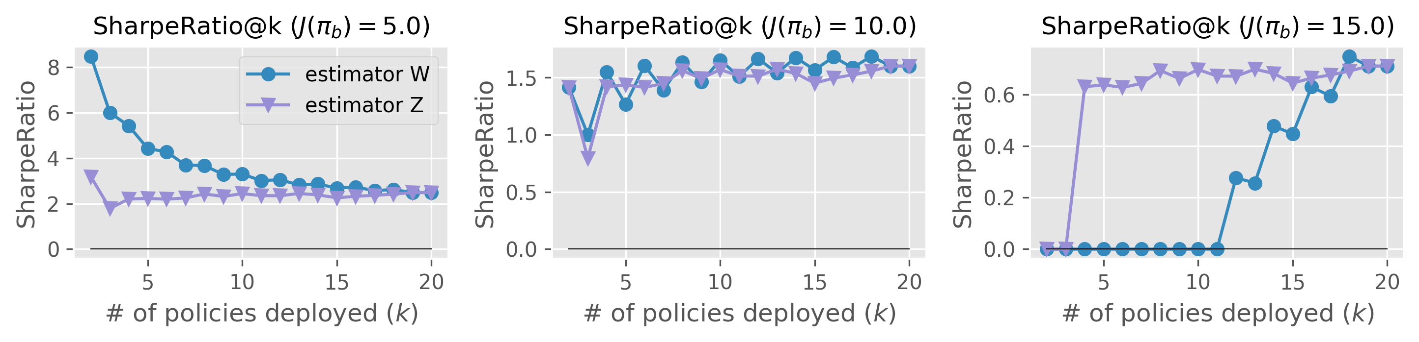
Figure 4: A toy example illustrating the case of evaluating a conservative OPE (estimator W) and uniform random selection (estimator Z) with conventional evaluation-of-OPE metrics (the right top table) and SharpeRatio@k (the bottom figures).

3 Evaluating the Risk-Return Tradeoff in OPE via SharpeRatio@k

Driven by the inadequacy in assessing risk-return tradeoff in existing literature, we introduce a novel evaluation metric for OPE estimators, which we call SharpeRatio@k. This evaluation-of-OPE metric conceptualizes the top-$k$ candidate policies selected by an estimator as its “policy portfolio” inspired by financial risk-return assessments (Connor et al., 2010; Sharpe, 1998).

Note that we include the behavior policy $\pi_{b}$ as one of the candidate policies when computing SharpeRatio@k, and thus it is always non-negative and behaves differently given different $\pi_{b}$.

Our SharpeRatio@k calculates the return (best@$k$) relative to a risk-free baseline ($J(\pi_{b})$), while incorporating risk (std@$k$) in its denominator. Reporting SharpeRatio@k under varying online evaluation budgets, i.e., different values of $k$, is particularly useful to evaluate and understand the risk-return tradeoff of OPE estimators. Below, we showcase how SharpeRatio@k provides valuable insights for comparing OPE estimators in two practical scenarios while the existing metrics fall short.

Scenario 1: Overestimation vs. Underestimation.

The first example is the one illustrated in Figure 2, where current evaluation-of-OPE metrics fail to assess the risk of overestimating the effectiveness of underperforming policies, producing identical values for estimators X and Y. In this context, SharpeRatio@k offers more valuable insights. As evident in Figure 3, it assigns a higher score to estimator X than to Y. To delve into the mechanisms of SharpeRatio@k, we have separately charted its numerator (return) and denominator (risk) in Figure 3. This breakdown of SharpeRatio@k reveals that the return ($\text{best@}k(\hat{J})-J(\pi_{b})$) is identical for both X and Y, but the risk ($\text{std@}k(\hat{J})$) is substantially greater for estimator Y. This is because Y overestimates the value of underperforming policies, thereby increasing the risk of implementing these harmful policies in future online A/B tests. Consequently, in this particular instance, estimator X is a better choice than Y, a distinction that existing metrics utterly fail to recognize.

Scenario 2: Conservative vs. Random.

In our next example, we compare a conservative OPE estimator (estimator W, which consistently underestimates) with a uniform random estimator (estimator Z), as depicted in Figure 4. Similarly to the prior example, the table in Figure 4 indicates that conventional metrics yield nearly the same values for W and Z, despite their distinctly different behaviors. This obscures the selection of the more suitable estimator. SharpeRatio@k excels in identifying a more effective estimator, considering the risk-return tradeoff and the specific problem instance. Specifically, Figure 4 demonstrates how SharpeRatio@k evaluates estimators W and Z under three different behavior policies, each with varying effectiveness ($J(\pi_{b})=5.0,10,15$, where higher values signify more effective behavior policy $\pi_{b}$). The results show that when $\pi_{b}$ is less effective ($J(\pi_{b})=5.0$), SharpeRatio@k favors estimator W for its lower risk. Conversely, with a moderately effective $\pi_{b}$ ($J(\pi_{b})=10$), SharpeRatio@k shows no preference between the two estimators, suggesting their similar efficiencies in this context. Lastly, in scenarios where $\pi_{b}$ is highly effective ($J(\pi_{b})=15$), estimator Z is preferred by SharpeRatio@k due to its higher potential for selecting superior policies compared to $\pi_{b}$. Thus, SharpeRatio@k proves to be a more informative and practical metric than conventional accuracy metrics, providing crucial insights for selecting the most efficient estimator in relation to their risk-return tradeoff.

Open-Source Implementation.

In addition to developing SharpeRatio@k, to facilitate its concise and precise usage in future research and practice, we provide its implementation and examples in SCOPE-RL, an open-source python software for offline RL and OPE (Kiyohara et al., 2023). Our experiments in the following section are also implemented on top of this software.

4 OPE Benchmarks with SharpeRatio@k

This section evaluates typical OPE estimators with SharpeRatio@k and SCOPE-RL, which results in several valuable future directions and recommendations for OPE research.

4.1 Experiment Setting

RL tasks.

We use a total of 7 tasks including Reacher, InvertedPendulum, Hopper, Swimmer (continuous control) from Gym-Mujuco (Brockman et al., 2016; Todorov et al., 2012) and CartPole, MountainCar, Acrobot (discrete control) from Gym-Classic Control (Brockman et al., 2016). Below, we describe the experiment setting for continuous control tasks in detail. A similar procedure is applicable to the discrete control tasks as described in Appendix A.2.

Data Generation.

We initially train a behavior policy using SAC (Haarnoja et al., 2018) in an online environment and then introduce Gaussian noise to induce stochasticity, creating a logged dataset $\mathcal{D}^{(tr)}$ for the offline training of candidate policies. To establish a diverse set of candidate policies ($\Pi$), we train CQL (Kumar et al., 2020) and IQL (Kostrikov et al., 2022), each implemented in d3rlpy (Seno & Imai, 2021), using three distinct neural networks for each method. By adding Gaussian noise with four different standard deviations to each of these trained policies, we generate a total of 24 policies. From this assortment, we randomly select 10 policies for each experiment to form our set of candidate policies ($\Pi$). We conduct OPE simulations based on logged dataset $\mathcal{D}^{(te)}$ with $n=10,000$ trajectories generated under the behavior policy and 10 different random seeds. Note that we report MSE and Regret normalized by the average and maximum policy value among candidate policies, respectively as nMSE and nRegret@1.

4.2 Compared estimators

We evaluate the following estimators using SharpeRatio@k and conventional accuracy metrics. Appendix A.1 provides rigorous definitions and detailed descriptions of these estimators.

Direct Method (DM) (Le et al., 2019): This estimator approximates the Q-function (state-action value) $\hat{Q}(s_{t},a_{t})\approx R(s_{t},a_{t})+\mathbb{E}[\sum_{t^{\prime}=t+1}^{T-1}\gamma^{t^{\prime}-t}r_{t}|s_{t},a_{t},\pi]$ using the logged data and then estimates the policy value based on this estimated Q-function. This estimator can produce high bias when $\hat{Q}$ is inaccurate, while its variance is often small.

Per-Decision Importance Sampling (PDIS) (Precup et al., 2000): Leveraging the sequential structure of the MDP, this estimator corrects the distribution shift between policies by multiplying the importance weights of previous actions at each time step $t$, i.e., $\prod_{t^{\prime}=0}^{t}\frac{\pi(a_{t^{\prime}}|s_{t^{\prime}})}{\pi_{b}(a_{t^{\prime}}|s_{t^{\prime}})}$. This estimator is unbiased, but it suffers from high variance, especially when $T$ is large.

Doubly Robust (DR) (Jiang & Li, 2016; Thomas & Brunskill, 2016): This estimator combines model-based and importance sampling-based approaches. Specifically, it uses DM as a baseline estimation and applies importance sampling only to the residual of the discounted reward. In this way, DR often reduces variance comapred to PDIS while remaining unbiased.

Marginal Importance Sampling (MIS) (Liu et al., 2018; Uehara et al., 2020): This estimator relies on the marginalized importance weight ($\frac{d^{\pi}(s,a)}{d^{\pi_{b}}(s,a)}$) instead of the per-decision importance weights used in PDIS. MIS reduces variance compared to PDIS because the marginal importance weights do not depend on the trajectory length $T$. Marginal Doubly Robust (MDR) is its DR variant.

Note that we use self-normalized importance weights for PDIS, DR, MIS, and MDR to stabilize their estimations and estimate the marginal importance weights by BestDICE (Yang et al., 2020). For DM, DR, and MDR, we use FQE (Le et al., 2019) with a neural network to estimate $Q(s_{t},a_{t})$.

Figure 5: (Left) Comparison of SharpeRatio@4 and conventional metrics (RankCorr, nRegret, nMSE) in evaluation-of-OPE. (Right) The number of trials in which the best estimator, selected by SharpeRatio@4 (SR@4) and conventional metrics, aligns. Both figures report the results of 70 trials, consisting of 7 tasks and 10 random seeds for each. A lower value is better for nMSE and nRegret, while a higher value is better for RankCorr and SharpeRatio@4.

Figure 6: Evaluation-of-OPE results based on SharpeRatio@k (the left figure) and conventional metrics including nMSE, RankCorr, and nRegret@1 (the right three figures) in MountainCar. A lower value is better for nMSE and nRegret@1, while a higher value is better for RankCorr and SharpeRatio@k. The stars ($\star$) indicate the best estimator under each metric.

Figure 7: Reference statistics of the top-$\bm{k}$ policy portfolio formed by each estimator in MountainCar. “best” is used as the numerator of SharpeRatio@k, while “std” is used as its denominator. A higher value is better for “best” and “$k$-th best policy’s performance”, while a lower value is better for “std”. The dark red lines show $J(\pi_{b})$, which is the risk-free baseline of SharpeRatio@k.

4.3 Results

This section discusses key observations in our benchmark experiments. Appendix A.3 provides more comprehensive results and discussion with more RL environments and metrics.

How does SharpeRatio@k behave differently from conventional metrics?

Figure 5 (Left) illustrates the correlation and divergence between SharpeRatio@4 and conventional metrics in evaluating OPE estimators across various RL tasks. Each point in the figure represents the metrics for 5 estimators over 70 trials, consisting of 7 different tasks and 10 random seeds. Figure 5 (Right) presents the number of trials where the best estimators, as identified by SharpeRatio@4 and each conventional metric, coincide. These figures reveal that superior conventional metric values (i.e., higher RankCorr and lower nRegret and nMSE) do not consistently correspond to higher SharpeRatio@4 values. The most significant deviation of SharpeRatio@4 is from nMSE, which is understandable given that nMSE focuses solely on the estimation accuracy of OPE without considering policy selection effectiveness. In contrast, SharpeRatio@4 shows some correlation with policy selection metrics (RankCorr and nRegret). Nonetheless, the best estimator chosen by SharpeRatio@4 often differs from those selected by RankCorr and nRegret. SharpeRatio@4 and nRegret align in only 8 of the 70 trials, and RankCorr, despite being the most closely correlated metric with SharpeRatio, diverges in the choice of the estimator in over 40% of the trials (29 of 70). The following sections explore specific instances where SharpeRatio@k and conventional metrics diverge, demonstrating how SharpeRatio@k effectively validates the risk-return trade-off, while conventional metrics fall short.

SharpeRatio@k is more appropriate and informative than conventional accuracy metrics.

Figure 7 contrasts the benchmark results obtained using SharpeRatio@k with those derived from conventional metrics in the MountainCar task. Figure 7 details reference statistics for the top-$k$ policy portfolios created by each estimator. Notably, the “$k$-th best policy’s performance” indicates how well the policy, ranked $k$-th by each estimator, performs. These results highlight that the preferred OPE estimator varies significantly based on the evaluation metrics used. For instance, MSE and Regret favor MIS as the best estimator, while Rankcorr and SharpeRatio@7 select DM, and SharpeRatio@4 opts for PDIS. Upon examining these three estimators through the reference statistics in Figure 7, it becomes evident that conventional metrics tend to overlook the risk associated with OPE estimators including suboptimal policies in their portfolio. Specifically, nMSE and nRegret fail to recognize the danger of MIS implementing an almost worst-case estimator for $k\leq 4$. Additionally, RankCorr does not acknowledge the risk involved with PDIS implementing a nearly worst-case estimator for $k\leq 6$, and it inappropriately ranks PDIS higher than MDR, which avoids deploying a suboptimal policy until the last deployment ($k=9,10$). In contrast, SharpeRatio@k effectively discerns the varied characteristics of policy portfolios and adeptly identifies a safe and efficient estimator that is adaptable to the specific budget ($k$) and problem instance ($J(\pi_{b})$). Overall, the benchmark findings suggest that SharpeRatio@k offers a more pragmatically meaningful comparison of OPE estimators than existing accuracy metrics.

SharpeRatio@k and benchmark results suggest future research directions.

The benchmarking results of OPE estimators with SharpeRatio@4 provide the following directions and suggestions for future OPE research.

1. Future research should perform evaluation-of-OPE based on SharpeRatio@k: The findings from the previous section suggest that SharpeRatio@k provides more actionable insights compared to traditional accuracy metrics. The benchmark results using SharpeRatio@k often significantly differ from those obtained with conventional accuracy metrics. This highlights the importance of integrating SharpeRatio@k into future research to more effectively evaluate the efficiency of OPE estimators.

2. A new estimator that explicitly optimizes the risk-return tradeoff: While DR and MDR are generally regarded as advanced in existing literature, they do not consistently outperform DM, PDIS, and MIS according to SharpeRatio@k. This is attributable to their lack of specific design for optimizing the risk-return tradeoff and efficiency. Consequently, a promising research avenue would be to create a new estimator that explicitly focuses more on optimizing this risk-return tradeoff than existing methods.

3. A new estimator selection method: The results show that the most efficient estimator varies significantly across different environments, underscoring the need for adaptively selecting the most suitable estimator for reliable OPE. Given that existing estimator selection methods predominantly focus on “accuracy” metrics like MSE and Regret (Lee et al., 2022; Su et al., 2020; Udagawa et al., 2023; Xie & Jiang, 2021; Zhang & Jiang, 2021), there is an intriguing opportunity for future research to develop a novel estimator selection method that considers risks and efficiency.

5 Related Work

Evaluation-of-OPE Metrics

The pursuit of accurately evaluating counterfactual policies has traditionally been a cornerstone of OPE research (Uehara et al., 2022; Saito et al., 2021b). Consequently, the Mean-Squared Error (MSE) has become the go-to “accuracy” metric, with the comprehensive study by Voloshin et al. (2019) exploring how the MSE of OPE estimators varies with trajectory lengths and degrees of distribution shift. In a different approach, Doroudi et al. (2017) highlights instances of biased policy selection caused by OPE and advocates for evaluating estimators based on their capability to identify the most effective policy, aligning with the concept of the regret metric. Subsequent benchmarks (Fu et al., 2021; Tang & Wiens, 2021) have compared estimators on their regret and rank correlation in downstream policy selection, but these metrics remain focused solely on the “accuracy” of policy selection, neglecting the risk-return tradeoff in subsequent A/B tests.

In contrast, SharpeRatio@k brings a novel perspective by emphasizing the risk-return tradeoff in OPE, drawing upon principles from portfolio management (Sharpe, 1998). We demonstrate that SharpeRatio@k can identify the most efficient estimator under various behavior policies, offering valuable insights for more effective estimator evaluation and selection in both academic and practical settings. Our research aligns somewhat with the findings of Kurenkov & Kolesnikov (2022), who show that preferred offline RL algorithms vary depending on the number of hyperparameters tested online. However, their work only assesses the expected performance of the best policy in the top-$k$ deployment, overlooking potential risks encountered during online testing. Additionally, their focus is on comparing offline RL methods, whereas our study centers on the evaluation of OPE.

Risk-Return Tradeoff Metrics in Statistics and Finance

Risk assessment plays a pivotal role in high-stakes fields such as finance, autonomous driving, and healthcare, ensuring safety and informed decision-making. Commonly used risk assessment metrics include quartile measures like the $\alpha$-quartile range, Value at Risk (VaR), and Conditional VaR (CVaR). For instance, CVaR calculates the average outcome in the worst $\alpha$% of cases. These metrics are recognized for effectively gauging the risk in decisions based on their worst-case scenarios (Rockafellar et al., 2000), yet they fall short in evaluating the risk-return tradeoff. The Sharpe Ratio, a concept widely applied in various contexts, particularly addresses this by evaluating the return of a decision relative to its associated risk. Originally conceptualized in finance (Sharpe, 1998), it calculates the return on investment (the asset’s end-period price minus its purchase price) adjusted for the asset price’s volatility (standard deviation during the period), thereby facilitating discussions on investment efficiency.

Our work draws inspiration from the Sharpe Ratio as defined in portfolio management (Sharpe, 1998) and adapts it for the first time as a metric to assess OPE estimators. The core idea is to view the top-$k$ policies chosen by an OPE estimator as a “policy portfolio”. In this context, SharpeRatio@k measures the “efficiency” of this policy portfolio by balancing the “return” (performance improvement) against the “risk” of implementing suboptimal policies during the A/B testing phase. Our experimental results demonstrate that this application of SharpeRatio@k provides a more insightful and relevant evaluation of OPE estimators compared to conventional accuracy metrics.

6 Conclusion

This work proposed the concept of “efficiency” in Off-Policy Evaluation (OPE) and introduced a novel evaluation metric, SharpeRatio@k. Illustrative examples revealed that while existing metrics focus solely on the “accuracy” of OPE and Off-Policy Selection (OPS), they fail to capture the crucial differences in the risk-return tradeoff behaviors of various OPE estimators. We further show that SharpeRatio@k effectively assesses the efficiency of OPE estimators, taking into account specific problem instances, such as the performance of the behavior policy and online evaluation budget. The insights gained from our benchmark studies, using both SharpeRatio@k and SCOPE-RL, offer valuable guidance and recommendations for future research in OPE.

Acknowledgments

We would like to thank Daniel Cao and Romain Deffayet for their valuable feedback on the manuscript.

Appendix A Experiment details and additional results

A.1 Definition of compared estimators

Direct Method (DM)

DM is a model-based approach, which uses the initial state value estimated by Fitted Q Evaluation (FQE) (Le et al., 2019). It first learns the Q-function from the logged data via temporal-difference (TD) learning and then utilizes the estimated Q-function for OPE as follows.

$$\hat{J}_{\mathrm{DM}}(\pi;\mathcal{D}):=\frac{1}{n}\sum_{i=1}^{n}\sum_{a\in\mathcal{A}}\pi(a|s_{0}^{(i)})\hat{Q}(s_{0}^{(i)},a),$$

where $\hat{Q}(s_{t},a_{t})$ is an estimated state-action value. DM has lower variance compared to other estimators, but can produce large bias caused by approximation errors of the Q-function (Jiang & Li, 2016; Thomas & Brunskill, 2016).

(Self-Normalized) Per-Decision Importance Sampling ((SN)PDIS)

PDIS applies importance sampling to correct the distribution shift between $\pi_{b}$ and $\pi$. PDIS also leverages the sequential nature of the MDP to reduce the variance of (naive) trajectory-wise importance sampling. Specifically, since $s_{t}$ only depends on the states and actions observed previously (i.e., $s_{0},\ldots,s_{t-1}$ and $a_{0},\ldots,a_{t-1}$) and is independent of those observed in future time steps (i.e., $s_{t+1},\ldots,s_{T}$ and $a_{t+1},\ldots,a_{T}$), PDIS considers only the importance weights related to past interactions for each time step as follows (Precup et al., 2000).

$$\hat{J}_{\mathrm{PDIS}}(\pi;\mathcal{D}):=\frac{1}{n}\sum_{i=1}^{n}\sum_{t=0}^{T-1}\gamma^{t}w_{0:t}^{(i)}r_{t}^{(i)},$$

where $w_{0:t}:=\prod_{t^{\prime}=0}^{t}(\pi(a_{t^{\prime}}\mid s_{t^{\prime}})/\pi_{b}(a_{t^{\prime}}\mid s_{t^{\prime}}))$ represents the importance weight with respect to the previous action choices for time step $t$. PDIS is unbiased but often introduces significant variance (Jiang & Li, 2016; Thomas & Brunskill, 2016). To alleviate the variance issue, we use the following self-normalized version (Kallus & Uehara, 2019) of PDIS in our experiments.

$$\hat{J}_{\mathrm{(SN)PDIS}}(\pi;\mathcal{D}):=\sum_{i=1}^{n}\sum_{t=0}^{T-1}\gamma^{t}\frac{w_{0:t}^{(i)}}{\sum_{i^{\prime}=1}^{n}w_{0:t}^{(i^{\prime})}}r_{t}^{(i)},$$

where $w_{0:t}/(\sum_{i=1}^{n}w_{0:t})$ is the self-normalized importance weight. The self-normalized estimator is no longer unbiased, but it retains the consistency of PDIS. However, (SN)PDIS can still suffer from high variance when $T$ is large.

(Self-Normalized) Doubly Robust ((SN)DR)

DR is a hybrid of model-based estimation and importance sampling (Dudík et al., 2011). It introduces $\hat{Q}$ as a baseline estimation in the recursive form of PDIS and applies importance weighting only to its residual (Jiang & Li, 2016; Thomas & Brunskill, 2016).

$$\hat{J}_{\mathrm{DR}}(\pi;\mathcal{D}):=\frac{1}{n}\sum_{i=1}^{n}\sum_{t=0}^{T-1}\gamma^{t}\left(w_{0:t}^{(i)}(r_{t}^{(i)}-\hat{Q}(s_{t}^{(i)},a_{t}^{(i)}))+w_{0:t-1}^{(i)}\sum_{a\in\mathcal{A}}\pi(a|s_{t}^{(i)})\hat{Q}(s_{t}^{(i)},a)\right),$$

As $\hat{Q}$ works as a control variate, DR is unbiased and at the same time reduces the variance of PDIS when $\hat{Q}(\cdot)$ is reasonably accurate. However, it can still have high variance when the trajectory length $T$ is large (Fu et al., 2021) or the action space $|\mathcal{A}|$ is large (Saito & Joachims, 2022; Saito et al., 2023) is large. Again, we use the following self-normalized DR in our experiment.

$$\hat{J}_{\mathrm{(SN)DR}}(\pi;\mathcal{D})$$

$$:=\sum_{i=1}^{n}\sum_{t=0}^{T-1}\gamma^{t}\left(\frac{w_{0:t}^{(i)}}{\sum_{i^{\prime}=1}^{n}w_{0:t}^{(i^{\prime})}}(r_{t}^{(i)}-\hat{Q}(s_{t}^{(i)},a_{t}^{(i)}))+\frac{w_{0:t-1}^{(i)}}{\sum_{i^{\prime}=1}^{n}w_{0:t-1}^{(i^{\prime})}}\sum_{a\in\mathcal{A}}\pi(a|s_{t}^{(i)})\hat{Q}(s_{t}^{(i)},a)\right).$$

Marginalized Importance Sampling estimators

When the trajectory length ($T$) is large, the variance of PDIS and DR can be very high. This issue is often referred to as “the curse of horizon” in OPE (Liu et al., 2018). To alleviate this variance issue of the estimators that rely on importance weights with respect to the policies, several estimators utilize state marginal or state-action marginal importance weights, which are defined as follows (Liu et al., 2018; Uehara et al., 2020):

$$\rho(s,a):=d^{\pi}(s,a)/d^{\pi_{b}}(s,a),\quad\quad\quad\quad\quad\rho(s):=d^{\pi}(s)/d^{\pi_{b}}(s)$$

where $d^{\pi}(s,a)$ and $d^{\pi}(s)$ is the marginal visitation probability of the policy $\pi$ on $(s,a)$ or $s$, respectively. We use the state-action marginal importance weight in our experiment, resulting in the following Marginal Importance Sampling (MIS) and Marginal Doubly Robust (MDR) estimators.

$$\hat{J}_{\mathrm{(SN)MIS}}(\pi;\mathcal{D}):=\sum_{i=1}^{n}\sum_{t=0}^{T-1}\gamma^{t}\frac{\rho(s_{t}^{(i)},a_{t}^{(i)})}{\sum_{i^{\prime}=1}^{n}\rho(s_{t}^{(i^{\prime})},a_{t}^{(i^{\prime})})}r_{t}^{(i)},$$

$$\hat{J}_{\mathrm{(SN)MDR}}(\pi;\mathcal{D})$$

$$:=\frac{1}{n}\sum_{i=1}^{n}\sum_{a\in\mathcal{A}}\pi(a|s_{0}^{(i)})\hat{Q}(s_{0}^{(i)},a)$$

$$\quad\quad+\sum_{i=1}^{n}\sum_{t=0}^{T-1}\gamma^{t}\frac{\rho(s_{t}^{(i)},a_{t}^{(i)})}{\sum_{i^{\prime}=1}^{n}\rho(s_{t}^{(i^{\prime})},a_{t}^{(i^{\prime})})}\left(r_{t}^{(i)}+\gamma\sum_{a\in\mathcal{A}}\pi(a|s_{t}^{(i)})\hat{Q}(s_{t+1}^{(i)},a)-\hat{Q}(s_{t}^{(i)},a_{t}^{(i)})\right),$$

Note that, as given in the above definitions, we use self-normalized variants in our experiment.

Extension to the continuous action space

When the action space is continuous, the naive importance weight $w_{t}=\pi(a_{t}|s_{t})/\pi_{b}(a_{t}|s_{t})=(\pi(a|s_{t})/\pi_{b}(a_{t}|s_{t}))\mathbb{I}(a=a_{t})$ ends up rejecting almost all actions, as $\mathbb{I}(a=a_{t})$ filters only the action observed in the logged data. To address this issue, continuous OPE estimators (PDIS and DR) apply the kernel density estimation technique to smooth the importance weight as follows (Kallus & Zhou, 2018).

$$\overline{w}_{t}=\int_{a\in\mathcal{A}}\frac{\pi(a|s_{t})}{\pi_{b}(a_{t}|s_{t})}\cdot\frac{1}{h}K\left(\frac{a-a_{t}}{h}\right)da,$$

where where $K(\cdot)$ denotes a kernel function and $h$ is the bandwidth hyperparameter. We use the Gaussian kernel $K(x)=\frac{1}{\sqrt{2\pi}}\exp(-x^{2}/2)$. A large value of $h$ leads to a high-bias but low-variance estimator, while a small value of $h$ results in a low-bias but high-variance estimator.

A.2 Omitted details of the benchmark experiments

Experiment setting for discrete control tasks

The experimental procedures of discrete control tasks are similar to those of continuous control tasks. First, we train DDQN (Van Hasselt et al., 2016) in an online environment to learn a base Q-function $\hat{q}_{b}(s_{t},a_{t})\approx\mathbb{E}[\sum_{t^{\prime}=t+1}^{T}\gamma^{t^{\prime}-t}r_{t^{\prime}}|s_{t},a_{t}]$. Then, to obtain a stochastic behavior policy $\pi_{b}$, we apply the softmax function to the estimated Q-function as $\pi_{b}(a_{t}|s_{t}):=\frac{\exp(\hat{q}_{b}(s_{t},a_{t})/\tau)}{\sum_{a^{\prime}\in\mathcal{A}}\exp(\hat{q}_{b}(s_{t},a^{\prime})/\tau)}$, where $\tau$ controls the stochasticity of $\pi_{b}$ (i.e., a large absolute value of $\tau$ leads to a near-uniform behavior policy, while a small absolute value of $\tau$ leads to a near-deterministic one). Next, we use the behavior policy $\pi_{b}$ to generate a logged dataset $\mathcal{D}^{(tr)}$, which is used to train a set of candidate policies ($\Pi$). To define candidate policies, we train CQL (Kumar et al., 2020) and BCQ (Fujimoto et al., 2019) with 3 different neural networks to estimate the Q-function $\hat{q}(s_{t},a_{t})$. Then, we define epsilon-greedy style policies as $\pi(a_{t}|s_{t}):=(1-\epsilon)\mathbb{I}\,\{a_{t}=a^{\ast}\}+\epsilon/|\mathcal{A}|$, where $a^{\ast}:=\max_{a^{\prime}\in\mathcal{A}}\hat{q}(s_{t},a^{\prime})$ and $\epsilon$ controls the degree of exploration. We use 4 different values of $\epsilon$ for each base Q-function, thus the total number of candidate policies is 24. From them, we randomly select 10 policies to form candidate policies ($\Pi$) in each experiment.

Baseline accuracy metrics

In our experiments, we report the value of MSE and Regret normalized by the average performance of the candidate policies in $\Pi$. More formally, we define the normalized metrics of MSE and Regret used in our experiment as follows.

$$\mathrm{nMSE}(\hat{J}) :=\frac{\sum_{\pi\in\Pi}(\hat{J}(\pi;\mathcal{D})-J(\pi))^{2}}{\sum_{\pi\in\Pi}(J(\pi))^{2}},$$

$$\text{nRegret@}k(\hat{J}) :=\frac{\max_{\pi\in\Pi}J(\pi)-\max_{\pi\in\Pi_{k}(\hat{J})}J(\pi)}{|\max_{\pi\in\Pi}J(\pi)|}.$$

Table 1: Statistics of the environments used in the experiments

env.	state dim.	action type	# of actions / action dim.	max episode steps
Reacher	11	continuous	2	30 (50)
InvertedPendulum	4	continuous	1	100 (1000)
Hopper	11	continuous	3	30 (1000)
Swimmer	8	continuous	2	100 (1000)
CartPole	4	discrete	2	200 (500)
MountainCar	2	discrete	3	200 (200)
Acrobot	6	discrete	3	500 (500)

Note: In the column “max episode steps”, the values in parenthesis show the default value set by gym (Brockman et al., 2016), which means that we use smaller maximum episode steps than default. This is to avoid extremely large importance weights of PDIS. We also use the latest version of the environments provided by gym==0.26.2.

Environments

The following describes the state, action, and reward settings of the environments used in our experiments. Table 1 summarizes the key statistics of each environment.

Gym-Mujoco provides several continuous control tasks that simulate the physical movements of animals or objects. Among them, Reacher is a task to control two-jointed robot arms. Provided with a target position, the goal of Reacher is to move the fingertip of the robot arm close to the target. Thus, the action is 2-dimensional, corresponding to the torque applied to the joints of the arms, while the reward is the distance between the target and the fingertip. There are also penalties applied to the reward for taking large actions. The state observation consists of 11-dimensional features, including the positions and velocities of the two arms. Swimmer is a similar task, but its goal is to push a two-joined robot forward. Thus, the reward is defined by the difference in the robot’s current and previous positions, which is penalized by the norm of actions. It also observes 8-dimensional states and 2-dimensional actions corresponding to the torque applied to joints. Hopper is another task that involves moving the hopper object forward; thus, the reward system is similar to that of Swimmer. Its state is 11-dimensional, and its action is 3-dimensional. Finally, InvertedPendulum is a task that involves controlling a cart in order to keep the pendulum on it upright. The state is 4-dimensional, corresponding to the position, velocity, and angle of the cart and pendulum, and the action is the force applied to the cart, which is 1-dimensional. When the pendulum is upright, a positive reward (+1) is given. If the pendulum falls, the reward becomes zero thereafter.

Gym-Classic Control provides several discrete and continuous control tasks. CartPole is a task that involves controlling a cart to keep the pole on it upright, similar to InvertedPendulum. While the state and reward settings of CartPole are the same as those of InvertedPendulum, the action space for CartPole is discrete. Specifically, CartPole has only two actions, which correspond to pushing the cart right or left. MountainCar is a task where the goal is to control a car in order to climb a mountain. The agent receives a reward of -1 until the car reaches the top of the mountain. The state is 2-dimensional, corresponding to the position and velocity of the car, while there are 3 discrete actions: accelerating to the left, accelerating to the right, or no acceleration. Finally, Acrobot is a task that involves swinging a two-jointed chain upwards. The reward is -1 until the chain is swung up, and 3 discrete actions correspond to torques of +1, -1, or 0 applied to the chain. The states are 6-dimensional, corresponding to the position and velocity of the two chains.

Difference between our benchmark design and those of (Fu et al., 2021; Voloshin et al., 2019)

Previously, DOPE (Fu et al., 2021) and COBS (Voloshin et al., 2019) benchmarked OPE estimators in continuous control tasks, including Gym-Mujoco, and in a discrete control task (MountainCar), respectively. While we share the choice of environments with these existing benchmarks, our benchmark design principle differs from theirs, as we emphasize the evaluation of risks, returns, and efficiency of OPE estimators beyond their accuracy.

The most significant difference between DOPE (Fu et al., 2021) and our work is our use of more diverse and stochastic candidate policies. Specifically, while DOPE obtains evaluation policies from different training phases of a single SAC (Haarnoja et al., 2018) policy without adding explicit noise to actions, we first train two different offline RL algorithms with three different parameters and then add some stochastic noise to the action with four different noise levels. By doing this, we can obtain a candidate set of policies with varying policy values and create a more complex and diverse distributional shift between the behavior and evaluation policies. Another difference is the derivation of importance weight. While we use the precise (self-normalized) importance weight for PDIS and DR, DOPE estimates the propensity score (i.e., $\pi_{b}(a_{t}|s_{t})$) from the logged data. This results in more accurate estimation results for PDIS and DR compared to those of DOPE. It is worth noting that precise propensity scores are often accessible in applications such as e-commerce or music streaming, as the propensity score (i.e., action choice probability of $\pi_{b}$) can easily be logged in these systems (Saito et al., 2021a; Kiyohara et al., 2021; 2022). Although COBS (Voloshin et al., 2019) also uses precise importance weights for OPE, PDIS and DR provide less accurate estimation than DM because COBS uses smaller datasets, e.g., 256, 512, and 1024 $(s,a,s^{\prime},r)$-tuples, while ours and DOPE use more than 100K tuples. Finally, while COBS extensively investigates how the MSE of each estimator changes with various configurations, including the degree of distributional shift, data sizes, and the length of trajectories, COBS does not study policy selection as we and DOPE do.

Models and parameters

While our experimental code is publicly available, we also describe the implementation details of our experiments. Tables 2 and 3 summarize the models and parameters used for learning the behavior policy, and Tables 4-10 describe those of candidate (evaluation) policies. Figures 35-35 also show the (on-policy) policy performance of the behavior and candidate policies used in our benchmark experiments. Lastly, Table 11 reports the bandwidth hyperparameter (of continuous OPE) and the networks and parameters of FQE and DICE, which are used for estimating the Q-function and marginal importance weights. Please note that we did not conduct extensive hyperparameter tuning for FQE and DICE in line with previous works (Fu et al., 2020; Qin et al., 2021; Voloshin et al., 2019) because their hyperparameter tuning using logged data is itself a non-trivial task and is of independent interest.

Computation

We conducted benchmark experiments for discrete control tasks on an M1 MacBook Pro. The computational time greatly varied among the benchmark environments, taking about 3 hours for CartPole, 4 hours for MountainCar, and 8 hours for Acrobot. For continuous control tasks, we used Google Colaboratory for the experiments utilizing the V100 GPU. These took about 6 hours for Reacher, 10 hours for InvertedPendulum, 6 hours for Hopper, and 10 hours for Swimmer.

A.3 Additional results and discussions

Figures 11-14 illustrate SharpeRatio@k and its decomposition into returns over a risk-free baseline (i.e., numerator) and risks (i.e., denominator) for varying online evaluation budgets $k$. As references, Figures 18-21 show the statistics of the top-$k$ policy portfolio formed by each OPE estimator. Figures 25-28 compare the results using conventional metrics, SharpeRatio@4, and SharpeRatio@7.

Is a low-variance estimator always deemed safe and efficient by SharpeRatio@k?

In the MountainCar example in Section 4, we observed that a low-variance estimator (MDR or DM) is much more efficient than the most “accurate” (MSE) and the highest return (Regret) but high-variance estimator, i.e., MIS. While we have confirmed in the main text that SharpeRatio@k provides reasonable results, a question may arise: Does SharpeRatio@k always prefer a low-variance estimator to a high-variance estimator? From the benchmark results, we can affirmatively say that the answer is no, and Hopper provides a counterexample for this question. In Figure 11, we observe that std@$k$ of DM and MIS are the lowest among the compared estimators and are almost equal to each other. However, SharpeRatio@k evaluates these two estimators in a completely different manner – MIS is the best among the compared estimators, while DM is the worst. This is because, while MIS consistently chooses well-performing policies, DM almost always overestimates poor-performing policies, as shown in Figure 21. SharpeRatio@k successfully validates this critical difference by considering both returns (best@$k$ in the numerator) and risks (std@$k$ in the denominator). These results emphasize that the trade-off between risks and returns is key, and the denominator (std@$k$) alone cannot identify a safe and efficient OPE estimator.

How does SharpeRatio@k change with the varying online evaluation budgets ($k$)?

Next, we study how SharpeRatio@$k$ differs among small values of $k$ (e.g., $k=2,3$), medium ones ($k=4,5,6$), and large ones ($k\geq 7$) in Figures 25-28. Overall, we observe that SharpeRatio@$k$ reports consistent evaluations for $k\geq 4$ in most benchmark environments expect CartPole and MountainCar. This is largely due to the fact that the policy portfolio selected by each estimator often converges to a similar one as $k$ becomes larger, leading to less divergent values of SharpeRatio@k among OPE estimators. As we have seen in the main text, MountainCar (Figure 14) is the exceptional case, suggesting that an efficient OPE estimator can sometimes change with online evaluation budgets ($k$). Finally, we observe that SharpeRatio@k for $k\leq 3$ can be completely different from those of $k\geq 4$ due to the large fluctuation of std@$k$, indicating that the top-$k$ policy selection often has substantial uncertainty when $k\leq 3$. We thus suggest deploying at least 4 policies to online A/B tests as a good strategy to obtain a stable policy selection result or a reliable efficiency evaluation of OPE estimators.

How should we interpret the results when SharpeRatio and other metrics report differently?

As discussed in the main text, the estimator selection result under SharpeRatio@k sometimes diverges from others. This is because SharpeRatio takes the risk into account, while other metrics ignore the risk factor. Specifically, existing metrics merely focus on the accuracy of OPE (MSE), the resulting policy alignment (RankCorr), or top-1 policy selection (Regret). In contrast, SharpeRatio measures the improvement of the production policy’s performance discounted by the risk caused during online A/B tests. It would be ideal if an estimator performs well in terms of both existing metrics and SharpeRatio. However, in situations where an estimator is preferred by conventional metrics while evaluated otherwise under SharpeRatio, the estimator is likely high-return but also high-risk. Therefore, in high-stake scenarios such as medicine, SharpeRatio should be prioritized because SharpeRatio is the only metric that takes safety considerations into account and is capable of measuring the risk-return tradeoff in the two-stage policy selection involving online A/B tests.

Figure 8: Estimators’ performance comparison with SharpeRatio@k in Reacher. A higher value is better for SharpeRatio@k and the numerator, while a lower value is better for the denominator.

Figure 9: Estimators’ performance comparison with SharpeRatio@k in InvertedPendulum. A higher value is better for SharpeRatio@k and the numerator, while a lower value is better for the denominator.

Figure 10: Estimators’ performance comparison with SharpeRatio@k in Hopper. A higher value is better for SharpeRatio@k and the numerator, while a lower value is better for the denominator.

Figure 11: Estimators’ performance comparison with SharpeRatio@k in Swimmer. A higher value is better for SharpeRatio@k and the numerator, while a lower value is better for the denominator.

Figure 12: Estimators’ performance comparison with SharpeRatio@k in CartPole. A higher value is better for SharpeRatio@k and the numerator, while a lower value is better for the denominator.

Figure 13: Estimators’ performance comparison with SharpeRatio@k in MountainCar. A higher value is better for SharpeRatio@k and the numerator, while a lower value is better for the denominator.

Figure 14: Estimators’ performance comparison with SharpeRatio@k in Acrobot. A higher value is better for SharpeRatio@k and the numerator, while a lower value is better for the denominator.

Figure 15: Statistics of the top-$\bm{k}$ policy portfolio of each estimator in Reacher. A lower value is better for std, while a higher value is better for best, worst, and mean policy performances. The dark red line shows the performance of $\pi_{b}$, which is the risk-free baseline of SharpeRatio@k.

Figure 16: Statistics of the top-$\bm{k}$ policy portfolio of each estimator in InvertedPendulum. A lower value is better for std, while a higher value is better for best, worst, and mean policy performances. The dark red line shows the performance of $\pi_{b}$, which is the risk-free baseline of SharpeRatio@k.

Figure 17: Statistics of the top-$\bm{k}$ policy portfolio of each estimator in Hopper. A lower value is better for std, while a higher value is better for best, worst, and mean policy performances. The dark red line shows the performance of $\pi_{b}$, which is the risk-free baseline of SharpeRatio@k.

Figure 18: Statistics of the top-$\bm{k}$ policy portfolio of each estimator in Swimmer. A lower value is better for std, while a higher value is better for best, worst, and mean policy performances. The dark red line shows the performance of $\pi_{b}$, which is the risk-free baseline of SharpeRatio@k.

Figure 19: Statistics of the top-$\bm{k}$ policy portfolio of each estimator in CartPole. A lower value is better for std, while a higher value is better for best, worst, and mean policy performances. The dark red line shows the performance of $\pi_{b}$, which is the risk-free baseline of SharpeRatio@k.

Figure 20: Statistics of the top-$\bm{k}$ policy portfolio of each estimator in MountainCar. A lower value is better for std, while a higher value is better for best, worst, and mean policy performances. The dark red line shows the performance of $\pi_{b}$, which is the risk-free baseline of SharpeRatio@k.

Figure 21: Statistics of the top-$\bm{k}$ policy portfolio of each estimator in Acrobot. A lower value is better for std, while a higher value is better for best, worst, and mean policy performances. The dark red line shows the performance of $\pi_{b}$, which is the risk-free baseline of SharpeRatio@k.

Figure 22: Estimators’ performance comparison with conventional metrics, SharpeRatio@4, and SharpeRatio@7 in Reacher. A lower value is better for nMSE and nRegret@1, while a higher value is better for RankCorr and SharpeRatio. The star ($\star$) indicates the best estimator(s).

Figure 23: Estimators’ performance comparison with conventional metrics, SharpeRatio@4, and SharpeRatio@7 in InvertedPendulum. A lower value is better for nMSE and nRegret@1, while a higher value is better for RankCorr and SharpeRatio. The star ($\star$) indicates the best estimator(s).

Figure 24: Estimators’ performance comparison with conventional metrics, SharpeRatio@4, and SharpeRatio@7 in Hopper. A lower value is better for nMSE and nRegret@1, while a higher value is better for RankCorr and SharpeRatio. The star ($\star$) indicates the best estimator(s).

Figure 25: Estimators’ performance comparison with conventional metrics, SharpeRatio@4, and SharpeRatio@7 in Swimmer. A lower value is better for nMSE and nRegret@1, while a higher value is better for RankCorr and SharpeRatio. The star ($\star$) indicates the best estimator(s).

Figure 26: Estimators’ performance comparison with conventional metrics, SharpeRatio@4, and SharpeRatio@7 in CartPole. A lower value is better for nMSE and nRegret@1, while a higher value is better for RankCorr and SharpeRatio. The star ($\star$) indicates the best estimator(s).

Figure 27: Estimators’ performance comparison with conventional metrics, SharpeRatio@4, and SharpeRatio@7 in MountainCar. A lower value is better for nMSE and nRegret@1, while a higher value is better for RankCorr and SharpeRatio. The star ($\star$) indicates the best estimator(s).

Figure 28: Estimators’ performance comparison with conventional metrics, SharpeRatio@4, and SharpeRatio@7 in Acrobot. A lower value is better for nMSE and nRegret@1, while a higher value is better for RankCorr and SharpeRatio. The star ($\star$) indicates the best estimator(s).

Figure 29: On-policy policy value of the behavior policy (leftmost) and the candidate policies (others) in Reacher

Figure 30: On-policy policy value of the behavior policy (leftmost) and the candidate policies (others) in InvertedPendulum

Figure 31: On-policy policy value of the behavior policy (leftmost) and the candidate policies (others) in Hopper

Figure 32: On-policy policy value of the behavior policy (leftmost) and the candidate policies (others) in Swimmer

Figure 33: On-policy policy value of the behavior policy (leftmost) and the candidate policies (others) in CartPole

Figure 34: On-policy policy value of the behavior policy (leftmost) and the candidate policies (others) in MountainCar

Figure 35: On-policy policy value of the behavior policy (leftmost) and the candidate policies (others) in Acrobot

Table 2: Models and parameters used to train the behavior policies in continuous control tasks

env.	model	parameter	value
Reacher	SAC (Haarnoja et al., 2018)	actor_encoder_factory∗	VectorEncoderFactory(hidden_units=[100])
		critic_encoder_factory∗	VectorEncoderFactory(hidden_units=[100])
		q_func_factory∗	MeanQFunctionFactory()
		actor_learning_rate∗	1e-3
		critic_learning_rate∗	1e-3
		temp_learning_rate∗	1e-3
		batch_size∗	32
		n_steps∗	10000
		update_start_step∗	1000
		(randomization) class♢♢	GaussianHead
		(randomization) sigma♢	0.7
InvertedPendulum	SAC (Haarnoja et al., 2018)	actor_encoder_factory∗	VectorEncoderFactory(hidden_units=[100])
		critic_encoder_factory∗	VectorEncoderFactory(hidden_units=[100])
		q_func_factory∗	MeanQFunctionFactory()
		actor_learning_rate∗	1e-3
		critic_learning_rate∗	1e-3
		temp_learning_rate∗	1e-3
		batch_size∗	32
		n_steps∗	10000
		update_start_step∗	1000
		(randomization) class♢♢	GaussianHead
		(randomization) sigma♢	2.0
Hopper	SAC (Haarnoja et al., 2018)	actor_encoder_factory∗	VectorEncoderFactory(hidden_units=[100])
		critic_encoder_factory∗	VectorEncoderFactory(hidden_units=[100])
		q_func_factory∗	MeanQFunctionFactory()
		actor_learning_rate∗	1e-3
		critic_learning_rate∗	1e-3
		temp_learning_rate∗	1e-3
		batch_size∗	32
		n_steps∗	10000
		update_start_step∗	1000
		(randomization) class♢♢	GaussianHead
		(randomization) sigma♢	1.5
Swimmer	SAC (Haarnoja et al., 2018)	actor_encoder_factory∗	VectorEncoderFactory(hidden_units=[100])
		critic_encoder_factory∗	VectorEncoderFactory(hidden_units=[100])
		q_func_factory∗	MeanQFunctionFactory()
		actor_learning_rate∗	1e-3
		critic_learning_rate∗	1e-3
		temp_learning_rate∗	1e-3
		batch_size∗	32
		n_steps∗	10000
		update_start_step∗	1000
		(randomization) class♢♢	GaussianHead
		(randomization) sigma♢	1.0

Note: We use the implementations provided by d3rlpy (Seno & Imai, 2021). $\ast$ and $\ast\ast$ indicate the parameters and classes of d3rlpy, while $\diamondsuit$ and $\diamondsuit\diamondsuit$ indicate those of our software. For the other parameters that are not specified in the table, we use the default values set by d3rlpy.

Table 3: Models and parameters used to train the behavior policies in discrete control tasks

env.	model	parameter	value
CartPole	DDQN (Van Hasselt et al., 2016)	encoder_factory∗	VectorEncoderFactory(hidden_units=[100])
		q_func_factory∗	MeanQFunctionFactory()
		target_update_interval∗	100
		batch_size∗	32
		learning_rate∗	1e-3
		n_steps∗	8000
		update_start_step∗	1000
		(replay buffer) maxlen∗	10000
		(explorer) class∗∗	LinearDecayEpsilonGreedy
		(explorer) start_epsilon∗	1.0
		(explorer) end_epsilon∗	0.01
		(explorer) duration∗	8000
		(randomization) class♢♢	SoftmaxHead
		(randomization) tau♢	1.0
MountainCar	DDQN (Van Hasselt et al., 2016)	encoder_factory∗	VectorEncoderFactory(hidden_units=[100])
		q_func_factory∗	MeanQFunctionFactory()
		target_update_interval∗	100
		batch_size∗	32
		learning_rate∗	1e-3
		n_steps∗	50000
		update_start_step∗	1000
		(replay buffer) maxlen∗	10000
		(explorer) class∗∗	LinearDecayEpsilonGreedy
		(explorer) start_epsilon∗	1.0
		(explorer) end_epsilon∗	0.01
		(explorer) duration∗	20000
		(randomization) class♢♢	SoftmaxHead
		(randomization) tau♢	3.0
Acrobot	DDQN (Van Hasselt et al., 2016)	encoder_factory∗	VectorEncoderFactory(hidden_units=[100])
		q_func_factory∗	MeanQFunctionFactory()
		target_update_interval∗	100
		target_update_interval∗	100
		batch_size∗	32
		learning_rate∗	5e-5
		n_steps∗	20000
		update_start_step∗	1000
		(replay buffer) maxlen∗	10000
		(explorer) class∗∗	LinearDecayEpsilonGreedy
		(explorer) start_epsilon∗	1.0
		(explorer) end_epsilon∗	0.1
		(explorer) duration∗	10000
		(randomization) class♢♢	SoftmaxHead
		(randomization) tau♢	5.0

Note: We use the implementations provided by d3rlpy (Seno & Imai, 2021). $\ast$ and $\ast\ast$ indicate the parameters and classes of d3rlpy, while $\diamondsuit$ and $\diamondsuit\diamondsuit$ indicate those of our software. For the other parameters that are not specified in the table, we use the default values set by d3rlpy.

Table 4: Models and parameters used to train the candidate policies in Reacher

model	parameter	value
CQL (Kumar et al., 2020)	actor_encoder_factory∗	VectorEncoderFactory(hidden_units=[100])
		VectorEncoderFactory(hidden_units=[30, 30])
		VectorEncoderFactory(hidden_units=[50, 10])
	critic_encoder_factory∗	VectorEncoderFactory(hidden_units=[100])
		VectorEncoderFactory(hidden_units=[30, 30])
		VectorEncoderFactory(hidden_units=[50, 10])
	q_func_factory∗	MeanQFunctionFactory()
	(randomization) class♢♢	GaussianHead
	(randomization) sigma♢	{0.3, 0.5, 0.7, 0.9}
IQL (Kostrikov et al., 2022)	actor_encoder_factory∗	VectorEncoderFactory(hidden_units=[100])
		VectorEncoderFactory(hidden_units=[30, 30])
		VectorEncoderFactory(hidden_units=[50, 10])
	critic_encoder_factory∗	VectorEncoderFactory(hidden_units=[100])
		VectorEncoderFactory(hidden_units=[30, 30])
		VectorEncoderFactory(hidden_units=[50, 10])
	(randomization) class♢♢	GaussianHead
	(randomization) sigma♢	{0.3, 0.5, 0.7, 0.9}

Note: We use the implementations provided by d3rlpy (Seno & Imai, 2021). $\ast$ and $\ast\ast$ indicate the parameters and classes of d3rlpy, while $\diamondsuit$ and $\diamondsuit\diamondsuit$ indicate those of our software. For the other parameters that are not specified in the table, we use the default values set by d3rlpy. Note that since we use three different encoders and four different values of sigma, we obtain 12 different policies for both CQL and IQL.

Table 5: Models and parameters used to train the candidate policies in InvertedPendulum

model	parameter	value
CQL (Kumar et al., 2020)	actor_encoder_factory∗	VectorEncoderFactory(hidden_units=[100])
		VectorEncoderFactory(hidden_units=[30, 30])
		VectorEncoderFactory(hidden_units=[50, 10])
	critic_encoder_factory∗	VectorEncoderFactory(hidden_units=[100])
		VectorEncoderFactory(hidden_units=[30, 30])
		VectorEncoderFactory(hidden_units=[50, 10])
	q_func_factory∗	MeanQFunctionFactory()
	(randomization) class♢♢	GaussianHead
	(randomization) sigma♢	{1.75, 2.0, 2.25, 2.5}
IQL (Kostrikov et al., 2022)	actor_encoder_factory∗	VectorEncoderFactory(hidden_units=[100])
		VectorEncoderFactory(hidden_units=[30, 30])
		VectorEncoderFactory(hidden_units=[50, 10])
	critic_encoder_factory∗	VectorEncoderFactory(hidden_units=[100])
		VectorEncoderFactory(hidden_units=[30, 30])
		VectorEncoderFactory(hidden_units=[50, 10])
	(randomization) class♢♢	GaussianHead
	(randomization) sigma♢	{1.75, 2.0, 2.25, 2.5}

Note: We use the implementations provided by d3rlpy (Seno & Imai, 2021). $\ast$ and $\ast\ast$ indicate the parameters and classes of d3rlpy, while $\diamondsuit$ and $\diamondsuit\diamondsuit$ indicate those of our software. For the other parameters that are not specified in the table, we use the default values set by d3rlpy. Note that since we use three different encoders and four different values of sigma, we obtain 12 different policies for both CQL and IQL.

Table 6: Models and parameters used to train the candidate policies in Hopper

model	parameter	value
CQL (Kumar et al., 2020)	actor_encoder_factory∗	VectorEncoderFactory(hidden_units=[100])
		VectorEncoderFactory(hidden_units=[30, 30])
		VectorEncoderFactory(hidden_units=[50, 10])
	critic_encoder_factory∗	VectorEncoderFactory(hidden_units=[100])
		VectorEncoderFactory(hidden_units=[30, 30])
		VectorEncoderFactory(hidden_units=[50, 10])
	q_func_factory∗	MeanQFunctionFactory()
	(randomization) class♢♢	GaussianHead
	(randomization) sigma♢	{0.5, 1.0, 1.5, 2.0}
IQL (Kostrikov et al., 2022)	actor_encoder_factory∗	VectorEncoderFactory(hidden_units=[100])
		VectorEncoderFactory(hidden_units=[30, 30])
		VectorEncoderFactory(hidden_units=[50, 10])
	critic_encoder_factory∗	VectorEncoderFactory(hidden_units=[100])
		VectorEncoderFactory(hidden_units=[30, 30])
		VectorEncoderFactory(hidden_units=[50, 10])
	(randomization) class♢♢	GaussianHead
	(randomization) sigma♢	{0.5, 1.0, 1.5, 2.0}

Note: We use the implementations provided by d3rlpy (Seno & Imai, 2021). $\ast$ and $\ast\ast$ indicate the parameters and classes of d3rlpy, while $\diamondsuit$ and $\diamondsuit\diamondsuit$ indicate those of our software. For the other parameters that are not specified in the table, we use the default values set by d3rlpy. Note that since we use three different encoders and four different values of sigma, we obtain 12 different policies for both CQL and IQL.

Table 7: Models and parameters used to train the candidate policies in Swimmer

model	parameter	value
CQL (Kumar et al., 2020)	actor_encoder_factory∗	VectorEncoderFactory(hidden_units=[100])
		VectorEncoderFactory(hidden_units=[30, 30])
		VectorEncoderFactory(hidden_units=[50, 10])
	critic_encoder_factory∗	VectorEncoderFactory(hidden_units=[100])
		VectorEncoderFactory(hidden_units=[30, 30])
		VectorEncoderFactory(hidden_units=[50, 10])
	q_func_factory∗	MeanQFunctionFactory()
	(randomization) class♢♢	GaussianHead
	(randomization) sigma♢	{1.0, 1.5, 2.0, 2.5}
IQL (Kostrikov et al., 2022)	actor_encoder_factory∗	VectorEncoderFactory(hidden_units=[100])
		VectorEncoderFactory(hidden_units=[30, 30])
		VectorEncoderFactory(hidden_units=[50, 10])
	critic_encoder_factory∗	VectorEncoderFactory(hidden_units=[100])
		VectorEncoderFactory(hidden_units=[30, 30])
		VectorEncoderFactory(hidden_units=[50, 10])
	(randomization) class♢♢	GaussianHead
	(randomization) sigma♢	{1.0, 1.5, 2.0, 2.5}

Note: We use the implementations provided by d3rlpy (Seno & Imai, 2021). $\ast$ and $\ast\ast$ indicate the parameters and classes of d3rlpy, while $\diamondsuit$ and $\diamondsuit\diamondsuit$ indicate those of our software. For the other parameters that are not specified in the table, we use the default values set by d3rlpy. Note that since we use three different encoders and four different values of sigma, we obtain 12 different policies for both CQL and IQL.

Table 8: Models and parameters used to train the candidate policies in CartPole

model	parameter	value
CQL (Kumar et al., 2020)	encoder_factory∗	VectorEncoderFactory(hidden_units=[100])
		VectorEncoderFactory(hidden_units=[30, 30])
		VectorEncoderFactory(hidden_units=[50, 10])
	q_func_factory∗	MeanQFunctionFactory()
	target_update_interval∗	100
	batch_size∗	32
	learning_rate∗	6.25e-5
	(randomization) class♢♢	EpsilonGreedyHead
	(randomization) epsilon♢	{0.1, 0.3, 0.5, 0.7}
BCQ (Fujimoto et al., 2019)	encoder_factory∗	VectorEncoderFactory(hidden_units=[100])
		VectorEncoderFactory(hidden_units=[30, 30])
		VectorEncoderFactory(hidden_units=[50, 10])
	q_func_factory∗	MeanQFunctionFactory()
	target_update_interval∗	1000
	batch_size∗	32
	learning_rate∗	1e-3
	action_flexibility	0.3
	beta	0.1
	(randomization) class♢♢	EpsilonGreedyHead
	(randomization) epsilon♢	{0.1, 0.3, 0.5, 0.7}

Note: We use the implementations provided by d3rlpy (Seno & Imai, 2021). $\ast$ and $\ast\ast$ indicate the parameters and classes of d3rlpy, while $\diamondsuit$ and $\diamondsuit\diamondsuit$ indicate those of our software. For the other parameters that are not specified in the table, we use the default values set by d3rlpy. Note that since we use three different encoders and four different values of epsilon, we obtain 12 different policies for both CQL and BCQ.

Table 9: Models and parameters used to train the candidate policies in MountainCar

model	parameter	value
CQL (Kumar et al., 2020)	encoder_factory∗	VectorEncoderFactory(hidden_units=[100])
		VectorEncoderFactory(hidden_units=[30, 30])
		VectorEncoderFactory(hidden_units=[50, 10])
	q_func_factory∗	MeanQFunctionFactory()
	target_update_interval∗	100
	batch_size∗	32
	learning_rate∗	1e-3
	alpha∗	1.0
	(randomization) class♢♢	EpsilonGreedyHead
	(randomization) epsilon♢	{0.0, 0.1, 0.2, 0.3}
BCQ (Fujimoto et al., 2019)	encoder_factory∗	VectorEncoderFactory(hidden_units=[100])
		VectorEncoderFactory(hidden_units=[30, 30])
		VectorEncoderFactory(hidden_units=[50, 10])
	q_func_factory∗	MeanQFunctionFactory()
	target_update_interval∗	100
	batch_size∗	32
	learning_rate∗	1e-3
	action_flexibility	0.3
	beta	0.01
	(randomization) class♢♢	EpsilonGreedyHead
	(randomization) epsilon♢	{0.0, 0.1, 0.2, 0.3}

Note: We use the implementations provided by d3rlpy (Seno & Imai, 2021). $\ast$ and $\ast\ast$ indicate the parameters and classes of d3rlpy, while $\diamondsuit$ and $\diamondsuit\diamondsuit$ indicate those of our software. For the other parameters that are not specified in the table, we use the default values set by d3rlpy. Note that since we use three different encoders and four different values of epsilon, we obtain 12 different policies for both CQL and BCQ.

Table 10: Models and parameters used to train the candidate policies in Acrobot

model	parameter	value
CQL (Kumar et al., 2020)	encoder_factory∗	VectorEncoderFactory(hidden_units=[100])
		VectorEncoderFactory(hidden_units=[30, 30])
		VectorEncoderFactory(hidden_units=[50, 10])
	q_func_factory∗	MeanQFunctionFactory()
	target_update_interval∗	100
	batch_size∗	32
	learning_rate∗	6.25e-5
	(randomization) class♢♢	EpsilonGreedyHead
	(randomization) epsilon♢	{0.2, 0.3, 0.4, 0.5}
BCQ (Fujimoto et al., 2019)	encoder_factory∗	VectorEncoderFactory(hidden_units=[100])
		VectorEncoderFactory(hidden_units=[30, 30])
		VectorEncoderFactory(hidden_units=[50, 10])
	q_func_factory∗	MeanQFunctionFactory()
	target_update_interval∗	1000
	batch_size∗	32
	learning_rate∗	5e-5
	action_flexibility	0.1
	beta	0.01
	(randomization) class♢♢	EpsilonGreedyHead
	(randomization) epsilon♢	{0.05, 0.10, 0.15, 0.20}

Note: We use the implementations provided by d3rlpy (Seno & Imai, 2021). $\ast$ and $\ast\ast$ indicate the parameters and classes of d3rlpy, while $\diamondsuit$ and $\diamondsuit\diamondsuit$ indicate those of our software. For the other parameters that are not specified in the table, we use the default values set by d3rlpy. Note that since we use three different encoders and four different values of epsilon, we obtain 12 different policies for both CQL and BCQ.

Table 11: Models and parameters used in OPE

model etc.	parameter	value
FQE (Le et al., 2019)	encoder_factory∗	VectorEncoderFactory(hidden_units=[100])
	q_func_factory∗	MeanQFunctionFactory()
	learning_rate∗	1e-3
DICE (Yang et al., 2020)	(all model parameters)♢	(default values)
	sigma♢	0.5
continuous OPE	sigma♢	0.5

Note: We use the FQE implementations provided by d3rlpy (Seno & Imai, 2021) and DICE implementation available in our software. $\ast$ indicate the parameters of d3rlpy, while $\diamondsuit$ indicate those of our software. sigma is the bandwidth hyperparameter of the kernel function used in DICE and continuous OPE. Note that, for both FQE and DICE, we disable state_scaler for Reacher and enable it for the other enviroments to stabilize the training process.

References

- Brockman et al. (2016) Greg Brockman, Vicki Cheung, Ludwig Pettersson, Jonas Schneider, John Schulman, Jie Tang, and Wojciech Zaremba. Openai gym. arXiv preprint arXiv:1606.01540, 2016.
- Connor et al. (2010) Gregory Connor, Lisa R Goldberg, and Robert A Korajczyk. Portfolio risk analysis. Princeton University Press, 2010.
- Doroudi et al. (2017) Shayan Doroudi, Philip S Thomas, and Emma Brunskill. Importance sampling for fair policy selection. Grantee Submission, 2017.
- Dudík et al. (2011) Miroslav Dudík, John Langford, and Lihong Li. Doubly robust policy evaluation and learning. In Proceedings of the 28th International Conference on International Conference on Machine Learning, ICML’11, pp. 1097–1104, Madison, WI, USA, 2011. Omnipress. ISBN 9781450306195.
- Fu et al. (2020) Justin Fu, Aviral Kumar, Ofir Nachum, George Tucker, and Sergey Levine. D4rl: Datasets for deep data-driven reinforcement learning. arXiv preprint arXiv:2004.07219, 2020.
- Fu et al. (2021) Justin Fu, Mohammad Norouzi, Ofir Nachum, George Tucker, Ziyu Wang, Alexander Novikov, Mengjiao Yang, Michael R. Zhang, Yutian Chen, Aviral Kumar, Cosmin Paduraru, Sergey Levine, and Thomas Paine. Benchmarks for deep off-policy evaluation. In International Conference on Learning Representations, 2021.
- Fujimoto et al. (2019) Scott Fujimoto, David Meger, and Doina Precup. Off-policy deep reinforcement learning without exploration. In Proceedings of the 36th International Conference on Machine Learning, volume 97, pp. 2052–2062. PMLR, 2019.
- Haarnoja et al. (2018) Tuomas Haarnoja, Aurick Zhou, Pieter Abbeel, and Sergey Levine. Soft actor-critic: Off-policy maximum entropy deep reinforcement learning with a stochastic actor, 2018.
- Jiang & Li (2016) Nan Jiang and Lihong Li. Doubly robust off-policy value evaluation for reinforcement learning. In Proceedings of the 33rd International Conference on Machine Learning, volume 48, pp. 652–661. PMLR, 2016.
- Kallus & Uehara (2019) Nathan Kallus and Masatoshi Uehara. Intrinsically efficient, stable, and bounded off-policy evaluation for reinforcement learning. In Advances in Neural Information Processing Systems, 2019.
- Kallus & Zhou (2018) Nathan Kallus and Angela Zhou. Policy evaluation and optimization with continuous treatments. In Proceedings of the 21st International Conference on Artificial Intelligence and Statistics, volume 84, pp. 1243–1251. PMLR, 2018.
- Kiyohara et al. (2021) Haruka Kiyohara, Kosuke Kawakami, and Yuta Saito. Accelerating offline reinforcement learning application in real-time bidding and recommendation: Potential use of simulation. arXiv preprint arXiv:2109.08331, 2021.
- Kiyohara et al. (2022) Haruka Kiyohara, Yuta Saito, Tatsuya Matsuhiro, Yusuke Narita, Nobuyuki Shimizu, and Yasuo Yamamoto. Doubly robust off-policy evaluation for ranking policies under the cascade behavior model. In Proceedings of the 15th ACM International Conference on Web Search and Data Mining, pp. 487–497, 2022.
- Kiyohara et al. (2023) Haruka Kiyohara, Ren Kishimoto, Kosuke Kawakami, Ken Kobayashi, Kazuhide Nakata, and Yuta Saito. Scope-rl: A python library for offline reinforcement learning and off-policy evaluation. arXiv preprint arXiv:2311.18206, 2023.
- Kostrikov et al. (2022) Ilya Kostrikov, Ashvin Nair, and Sergey Levine. Offline reinforcement learning with implicit q-learning. In International Conference on Learning Representations, 2022.
- Kumar et al. (2020) Aviral Kumar, Aurick Zhou, George Tucker, and Sergey Levine. Conservative q-learning for offline reinforcement learning. In Advances in Neural Information Processing Systems, volume 33, pp. 1179–1191, 2020.
- Kurenkov & Kolesnikov (2022) Vladislav Kurenkov and Sergey Kolesnikov. Showing your offline reinforcement learning work: Online evaluation budget matters. In Proceedings of the 39th International Conference on Machine Learning, pp. 11729–11752. PMLR, 2022.
- Le et al. (2019) Hoang Le, Cameron Voloshin, and Yisong Yue. Batch policy learning under constraints. In Proceedings of the 36th International Conference on Machine Learning, volume 97, pp. 3703–3712. PMLR, 2019.
- Lee et al. (2022) Jonathan N Lee, George Tucker, Ofir Nachum, Bo Dai, and Emma Brunskill. Oracle inequalities for model selection in offline reinforcement learning. In Advances in Neural Information Processing Systems, volume 35, pp. 28194–28207, 2022.
- Levine et al. (2020) Sergey Levine, Aviral Kumar, George Tucker, and Justin Fu. Offline reinforcement learning: Tutorial, review, and perspectives on open problems. arXiv preprint arXiv:2005.01643, 2020.
- Liu et al. (2018) Qiang Liu, Lihong Li, Ziyang Tang, and Dengyong Zhou. Breaking the curse of horizon: Infinite-horizon off-policy estimation. Advances in Neural Information Processing Systems, 31, 2018.
- Matsushima et al. (2021) Tatsuya Matsushima, Hiroki Furuta, Yutaka Matsuo, Ofir Nachum, and Shixiang Gu. Deployment-efficient reinforcement learning via model-based offline optimization. In International Conference on Learning Representations, 2021.
- Paine et al. (2020) Tom Le Paine, Cosmin Paduraru, Andrea Michi, Caglar Gulcehre, Konrad Zolna, Alexander Novikov, Ziyu Wang, and Nando de Freitas. Hyperparameter selection for offline reinforcement learning. arXiv preprint arXiv:2007.09055, 2020.
- Precup et al. (2000) Doina Precup, Richard S. Sutton, and Satinder P. Singh. Eligibility traces for off-policy policy evaluation. In Proceedings of the 17th International Conference on Machine Learning, pp. 759–766, 2000.
- Qin et al. (2021) Rongjun Qin, Songyi Gao, Xingyuan Zhang, Zhen Xu, Shengkai Huang, Zewen Li, Weinan Zhang, and Yang Yu. Neorl: A near real-world benchmark for offline reinforcement learning. arXiv preprint arXiv:2102.00714, 2021.
- Rockafellar et al. (2000) R Tyrrell Rockafellar, Stanislav Uryasev, et al. Optimization of conditional value-at-risk. Journal of risk, 2:21–42, 2000.
- Saito & Joachims (2022) Yuta Saito and Thorsten Joachims. Off-policy evaluation for large action spaces via embeddings. arXiv preprint arXiv:2202.06317, 2022.
- Saito et al. (2021a) Yuta Saito, Shunsuke Aihara, Megumi Matsutani, and Yusuke Narita. Open bandit dataset and pipeline: Towards realistic and reproducible off-policy evaluation. In 35th Conference on Neural Information Processing Systems Datasets and Benchmarks Track, 2021a.
- Saito et al. (2021b) Yuta Saito, Takuma Udagawa, Haruka Kiyohara, Kazuki Mogi, Yusuke Narita, and Kei Tateno. Evaluating the robustness of off-policy evaluation. In Proceedings of the 15th ACM Conference on Recommender Systems, pp. 114–123, 2021b.
- Saito et al. (2023) Yuta Saito, Qingyang Ren, and Thorsten Joachims. Off-policy evaluation for large action spaces via conjunct effect modeling. arXiv preprint arXiv:2305.08062, 2023.
- Seno & Imai (2021) Takuma Seno and Michita Imai. d3rlpy: An offline deep reinforcement learning library. arXiv preprint arXiv:2111.03788, 2021.
- Sharpe (1998) William F Sharpe. The sharpe ratio. Streetwise–the Best of the Journal of Portfolio Management, 3:169–185, 1998.
- Su et al. (2020) Yi Su, Pavithra Srinath, and Akshay Krishnamurthy. Adaptive estimator selection for off-policy evaluation. In Prooceedings of the 38th International Conference on Machine Learning, pp. 9196–9205. PMLR, 2020.
- Tang & Wiens (2021) Shengpu Tang and Jenna Wiens. Model selection for offline reinforcement learning: Practical considerations for healthcare settings. In Machine Learning for Healthcare Conference, pp. 2–35. PMLR, 2021.
- Thomas & Brunskill (2016) Philip Thomas and Emma Brunskill. Data-efficient off-policy policy evaluation for reinforcement learning. In Proceedings of the 33rd International Conference on Machine Learning, volume 48, pp. 2139–2148. PMLR, 2016.
- Thomas et al. (2015) Philip S Thomas, Georgios Theocharous, and Mohammad Ghavamzadeh. High-Confidence Off-Policy Evaluation. AAAI, pp. 3000–3006, 2015.
- Todorov et al. (2012) Emanuel Todorov, Tom Erez, and Yuval Tassa. Mujoco: A physics engine for model-based control. In 2012 IEEE/RSJ international conference on intelligent robots and systems, pp. 5026–5033. IEEE, 2012.
- Udagawa et al. (2023) Takuma Udagawa, Haruka Kiyohara, Yusuke Narita, Yuta Saito, and Kei Tateno. Policy-adaptive estimator selection for off-policy evaluation. In Proceedings of the AAAI Conference on Artificial Intelligence, volume 36, 2023.
- Uehara et al. (2020) Masatoshi Uehara, Jiawei Huang, and Nan Jiang. Minimax weight and q-function learning for off-policy evaluation. In International Conference on Machine Learning, pp. 9659–9668. PMLR, 2020.
- Uehara et al. (2022) Masatoshi Uehara, Chengchun Shi, and Nathan Kallus. A review of off-policy evaluation in reinforcement learning. arXiv preprint arXiv:2212.06355, 2022.
- Van Hasselt et al. (2016) Hado Van Hasselt, Arthur Guez, and David Silver. Deep reinforcement learning with double q-learning. In Proceedings of the AAAI Conference on Artificial Intelligence, volume 30, pp. 2094––2100, 2016.
- Voloshin et al. (2019) Cameron Voloshin, Hoang M Le, Nan Jiang, and Yisong Yue. Empirical study of off-policy policy evaluation for reinforcement learning. arXiv preprint arXiv:1911.06854, 2019.
- Xie & Jiang (2021) Tengyang Xie and Nan Jiang. Batch value-function approximation with only realizability. In Proceedings of the 38th International Conference on Machine Learning, pp. 11404–11413. PMLR, 2021.
- Yang et al. (2020) Mengjiao Yang, Ofir Nachum, Bo Dai, Lihong Li, and Dale Schuurmans. Off-policy evaluation via the regularized lagrangian. Advances in Neural Information Processing Systems, 33:6551–6561, 2020.
- Zhang & Jiang (2021) Siyuan Zhang and Nan Jiang. Towards hyperparameter-free policy selection for offline reinforcement learning. Advances in Neural Information Processing Systems, 34:12864–12875, 2021.