SCOPE-RL: A Python Library for Offline Reinforcement Learning and Off-Policy Evaluation

Abstract

This paper introduces SCOPE-RL, a comprehensive open-source Python software designed for offline reinforcement learning (offline RL), off-policy evaluation (OPE), and selection (OPS). Unlike most existing libraries that focus solely on either policy learning or evaluation, SCOPE-RL seamlessly integrates these two key aspects, facilitating flexible and complete implementations of both offline RL and OPE processes. SCOPE-RL put particular emphasis on its OPE modules, offering a range of OPE estimators and robust evaluation-of-OPE protocols. This approach enables more in-depth and reliable OPE compared to other packages. For instance, SCOPE-RL enhances OPE by estimating the entire reward distribution under a policy rather than its mere point-wise expected value. Additionally, SCOPE-RL provides a more thorough evaluation-of-OPE by presenting the risk-return tradeoff in OPE results, extending beyond mere accuracy evaluations in existing OPE literature. SCOPE-RL is designed with user accessibility in mind. Its user-friendly APIs, comprehensive documentation, and a variety of easy-to-follow examples assist researchers and practitioners in efficiently implementing and experimenting with various offline RL methods and OPE estimators, tailored to their specific problem contexts. The documentation of SCOPE-RL is available at https://scope-rl.readthedocs.io/en/latest/.

1 Introduction

Table 1: Comparing SCOPE-RL with existing offline RL and OPE packages

	data collection	offline RL	OPE	CD-OPE	evaluation of OPE
offline RL packages∗1	✔	✔	(limited)	✗	✗
application-specific test beds∗2	(limited)	✔	(limited)	✗	✗
DOPE [5]	(limited)	(limited)	✔	✗	(w/o SharpRatio@k)
COBS [49]	(limited)	✗	✔	✗	(w/o SharpRatio@k)
OBP [34]	(non-RL)	✗	(non-RL)	✗	(non-RL)
SCOPE-RL (ours)	✔	✔	✔	✔	✔

Note: In the column “data collection”, ✔means that the package is compatible with Gym/Gymnasium [1] environments and thus is able to handle various simulation settings. In the column “offline RL”, ✔means that the package implements a variety of offline RL algorithms or is compatible to one of offline RL libraries. In particular, our SCOPE-RL supports compatibility with d3rlpy [37]. In the column “OPE”, ✔means that the package implements various OPE estimators other than standard choices such as Direct Method [20], Importance Sampling [30], and Doubly Robust [11]. (limited) means that the package supports only these standard estimators. CD-OPE is the abbreviation of Cumulative Distribution OPE, which estimates the cumulative distribution function of the return under evaluation policy [2, 9]. Note that “offline RL packages^∗1” refers to d3rlpy [37], CORL [41], RLlib [23], and Horizon [6], while “application-specific testbeds^∗2” refers to NeoRL [31], RecoGym [32], RL4RS [50], and AuctionGym [10].

Reinforcement learning (RL) has garnered significant interest in numerous sequential decision-making scenarios, such as healthcare, education, recommender systems, and robotics. However, its online learning process is often deemed impractical for real-world applications due to the costly and potentially harmful nature of active exploration in the environment [5, 15, 25, 35]. To overcome these challenges, learning and evaluating new policies offline from existing historical data, known as offline RL [22] and off-policy evaluation (OPE) [5], have become increasingly prevalent approaches for applying RL in real-world scenarios [17, 19, 31].

While policy learning and evaluation are both vital in the offline RL process, current packages typically focus on only one of these aspects, lacking the flexibility to integrate both seamlessly. Most offline RL libraries [6, 23, 31, 37, 41] emphasize policy learning, offering limited OPE estimators for policy evaluation. Further, these packages generally lack comprehensive evaluation protocols for OPE, which are essential for benchmarking and advancing new OPE estimators. In contrast, existing packages dedicated to OPE, such as DOPE [5] and COBS [49], while providing valuable testbeds for OPE, are not as adaptable in accommodating a variety of environments and offline RL methods.

Driven by the limited availability of offline RL packages that effectively integrate both policy learning and evaluation, we introduce SCOPE-RL, the first comprehensive software designed to streamline the entire offline RL-to-OPE process, available at https://github.com/hakuhodo-technologies/scope-rl. SCOPE-RL, developed in Python, stands out for its two-fold focus. Firstly, unlike most offline RL packages, SCOPE-RL places a strong emphasis on its OPE modules, incorporating a range of OPE estimators (as described in Sections 3 and 4) and their comprehensive assessment protocols (as described in Section 5). These features enable practitioners to conduct thorough policy evaluations and researchers to carry out more insightful evaluation of OPE estimators than those possible with existing ones. For instance, SCOPE-RL allows for the estimation of a policy’s performance distribution in addition to the usual point-wise estimate, i.e., cumulative distribution OPE [2, 8, 9]. Our software also facilitates evaluation-of-OPE based on the risk-return tradeoff, not just the accuracy of OPE and downstream policy selection tasks [17]. Secondly, SCOPE-RL extends beyond mere OPE libraries by supporting compatibility with OpenAI Gym/Gymnasium environments [1] and d3rlpy [37], which implements various offline RL algorithms. This extension ensures that SCOPE-RL can provide flexible, end-to-end solutions for offline RL and OPE across various environments and methods. In addition, our user-friendly APIs, visualization tools, detailed documentation, and diverse quickstart examples ease the implementation of offline RL and OPE in a range of problem settings, as demonstrated in Appendix B.

To summarize, the key features of SCOPE-RL include:

• End-to-end implementation of offline RL and OPE: SCOPE-RL facilitates a seamless process from data collection through offline RL, OPE, and up to the assessment of OPE, particularly focusing on OPE modules and compatibility with Gym/Gymnasium [1] and d3rlpy [37]. (Section 2)

• Variety of OPE estimators: SCOPE-RL incorporates not only basic OPE estimators [11, 20, 30, 43] but also advanced ones such as marginal OPE estimators [13, 24, 46, 55], high confidence OPE [43, 44], and cumulative distribution OPE [2, 8, 9]. (Section 3)

• Cumulative distribution OPE for risk function estimation: SCOPE-RL is the first to implement cumulative distribution OPE [2, 8, 9], estimating the performance distribution of a policy and various risk functions like variance and conditional value-at-risk. (Section 4)

• Risk-return assessments of OPE and downstream policy selection: SCOPE-RL excels in implementing many evaluation-of-OPE metrics including the one to assess the risk-return tradeoff in downstream policy selection tasks [17]. (Section 5)

• User-friendly APIs, visualization tools, and documentation: SCOPE-RL enhances ease of use with its intuitive API design, comprehensive documentation, and an array of quickstart examples. (Section 6)

Table 1 offers an in-depth comparison of SCOPE-RL with other existing packages.

2 Overview of SCOPE-RL

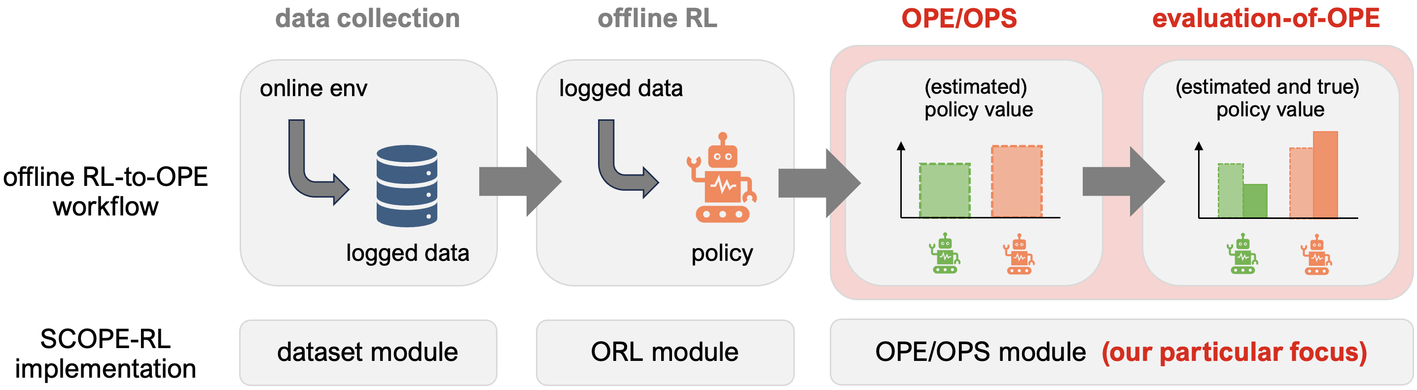
Figure 1: End-to-end workflow of offline RL and OPE with SCOPE-RL.

While existing packages offer flexible implementations for either offline RL or OPE, none currently provide a comprehensive, end-to-end solution that encompasses offline RL, OPE, and evaluation-of-OPE metrics. SCOPE-RL bridges this gap, seamlessly integrating the implementation of offline RL and OPE processes in an end-to-end manner for the first time. Specifically, to streamline the implementation process, our package comprises four key modules, with a particular focus on the latter two, as depicted in Figure 1:

The “Dataset” module is responsible for data collection and generation from RL environments. Thanks to its compatibility with OpenAI Gym/Gymnasium [1]-like environments, SCOPE-RL can be applied to a wide range of environmental settings. Furthermore, SCOPE-RL’s compatibility with d3rlpy [37], which includes various online and offline RL algorithms, allows users to assess the effectiveness of offline RL algorithms and OPE estimators across diverse data collection policies and experimental configurations.

The “ORL” module in SCOPE-RL offers a user-friendly wrapper for developing new policies using various offline RL algorithms. While d3rlpy [37] already features an accessible API, it is primarily geared towards employing offline RL algorithms individually. To enhance the efficiency of the entire offline RL and OPE process, our ORL module facilitates the management of multiple datasets and algorithms within a single unified class as explained in Appendix B.2 in greater detail.

The core of SCOPE-RL lies in the “OPE” and “OPS” modules. As elaborated in the following sections, we have incorporated a diverse array of OPE estimators in SCOPE-RL, ranging from basic options [11, 20, 30, 42] to advanced estimators that use marginal importance sampling [13, 24, 46, 54, 55], and those tailored for cumulative distribution OPE [2, 8, 9]. Additionally, we include various evaluation-of-OPE metrics. These key features in SCOPE-RL allow for a more nuanced understanding of policy performance and the effectiveness of OPE estimators, such as estimating a policy’s performance distribution (CD-OPE), and evaluating OPE outcomes in terms of the risk-return tradeoff in downstream policy selection tasks, as illustrated in Figure 2.

SCOPE-RL also introduces meta-classes for managing OPE/OPS experiments and abstract base classes for implementing new OPE estimators. These features enable researchers to rapidly integrate and test their own algorithms within the SCOPE-RL framework, and aid practitioners in comprehending the characteristics of various OPE methods through empirical evaluation.

3 Implemented OPE estimators and evaluation-of-OPE metrics

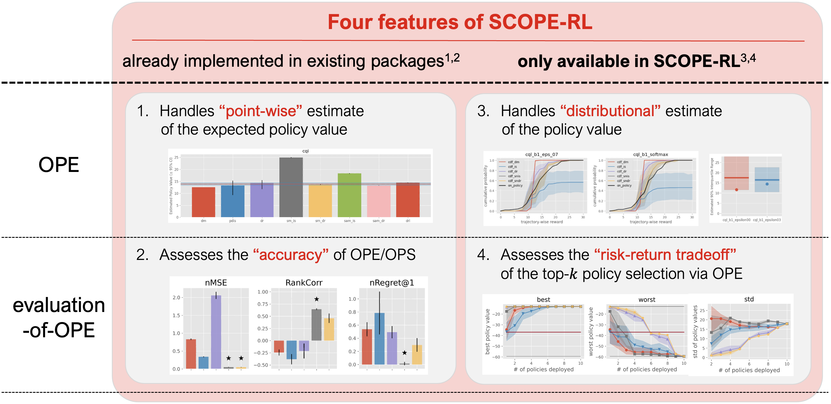
Figure 2: Summarizing the distinctive features of SCOPE-RL. OPE: While existing packages (e.g., [5, 49]) focus only on estimating the expected performance in a point-wise manner (left), SCOPE-RL additionally supports cumulative distribution OPE [2, 8, 9] to estimate the whole distribution of policy performance (right). Evaluation-of-OPE: While existing package reports only the “accuracy” of OPE or that of the downstream policy selection tasks [17] (left), SCOPE-RL also measures various risk-return tradeoff metrics in top-$k$ policy selection (right) (See Section 5 for the details). Visualization: Finally, all figures, including those illustrating the properties of existing packages, are generated by the visualization tools implemented in SCOPE-RL.

A distinctive contribution of SCOPE-RL is its comprehensive suite of OPE estimators. SCOPE-RL not only includes foundational OPE estimators like Fitted Q-Evaluation [20], Per-Decision Importance Sampling [30], and Doubly Robust [11, 42], but it also integrates advanced estimators that use state or state-action marginal importance weights [13, 24, 46, 55], high-confidence OPE [43, 44], and cumulative distribution OPE [2, 8, 9], alongside unique evaluation metrics for OPE [17].

In particular, the cumulative distribution OPE and the novel evaluation-of-OPE metrics set SCOPE-RL apart from existing OPE packages like [5, 20]. Through cumulative distribution OPE, SCOPE-RL is capable of estimating the entire performance distribution of a policy, in contrast to traditional OPE methods that only compute the point-wise expected policy performance [2, 8, 9]. Furthermore, our evaluation-of-OPE metrics, based on the statistics of the top-$k$ policies selected by OPE (“policy portfolio”), offer insights into the risk-return tradeoff in policy selection [17]. This approach transcends the conventional metrics such as Mean-Squared Error (MSE), Rank Correlation (RankCorr), and Regret, which focus only on “accuracy” in OPE and downstream policy selection. Consequently, SCOPE-RL enables a more multifaceted comparison of policy performance and the efficacy of OPE estimators compared to existing packages, as illustrated in Figure 2. We will delve into these key features of SCOPE-RL in greater detail in Sections 4 and 5.

The following is an overview of the OPE estimators and evaluation-of-OPE metrics implemented in SCOPE-RL. For a more comprehensive and rigorous understanding of each estimator’s definition and properties, please refer to Appendix A.

4 Key Feature 1: Cumulative distribution OPE

As introduced in Section 3, SCOPE-RL implements cumulative distribution OPE (CD-OPE) [2, 8, 9], which aims to estimate the full distribution of policy performance. To show the benefit of CD-OPE methods, we discuss the difference between (standard) OPE and CD-OPE in the following.

Preliminaries.

We consider a general RL setup, formalized by a Markov Decision Process (MDP) defined by the tuple $\langle\mathcal{S},\mathcal{A},\mathcal{T},P_{r},\gamma\rangle$. Here, $\mathcal{S}$ represents the state space and $\mathcal{A}$ denotes the action space, which can either be discrete or continuous. Let $\mathcal{T}:\mathcal{S}\times\mathcal{A}\rightarrow\mathcal{P}(\mathcal{S})$ be the state transition probability, where $\mathcal{T}(s^{\prime}|s,a)$ is the probability of observing state $s^{\prime}$ after taking action $a$ in state $s$. $P_{r}:\mathcal{S}\times\mathcal{A}\times\mathbb{R}\rightarrow[0,1]$ represents the probability distribution of the immediate reward, and $R(s,a):=\mathbb{E}_{r\sim P_{r}(r|s,a)}[r]$ is the expected immediate reward when taking action $a$ in state $s$. $\pi:\mathcal{S}\rightarrow\mathcal{P}(\mathcal{A})$ denotes a policy, where $\pi(a|s)$ is the probability of taking action $a$ in state $s$.

Off-Policy Evaluation (OPE).

In OPE, we are given a logged dataset collected by some behavior policy $\pi_{b}$ as follows.

$$\mathcal{D}:=\{(s_{t},a_{t},s_{t+1},r_{t})\}_{t=0}^{T-1}\sim p(s_{0})\prod_{t=0}^{T-1}\pi_{b}(a_{t}|s_{t})\mathcal{T}(s_{t+1}|s_{t},a_{t})P_{r}(r_{t}|s_{t},a_{t}).$$

Using only the fixed logged dataset $\mathcal{D}$, (standard) OPE aims to evaluate the expected reward under an evaluation (new) policy, called the policy value. More rigorously, the policy value is defined as the expected trajectory-wise reward obtained by deploying an evaluation policy $\pi$:

$$J(\pi):=\mathbb{E}_{\tau\sim p_{\pi}(\tau)}\left[\sum_{t=0}^{T-1}\gamma^{t}r_{t}\right],$$

where $\gamma\in(0,1]$ is a discount factor and $p_{\pi}(\tau)=p(s_{0})\prod_{t=0}^{T-1}\pi(a_{t}|s_{t})\mathcal{T}(s_{t+1}|s_{t},a_{t})P_{r}(r_{t}|s_{t},a_{t})$ is the probability of observing a trajectory under evaluation policy $\pi$.

While the typical definition of policy value effectively compares policies based on their expected performance, in practice, particularly in safety-critical scenarios, understanding the entire performance distribution of a policy is often more crucial and useful. For instance, in recommender systems, the aim is to consistently deliver good-quality recommendations rather than occasionally offering outstanding products while at other times significantly diminishing user satisfaction with poor choices. Similarly, in the context of self-driving cars, it is imperative to avoid catastrophic accidents, even if the probability of such events is extremely low (like less than 0.1%). In these situations, CD-OPE proves especially valuable for assessing the performance of policies in worst-case scenarios.

Cumulative Distribution Off-Policy Evaluation (CD-OPE).

In contrast to the traditional approach of OPE that focuses on the point-wise estimation of expected policy performance, CD-OPE seeks to estimate the entire performance distribution of a policy. Specifically, CD-OPE focuses on estimating the CDF of policy performance, providing a more comprehensive perspective on potential consequences [2, 8, 9]:

$$F(m,\pi):=\mathbb{E}\left[\mathbb{I}\left\{\sum_{t=0}^{T-1}\gamma^{t}r_{t}\leq m\right\}\mid\pi\right].$$

Based on the CDF ($F(\cdot)$), we can derive various risk functions on the policy performance as follows.

1. Mean: $\mu(F):=\int_{G}G\,\mathrm{d}F(G)$

2. Variance: $\sigma^{2}(F):=\int_{G}(G-\mu(F))^{2}\,\mathrm{d}F(G)$

3. $\alpha$-quartile: $Q^{\alpha}(F):=\min\{G\mid F(G)\leq\alpha\}$

4. Conditional Value at Risk (CVaR): $\int_{G}G\,\mathbb{I}\{G\leq Q^{\alpha}(F)\}\,\mathrm{d}F(G)$

where we define $G:=\sum_{t=0}^{T-1}\gamma^{t}r_{t}$ as the cumulative reward for a trajectory. The term $\mathrm{d}F(G):=\mathrm{lim}_{\Delta\rightarrow 0}F(G)-F(G-\Delta)$ represents the differential of the cumulative distribution function at $G$. The $\alpha$-quartile refers to the performance range extending from the lowest $100\times\alpha\,\%$ to the highest $100\times(1-\alpha)\,\%$ of observations. Conditional Value at Risk (CVaR) is calculated as the average of the lowest $100\times\alpha\,\%$ of these observations. These functions offer a more detailed analysis than just the expected performance, aiding practitioners in assessing the safety and robustness of a policy.

Figure 3 shows that SCOPE-RL enables implementing CD-OPE with minimal efforts.

⬇

# import modules and estimators for cumulative distribution OPE from SCOPE-RL

from scope_rl.ope import CumulativeDistributionOPE

from scope_rl.ope.discrete import CumulativeDistributionDM as CD_DM

from scope_rl.ope.discrete import CumulativeDistributionTIS as CD_IS

from scope_rl.ope.discrete import CumulativeDistributionTDR as CD_DR

from scope_rl.ope.discrete import CumulativeDistributionSNTIS as CD_SNIS

from scope_rl.ope.discrete import CumulativeDistributionSNTDR as CD_SNDR

# initialize CumulativeDistributionOPE class

cd_ope = CumulativeDistributionOPE(

logged_dataset=test_logged_dataset,

ope_estimators=[CD_DM(), CD_IS(), CD_DR(), CD_SNIS(), CD_SNDR()],

)

# estimate and visualize the cumulative distribution function

cdf_dict = cd_ope.estimate_cumulative_distribution_function(input_dict)

cd_ope.visualize_cumulative_distribution_function(input_dict)

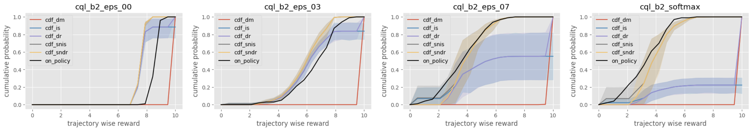
Figure 3: (Top) Example code of estimating the CDF with CD-OPE estimators implemented in SCOPE-RL. (Bottom) The output of the visualization function of the CD-OPE module.

5 Key Feature 2: Comprehensive evaluation-of-OPE metrics

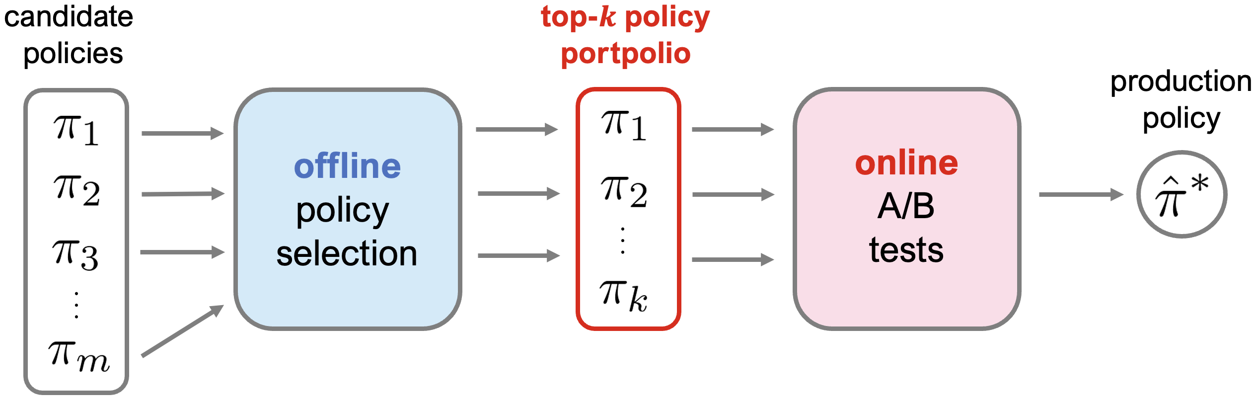
Figure 4: Practical workflow of policy evaluation and selection involves OPE as a screening process where an OPE estimator ($\hat{J}$) chooses top-$k$ (shortlisted) candidate policies that are to be tested in online A/B tests, where $k$ is a pre-defined online evaluation budget. A policy that is identified as the best policy based on the online evaluation process will be chosen as the production policy ($\hat{\pi}^{*}$). (Credit of the figure and description: [17])

Another distinctive feature of SCOPE-RL is to enable risk-return assessments of the downstream policy selection tasks (known as off-policy selection or OPS).

Background.

While OPE is a valuable tool for estimating the performance of new policies using offline logged data, it can sometimes yield inaccurate estimations due to bias and variance issues. Consequently, in real-world applications, it is imprudent to rely exclusively on OPE results for selecting a production policy. Instead, a combination of OPE results and online A/B testing is often employed for more comprehensive policy evaluation and selection [17, 19]. Typically, the practical workflow starts by using OPE results to eliminate underperforming policies. Subsequently, A/B tests are conducted on the remaining top-$k$ policies to determine the most effective one through a more dependable online evaluation, as depicted in Figure 4.

Evaluation of OPE.

To evaluate and compare the effectiveness of OPE estimators, the following accuracy metrics are often used:

• Mean Squared Error (MSE) [48, 49]: This metric measures the estimation accuracy of estimator $\hat{J}$ among a set of policies $\Pi$ as $(1/|\Pi|)\sum_{\pi\in\Pi}\mathbb{E}_{\mathcal{D}}[(\hat{J}(\pi;\mathcal{D})-J(\pi))^{2}]$.

• Rank Correlation (RankCorr) [5, 29]: This metric measures how well the ranking of candidate policies is preserved in the OPE results and is defined as the spearman’s rank correlation between $\{J(\pi)\}_{\pi\in\Pi}$ and $\{\hat{J}(\pi;\mathcal{D})\}_{\pi\in\Pi}$.

• Regret@$k$ [3]: This metric measures how well the best policy among the top-$k$ candidate policies selected by an estimator performs. In particular, Regret@1 measures the performance difference between the true best policy $\pi^{\ast}$ and the best policy estimated by the estimator as $J(\pi^{\ast})-J(\hat{\pi}^{\ast})$ where $\hat{\pi}^{\ast}:={\arg\max}_{\pi\in\Pi}\hat{J}(\pi;\mathcal{D})$.

In the aforementioned metrics, MSE evaluates the accuracy of OPE estimation, while the latter two metrics focus on the accuracy of downstream policy selection. By integrating these metrics, we can determine how effectively an OPE estimator selects a near-optimal policy based solely on OPE results. However, a significant limitation of this conventional approach for evaluation-of-OPE is that it fails to consider potential risks encountered during online A/B tests, especially in more practical two-stage selection processes that include online A/B testing as a final process [17].

To remedy this issue, SCOPE-RL offers evaluation-of-OPE metrics that evaluate the risk-return tradeoff in selecting the top-$k$ policies. Our fundamental approach involves treating the set of top-$k$ candidate policies chosen by an OPE estimator as its policy portfolio. Subsequently, we evaluate the risk, return, and efficiency of an estimator by reporting the following statistics of the top-$k$ policy portfolio:

• best@$\bm{k}$ (Return; higher is better): This metric represents the value of the highest-performing policy among the top-$k$ policies selected by an estimator. It indicates the effectiveness of the production policy chosen through top-$k$ A/B tests post-deployment.

• worst@$\bm{k}$, mean@$\bm{k}$ (Risk; higher is better): These metrics reveal the worst and average performance among the top-$k$ policies selected by an estimator. They provide insight into how well the policies tested in A/B tests perform on average and in the worst-case scenario.

• std@$\bm{k}$ (Risk; lower is better): This metric calculates the standard deviation of policy values among the top-$k$ policies chosen by an estimator. It indicates the likelihood of erroneously deploying poorly performing policies.

• safety violation rate@$\bm{k}$ (Risk; lower is better): This metric quantifies the probability of policies deployed in online A/B tests violating predefined safety requirements.

• SharpeRatio@k (Efficiency; higher is better): This metric evaluates the return (best@$k$) relative to a risk-free baseline ($J(\pi_{b})$), considering the risk (std@$k$) in its denominator. This provides a measure of efficiency balancing risk and return.

  $$\text{SharpeRatio@}k(\hat{J}):=\frac{\text{best@}k(\hat{J})-J(\pi_{b})}{\text{std@}k(\hat{J})}.$$

  By comparing the SharpeRatio metric, we can identify an OPE estimator that is capable of deploying policies which not only enhance performance over the baseline but also minimize risks. Note that this metric is the main proposal of our sister paper [17].

Using the SCOPE-RL package, we can also evaluate how the risk-return tradeoff metrics change with varying online evaluation budgets ($k$) in online A/B tests (See examples in Figure 5).

⬇

from scope_rl.ope import OffPolicySelection

# initialize the OPS class with OPE instances

ops = OffPolicySelection(

ope=ope,

cumulative_distribution_ope=cd_ope,

)

# visualize the top k deployment result

ops.visualize_topk_policy_value_selected_by_standard_ope(

input_dict=input_dict,

compared_estimators=["dm", "tis", "pdis", "dr"],

metrics=["best", "worst", "std", "sharpe_ratio"],

relative_safety_criteria=1.0,

)

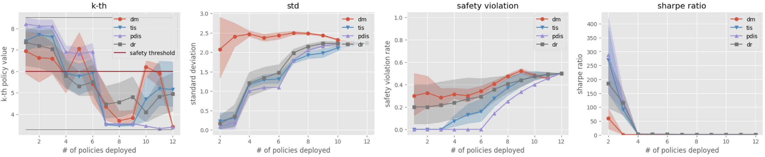
Figure 5: (Top) Example code to perform evaluation-of-OPE with SharpRatio@k and other statistics of top-$k$ policy portfolio using SCOPE-RL. (Bottom) Visualizing the evaluation-of-OPE results.

6 User-friendly APIs, visualization tools, and documentation

SCOPE-RL’s user-friendly APIs and comprehensive support for implementation are among its key attributes. As demonstrated in Figures 3 and 5 and further detailed in Appendix B, SCOPE-RL allows for the management of the entire offline RL-to-OPE process with just a few lines of code. Additionally, visualizing results is straightforward and offers valuable insights for comparing various policies and OPE estimators.

Customizing modules in SCOPE-RL is also streamlined, thanks to our comprehensive support resources. These include API references, detailed usage guides, and quickstart examples, all designed to provide clear instructions for various implementation options. This enables users to effortlessly test their own OPE estimators in different environmental settings or with real-world datasets. We believe SCOPE-RL greatly facilitates rapid benchmarking and practical application of offline RL and OPE in both research and practice.

7 Summary and Future Work

This paper introduces SCOPE-RL, a Python package tailored for offline RL and OPE, with a special emphasis on OPE modules. SCOPE-RL pioneers the implementation of cutting-edge cumulative distribution OPE (CD-OPE) and evaluation-of-OPE metrics through risk-return tradeoffs. Additionally, our extensive, well-structured documentation and intuitive APIs aid researchers and practitioners in efficiently implementing offline RL and OPE procedures.

For future developments, we aim to enhance SCOPE-RL further. Potential updates include integrating more advanced CD-OPE estimators [9, 51, 53], estimators for partially observable settings [47], and estimator selection methods for OPE [21, 39, 45, 52, 58]. Adding tutorials on OPE to our documentation could also be valuable, helping users grasp OPE concepts more clearly. We also welcome and encourage pull requests, suggestions, and feedback from the user community.

Lastly, SCOPE-RL draws inspiration from OpenBanditPipeline [34], which has been successful in facilitating flexible OPE experiments in contextual bandits [26, 45, 33, 36] and slate bandits [16, 18]. We believe that SCOPE-RL will similarly become a valuable tool for quick prototyping and benchmarking in the OPE of RL policies, paralleling OBP’s role in non-RL contexts.

Appendix A Details of implemented OPE estimators and assessment metrics

Here, we provide the definition and properties of OPE estimators and assessment metrics implemented in SCOPE-RL, which are listed in Section 3.

A.1 Standard Off-Policy Evaluation

As described in the main text, the goal of OPE in RL is to estimate the expected trajectory-wise reward under an evaluation policy $\pi$ using only the logged data $\mathcal{D}$ collected by a behavior policy $\pi_{b}$:

$$J(\pi):=\mathbb{E}_{\tau\sim p_{\pi}(\tau)}\left[\sum_{t=0}^{T-1}\gamma^{t}r_{t}\right].$$

Direct Method (DM)

DM is a model-based approach, which uses the initial state value estimated by Fitted Q Evaluation (FQE) [20]. It first learns the Q-function from the logged data via temporal-difference (TD) learning and then utilizes the estimated Q-function for OPE as follows.

$$\hat{J}_{\mathrm{DM}}(\pi;\mathcal{D}):=\frac{1}{n}\sum_{i=1}^{n}\sum_{a\in\mathcal{A}}\pi(a|s_{0}^{(i)})\hat{Q}(s_{0}^{(i)},a)=\frac{1}{n}\sum_{i=1}^{n}\hat{V}(s_{0}^{(i)}),$$

where $\hat{Q}(s_{t},a_{t})$ is an estimated state-action value and $\hat{V}(s_{t})$ is the estimated state value. DM has lower variance compared to other estimators, but can produce large bias caused by approximation errors of the Q-function [11, 42].

Trajectory-wise Importance Sampling (TIS)

TIS is a model-free approach, which uses the importance sampling technique to correct the distribution shift between $\pi$ and $\pi_{b}$ as follows [30].

$$\hat{J}_{\mathrm{TIS}}(\pi;\mathcal{D}):=\frac{1}{n}\sum_{i=1}^{n}\sum_{t=0}^{T-1}\gamma^{t}w_{1:T-1}^{(i)}r_{t}^{(i)},$$

where $w_{0:T-1}:=\prod_{t=0}^{T-1}(\pi(a_{t}|s_{t})/\pi_{b}(a_{t}|s_{t}))$ is the (trajectory-wise) importance weight. TIS enables unbiased estimation of the policy value. However, particularly when the trajectory length $T$ and the action space $\mathcal{A}$ is large, TIS suffers from high variance due to trajectory-wise importance weighting [11, 42].

Per-Decision Importance Sampling (PDIS)

PDIS leverages the sequential nature of the MDP to reduce the variance of TIS. Specifically, since $s_{t}$ only depends on the states and actions observed previously (i.e., $s_{0},\ldots,s_{t-1}$ and $a_{0},\ldots,a_{t-1}$) and is independent of those observed in future time steps (i.e., $s_{t+1},\ldots,s_{T}$ and $a_{t+1},\ldots,a_{T}$), PDIS considers only the importance weights related to past interactions for each time step as follows [30].

$$\hat{J}_{\mathrm{PDIS}}(\pi;\mathcal{D}):=\frac{1}{n}\sum_{i=1}^{n}\sum_{t=0}^{T-1}\gamma^{t}w_{0:t}^{(i)}r_{t}^{(i)},$$

where $w_{0:t}:=\prod_{t^{\prime}=0}^{t}(\pi(a_{t^{\prime}}\mid s_{t^{\prime}})/\pi_{b}(a_{t^{\prime}}\mid s_{t^{\prime}}))$ represents the importance weight with respect to the previous action choices for time step $t$. PDIS retains its unbiased nature while reducing the variance of TIS. However, it is well-known that PDIS can still suffer from high variance when $T$ is large [11, 42].

Doubly Robust (DR)

DR is a hybrid of model-based estimation and importance sampling [4]. It introduces $\hat{Q}$ as a baseline estimation in the recursive form of PDIS and applies importance weighting only to its residual [11, 42].

$$\hat{J}_{\mathrm{DR}}(\pi;\mathcal{D}):=\frac{1}{n}\sum_{i=1}^{n}\sum_{t=0}^{T-1}\gamma^{t}\left(w_{0:t}^{(i)}(r_{t}^{(i)}-\hat{Q}(s_{t}^{(i)},a_{t}^{(i)}))+w_{0:t-1}^{(i)}\sum_{a\in\mathcal{A}}\pi(a|s_{t}^{(i)})\hat{Q}(s_{t}^{(i)},a)\right),$$

As $\hat{Q}$ works as a control variate, DR is unbiased and at the same time reduces the variance of TIS when $\hat{Q}(\cdot)$ is reasonably accurate. However, it can still have high variance when the trajectory length $T$ [5] or the action space $|\mathcal{A}|$ [33] is large.

Self-Normalized estimators

Self-normalized estimators aim to reduce the scale of the importance weight for the variance reduction purpose [40]. Specifically, the self-normalized versions of PDIS and DR are defined as follows.

$$\hat{J}_{\mathrm{SNPDIS}}(\pi;\mathcal{D}):=\sum_{i=1}^{n}\sum_{t=0}^{T-1}\gamma^{t}\frac{w_{0:t}^{(i)}}{\sum_{i^{\prime}=1}^{n}w_{0:t}^{(i^{\prime})}}r_{t}^{(i)},$$

$$\hat{J}_{\mathrm{SNDR}}(\pi;\mathcal{D})$$

$$:=\sum_{i=1}^{n}\sum_{t=0}^{T-1}\gamma^{t}\left(\frac{w_{0:t}^{(i)}}{\sum_{i^{\prime}=1}^{n}w_{0:t}^{(i^{\prime})}}(r_{t}^{(i)}-\hat{Q}(s_{t}^{(i)},a_{t}^{(i)}))+\frac{w_{0:t-1}^{(i)}}{\sum_{i^{\prime}=1}^{n}w_{0:t-1}^{(i^{\prime})}}\sum_{a\in\mathcal{A}}\pi(a|s_{t}^{(i)})\hat{Q}(s_{t}^{(i)},a)\right),$$

In more general, self-normalized estimators substitute importance weight $w_{\ast}$ as $\tilde{w}_{\ast}:=w_{\ast}/(\sum_{i=1}^{n}w_{\ast})$, where $\tilde{w}_{\ast}$ is called the self-normalized importance weight. While self-normalized estimators no longer ensures unbiasedness, they basically remain consistent. Moreover, self-normalized estimators have the variance bounded by $r_{max}^{2}$, which is much smaller than the variance of the original estimators [12].

Marginalized Importance Sampling estimators

When the trajectory length ($T$) is large, the variance of PDIS and DR can be very high. This issue is often referred to as the curse of horizon in OPE. To alleviate this variance issue of the estimators that rely on importance weights with respect to the policies, several estimators utilize state marginal or state-action marginal importance weights, which are defined as follows [24, 46]:

$$\rho(s,a):=d^{\pi}(s,a)/d^{\pi_{b}}(s,a),\quad\quad\quad\quad\quad\rho(s):=d^{\pi}(s)/d^{\pi_{b}}(s)$$

where $d^{\pi}(s,a)$ and $d^{\pi}(s)$ is the marginal visitation probability of the policy $\pi$ on $(s,a)$ or $s$, respectively. The use of marginal importance weights is particularly beneficial when policy visits the same or similar states among different trajectories or different timestep. (e.g., when the state transition is something like $\cdots\rightarrow s_{1}\rightarrow s_{2}\rightarrow s_{1}\rightarrow s_{2}\rightarrow\cdots$ or when the trajectories always visit some particular state as $\cdots\rightarrow s_{*}\rightarrow s_{1}\rightarrow s_{*}\rightarrow\cdots$). Then, State-Action Marginal Importance Sampling (SMIS) and State Marginal Doubly Robust (SMDR) are defined as follows.

$$\hat{J}_{\mathrm{SAM-IS}}(\pi;\mathcal{D}):=\frac{1}{n}\sum_{i=1}^{n}\sum_{t=0}^{T-1}\gamma^{t}\rho(s_{t}^{(i)},a_{t}^{(i)})r_{t}^{(i)},$$

$$\hat{J}_{\mathrm{SAM-DR}}(\pi;\mathcal{D})$$

$$:=\frac{1}{n}\sum_{i=1}^{n}\sum_{a\in\mathcal{A}}\pi(a|s_{0}^{(i)})\hat{Q}(s_{0}^{(i)},a)$$

$$\quad\quad+\frac{1}{n}\sum_{i=1}^{n}\sum_{t=0}^{T-1}\gamma^{t}\rho(s_{t}^{(i)},a_{t}^{(i)})\left(r_{t}^{(i)}+\gamma\sum_{a\in\mathcal{A}}\pi(a|s_{t}^{(i)})\hat{Q}(s_{t+1}^{(i)},a)-\hat{Q}(s_{t}^{(i)},a_{t}^{(i)})\right),$$

Similarly, State-Marginal Importance Sampling (SMIS) and State Action-Marginal Doubly Robust (SAMDR) are defined as follows.

$$\hat{J}_{\mathrm{SM-IS}}(\pi;\mathcal{D}):=\frac{1}{n}\sum_{i=1}^{n}\sum_{t=0}^{T-1}\gamma^{t}\rho(s_{t}^{(i)})w_{t}(s_{t}^{(i)},a_{t}^{(i)})r_{t}^{(i)},$$

$$\hat{J}_{\mathrm{SM-DR}}(\pi;\mathcal{D})$$

$$:=\frac{1}{n}\sum_{i=1}^{n}\sum_{a\in\mathcal{A}}\pi(a|s_{0}^{(i)})\hat{Q}(s_{0}^{(i)},a)$$

$$\quad\quad+\frac{1}{n}\sum_{i=1}^{n}\sum_{t=0}^{T-1}\gamma^{t}\rho(s_{t}^{(i)})w_{t}(s_{t}^{(i)},a_{t}^{(i)})\left(r_{t}^{(i)}+\gamma\sum_{a\in\mathcal{A}}\pi(a|s_{t}^{(i)})\hat{Q}(s_{t+1}^{(i)},a)-\hat{Q}(s_{t}^{(i)},a_{t}^{(i)})\right),$$

Table 2: Correspondence between the hyperparameter setups of Augmented Lagrangian Method (ALM) [54] and other weight learning methods.

hyperparameters	$\alpha_{w}\in[0,\infty)$	$\alpha_{Q}\in[0,\infty)$	$\alpha_{r}\in\{0,1\}$	$\lambda\in(-\infty,\infty)$
BestDICE [54]	1	0	1	(optimize)
DualDICE [27]	0	1	0	0
GenDICE [56]	0	1	0	(optimize)
GradientDICE [57]	0	1	0	(optimize)
AlgaeDICE [28]	1	0	1	0
MQL/MWL [46]	0	0	0	0

Note: $\alpha_{w}$ and $\alpha_{Q}$ are hyperparameters that regularize the complexity of the weight and value functions. $\alpha_{r}$ is the scaling factor of the reward. $\lambda$ is the normalization constraint that enforces $\mathbb{E}_{\mathcal{D}_{\pi_{b}}}[w(s,a)]$ to be 1. For the theoretical analysis, we refer readers to [54].

How to obtain state(-action) marginal importance weight?  To utilize marginalized importance sampling estimators, we first need to estimate the state marginal or state-action marginal importance weight. A prevalent method for this involves leveraging the relationship between the importance weights and the state-action value function, under the assumption that the state visitation probability remains consistent across various timesteps [46].

$$\mathbb{E}_{(s,a,r,s^{\prime})\sim\mathcal{D}_{\pi_{b}}}[w(s,a)r]$$

$$=\mathbb{E}_{(s,a,r,s^{\prime})\sim\mathcal{D}_{\pi_{b}}}[w(s,a)(Q_{\pi}(s,a)-\gamma\mathbb{E}_{a^{\prime}\sim\pi(a^{\prime}|s^{\prime})}[Q(s^{\prime},a^{\prime})])]$$

$$=(1-\gamma)\mathbb{E}_{s_{0}\sim d^{\pi}(s_{0}),a_{0}\sim\pi(a_{0}|s_{0})}[Q_{\pi}(s_{0},a_{0})]$$

Weight learning aims to minimize the discrepancy between the middle term and the last term of the equation provided above. This is achieved when the Q-function adversarially maximizes the difference. In particular, we use the following algorithms to estimate state marginal and state-action marginal importance weights (and the corresponding state-action value function).

• Augmented Lagrangian Method (ALM/DICE) [54]:
  This method simultaneously optimize both $w(s,a)$ and $Q(s,a)$ via the following objective.

  $$\max_{w\leq 0}\min_{Q,\lambda}L(w,Q,\lambda),$$

  $$L(w,Q,\lambda)$$

  $$:=(1-\gamma)\mathbb{E}_{s_{0}\sim d(s_{0}),a_{0}\sim\pi(s_{0})}[Q(s_{0},a_{0})]+\lambda$$

  $$\quad+\mathbb{E}_{\tau_{t}\sim d^{\pi_{b}},a_{t+1}\sim\pi(a_{t+1}|s_{t+1})}[w(s_{t},a_{t})(\alpha_{r}r_{t}+\gamma Q(s_{t+1},a_{t+1})-Q(s_{t},a_{t})-\lambda)]$$

  $$\quad+\alpha_{Q}\mathbb{E}_{(s_{t},a_{t})\sim d^{\pi_{b}}}[Q^{2}(s_{t},a_{t})]-\alpha_{w}\mathbb{E}_{(s_{t},a_{t})\sim d^{\pi_{b}}}[w^{2}(s_{t},a_{t})]$$

  where $\tau_{t}:=(s_{t},a_{t},r_{t},s_{t+1})$ is a data tuple in the logged data. $\alpha_{w}\in[0,\infty)$, $\alpha_{Q}\in[0,\infty)$, $\alpha_{r}\in\{0,1\}$, $\lambda\in(-\infty,\infty)$ are the regularization hyperparameters. By setting different hyperparameters, ALM is reduced to BestDICE [54], DualDICE [27], GenDICE [56], GradientDICE [57], AlgaeDICE [28], and MQL/MWL [46]. We describe the correspondence between hyperparameter setup of ALM and other algorithms in Table 2.

• Minimax Q-Learning and Weight Learning (MQL/MWL) [46]:
  This method operates under the assumption that either the value function or the weight function is expressed by a function class within a reproducing kernel Hilbert space (RKHS). It optimizes solely either the value function or the weight function.
  
  In particular, when learning a weight function, MWL optimizes the function approximation using the following objective:

  $$\max_{w}L_{w}^{2}(w,Q),$$

  $$L_{w}^{2}(w,Q) =\mathbb{E}_{\tau_{t},\tilde{\tau}_{t}\sim d^{\pi_{b}},a_{t+1}\sim\pi(a_{t+1}|s_{t+1}),\tilde{a}_{t+1}\sim\pi(\tilde{a}_{t+1}|\tilde{s}_{t+1})}[$$

  $$\quad\quad\quad w(s_{t},a_{t})w(\tilde{s}_{t},\tilde{a}_{t})(K((s_{t},a_{t}),(\tilde{s}_{t},\tilde{a}_{t}))+K((s_{t+1},a_{t+1}),(\tilde{s}_{t+1},\tilde{a}_{t+1}))$$

  $$\quad\quad\quad-\gamma(K((s_{t},a_{t}),(\tilde{s}_{t+1},\tilde{a}_{t+1}))+K((s_{t+1},a_{t+1}),(\tilde{s}_{t},\tilde{a}_{t}))))]$$

  $$\quad\quad+\gamma(1-\gamma)\mathbb{E}_{\tau_{t},\tilde{\tau}_{t}\sim d^{\pi_{b}},a_{t+1}\sim\pi(a_{t+1}|s_{t+1}),\tilde{a}_{t+1}\sim\pi(\tilde{a}_{t+1}|\tilde{s}_{t+1}),(s_{0},a_{0}),(\tilde{s}_{0},\tilde{a}_{0})\sim d^{\pi}_{0}}[$$

  $$\quad\quad\quad w(s_{t},a_{t})K((s_{t+1},a_{t+1}),(\tilde{s}_{0},\tilde{a}_{0}))+w(\tilde{s}_{t},\tilde{a}_{t})K((\tilde{s}_{t+1},\tilde{a}_{t+1}),(s_{0},a_{0}))]$$

  $$\quad\quad-(1-\gamma)\mathbb{E}_{(s_{t},a_{t}),(\tilde{s}_{t},\tilde{a}_{t})\sim d^{\pi_{b}},s_{0}\sim d(s_{0}),\tilde{s}_{0}\sim d(\tilde{s}_{0}),a_{0}\sim\pi(a_{0}|s_{0}),\tilde{a}_{0}\sim\pi(\tilde{a}_{0}|\tilde{s}_{0})}[$$

  $$\quad\quad\quad w(s_{t},a_{t})K((s_{t},a_{t}),(\tilde{s}_{0},\tilde{a}_{0}))+w(\tilde{s}_{t},\tilde{a}_{t})K((\tilde{s}_{t},\tilde{a}_{t}),(s_{0},a_{0}))]$$

  where $\tau_{t}:=(s_{t},a_{t},r_{t},s_{t+1})$ is a data tuple and $K(\cdot,\cdot)$ is a kernel function. $(\tilde{s}_{0},\tilde{a}_{0})\sim d^{\pi}_{0}$ indicates that the initial state is sampled as $s_{0}\sim d(s_{0})$ and the initial action is sampled as $a_{0}\sim\pi(a_{0}|s_{0})$.
  
  In contrast, when learning a Q-function, MQL learns from the following objective.

  $$\max_{Q}L_{Q}^{2}(w,Q),$$

  $$L_{Q}^{2}(w,Q) =\mathbb{E}_{\tau_{t},\tilde{\tau}_{t}\sim d^{\pi_{b}},a_{t+1}\sim\pi(a_{t+1}|s_{t+1}),\tilde{a}_{t+1}\sim\pi(\tilde{a}_{t+1}|\tilde{s}_{t+1})}[$$

  $$\quad\quad\quad(r_{t}+\gamma Q(s_{t+1},a_{t+1})-Q(s_{t},a_{t}))$$

  $$\quad\quad\quad\cdot K((s_{t},a_{t}),(\tilde{s}_{t},\tilde{a}_{t}))(\tilde{r}_{t}+\gamma Q(\tilde{s}_{t+1},\tilde{a}_{t+1})-Q(\tilde{s}_{t},\tilde{a}_{t}))]$$

  where $\tau_{t}:=(s_{t},a_{t},r_{t},s_{t+1})$ is a data tuple and $K(\cdot,\cdot)$ is a kernel function.

Double Reinforcement Learning (DRL)

DRL [13] leverages marginal importance sampling in the definition of DR as follows.

$$\hat{J}_{\mathrm{DRL}}(\pi;\mathcal{D})$$

$$:=\frac{1}{n}\sum_{k=1}^{K}\sum_{i=1}^{n_{k}}\sum_{t=0}^{T-1}(\rho^{j}(s_{t}^{(i)},a_{t}^{(i)})(r_{t}^{(i)}-Q^{j}(s_{t}^{(i)},a_{t}^{(i)}))+\rho^{j}(s_{t-1}^{(i)},a_{t-1}^{(i)})\sum_{a\in\mathcal{A}}\pi(a|s_{t}^{(i)})Q^{j}(s_{t}^{(i)},a)).$$

DRL achieves the semiparametric efficiency bound with a consistent value estimator $\hat{Q}$. To alleviate the potential bias introduced in $\hat{Q}$, DRL employs the cross-fitting technique to estimate the value function. Specifically, let $K$ represent the number of folds and $\mathcal{D}_{j}$ denote the $j$-th split of logged data, consisting of $n_{k}$ samples. The cross-fitting procedure obtains $\hat{w}^{j}$ and $\hat{Q}^{j}$ on the subset of data used for OPE, that is, $\mathcal{D}\setminus\mathcal{D}_{j}$.

Spectrum of Off-Policy Estimators (SOPE)

While the state marginal or state-action marginal importance weights effectively alleviate the variance issue of per-decision importance weighting, particularly when the trajectory is long, the estimation error of marginal importance weights may introduce some bias in the estimation. To alleviate this and control the bias-variance tradeoff more flexibly, SOPE uses the following interpolated importance weights [55].

$$w_{\mathrm{SOPE}}(s_{t},a_{t}) =\begin{cases}\prod_{t^{\prime}=0}^{k-1}w_{t}(s_{t^{\prime}},a_{t^{\prime}})&\mathrm{if}\,t<k\\ \rho(s_{t-k},a_{t-k})\prod_{t^{\prime}=t-k+1}^{t}w_{t}(s_{t^{\prime}},a_{t^{\prime}})&\mathrm{otherwise}\end{cases}$$

$$w_{\mathrm{SOPE}}(s_{t},a_{t}) =\begin{cases}\prod_{t^{\prime}=0}^{k-1}w_{t}(s_{t^{\prime}},a_{t^{\prime}})&\mathrm{if}\,t<k\\ \rho(s_{t-k})\prod_{t^{\prime}=t-k}^{t}w_{t}(s_{t^{\prime}},a_{t^{\prime}})&\mathrm{otherwise}\end{cases}$$

where SOPE uses the per-decision importance weight $w_{t}(s_{t},a_{t}):=\pi(a_{t}|s_{t})/\pi_{b}(a_{t}|s_{t})$ for the $k$ most recent timesteps.

For instance, State Action-Marginal Importance Sampling (SAMIS) and State Action-Marginal Doubly Robust (SAM-DR) are defined as follows.

$$\hat{J}_{\mathrm{SOPE-SAM-IS}}(\pi;\mathcal{D}):=\frac{1}{n}\sum_{i=1}^{n}\sum_{t=0}^{k-1}\gamma^{t}w_{0:t}^{(i)}r_{t}^{(i)}+\frac{1}{n}\sum_{i=1}^{n}\sum_{t=k}^{T-1}\gamma^{t}\rho(s_{t-k}^{(i)},a_{t-k}^{(i)})w_{t-k+1:t}^{(i)}r_{t}^{(i)},$$

$$\hat{J}_{\mathrm{SOPE-SAM-DR}}(\pi;\mathcal{D})$$

$$:=\frac{1}{n}\sum_{i=1}^{n}\sum_{a\in\mathcal{A}}\pi(a|s_{0}^{(i)})\hat{Q}(s_{0}^{(i)},a)$$

$$\quad\quad+\frac{1}{n}\sum_{i=1}^{n}\sum_{t=0}^{k-1}\gamma^{t}w_{0:t}^{(i)}\left(r_{t}^{(i)}+\gamma\sum_{a\in\mathcal{A}}\pi(a|s_{t}^{(i)})\hat{Q}(s_{t+1}^{(i)},a)-\hat{Q}(s_{t}^{(i)},a_{t}^{(i)})\right)$$

$$\quad\quad+\frac{1}{n}\sum_{i=1}^{n}\sum_{t=k}^{T-1}\gamma^{t}\rho(s_{t-k}^{(i)},a_{t-k}^{(i)})w_{t-k+1:t}^{(i)}\left(r_{t}^{(i)}+\gamma\sum_{a\in\mathcal{A}}\pi(a|s_{t}^{(i)})\hat{Q}(s_{t+1}^{(i)},a)-\hat{Q}(s_{t}^{(i)},a_{t}^{(i)})\right),$$

High Confidence Off-Policy Evaluation

To mitigate the risk of overestimating the policy value due to high variance, we sometimes aim to estimate both the confidence interval and an appropriate lower bound of the policy value. SCOPE-RL implements four methods to estimate these confidence intervals [43, 44].

1. Hoeffding: $\,|\hat{J}(\pi;\mathcal{D})-\mathbb{E}_{\mathcal{D}}[\hat{J}(\pi;\mathcal{D})]|\leq\hat{J}_{\max}\displaystyle\sqrt{\frac{\log(1/\alpha)}{2n}}$

2. Empirical Bernstein: $\,|\hat{J}(\pi;\mathcal{D})-\mathbb{E}_{\mathcal{D}}[\hat{J}(\pi;\mathcal{D})]|\leq\displaystyle\frac{7\hat{J}_{\max}\log(2/\alpha)}{3(n-1)}+\displaystyle\sqrt{\frac{2\hat{\mathbb{V}}_{\mathcal{D}}(\hat{J})\log(2/\alpha)}{(n-1)}}$

3. Student T-test: $\,|\hat{J}(\pi;\mathcal{D})-\mathbb{E}_{\mathcal{D}}[\hat{J}(\pi;\mathcal{D})]|\leq\displaystyle\frac{T_{\mathrm{test}}(1-\alpha,n-1)}{\sqrt{n}/\hat{\sigma}}$

4. Bootstrapping: $\,|\hat{J}(\pi;\mathcal{D})-\mathbb{E}_{\mathcal{D}}[\hat{J}(\pi;\mathcal{D})]|\leq\mathrm{Bootstrap}(1-\alpha)$

All the above bounds hold with a probability of $1-\alpha$. In terms of notation, we denote $\hat{\mathbb{V}}_{\mathcal{D}}(\cdot)$ as the sample variance, $T_{\mathrm{test}}(\cdot,\cdot)$ as the T-value, and $\sigma$ as the standard deviation. Among the above high confidence interval estimations, the Hoeffding and empirical Bernstein methods derive lower bounds without imposing any distribution assumption on the reward, which sometimes results in overly conservative estimations. On the other hand, the T-test is based on the assumption that each sample follows a normal distribution. Thus, when the true distribution of an estimator is highly skewed, the lower bound based T-test may not hold, but it can derive a tighter bound compared to those of the Hoeffding and empirical Bernstein methods when the assumption holds.

Extension to the continuous action space

When the action space is continuous, the naive importance weight $w_{t}=\pi(a_{t}|s_{t})/\pi_{b}(a_{t}|s_{t})=\int_{a\in\mathcal{A}}(\pi(a|s_{t})/\pi_{b}(a_{t}|s_{t}))\mathbb{I}(a=a_{t})da$ ends up rejecting almost all actions, as $\mathbb{I}(a=a_{t})$ filters only the action observed in the logged data. To address this issue, continuous OPE estimators apply the kernel density estimation technique to smooth the importance weight as follows [14].

$$\overline{w}_{t}=\int_{a\in\mathcal{A}}\frac{\pi(a|s_{t})}{\pi_{b}(a_{t}|s_{t})}\cdot\frac{1}{h}K\left(\frac{a-a_{t}}{h}\right)da,$$

where $K(\cdot)$ denotes a kernel function and $h$ is the bandwidth hyperparameter. A large value of $h$ leads to a high-bias but low-variance estimator, while a small value of $h$ results in a low-bias but high-variance estimator. Any function that can be represented as $K(\cdot)$ and satisfies the following regularity conditions can be used as the kernel function:

1. $\int xK(x)dx=0$

2. $\int K(x)dx=1$

3. $\lim_{x\rightarrow-\infty}K(x)=\lim_{x\rightarrow+\infty}K(x)=0$

4. $K(x)\geq 0,\forall x$

We provide the following kernel functions in SCOPE-RL.

• Gaussian kernel: $K(x)=\frac{1}{\sqrt{2\pi}}e^{-\frac{x^{2}}{2}}$

• Epanechnikov kernel: $K(x)=\frac{3}{4}(1-x^{2})\,(|x|\leq 1)$

• Triangular kernel: $K(x)=1-|x|\,(|x|\leq 1)$

• Cosine kernel: $K(x)=\frac{\pi}{4}\mathrm{cos}\left(\frac{\pi}{2}x\right)\,(|x|\leq 1)$

• Uniform kernel: $K(x)=\frac{1}{2}\,(|x|\leq 1)$

A.2 Cumulative Distribution Off-Policy Evaluation

In practical situations, we often have a greater interest in risk functions such as Conditional Value at Risk (CVaR) and the interquartile range of the trajectory-wise reward under an evaluation policy, rather than the mere expectation (i.e., policy value). To derive these risk functions, Cumulative Distribution Off-Policy Evaluation (CD-OPE) first estimates the following cumulative distribution function (CDF) [2, 8, 9].

$$F(m,\pi):=\mathbb{E}\left[\mathbb{I}\left\{\sum_{t=0}^{T-1}\gamma^{t}r_{t}\leq m\right\}\mid\pi\right],$$

which allows us to derive various risk functions based on $F(\cdot)$ as follows.

1. Mean: $\mu(F):=\int_{G}G\,\mathrm{d}F(G)$

2. Variance: $\sigma^{2}(F):=\int_{G}(G-\mu(F))^{2}\,\mathrm{d}F(G)$

3. $\alpha$-quartile: $Q^{\alpha}(F):=\min\{G\mid F(G)\leq\alpha\}$

4. Conditional Value at Risk (CVaR): $\int_{G}G\,\mathbb{I}\{G\leq Q^{\alpha}(F)\}\,\mathrm{d}F(G)$

where we let $G:=\sum_{t=0}^{T-1}\gamma^{t}r_{t}$ to denote the trajectory wise reward and $\mathrm{d}F(G):=\mathrm{lim}_{\Delta\rightarrow 0}F(G)-F(G-\Delta)$. $\alpha$-quartile is the performance range from $100\times\alpha\,\%$ to $100\times(1-\alpha)\,\%$. CVaR is the average among the lower $100\times\alpha\,\%$ of the observations. These functions provide more fine-grained information about the policy performance than the expected trajectory-wise reward.

Below, we describe estimators for estimating the CDF ($F(m,\pi)$) supported by SCOPE-RL.

Direct Method (DM)

DM adopts a model-based approach to estimate the cumulative distribution function (CDF) [8].

$$\hat{F}_{\mathrm{DM}}(m,\pi;\mathcal{D}):=\frac{1}{n}\sum_{i=1}^{n}\sum_{a\in\mathcal{A}}\pi(a|s_{0}^{(i)})\hat{G}(m;s_{0}^{(i)},a)$$

where $\hat{F}(\cdot)$ is the estimated CDF and $\hat{G}(\cdot)$ is an estimator for $\mathbb{E}\left[\sum_{t=0}^{T-1}\gamma^{t}r_{t}\mid s,a\right]$. DM is vulnerable to the approximation error and resulting bias issue, but has lower variance than other estimators, similar to the basic OPE.

Trajectory-wise Importance Sampling (TIS)

TIS corrects the distribution shift by applying the importance sampling technique on the CDF estimation [2, 8].

$$\hat{F}_{\mathrm{TIS}}(m,\pi;\mathcal{D}):=\frac{1}{n}\sum_{i=1}^{n}w_{0:T-1}^{(i)}\mathbb{I}\left\{\sum_{t=0}^{T-1}\gamma^{t}r_{t}^{(i)}\leq m\right\}$$

TIS is unbiased but can suffer from high variance. As a consequence, $\hat{F}_{\mathrm{TIS}}(\cdot)$ sometimes becomes more than 1.0 when the variance is high. Therefore, we correct CDF as follows [8].

$$\hat{F}^{\ast}_{\mathrm{TIS}}(m,\pi;\mathcal{D}):=\min(\max_{m^{\prime}\leq m}\hat{F}_{\mathrm{TIS}}(m^{\prime},\pi;\mathcal{D}),1).$$

Trajectory-wise Doubly Robust (TDR)

TDR combines TIS and DM as follows [8].

$$\hat{F}_{\mathrm{TDR}}(m,\pi;\mathcal{D}):=\frac{1}{n}\sum_{i=1}^{n}w_{0:T-1}^{(i)}\left(\mathbb{I}\left\{\sum_{t=0}^{T-1}\gamma^{t}r_{t}^{(i)}\leq m\right\}-\hat{G}(m;s_{0}^{(i)},a_{0}^{(i)})\right)+\hat{F}_{\mathrm{DM}}(m,\pi;\mathcal{D})$$

TDR reduces the variance of TIS while being unbiased, leveraging the model-based estimate (i.e., DM) as a control variate. Since $\hat{F}_{\mathrm{TDR}}(\cdot)$ may take a value outsize the required rage of [0, 1], we should apply the following transformation to bound $\hat{F}_{\mathrm{TDR}}(\cdot)\in[0,1]$ [8].

$$\hat{F}^{\ast}_{\mathrm{TDR}}(m,\pi;\mathcal{D}):=\mathrm{clip}(\max_{m^{\prime}\leq m}\hat{F}_{\mathrm{TDR}}(m^{\prime},\pi;\mathcal{D}),0,1).$$

Note that this estimator is not equivalent to the (recursive) DR estimator defined by [9]. We plan to implement the recursive version in future updates of the software.

Self-Normalized estimators

We also provide self-normalized estimators for the CDF, which normalize the importance weight as $\tilde{w}_{\ast}:=w_{\ast}/\sum_{i=1}^{n}w{\ast}$ for variance reduction. Using the self-normalized importance weights, $\hat{F}_{\mathrm{SNTIS}}(\cdot)$ never exceeds one. On the other hand, $\hat{F}_{\mathrm{SNTDR}}(\cdot)$ still requires clipping to keep $\hat{F}_{\mathrm{SNTDR}}(\cdot)$ within the range of $[0,1]$.

Plans for additional implementations

Cumulative Distribution Off-Policy Evaluation (CD-OPE) is garnering increasing attention and has become an active area of research. While we currently provide the baseline estimators proposed by [2, 8], we aim to continue adding advanced CD-OPE estimators in future updates. For instance, the addition of a recursive DR estimator proposed by [9] would be beneficial for reducing variance caused by the trajectory-wise importance weights. Additionally, the inclusion of generative modeling-based OPE estimators [51, 53] will enable more flexible control of the bias-variance tradeoff via the bandwidth parameter of the kernel function.

A.3 Evaluation metrics for OPE and OPS

SCOPE-RL provides both conventional evaluation protocols and risk-return tradeoff metrics to evaluate OPE and OPS methods. First, we implement the following four metrics to measure the accuracy of OPE estimators, the first three of which are the baseline conventional metrics described in the main text:

• Mean Squared Error (MSE) [49]: This metric measures the estimation accuracy of estimator $\hat{J}$ across a set of policies $\Pi$ as follows:

  $$\mathrm{MSE}(\hat{J}):=\frac{1}{|\Pi|}\sum_{\pi\in\Pi}\mathbb{E}_{\mathcal{D}}[(\hat{J}(\pi;\mathcal{D})-J(\pi))^{2}].$$

• Rank Correlation (Rankcorr) [5, 29]: This metric measures how well the ranking of the candidate policies is preserved in the OPE results. It is defined as the (expected) Spearman’s rank correlation between $\{J(\pi)\}_{\pi\in\Pi}$ and $\{\hat{J}\{\pi;\mathcal{D})\}_{\pi\in\Pi}$ as

  $$\mathrm{RankCorr}(\hat{J}):=\frac{\mathrm{cov}(R_{J}(\Pi),R_{\hat{J}}(\Pi))}{\mathrm{std}(R_{J}(\Pi))\,\mathrm{std}(R_{\hat{J}}(\Pi))}=1-\frac{6\sum_{\pi\in\Pi}(R_{J}(\pi)-R_{\hat{J}}(\pi))^{2}}{k(k^{2}-1)},$$

  where $R_{J}(\cdot)$ is the ranking of candidate policy based on $J(\cdot)$, while $R_{\hat{J}}(\cdot)$ is the ranking estimated by an OPE estimator $\hat{J}$. $\mathrm{cov}(R_{J}(\Pi),R_{\hat{J}}(\Pi))$ is the covariance between the two rankings, and $\mathrm{std}(R_{\cdot}(\Pi))$ is the standard deviation of the ranking indexes, which is constant across all possible rankings.

• Regret@$\bm{k}$ [3]: This metric measures how well the best policy among the top-$k$ candidate policies selected by an estimator performs. It is defined as follows:

  $$\text{Regret@}k(\hat{J}):=\max_{\pi\in\Pi}J(\pi)-\max_{\pi\in\Pi_{k}(\hat{J})}J(\pi).$$

  In particular, Regret@1 measures the performance difference between the true best policy $\pi^{\ast}$ and the best policy estimated by an estimator as $J(\pi^{\ast})-J(\hat{\pi}^{\ast})$, where $\hat{\pi}^{\ast}:={\arg\max}_{\pi\in\Pi}\hat{J}(\pi;\mathcal{D})$.

• Type I and Type II Error Rates: These metrics measure how well an OPE estimator validates whether the policy performance surpasses the given safety threshold or not. Below are the definitions of the Type I and Type II error rates:

  $$\text{Type I error rate }(\hat{J}) :=\frac{\sum_{\pi\in\Pi}\mathbb{I}\,\{\hat{J}(\pi)\geq\bar{J}\}\cap\mathbb{I}\,\{J(\pi)<\bar{J}\}}{\sum_{\pi\in\Pi}\mathbb{I}\,\{J(\pi)<\bar{J}\}},$$

  $$\text{Type II error rate }(\hat{J}) :=\frac{\sum_{\pi\in\Pi}\mathbb{I}\,\{\hat{J}(\pi)<\bar{J}\}\cap\mathbb{I}\,\{J(\pi)\geq\bar{J}\}}{\sum_{\pi\in\Pi}\mathbb{I}\,\{J(\pi)\geq\bar{J}\}},$$

  where $\mathbb{I}\,\{\cdot\}$ is the indicator function and $\bar{J}$ is a safety threshold.

In addition to the above metrics, we measure the top-$k$ deployment performance to evaluate the outcome of policy selection:

• best@$\bm{k}$ (return; the larger, the better): This metric reports the best policy performance among the selected top-$k$ policies as

  $$\text{best@}k(\hat{J}):=\max_{\pi\in\Pi_{k}(\hat{J})}J(\pi).$$

  Similar to regret@$k$, this metric measures how well an OPE estimator identifies a high-performing policy.

• worst@$\bm{k}$, mean@$\bm{k}$ (risk; the larger, the better): These metrics report the worst and mean performance among the top-$k$ policies selected by an estimator as

  $$\text{worst@}k(\hat{J}):=\min_{\pi\in\Pi_{k}(\hat{J})}J(\pi),\quad\quad\text{mean@}k(\hat{J}):=\frac{1}{|\Pi_{k}(\hat{J})|}\sum_{\pi\in\Pi_{k}(\hat{J})}J(\pi).$$

  These metrics quantify how likely an OPE estimator mistakenly chooses poorly-performing policies as promising.

• std@$\bm{k}$ (risk; the smaller, the better): This metric reports how the performance among top-$k$ policies deviates from each other as

  $$\text{std@}k(\hat{J}): =\sqrt{\frac{1}{k}\sum_{\pi\in\Pi_{k}(\hat{J})}\left(J(\pi)-\left(\frac{1}{k}\sum_{\pi\in\Pi_{k}(\hat{J})}J(\pi)\right)\right)^{2}}.$$

  This metric also quantifies how likely an OPE estimator is to mistakenly chooses poorly-performing policies.

• safety violation rate@$\bm{k}$ (risk; the smaller, the better): This metric reports the probability of deployed policies violating a pre-defined safety requirement $\bar{J}$ (such as the performance of the behavior policy) as follows.

  $$\text{safety violation rate@}k(\hat{J}): =\frac{1}{|\Pi_{k}(\hat{J})|}\sum_{\pi\in\Pi_{k}(\hat{J})}\mathbb{I}\,\{J(\pi)<\bar{J}\}.$$

• Sharpe ratio@$\bm{k}$ (efficiency; the larger, the better): Analogous to the original Sharpe ratio used in the field of finance [38], we define this metric as

  $$\text{SharpeRatio@}k(\hat{J}):=\frac{\text{best@}k(\hat{J})-J(\pi_{b})}{\text{std@}k(\hat{J})}.$$

  This metric measures the return (best@$k$) over the risk-free baseline ($J(\pi_{b})$) while accounting for risk (std@$k$) in the denominator [17].

These metrics can be seen as the statistics of the policy portfolio formed by a given OPE estimator. Note that these metrics are also applicable not only to standard OPE but also to cumulative distribution OPE (e.g., our implementation can measure the top-$k$ performance metric of CVaR instead of the policy value $J(\pi)$).

Appendix B Example codes and tutorials of SCOPE-RL

Here, we provide some example end-to-end codes to implement offline RL, OPE, and assessments of OPE and OPS via SCOPE-RL. For more detailed usages, please also refer to https://scope-rl.readthedocs.io/en/latest/documentation/examples/index.html.

B.1 Handling a single logged dataset

We first show the case of using a single logged dataset generated by a single behavior policy. Note that we use a sub-package of SCOPE-RL called “BasicGym” as a simple and synthetic RL environment in the following examples.

⬇

# setting up basicgym

import gym

import basicgym

env = gym.make("BasicEnv-discrete-v0")

Code Snippet 1: Setting up an synthetic environment

B.1.1 Synthetic Data Generation

To perform an end-to-end process of offline RL and OPE, we need a logged dataset generated by a behavior policy. Thus, we first train a base behavior policy using d3rlpy [37] as follows.

⬇

# behavior policy

from d3rlpy.algos import DoubleDQNConfig

from d3rlpy.models.encoders import VectorEncoderFactory

from d3rlpy.models.q_functions import MeanQFunctionFactory

from d3rlpy.dataset import create_fifo_replay_buffer

from d3rlpy.algos import LinearDecayEpsilonGreedy

# model

ddqn = DoubleDQNConfig(

encoder_factory=VectorEncoderFactory(hidden_units=[30, 30]),

q_func_factory=MeanQFunctionFactory(),

).create()

# replay buffer

buffer = create_fifo_replay_buffer(

limit=10000,

env=env,

)

# explorers

explorer = LinearDecayEpsilonGreedy(

start_epsilon=1.0,

end_epsilon=0.1,

duration=1000,

)

# online training

ddqn.fit_online(

env,

buffer,

explorer=explorer,

eval_env=env,

n_steps=100000,

)

Code Snippet 2: Training a base behavior policy

After obtaining a base behavior policy, we make it stochastic and generate logged datasets based on it. The two independent logged datasets correspond are used for performing offline RL and OPE, respectively.

⬇

# import SCOPE-RL modules

from scope_rl.dataset import SyntheticDataset

from scope_rl.policy import EpsilonGreedyHead

# converting the behavior policy to a stochastic one

behavior_policy = EpsilonGreedyHead(

ddqn,

n_actions=env.action_space.n,

epsilon=0.3,

name="ddqn_epsilon_0.3",

random_state=12345,

)

# initialize the dataset class

dataset = SyntheticDataset(

env=env,

max_episode_steps=env.step_per_episode,

)

# generate logged data for offline RL

train_logged_dataset = dataset.obtain_episodes(

behavior_policies=behavior_policy,

n_trajectories=10000,

random_state=12345,

)

# generate logged data for OPE

test_logged_dataset = dataset.obtain_episodes(

behavior_policies=behavior_policy,

n_trajectories=10000,

random_state=12345 + 1,

)

Code Snippet 3: Generating a synthetic logged dataset

B.1.2 Offline Reinforcement Learning

Next, we train new (and hopefully better) policies from only offline logged data. Since we use d3rlpy [37] for this offline RL part, we first transform the logged dataset to a d3rlpy format. As shown below, SCOPE-RL provides a smooth integration with d3rlpy.

⬇

# import d3rlpy modules

from d3rlpy.dataset import MDPDataset

# transform offline dataset to a d3rlpy format

offlinerl_dataset = MDPDataset(

observations=train_logged_dataset["state"],

actions=train_logged_dataset["action"],

rewards=train_logged_dataset["reward"],

terminals=train_logged_dataset["done"],

)

Code Snippet 4: Dataset compatibility with d3rlpy

Then, we train several offline RL algorithms as follows.

⬇

from d3rlpy.algos import DiscreteCQLConfig as CQLConfig

# prepare models

cql_b1 = CQLConfig(

encoder_factory=VectorEncoderFactory(hidden_units=[30, 30]),

q_func_factory=MeanQFunctionFactory(),

).create()

cql_b2 = CQLConfig(

encoder_factory=VectorEncoderFactory(hidden_units=[100]),

q_func_factory=MeanQFunctionFactory(),

).create()

cql_b3 = CQLConfig(

encoder_factory=VectorEncoderFactory(hidden_units=[50, 10]),

q_func_factory=MeanQFunctionFactory(),

).create()

algos = [cql_b1, cql_b2, cql_b3]

# learn base evaluation policies

for i in range(len(algos)):

algos[i].fit(

offlinerl_dataset,

n_steps=10000,

)

# make stochastic candidate policies

evaluation_policies = []

for i in range(len(algos)):

for j, epsilon in enumerate([0.3, 0.5, 0.7]):

eval_policy = EpsilonGreedyHead(

base_policy=algos[i],

n_actions=env.action_space.n,

name=f"cql_b{i+1}_epsilon_{epsilon}",

epsilon=epsilon,

random_state=12345,

)

evaluation_policies.append(eval_policy)

Code Snippet 5: Offline Reinforcement Learning

B.1.3 Off-Policy Evaluation

After deriving several candidate policies, we go on to evaluate their performance (policy value) using the logged data via OPE. Here, we use the following OPE estimators implemented in SCOPE-RL.

⬇

# basic estimators

from scope_rl.ope.discrete import DirectMethod as DM

from scope_rl.ope.discrete import SelfNormalizedPDIS as SNPDIS

from scope_rl.ope.discrete import SelfNormalizedDR as SNDR

# marginal importance sampling-based estimators

from scope_rl.ope.discrete import StateMarginalSNIS as SMSNIS

from scope_rl.ope.discrete import StateMarginalSNDR as SMSNDR

from scope_rl.ope.discrete import StateActionMarginalSNIS as SAMSNIS

from scope_rl.ope.discrete import StateActionMarginalSNDR as SAMSNDR

from scope_rl.ope.discrete import DoubleReinforcementLearning as DRL

# initializing OPE estimators

ope_estimators = [

DM(), SNPDIS(), SNDR(), SMSNIS(), SMSNDR(), SAMSNIS(), SAMSNDR(), DRL(),

]

Code Snippet 6: Representative OPE estimators implemented in SCOPE-RL

Even with some advanced OPE estimators, such as marginal importance sampling-based estimators, SCOPE-RL enables OPE process in an easily implementable way as follows.

⬇

# import ope modules from SCOPE-RL

from scope_rl.ope import CreateOPEInput

from scope_rl.ope import OffPolicyEvaluation as BasicOPE

# create inputs for OPE

prep = CreateOPEInput(env)

input_dict = prep.obtain_whole_inputs(

logged_dataset=test_logged_dataset,

evaluation_policies=evaluation_policies,

require_value_prediction=True,

require_weight_prediction=True, # to estimate marginal importance weights

n_trajectories_on_policy_evaluation=100,

random_state=12345,

)

# conduct OPE and visualize the result

ope = BasicOPE(

logged_dataset=test_logged_dataset,

ope_estimators=ope_estimators,

)

policy_value_df, policy_value_interval_df = ope.summarize_off_policy_estimates(

input_dict=input_dict,

random_state=12345,

)

ope.visualize_off_policy_estimates(

input_dict,

hue="policy",

sharey=False,

random_state=12345,

)

Code Snippet 7: Basic Off-Policy Evaluation

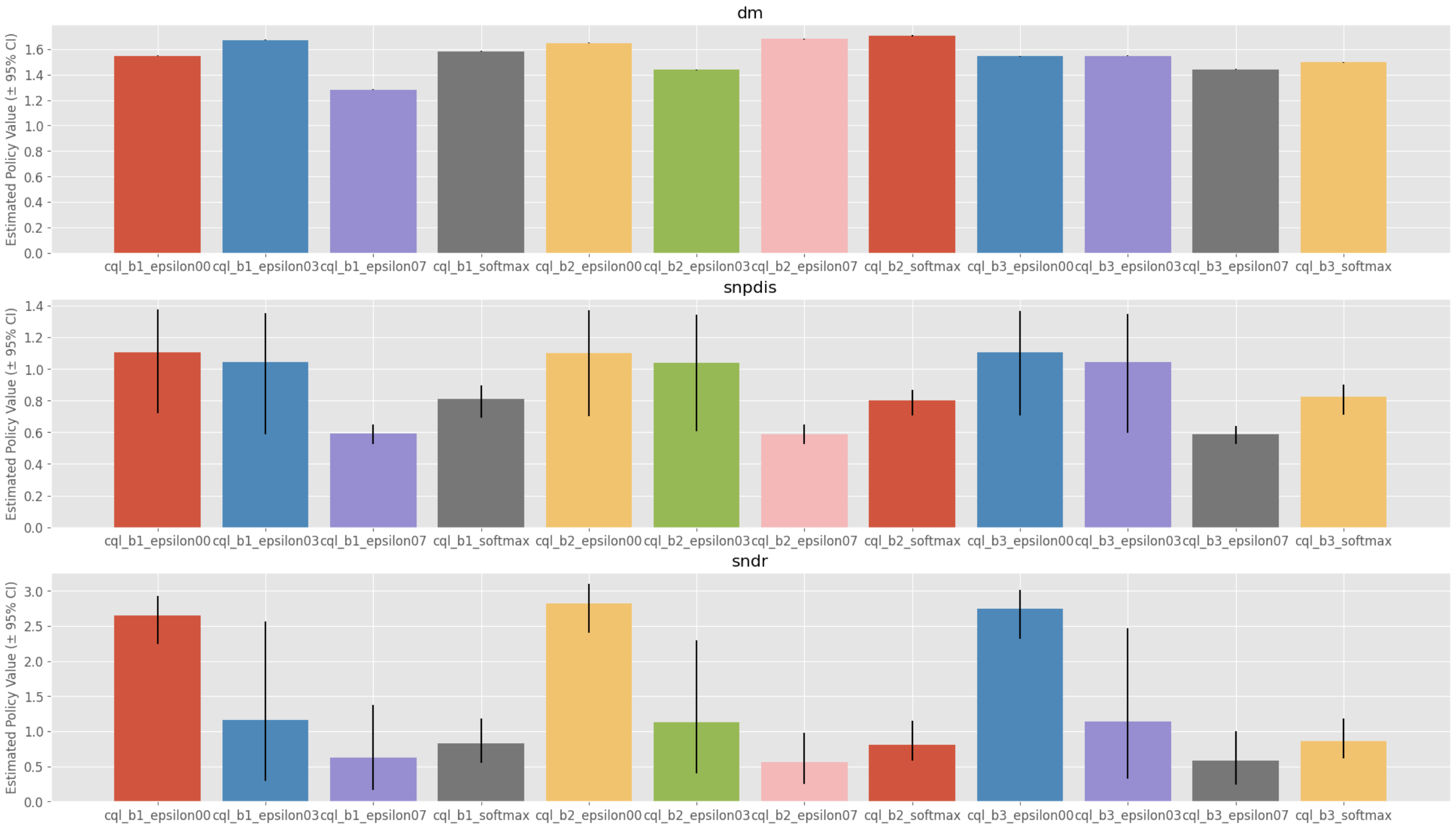
Figure 6: Example of estimating policy value with basic OPE estimators.

We can also perform CD-OPE in a manner similar to basic OPE as follows.

⬇

# import modules and estimators for cumulative distribution OPE from SCOPE-RL

from scope_rl.ope import CumulativeDistributionOPE

from scope_rl.ope.discrete import CumulativeDistributionDM as CD_DM

from scope_rl.ope.discrete import CumulativeDistributionTIS as CD_IS

from scope_rl.ope.discrete import CumulativeDistributionTDR as CD_DR

from scope_rl.ope.discrete import CumulativeDistributionSNTIS as CD_SNIS

from scope_rl.ope.discrete import CumulativeDistributionSNTDR as CD_SNDR

# initialize CumulativeDistributionOPE class

cd_ope = CumulativeDistributionOPE(

logged_dataset=test_logged_dataset,

ope_estimators=[CD_DM(), CD_IS(), CD_DR(), CD_SNIS(), CD_SNDR()],

)

# estimate and visualize the cumulative distribution function

cdf_dict = cd_ope.estimate_cumulative_distribution_function(input_dict)

cd_ope.visualize_cumulative_distribution_function(input_dict, n_cols=4)

Code Snippet 8: Cumulative Distribution Off-Policy Evaluation

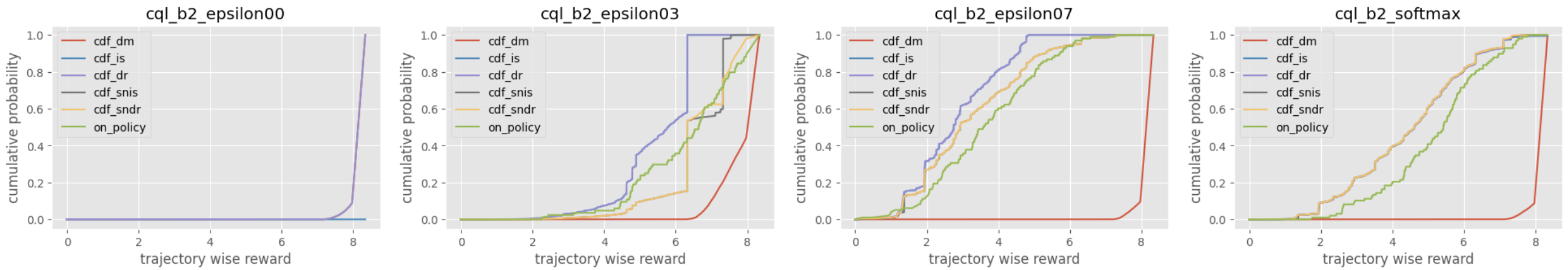
Figure 7: Example of estimating Cumulative Distribution Function (CDF) with CD-OPE estimators.

Similarly, SCOPE-RL is also able to visualize the Conditional Value ar Risk (CVaR) and the interquartile range of the trajectory-wise reward under the evaluation policy as follows.

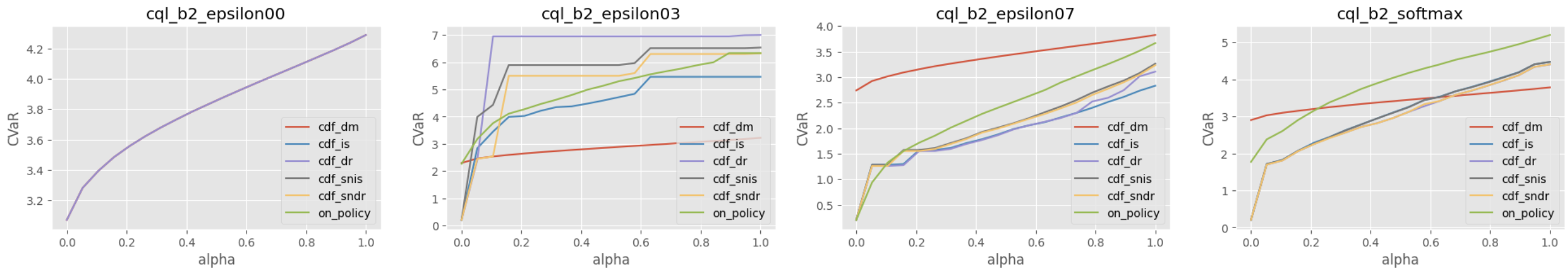
Figure 8: Example of estimating the Conditional Value at Risk (CVaR) with CD-OPE estimators.

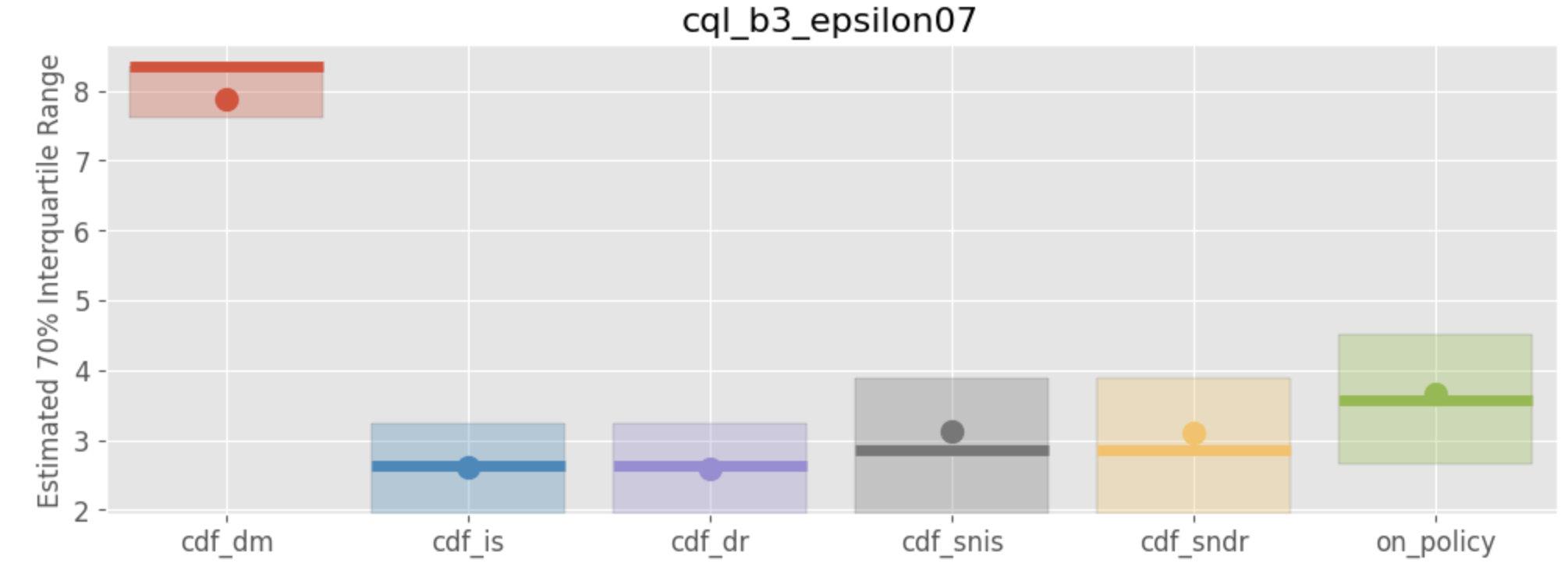
Figure 9: Example of estimating the interquartile range with CD-OPE estimators.

B.1.4 Off-Policy Selection and Assessments of OPE

Finally, we conduct OPS based on OPE results. We can also evaluate the performance of OPE estimators with SharpRatio@k and other statistics of top-$k$ policies selected by each OPE estimator.

⬇

# import the OPS module from SCOPE-RL

from scope_rl.ope import OffPolicySelection

# initialize the OPS class with OPE instances

ops = OffPolicySelection(

ope=ope,

cumulative_distribution_ope=cd_ope,

)

# rank candidate policy by estimated lower quartile and evaluate the OPE results

ranking_df, metric_df = ops.select_by_lower_quartile(

input_dict,

alpha=0.3,

return_metrics=True,

return_by_dataframe=True,

)

# visualize the top k deployment result

ops.visualize_topk_policy_value_selected_by_standard_ope(

input_dict=input_dict,

compared_estimators=["dm", "snpdis", "sndr", "drl"],

metrics=["best", "worst", "std", "sharpe_ratio"],

relative_safety_criteria=1.0,

)

# compare the true and estimated policy performances

ops.visualize_policy_value_for_validation(

input_dict=input_dict,

compared_estimators=["dm", "snpdis", "sndr", "drl"],

)

Code Snippet 9: Off-Policy Selection and Assessments of OPE

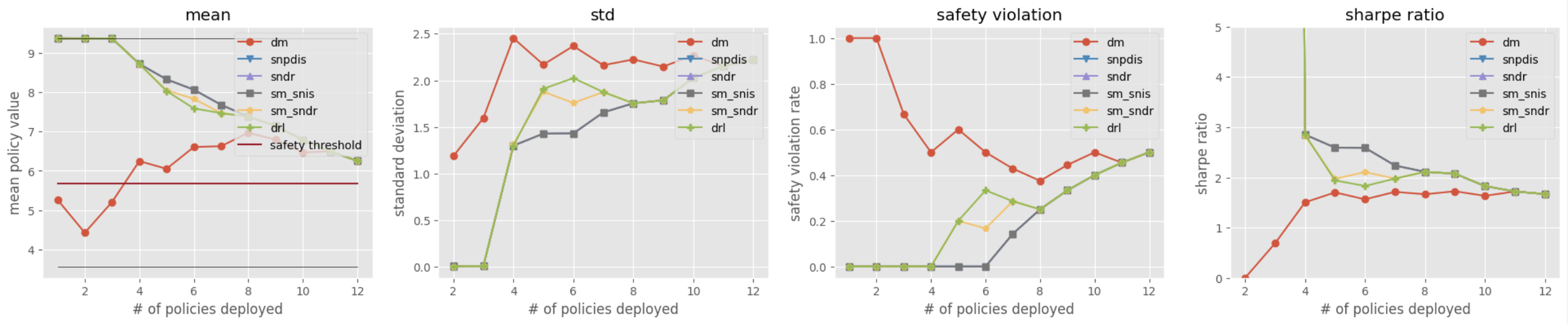
Figure 10: Example of assessing OPE with SharpRatio@k and other statistics of top-$k$ policy portfolio.

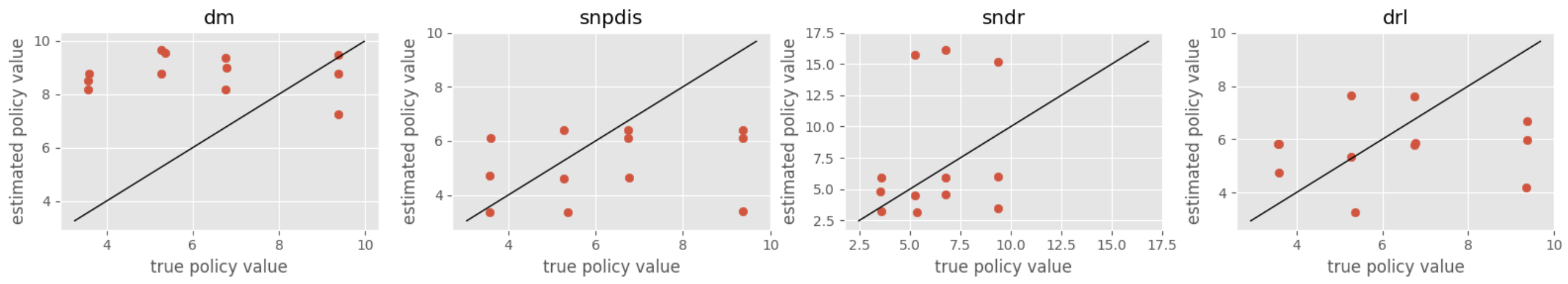
Figure 11: Example of comparing the true and estimated policy value for validation.

B.2 Handling multiple logged datasets

SCOPE-RL enables us to conduct OPE and the whole offline RL procedure on multiple logged dataset without additional effort. Below, we show how to handle multiple logged datasets generated by multiple different behavior policies.

B.2.1 Synthetic Data Generation

We generate logged datasets with several behavior policies that have different levels of exploration.

⬇

from scope_rl.dataset import SyntheticDataset

from scope_rl.policy import EpsilonGreedyHead

# define behavior policies

behavior_policies = []

for i, epsilon in enumerate([0.1, 0.3, 0.5]):

behavior_policy = EpsilonGreedyHead(

ddqn,

n_actions=env.action_space.n,

epsilon=epsilon,

name=f"ddqn_eps_{epsilon}",

random_state=12345,

)

behavior_policies.append(behavior_policy)

# initialize dataset class

dataset = SyntheticDataset(

env=env,

max_episode_steps=env.step_per_episode,

)

# generate logged datasets by multiple behavior policies

train_logged_dataset = dataset.obtain_episodes(

behavior_policies=behavior_policies, #

n_datasets=10, # number of logged datasets for each behavior policy

n_trajectories=10000,

random_state=12345,

)

test_logged_dataset = dataset.obtain_episodes(

behavior_policies=behavior_policies, #

n_datasets=10, # number of logged datasets for each behavior policy

n_trajectories=10000,

random_state=12345 + 1,

)

Code Snippet 10: Generating logged datasets with multiple behavior policies

B.2.2 Offline Reinforcement Learning

To ease the offline policy learning process with multiple logged datasets, SCOPE-RL provides an easy-to-use wrapper for Offline learning. Below, we show the example of obtaining candidate policies with 3 base policies and 2 parameters for exploration as follows.

⬇

# base algorithms

cql_b1 = CQLConfig(

encoder_factory=VectorEncoderFactory(hidden_units=[30, 30]),

q_func_factory=MeanQFunctionFactory(),

).create()

cql_b2 = CQLConfig(

encoder_factory=VectorEncoderFactory(hidden_units=[100]),

q_func_factory=MeanQFunctionFactory(),

).create()

cql_b3 = CQLConfig(

encoder_factory=VectorEncoderFactory(hidden_units=[50, 10]),

q_func_factory=MeanQFunctionFactory(),

).create()

algorithms = [cql_b1, cql_b2, cql_b3]

algorithms_name = ["cql_b1", "cql_b2", "cql_b3"]

# exploration hyperparameters

policy_wrappers = {

"eps_03": (

EpsilonGreedyHead, {

"epsilon": 0.3,

"n_actions": env.action_space.n,

}

),

"eps_05": (

EpsilonGreedyHead, {

"epsilon": 0.7,

"n_actions": env.action_space.n,

}

),

}

Code Snippet 11: Base algorithms and exploration hyperparameters of candidate policies

The OPL class trains candidate policies with given algorithms on multiple logged datasets.

⬇

# import the OPL module from SCOPE-RL

from scope_rl.policy import TrainCandidatePolicies

# initialize the OPL class

orl = TrainCandidatePolicies()

# obtain base policies

base_policies = orl.learn_base_policy(

logged_dataset=train_logged_dataset,

algorithms=algorithms,

random_state=12345,

)

# define evaluation policies

eval_policies = orl.apply_head(

base_policies=base_policies,

base_policies_name=algorithms_name,

policy_wrappers=policy_wrappers,

random_state=12345,

)

Code Snippet 12: Offline Reinforcement Learning (with multiple logged dataset)

B.2.3 Off-Policy Evaluation

SCOPE-RL is also capable of handling OPE with multiple logged datasets in a manner similar to that of a single logged dataset as follows.

⬇

from scope_rl.ope import OffPolicyEvaluation as BasicOPE

from scope_rl.ope import CreateOPEInput

# OPE estimators

from scope_rl.ope.discrete import DirectMethod as DM

from scope_rl.ope.discrete import TrajectoryWiseImportanceSampling as TIS

from scope_rl.ope.discrete import PerDecisionImportanceSampling as PDIS

from scope_rl.ope.discrete import DoublyRobust as DR

from scope_rl.ope.discrete import SelfNormalizedTIS as SNTIS

from scope_rl.ope.discrete import SelfNormalizedPDIS as SNPDIS

from scope_rl.ope.discrete import SelfNormalizedDR as SNDR

# prepare OPE inputs

prep = CreateOPEInput(

env=env,

)

input_dict = prep.obtain_whole_inputs(

logged_dataset=test_logged_dataset, #

evaluation_policies=eval_policies,

require_value_prediction=True,

n_trajectories_on_policy_evaluation=100,

)

# initialize the OPE class with multiple logged datasets

ope = BasicOPE(

logged_dataset=test_logged_dataset, #

ope_estimators=[DM(), TIS(), PDIS(), DR(), SNTIS(), SNPDIS(), SNDR()],

)

# note: the results for each dataset are accessible via ‘‘policy_value_df_dict[behavior_policy.name][dataset_id]‘‘

policy_value_df_dict, policy_value_interval_df_dict = ope.summarize_off_policy_estimates(

input_dict=input_dict,

random_state=12345,

)

# conduct OPE with multiple logged datasets and visualize the result

ope.visualize_policy_value_with_multiple_estimates(

input_dict,

hue="policy",

)

Code Snippet 13: Basic Off-Policy Evaluation (with multiple logged datasets)

Figure 12: Example of comparing estimated policy value across multiple logged datasets.

Similarly, SCOPE-RL can handle CD-OPE with multiple logged datasets quite easily.

⬇

from scope_rl.ope import CumulativeDistributionOPE

from scope_rl.ope.discrete import CumulativeDistributionDM as CD_DM

from scope_rl.ope.discrete import CumulativeDistributionTIS as CD_IS

from scope_rl.ope.discrete import CumulativeDistributionTDR as CD_DR

from scope_rl.ope.discrete import CumulativeDistributionSNTIS as CD_SNIS

from scope_rl.ope.discrete import CumulativeDistributionSNTDR as CD_SNDR

# initialize the CD-OPE class with multiple logged datasets

cd_ope = CumulativeDistributionOPE(

logged_dataset=test_logged_dataset, #

ope_estimators=[CD_DM(), CD_IS(), CD_DR(), CD_SNIS(), CD_SNDR()],

)

# note: the results for each dataset are accessible via ‘‘policy_value_dict[behavior_policy.name][dataset_id]‘‘

policy_value_dict = cd_ope.estimate_mean(input_dict)

# estimate and visualize CDF with multiple logged datasets

cd_ope.visualize_cumulative_distribution_function_with_multiple_estimates(

input_dict,

behavior_policy_name=behavior_policies[0].name, # specify behavior policy name

plot_type="ci_hue", #

scale_min=0.0, # set reward scale (i.e., x-axis or bins of CDF)

scale_max=10.0,

n_partition=20,

n_cols=4,

)

Code Snippet 14: Cumulative Distribution Off-Policy Evaluation (with multiple logged datasets)

Figure 13: Example of estimating Conditional Value at Risk (CVaR) with CD-OPE estimators on multiple logged datasets.

B.2.4 Off-Policy Selection and Assessments of OPE

Finally, we can also conduct OPS and assess the OPE results with multiple logged datasets as follows.

⬇

from scope_rl.ope import OffPolicySelection

# initialize the OPS class with OPE instances

ops = OffPolicySelection(

ope=ope,

cumulative_distribution_ope=cd_ope,

)

# note: the results for each dataset are accessible via ‘‘ranking_df_dict[behavior_policy.name][dataset_id]‘‘ and ‘‘metric_df_dict[behavior_policy.name][dataset_id]‘‘

ranking_df_dict, metric_df_dict = ops.select_by_lower_quartile(

input_dict,

alpha=0.3,

return_metrics=True,

return_by_dataframe=True,

)

# visualize the top k deployment result

ops.visualize_topk_policy_value_selected_by_standard_ope(

input_dict=input_dict,

compared_estimators=["dm", "tis", "pdis", "dr"],

metrics=["best", "worst", "std", "sharpe_ratio"],

relative_safety_criteria=1.0,

)

# compare the true and estimated policy performances

ops.visualize_policy_value_for_validation(

input_dict=input_dict,

compared_estimators=["dm", "tis", "pdis", "dr"],

)

Code Snippet 15: Off-Policy Selection and Assessmensts of OPE (with multiple logged datasets)

Figure 14: Example of assessing OPE with SharpRatio@k and other statistics of top-$k$ policy portfolio with multiple logged datasets.

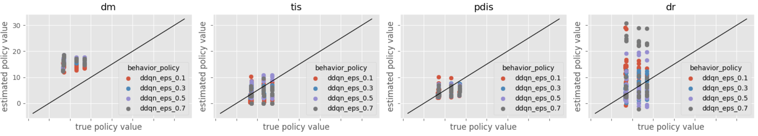
Figure 15: Example of comparing the true and estimated policy value for validation with multiple logged datasets.

References

- Brockman et al. [2016] Greg Brockman, Vicki Cheung, Ludwig Pettersson, Jonas Schneider, John Schulman, Jie Tang, and Wojciech Zaremba. Openai gym. arXiv preprint arXiv:1606.01540, 2016.
- Chandak et al. [2021] Yash Chandak, Scott Niekum, Bruno da Silva, Erik Learned-Miller, Emma Brunskill, and Philip S Thomas. Universal off-policy evaluation. In Advances in Neural Information Processing Systems, volume 34, pages 27475–27490, 2021.
- Doroudi et al. [2017] Shayan Doroudi, Philip S Thomas, and Emma Brunskill. Importance sampling for fair policy selection. Grantee Submission, 2017.
- Dudík et al. [2011] Miroslav Dudík, John Langford, and Lihong Li. Doubly robust policy evaluation and learning. In Proceedings of the 28th International Conference on International Conference on Machine Learning, ICML’11, page 1097–1104, Madison, WI, USA, 2011. Omnipress. ISBN 9781450306195.
- Fu et al. [2021] Justin Fu, Mohammad Norouzi, Ofir Nachum, George Tucker, Ziyu Wang, Alexander Novikov, Mengjiao Yang, Michael R. Zhang, Yutian Chen, Aviral Kumar, Cosmin Paduraru, Sergey Levine, and Thomas Paine. Benchmarks for deep off-policy evaluation. In International Conference on Learning Representations, 2021.
- Gauci et al. [2018] Jason Gauci, Edoardo Conti, Yitao Liang, Kittipat Virochsiri, Yuchen He, Zachary Kaden, Vivek Narayanan, Xiaohui Ye, Zhengxing Chen, and Scott Fujimoto. Horizon: Facebook’s open source applied reinforcement learning platform. arXiv preprint arXiv:1811.00260, 2018.
- Hanna et al. [2017] Josiah Hanna, Peter Stone, and Scott Niekum. Bootstrapping with models: Confidence intervals for off-policy evaluation. In Proceedings of the AAAI Conference on Artificial Intelligence, volume 31, 2017.
- Huang et al. [2021] Audrey Huang, Liu Leqi, Zachary Lipton, and Kamyar Azizzadenesheli. Off-policy risk assessment in contextual bandits. In Advances in Neural Information Processing Systems, volume 34, pages 23714–23726, 2021.
- Huang et al. [2022] Audrey Huang, Liu Leqi, Zachary Lipton, and Kamyar Azizzadenesheli. Off-policy risk assessment for markov decision processes. In roceedings of the 25th International Conference on Artificial Intelligence and Statistics, pages 5022–5050, 2022.
- Jeunen et al. [2022] Olivier Jeunen, Sean Murphy, and Ben Allison. Learning to bid with auctiongym. In KDD 2022 Workshop on Artificial Intelligence for Computational Advertising (AdKDD), 2022. URL https://www.amazon.science/publications/learning-to-bid-with-auctiongym.
- Jiang and Li [2016] Nan Jiang and Lihong Li. Doubly robust off-policy value evaluation for reinforcement learning. In Proceedings of the 33rd International Conference on Machine Learning, volume 48, pages 652–661. PMLR, 2016.
- Kallus and Uehara [2019] Nathan Kallus and Masatoshi Uehara. Intrinsically efficient, stable, and bounded off-policy evaluation for reinforcement learning. In Advances in Neural Information Processing Systems, 2019.
- Kallus and Uehara [2020] Nathan Kallus and Masatoshi Uehara. Double reinforcement learning for efficient off-policy evaluation in markov decision processes. Journal of Machine Learning Research, 21(167), 2020.
- Kallus and Zhou [2018] Nathan Kallus and Angela Zhou. Policy evaluation and optimization with continuous treatments. In Proceedings of the 21st International Conference on Artificial Intelligence and Statistics, volume 84, pages 1243–1251. PMLR, 2018.
- Kiyohara et al. [2021] Haruka Kiyohara, Kosuke Kawakami, and Yuta Saito. Accelerating offline reinforcement learning application in real-time bidding and recommendation: Potential use of simulation. arXiv preprint arXiv:2109.08331, 2021.
- Kiyohara et al. [2022] Haruka Kiyohara, Yuta Saito, Tatsuya Matsuhiro, Yusuke Narita, Nobuyuki Shimizu, and Yasuo Yamamoto. Doubly robust off-policy evaluation for ranking policies under the cascade behavior model. In Proceedings of the 15th ACM International Conference on Web Search and Data Mining, page 487–497, 2022.
- Kiyohara et al. [2023a] Haruka Kiyohara, Ren Kishimoto, Kosuke Kawakami, Ken Kobayashi, Kazuhide Nakata, and Yuta Saito. Towards assessing and benchmarking risk-return tradeoff of off-policy evaluation. arXiv preprint arXiv:2311.18207, 2023a.
- Kiyohara et al. [2023b] Haruka Kiyohara, Masatoshi Uehara, Yusuke Narita, Nobuyuki Shimizu, Yasuo Yamamoto, and Yuta Saito. Off-policy evaluation of ranking policies under diverse user behavior. In Proceedings of the 29th ACM SIGKDD Conference on Knowledge Discovery and Data Mining, pages 1154–1163, 2023b.
- Kurenkov and Kolesnikov [2022] Vladislav Kurenkov and Sergey Kolesnikov. Showing your offline reinforcement learning work: Online evaluation budget matters. In Proceedings of the 39th International Conference on Machine Learning, pages 11729–11752. PMLR, 2022.
- Le et al. [2019] Hoang Le, Cameron Voloshin, and Yisong Yue. Batch policy learning under constraints. In Proceedings of the 36th International Conference on Machine Learning, volume 97, pages 3703–3712. PMLR, 2019.
- Lee et al. [2022] Jonathan N Lee, George Tucker, Ofir Nachum, Bo Dai, and Emma Brunskill. Oracle inequalities for model selection in offline reinforcement learning. In Advances in Neural Information Processing Systems, volume 35, pages 28194–28207, 2022.
- Levine et al. [2020] Sergey Levine, Aviral Kumar, George Tucker, and Justin Fu. Offline reinforcement learning: Tutorial, review, and perspectives on open problems. arXiv preprint arXiv:2005.01643, 2020.
- Liang et al. [2018] Eric Liang, Richard Liaw, Robert Nishihara, Philipp Moritz, Roy Fox, Ken Goldberg, Joseph Gonzalez, Michael Jordan, and Ion Stoica. Rllib: Abstractions for distributed reinforcement learning. In International Conference on Machine Learning, pages 3053–3062. PMLR, 2018.
- Liu et al. [2018] Qiang Liu, Lihong Li, Ziyang Tang, and Dengyong Zhou. Breaking the curse of horizon: Infinite-horizon off-policy estimation. Advances in Neural Information Processing Systems, 31, 2018.
- Matsushima et al. [2021] Tatsuya Matsushima, Hiroki Furuta, Yutaka Matsuo, Ofir Nachum, and Shixiang Gu. Deployment-efficient reinforcement learning via model-based offline optimization. In International Conference on Learning Representations, 2021.
- Metelli et al. [2021] Alberto Maria Metelli, Alessio Russo, and Marcello Restelli. Subgaussian and differentiable importance sampling for off-policy evaluation and learning. In Advances in Neural Information Processing Systems, volume 34, 2021.
- Nachum et al. [2019a] Ofir Nachum, Yinlam Chow, Bo Dai, and Lihong Li. Dualdice: Behavior-agnostic estimation of discounted stationary distribution corrections. Advances in Neural Information Processing Systems, 32, 2019a.
- Nachum et al. [2019b] Ofir Nachum, Bo Dai, Ilya Kostrikov, Yinlam Chow, Lihong Li, and Dale Schuurmans. Algaedice: Policy gradient from arbitrary experience. arXiv preprint arXiv:1912.02074, 2019b.
- Paine et al. [2020] Tom Le Paine, Cosmin Paduraru, Andrea Michi, Caglar Gulcehre, Konrad Zolna, Alexander Novikov, Ziyu Wang, and Nando de Freitas. Hyperparameter selection for offline reinforcement learning. arXiv preprint arXiv:2007.09055, 2020.
- Precup et al. [2000] Doina Precup, Richard S. Sutton, and Satinder P. Singh. Eligibility traces for off-policy policy evaluation. In Proceedings of the 17th International Conference on Machine Learning, page 759–766, 2000.
- Qin et al. [2021] Rongjun Qin, Songyi Gao, Xingyuan Zhang, Zhen Xu, Shengkai Huang, Zewen Li, Weinan Zhang, and Yang Yu. Neorl: A near real-world benchmark for offline reinforcement learning. arXiv preprint arXiv:2102.00714, 2021.
- Rohde et al. [2018] David Rohde, Stephen Bonner, Travis Dunlop, Flavian Vasile, and Alexandros Karatzoglou. Recogym: A reinforcement learning environment for the problem of product recommendation in online advertising. arXiv preprint arXiv:1808.00720, 2018.
- Saito and Joachims [2022] Yuta Saito and Thorsten Joachims. Off-policy evaluation for large action spaces via embeddings. arXiv preprint arXiv:2202.06317, 2022.
- Saito et al. [2021a] Yuta Saito, Shunsuke Aihara, Megumi Matsutani, and Yusuke Narita. Open bandit dataset and pipeline: Towards realistic and reproducible off-policy evaluation. In Thirty-fifth Conference on Neural Information Processing Systems Datasets and Benchmarks Track, 2021a.
- Saito et al. [2021b] Yuta Saito, Takuma Udagawa, Haruka Kiyohara, Kazuki Mogi, Yusuke Narita, and Kei Tateno. Evaluating the robustness of off-policy evaluation. In Proceedings of the 15th ACM Conference on Recommender Systems, page 114–123, 2021b.
- Saito et al. [2023] Yuta Saito, Qingyang Ren, and Thorsten Joachims. Off-policy evaluation for large action spaces via conjunct effect modeling. arXiv preprint arXiv:2305.08062, 2023.
- Seno and Imai [2021] Takuma Seno and Michita Imai. d3rlpy: An offline deep reinforcement learning library. arXiv preprint arXiv:2111.03788, 2021.
- Sharpe [1998] William F Sharpe. The sharpe ratio. Streetwise–the Best of the Journal of Portfolio Management, 3:169–185, 1998.
- Su et al. [2020] Yi Su, Pavithra Srinath, and Akshay Krishnamurthy. Adaptive estimator selection for off-policy evaluation. In Prooceedings of the 38th International Conference on Machine Learning, pages 9196–9205. PMLR, 2020.
- Swaminathan and Joachims [2015] Adith Swaminathan and Thorsten Joachims. The Self-normalized Estimator for Counterfactual Learning. In Advances in Neural Information Processing Systems, pages 3231–3239, 2015.
- Tarasov et al. [2022] Denis Tarasov, Alexander Nikulin, Dmitry Akimov, Vladislav Kurenkov, and Sergey Kolesnikov. CORL: Research-oriented deep offline reinforcement learning library. In 3rd Offline RL Workshop: Offline RL as a ”Launchpad”, 2022. URL https://openreview.net/forum?id=SyAS49bBcv.
- Thomas and Brunskill [2016] Philip Thomas and Emma Brunskill. Data-efficient off-policy policy evaluation for reinforcement learning. In Proceedings of the 33rd International Conference on Machine Learning, volume 48, pages 2139–2148. PMLR, 2016.
- Thomas et al. [2015a] Philip Thomas, Georgios Theocharous, and Mohammad Ghavamzadeh. High confidence policy improvement. In Proceedings of the 32th International Conference on Machine Learning, pages 2380–2388, 2015a.
- Thomas et al. [2015b] Philip S Thomas, Georgios Theocharous, and Mohammad Ghavamzadeh. High-Confidence Off-Policy Evaluation. AAAI, pages 3000–3006, 2015b.
- Udagawa et al. [2023] Takuma Udagawa, Haruka Kiyohara, Yusuke Narita, Yuta Saito, and Kei Tateno. Policy-adaptive estimator selection for off-policy evaluation. In Proceedings of the AAAI Conference on Artificial Intelligence, volume 37, pages 10025–10033, 2023.
- Uehara et al. [2020] Masatoshi Uehara, Jiawei Huang, and Nan Jiang. Minimax weight and q-function learning for off-policy evaluation. In International Conference on Machine Learning, pages 9659–9668. PMLR, 2020.
- Uehara et al. [2022a] Masatoshi Uehara, Haruka Kiyohara, Andrew Bennett, Victor Chernozhukov, Nan Jiang, Nathan Kallus, Chengchun Shi, and Wen Sun. Future-dependent value-based off-policy evaluation in pomdps. arXiv preprint arXiv:2207.13081, 2022a.
- Uehara et al. [2022b] Masatoshi Uehara, Chengchun Shi, and Nathan Kallus. A review of off-policy evaluation in reinforcement learning. arXiv preprint arXiv:2212.06355, 2022b.
- Voloshin et al. [2019] Cameron Voloshin, Hoang M Le, Nan Jiang, and Yisong Yue. Empirical study of off-policy policy evaluation for reinforcement learning. arXiv preprint arXiv:1911.06854, 2019.
- Wang et al. [2021] Kai Wang, Zhene Zou, Qilin Deng, Yue Shang, Minghao Zhao, Runze Wu, Xudong Shen, Tangjie Lyu, and Changjie Fan. Rl4rs: A real-world benchmark for reinforcement learning based recommender system. arXiv preprint arXiv:2110.11073, 2021.
- Wu et al. [2023] Runzhe Wu, Masatoshi Uehara, and Wen Sun. Distributional offline policy evaluation with predictive error guarantees. arXiv preprint arXiv:2302.09456, 2023.
- Xie and Jiang [2021] Tengyang Xie and Nan Jiang. Batch value-function approximation with only realizability. In Proceedings of the 38th International Conference on Machine Learning, pages 11404–11413. PMLR, 2021.
- Xu et al. [2022] Yang Xu, Chengchun Shi, Shikai Luo, Lan Wang, and Rui Song. Quantile off-policy evaluation via deep conditional generative learning. arXiv preprint arXiv:2212.14466, 2022.
- Yang et al. [2020] Mengjiao Yang, Ofir Nachum, Bo Dai, Lihong Li, and Dale Schuurmans. Off-policy evaluation via the regularized lagrangian. Advances in Neural Information Processing Systems, 33:6551–6561, 2020.
- Yuan et al. [2021] Christina Yuan, Yash Chandak, Stephen Giguere, Philip S Thomas, and Scott Niekum. Sope: Spectrum of off-policy estimators. Advances in Neural Information Processing Systems, 34:18958–18969, 2021.
- Zhang et al. [2020a] Ruiyi Zhang, Bo Dai, Lihong Li, and Dale Schuurmans. Gendice: Generalized offline estimation of stationary values. International Conference on Learning Representations, 2020a.
- Zhang et al. [2020b] Shangtong Zhang, Bo Liu, and Shimon Whiteson. Gradientdice: Rethinking generalized offline estimation of stationary values. In Proceedings of the 37th International Conference on Machine Learning, pages 11194–11203. PMLR, 2020b.
- Zhang and Jiang [2021] Siyuan Zhang and Nan Jiang. Towards hyperparameter-free policy selection for offline reinforcement learning. Advances in Neural Information Processing Systems, 34:12864–12875, 2021.