SMaRt: Improving GANs with Score Matching Regularity

Abstract

Generative adversarial networks (GANs) usually struggle in learning from highly diverse data, whose underlying manifold is complex. In this work, we revisit the mathematical foundations of GANs, and theoretically reveal that the native adversarial loss for GAN training is insufficient to fix the problem of subsets with positive Lebesgue measure of the generated data manifold lying out of the real data manifold. Instead, we find that score matching serves as a promising solution to this issue thanks to its capability of persistently pushing the generated data points towards the real data manifold. We thereby propose to improve the optimization of GANs with score matching regularity (SMaRt). Regarding the empirical evidences, we first design a toy example to show that training GANs by the aid of a ground-truth score function can help reproduce the real data distribution more accurately, and then confirm that our approach can consistently boost the synthesis performance of various state-of-the-art GANs on real-world datasets with pre-trained diffusion models acting as the approximate score function. For instance, when training Aurora on the ImageNet $64\times 64$ dataset, we manage to improve FID from 8.87 to 7.11, on par with the performance of one-step consistency model. The source code will be made public.

Wenping WangtexamFellow, IEEE Yong-Jin Liu^†thuSenior Member, IEEE

Mengfei Xiaxmf20@mails.tsinghua.edu.cn Yujun Shenshenyujun0302@gmail.com Ceyuan Yanglimbo0066@gmail.com Ran Yiranyi@sjtu.edu.cn Wenping Wangwenping@tamu.edu

1 Introduction

During the last period, deep generative models have made significant improvements in a variety of domains, such as data generation (Karras et al., 2020, 2021; Ho et al., 2020; Song et al., 2020; Dhariwal & Nichol, 2021; Karras et al., 2022) and image editing (Shen et al., 2019; Shen & Zhou, 2020; Zhu et al., 2023a; Meng et al., 2022; Couairon et al., 2023). It is well recognized that, recent generative models, such as DALL$\cdot$E 2 (Ramesh et al., 2022), Stable Diffusion (Rombach et al., 2021), GigaGAN (Kang et al., 2023), and Aurora (Zhu et al., 2023b), have achieved unprecedented capability improvement of high-resolution image generation, among which, diffusion probabilistic models (DPMs) are the most prominent. DPMs leverage the diffusion and denoising processes. Their intrinsic intricate knowledge of data distribution and strong capability to scale up, make DPMs the most successful and potential options for generative modeling. The other paradigm now dominant, generative adversarial networks (GANs) (Goodfellow et al., 2014; Brock et al., 2019), introduce an implicit modeling. Despite enabling expeditious generation, GANs are usually criticized for unsatisfactory visual quality and limited diversity when compared with DPMs, making GANs seem to be falling from grace on image generation tasks. However, GAN remains a worthy tool considering its good performance on single-domain datasets (e.g., human faces) (Karras et al., 2020, 2021) and its interpretable latent space (Shen et al., 2019; Zhu et al., 2023a).

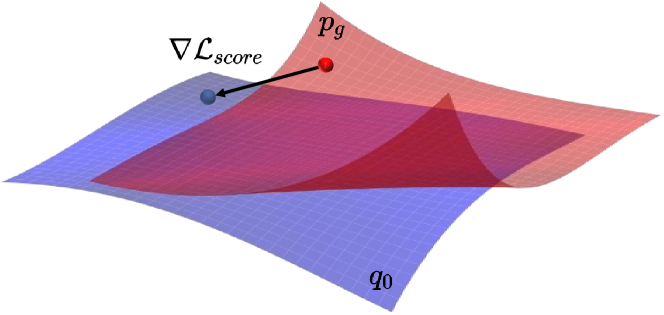
Figure 1: Motivation scheme of SMaRt. Red and blue surfaces denote the generated and real data manifolds, respectively. The positive-Lebesgue-measure subset of out-of-manifold generated samples leads to non-optimal constant generator loss, annihilating the gradient for generator. However, the proposed score matching regularity ($\mathcal{L}_{score}$ in Eq. 10) provides complementary guidance, urging such a subset to move towards the real data manifold. In this case, generator loss regains to exert effective guidance aiding the generator distribution to converge to the real one.

In this work, we dig into the mathematical foundations of GANs and reveal the necessary and sufficient conditions of optimality of generator loss. We argue in Theorem 3.1 that positive-Lebesgue-measure difference sets of generated data manifold over real data manifold lead to constant but non-optimal generator loss, which annihilates the gradient and cancels effective guidance. However, such non-optimality largely harms the synthesis performance, demonstrated in Theorem 3.2. More seriously, the gradient vanishing occurs frequently in practice. Note that, real and generated data can be referred to as low-dimensional manifolds embedded in the high-dimensional pixel space, leading to the probability of transversal intersection or non-intersection equaling to 1 (Arjovsky & Bottou, 2016). This indicates that the difference set of generated data over real data manifold almost always has positive Lebesgue measure.

Based on the above analyses, we are devoted to designing an effective methodology to tackle this obstacle. We propose a universal solution, Score Matching Regularity, namely SMaRt, leveraging score matching to facilitate GAN training. The theoretical foundation is that, score matching pushes out-of-data-manifold generated sample towards the data manifold throughout, summarized in Theorem 3.3 and demonstrated in Fig. 1. Revealing this rigorous mathematical foundation, SMaRt persistently provides gradient for generator, enforcing the generator distribution to support only on the data manifold. Afterwards, the generator loss could regain the correct and effective guidance towards data distribution. Our motivation is intuitive – GAN loss focuses only on the generated and real data manifold, while the score matching on the whole space manages to serve as a regularity to facilitate GAN training. By doing so, we succeed on alleviating the gradient vanishing issue. Hence, our work offers a new perspective on improving GAN performance. Given the rapid improvement in seminal works, the editing on a well-studied latent space (Shen et al., 2019; Shen & Zhou, 2020; Zhu et al., 2023a), and the strong compatibility with the involvement of 3D-aware image synthesis (Chan et al., 2022, 2021; Gao et al., 2022; Gu et al., 2022; Shi et al., 2023, 2022), we believe that our work could encourage more studies in the field of visual content generation.

2 Related work

GANs and improved GAN training. GANs (Goodfellow et al., 2014) have become one of the main paradigms of generative models for high-quality image generation. Thanks to the rapidly and significantly improvement on the sampling quality (Karras et al., 2018, 2019, 2020, 2021; Kang et al., 2023; Zhu et al., 2023b), GANs are introduced to various downstream applications, including text-to-image synthesis (Reed et al., 2016; Kang et al., 2023; Zhu et al., 2023b), and image-to-image translation (Isola et al., 2017; Rai & Shukla, 2017; Huang et al., 2018; Lee et al., 2018; Park et al., 2019, 2020). In particular, style-based GANs (Karras et al., 2019, 2020) have shown impressive ability on single-domain datasets (e.g., human faces) and interpretable latent space (Shen et al., 2019; Zhu et al., 2023a). However, GANs severely suffer from the famous “gradient vanishing” (Arjovsky & Bottou, 2016) dilemma, restricting further development of synthesis quality and diversity. To this end, WGAN (Arjovsky et al., 2017) replaces the native KL-divergence with Wasserstein distance as the GAN loss, inspired by optimal transportation. Besides, progressive training has been widely studied in GAN literature (Chan et al., 2021; Karras et al., 2018, 2019), thanks to its efficacy in improving training stability and efficiency. Theoretically, SMaRt can be considered as a regularity compatible with existing GAN training strategies, effectively addressing the GAN training obstacles.

DPMs and efficient DPM sampling. DPMs (Sohl-Dickstein et al., 2015; Ho et al., 2020; Song et al., 2020) introduce a novel scheme of generative model, trained by optimizing the variational lower bound. Benefiting from this breakthrough, DPMs achieve high generation fidelity, and even beat GANs on image generation. Therefore, various works followed with promising results, including video synthesis (Ho et al., 2022), conditional generation (Choi et al., 2021; Huang et al., 2023), and text-to-image synthesis (Ramesh et al., 2022; Rombach et al., 2021; Saharia et al., 2022). However, DPM employs an iterative refinement via thousands of denoising steps, suffers from a slow inference speed. Efficient DPMs sampling explores shorter denoising trajectories rather than the complete reverse process, while ensuring the synthesis performance. One representative category introduces knowledge distillation (Salimans & Ho, 2022; Luhman & Luhman, 2021; Song et al., 2023; Luo et al., 2023). Despite respectable performance with 1 step (Song et al., 2023; Luo et al., 2023), they require expensive distillation stages, leading to poor applicability.

3 Method

3.1 Background on GANs and DPMs

Denote by $\mathbf{x}$ the training data with an unknown distribution $q_{0}(\mathbf{x})$. GANs involve a generator $G$ and a discriminator $D$, to map random noise $\mathbf{z}$ to sample and discriminate real or generated samples, respectively (Goodfellow et al., 2014). Formally, GANs endeavor to achieve Nash equilibrium via the following two losses:

$$\mathcal{L}_{G} =-\mathbb{E}_{\mathbf{z}}[\log D(G(\mathbf{z}))],$$ (1)

$$\mathcal{L}_{D} =-\mathbb{E}_{\mathbf{x}}[\log D(\mathbf{x})]-\mathbb{E}_{\mathbf{z}}[\log(1-D(G(\mathbf{z})))],$$ (2)

where $\mathbf{z}$ is random noise embedded in the latent space.

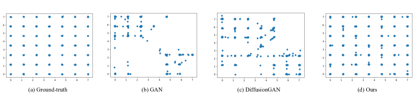
Figure 2: Visualization of discrete distribution example. The demonstrated toy data is simulated by a mixture of 49 2-dimensional Gaussian distributions with extremely low variance. Each data sample is a 2-dimensional feature tensor. Following (Wang et al., 2022), we train a small GAN model, whose generator and discriminator are both parameterized by MLPs, with two 128-unit hidden layers and LeakyReLU activation functions. We show (a) the true data samples, (b) the generated samples from vanilla GAN, (c) the generated samples from DiffusionGAN (Wang et al., 2022), and (d) the generated samples from our SMaRt. As is demonstrated, vanilla GAN and DiffusionGAN fail to address all samples onto the data manifold discretely, i.e., the generated samples tends to be continuous and out of the grids. As a comparison, our SMaRt can successfully synthesize discrete samples, whose distribution coincides with the ground-truth.

On the other hand, DPMs (Sohl-Dickstein et al., 2015; Song et al., 2020; Ho et al., 2020) define a forward diffusion process $\{\mathbf{x}_{t}\}_{t\in[0,T]},T>0$ by gradually corrupting the initial information of $\mathbf{x}$ with Gaussian noise, such that for any timestep $0<t\leqslant T$, we have the transition distribution:

$$q_{0|t}(\mathbf{x}_{t}|\mathbf{x})=\mathcal{N}(\mathbf{x}_{t};\alpha_{t}\mathbf{x},\sigma_{t}^{2}\mathbf{I}),$$ (3)

where $\alpha_{t},\sigma_{t}>0$ are differentiable functions of $t$. The selection of $\alpha_{t},\sigma_{t}$ is referred to as the noise schedule. Denote by $q_{t}(\mathbf{x}_{t})$ the marginal distribution of $\mathbf{x}_{t}$, DPM fits $\mathcal{N}(\mathbf{x}_{T};\mathbf{0},\sigma^{2}\mathbf{I})$ with $q_{T}(\mathbf{x}_{T})$ for some $\sigma>0$, and the signal-to-noise-ratio (SNR) $\alpha_{t}^{2}/\sigma_{t}^{2}$ is strictly decreasing w.r.t. $t$ (Kingma et al., 2021). DPMs utilize the noise prediction model $\bm{\epsilon}_{\theta}(\mathbf{x}_{t},t)$, to approximate the score function from $\mathbf{x}_{t}$, where the optimal parameter $\theta^{*}$ can be optimized by the objective below through denoising score matching:

$$\theta^{*}=\mathop{\arg\min}_{\theta}\mathbb{E}_{\mathbf{x},\bm{\epsilon},t}\left[\|\bm{\epsilon}_{\theta}(\mathbf{x}_{t},t)-\bm{\epsilon}\|_{2}^{2}\right],$$ (4)

where $\bm{\epsilon}\sim\mathcal{N}(\mathbf{0},\mathbf{I})$, $\mathbf{x}_{t}=\alpha_{t}\mathbf{x}+\sigma_{t}\bm{\epsilon}$, and $t\sim\mathcal{U}[0,T]$.

3.2 Revisiting GAN Training

We first delve into the theory of GANs, trying to analyze the dilemma encountered by GANs with deep findings. Recall that when GANs achieve the Nash equilibrium, we have the two equalities about $q_{0}$ and generator distribution $p_{g}$:

$$D(\mathbf{x})=\frac{q_{0}(\mathbf{x})}{q_{0}(\mathbf{x})+p_{g}(\mathbf{x})},\quad p_{g}(\mathbf{x})=q_{0}(\mathbf{x}),$$ (5)

and $\mathcal{L}_{G}$ in Eq. 1 reaches the minimum $\log 2$. However, we have the following theorem describing gradient vanishing.

Theorem 3.1.

Let $A,B$ be sets with positive $d$-dimensional Lebesgue measure, i.e., $\mu_{d}(A)>0,\mu_{d}(B)>0$. Denote by $q_{A}(\mathbf{x}),q_{B}(\mathbf{x})$ two distributions supported on $A,B$, respectively, i.e., $\mathrm{supp}\;q_{A}=\{\mathbf{x}\mid q_{A}(\mathbf{x})\neq 0\}=A$, $\mathrm{supp}\;q_{B}=B$. Let $X\backslash Y=\{\mathbf{x}\mid\mathbf{x}\in X\text{ and }\mathbf{x}\notin Y\}$. When $D$ reaches the optimality, and if $\mu_{d}(A\backslash B)>0$, then

$$-\int q_{A}(\mathbf{x})\log\frac{q_{B}(\mathbf{x})}{q_{A}(\mathbf{x})+q_{B}(\mathbf{x})}\mathrm{d}\mathbf{x}=+\infty.$$ (6)

Let $q_{0}=q_{B},p_{g}=q_{A}$, Theorem 3.1 claims that $\mathcal{L}_{G}$ remains non-optimal constant and provides no gradient to the generator when the generated data has positive-measure difference set over data manifold. Empirically, real data is embedded in a very low-dimensional manifold in the pixel space, and so is the generated data due to the low-dimensional latent space. The two manifolds will almost always have zero-measure intersection (transversal intersection or non-intersection), and thus positive-measure difference set, since $A\backslash B=A\backslash(A\cap B)$. Therefore, Theorem 3.1 is almost always the case during GAN training.

We then turn to the necessary and sufficient conditions of optimality of generator loss, which is summarized below.

Theorem 3.2.

Following the settings in Theorem 3.1, when $D$ reaches the optimality, the following inequality reaches its optimality if and only if $\mu_{d}(A\backslash B)=\mu_{d}(B\backslash A)=0$, and $\mu_{d}(\{\mathbf{x}\mid q_{A}|_{A\cap B}(\mathbf{x})\neq q_{B}|_{A\cap B}(\mathbf{x})\})=0$.

$$-\int q_{A}(\mathbf{x})\log\frac{q_{B}(\mathbf{x})}{q_{A}(\mathbf{x})+q_{B}(\mathbf{x})}\mathrm{d}\mathbf{x} \geqslant\log 2,$$ (7)

where $f|_{X}(\mathbf{x})$ equals to $f(\mathbf{x})$ on $X$ and 0 out of $X$.

Theorem 3.2 gives an insight of the behavior of the generator, i.e., the generator’s correctly imitating data distribution is equivalent to the optimality of the generator loss. Combining with Theorem 3.1, we can conclude that once $(\mathrm{supp}\;p_{g})\backslash(\mathrm{supp}\;q_{0})$ has positive Lebesgue measure, the generator distribution has not coincided with the ground-truth yet but will no longer be updated. To be more detailed, the generator loss fails due to the low dimension of the data and generator manifolds. The two manifolds will almost always have zero-measure intersection (transversal intersection or non-intersection) (Arjovsky & Bottou, 2016), and thus positive-measure difference set.

We further give a toy example designed on discrete data distribution. The toy data is simulated by a mixture of 49 2-dimensional Gaussian distributions with extremely low variance. Each data sample is a 2-dimensional feature tensor. To demonstrate the poor performance on discrete data distribution, following (Wang et al., 2022), we train a small GAN, whose generator and discriminator are both parameterized by MLPs, with two 128-unit hidden layers and LeakyReLU activation functions. As shown in Fig. 2, vanilla GAN and DiffusionGAN cannot handle the discrete data, synthesizing continuous samples. In other words, vanilla GAN tends to synthesizing a positive-measure set of samples out of the data manifold (i.e., the 49 grids). This directly leads to gradient vanishing due to Theorem 3.1.

3.3 Score Matching Regularity

Unlike GANs, DPMs focus on the whole pixel space via score matching, due to the forward diffusion process, which diffuses the data distribution to the normal distribution. Thanks to this, score matching manages to serve as a regularity to facilitate GAN training.

We first delve into the theory of score matching. Recall that in the DDIM sampling process (Song et al., 2021), one first calculates $\hat{\bm{\epsilon}_{t}}=\bm{\epsilon}_{\theta}(\mathbf{x}_{t},t)$ for the intermediate noisy result $\mathbf{x}_{t}$. With this $\hat{\bm{\epsilon}_{t}}$, one can predict an approximation $\hat{\mathbf{x}}_{0}$ of the clean data. However, this predicted $\hat{\mathbf{x}}_{0}$ is usually of poor quality, and needs further refinement by the iterative diffusion and denoising process. Formally, given a sample $\mathbf{x}$, the one-step refinement $\mathcal{R}$ process with noise $\bm{\epsilon}$ and timestep $t$ is defined as the following form:

$$\mathcal{R}(\mathbf{x},\bm{\epsilon},t):=\mathbf{x}+\frac{\sigma_{t}}{\alpha_{t}}(\bm{\epsilon}-\bm{\epsilon}_{\theta}(\alpha_{t}\mathbf{x}+\sigma_{t}\bm{\epsilon},t)).$$ (8)

Note that applying infinitely many one-step refinements is able to pulling any out-of-data-manifold point back to data manifold. We summarize this property as below.

Theorem 3.3.

Denote by $\mathrm{dist}(\mathbf{x})$ the distance between $\mathbf{x}$ and $\mathrm{supp}\;q_{0}$. For any $\mathbf{y}\notin\mathrm{supp}\;q_{0}$, define a sequence of random variables $\mathbf{y}_{0}=\mathbf{y}$, $\mathbf{y}_{k+1}=\mathcal{R}(\mathbf{y}_{k},\bm{\epsilon}_{k},t)$ with $\bm{\epsilon}_{k}\sim\mathcal{N}(\mathbf{0},\mathbf{I})$. Then $\{\mathbf{y}_{k}\}_{k=0}^{\infty}$ converges to $\mathrm{supp}\;q_{0}$, i.e.,

$$\lim_{k\rightarrow+\infty,t\rightarrow 0}\mathrm{dist}(\mathbf{y}_{k})=0.$$ (9)

Now we formally propose SMaRt, which trains GAN with an extra score matching regularity from pre-trained DPM in a plug-in sense. Let $g_{\phi}$ be the generator, we design a regularization term as below:

$$\mathcal{L}_{score}=\mathbb{E}_{\mathbf{z},\bm{\epsilon},t}[\|\bm{\epsilon}_{\theta}(\alpha_{t}g_{\phi}(\mathbf{z})+\sigma_{t}\bm{\epsilon},t)-\bm{\epsilon}\|_{2}^{2}].$$ (10)

With a loss weight $\lambda_{score}$, the total objective of generator turns out to be $\mathcal{L}_{G}+\lambda_{score}\mathcal{L}_{score}$. One can easily see that

$$\|\mathcal{R}(\mathbf{x},\bm{\epsilon},t)-\mathbf{x}\|_{2}^{2}\propto\|\bm{\epsilon}_{\theta}(\alpha_{t}\mathbf{x}+\sigma_{t}\bm{\epsilon},t)-\bm{\epsilon}\|_{2}^{2},$$ (11)

$$\mathcal{L}_{score}\propto\mathbb{E}_{\mathbf{z},\bm{\epsilon},t}[\|\mathcal{R}(g_{\phi}(\mathbf{z}),\bm{\epsilon},t)-g_{\phi}(\mathbf{z})\|_{2}^{2}].$$ (12)

According to Theorem 3.3, Eq. 12 indicates that the score matching regularity aims to narrow the distance between synthesized samples and data manifold. Therefore, when generator distribution has positive-measure difference set over data manifold (indicating gradient vanishing), for each out-of-data-manifold sample $\mathbf{x}$, $\|\mathcal{R}(\mathbf{x},\bm{\epsilon},t)-\mathbf{x}\|_{2}^{2}$ remains positive, and $\mathcal{L}_{score}$ provides gradient for generator persistently to guide $\mathbf{x}$ to lie on data manifold. Once all generated samples support on the data manifold, gradient from $\mathcal{L}_{score}$ will be annihilated. In this case, the gradient vanishing issue can be largely mitigated, and Eq. 1 will resume to supervise GAN training guaranteed by Theorem 3.2. This profound conclusion facilitates GAN training from a novel perspective.

On the other hand, serving as a regularity forcing out-of-data-manifold samples back to data manifold at a fixed and finite frequency, small $\lambda_{score}$ suggests inconspicuous guidance, weakening the functionality of SMaRt. However, when facing discrete data distribution, too strong regularity may restrict the generator distribution on only few modes, indicating that large $\lambda_{score}$ may affect synthesis diversity. Detailed ablation study of $\lambda_{score}$ is addressed in Tab. 3.

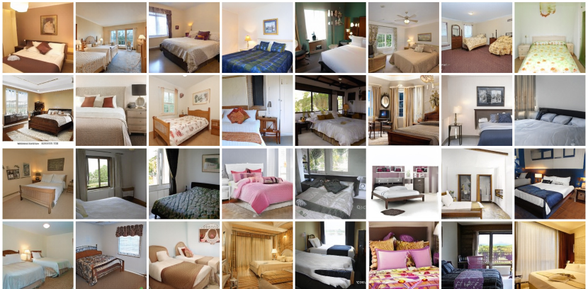
Figure 3: Diverse results generated by SMaRt upon StyleGAN2 (Karras et al., 2020) trained on LSUN Bedroom 256x256 dataset (Yu et al., 2015). We randomly sample the global latent code $\mathbf{z}$ for each image.

To take a further step, SMaRt can be generalized to conditional GANs, in which GAN loss becomes:

$$\mathcal{L}_{G} =-\mathbb{E}_{\mathbf{z},c}[\log D(G(\mathbf{z},c),c)],$$ (13)

$$\mathcal{L}_{D} =-\mathbb{E}_{\mathbf{x},c}[\log D(\mathbf{x},c)]$$

$$\qquad-\mathbb{E}_{\mathbf{z},c}[\log(1-D(G(\mathbf{z},c),c))],$$ (14)

where $c$ is the input condition. To supervise the conditional GANs using SMaRt, we simply add score matching regularity with a conditioned DPM as below:

$${}\mathcal{L}_{score}=\mathbb{E}_{\mathbf{z},\bm{\epsilon},t,c}[\|\bm{\epsilon}_{\theta}(\alpha_{t}g_{\phi}(\mathbf{z},c)+\sigma_{t}\bm{\epsilon},c,t)-\bm{\epsilon}\|_{2}^{2}].$$ (15)

We provide a theorem similar to Theorem 3.3 confirming the feasibility of SMaRt under conditional generation settings, which is addressed in Sec. A.4.

3.4 Training Strategy

As a supernumerary regularity involved time-consuming DPM, it might be challenging to efficiently and effectively plug SMaRt in native GAN training. We propose the lazy strategy and narrowed timestep interval. It is noteworthy that, even though our approach adopts the mechanisms of both adversarial learning and score matching regularity, there is no instability in the entire training process.

Lazy strategy. We propose lazy strategy, which applies the regularity less frequently than the main loss function, thus greatly diminishing the DPM computational cost. Tab. 4 studies the efficacy of the regularity under different frequencies, providing an empirically adequate strategy.

Narrowed timestep interval. Recall that the score matching regularity can be considered as guidance from DDIM refinement. Therefore, the involved timestep is attached great importance to the refinement performance. Theoretically, large timestep suggests large discretization step of the differential equation, harming the quality of the refinement. On the other hand, finite refinement steps entail that tiny timestep leads to inconspicuous refinement, since $\frac{\sigma_{t}}{\alpha_{t}}$ in Eq. 8 tends to zero. Performance comparison among different timestep interval is addressed in Tab. 3.

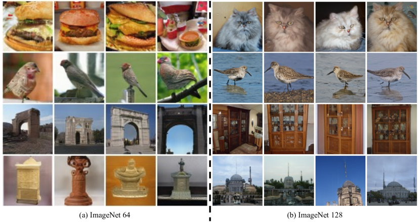
Figure 4: Diverse results generated by SMaRt upon (a) Aurora (Zhu et al., 2023b) on ImageNet 64x64 dataset (Deng et al., 2009) and (b) BigGAN (Brock et al., 2019) on ImageNet 128x128 dataset (Deng et al., 2009). We randomly sample four global latent codes $\mathbf{z}$ for each label condition $c$, demonstrated in each row.

4 Experiments

4.1 Experimental Setups

Table 1: Sample quality on CIFAR10 (Krizhevsky & Hinton, 2009). ^∗Methods that require synthetic data construction for distillation. For clearer demonstration, one-step approaches including GANs and DPMs are highlighted in gray.

rowsep=0.548pt colsep=3.0pt METHOD NFE $(\downarrow)$ FID $(\downarrow)$ IS $(\uparrow)$ ScoreSDE (Song et al., 2020) 2000 2.20 9.89 DDPM (Ho et al., 2020) 1000 3.17 9.46 LSGM (Vahdat et al., 2021) 147 2.10 – PFGM (Xu et al., 2022) 110 2.35 9.68 EDM (Karras et al., 2022) 35 1.97 – DDIM (Song et al., 2021) 50 4.67 – DDIM (Song et al., 2021) 30 6.84 – DDIM (Song et al., 2021) 10 8,23 – DPM-solver-3 (Lu et al., 2022) 12 6.03 – 3-DEIS (Zhang & Chen, 2023) 10 4.17 – UniPC (Zhao et al., 2023) 8 5.10 – UniPC (Zhao et al., 2023) 5 23.22 – Denoise Diffusion GAN (T=2) (Xiao et al., 2022) 2 4.08 9.80 PD (Salimans & Ho, 2022) 2 5.58 9.05 CT (Song et al., 2023) 2 5.83 8.85 iCT (Song & Dhariwal, 2023) 2 2.46 9.80 CD (Song et al., 2023) 2 2.93 9.75 Denoise Diffusion GAN (T=1) (Xiao et al., 2022) 1 14.60 8.93 KD^∗ (Luhman & Luhman, 2021) 1 9.36 – TDPM (Zheng et al., 2023) 1 8.91 8.65 1-ReFlow (Liu et al., 2023) 1 378.00 1.13 CT (Song et al., 2023) 1 8.70 8.49 iCT (Song & Dhariwal, 2023) 1 2.83 9.54 1-ReFlow (+distill)^∗ (Liu et al., 2023) 1 6.18 9.08 2-ReFlow (+distill)^∗ (Liu et al., 2023) 1 4.85 9.01 3-ReFlow (+distill)^∗ (Liu et al., 2023) 1 5.21 8.79 PD (Salimans & Ho, 2022) 1 8.34 8.69 CD-L2 (Song et al., 2023) 1 7.90 – CD-LPIPS (Song et al., 2023) 1 3.55 9.48 Diff-Instruct (Luo et al., 2023) 1 4.19 – AutoGAN (Gong et al., 2019) 1 12.40 8.55 E2GAN (Tian et al., 2020) 1 11.30 8.51 TransGAN (Jiang et al., 2021) 1 9.26 9.05 StyleGAN-XL (Sauer et al., 2022) 1 1.85 – Diffusion StyleGAN2 (Wang et al., 2022) 1 3.19 9.94 StyleGAN2-ADA (Karras et al., 2020) 1 2.42 9.83 StyleGAN2-ADA+Tune+DI (Luo et al., 2023) 1 2.27 10.11 StyleGAN2-ADA + SMaRt 1 2.06 10.22

Table 2: Sample quality on ImageNet (Deng et al., 2009) and LSUN Bedroom 256x256 (Yu et al., 2015). ^†Methods that utilize distillation techniques. ^‡Methods that are trained by ourselves with official implementation. For clearer demonstration, one-step approaches including GANs and DPMs are highlighted in gray.

rowsep=0.5pt colsep=1.5pt METHOD NFE $(\downarrow)$ FID $(\downarrow)$ Prec. $(\uparrow)$ Rec. $(\uparrow)$ ImageNet 64x64 PD^† (Salimans & Ho, 2022) 2 8.95 0.63 0.65 CD^† (Song et al., 2023) 2 4.70 0.69 0.64 PD^† (Salimans & Ho, 2022) 1 15.39 0.59 0.62 CD^† (Song et al., 2023) 1 6.20 0.68 0.63 ADM (Dhariwal & Nichol, 2021) 250 2.07 0.74 0.63 EDM (Karras et al., 2022) 79 2.44 0.71 0.67 DDIM (Song et al., 2021) 50 13.70 0.65 0.56 DEIS (Zhang & Chen, 2023) 10 6.65 – – CT (Song et al., 2023) 2 11.10 0.69 0.56 CT (Song et al., 2023) 1 13.00 0.71 0.47 iCT (Song & Dhariwal, 2023) 1 4.02 0.70 0.63 StyleGAN2^‡ (Karras et al., 2020) 1 21.32 0.42 0.36 StyleGAN2 + SMaRt 1 18.31 0.45 0.39 Aurora^‡ (Zhu et al., 2023b) 1 8.87 0.41 0.48 Aurora + SMaRt 1 7.11 0.42 0.49 ImageNet 128x128 ADM (Dhariwal & Nichol, 2021) 250 5.91 0.70 0.65 BigGAN^‡ (Brock et al., 2019) 1 10.76 0.73 0.29 BigGAN + SMaRt 1 9.49 0.77 0.30 LSUN Bedroom 256x256 PD^† (Salimans & Ho, 2022) 2 8.47 0.56 0.39 CD^† (Song et al., 2023) 2 5.22 0.68 0.39 PD^† (Salimans & Ho, 2022) 1 16.92 0.47 0.27 CD^† (Song et al., 2023) 1 7.80 0.66 0.34 DDPM (Ho et al., 2020) 1000 4.89 0.60 0.45 ADM (Dhariwal & Nichol, 2021) 1000 1.90 0.66 0.51 EDM (Karras et al., 2022) 79 3.57 0.66 0.45 CT (Song et al., 2023) 2 7.85 0.68 0.33 CT (Song et al., 2023) 1 16.00 0.60 0.17 PGGAN (Karras et al., 2018) 1 8.34 – – PG-SWGAN (Wu et al., 2019) 1 8.00 – – StyleGAN2 (Karras et al., 2020) 1 2.35 0.59 0.48 Diffusion StyleGAN2 (Wang et al., 2022) 1 3.65 0.60 0.32 StyleGAN2 + SMaRt 1 1.98 0.61 0.49

Datasets and baselines. We apply SMaRt to previous seminal GANs, including StyleGAN2 (Karras et al., 2020), BigGAN (Brock et al., 2019), and Aurora (Zhu et al., 2023b). We train StyleGAN2 on CIFAR10 32x32 (Krizhevsky & Hinton, 2009) and LSUN Bedroom 256x256 (Yu et al., 2015), BigGAN and Aurora on ImageNet 128x128 and 64x64 (Deng et al., 2009), respectively.

Evaluation metrics. We draw 50,000 samples for Fréchet Inception Distance (FID) (Heusel et al., 2017) to evaluate the fidelity of the synthesized images. Inception Score (IS) (Salimans et al., 2016) measures how well a model captures the full ImageNet class distribution while still convincingly producing individual samples from a single class. Finally, we use Improved Precision (Prec.) and Recall (Rec.) (Kynkäänniemi et al., 2019) to separately measure sample fidelity (Precision) and diversity (Recall).

Implementation details. We train SMaRt using PyTorch (Paszke et al., 2019) with NVIDIA Tesla A100 GPUs. With abundant powerful pre-trained DPMs as expertise, we choose the state-of-the-art ADM (Dhariwal & Nichol, 2021) and EDM (Karras et al., 2022). We use the pre-trained ADM and EDM provided in the official implementation. Regarding GANs, we use the third-party implementation of StyleGAN2 (Karras et al., 2020) under Hammer (Shen et al., 2022) and officially implemented BigGAN (Brock et al., 2019) and Aurora (Zhu et al., 2023b).

4.2 Toy Example on Self-designed Dataset

We conduct experiments of generation task on the discrete data distribution. The toy data is simulated by a mixture of 49 2-dimensional Gaussian distributions with extremely low variance. Following (Wang et al., 2022), we train a small GAN model, whose generator and discriminator are both parameterized by MLPs, with two 128-unit hidden layers and LeakyReLU activation functions. The training results are shown in Fig. 2. Note that the vanilla GAN exhibits poor synthesis discreteness. By adopting the noise injection to discriminator, DiffusionGAN (Wang et al., 2022) turns to fit the distribution of noisy data, endeavoring to promote synthesis diversity. However, this compromises the synthesis quality to a certain extent, making the generated samples less discrete. As a comparison, our SMaRt is capable of capturing the discrete distribution, confirming the feasibility by simply adding the score matching regularity. This indicates that SMaRt manages to settle the gradient vanishing by eliminating out-of-data-manifold samples.

4.3 Results on Real Datasets

Qualitative results. We showcase some results in Figs. 3 and 4. One can see that, with score matching regularity, GAN is more capable of synthesizing samples addressed on data manifold, especially the conditional generation in Fig. 4, getting out of the dilemma of gradient vanishing. It is also noteworthy that SMaRt promotes the synthesis diversity to a certain extent, since generator loss provides more significant guidance on the data manifold.

Quantitative comparison. Besides the exhibited qualitative results, we also provide quantitative comparison between baseline and SMaRt-improving version on various state-of-the-art GANs, conveying an overall picture of its capability of promoting generation performance. In Tabs. 2 and 2, we report the evaluation results on three different data domains, including CIFAR10, LSUN Bedroom 256x256, and ImageNet. We can tell that SMaRt achieves performance improvement on the three datasets.

Table 3: Ablation study of narrowed timestep interval and loss weight $\lambda_{score}$ using StyleGAN2-ADA (Karras et al., 2020) on CIFAR10 (Krizhevsky & Hinton, 2009).

rowsep=1.0pt colsep=9pt Config. Baseline Freq. $=8$ $t\in[5,15]$ $t\in[40,60]$ $t\in[40,60]$ $t\in[90,110]$ $t\in[225,275]$ $\lambda_{score}=0.01$ $\lambda_{score}=0.01$ $\lambda_{score}=0.025$ $\lambda_{score}=0.05$ $\lambda_{score}=0.1$ FID ($\downarrow$) 2.42 2.17 2.06 2.08 2.12 2.11 IS ($\uparrow$) 9.83 10.15 10.22 10.20 10.21 10.26

4.4 Analyses

Ablation study. We conduct comprehensive ablation study to convey a direct and clear picture of the efficacy of the score matching regularity under different settings. We can conclude from Tab. 3 that both too large (e.g., $t\in[225,275]$) and too tiny (e.g., $t\in[5,15]$) timestep interval negatively influences the synthesis performance, which is consistent with the analysis of the narrowed timestep interval in Sec. 3.4. Besides, large $\lambda_{score}$ (e.g., $\lambda_{score}=0.025$) harms both FID and IS performance, also coinciding with the previous analysis in Sec. 3.4. As reported in Tab. 4, the behavior of too frequent or infrequent regularization is similar to that of large or tiny $\lambda_{score}$, respectively.

Computational cost comparison. As one of the representative one-step generation paradigms, Consistent Distillation (CD) (Song et al., 2023) distills intricate knowledge from pre-trained DPMs. We report in Tab. 5 the FID performance, total training iterations, training time for one iteration, and number of used GPUs, respectively. In spite of achieving respectable performance, CD involves more training iterations and GPUs than both baseline and SMaRt-improving version of Aurora (Zhu et al., 2023b). As a comparison, SMaRt slightly slows down the training speed of the baseline model (about 1.6 times training time cost).

Latent interpolation. Latent space interpolation is widely studied in the seminal literature (Brock et al., 2019; Karras et al., 2019, 2020), which aims to verify the generative ability of the GANs. It is well recognized that GANs possess semantically continuous and extremely smooth latent spaces (Ali et al., 2020; Wu et al., 2021; Shen et al., 2019). We demonstrate the results of latent interpolation within $\mathcal{W}$ space (i.e., the disentangled latent space) in Fig. 5, in which the observation coincides with the common conclusion. As a comparison, we show the interpolation of Consistency Model (CM) (Song et al., 2023), which is also a one-step synthesis paradigm. As shown in Fig. 5, CM fails to synthesize correct results with interpolated latent codes, indicating the poor continuity of the latent space and thus the difficulty for editing and other downstream applications.

Table 4: Ablation study of frequency of lazy strategy using StyleGAN2-ADA (Karras et al., 2020) on CIFAR10 (Krizhevsky & Hinton, 2009).

rowsep=1.2pt colsep=6.0pt Config. Baseline $t\in[40,60]$, $\lambda_{score}=0.01$ Freq. $=4$ Freq. $=8$ Freq. $=16$ FID ($\downarrow$) 2.42 2.24 2.06 2.07 IS ($\uparrow$) 9.83 10.19 10.22 10.22

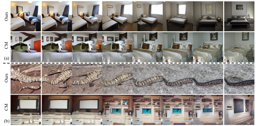
Figure 5: Visualization of latent interpolation results on (a) LSUN Bedroom 256x256, and (b) ImageNet 64x64. We employ StyleGAN2 (Karras et al., 2020) and Consistency Model (CM) (Song et al., 2023) on LSUN Bedroom 256x256 dataset, interpolating in the disentangled latent space. As for interpolation on ImageNet 64x64 dataset, we introduce Aurora (Zhu et al., 2023b) and CM (Song et al., 2023). We fix the label condition $c$, and only interpolate in the disentangled latent space $\mathcal{W}$. It is noteworthy that both StyleGAN2 and Aurora are strongly capable of synthesizing correct interpolation results, due to the extremely smooth and well-studied latent spaces. However, CM fails to generate interpolation results, due to poor semantic continuity in the latent space.

4.5 Discussion

It is the gradient vanishing of GANs that restricts the downstream applications, leaving GANs lacking further research such as text-to-image synthesis. Therefore, we believe our SMaRt is attached to great importance. In spite of the great success on facilitating training of GANs, our proposed algorithm has several potential limitations. As a supplemental regularity for GAN training, its efficacy depends highly on the choice of the narrowed timestep interval, and the loss weight $\lambda_{score}$. Although we conduct extensive and convincing ablation studies and provide an empirically adequate solution, the optimality of such a strategy is currently unexplored. Besides, due to additionally involving the score matching via noise prediction model, SMaRt introduces the lazy strategy to diminishing time cost. However, this still slightly slows down the training speed of GANs (about 1.6 times training time cost). Therefore, how to determine the optimal frequency, narrowed timestep interval, and loss weight of score matching according to different model settings and data domains will be an interesting avenue for future research.

Table 5: Comparison of computational cost between Aurora (Zhu et al., 2023b) and Consistency Distillation (CD) on ImageNet 64x64 (Deng et al., 2009). We report FID, total training iterations, time for one iteration, and number of GPUs, respectively.

rowsep=1.0pt colsep=1.8pt Method FID ($\downarrow$) Training Iter. Time # GPUs Aurora (Zhu et al., 2023b) 8.87 256k 3.3s 16 Aurora+SMaRt 7.11 256k 2.9s 32 CD (Song et al., 2023) 6.20 600k – 64

5 Conclusion

In this paper, we analyze and alleviate the gradient vanishing of GANs by delving into the background mathematical foundation of GAN loss. We theoretically point out a novel perspective to facilitate GAN training. Drawing lessons from score matching, we propose SMaRt, a plug-in algorithm which significantly punishes gradient vanishing. We provide a proof that score matching serving as a regularity provides supernumerary guidance enforcing out-of-data-manifold samples by generator towards data manifold. Under this circumstance, generator loss is more capable of guiding generator distribution to converge to data distribution. We conduct comprehensive experiments to demonstrate significant improvement of synthesis quality on a variety of datasets and baseline models.

Broader impact. The proposed approach represents a significant advancement in the field of GAN synthesis, which is both a fundamental and practical problem. The introduction of the score matching regularity from pre-trained DPMs has greatly enhanced the capacity for handling gradient vanishing, making GAN training more stable. However, this technique may also facilitate the creation of fake content, such as Deepfake, which could have negative consequences. We want to emphasize that we strongly oppose the misuse of this approach to violate security and privacy issues. The negative impact of such misuse can be mitigated by the development of deep fake detection technology.

Appendix

Appendix A Proofs and derivations

In this section, we will prove the theorems claimed in the main manuscript. First, we emphasize a property in Riemann integral, which is attached great importance to the proofs and derivations in the sequel.

Proposition A.1.

Let $f$ be a Lebesgue-measurable function, and $Z$ be a set with zero Lebesgue measure. The integral of $f$ on $Z$ is 0, i.e.,

$$\int_{Z}f(\mathbf{x})\mathrm{d}\mathbf{x}=0.$$ (16)

A.1 Proof of Theorem 3.1

Theorem A.2.

Let $A,B\subset\mathbb{R}^{d}$ with positive Lebesgue measure, i.e., $\mu_{d}(A)>0,\mu_{d}(B)>0$. Denote by $q_{A}(\mathbf{x}),q_{B}(\mathbf{x})$ two distributions supported on $A,B$, respectively, i.e., $\mathrm{supp}\;q_{A}=\{\mathbf{x}\mid q_{A}(\mathbf{x})\neq 0\}=A$, $\mathrm{supp}\;q_{B}=B$. Let $X\backslash Y=\{\mathbf{x}\mid\mathbf{x}\in X\text{ and }\mathbf{x}\notin Y\}$. When $D$ reaches the optimality, and if $\mu_{d}(A\backslash B)>0$, then

$$-\int q_{A}(\mathbf{x})\log\frac{q_{B}(\mathbf{x})}{q_{A}(\mathbf{x})+q_{B}(\mathbf{x})}\mathrm{d}\mathbf{x}=+\infty.$$ (17)

Proof.

We first divide the union of $A$ and $B$ as below:

$$A\cup B=(A\backslash B)\coprod(B\backslash A)\coprod(A\cap B),$$ (18)

where $\coprod$ represents the disjoint union. Note that $q_{A}(\mathbf{x})\log\frac{q_{B}(\mathbf{x})}{q_{A}(\mathbf{x})+q_{B}(\mathbf{x})}=0$ for $\mathbf{x}\notin A\cup B$ and $\mathbf{x}\in B\backslash A$. Therefore

$$-\int q_{A}(\mathbf{x})\log\frac{q_{B}(\mathbf{x})}{q_{A}(\mathbf{x})+q_{B}(\mathbf{x})}\mathrm{d}\mathbf{x}$$ (19)

$$= -\int_{A\cup B}q_{A}(\mathbf{x})\log\frac{q_{B}(\mathbf{x})}{q_{A}(\mathbf{x})+q_{B}(\mathbf{x})}\mathrm{d}\mathbf{x}$$ (20)

$$= -\int_{A\backslash B}q_{A}(\mathbf{x})\log\frac{q_{B}(\mathbf{x})}{q_{A}(\mathbf{x})+q_{B}(\mathbf{x})}\mathrm{d}\mathbf{x}$$

$$\qquad-\int_{B\backslash A}q_{A}(\mathbf{x})\log\frac{q_{B}(\mathbf{x})}{q_{A}(\mathbf{x})+q_{B}(\mathbf{x})}\mathrm{d}\mathbf{x}$$

$$\qquad-\int_{A\cap B}q_{A}(\mathbf{x})\log\frac{q_{B}(\mathbf{x})}{q_{A}(\mathbf{x})+q_{B}(\mathbf{x})}\mathrm{d}\mathbf{x}$$ (21)

$$\geqslant -\int_{A\backslash B}q_{A}(\mathbf{x})\log\frac{q_{B}(\mathbf{x})}{q_{A}(\mathbf{x})+q_{B}(\mathbf{x})}\mathrm{d}\mathbf{x}+0+0$$ (22)

$$= +\infty,$$ (23)

where $-\int_{A\cap B}q_{A}(\mathbf{x})\log\frac{q_{B}(\mathbf{x})}{q_{A}(\mathbf{x})+q_{B}(\mathbf{x})}\mathrm{d}\mathbf{x}\geqslant-\sup_{\mathbf{x}\in A\cap B}\log\frac{q_{B}(\mathbf{x})}{q_{A}(\mathbf{x})+q_{B}(\mathbf{x})}(\int_{A\cap B}q_{A}(\mathbf{x})\mathrm{d}\mathbf{x})\geqslant 0$ is by the property of Riemann integral. And Eq. 23 is due to $\mu_{d}(A\backslash B)>0$ and $\frac{q_{B}(\mathbf{x})}{q_{A}(\mathbf{x})+q_{B}(\mathbf{x})}=0$ on $A\backslash B$. ∎

A.2 Proof of Theorem 3.2

Theorem A.3.

Following the settings in Theorem 3.1, when $D$ reaches the optimality, the following inequality reaches its optimal if and only if $\mu_{d}(A\backslash B)=\mu_{d}(B\backslash A)=0$, and $\mu_{d}(\{\mathbf{x}\mid q_{A}|_{A\cap B}(\mathbf{x})\neq q_{B}|_{A\cap B}(\mathbf{x})\})=0$.

$$-\int q_{A}(\mathbf{x})\log\frac{q_{B}(\mathbf{x})}{q_{A}(\mathbf{x})+q_{B}(\mathbf{x})}\mathrm{d}\mathbf{x} \geqslant\log 2,$$ (24)

where

$$f|_{X}(\mathbf{x})=\begin{cases}&f(\mathbf{x})\quad\text{if }\mathbf{x}\in X,\\ &0\quad\text{otherwise.}\end{cases}$$ (25)

Proof.

We first divide the union of $A$ and $B$ as below:

$$A\cup B=(A\backslash B)\coprod(B\backslash A)\coprod(A\cap B),$$ (26)

where $\coprod$ represents the disjoint union. Then one can divide the integral into three parts:

$$-\int q_{A}(\mathbf{x})\log\frac{q_{B}(\mathbf{x})}{q_{A}(\mathbf{x})+q_{B}(\mathbf{x})}\mathrm{d}\mathbf{x} =-\int_{A\backslash B}q_{A}(\mathbf{x})\log\frac{q_{B}(\mathbf{x})}{q_{A}(\mathbf{x})+q_{B}(\mathbf{x})}\mathrm{d}\mathbf{x}$$ (27)

$$\qquad-\int_{B\backslash A}q_{A}(\mathbf{x})\log\frac{q_{B}(\mathbf{x})}{q_{A}(\mathbf{x})+q_{B}(\mathbf{x})}\mathrm{d}\mathbf{x}$$ (28)

$$\qquad-\int_{A\cap B}q_{A}(\mathbf{x})\log\frac{q_{B}(\mathbf{x})}{q_{A}(\mathbf{x})+q_{B}(\mathbf{x})}\mathrm{d}\mathbf{x}.$$ (29)

When $\mu_{d}(A\backslash B)=\mu_{d}(B\backslash A)=0$, by Proposition A.1, we have

$$-\int_{A\backslash B}q_{A}(\mathbf{x})\log\frac{q_{B}(\mathbf{x})}{q_{A}(\mathbf{x})+q_{B}(\mathbf{x})}\mathrm{d}\mathbf{x} =0$$ (30)

$$-\int_{B\backslash A}q_{A}(\mathbf{x})\log\frac{q_{B}(\mathbf{x})}{q_{A}(\mathbf{x})+q_{B}(\mathbf{x})}\mathrm{d}\mathbf{x} =0.$$ (31)

Let $Z=\{\mathbf{x}\mid q_{A}|_{A\cap B}(\mathbf{x})\neq q_{B}|_{A\cap B}(\mathbf{x})\}$. Note that $Z\subseteq A\cap B$, since $q_{A}|_{A\cap B}=q_{B}|_{A\cap B}\equiv 0$ outside $A\cap B$. When $\mu_{d}(Z)=0$, then we have

$$-\int_{A\cap B}q_{A}(\mathbf{x})\log\frac{q_{B}(\mathbf{x})}{q_{A}(\mathbf{x})+q_{B}(\mathbf{x})}\mathrm{d}\mathbf{x}$$ (32)

$$= -\int_{(A\cap B)\backslash Z}q_{A}(\mathbf{x})\log\frac{1}{2}\mathrm{d}\mathbf{x}-\int_{Z}q_{A}(\mathbf{x})\log\frac{q_{B}(\mathbf{x})}{q_{A}(\mathbf{x})+q_{B}(\mathbf{x})}\mathrm{d}\mathbf{x}-\int_{Z}q_{A}(\mathbf{x})\log\frac{1}{2}\mathrm{d}\mathbf{x}$$ (33)

$$= -\int_{A\cap B}q_{A}(\mathbf{x})\log\frac{1}{2}\mathrm{d}\mathbf{x}+0$$ (34)

$$= -\int_{A\cap B}q_{A}(\mathbf{x})\log\frac{1}{2}\mathrm{d}\mathbf{x}-\int_{A\backslash B}q_{A}(\mathbf{x})\log\frac{1}{2}\mathrm{d}\mathbf{x}$$ (35)

$$= -\int_{A}q_{A}(\mathbf{x})\log\frac{1}{2}\mathrm{d}\mathbf{x}=\log 2,$$ (36)

where Eqs. 33 and 35 are due to $\mu_{d}(Z)=\mu_{d}(A\backslash B)=0$ and Proposition A.1.

On the other hand, when the inequality reaches its minimum, by the definition of the support set, we have $q_{A}|_{B\backslash A}\equiv 0$, and $q_{B}|_{A\backslash B}\equiv 0$. Therefore, we have $\frac{q_{B}}{q_{A}+q_{B}}|_{A\backslash B}\equiv 0$, and

$$-\int_{B\backslash A}q_{A}(\mathbf{x})\log\frac{q_{B}(\mathbf{x})}{q_{A}(\mathbf{x})+q_{B}(\mathbf{x})}\mathrm{d}\mathbf{x}=0.$$ (37)

If $\mu_{d}(A\backslash B)>0$, then

$$-\int_{A\backslash B}q_{A}(\mathbf{x})\log\frac{q_{B}(\mathbf{x})}{q_{A}(\mathbf{x})+q_{B}(\mathbf{x})}\mathrm{d}\mathbf{x}=+\infty,$$ (38)

which contradicts with the optimality. Hence we prove that $\mu_{d}(A\backslash B)=0$.

Let $Z=\{\mathbf{x}\mid q_{A}|_{A\cap B}(\mathbf{x})\neq q_{B}|_{A\cap B}(\mathbf{x})\}$. Then $Z\subseteq A\cap B$ since $q_{A}|_{A\cap B}=q_{B}|_{A\cap B}\equiv 0$ outside $A\cap B$. We can then deduce that

$$-\int q_{A}(\mathbf{x})\log\frac{q_{B}(\mathbf{x})}{q_{A}(\mathbf{x})+q_{B}(\mathbf{x})}\mathrm{d}\mathbf{x}$$ (39)

$$= -\int_{A\cap B}q_{A}(\mathbf{x})\log\frac{q_{B}(\mathbf{x})}{q_{A}(\mathbf{x})+q_{B}(\mathbf{x})}\mathrm{d}\mathbf{x}-\int_{A\backslash B}q_{A}(\mathbf{x})\log\frac{q_{B}(\mathbf{x})}{q_{A}(\mathbf{x})+q_{B}(\mathbf{x})}\mathrm{d}\mathbf{x}$$ (40)

$$= -\int_{A\cap B}q_{A}(\mathbf{x})\log\frac{q_{B}(\mathbf{x})}{q_{A}(\mathbf{x})+q_{B}(\mathbf{x})}\mathrm{d}\mathbf{x}$$ (41)

$$= -\int_{(A\cap B)\backslash Z}q_{A}(\mathbf{x})\log\frac{q_{B}(\mathbf{x})}{q_{A}(\mathbf{x})+q_{B}(\mathbf{x})}\mathrm{d}\mathbf{x}-\int_{Z}q_{A}(\mathbf{x})\log\frac{q_{B}(\mathbf{x})}{q_{A}(\mathbf{x})+q_{B}(\mathbf{x})}\mathrm{d}\mathbf{x}$$ (42)

$$= \log 2\left(\int_{(A\cap B)\backslash Z}q_{A}(\mathbf{x})\mathrm{d}\mathbf{x}\right)-\int_{Z}q_{A}(\mathbf{x})\log\frac{q_{B}(\mathbf{x})}{q_{A}(\mathbf{x})+q_{B}(\mathbf{x})}\mathrm{d}\mathbf{x}$$ (43)

$$= \log 2\left(\int_{(A\cap B)\backslash Z}q_{A}(\mathbf{x})\mathrm{d}\mathbf{x}+\int_{(A\backslash B)\backslash Z}q_{A}(\mathbf{x})\mathrm{d}\mathbf{x}\right)-\int_{Z}q_{A}(\mathbf{x})\log\frac{q_{B}(\mathbf{x})}{q_{A}(\mathbf{x})+q_{B}(\mathbf{x})}\mathrm{d}\mathbf{x}$$ (44)

$$= \log 2\left(\int_{A\backslash Z}q_{A}(\mathbf{x})\mathrm{d}\mathbf{x}\right)-\int_{Z}q_{A}(\mathbf{x})\log\frac{q_{B}(\mathbf{x})}{q_{A}(\mathbf{x})+q_{B}(\mathbf{x})}\mathrm{d}\mathbf{x},$$ (45)

where Eqs. 41 and 44 are due to $\mu_{d}((A\backslash B)\backslash Z)\leqslant\mu_{d}(A\backslash B)=0$ and Proposition A.1. Suppose $\mu_{d}(Z)>0$, then $C_{A}=\int_{Z}q_{A}(\mathbf{x})\mathrm{d}\mathbf{x}>0,C_{B}=\int_{Z}q_{B}(\mathbf{x})\mathrm{d}\mathbf{x}>0$. By the definition of $Z$ and $\mu_{d}(A\backslash B)=0$, we have

$$C_{A} =\int_{Z}q_{A}(\mathbf{x})\mathrm{d}\mathbf{x}+\left(\int_{(A\cap B)\backslash Z}q_{A}(\mathbf{x})\mathrm{d}\mathbf{x}-\int_{(A\cap B)\backslash Z}q_{B}(\mathbf{x})\mathrm{d}\mathbf{x}\right)+\int_{A\backslash B}q_{A}(\mathbf{x})\mathrm{d}\mathbf{x}-\int_{A\backslash B}q_{B}(\mathbf{x})\mathrm{d}\mathbf{x}$$ (46)

$$=\int_{A\cap B}q_{A}(\mathbf{x})\mathrm{d}\mathbf{x}-\int_{(A\cap B)\backslash Z}q_{B}(\mathbf{x})\mathrm{d}\mathbf{x}+\int_{A\backslash B}q_{A}(\mathbf{x})\mathrm{d}\mathbf{x}-\int_{A\backslash B}q_{B}(\mathbf{x})\mathrm{d}\mathbf{x}$$ (47)

$$=\int_{A}q_{A}(\mathbf{x})\mathrm{d}\mathbf{x}-\int_{(A\cap B)\backslash Z}q_{B}(\mathbf{x})\mathrm{d}\mathbf{x}-\int_{A\backslash B}q_{B}(\mathbf{x})\mathrm{d}\mathbf{x}$$ (48)

$$\geqslant\int_{A}q_{B}(\mathbf{x})\mathrm{d}\mathbf{x}-\int_{(A\cap B)\backslash Z}q_{B}(\mathbf{x})\mathrm{d}\mathbf{x}-\int_{A\backslash B}q_{B}(\mathbf{x})\mathrm{d}\mathbf{x}$$ (49)

$$=\int_{Z}q_{B}(\mathbf{x})\mathrm{d}\mathbf{x}=C_{B},$$ (50)

where Eq. 46 is due to $q_{A}=q_{B}$ on $(A\cap B)\backslash Z$, and $\mu_{d}(A\backslash B)=0$ with Proposition A.1.

Then we have

$$-\int_{Z}q_{A}(\mathbf{x})\log\frac{q_{B}(\mathbf{x})}{q_{A}(\mathbf{x})+q_{B}(\mathbf{x})}\mathrm{d}\mathbf{x}$$ (51)

$$= -C_{A}\int_{Z}\frac{1}{C_{A}}q_{A}(\mathbf{x})\log\frac{\frac{1}{C_{A}}q_{B}(\mathbf{x})}{\frac{1}{C_{A}}q_{A}(\mathbf{x})+\frac{1}{C_{A}}q_{B}(\mathbf{x})}\mathrm{d}\mathbf{x}$$ (52)

$$\geqslant -C_{A}\int_{Z}\frac{1}{C_{A}}q_{A}(\mathbf{x})\log\frac{\frac{1}{C_{B}}q_{B}(\mathbf{x})}{\frac{1}{C_{A}}q_{A}(\mathbf{x})+\frac{1}{C_{B}}q_{B}(\mathbf{x})}\mathrm{d}\mathbf{x}.$$ (53)

Note that $\int_{Z}\frac{1}{C_{A}}q_{A}(\mathbf{x})\mathrm{d}\mathbf{x}=\int_{Z}\frac{1}{C_{B}}q_{B}(\mathbf{x})\mathrm{d}\mathbf{x}=1$, one can rewrite $q_{A}^{\prime}=\frac{1}{C_{A}}q_{A},q_{B}^{\prime}=\frac{1}{C_{B}}q_{B},$ then we have

$$-C_{A}\int_{Z}\frac{1}{C_{A}}q_{A}(\mathbf{x})\log\frac{\frac{1}{C_{B}}q_{B}(\mathbf{x})}{\frac{1}{C_{A}}q_{A}(\mathbf{x})+\frac{1}{C_{B}}q_{B}(\mathbf{x})}\mathrm{d}\mathbf{x}$$ (54)

$$= -C_{A}\int_{Z}q_{A}^{\prime}(\mathbf{x})\log\frac{q_{B}^{\prime}(\mathbf{x})}{q_{A}^{\prime}(\mathbf{x})+q_{B}^{\prime}(\mathbf{x})}\mathrm{d}\mathbf{x}>C_{A}\log 2,$$ (55)

where Eq. 55 is due to the property of generator loss on two distinct nonzero distributions. Therefore, we have the contradiction:

$$-\int q_{A}(\mathbf{x})\log\frac{q_{B}(\mathbf{x})}{q_{A}(\mathbf{x})+q_{B}(\mathbf{x})}\mathrm{d}\mathbf{x}$$ (56)

$$= \log 2\left(\int_{A\backslash Z}q_{A}(\mathbf{x})\mathrm{d}\mathbf{x}\right)-\int_{Z}q_{A}(\mathbf{x})\log\frac{q_{B}(\mathbf{x})}{q_{A}(\mathbf{x})+q_{B}(\mathbf{x})}\mathrm{d}\mathbf{x}$$ (57)

$$> \log 2\left(\int_{A\backslash Z}q_{A}(\mathbf{x})\mathrm{d}\mathbf{x}\right)+C_{A}\log 2$$ (58)

$$= \log 2\left(\int_{A\backslash Z}q_{A}(\mathbf{x})\mathrm{d}\mathbf{x}\right)+\log 2\left(\int_{Z}q_{A}(\mathbf{x})\mathrm{d}\mathbf{x}\right)$$ (59)

$$= \log 2\left(\int_{A}q_{A}(\mathbf{x})\mathrm{d}\mathbf{x}\right)=\log 2,$$ (60)

which indicates that $\mu_{d}(Z)=0$.

Finally, it suffices to show $\mu_{d}(B\backslash A)=0$. If $\mu_{d}(B\backslash A)>0$, then $\int_{B\backslash A}q_{B}(\mathbf{x})\mathrm{d}\mathbf{x}>0$

$$C_{B} =\int_{A}q_{B}(\mathbf{x})\mathrm{d}\mathbf{x}-\int_{(A\cap B)\backslash Z}q_{B}(\mathbf{x})\mathrm{d}\mathbf{x}-\int_{A\backslash B}q_{B}(\mathbf{x})\mathrm{d}\mathbf{x}$$ (61)

$$=\left(\int_{A\backslash B}q_{B}(\mathbf{x})\mathrm{d}\mathbf{x}+\int_{A\cap B}q_{B}(\mathbf{x})\mathrm{d}\mathbf{x}\right)-\int_{(A\cap B)\backslash Z}q_{B}(\mathbf{x})\mathrm{d}\mathbf{x}-\int_{A\backslash B}q_{B}(\mathbf{x})\mathrm{d}\mathbf{x}$$ (62)

$$=\int_{A\cap B}q_{B}(\mathbf{x})\mathrm{d}\mathbf{x}-\int_{(A\cap B)\backslash Z}q_{B}(\mathbf{x})\mathrm{d}\mathbf{x}-\int_{A\backslash B}q_{B}(\mathbf{x})\mathrm{d}\mathbf{x}$$ (63)

$$=\left(\int_{B}q_{B}(\mathbf{x})\mathrm{d}\mathbf{x}-\int_{B\backslash A}q_{B}(\mathbf{x})\mathrm{d}\mathbf{x}\right)-\int_{(A\cap B)\backslash Z}q_{B}(\mathbf{x})\mathrm{d}\mathbf{x}-\int_{A\backslash B}q_{B}(\mathbf{x})\mathrm{d}\mathbf{x}$$ (64)

$$<\int_{B}q_{B}(\mathbf{x})\mathrm{d}\mathbf{x}-\int_{(A\cap B)\backslash Z}q_{B}(\mathbf{x})\mathrm{d}\mathbf{x}-\int_{A\backslash B}q_{B}(\mathbf{x})\mathrm{d}\mathbf{x}$$ (65)

$$=\int_{A}q_{A}(\mathbf{x})\mathrm{d}\mathbf{x}-\int_{(A\cap B)\backslash Z}q_{B}(\mathbf{x})\mathrm{d}\mathbf{x}-\int_{A\backslash B}q_{B}(\mathbf{x})\mathrm{d}\mathbf{x}$$ (66)

$$=\int_{A}q_{A}(\mathbf{x})\mathrm{d}\mathbf{x}-\int_{(A\cap B)\backslash Z}q_{A}(\mathbf{x})\mathrm{d}\mathbf{x}=C_{A},$$ (67)

where Eqs. 63 and 67 is due to $\mu_{d}(A\backslash B)=0$ with Proposition A.1 and $q_{A}=q_{B}$ on $(A\cap B)\backslash Z$. Then we have

$$-\int_{Z}q_{A}(\mathbf{x})\log\frac{q_{B}(\mathbf{x})}{q_{A}(\mathbf{x})+q_{B}(\mathbf{x})}\mathrm{d}\mathbf{x}$$ (68)

$$> -C_{A}\int_{Z}\frac{1}{C_{A}}q_{A}(\mathbf{x})\log\frac{\frac{1}{C_{B}}q_{B}(\mathbf{x})}{\frac{1}{C_{A}}q_{A}(\mathbf{x})+\frac{1}{C_{B}}q_{B}(\mathbf{x})}\mathrm{d}\mathbf{x}$$ (69)

$$= -C_{A}\int_{Z}q_{A}^{\prime}(\mathbf{x})\log\frac{q_{B}^{\prime}(\mathbf{x})}{q_{A}^{\prime}(\mathbf{x})+q_{B}^{\prime}(\mathbf{x})}\mathrm{d}\mathbf{x}=C_{A}\log 2,$$ (70)

and $-\int q_{A}(\mathbf{x})\log\frac{q_{B}(\mathbf{x})}{q_{A}(\mathbf{x})+q_{B}(\mathbf{x})}\mathrm{d}\mathbf{x}>\log 2\left(\int_{A\backslash Z}q_{A}(\mathbf{x})\mathrm{d}\mathbf{x}\right)+C_{A}\log 2=\log 2$. Therefore $\mu_{d}(B\backslash A)=0$. ∎

A.3 Proof of Theorem 3.3

Theorem A.4.

Denote by $\mathrm{dist}(\mathbf{x})$ the distance between $\mathbf{x}$ and $\mathrm{supp}\;q_{0}$. For any $\mathbf{y}\notin\mathrm{supp}\;q_{0}$, define a sequence of random variable $\mathbf{y}_{0}=\mathbf{y}$, $\mathbf{y}_{k+1}=\mathcal{R}(\mathbf{y}_{k},\bm{\epsilon}_{k},t)$ with $\bm{\epsilon}_{k}\sim\mathcal{N}(\mathbf{0},\mathbf{I})$. Then the sequence $\{\mathbf{y}_{k}\}_{k=0}^{\infty}$ converges to $\mathrm{supp}\;q_{0}$, i.e.,

$$\lim_{k\rightarrow+\infty,t\rightarrow 0}\mathrm{dist}(\mathbf{y}_{k})=0.$$ (71)

Proof.

Note that $\bm{\epsilon}_{\theta}(\alpha_{t}\mathbf{x}+\sigma_{t}\bm{\epsilon},t)=-\sigma_{t}\nabla\log q_{t}(\mathbf{x}_{t})$, therefore we can rewrite the one-step refinement $\mathcal{R}$ as below:

$$\mathcal{R}(\mathbf{x},\bm{\epsilon},t) =\mathbf{x}+\frac{\sigma_{t}}{\alpha_{t}}(\bm{\epsilon}-\bm{\epsilon}_{\theta}(\alpha_{t}\mathbf{x}+\sigma_{t}\bm{\epsilon},t))$$ (72)

$$=\mathbf{x}+\frac{\sigma_{t}^{2}}{\alpha_{t}}\nabla\log q_{t}(\alpha_{t}\mathbf{x}+\sigma_{t}\bm{\epsilon})+\frac{\sigma_{t}}{\alpha_{t}}\bm{\epsilon}$$ (73)

Recall the corresponding SDE of the reverse process of DPMs

$$\mathrm{d}\mathbf{x}_{t}=f(t)\mathbf{x}_{t}\mathrm{d}t-g^{2}(t)\nabla_{\mathbf{x}_{t}}\log q_{t}(\mathbf{x}_{t})\mathrm{d}t+g(t)\mathrm{d}\mathbf{w}.$$ (74)

One can refer to $\mathcal{R}$ as a discretization of Eq. 74. Then the conclusion comes directly as a deduction of the solution to this SDE in Eq. 74, since the limit for $k\rightarrow+\infty,t\rightarrow 0$ indicates the continuous version of this SDE and cancels the discretization error. ∎

Remark A.5.

As Theorem 3.3 concludes, the sequence of refined results will converge to locate at the support of the data distribution $\mathrm{supp}\;q_{0}$. By the Cauchy’s convergence law, we claim that for arbitrarily small $\varepsilon>0$, there exists $K>0$ such that for any $k>K$, we have $\|\mathbf{y}_{k+1}-\mathbf{y}_{k}\|_{2}<\varepsilon$. This indicates that there will be no gradient when synthesized samples support on the data manifold. Otherwise, the gradient of nonzero $\|\mathbf{y}_{k+1}-\mathbf{y}_{k}\|_{2}$ will enforce the convergence of the refinement sequence towards the data manifold.

A.4 Proof of Theorem A.6

Before addressing the feasibility theorem under conditional generation setting, we first define the conditional one-step refinement as below

$$\mathcal{R}(\mathbf{x},\bm{\epsilon},c,t):=\mathbf{x}+\frac{\sigma_{t}}{\alpha_{t}}(\bm{\epsilon}-\bm{\epsilon}_{\theta}(\alpha_{t}\mathbf{x}+\sigma_{t}\bm{\epsilon},c,t)).$$ (75)

Theorem A.6.

Denote by $\mathrm{dist}(\mathbf{x},c)$ the distance between pair $(\mathbf{x},c)$ and $\mathrm{supp}\;q_{0}$. For any pair $(\mathbf{y},c)\notin\mathrm{supp}\;q_{0}$, define a sequence of random variable $\mathbf{y}_{0}=\mathbf{y}$, $\mathbf{y}_{k+1}=\mathcal{R}(\mathbf{y}_{k},\bm{\epsilon}_{k},c,t)$ with $\bm{\epsilon}_{k}\sim\mathcal{N}(\mathbf{0},\mathbf{I})$. Then the sequence $\{(\mathbf{y}_{k},c)\}_{k=0}^{\infty}$ converges to $\mathrm{supp}\;q_{0}$, i.e.,

$$\lim_{k\rightarrow+\infty,t\rightarrow 0}\mathrm{dist}(\mathbf{y}_{k},c)=0.$$ (76)

Proof.

Denote by $q_{0}^{c}(\mathbf{x})=q_{0}(\mathbf{x},c)/q(c)=q_{0}(\mathbf{x}|c)$, and by $\bm{\epsilon}_{\theta}^{c}(\mathbf{x}_{t},t)=\bm{\epsilon}_{\theta}(\mathbf{x}_{t},c,t)$ for any condition $c$, one can refer to $\bm{\epsilon}_{\theta}^{c}$ as the ground-truth noise prediction model pre-trained on the data distribution $q_{0}^{c}(\mathbf{x})$. Denote by $\mathcal{R}^{c}(\mathbf{x},\bm{\epsilon},t)=\mathcal{R}(\mathbf{x},\bm{\epsilon},c,t)$ the refinement involving $\bm{\epsilon}_{\theta}^{c}$, and by $\mathrm{dist}^{c}(\mathbf{x})=\mathrm{dist}(\mathbf{x},c)$. Then by Theorem 3.3, one can conclude that for any $\mathbf{y}\notin\mathrm{supp}\;q_{0}^{c}$, and a sequence of random variable $\mathbf{y}_{0}=\mathbf{y}$, $\mathbf{y}_{k+1}=\mathcal{R}^{c}(\mathbf{y}_{k},\bm{\epsilon}_{k},t)$ with $\bm{\epsilon}_{k}\sim\mathcal{N}(\mathbf{0},\mathbf{I})$, we have

$$\lim_{k\rightarrow+\infty,t\rightarrow 0}\mathrm{dist}(\mathbf{y}_{k},c)=\lim_{k\rightarrow+\infty,t\rightarrow 0}\mathrm{dist}^{c}(\mathbf{y}_{k})=0.$$ (77)

And by the definition of $q_{0}^{c}$, $\mathbf{y}\notin\mathrm{supp}\;q_{0}^{c}$ implies that $(\mathbf{y},c)\notin\mathrm{supp}\;q_{0}$, and $\mathbf{x}\in\mathrm{supp}\;q_{0}^{c}$ implies that $(\mathbf{x},c)\in\mathrm{supp}\;q_{0}$. ∎

Appendix B Additional Samples from SMaRt

In this section, we provide additional samples from SMaRt, including diverse synthesis (i.e., Figs. 6, 7 and 8) and latent interpolation (i.e., Figs. 9 and 10). All samples are synthesized with SMaRt upon StyleGAN2 (Karras et al., 2020) on LSUN Bedroom 256x256 (Yu et al., 2015), BigGAN (Brock et al., 2019) on ImageNet 128x128 (Deng et al., 2009) and Aurora (Zhu et al., 2023b) on ImageNet 64x64 (Deng et al., 2009), respectively.

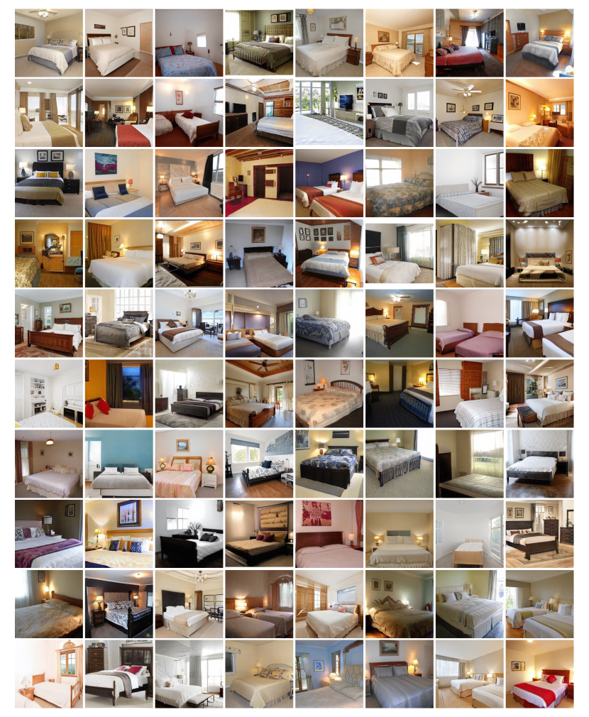
Figure 6: Diverse results generated by SMaRt upon StyleGAN2 (Karras et al., 2020) trained on LSUN Bedroom 256x256 dataset (Yu et al., 2015). We randomly sample the global latent code $\mathbf{z}$ for each image.

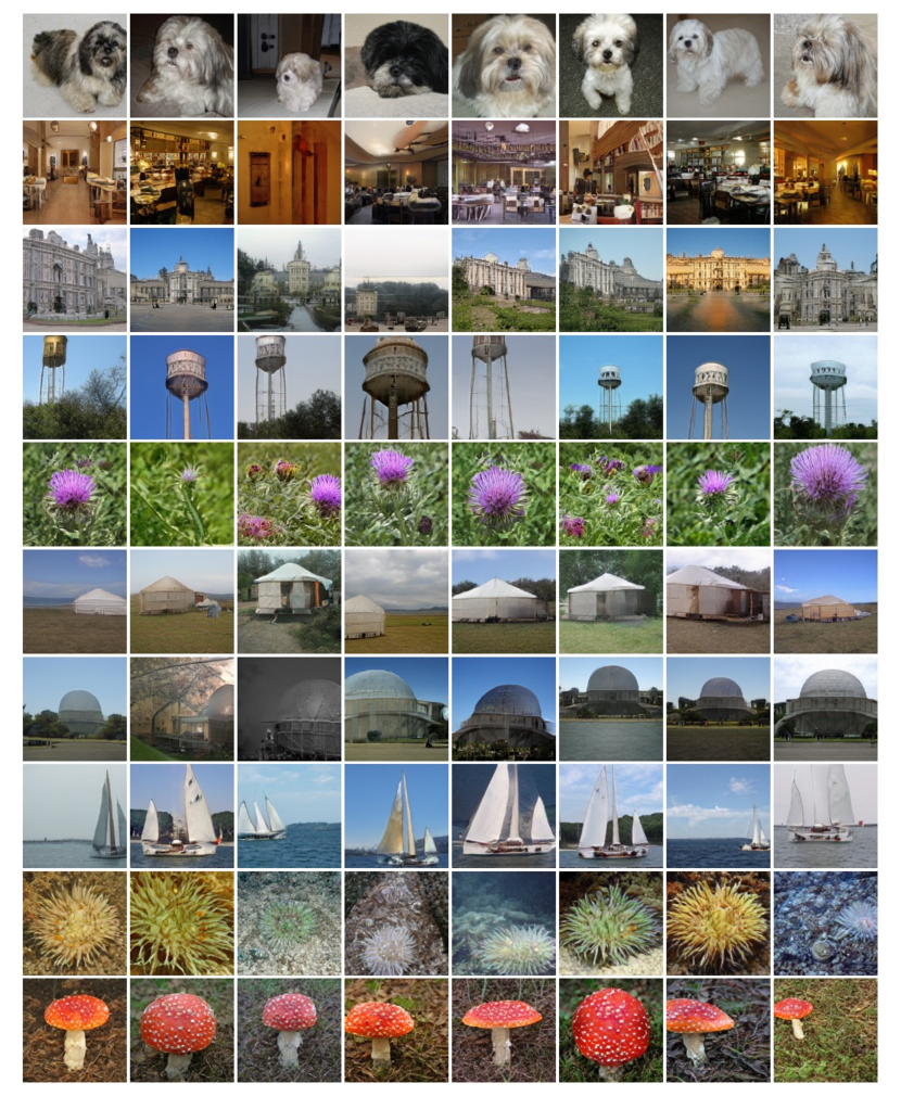
Figure 7: Diverse results generated by SMaRt upon BigGAN (Brock et al., 2019) trained on ImageNet 128x128 dataset (Deng et al., 2009) We randomly sample eight global latent codes $\mathbf{z}$ for each label condition $c$, demonstrated in each row.

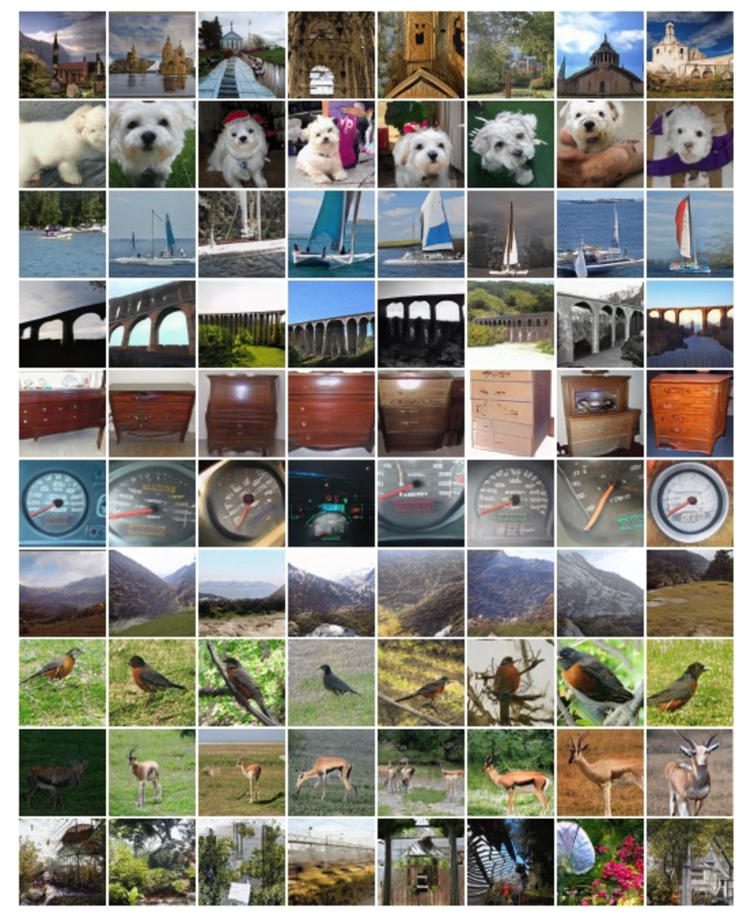
Figure 8: Diverse results generated by SMaRt upon Aurora (Zhu et al., 2023b) trained on ImageNet 64x64 dataset (Deng et al., 2009) We randomly sample eight global latent codes $\mathbf{z}$ for each label condition $c$, demonstrated in each row.

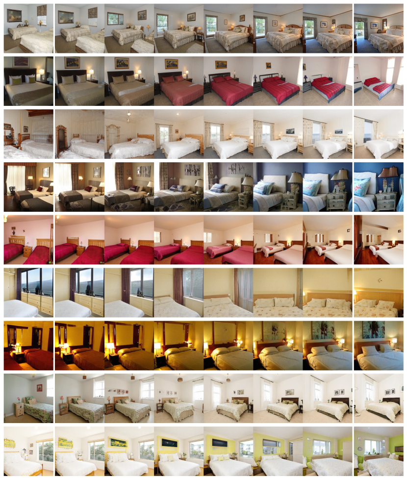
Figure 9: Interpolation between leftmost and rightmost images with linear interpolation. We apply SMaRt upon StyleGAN2 (Karras et al., 2020) on LSUN Bedroom 256x256 dataset (Yu et al., 2015), interpolating in the disentangled latent space.

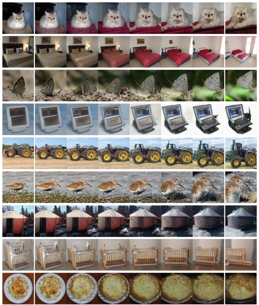
Figure 10: Interpolation between leftmost and rightmost images with linear interpolation. We apply SMaRt upon Aurora (Zhu et al., 2023b) on ImageNet 64x64 dataset (Deng et al., 2009), interpolating in the disentangled latent space by fixing the label condition.

References

- Ali et al. (2020) Ali, J., Lucy, C., and Phillip, I. On the ”steerability” of generative adversarial networks. In Int. Conf. Learn. Represent., 2020.
- Arjovsky & Bottou (2016) Arjovsky, M. and Bottou, L. Towards principled methods for training generative adversarial networks. In Int. Conf. Learn. Represent., 2016.
- Arjovsky et al. (2017) Arjovsky, M., Chintala, S., and Bottou, L. Wasserstein generative adversarial networks. In ICML, 2017.
- Brock et al. (2019) Brock, A., Donahue, J., and Simonyan, K. Large scale gan training for high fidelity natural image synthesis. In Int. Conf. Learn. Represent., 2019.
- Chan et al. (2021) Chan, E., Monteiro, M., Kellnhofer, P., Wu, J., and Wetzstein, G. pi-gan: Periodic implicit generative adversarial networks for 3d-aware image synthesis. In IEEE Conf. Comput. Vis. Pattern Recog., 2021.
- Chan et al. (2022) Chan, E. R., Lin, C. Z., Chan, M. A., Nagano, K., Pan, B., Mello, S. D., Gallo, O., Guibas, L., Tremblay, J., Khamis, S., Karras, T., and Wetzstein, G. Efficient geometry-aware 3D generative adversarial networks. In IEEE Conf. Comput. Vis. Pattern Recog., 2022.
- Choi et al. (2021) Choi, J., Kim, S., Jeong, Y., Gwon, Y., and Yoon, S. Ilvr: Conditioning method for denoising diffusion probabilistic models. In Int. Conf. Comput. Vis., pp. 14347–14356, 2021.
- Couairon et al. (2023) Couairon, G., Verbeek, J., Schwenk, H., and Cord, M. Diffedit: Diffusion-based semantic image editing with mask guidance. In Int. Conf. Learn. Represent., 2023.
- Deng et al. (2009) Deng, J., Dong, W., Socher, R., Li, L., Li, K., and Fei-Fei, L. Imagenet: A large-scale hierarchical image database. In IEEE Conf. Comput. Vis. Pattern Recog., 2009.
- Dhariwal & Nichol (2021) Dhariwal, P. and Nichol, A. Q. Diffusion models beat GANs on image synthesis. In Adv. Neural Inform. Process. Syst., 2021.
- Gao et al. (2022) Gao, J., Shen, T., Wang, Z., Chen, W., Yin, K., Li, D., Litany, O., Gojcic, Z., and Fidler, S. Get3d: A generative model of high quality 3d textured shapes learned from images. In Adv. Neural Inform. Process. Syst., 2022.
- Gong et al. (2019) Gong, X., Chang, S., Jiang, Y., and Wang, Z. Autogan: Neural architecture search for generative adversarial networks. In Int. Conf. Comput. Vis., 2019.
- Goodfellow et al. (2014) Goodfellow, I., Pouget-Abadie, J., Mirza, M., Xu, B., Warde-Farley, D., Ozair, S., Courville, A., and Bengio, Y. Generative adversarial nets. In Adv. Neural Inform. Process. Syst., 2014.
- Gu et al. (2022) Gu, J., Liu, L., Wang, P., and Theobalt, C. Stylenerf: A style-based 3d aware generator for high-resolution image synthesis. In Int. Conf. Learn. Represent., 2022.
- Heusel et al. (2017) Heusel, M., Ramsauer, H., Unterthiner, T., Nessler, B., and Hochreiter, S. Gans trained by a two time-scale update rule converge to a local nash equilibrium. In Adv. Neural Inform. Process. Syst., 2017.
- Ho et al. (2020) Ho, J., Jain, A., and Abbeel, P. Denoising diffusion probabilistic models. In Adv. Neural Inform. Process. Syst., pp. 6840–6851, 2020.
- Ho et al. (2022) Ho, J., Salimans, T., Gritsenko, A., Chan, W., Norouzi, M., and Fleet, D. J. Video diffusion models. arXiv preprint arXiv:2204.03458, 2022.
- Huang et al. (2023) Huang, L., Chen, D., Liu, Y., Yujun, S., Zhao, D., and Jingren, Z. Composer: Creative and controllable image synthesis with composable conditions. arXiv preprint arxiv:2302.09778, 2023.
- Huang et al. (2018) Huang, X., Liu, M.-Y., Belongie, S. J., and Kautz, J. Multimodal unsupervised image-to-image translation. In Eur. Conf. Comput. Vis., 2018.
- Isola et al. (2017) Isola, P., Zhu, J.-Y., Zhou, T., and Efros, A. A. Image-to-image translation with conditional adversarial networks. In IEEE Conf. Comput. Vis. Pattern Recog., pp. 5967–5976, 2017.
- Jiang et al. (2021) Jiang, Y., Chang, S., and Wang, Z. Transgan: Two pure transformers can make one strong gan, and that can scale up. In Adv. Neural Inform. Process. Syst., 2021.
- Kang et al. (2023) Kang, M., Zhu, J.-Y., Zhang, R., Park, J., Shechtman, E., Paris, S., and Park, T. Scaling up gans for text-to-image synthesis. arXiv preprint arXiv:2303.05511, 2023.
- Karras et al. (2018) Karras, T., Aila, T., Laine, S., and Lehtinen, J. Progressive growing of gans for improved quality, stability, and variation. In Int. Conf. Learn. Represent., 2018.
- Karras et al. (2019) Karras, T., Laine, S., and Aila, T. A style-based generator architecture for generative adversarial networks. In IEEE Conf. Comput. Vis. Pattern Recog., pp. 4396–4405, 2019.
- Karras et al. (2020) Karras, T., Laine, S., Aittala, M., Hellsten, J., Lehtinen, J., and Aila, T. Analyzing and improving the image quality of stylegan. In IEEE Conf. Comput. Vis. Pattern Recog., pp. 8107–8116, 2020.
- Karras et al. (2021) Karras, T., Aittala, M., Laine, S., Härkönen, E., Hellsten, J., Lehtinen, J., and Aila, T. Alias-free generative adversarial networks. In Adv. Neural Inform. Process. Syst., 2021.
- Karras et al. (2022) Karras, T., Aittala, M., Aila, T., and Laine, S. Elucidating the design space of diffusion-based generative models. In Adv. Neural Inform. Process. Syst., 2022.
- Kingma et al. (2021) Kingma, D., Salimans, T., Poole, B., and Ho, J. Variational diffusion models. In Adv. Neural Inform. Process. Syst., volume 34, pp. 21696–21707, 2021.
- Krizhevsky & Hinton (2009) Krizhevsky, A. and Hinton, G. Learning multiple layers of features from tiny images. Technical report, University of Toronto, 2009.
- Kynkäänniemi et al. (2019) Kynkäänniemi, T., Karras, T., Laine, S., Lehtinen, J., and Aila, T. Improved precision and recall metric for assessing generative models. arXiv preprint arXiv:1904.06991, 2019.
- Lee et al. (2018) Lee, H.-Y., Tseng, H.-Y., Huang, J.-B., Singh, M. K., and Yang, M.-H. Drit++: Diverse image-to-image translation via disentangled representations. In Eur. Conf. Comput. Vis., 2018.
- Liu et al. (2023) Liu, X., Gong, C., and Liu, Q. Flow straight and fast: Learning to generate and transfer data with rectified flow. In Int. Conf. Learn. Represent., 2023.
- Lu et al. (2022) Lu, C., Zhou, Y., Bao, F., Chen, J., Li, C., and Zhu, J. Dpm-solver: A fast ode solver for diffusion probabilistic model sampling in around 10 steps. In Adv. Neural Inform. Process. Syst., 2022.
- Luhman & Luhman (2021) Luhman, E. and Luhman, T. Knowledge distillation in iterative generative models for improved sampling speed. arXiv preprint arXiv:2101.02388, 2021.
- Luo et al. (2023) Luo, W., Hu, T., Zhang, S., Sun, J., Li, Z., and Zhang, Z. Diff-instruct: A universal approach for transferring knowledge from pre-trained diffusion models. arXiv preprint arXiv:2305.18455, 2023.
- Meng et al. (2022) Meng, C., He, Y., Song, Y., Song, J., Wu, J., Zhu, J.-Y., and Ermon, S. SDEdit: Guided image synthesis and editing with stochastic differential equations. In Int. Conf. Learn. Represent., 2022.
- Park et al. (2019) Park, T., Liu, M.-Y., Wang, T.-C., and Zhu, J.-Y. Semantic image synthesis with spatially-adaptive normalization. In IEEE Conf. Comput. Vis. Pattern Recog., pp. 2332–2341, 2019.
- Park et al. (2020) Park, T., Efros, A. A., Zhang, R., and Zhu, J.-Y. Contrastive learning for unpaired image-to-image translation. In Eur. Conf. Comput. Vis., 2020.
- Paszke et al. (2019) Paszke, A., Gross, S., Massa, F., Lerer, A., Bradbury, J., Chanan, G., Killeen, T., Lin, Z., Gimelshein, N., Antiga, L., et al. Pytorch: An imperative style, high-performance deep learning library. In Adv. Neural Inform. Process. Syst., 2019.
- Rai & Shukla (2017) Rai, H. and Shukla, N. Unpaired image-to-image translation using cycle-consistent adversarial networks. In Int. Conf. Comput. Vis., 2017.
- Ramesh et al. (2022) Ramesh, A., Dhariwal, P., Nichol, A., Chu, C., and Chen, M. Hierarchical text-conditional image generation with clip latents. arXiv preprint arXiv:2204.06125, 2022.
- Reed et al. (2016) Reed, S. E., Akata, Z., Yan, X., Logeswaran, L., Schiele, B., and Lee, H. Generative adversarial text to image synthesis. In Int. Conf. Mach. Learn., 2016.
- Rombach et al. (2021) Rombach, R., Blattmann, A., Lorenz, D., Esser, P., and Ommer, B. High-resolution image synthesis with latent diffusion models. IEEE Conf. Comput. Vis. Pattern Recog., 2021.
- Saharia et al. (2022) Saharia, C., Chan, W., Saxena, S., Li, L., Whang, J., Denton, E. L., Ghasemipour, S. K. S., Ayan, B. K., Mahdavi, S. S., Lopes, R. G., Salimans, T., Ho, J., Fleet, D. J., and Norouzi, M. Photorealistic text-to-image diffusion models with deep language understanding. arXiv preprint arXiv:2205.11487, 2022.
- Salimans & Ho (2022) Salimans, T. and Ho, J. Progressive distillation for fast sampling of diffusion models. In Int. Conf. Learn. Represent., 2022.
- Salimans et al. (2016) Salimans, T., Goodfellow, I. J., Zaremba, W., Cheung, V., Radford, A., and Chen, X. Improved techniques for training gans. In Adv. Neural Inform. Process. Syst., 2016.
- Sauer et al. (2022) Sauer, A., Schwarz, K., and Geiger, A. Stylegan-xl: Scaling stylegan to large diverse datasets. In SIGGRAPH, 2022.
- Shen & Zhou (2020) Shen, Y. and Zhou, B. Closed-form factorization of latent semantics in gans. In IEEE Conf. Comput. Vis. Pattern Recog., pp. 1532–1540, 2020.
- Shen et al. (2019) Shen, Y., Gu, J., Tang, X., and Zhou, B. Interpreting the latent space of gans for semantic face editing. In IEEE Conf. Comput. Vis. Pattern Recog., pp. 9240–9249, 2019.
- Shen et al. (2022) Shen, Y., Zhang, Z., Yang, D., Xu, Y., Yang, C., and Zhu, J. Hammer: An efficient toolkit for training deep models. https://github.com/bytedance/Hammer, 2022.
- Shi et al. (2022) Shi, Z., Xu, Y., Shen, Y., Zhao, D., Chen, Q., and Yeung, D.-Y. Improving 3d-aware image synthesis with a geometry-aware discriminator. In Adv. Neural Inform. Process. Syst., 2022.
- Shi et al. (2023) Shi, Z., Shen, Y., Xu, Y., Peng, S., Liao, Y., Guo, S., Chen, Q., and Yeung, D.-Y. Learning 3d-aware image synthesis with unknown pose distribution. In IEEE Conf. Comput. Vis. Pattern Recog., 2023.
- Sohl-Dickstein et al. (2015) Sohl-Dickstein, J., Weiss, E., Maheswaranathan, N., and Ganguli, S. Deep unsupervised learning using nonequilibrium thermodynamics. In Int. Conf. Mach. Learn., pp. 2256–2265. PMLR, 2015.
- Song et al. (2021) Song, J., Meng, C., and Ermon, S. Denoising diffusion implicit models. In Int. Conf. Learn. Represent., 2021.
- Song & Dhariwal (2023) Song, Y. and Dhariwal, P. Improved techniques for training consistency models. arXiv preprint arXiv:2310.14189, 2023.
- Song et al. (2020) Song, Y., Sohl-Dickstein, J., Kingma, D. P., Kumar, A., Ermon, S., and Poole, B. Score-based generative modeling through stochastic differential equations. In Int. Conf. Learn. Represent., 2020.
- Song et al. (2023) Song, Y., Dhariwal, P., Chen, M., and Sutskever, I. Consistency models. arXiv preprint arXiv:2303.01469, 2023.
- Tian et al. (2020) Tian, Y., Wang, Q., Huang, Z., Li, W., Dai, D., Yang, M., Wang, J., and Fink, O. Off-policy reinforcement learning for efficient and effective gan architecture search. In Eur. Conf. Comput. Vis., 2020.
- Vahdat et al. (2021) Vahdat, A., Kreis, K., and Kautz, J. Score-based generative modeling in latent space. In Adv. Neural Inform. Process. Syst., 2021.
- Wang et al. (2022) Wang, Z., Zheng, H., He, P., Chen, W., and Zhou, M. Diffusion-gan: Training gans with diffusion. arXiv preprint arXiv:2206.02262, 2022.
- Wu et al. (2019) Wu, J., Huang, Z., Acharya, D., Li, W., Thoma, J., Paudel, D., and Van Gool, L. Sliced wasserstein generative models. In IEEE Conf. Comput. Vis. Pattern Recog., 2019.
- Wu et al. (2021) Wu, Z., Lischinski, D., and Shechtman, E. Stylespace analysis: Disentangled controls for stylegan image generation. In IEEE Conf. Comput. Vis. Pattern Recog., 2021.
- Xiao et al. (2022) Xiao, Z., Kreis, K., and Vahdat, A. Tackling the generative learning trilemma with denoising diffusion GANs. In Int. Conf. Learn. Represent., 2022.
- Xu et al. (2022) Xu, Y., Liu, Z., Tegmark, M., and Jaakkola, T. S. Poisson flow generative models. In Adv. Neural Inform. Process. Syst., 2022.
- Yu et al. (2015) Yu, F., Zhang, Y., Song, S., Seff, A., and Xiao, J. Lsun: Construction of a large-scale image dataset using deep learning with humans in the loop. arXiv preprint arXiv:1506.03365, 2015.
- Zhang & Chen (2023) Zhang, Q. and Chen, Y. Fast sampling of diffusion models with exponential integrator. In Int. Conf. Learn. Represent., 2023.
- Zhao et al. (2023) Zhao, W., Bai, L., Rao, Y., Zhou, J., and Lu, J. Unipc: A unified predictor-corrector framework for fast sampling of diffusion models. In Adv. Neural Inform. Process. Syst., 2023.
- Zheng et al. (2023) Zheng, H., He, P., Chen, W., and Zhou, M. Truncated diffusion probabilistic models. In Int. Conf. Learn. Represent., 2023.
- Zhu et al. (2023a) Zhu, J., Yang, C., Shen, Y., Shi, Z., Dai, B., Zhao, D., and Chen, Q. Linkgan: Linking GAN latents to pixels for controllable image synthesis. In Int. Conf. Comput. Vis., 2023a.
- Zhu et al. (2023b) Zhu, J., Yang, C., Zheng, K., Xu, Y., Shi, Z., and Shen, Y. Exploring sparse MoE in GANs for text-conditioned image synthesis. arXiv preprint arXiv:2309.03904, 2023b.