Towards Energysheds: A Technical Definition
and Cooperative Planning Framework

Abstract

There is growing interest in understanding how interactions between national and global policy objectives and local community decision-making will impact the clean energy transition. The concept of energysheds has gained traction in the areas of public policy and social science as a way to study these relationships. However, technical definitions for energysheds are still in their infancy. In this work, we propose a mathematical definition for energysheds. Analytical insights into the factors that impact a community’s ability to achieve their energyshed policy objectives are developed, and various tradeoffs associated with interconnected energysheds within power systems are studied. We also introduce a framework for energyshed planning to help ensure equitable and cooperative decision making as communities invest in local energy assets. This framework is applied in an example transmission network, and numerical results are presented.

I Introduction

Public policies to decarbonize are going hand-in-hand with scaling up the integration of (distributed) renewable generation and electrification programs. These policies are transforming the generation, heating, cooling and transportation sectors nationally and globally. However, this global transformation depends crucially on public buy-in from regional and local communities, because top-down policies and incentives require bottom-up participation to succeed. For example, it is estimated that 42% of emissions result from so-called kitchen table decisions: how we heat our homes, cook our food, clean our clothes, and transport our family [1]. Furthermore, individual kitchen-table constraints, and challenges to decarbonize and electrify, are collectively represented by local energy commissions and committees that seek to empower communities to take an active role in the clean energy transition. This is driven by a desire to understand how global energy transition will impact local communities, and how local communities can benefit from and achieve this transition. For example, communities are very interested in how local renewable generation can benefit local economies. Local utilities are also trying to work with communities to better understand how shared community solar, net-metering, and energy technologies can avoid the need for expensive grid upgrades [2]. Clearly, there is an interplay between local decisions, regional costs, and global policy objectives and impacts.

Furthermore, the interactions between local communities, regional utilities, and national policy-makers highlight the importance of effective outreach and education between these parties. This is partly why the U.S. Department of Energy has recently focused programs around supporting Clean Energy Communities [3]. In particular, the program Energysheds: Exploring Place-Based Generation seeks to study the interaction between local energy communities’ distributed generation (DG) planning decisions and the broader energy system within which the communities reside [4].

The concept of an energyshed is similar to that of a watershed or foodshed [5, 6, 7]. While a watershed inherently limits the sharing of its resources since it is defined by the inherent (static) gradients of nature’s surfaces and reservoirs (storage), a foodshed permits sharing its local food production (resources) with other foodsheds [8]. The sharing between foodsheds is enabled exactly by transportation networks that interconnect them. This sharing among foodsheds also means that not all food need to be produced locally, and blurs the physical boundary of any individual foodshed. It is in this context that we present energysheds as local energy communities within (blurry) geographical areas in which energy system objectives and constraints are determined and between which energy can be actively exchanged.

These interactions also beget interesting questions about how energyshed decisions (or constraints) affect the power systems that interconnect them all. Conversely, the power systems within which all energysheds reside and the gradients associated with the physical power flows may impose constraints on what each energyshed can achieve locally. For example, an energyshed at the end of a long radial feeder may not have the network capacity available to meet 100% of local demand with local (clean) generation over a day due to export limits (caused by transformer or voltage bounds). Thus, as far as the authors are aware, this paper is the first attempt to analyze and better understand the role of the power network in enabling or limiting local energyshed objectives. Specifically, we propose a first mathematical definition of an energyshed, and study fundamental tradeoffs associated with energyshed decisions and interconnections and how power systems can enable or limit energyshed objectives.

To this end, the key contributions of this work are:

1. A mathematical definition for energysheds, considering spatiotemporal and techno-economic facets.

2. Theoretical analysis to provide insights into how limited resources and power system constraints impact the ability of individual communities to meet policy goals.

3. A cooperative energyshed planning framework based on optimization, which helps ensure equitable outcomes as communities invest in local generation resources.

The rest of the paper is organized as follows. Section II introduces a technical definition of an energyshed and discusses theoretical energyshed planning insights. The cooperative energyshed planning framework is proposed in Section III, and Section IV presents numerical case study results. Section V concludes and discusses future research directions.

II Energyshed Definition and Insights

Consider a power system represented as a graph, $\mathcal{G}:=(\mathcal{N},\mathcal{E})$, where $\mathcal{N}$ is a set of nodes and $\mathcal{E}$ the set of edges, such that $(i,j)\in\mathcal{E}$ if nodes $i,j\in\mathcal{N}$ are connected by an edge. Denote the time window of interest, $T$, by a set of discrete time intervals $\mathcal{T}$. Then, each node $i$, at time $t$, has local demand, $P_{i,t}^{\text{L}}\geq 0$, local generation, $P_{i,t}^{\text{G}}\geq 0$, and net generation, $P_{i,t}^{\text{G}}-P_{i,t}^{\text{L}}$.

In order to determine the extent to which a given community at node $i$ or over a set of nodes $i\in\mathcal{N}_{s}\subseteq\mathcal{N}$ represents an energyshed, we introduce a desired ratio of local energy produced to local energy consumed, denoted $\mathcal{X}$, as a metric.

Proposed Definition (Energyshed):

An energy community defined by the spatiotemporal 3-tuple $(\mathcal{X}\,,~{}\mathcal{N}_{s}\,,~{}T)$ represents an energyshed, if it satisfies

$$\mathcal{X}\leq\frac{\sum_{i\in\mathcal{N}_{s}}\sum_{t\in\mathcal{T}}P^{\text{G}}_{i,t}}{\sum_{i\in\mathcal{N}_{s}}\sum_{t\in\mathcal{T}}P^{\text{L}}_{i,t}}\,,$$ (1)

for every non-overlapping interval $\mathcal{T}$ of duration $T$.

For example, if $\mathcal{N}_{s}$ represents the U.S. state of Vermont’s entire power network, $T$ represents every year with $\mathcal{X}=0.9$, then (1) states that the state of Vermont becomes an energyshed when it meets it own renewable portfolio standard (90% of energy needs from renewable sources by the year 2050), assuming local generation is renewable [9]. In another extreme, consider a 3-tuple representing a set of nodes that make up an islanded microgrid, $T$ being every second, and $\mathcal{X}=100$ % (with no load shedding, as expected when islanded); then a microgrid can also be cast as an energyshed. Between an entire state over a year and a small microgrid over a second is a rich set of relevant power systems that underpin diverse energy communities as possible energysheds. Besides the ability to use (1) to measure how far a given community is from meeting the requirements of an energyshed (i.e., backcasting historical data), we are also interested in understanding what a community needs to or can do (or invest in) to meet their own requirement(s), and how multiple interconnected communities can satisfy their individual energyshed requirements with or without sharing energy. This is discussed next.

II-A Energyshed resource limits

Since networks can be reduced via nodal aggregations and Kron-based reductions (e.g., see [10]), we can (without loss of generality) consider each community to embody a single node in a network. Thus, in addition to dropping the sum over $\mathcal{N}_{s}$, the 3-tuple defining community $i$ becomes $(\mathcal{X}_{i}\,,~{}i\,,~{}T)$. Consider that a community also can have access to certain resources. These resources represent the capability of a community to invest in energy assets, including (but not limited to) financial, technological, or land use capabilities (e.g., transformer upgrades, load control programs, electrification incentives, batteries, electric vehicle charging stations, solar photovoltaic arrays, wind farms, etc.). The resources of each community $i$ are subject to a certain budget, which limits a community’s ability to modify its net-generation. That is, community $i$ at time $t$ can modify its net generation by $P_{i,t}^{\text{S}}=P_{i,t}^{\text{S}+}-P_{i,t}^{\text{S}-}$, where

$$-\overline{P}_{i,t}^{\text{S}-}\leq P_{i,t}^{\text{S}}\leq\overline{P}_{i,t}^{\text{S}+}.$$ (2)

Community $i$ will then want to understand how to best use its budget to maximize $\mathcal{X}_{i}$ (i.e., achieve its energyshed objectives), which now depends on $P_{i,t}^{\text{S}}$ as follows:

$$\mathcal{X}_{i}=\frac{\sum_{t\in\mathcal{T}}(P^{\text{G}}_{i,t}+P^{\text{S}+}_{i,t})}{\sum_{t\in\mathcal{T}}(P^{\text{L}}_{i,t}+P^{\text{S}-}_{i,t})}\,,$$ (3)

where the additional power generated at time $t$ due to investments in energy assets (e.g., rooftop or utility solar, wind, batteries discharging) in community $i$ is represented by $P^{\text{S}+}_{i,t}\geq 0$, and $P^{\text{S}-}_{i,t}\geq 0$ denotes additional power demand capacities due to investments in electrification (e.g., battery charging, electric vehicle, heating, and cooling loads). Clearly, in (3), we treat $P^{\text{G}}_{i,t}$ and $P^{\text{L}}_{i,t}$ as fixed (historical or predicted) data, whereas $P^{\text{S}+}_{i,t}$ and $P^{\text{S}-}_{i,t}$ are treated as variable investment decisions made by the community in pursuit of policy goals.

Thus, given data for demand and existing (non-dispatchable) generation, we can determine an analytical relationship between these investment budgets and the maximum value of $\mathcal{X}_{i}$ that can be achieved by a community. These relationships depend on the ability of a community to export excess generation to surrounding communities through the grid infrastructure.

II-B Communities with Unconstrained Power Exports

First, we consider communities that can readily export power to the grid during instances in time when local power generation exceeds local power demand. Our goal is find the maximum $\mathcal{X}_{i}$ that a community can achieve given a certain budget. Since all quantities in (3) are positive by definition, we can maximize $\mathcal{X}_{i}$ by setting the numerator (i.e., total energy produced locally) as large as possible, and setting the denominator (i.e., total energy consumed locally) as small as possible. Furthermore, since $P^{\text{G}}_{i,t}$ and $P^{\text{L}}_{i,t}$ are treated as fixed data, the maximum $\mathcal{X}_{i}$ will be achieved when $P^{\text{S}+}_{i,t}=\overline{P}^{\text{S}+}_{i,t}$ and $P^{\text{S}-}_{i,t}=0$ for all times $t$. Thus, we obtain a theoretical upper bound on the ratio of local generation to local consumption,

$$\overline{\mathcal{X}}_{i}=\frac{\sum_{t\in\mathcal{T}}(P^{\text{G}}_{i,t}+\overline{P}^{\text{S}+}_{i,t})}{\sum_{t\in\mathcal{T}}P^{\text{L}}_{i,t}}=\frac{\sum_{t\in\mathcal{T}}P^{\text{G}}_{i,t}}{\sum_{t\in\mathcal{T}}P^{\text{L}}_{i,t}}+\frac{\sum_{t\in\mathcal{T}}P^{\text{S}+}_{i,t}}{\sum_{t\in\mathcal{T}}P^{\text{L}}_{i,t}}\,.$$ (4)

Under the assumption that a community is unconstrained in its ability to export excess generation, there is linear relationship between the maximum local generation ratio, $\overline{\mathcal{X}}_{i}$, and the total energy investment budget, $\sum_{t\in\mathcal{T}}\overline{P}^{\text{S}+}_{i,t}$, as shown in Fig. 1. Note that the slope of this line is inversely proportional to the total energy demand, $\sum_{t\in\mathcal{T}}P^{\text{L}}_{i,t}$, of community $i$. That is, communities with higher energy demand will require more investments in energy assets and technology in order to meet the same energyshed policy goals (i.e., the same value of $\mathcal{X}_{i}$).

Additionally, note that the $y$-intercept of the linear relationship in (4) is $\sum_{t\in\mathcal{T}}P^{\text{G}}_{i,t}/\sum_{t\in\mathcal{T}}P^{\text{L}}_{i,t}$. This is expected since with no additional investments in energy assets, the value of $\mathcal{X}_{i}$ for a community is given by the ratio of energy produced by existing local generation to total energy demand. This also means that communities with existing local generation will require fewer new investments to meet their energyshed policy goals.

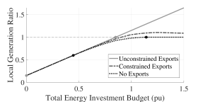
Figure 1: Comparison of relationship between maximum achievable local generation ratio, $\overline{\mathcal{X}}_{i}$, and total energy investment budget, $\sum_{t\in\mathcal{T}}\overline{P}^{\text{S}+}_{i,t}$, under different power export constraints. The total energy investment budget is given in per unit using the total energy demand, $\sum_{t\in\mathcal{T}}P^{\text{L}}_{i,t}$ , as a base.

II-C Communities with Constrained Power Exports

In practice, the ability of a given community to export excess generated power may be constrained by a number of factors including capacity limits of physical grid infrastructure (e.g., substation transformers, transmission or distribution lines), or the willingness of surrounding communities to consume that power. We model these constraints as bounds on the difference in additional power generation and demand. That is,

$$\underline{P}^{\text{S}}_{i,t}\leq P^{\text{S}+}_{i,t}-P^{\text{S}-}_{i,t}\leq\overline{P}^{\text{S}}_{i,t}\,.$$ (5)

Note that since $P^{\text{G}}_{i,t}$ and $P^{\text{L}}_{i,t}$ are treated as fixed data, constraints of the form (5) are sufficient to capture limits on net exports from community $i$.

Following the same logic as in Sec. II-B, we want to make $P^{\text{S}+}_{i,t}$ as large as possible and $P^{\text{S}-}_{i,t}$ as small as possible, in order to maximize $\mathcal{X}_{i}$. If $\overline{P}^{\text{S}}_{i,t}>=\overline{P}^{\text{S}+}_{i,t}$ for a given time $t$, then we can set $P^{\text{S}+}_{i,t}=\overline{P}^{\text{S}+}_{i,t}$ and $P^{\text{S}-}_{i,t}=0$, as we did in Sec. II-B. However, if $\overline{P}^{\text{S}}_{i,t}<\overline{P}^{\text{S}+}_{i,t}$ for a given time $t$, then the constraint (5) is binding. Therefore, we set $P^{\text{S}-}_{i,t}=P^{\text{S}+}_{i,t}-\overline{P}^{\text{S}}_{i,t}$. Under these conditions, we can maximize $\mathcal{X}_{i}$ by setting $P^{\text{S}+}_{i,t}=\overline{P}^{\text{S}+}_{i,t}$ and $P^{\text{S}-}_{i,t}=\overline{P}^{\text{S}+}_{i,t}-\overline{P}^{\text{S}}_{i,t}$, assuming $\sum_{t\in\mathcal{T}}\overline{P}^{\text{S}}_{i,t}\geq\sum_{t\in\mathcal{T}}(P^{\text{L}}_{i,t}-P^{\text{G}}_{i,t})$. Combining the two above cases ($\overline{P}^{\text{S}}_{i,t}>=\overline{P}^{\text{S}+}_{i,t}$ and $\overline{P}^{\text{S}}_{i,t}<\overline{P}^{\text{S}+}_{i,t}$), we obtain an updated expression for the maximum local generation ratio,

$$\overline{\mathcal{X}}_{i}=\frac{\sum_{t\in\mathcal{T}}(P^{\text{G}}_{i,t}+\overline{P}^{\text{S}+}_{i,t})}{\sum_{t\in\mathcal{T}}(P^{\text{L}}_{i,t}+\max\{\overline{P}^{\text{S}+}_{i,t}-\overline{P}^{\text{S}}_{i,t}\,,0\})}\,,$$ (6)

which accounts for a community’s power export constraints.

Examples of the relationship between $\overline{\mathcal{X}}_{i}$ and total energy investment budget for different power export constraints are shown in Fig. 1. Note that until a certain point, all curves in Fig. 1 follow the same line as the unconstrained case. However, once a community’s ability to export excess generation is constrained at some time $t$, it will begin to require larger investments in order to achieve the same value of $\mathcal{X}_{i}$ as the unconstrained case.

Fig. 1 also shows the special case where a community is unable to export any excess power. In order to achieve a value of $\mathcal{X}_{i}=1$ in this case, the community will need to invest in enough local generation assets to completely meet its local demand at all times (i.e., the community will need to operate as a microgrid).

II-D Equity Considerations in Energyshed Planning

It is important to recognize that different communities will have different capabilities to invest in new energy assets. Unless careful consideration is given to the diversity in resources that is inherent to different communities, some frameworks for energyshed planning can lead to inequitable outcomes for some communities.

For example, communities with the capability (more resources, larger budget) to invest in local generation resources the fastest will be able to achieve values of $\mathcal{X}_{i}\geq 1$ more quickly by exporting excess generation to less-privileged communities. However, if each community makes independent decisions with the goal of maximizing its own $\mathcal{X}_{i}$, then as the least privileged communities invest in local generation resources, they may not have the opportunity to export excess power (since importing power would decrease $\mathcal{X}_{i}$ for surrounding communities). Thus, communities which are the slowest to achieve their energyshed policy goals will have to invest disproportionately more resources to meet those goals. This motivates the need for a cooperative energyshed planning framework, where the impact of decisions made by one community on neighboring communities is considered explicitly, in order to achieve better system-wide outcomes.

III Cooperative Energyshed Planning Framework

In this section, we propose an optimization-based, cooperative framework for energyshed planning and decision-making. We denote the set of nodes in the network that operate as energysheds by $\mathcal{N}_{ES}\subseteq\mathcal{N}$. The energyshed planning problem can then be formulated as follows:

$$\max_{P_{i,t}^{\text{S}+},P_{i,t}^{\text{S}-}}~{}~{} \min_{i}(\mathcal{X}_{i})-\alpha\sum_{(i,j)\in\mathcal{E}}(\sum_{t\in\mathcal{T}}|{P_{ij,t}}|)\,,$$ (7a)

s.t. $$P_{i,t}^{\text{G}}-P_{i,t}^{\text{L}}+P_{i,t}^{\text{S}}=\sum_{j:(i,j)\in\mathcal{E}}P_{ij,t}\,,~{}\forall i\in\mathcal{N}\,,~{}\forall t\in\mathcal{T}\,,$$ (7b)

$$P_{ij,t}=\frac{\theta_{i,t}-\theta_{j,t}}{x_{ij}}\,,~{}\theta_{1,t}=0\,,~{}\forall(i,j)\in\mathcal{E}\,,~{}\forall t\in\mathcal{T}\,,$$ (7c)

$$P_{i,t}^{\text{S}}=P_{i,t}^{\text{S}+}-P_{i,t}^{\text{S}-}\,,~{}\forall i\in\mathcal{N}\,,~{}\forall t\in\mathcal{T}\,,$$ (7d)

$$\mathcal{X}_{i}=\frac{\sum_{t\in\mathcal{T}}(P^{\text{G}}_{i,t}+P^{\text{S}+}_{i,t})}{\sum_{t\in\mathcal{T}}(P^{\text{L}}_{i,t}+P^{\text{S}-}_{i,t})}\,,~{}~{}\forall i\in\mathcal{N}_{ES}\,,$$ (7e)

$$0\leq P_{i,t}^{\text{S}+}\leq\overline{P}_{i,t}^{\text{S}+}\,,~{}~{}\forall i\in\mathcal{N}\,,~{}~{}\forall t\in\mathcal{T}\,,$$ (7f)

$$0\leq P_{i,t}^{\text{S}-}\leq\overline{P}_{i,t}^{\text{S}-}\,,~{}~{}\forall i\in\mathcal{N}\,,~{}~{}\forall t\in\mathcal{T}\,,$$ (7g)

$$\underline{P}_{ij,t}\leq P_{ij,t}\leq\overline{P}_{ij,t}\,,~{}\forall(i,j)\in\mathcal{E}\,,~{}\forall t\in\mathcal{T}\,.$$ (7h)

The objective function (7a) consists of two terms. The goal of the first term is to maximize the minimum value of $\mathcal{X}_{i}$ across all energysheds. This incentivizes communities to cooperate in supporting the energyshed with the smallest local generation ratio achieve their policy goals. The solution of the optimization problem (7) is non-unique, since $\mathcal{X}_{i}$ variables that are not the minimum can take multiple values at optimality. By adding the second term of (7a), we attempt to reduce the number of non-unique solutions. This term penalizes the power flows, $P_{ij,t}$, in each line $(i,j)$ of the network and each time $t$. Furthermore, by selecting a large value for the weight $\alpha$, we can study scenarios where sharing power between communities is discouraged.

The constraints (7b)–(7c) represent the DC power flow equations for the network at each time $t$, where $x_{ij}$ is the line reactances and $\theta_{i,t}$ is the voltage phase angle (in radians) of node $i$. The definitions of $P^{\text{S}}_{i,t}$ and $\mathcal{X}_{i}$ are captured by (7d)–(7e), whereas constraints (7f)–(7g) enforce investment budgets. Finally, line flow limits are given by (7h), respectively. Note that the constraint (7e) is non-convex. Thus, in this paper, we utilize nonlinear programming (NLP) techniques, such as interior-point methods, to solve (7).

IV Numerical Case Study

In order to study the fundamental tradeoffs associated with energyshed policy decisions within power systems, we tested the proposed cooperative planning framework on the 6-bus transmission network shown in Fig. 2(a) [11]. The cooperative planning framework is implemented in Julia using the JuMP package [12], and the NLP (7) is solved with the Ipopt solver [13]. We consider the set $\mathcal{T}$ as every hour over the course of one day. Unless otherwise noted, per unit quantities are provided on a 100 MVA system base.

Figure 2: Six-bus transmission test network [11]. (a) One-line diagram. (b) Load and existing distributed generation profiles for Buses 4–6.

Buses 1, 2, and 3 have no local load and are equipped with conventional synchronous generation. Therefore, we do not treat them as energysheds or consider values of $\mathcal{X}_{i}$ for these buses. Within the energyshed planning framework, we determine the power dispatch for these conventional generating units through the variable $P^{\text{S}}_{i,t}$ (rather than $P^{\text{G}}_{i,t}$). For all times $t$, $\overline{P}^{\text{S}+}_{i,t}$ is set to the maximum power limit for each generator (2.0, 1.5, and 1.8 pu on Buses 1, 2, and 3, respectively), and $\overline{P}^{\text{S}-}_{i,t}$ is zero. We assume Buses 4, 5, and 6 all operate as energysheds. The load and existing distributed generation profiles for these buses over the day are shown in Fig. 2(b). Line flow limits for each transmission line, with $\underline{P}_{ij,t}=-\overline{P}_{ij,t}$, are identical to those in the MATPOWER case data for the 6-bus system [11], with the exception that line limits for Lines 3–6, 1–4, and 2–4 are increased to 1.0, 0.8, and 0.8 pu, respectively, in order to alleviate infeasibility issues due to transmission constraints.

In the following case study, we vary the total energy investment budget, $\sum_{t\in\mathcal{T}}\overline{P}^{\text{S}+}_{i,t}$, and investigate the tradeoffs of energyshed planning decisions under different power sharing scenarios (i.e., values of the weight $\alpha$). To account for the diversity of resources that is inherent to different communities, we assume that for each unit of additional investment budget in Bus 4, Buses 5 and 6 are able to increase their investment budgets by 1.5 units and 3 units, respectively. That is, if we choose a budget $\overline{P}\in[0,1.5]$ pu, then the budgets for Buses 4–6 are $\overline{P}^{\text{S}+}_{i,t}=\{\overline{P},~{}1.5\,\,\overline{P},~{}3.0\,\,\overline{P}\}$ for all times $t$. For simplicity, we assume $\overline{P}^{\text{S}+}_{i,t}$ is constant with respect to time, and set $\overline{P}^{\text{S}-}_{i,t}=\overline{P}^{\text{S}+}_{i,t}$.

Fig. 3 shows the values of $\mathcal{X}_{i}$ at Buses 4–6 as the total energy investment budget is increased, under a more cooperative planning framework ($\alpha=0.001$) and a scenario where sharing power between communities is discouraged ($\alpha=0.1$). In the $\alpha=0.1$ case, the energysheds at Buses 5 and 6 (which have more available resources) are able to achieve values of $\mathcal{X}_{i}\geq 1$ quickly. However, once these communities reach their policy goals, they are no longer willing to import excess generation from Bus 4. Thus, the energyshed at Bus 4 (i.e., the least privileged community) requires much more investment in energy assets to reach $\mathcal{X}_{i}=1$. In contrast, with $\alpha=0.001$, the energysheds at Buses 5 and 6 import excess generation from Bus 4 (even if that means achieving their own policy goals at a slower pace, or even slightly reducing their value of $\mathcal{X}_{i}$), in order to allow the energyshed at Bus 4 to follow the linear trajectory (i.e. corresponding to unconstrained exports) for much longer. This results in Bus 4 being able to achieve 100% local energy generation ($\mathcal{X}_{i}=1$) with approximately 28% less investment burden.

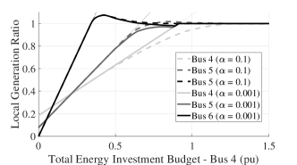
Figure 3: Comparison of local generation ratio at Buses 4–6, as a function of total energy investment, for different degrees of power sharing penalization. The total energy investment for Buses 5 and 6 are plotted in terms of total energy investment in Bus 4.

Finally, Fig. 4 illustrates the tradeoffs between the minimum $\mathcal{X}_{i}$ (i.e., the first term of the objective function), network utilization (the second term of the objective), and the total energy dispatch of conventional “centralized” generation as communities invest in local generation resources. It can be seen that as communities pursue energyshed policy goals by investing in local energy assets, existing transmission and conventional generation infrastructure will be under-utilized and may become sunk costs. Furthermore, while this work intentionally tried to remain technology and cost agnostic, it is important to recognize that investments in local energy assets will have economic, environmental, and social benefits and costs. Therefore, future research in energyshed planning that considers these aspects will be of upmost value. For example, the development of tools and processes that support communities in allocating appropriate technology and investments to meet their net generation profile $P^{\text{S}}_{i,t}$ (as determined by the proposed cooperative planning framework), is of particular interest.

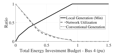
Figure 4: Comparison of local generation ratio, network utilization, and conventional generation as communities increase investments in local energy assets.

V Conclusion

In this paper, we proposed a mathematical definition for energysheds, and studied the fundamental tradeoffs associated with energyshed policy decisions and planning within an electric power system. We also explored how interactions between planning decisions across different communities can potentially lead to inequitable outcomes, and introduced a framework for cooperative energyshed planning. Theoretical insights into energyshed thinking as well as a numerical case study were also presented.

There are numerous potential avenues for future research in energyshed planning. First, the proposed framework could be extended to consider AC network analysis (i.e., system voltages, reactive power flows, and line losses) or multi-energy systems (e.g., district heating or transportation systems), rather than only considering electric infrastructure. Future work could also investigate how investments in energy efficiency can be explicitly modeled in an energyshed planning framework. Additionally, further analysis into convex reformulations or relaxations of the proposed optimization problem would enable improvements in scalability to larger systems. Finally, the application of the proposed framework to large regions with real data, and consideration of economic, environmental, and social aspects of community energy planning and investment would be extremely valuable.

VI Acknowledgement

The authors greatly appreciate numerous team discussions about energysheds with colleagues at UVM, including Jeff Marshall, Jon Erickson, Greg Rowangould, Dana Rowangould, Bindu Panikkar, Hamid Ossareh, Eric Seegerstrom, Emmanuel Badmus, and Omid Mokhtari, as well as utility partners at Green Mountain Power (GMP), Vermont Electric Cooperative (VEC), Stowe Electric Department, and Vermont Electric Company (VELCO).

References

- [1] “Bringing infrastructure home,” Rewiring America, Washington D.C., USA, Tech. Rep., Jun. 2021.
- [2] A. De La Garza, “This Vermont utility is revolutionizing its power grid to fight climate change. Will the rest of the country follow suit?” Time Magazine, Jul. 2021.
- [3] U.S. Department of Energy Office of Energy Efficiency & Renewable Energy, “Clean energy to communities program,” energy.gov, Accessed: Nov. 18, 2023. [Online.] Available: https://www.energy.gov/eere/clean-energy-communities-program.
- [4] L. Illing, K. Yee, and R. Knapp, “From watershed to energyshed: Determining the implications of place-based power generation workshop and request for information summary report,” U.S. Department of Energy Office of Energy Efficiency & Renewable Energy, Washington D.C., USA, Tech. Rep., 2022.
- [5] J. C. Evarts, “Energyshed framework: Defining and designing the fundamental land unit of renewable energy,” Master’s thesis, Dalhousie University, Halifax, Nova Scotia, April 2016.
- [6] C. DeRolph et al., “City energysheds and renewable energy in the United States,” Nature Sustainability, no. 2, pp. 412–420, 2019.
- [7] A. Thomas and J. D. Erickson, “Rethinking the geography of energy transitions: Low carbon energy pathways through energyshed design,” Energy Research & Social Science, vol. 74, p. 101941, 2021.
- [8] K. Schreiber et al., “Quantifying the foodshed: a systematic review of urban food flow and local food self-sufficiency research,” Environmental Research Letters, vol. 16, no. 2, p. 023003, 2021.
- [9] “2022 Vermont comprehensive energy plan,” Vermont Department of Public Service, Montpelier, VT, Tech. Rep., 2022.
- [10] S. Chevalier and M. R. Almassalkhi, “Towards optimal Kron-based reduction of networks (Opti-KRON) for the electric power grid,” in IEEE CDC, Cancún, Mexico, 2022, pp. 5713–5718.
- [11] R. Zimmerman et al., “Matpower: Steady-state operations, planning, and analysis tools for power systems research and education,” IEEE Trans. Power Syst., vol. 26, no. 1, pp. 12–19, 2011.
- [12] M. Lubin et al., “JuMP 1.0: Recent improvements to a modeling language for mathematical optimization,” Math. Program. Computation, 2023.
- [13] A. Wächter and L. Biegler, “On the implementation of a primal-dual interior point filter line search algorithm for large-scale nonlinear programming,” Math. Program., vol. 106, no. 1, pp. 25–57, 2006.