Koopman Learning with Episodic Memory

Abstract

Koopman operator theory, a data-driven dynamical systems framework, has found significant success in learning models from complex, real-world data sets, enabling state-of-the-art prediction and control. The greater interpretability and lower computational costs of these models, compared to traditional machine learning methodologies, make Koopman learning an especially appealing approach. Despite this, little work has been performed on endowing Koopman learning with the ability to learn from its own mistakes. To address this, we equip Koopman methods – developed for predicting non-stationary time-series – with an episodic memory mechanism, enabling global recall of (or attention to) periods in time where similar dynamics previously occurred. We find that a basic implementation of Koopman learning with episodic memory leads to significant improvements in prediction on synthetic and real-world data. Our framework has considerable potential for expansion, allowing for future advances, and opens exciting new directions for Koopman learning.

1 Introduction

Over the past decade, Koopman learning [1] has emerged as a leading framework for modeling real-world dynamical systems. The development of numerical methods to efficiently approximate spectral objects associated with the Koopman operator from data [2, 3, 4, 5, 6] has led to high quality forecasting of complex time-series, such as Earth’s magnetic field [7], highway traffic patterns [8], climate indicators [9], and COVID-19 spreading [10]. The generalization of Koopman operator theory to include controlled dynamical systems [11, 12, 13, 14] has led to state-of-the-art control of soft robotics [15, 16, 17, 18]. And the advancement of theoretical results [19, 20, 21, 4, 22], linking Koopman spectral objects to state-space geometry – as well as the inherent linearity of the Koopman operator – has enabled the interpretation of learned models to an unprecedented degree.

Unlike many traditional machine learning (ML) methods, such as convolutional neural networks, that are trained to extract informative features of the data (i.e., observable functions), Koopman learning identifies dynamical relationships between observables. Thus, while requiring appropriate observables to be chosen by a knowledgeable human or ML [23, 5, 24, 25], Koopman learning can easily discover spatio-temporal interactions that are crucial to understanding the behavior of the system under study.

Koopman learning’s data-driven, predictive, efficient, controllable, interpretable, and dynamics-based properties make it well aligned with next generation artificial intelligence. And yet, to-date, there has been almost no work on enabling Koopman learning to learn from its previous mistakes, an essential aspect of any “intelligent” framework. The need for such an approach becomes clear when considering applying Koopman learning to non-autonomous dynamical systems [such as the yearly flu cases in the United States (U.S.), Fig. 1A], where temporally local Koopman models are generated over streaming or sliding time windows [26, 8, 10]. While this mitigates the mixing of data from distinct dynamical regimes, its implicit forgetting of the past requires any repeated structure of the data (Fig. 1B) to be re-learned from scratch.

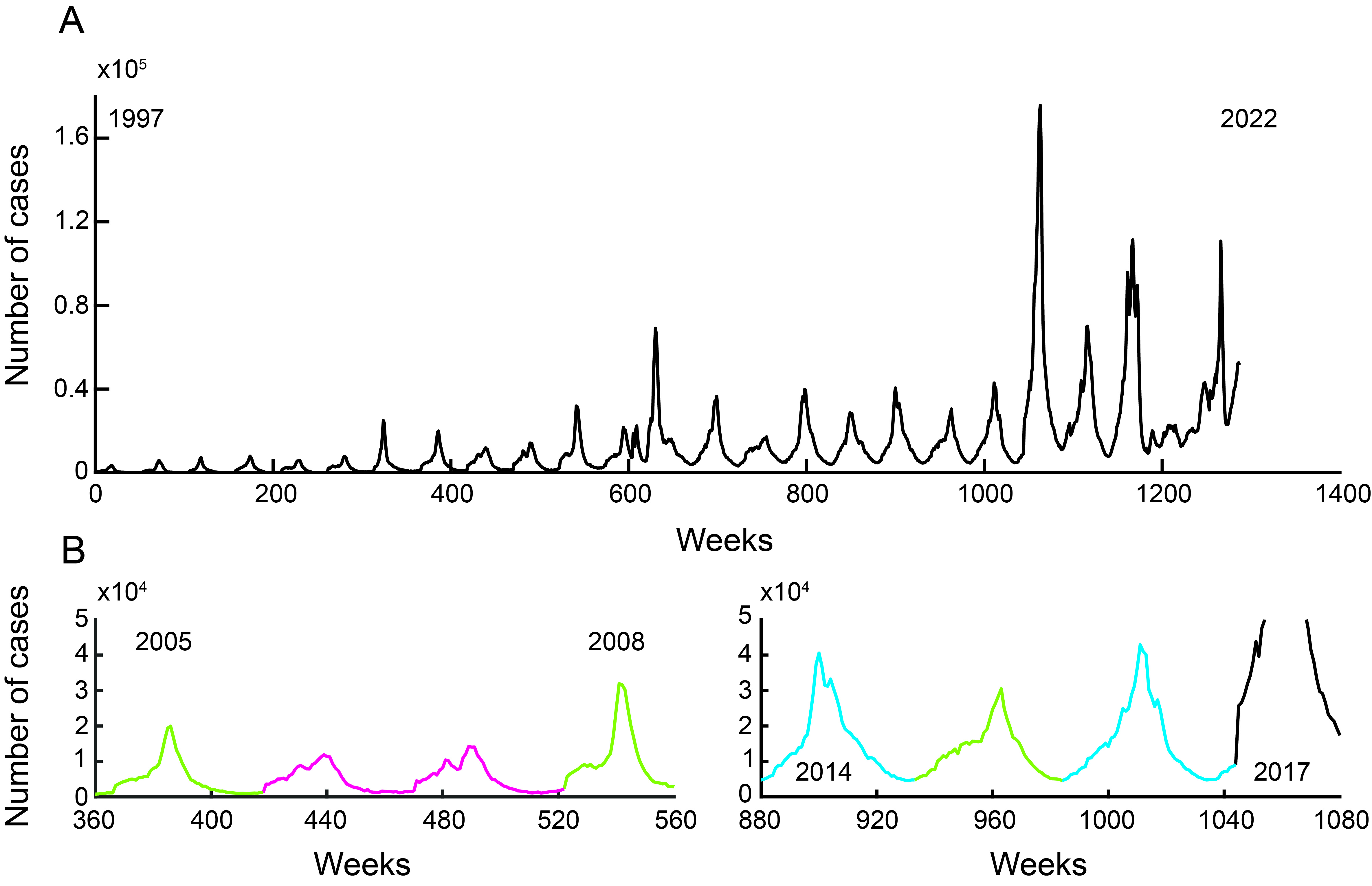
Figure 1: Example of repeated structure in non-stationary dynamical system. (A) Number of flu cases per week in the U.S. from 1997 to 2022, as reported to CDC by Public Health Laboratories. (B) Zoomed-in four year time windows of (A). Years are colored by their qualitative similarities in shape and peak amplitude.

Traditional ML methods have long wrestled with this problem, and – in their application to time-series – the use of memory has proven to be useful. This was done first by recurrent neural networks (RNNs) [27], whose within-layer connectivity enables information to remain in the network through time, affecting future internal states. The introduction of long short-term memory (LSTM) networks [28] and liquid state machines [29] led to computationally tractable models that became widely adopted. However, in these models, long histories (or “memory traces”) are continually present, making training challenging and susceptible to vanishing gradients. Over the past several years, Transformer networks [30], which make use of the self-attention mechanism – originally designed to improve upon RNNs used for machine translation [31] – have performed dominantly in a number of domains, attesting to the power selectively attending to global aspects of data can confer. In the context of time-series prediction, where Transformers have become increasingly utilized [32, 33, 34, 35], self-attention can be viewed as recalling specific points in the past that are relevant to the present. Despite these advances, the high computational costs required to train such models, as well as the mixed performance gains reported when comparing Transformers to linear models [36], suggests that there may be room for improvement from alternative approaches.

Inspired by the integration of memory into traditional ML methods, we develop an approach that saves spectral objects associated with temporally local approximations of the Koopman operator, and utilizes this information to make new predictions, that are informed from the past. Because the Koopman spectral objects are computed over a time window, these compact representations of the dynamics capture episodes of previously observed data. Therefore, we refer to the general framework we introduce as Koopman learning with episodic memory (Fig. 2). Through deployment on synthetic and real-world data sets, we show that the specific realization of Koopman learning with episodic memory we develop, called extended dynamic mode decomposition (EDMD) with memory, sees large improvements in prediction accuracy. This comes in large part from the ability of these models to not repeatedly make the same mistakes. We believe that our work not only demonstrates a way in which to better applications of Koopman operator theory to the prediction of non-autonomous dynamical systems, but additionally advances the state of Koopman learning as an artificial intelligence framework, opening up a wealth of future directions.

2 Koopman operator theory

The central object of interest in Koopman operator theory is the Koopman operator, $U$, an infinite-dimensional linear operator that describes the time evolution of observables (i.e., functions of the underlying state-space variables) that live in the functional space $\mathcal{F}$ [37, 38, 19]. In particular, after $t>0$ amount of time, which can be continuous or discrete, the value of the observable $f\in\mathcal{F}$, which can be a scalar or a vector valued function, is given by

$$U^{t}f(x_{0})=f\left[T^{t}(x_{0})\right],$$ (1)

where $T$ is the dynamical map evolving the system and $x_{0}$ is the initial condition in state-space. For the remainder of the paper, it will be assumed that the state-space being considered is of finite dimension and that $\mathcal{F}$ is a suitably chosen space of functions in which the spectral expansion exists [22].

The action of the Koopman operator on the observable $f$ can be decomposed as

$$Uf(p)=\sum_{i=0}^{\infty}\lambda_{i}\phi_{i}(x_{0})v_{i},$$ (2)

where the $\phi_{i}$ are eigenfunctions of $U$, with $\lambda_{i}\in\mathbb{C}$ as their eigenvalues and $v_{i}$ as their Koopman modes [19, 22].

Spectrally decomposing the action of the Koopman operator is powerful because, for a discrete-time dynamical system, the value of $f$ at time step $k\in\mathbb{Z}^{+}$ is given simply by

$$f\left[T^{k}(x_{0})\right]=U^{k}f(x_{0})=\sum_{i=0}^{\infty}\lambda_{i}^{k}\phi_{i}(x_{0})v_{i}.$$ (3)

From Eq. 3, we see that the dynamics of the system in the directions $v_{i}$, scaled by $\phi_{i}(x_{0})$, are given by the magnitude of the corresponding $\lambda_{i}$. For the remainder of the paper, we will consider the output of the Koopman mode decomposition (KMD) being the Koopman eigenvalues, $\lambda_{i}$, and the scaled Koopman modes, $\phi_{i}(x_{0})v_{i}$, which we will refer to as “Koopman modes” for simplicity.

2.1 Extended dynamic mode decomposition

There exist many ways of numerically approximating the KMD from a data matrix $X=[x_{0},x_{1},...,x_{m-1}]$, where $x_{i}\in\mathbb{C}^{n}$ are snapshots of the underlying dynamical system. In the case that a single observable (i.e., $n=1$) is recorded from the system under study, time delays can be introduced, so as to enlarge the set of observables [39]. A popular approach to compute the KMD is dynamic mode decomposition (DMD) [40, 2]. DMD aims to find a matrix $A\in\mathbb{C}^{n\times n}$, such that

$$||AX-Y||_{F},$$ (4)

is minimized with respect to the Frobenius norm, where $Y=[x_{1},...,x_{m}]$. A solution to Eq. 4 is given by

$$A=YX^{+},$$ (5)

where $+$ is the Moore-Penrose pseudo-inverse [2, 40, 41]. Practically, $A$ is often approximated by performing reduced singular value decomposition (SVD) [40, 41]. While simple, this approach yields the KMD when certain conditions are met [2]. These conditions are restrictive, and in general, are not guaranteed to be satisfied. In addition, it is often the case that the action of the Koopman operator, restricted to the identity observable (that is, the original state-space variables), is not invariant. For these, and other reasons, many variants to DMD have been proposed.

One such approach is extended dynamic mode decomposition (EDMD) [3], which considers not the data matrices $X$ and $Y$, but a dictionary of functions $\mathcal{D}=[\psi_{1},...,\psi_{k}]$ applied to $X$ and $Y$. That is, it considers the functions $\Psi(x)=[\psi_{1}(x),...,\psi_{k}(x)]$, where $\Psi:\mathbb{C}^{n}\rightarrow\mathbb{C}^{k}$. The Koopman operator is then approximated as

$$K=G^{+}A,$$ (6)

where

$$\centering G=\frac{1}{m}\sum_{i=1}^{m}[\Psi(x_{i})]^{*}\Psi(x_{i})\hskip 28.45274ptA=\frac{1}{m}\sum_{i=1}^{m}[\Psi(x_{i})]^{*}\Psi(y_{i}).\@add@centering$$

EDMD introduces a choice of which set of functions to include in the dictionary $\mathcal{D}$, which can be addressed from an understanding of the nature of the data [42], as well as can be optimized via dictionary learning [23]. In this paper, we consider a family of Gaussian radial basis functions as the dictionary, but our approach generalizes beyond this decision.

3 Koopman learning with episodic memory

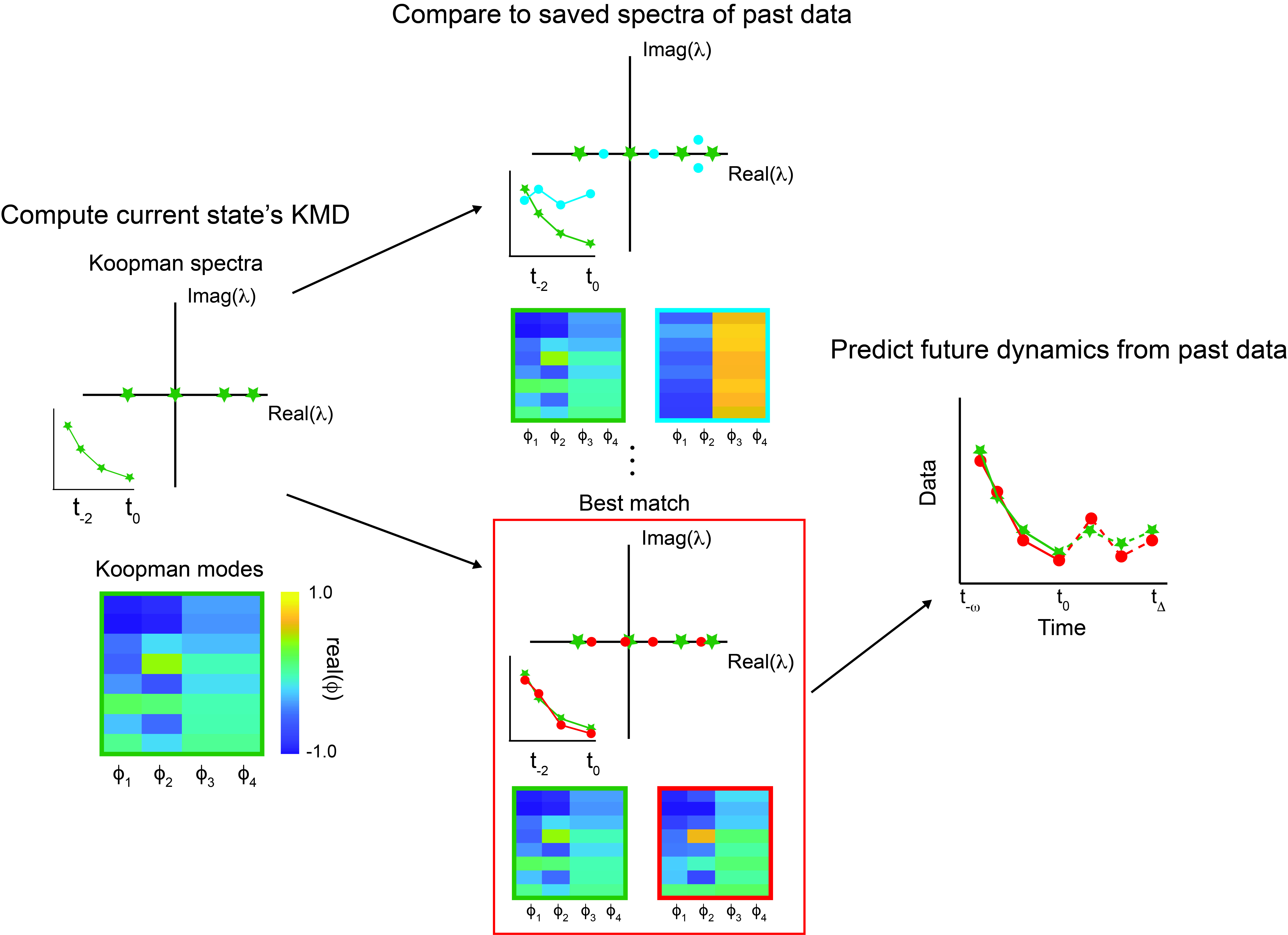
Figure 2: Overview of episodic memory for Koopman learning. For the current state of the system under study, the data within the sliding window (inset figure on left) is used to compute the KMD. The resulting Koopman spectra and modes are then compared to a library (or memory bank) of saved Koopman spectra and modes, associated with past data. If a match of both Koopman spectra and modes is found (illustrated by the red box), then the data that occurred in the past (dashed red line) is used to predict the future behavior of the system (dashed green line). If no match is found, sliding EDMD is used to generate a prediction.

A motivation for the integration of episodic memory in Koopman learning is the existence of repeated structure in some non-stationary dynamical systems (Fig. 1B). These patterns can emerge when underlying interactions between components of the system are constant (e.g., human contact patterns), as well as when constraints of the system are constant (e.g., healthcare infrastructure and supply chains).

In order to identify when data currently being observed has similar dynamical features to data seen in the past, three ingredients are necessary. First, a representation of the dynamical features of data is needed. Given that Koopman operator theory decomposes data into Koopman eigenvalues and modes (Eq. 2), the compact representation of the KMD satisfies this requirement. In this paper, we use EDMD [3] (Eq. 6) to approximate the Koopman spectral objects, but our approach applies broadly to other numerical methods [6]. Second, a way to compare dynamical features is needed, so that the notion of “similarity” can be quantified. Previous work comparing the Koopman spectra across dynamical systems [43, 44] has used the Wasserstein distance, a metric from optimal transport that measures how much one distribution has to be modified to match another. We use the same approach here, although again, other choices could be made. Finally, the dynamical features need to be saved for future comparison. Here, we simply store the Koopman spectra and modes, associated with all local time windows, in very basic data structures. Future applications of this approach can make use of more sophisticated ways in which to efficiently save the Koopman representations, as well as ways in which to incorporate the current KMD with similar saved representations (see Discussion).

3.1 Algorithm

Our implementation of Koopman learning with episodic memory (EDMD with memory), on a data set $X=[x_{0},...,x_{T}]$, has four primary steps:

1) At time step $t$, EDMD is performed on the window of data $\left[x_{t},...,x_{t+\omega}\right]$, where $\omega\in\mathbb{Z}^{+}$ is the size of the sliding window. We refer to this approach as “sliding EDMD”.

2) The computed Koopman eigenvalues and modes are compared to the Koopman eigenvalues and modes saved from all previous time windows, via the Wasserstein distance.

3) The time window $[t_{\text{min}}-\omega,t_{\text{min}}]$, whose Koopman eigenvalues and modes have the smallest Wasserstein distance with the current Koopman eigenvalues and modes, is identified. If the Wasserstein distance is smaller than a pre-determined threshold, $\varepsilon\in\mathbb{R}^{+}$, we predict $\Delta$ steps into the future by directly using what previously occurred after $t_{\text{min}}$. That is, we set $\hat{x}_{t+\Delta}=x_{t_{\text{min}}+\Delta}$, where $\hat{x}_{t+\Delta}$ is the prediction and $x_{t_{\text{min}}+\Delta}$ is the value of the data that occurred after the previous time window with similar dynamics. In this way, EDMD with memory “remembers” what happened last time similar dynamics occurred. If the closest saved spectral objects have Wasserstein distance greater than $\varepsilon$, then the standard sliding EDMD prediction is used. In practice, different values of $\varepsilon$ can be defined for the Koopman eigenvalues and modes ($\varepsilon_{\lambda}$ and $\varepsilon_{\text{mode}}$, respectively).

4) After prediction, the computed Koopman eigenvalues and modes from the current time window are stored with all the other previously saved spectral objects.

Note that in our current implementation, we only allow information from one memory to be used, and for the prediction to be exactly what occurred before (up to scaling, see below). Combining information across multiple similar memories is an exciting direction that we will pursue in future work.

4 Results

4.1 Synthetic piecewise exponential data

To probe the predictive capabilities of EDMD with memory, we first designed a synthetic data set that standard sliding EDMD performed poorly on. Namely, we generated data coming from a piecewise exponential dynamical system described by

$$x_{t}=\lambda_{t}x_{t-1}(1+\eta\xi),$$ (7)

where $\lambda_{t}\in\{-1.0101,-0.99,0.99,1.0101\}$ and is pseudo-randomly re-sampled every $10$ time steps, and $\xi$ is a random variable drawn from a stationary Gaussian distribution of mean $0$ and variance $1$, with $\eta$ acting as a magnitude of the noise.

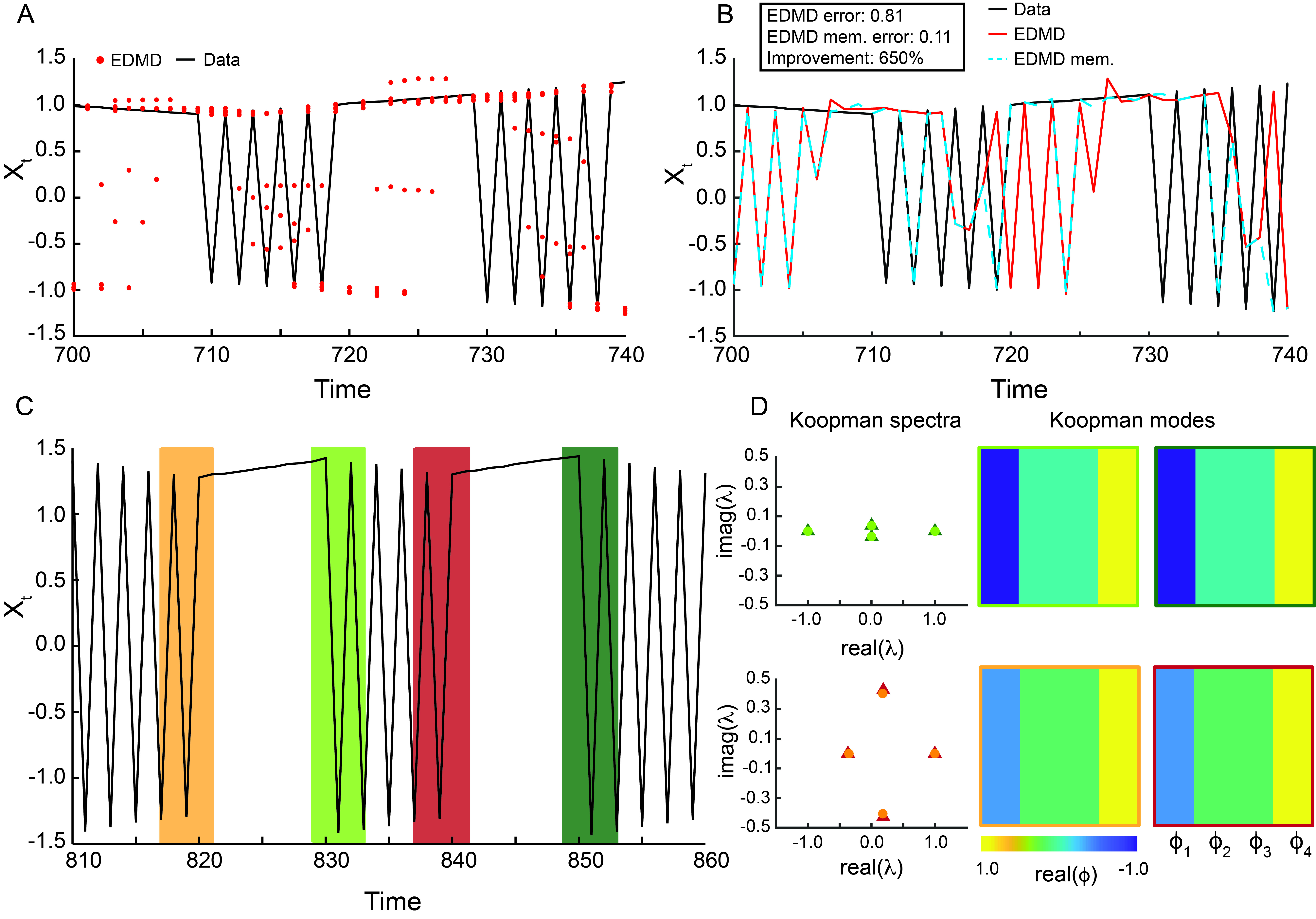
Figure 3: Episodic memory improves the ability of Koopman learning to predict synthetic non-stationary exponential data. (A) The predictions of sliding EDMD $\Delta=1,...,5$ time steps (red dots), often poorly match the true data. (B) Utilizing EDMD memory (blue line) leads to $650\%$ improvement on predictions, as compared to sliding EDMD (red line). Note that while a zoomed-in section is shown here, the improvement was computed over a $1000$ time-step simulation. (C) Because there are a finite (and small) number of possible values $\lambda_{t}$ can take, there is repetition of transitions (examples highlighted in green and orange) rectangles. (D) These repetitions can be identified by characteristic Koopman spectral objects [colored the same as in (C)].

As can be seen, the predictions from sliding EDMD does a poor job matching the true evolution of $x_{t}$ when the sliding window includes data from two different values of $\lambda_{t}$ (Fig. 3A, B). However, while the Koopman models from these windows having information that is not directly helpful for prediction, they do have identifiable Koopman eigenvalues and modes across repeats of the same transitions (e.g., $\lambda_{t}=-0.99\rightarrow\lambda_{t}=1.0101$) (Fig. 3C, D). This suggests that utilizing the episodic memory mechanism may lead to improvements in prediction.

Because $x_{t}$ can grow and shrink with time (depending on whether $|\lambda_{t}|>1$ or $|\lambda_{t}|<1$), time windows with matching dynamics (and thus, similar Koopman eigenvalues and modes) can have different magnitudes of $x_{t}$. This can complicate directly using previously observed data as predictions. We correct for this by computing the ratio between the current time point’s magnitude and that of the first time point in the recalled time window, and using this ratio as a re-scaling factor for our prediction. Additionally, we adaptively set the variance of the Gaussian radial basis dictionary functions to be the maximum value in the current sliding window, instead of the maximum value over the entire data set. This helps mitigate slight differences in Koopman spectra that artificially arise due to differences in scale.

We find that the episodic memory mechanism can indeed boost the predictive capability of sliding EDMD on this data set (Fig. 3B). While not perfect, EDMD with memory is more capable at accurately predicting the future state of $x_{t}$, even when the data in its sliding window comes from two different dynamical regimes (for instance, it can predict periods of oscillation, $\Delta=5$ time steps ahead, from a sliding window that includes both exponentially growing and oscillating data). This suggests that the episodic memory mechanism is mitigating the repetition of the same mistakes, once a given transition has been observed. To quantify the improvement, we compute the median relative prediction error as $100\%\times\left[\frac{\text{median}_{t}(|x_{t+\Delta}-\hat{x}_{t+\Delta}^{\text{EDMD}}|)}{\text{median}_{t}(|x_{t+\Delta}-\hat{x}_{t+\Delta}^{\text{mem}}|)}-1\right]$, where $\hat{x}_{t+\Delta}^{\text{EDMD}}$ is sliding EDMD’s prediction $\Delta$ time steps ahead at time $t$, $\hat{x}_{t+\Delta}^{\text{mem}}$ is EDMD with memory’s prediction $\Delta$ time steps at time $t$, and $\text{median}_{t}(\cdot)$ is the median value taken over all values of time. We find that EDMD with memory leads to an improvement of $650\%$ in median relative prediction error, as compared to sliding EDMD (Fig. 3B).

4.2 U.S. Flu Cases

We now turn our attention to applying EDMD with episodic memory on real-world, non-stationary data. As already mentioned in the Introduction, the number of U.S. flu cases per week has repeated structure (Fig. 1) that our episodic memory mechanism should be able to take advantage of.

We find that adding the episodic memory mechanism to sliding EDMD yields an improvement of almost $55\%$ on one-week ahead forecasting (Fig. 4A), decreasing the median relative error from $22.6\%$ to $14.6\%$. Examples of EDMD with memory’s predictions of individual yearly peaks (Fig. 4C) show clearly better matching with the ground truth. Increasing the forecast horizon to 5 weeks ahead, we again find that EDMD with memory can lead to large improvements over sliding EDMD (Fig. 4B, D), decreasing the error by over $28\%$.

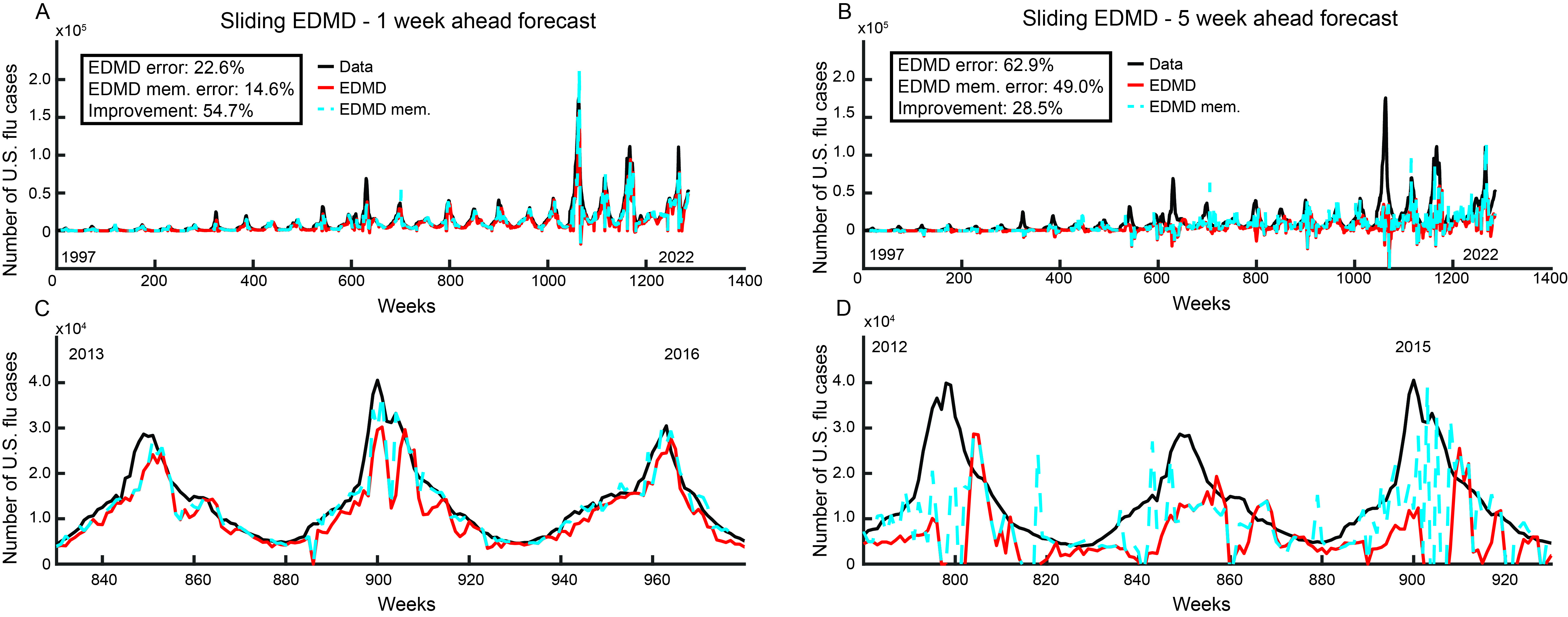
Figure 4: Episodic memory improves the ability of Koopman learning to predict the number of U.S. flu cases. (A)–(B) Predicted weekly number of U.S. flu cases one and five weeks ahead, using sliding EDMD with (blue line) and without (red line) episodic memory. Black line denotes true data. (C)–(D) Zoomed-in windows of (A) and (B).

4.3 Washington D.C. Bike Share

Lastly, we apply EDMD with memory to predict the number of bikes in use, per hour, from the Washington D.C. bike share program during January 1, 2011 – December 31, 2012 . This data set is especially challenging, given that it contains $17,000+$ time points and exhibits highly transient dynamics (Fig. 5A, B).

We find that EDMD with memory can provide improvements in median relative prediction error of more than $110\%$ over sliding EDMD, in the case of one hour ahead forecasting, and over $62\%$, in the case of four hour ahead forecasting (Fig. 5). We believe this improvement in performance, relative to the U.S. flu cases, comes from the bike share data having considerably more time points. This enables the episodic memory mechanism to learn and leverage more repeated patterns. Additionally, the variability in the data makes the application of sliding EDMD more challenging, allowing information “recalled” from the past, via the episodic memory mechanism, to have a larger impact.

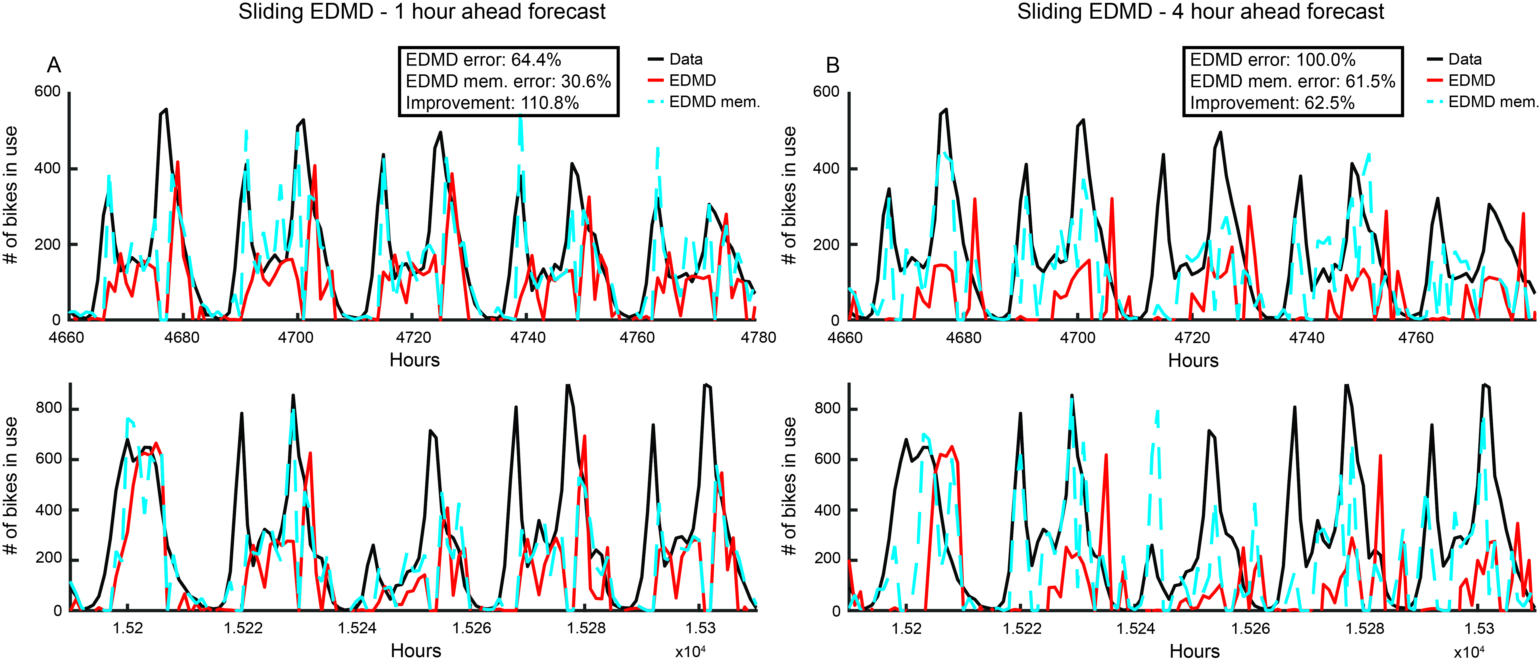
Figure 5: Episodic memory improves the ability of Koopman learning to predict the number of bikes in use, per hour, from the Washington D.C. bike share program. (A) Predicted number of bikes used one hour ahead, from the Washington D.C. bike share program using sliding EDMD with (blue line) and without (red line) episodic memory. Due to the large number of time points ($17,000+$), the data has been zoomed-in around distinct five day (120 hour) periods (top and bottom). Note that the statistics presented in the top box is computed across the entirety of the data set. (B) Same as (A), but for four hour ahead predictions.

5 Discussion

In this paper, we present an episodic memory mechanism that can be easily integrated into the framework of Koopman learning (Fig. 2) and can improve the predictive capabilities of sliding EDMD on non-stationary data (Figs. 3–5) by enabling the “recall” of what occurred directly after episodes in the past that had similar dynamical features. A simple consequence of this is that EDMD with memory is better able to learn that transient increases are followed by transient decreases in real-world data (Figs. 4 and 5). While our simple implementation of Koopman learning with episodic memory (which we call “EDMD with memory”) has limitations, it opens up a number of directions for expanding the ideas developed here that we believe will push forward the state of Koopman learning.

5.1 Limitations

While the presence of repeating structure in time-series data (e.g., Fig. 1B) motivates the development of approaches that can identify and leverage them for future prediction, the success of such methods are necessarily limited in several ways.

First, the repeated structure that EDMD with memory identifies is related to constraints and response properties of the system under study. For instance, in the case of U.S. weekly flu cases, the repeated structure is related healthcare infrastructure and supply chains, weather, and flu variants. When these are relatively consistent over the span of several years, EDMD with memory can be used to identify past data that is directly relevant. However, in the case where healthcare infrastructure and supply chains, as well as disease variants, rapidly evolve with time (as in the case of COVID-19), we expect EDMD with memory to be less useful.

A second limitation has to do with the fact that EDMD with memory requires having seen a given dynamical feature in the past to predict it. While it can, in principle, learn the pattern in a single shot (making it considerably more efficient than some standard ML methods), during the first exposure it does not contribute to the prediction. Because sliding EDMD has been found to be a powerful tool for data-driven prediction [8, 10], this should not be severely limiting to the predictive capability of our approach. However, there may be other methods, such as physics (or domain) informed techniques, that would be better to deploy in the case where first identification is critical. However, we note that the absence of a good match between the current set of spectral objects and the library of saved spectral objects, provides information. Namely, that a new regime, unlike what has been seen previously, is being entered. If the library is created from a sufficiently large set of time points, this could provide confidence that novel dynamics are being encountered, and appropriate measures could be taken.

Finally, in our current implementation of EDMD with memory, all saved Koopman eigenvalues and modes are given equal weighting, and only one, of possibly several close (with respect to the Wasserstein distance) previously saved memories, are used for prediction. Because this approach does not take into account whether this past data is close in time to the current data and/or whether this estimate came from data with high noise or uncertainty, we imagine that this approach is sub-optimal and can be improved upon.

5.2 Expansions

There are several ways in which this preliminary development of Koopman learning with episodic memory can be expanded. First, recent developments in Koopman operator theory for reduced order modeling allows for the noisy components of the Koopman spectra to be removed and the uncertainty in the estimate to be quantified [45]. Integrating this into EDMD with memory will enable better estimates of the true Koopman spectra, as well as better matching between saved spectral objects. Second, a powerful capability of Koopman operator theory is its natural connection to observables beyond the state-space variables. As many state-space variables of interest (e.g., flu cases) are naturally functions of other variables (e.g., weather), these additional observables can be added to better approximate the dynamics, in ways that existing predictive methods may struggle with. We imagine including more observables into estimates of the Koopman operator will make EDMD with memory more accurate. Finally, we believe that research into human memory and decision making [46] can be connected with our work and used to inspire further advances in Koopman learning.

Acknowledgements

We thank the members of AIMdyn Inc. for useful discussion on our results and Thomas Redman for pointing out [46]. This material is based upon work supported by the DARPA Small Business Innovation Research Program (SBIR) Program Office under Contract No. W31P4Q-21-C-0007 to AIMdyn, Inc. Any opinions, findings and conclusions or recommendations expressed in this material are those of the authors and do not necessarily reflect the views of the DARPA SBIR Program Office. Distribution Statement A: Approved for Public Release, Distribution Unlimited.

References

- [1] Igor Mezić. Koopman operator, geometry, and learning of dynamical systems. Not. Am. Math. Soc, 68(7):1087–1105, 2021.
- [2] Clarence W Rowley, Igor Mezić, Shervin Bagheri, Philipp Schlatter, and Dan S Henningson. Spectral analysis of nonlinear flows. Journal of fluid mechanics, 641:115–127, 2009.
- [3] Matthew O. Williams, Ioannis G. Kevrekidis, and Clarence W. Rowley. A data–driven approximation of the koopman operator: Extending dynamic mode decomposition. Journal of Nonlinear Science, 25(6):1307–1346, Dec 2015.
- [4] Hassan Arbabi and Igor Mezić. Ergodic theory, dynamic mode decomposition, and computation of spectral properties of the koopman operator. SIAM Journal on Applied Dynamical Systems, 16(4):2096–2126, 2017.
- [5] Bethany Lusch, J Nathan Kutz, and Steven L Brunton. Deep learning for universal linear embeddings of nonlinear dynamics. Nature communications, 9(1):4950, 2018.
- [6] Igor Mezić. On numerical approximations of the koopman operator. Mathematics, 10(7):1180, 2022.
- [7] Steven L Brunton, Bingni W Brunton, Joshua L Proctor, Eurika Kaiser, and J Nathan Kutz. Chaos as an intermittently forced linear system. Nature communications, 8(1):19, 2017.
- [8] Allan M Avila and I Mezić. Data-driven analysis and forecasting of highway traffic dynamics. Nature communications, 11(1):2090, 2020.
- [9] James Hogg, Maria Fonoberova, and Igor Mezić. Exponentially decaying modes and long-term prediction of sea ice concentration using koopman mode decomposition. Scientific Reports, 10(1):16313, 2020.
- [10] Igor Mezic, Zlatko Drmac, Nelida Crnjaric-Zic, Senka Macesic, Maria Fonoberova, Ryan Mohr, Allan Avila, Iva Manojlovic, and Aleksandr Andrejcuk. A koopman operator-based prediction algorithm and its application to covid-19 pandemic. arXiv preprint arXiv:2304.13601, 2023.
- [11] Joshua L Proctor, Steven L Brunton, and J Nathan Kutz. Dynamic mode decomposition with control. SIAM Journal on Applied Dynamical Systems, 15(1):142–161, 2016.
- [12] Joshua L Proctor, Steven L Brunton, and J Nathan Kutz. Generalizing koopman theory to allow for inputs and control. SIAM Journal on Applied Dynamical Systems, 17(1):909–930, 2018.
- [13] Milan Korda and Igor Mezić. Linear predictors for nonlinear dynamical systems: Koopman operator meets model predictive control. Automatica, 93:149–160, 2018.
- [14] Alexandre Mauroy, Igor Mezić, and Yoshihiko Susuki. The Koopman Operator in Systems and Control: Concepts, Methodologies, and Applications, volume 484. Springer Nature, 2020.
- [15] Daniel Bruder, Brent Gillespie, C David Remy, and Ram Vasudevan. Modeling and control of soft robots using the koopman operator and model predictive control. arXiv preprint arXiv:1902.02827, 2019.
- [16] Daniel Bruder, Xun Fu, R Brent Gillespie, C David Remy, and Ram Vasudevan. Data-driven control of soft robots using koopman operator theory. IEEE Transactions on Robotics, 37(3):948–961, 2020.
- [17] Daniel Bruder, Xun Fu, R Brent Gillespie, C David Remy, and Ram Vasudevan. Koopman-based control of a soft continuum manipulator under variable loading conditions. IEEE robotics and automation letters, 6(4):6852–6859, 2021.
- [18] David A Haggerty, Michael J Banks, Ervin Kamenar, Alan B Cao, Patrick C Curtis, Igor Mezić, and Elliot W Hawkes. Control of soft robots with inertial dynamics. Science Robotics, 8(81):eadd6864, 2023.
- [19] Igor Mezić. Spectral properties of dynamical systems, model reduction and decompositions. Nonlinear Dynamics, 41:309–325, 2005.
- [20] A. Mauroy, I. Mezić, and J. Moehlis. Isostables, isochrons, and koopman spectrum for the action–angle representation of stable fixed point dynamics. Physica D: Nonlinear Phenomena, 261:19–30, 2013.
- [21] Yueheng Lan and Igor Mezić. Linearization in the large of nonlinear systems and koopman operator spectrum. Physica D: Nonlinear Phenomena, 242(1):42–53, 2013.
- [22] Igor Mezić. Spectrum of the koopman operator, spectral expansions in functional spaces, and state-space geometry. Journal of Nonlinear Science, 30(5):2091–2145, Oct 2020.
- [23] Qianxiao Li, Felix Dietrich, Erik M Bollt, and Ioannis G Kevrekidis. Extended dynamic mode decomposition with dictionary learning: A data-driven adaptive spectral decomposition of the koopman operator. Chaos: An Interdisciplinary Journal of Nonlinear Science, 27(10):103111, 2017.
- [24] Samuel E Otto and Clarence W Rowley. Linearly recurrent autoencoder networks for learning dynamics. SIAM Journal on Applied Dynamical Systems, 18(1):558–593, 2019.
- [25] Enoch Yeung, Soumya Kundu, and Nathan Hodas. Learning deep neural network representations for koopman operators of nonlinear dynamical systems. In 2019 American Control Conference (ACC), pages 4832–4839. IEEE, 2019.
- [26] Senka Macesic, Nelida Crnjaric-Zic, and Igor Mezic. Koopman operator family spectrum for nonautonomous systems. SIAM Journal on Applied Dynamical Systems, 17(4):2478–2515, 2018.
- [27] Jeffrey L Elman. Finding structure in time. Cognitive science, 14(2):179–211, 1990.
- [28] Sepp Hochreiter and Jürgen Schmidhuber. Long short-term memory. Neural computation, 9(8):1735–1780, 1997.
- [29] Wolfgang Maass, Thomas Natschläger, and Henry Markram. Real-time computing without stable states: A new framework for neural computation based on perturbations. Neural computation, 14(11):2531–2560, 2002.
- [30] Ashish Vaswani, Noam Shazeer, Niki Parmar, Jakob Uszkoreit, Llion Jones, Aidan N Gomez, Łukasz Kaiser, and Illia Polosukhin. Attention is all you need. Advances in neural information processing systems, 30, 2017.
- [31] Dzmitry Bahdanau, Kyunghyun Cho, and Yoshua Bengio. Neural machine translation by jointly learning to align and translate. arXiv preprint arXiv:1409.0473, 2014.
- [32] Haixu Wu, Jiehui Xu, Jianmin Wang, and Mingsheng Long. Autoformer: Decomposition transformers with auto-correlation for long-term series forecasting. Advances in Neural Information Processing Systems, 34:22419–22430, 2021.
- [33] Yong Liu, Haixu Wu, Jianmin Wang, and Mingsheng Long. Non-stationary transformers: Exploring the stationarity in time series forecasting. Advances in Neural Information Processing Systems, 35:9881–9893, 2022.
- [34] Yuqi Nie, Nam H Nguyen, Phanwadee Sinthong, and Jayant Kalagnanam. A time series is worth 64 words: Long-term forecasting with transformers. arXiv preprint arXiv:2211.14730, 2022.
- [35] Yunhao Zhang and Junchi Yan. Crossformer: Transformer utilizing cross-dimension dependency for multivariate time series forecasting. In The Eleventh International Conference on Learning Representations, 2022.
- [36] Ailing Zeng, Muxi Chen, Lei Zhang, and Qiang Xu. Are transformers effective for time series forecasting? In Proceedings of the AAAI conference on artificial intelligence, volume 37, pages 11121–11128, 2023.
- [37] B. O. Koopman. Hamiltonian systems and transformation in hilbert space. Proceedings of the National Academy of Sciences, 17(5):315–318, 1931.
- [38] B. O. Koopman and J. v. Neumann. Dynamical systems of continuous spectra. Proceedings of the National Academy of Sciences, 18(3):255–263, 1932.
- [39] Floris Takens. Detecting strange attractors in turbulence. In Dynamical Systems and Turbulence, Warwick 1980: proceedings of a symposium held at the University of Warwick 1979/80, pages 366–381. Springer, 2006.
- [40] Peter J. Schmid. Dynamic mode decomposition of numerical and experimental data. Journal of Fluid Mechanics, 656:5–28, 2010.
- [41] Jonathan H. Tu, Clarence W. Rowley, Dirk M. Luchtenburg, Steven L. Brunton, and J. Nathan Kutz. On dynamic mode decomposition: Theory and applications. Journal of Computational Dynamics, 1(2):391–421, 2014.
- [42] Erik M Bollt. Geometric considerations of a good dictionary for koopman analysis of dynamical systems: Cardinality,“primary eigenfunction,” and efficient representation. Communications in Nonlinear Science and Numerical Simulation, 100:105833, 2021.
- [43] William T Redman, Maria Fonoberova, Ryan Mohr, Ioannis G Kevrekidis, and Igor Mezić. Algorithmic (semi-) conjugacy via koopman operator theory. arXiv preprint arXiv:2209.06374, 2022.
- [44] William T Redman, Juan M Bello-Rivas, Maria Fonoberova, Ryan Mohr, Ioannis G Kevrekidis, and Igor Mezić. On equivalent optimization of machine learning methods. arXiv preprint arXiv:2302.09160, 2023.
- [45] Ryan Mohr, Maria Fonoberova, and Igor Mezic. Koopman reduced order modeling with confidence bounds. arXiv preprint arXiv:2209.13127, 2022.
- [46] Daniel Kahneman, Stewart Paul Slovic, Paul Slovic, and Amos Tversky. Judgment under uncertainty: Heuristics and biases. Cambridge university press, 1982.