DeepTreeGAN: Fast Generation of High Dimensional Point Clouds

Abstract

In High Energy Physics, detailed and time-consuming simulations are used for particle interactions with detectors. To bypass these simulations with a generative model, the generation of large point clouds in a short time is required, while the complex dependencies between the particles must be correctly modelled. Particle showers are inherently tree-based processes, as each particle is produced by the decay or detector interaction of a particle of the previous generation. In this work, we present a novel Graph Neural Network model (DeepTreeGAN) that is able to generate such point clouds in a tree-based manner. We show that this model can reproduce complex distributions, and we evaluate its performance on the public JetNet dataset.

1 Introduction

In particle physics, detailed, near-perfect simulations of the underlying physical processes, the measurements and the details of the experimental apparatus are state of the art. However, accurate simulations of large and complex detectors, especially calorimeters, using current Monte Carlo-based tools such as those implemented in the Geant4 Agostinelli2003 toolkit are computationally intensive. Currently, more than half of the worldwide Large Hadron Collider (LHC) grid resources are used for the generation and processing of simulated data Albrecht2019 . For the future High-Luminosity upgrade of the LHC (HL-LHC Apollinari2015 ), the computational requirements will exceed the computational resources without significant speedups, e.g. for the CMS experiment by 2028 Software2022 projecting the current technologies. This will become even more demanding for future high-granularity calorimeters, e.g. the CMS HGCAL CMS2017 with its complex geometry and extremely large number of channels. To address these challenges, fast simulation approaches based on Deep Learning, including Generative Adversarial Networks (GAN) Goodfellow2020 and Variational Autoencoders (VAE) Kingma2013 , have been explored early Oliveira2017 ; Paganini2018 ; Paganini2018a ; Erdmann2018 ; Erdmann2019 ; Carminati2018 and deployed recently Aad2022 .

The majority of these approaches represent the data as voxels living on three-dimensional grids. But especially for high-granularity calorimeters like the HGCAL, the calorimeter cells are highly irregular and the data is often sparse. In such a situation, it is beneficial to represent the data as Point Clouds (PC), e.g. tuples of cell energies and three-dimensional coordinates, i.e. four-dimensional point clouds kaech2022jetflow ; kaech2022point ; schnake2022 . For modelling calorimeter showers, which are cascades of particles, it seems natural to model the creation of such point clouds as a tree-like process. Such an approach can be implemented by Graph Neural Networks (GNN) Scarselli2009 and Graph Convolutions kipf2016 . For modelling PC data representing three-dimensional objects, a similar approach Shu2019 called tree-GAN Shu2019 exists. For our use case, especially for modelling the large dynamic range of the energy dimension, this approach is not sufficient. Here we report on the development of a largely extended Graph GAN approach, which we named DeepTreeGAN that can be applied to multiple areas of PC generation. To demonstrate the abilities of our model, we present a first application to the JetNet dataset introduced in the next section.

1.1 JetNet and MPGAN

In this study, the JetNet Kansal2022 datasets are used. Each dataset contains PYTHIA Sjostrand2008 jets with an energy of about 1 TeV, with each jet containing up to 30 or 150 constituents (here: 30). The datasets differ in the jet-initiating partons. Here, datasets for top quark, light quarks and gluon-initiated jets are studied JetNet30v2 ; JetNet150v2 . Each dataset contains about 170k individual jets split as 110k/10k/50k for training/test/validation where the validation dataset is used for our results. The jet constituents, the particles, are clustered with a cone radius of $R=0.8$. These particles are considered to be massless and can therefore be described by their 3-momenta or equivalently by transverse momentum $p_{T}$, pseudorapidity $\eta$, and azimuthal angle $\phi$. In the JetNet datasets, these variables are given relative to the jet momentum: $\eta^{\mathrm{rel}}_{i}\coloneqq\eta_{i}-\eta^{\mathrm{jet}}$, $\phi^{\mathrm{rel}}_{i}\coloneqq\phi_{i}-(\phi^{\mathrm{jet}}\mod 2\pi)$, and $p_{T,i}^{\mathrm{rel}}\coloneqq p_{T,i}/{p}_{\mathrm{T,jet}}$, where $i$ runs over the particles in a jet. Calculating the invariant mass from these relative quantities, for example, for the jet mass, implies $m^{\mathrm{rel}}=m_{\mathrm{jet}}/{p}_{\mathrm{T,jet}}$. The JetNet library Kansala provides several metrics that are used in this study. Additionally, the authors provide a baseline model called MPGAN Kansal .

2 Architecture

The generator of this GAN constructs point clouds by starting with a random vector as the root of a tree and then attaching one level of leaves after the other. The output of the generator is the last level of the tree. Starting with the root node, a Branching Layer (Figure 1) takes the current leaves from the tree, maps each leaf to a given number nodes $n_{i}$ and attaches these nodes as new leaves to the tree. Then further Branching Layers are applied until the desired number $\prod_{i}\mathrm{n}_{i}$ of nodes (here: 30 nodes) is reached. For these projections, multiple feed-forward neural networks (FFNs) are used.

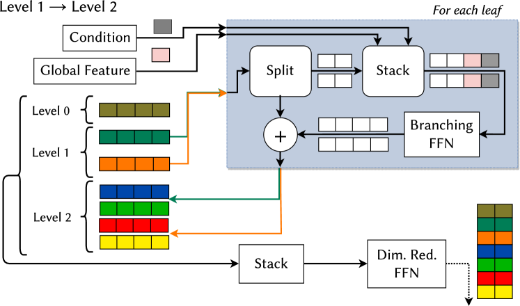
Figure 1: Branching Layer. In this example, the nodes of the 2nd level of the tree are produced and attached as the new leaves. With the nodes from level 1 (dark green / orange) as the parents, the children in level 2 (blue+green / red+yellow) are generated independently: The vector of the parent is split into one part for each of the branches. To each of these vectors, the Global Feature (2) and the global condition vector (here: number of constituents) are concatenated. The Branching FFN maps the vectors to the same size as their parents. Then the feature vector of the parents is added to each of its children. With the new children added as leaves to the tree, all the levels of the tree are stacked up and passed through a Dimensionality Reduction FFN. With each Branching Layer, the number of nodes increases (1 $\to$ 2 $\to$ 2*3 $\to$ 2*3*5) and the number of features decreases (64 $\to$ 33 $\to$ 20 $\to$ 3).

In between the Branching Layers a Message Passing Layer (MPL) passes the information down the tree. In this step, each of the nodes is updated with information from its ancestors. This Ancestor MPL is described in Figure 2.

[capbesideposition=right,top,capbesidewidth=0.6]figure[]

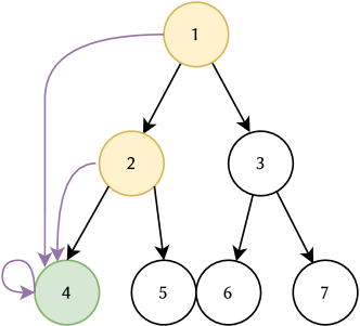
Figure 2: Ancestor Message Passing Layer. The edges in the graph are constructed so that each node receives messages from each of its ancestors as well as itself. In the given example node 4 is updated with the aggregate of the messages from nodes 1, 2 and 4. As a message-passing algorithm, GINConv xu2019powerful – as implemented in PyTorch Geometric pyg – is chosen. For GINConv, the messages are the features of the source node (here: the ancestor). These messages are aggregated by summing over all messages addressed to the target node. These aggregates are added to the feature vector of the target node (scaled with a learnable weight) and passed through an FFN. The nodes are then updated with the output of the FFNs plus, as a residual connection, the original feature vector of the nodes themselves.

A Global Feature Layer is introduced that condenses the information of the current leaves in a single vector: The feature vectors of the leaves are passed through a first FFN, summed up and passed through a second FFN. The resulting vector is then used – together with a global condition vector – to condition the following Branching Layer and Ancestor MPL. The global condition vector contains only the number of constituents in the event. For each of the levels of the tree, first the Global Feature Layer is executed, then the Branching Layer and then the Ancestor MPL.

The FFNs of this model consist of 3 hidden layers of 100 nodes without bias. The first two hidden layers are followed by a Batch Normalization batchnorm layer and LeakyReLU activation with a negative slope of 0.1. As a critic, the MPGAN critic Kansal is used.

2.1 Training

Generator and Critic are trained using the Hinge Hinge loss, with a ratio of 1 to 2 gradient steps. The optimizer for the Generator is Adam with $\beta_{1}=0.9,\beta_{2}=0.999$, a weight decay of $10^{-4}$ and a learning rate of $10^{-5}$. The optimizer for the critic is Adam with $\beta_{1}=0.0,\beta_{2}=0.9$, a weight decay of $10^{-4}$ and a learning rate of $3*10^{-5}$.

2.2 Comparison to tree-GAN

Compared to the model proposed in Shu2019 , DeepTreeGAN introduces some major changes: The branching (Figure 1) uses two FFNs instead of matrix multiplication: one for increasing the number of nodes, the other for reducing the number of features. As the new leaves have the same size as their ancestors, a single Dimensionality Reduction FFN can be applied to all nodes of the tree. After the branching, both models implement a graph convolution step, passing information from the ancestors to their children. In tree-GAN, the leaves are updated using the leaf itself and its ancestors, each multiplied with a separate trainable matrix. In DeepTreeGAN, all nodes in the tree have the same dimension at all times. Thus, all nodes can be updated at the same time, using a single FFN in the Ancestor MPL (Figure 2).

2.3 Preprocessing & Postprocessing

For the training, $\eta^{\mathrm{rel}}$ and $\phi^{\mathrm{rel}}$ are scaled separately to a normal distribution. The ${p}_{\mathrm{T}}^{\mathrm{rel}}$ distribution is transformed using the Box-Cox transformation with standardizing implemented in Sklearn . To produce samples, the inverse scaling is applied to the output of the generator.

3 Results

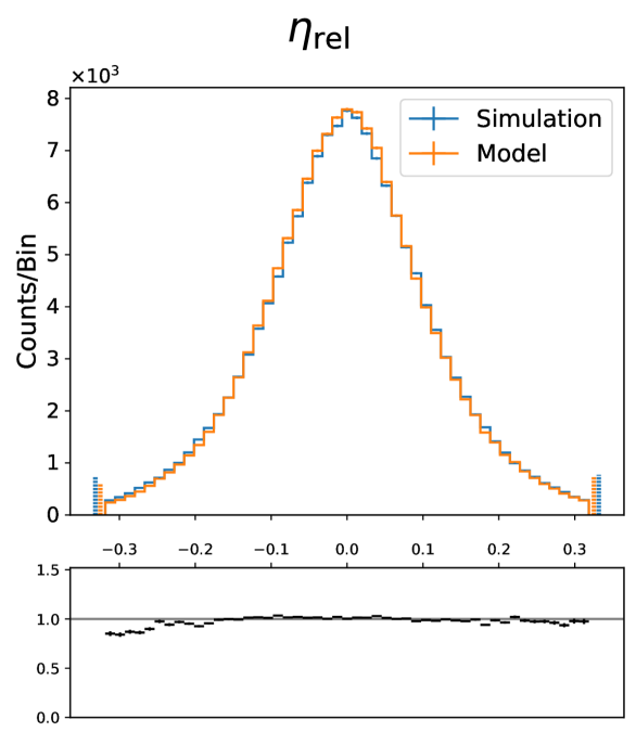
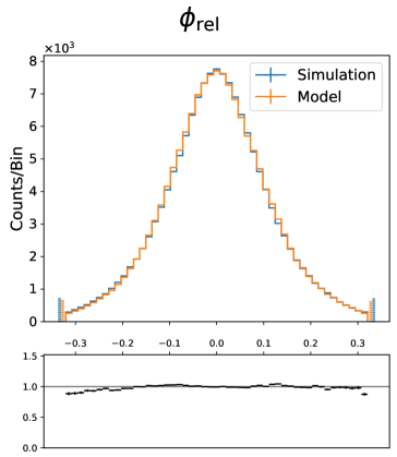
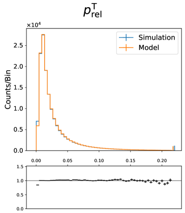
Figure 3: The global particle distributions for the top-quark test dataset, as described in section 1.1.

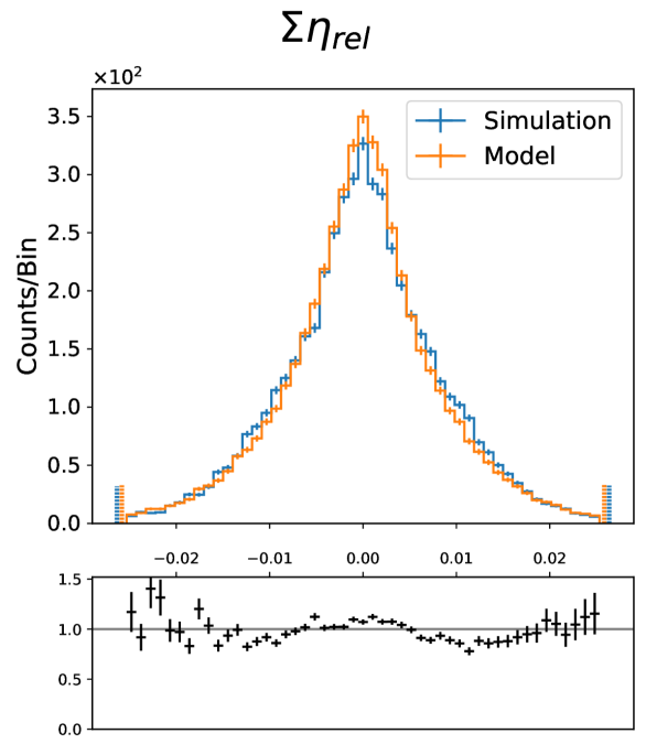
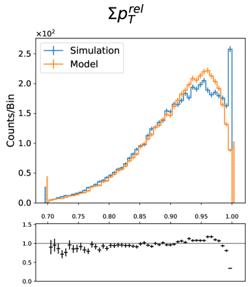
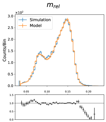
Figure 4: The distributions of the jet variables in the top-quark test dataset.

The variables of the constituents of the top quark dataset are shown in Figure 3. The generated distributions of the constituents closely match the distribution of the data. The jet variables shown in Figure 4 are significantly harder to model. Our model successfully reproduces the double peak structure in the relative jet mass, showing a significant advantage over tree-GAN as shown in (Kansal2022, , Figure 3).

Table 1: Comparison of the proposed DeepTreeGAN to the MPGAN baseline with metrics introduced in Kansal2022 . Significant advantages for a model in a given metric are highlighted bold. The ‘Limit’ row gives the measured in-sample distance by sampling datasets from the training dataset and calculating the metrics. Note that the MPGAN model was selected for $W_{1}^{\mathrm{M}}$, and the testing sample was used to compute the given metrics. The $W_{1}$ metrics are calculated with 10000 samples, FPND is calculated with 50000 samples.

Dataset	Model	$W_{1}^{\mathrm{M}}\times 10^{3}$	$W_{1}^{\mathrm{P}}\times 10^{3}$	$W_{1}^{\mathrm{EFP}}\times 10^{5}$	FPND
Gluon	Limit	$0.7\pm 0.2$	$0.44\pm 0.09$	$0.63\pm 0.07$	$<10^{-3}$
	MPGAN	$\mathbf{0.7}\pm 0.2$	$\mathbf{0.9}\pm 0.3$	$\mathbf{0.7}\pm 0.2$	$\mathbf{0.12}$
	DeepTreeGAN	$1.8\pm 0.2$	$1.6\pm 0.6$	$2.1\pm 0.2$	$0.34$
Light Quarks	Limit	$0.5\pm 0.1$	$0.5\pm 0.1$	$0.46\pm 0.04$	$<10^{-3}$
	MPGAN	$\mathbf{0.7}\pm 0.2$	$4.9\pm 0.5$	$0.7\pm 0.4$	$0.35$
	DeepTreeGAN	$0.9\pm 0.2$	$\mathbf{1.7}\pm 0.3$	$0.9\pm 0.2$	$\mathbf{0.15}$
Top Quarks	Limit	$0.51\pm 0.07$	$0.55\pm 0.07$	$1.1\pm 0.1$	$<10^{-3}$
	MPGAN	$0.6\pm 0.2$	$2.3\pm 0.3$	$2\pm 1$	$0.37$
	DeepTreeGAN	$0.6\pm 0.1$	$\mathbf{1.1}\pm 0.5$	$\mathbf{1.3}\pm 0.3$	$\mathbf{0.14}$

In Table 1 the achieved metrics are shown. While our model shows an advantage over the MPGAN baseline on the top quark dataset and an at least similar performance on the light quarks’ dataset, the performance is worse for the gluon dataset. At the current stage, the generator always produces the full 30 constituents for each of the events. Thus, the performance for events with less than 30 constituents is limited, as is frequently the case for the gluon jets. The models and code are available on GitHub.

4 Conclusion

This paper presents a new model (DeepTreeGAN) for generating large point clouds using a novel upscaling method for point clouds. It successfully replicates the complex distributions of the JetNet datasets with high fidelity (Section 3) and demonstrating its suitability for generating high-dimensional point clouds. The model’s tree-based structure promises good scaling behavior for even larger point clouds, such as particle showers in high-granularity calorimeters. However, the preliminary version presented here uses the MPGAN critic that scales with $\mathcal{O}(\mathrm{points}^{2})$ and thus, requires a new critic with better scaling behavior. In addition, the generator will need to be able to generate a variable number of points for each event, especially for the JetNet datasets with up to 150 particles and the calorimeter use case. This will be the subject of future publications.

References

- (1) S. Agostinelli et al. (GEANT4), Nucl. Instrum. Meth. A 506, 250 (2003)
- (2) J. Albrecht et al. (HEP Software Foundation), Computing and Software for Big Science 3, 7 (2019), 1712.06982
- (3) G. Apollinari, O. BrÃning, T. Nakamoto, L. Rossi, CERN Yellow Report pp. 1–19 (2015), chapter 1 in High-Luminosity Large Hadron Collider (HL-LHC) : Preliminary Design Report, 1705.08830
- (4) C.O. Software, Computing, Tech. rep., Geneva (2022), https://cds.cern.ch/record/2815292
- (5) The CMS collaboration (CMS), The CMS HGCAL detector for HL-LHC upgrade, in 5th Large Hadron Collider Physics Conference (2017), 1708.08234
- (6) I. Goodfellow, J. Pouget-Abadie, M. Mirza, B. Xu, D. Warde-Farley, S. Ozair, A. Courville, Y. Bengio, Commun. ACM 63, 139 (2020), 1406.2661
- (7) D.P. Kingma, M. Welling (2013), 1312.6114
- (8) L. de Oliveira, M. Paganini, B. Nachman, Comput. Software Big Sci. 4 (2017), 1701.05927
- (9) M. Paganini, L. de Oliveira, B. Nachman, Phys. Rev. Lett. 120, 042003 (2018), 1705.02355
- (10) M. Paganini, L. de Oliveira, B. Nachman, Phys. Rev. D 97, 014021 (2018), 1712.10321
- (11) M. Erdmann, L. Geiger, J. Glombitza, D. Schmidt, Comput. Softw. Big Sci. 2, 4 (2018), 1802.03325
- (12) M. Erdmann, J. Glombitza, T. Quast, Comput. Softw. Big Sci. 3, 4 (2019), 1807.01954
- (13) F. Carminati, A. Gheata, G. Khattak, P. Mendez Lorenzo, S. Sharan, S. Vallecorsa, J. Phys. Conf. Ser. 1085, 032016 (2018)
- (14) G. Aad et al., Comput Softw Big Sci 6, 7 (2022)
- (15) B. KÃch, D. KrÃcker, I. Melzer-Pellmann, M. Scham, S. Schnake, A. Verney-Provatas, Jetflow: Generating jets with conditioned and mass constrained normalising flows (2022), 2211.13630
- (16) B. KÃch, D. KrÃcker, I. Melzer-Pellmann, Point cloud generation using transformer encoders and normalising flows (2022), 2211.13623
- (17) S. Schnake, D. KrÃcker, K. Borras, Generating calorimeter showers as point clouds (2022), https://ml4physicalsciences.github.io/2022/files/NeurIPS_ML4PS_2022_77.pdf
- (18) F. Scarselli, M. Gori, A.C. Tsoi, M. Hagenbuchner, G. Monfardini, IEEE Transactions on Neural Networks 20, 61 (2009)
- (19) T.N. Kipf, M. Welling, IEEE Transactions on Neural Networks. 5, 61 (2016), 1609.02907
- (20) D.W. Shu, S.W. Park, J. Kwon, 3d point cloud generative adversarial network based on tree structured graph convolutions (2019), 1905.06292
- (21) R. Kansal, J. Duarte, H. Su, B. Orzari, T. Tomei, M. Pierini, M. Touranakou, J.R. Vlimant, D. Gunopulos (2022), 2106.11535
- (22) T. Sjostrand, S. Mrenna, P.Z. Skands, Comput. Phys. Commun. 178, 852 (2008), 0710.3820
- (23) R. Kansal et al., Jetnet (2022), https://doi.org/10.5281/zenodo.6975118
- (24) R. Kansal et al., Jetnet150 (2022), https://doi.org/10.5281/zenodo.6975117
- (25) R. Kansal, JetNet library for machine learning in high energy physics (2022), https://doi.org/10.5281/zenodo.7140150
- (26) R. Kansal, MPGAN code, https://github.com/rkansal47/MPGAN/tree/neurips21
- (27) K. Xu, W. Hu, J. Leskovec, S. Jegelka, How powerful are graph neural networks? (2019), 1810.00826
- (28) M. Fey, J.E. Lenssen, Fast Graph Representation Learning with PyTorch Geometric, in ICLR Workshop on Representation Learning on Graphs and Manifolds (2019)
- (29) S. Ioffe, C. Szegedy, Batch normalization: Accelerating deep network training by reducing internal covariate shift (2015), 1502.03167
- (30) J.H. Lim, J.C. Ye, Geometric gan (2017), 1705.02894
- (31) F. Pedregosa, G. Varoquaux, A. Gramfort, V. Michel, B. Thirion, O. Grisel, M. Blondel, P. Prettenhofer, R. Weiss, V. Dubourg et al., Journal of Machine Learning Research 12, 2825 (2011)