An Optimisation Approach to Non-Separable Quaternion-Valued Wavelet Constructions

Abstract

We formulate the construction of quaternion-valued wavelets on the plane as a feasibility problem. We refer to this as the quaternionic wavelet feasibility problem. The constraint sets arise from the standard requirements of smoothness, compact support and orthonormality. We solve the resulting feasibility problems by employing the Douglas–Rachford algorithm. From the solutions of the quaternionic wavelet feasibility problem, we derive novel examples of compactly supported, smooth and orthonormal quaternion-valued wavelets on the plane. We also illustrate how a symmetry condition can be added to produce symmetric quaternion-valued scaling functions on the plane.

Keywords:

quaternion $\cdot$ wavelets $\cdot$ Douglas–Rachford $\cdot$ feasibility problem $\cdot$ multiresolution analysis $\cdot$ optimisation

Mathematics Subject Classification (MSC 2020):

42C40 $\cdot$ 65K10 $\cdot$ 65T60 $\cdot$ 90C26

1 Introduction

The inherent limitation of the windowed Fourier transform led researchers to develop what is known today as the wavelet transform. Instead of modulation and translations, a wavelet transform varies the window size using dilations, and slides through the signal using translations. Although the first reference to wavelet goes as far back as 1910 when Haar [1] constructed a class of orthogonal functions known as the Haar wavelets, a major advance in the state of wavelet research was attributed to Morlet and Grossman [27] for rediscovering Calderón’s identity [9] as the continuous wavelet transform (CWT) and showing its applicability to signal analysis. Thereafter, the need for discretising the continuous transform arises, and its realisation has had a long journey exploring from discrete redundant systems to orthonormal wavelet bases. A breakthrough was achieved in 1986 when Mallat [33] and Meyer [34] introduced multiresolution analysis (MRA) as a design method for constructing discrete orthonormal wavelet bases. Eventually, Daubechies [12, 13] assembled a class of smooth compactly supported orthonormal wavelets on the line using MRA.

In recent development, Franklin, Hogan and Tam [23, 24, 25] devised an optimisation approach which has been successful in reproducing Daubechies’ wavelets. Wavelet construction was formulated as a feasibility problem of finding a point on the intersection of constraint sets that model the wavelet design criteria and the conditions of MRA. Feasibility problems are customarily solved using projection algorithms like the method of alternating projections (MAP) and the Douglas–Rachford (DR) scheme, among others. This feasibility approach to wavelet architecture produced nonseparable examples of smooth compactly supported orthonormal wavelets on the plane [24, 25]. Moreover, it makes provision for expanding the design criteria to include other wavelet properties like cardinality and symmetry [14, 16, 17, 18, 19].

In applications, the prevalent higher-dimensional signals are vector-valued. Dealing with such signals—like colour images—requires more sophisticated and higher-dimensional extensions of wavelet transforms. More precisely, a typical colour image is viewed as a three-channel signal on the plane, where these channels are customarily the red, green and blue (RGB) components of the pixels. Alternative colour image models include the luminance–chrominance (YUV) and the cyan–magenta–yellow–key (CMYK) that use three and four channels, respectively. Most contemporary methods for handling colour images rely on independently analysing each channel. This approach often neglects or minimizes the potential correlations between these channels. It is more advantageous to encode the pixel components using higher-dimensional algebras that are able to harness these inter-channel correlations. In the case of colour images with three or four channels, the algebra of quaternions is considered suitable for this purpose [28, 36, 38].

While a plethora of research address quaternionic extensions of wavelet transforms, a rather limited number of scholarly works are devoted to the development of true quaternionic wavelets. Within their comprehensive survey paper concerning the development of quaternionic wavelet transforms (QWT), Fletcher and Sangwine [22] noted that most of these constructions were only derived from real or complex filter coefficients and are just separate discrete wavelet transforms in disguise. They further went on to conclude that the research works due to Hogan and Moris [29, 35], and Ginzberg and Walden [26] are among the few that attempted to develop true QWT. Hogan and Morris derived fundamental analogues of classical wavelet theory including the basic results required to construct orthonormal quaternion-valued wavelets on the plane with compact support and prescribed regularity based on quaternionic MRA. However, no such wavelets have been created. Recently, Fletcher [21] expanded Ginzberg’s theory to provide examples of quaternion-valued scaling filters on the line.

In this paper, we build on the quaternionic wavelet theory developed by Hogan and Morris [29, 35]. Drawing inspiration from the complex-valued case [23, 24, 25], we formulate quaternionic wavelet construction as a feasibility problem and solve it to obtain novel examples of compactly supported, smooth and orthonormal quaternion-valued wavelets on the plane.

This paper is organised as follows. In the remainder of Section 1, we fix notation and introduce relevant concepts in the algebra of quaternions, quaternionic Fourier transforms, and optimisation theory. Section 2 contains a brief discussion of quaternionic MRA, scaling functions and wavelets. Here we revisit important results by Hogan and Morris that are relevant to the construction of compactly support, smooth and orthonormal quaternion-valued wavelets based on a quaternionic MRA. We add point symmetry as a design criterion for the scaling function. Section 3 details the formulation of quaternionic wavelet architecture as a feasibility problem. In Section 4, we list the constraint sets that comprise the quaternionic wavelet feasibility problem and derive their respective projectors. Finally, in Section 5, we solve specific cases of the quaternionic wavelet feasibility problem using the Douglas–Rachford algorithm.

1.1 Basic notation

If $z\in\mathbb{C}$, then $\Re(z)$ is its real part and $\Im(z)$ is its imaginary part. We would like to view $\mathbb{C}^{d}$ as a real inner product space with $\langle\cdot,\cdot\rangle_{\mathbb{R}}:\mathbb{C}^{d}\times\mathbb{C}^{d}\to\mathbb{R}$ defined by

$$\langle x,y\rangle_{\mathbb{R}}=\sum_{k=1}^{d}\big{(}\langle\Re(x_{k}),\Re(y_{k})\rangle+\langle\Im(x_{k}),\Im(y_{k})\rangle\big{)}.$$

The collection of $a\times b$ matrices with complex entries is denoted by $\mathbb{C}^{a\times b}$, and the collection of $c\times c$ unitary matrices is $\mathcal{U}(c)$. Moreover, $I_{d}\in\mathbb{C}^{d\times d}$ is the identity matrix. If $v_{1},v_{2},\ldots,v_{d}\in\mathbb{C}$, then $\mbox{diag}(v_{1},v_{2},\ldots,v_{d})$ denotes the $d\times d$ diagonal matrix with the vector $(v_{1},v_{2},\ldots,v_{d})$ on its diagonal. We also define $\mathbb{C}^{a\times b}\otimes\mathbb{C}^{c\times d}$ to be the set of all block diagonal matrices in $\mathbb{C}^{(a+c)\times(b+d)}$ formed by taking the direct sum of $M_{1}\in\mathbb{C}^{a\times b}$ and $M_{2}\in\mathbb{C}^{c\times d}$. If $A\in\mathbb{C}^{a\times b}$, then $A_{ij}$ or $A[i,j]$ interchangeably denotes the $(i,j)$-entry of $A$. For matrices $A,B\in\mathbb{C}^{d\times d}$, $A^{\ast}$ is the Hermitian conjugate of $A$, and the Frobenius inner product of $A$ and $B$ is defined by $\langle A,B\rangle_{F}=\operatorname{Tr}(A^{\ast}B)=\sum_{i,k=1}^{d}\overline{A_{ik}}B_{ik}$. The Frobenius matrix norm is given by

$$\|A\|_{F}^{2}=\sum_{i,k=1}^{d}|A_{ik}|^{2}=\sum_{i,k=1}^{d}\big{(}(\Re(A_{ik}))^{2}+(\Im(A_{ik}))^{2}\big{)}.$$

1.2 Quaternion algebra

Let $\mathbb{R}_{2}:=\{x=x_{0}+x_{1}e_{1}+x_{2}e_{2}+x_{12}e_{12}\,:\,x_{0},x_{1},x_{2},x_{12}\in\mathbb{R},\,e_{1}^{2}=e_{2}^{2}=e_{12}^{2}=e_{1}e_{2}e_{12}=-1\}$ be the set of quaternions. Given $x=x_{0}+x_{1}e_{1}+x_{2}e_{2}+x_{12}e_{12}\in\mathbb{R}_{2}$, we call $x_{0}$ the real part of $x$, and $x_{1},x_{2},x_{12}$ the imaginary parts of $x$. If $x_{0}=0$ then $x$ is a pure quaternion. If $x_{0}=x_{12}=0$ then $x$ is a vector. If $x_{1}=x_{2}=x_{12}=0$, then $x$ is a scalar. We may also decompose $\mathbb{R}_{2}$ in this manner:

$$\mathbb{R}_{2}=\Lambda_{0}\oplus\Lambda_{1}\oplus\Lambda_{2},$$

where $\Lambda_{0}:=\mathbb{R}$, $\Lambda_{1}:=\{x_{1}e_{1}+x_{2}e_{2}:x_{1},x_{2}\in\mathbb{R}\}$, and $\Lambda_{2}:=\{x_{12}e_{12}:x_{12}\in\mathbb{R}\}$. We write $[x]_{k}$ to refer to the $\Lambda_{k}$-part of $x=x_{0}+x_{1}e_{1}+x_{2}e_{2}+x_{12}e_{12}\in\mathbb{R}_{2}$. Note that $\Lambda_{0}$ is the set of scalars, and $\Lambda_{1}$ is the collection of vectors. In view of $\Lambda_{1}$, we consider $\mathbb{R}^{2}$ to be embedded in $\mathbb{R}_{2}$ as vectors. If $x,y\in\mathbb{R}_{2}$ are vectors, then

$$x^{2}=-|x|^{2}\text{~{}~{}and~{}~{}}xy=-\langle x,y\rangle+x\wedge y\in\Lambda_{0}\oplus\Lambda_{1},$$

where $\langle\cdot,\cdot\rangle$ is the usual inner product in $\mathbb{R}^{2}$ and $x\wedge y:=e_{12}(x_{1}y_{2}-x_{2}y_{1})$ is the wedge product of $x$ and $y$.

We remark that a quaternion $x=x_{0}+x_{1}e_{1}+x_{2}e_{2}+x_{12}e_{12}$ has a polar form representation given by

$$x=|x|e^{\mu_{x}\phi_{x}}=(\cos(\phi_{x})+|x|\mu_{x}\sin(\phi_{x}))$$ (1)

where

$$\begin{cases}|x|&=\sqrt{x_{0}^{2}+x_{1}^{2}+x_{2}^{2}+x_{12}^{2}}\\ \mu_{x}&=\dfrac{x_{1}e_{1}+x_{2}e_{2}+x_{12}e_{12}}{\sqrt{x_{1}^{2}+x_{2}^{2}+x_{12}^{2}}}\\ \phi_{x}&=\arctan\left(\frac{\sqrt{x_{1}^{2}+x_{2}^{2}+x_{12}^{2}}}{x_{0}}\right)\end{cases}$$ (2)

where $\mu_{x}\phi_{x}$ is a pure quaternion.

We further define $x_{s}:=x_{0}+x_{12}e_{12}$ and $x_{v}=x_{1}e_{1}+x_{2}e_{2}$ as the spinor and vector parts of $x$, respectively. The spinor and vector parts of any $x,y\in\mathbb{R}_{2}$ satisfy the following commutation relations [29, 35]:

1. $x_{s}y_{s}=y_{s}x_{s}$,

2. $x_{s}y_{v}=y_{v}\overline{x_{s}}$,

3. $x_{v}y_{v}=-e_{1}y_{v}x_{v}e_{1}=-e_{2}y_{v}x_{v}e_{2}$.

Moreover, for a function $f:X\rightarrow\mathbb{R}_{2}$ where $X\subseteq\mathbb{R}^{2}$, we write $f(x)=f_{0}(x)+f_{1}(x)e_{1}+f_{2}(x)+f_{12}(x)$ where $f_{0},f_{1},f_{2},f_{12}:X\to\mathbb{R}$. The spinor part $f_{s}$ of $f$ is defined as $f_{s}(x):=(f(x))_{s}=f_{0}(x)+f_{12}(x)e_{12}$ while its vector part $f_{v}$ is given by $f_{v}(x):=(f(x))_{v}=f_{1}(x)e_{1}+f_{2}(x)e_{2}$. We further define the spinor-vector (SV) matrix of a function $f:\mathbb{R}^{2}\to\mathbb{R}_{2}$ by

$$[f(x)]:=\begin{bmatrix}f_{s}(x)&f_{v}(x)\\ f_{v}(-x)&f_{s}(-x)\end{bmatrix}.$$

In general, a matrix $A\in\mathbb{R}_{2}^{2\times 2}$ (not necessarily attached to a quaternion-valued function) is a spinor-vector (SV) matrix if it is of the form

$$A=\begin{bmatrix}s_{1}&v_{1}\\ v_{2}&s_{2}\end{bmatrix}\mbox{ where }s_{1},s_{2}\in\Lambda_{0}\oplus\Lambda_{2}\mbox{ and }v_{1},v_{2}\in\Lambda_{1}.$$

Henceforth, we let $\mathsf{S}$ to be the set of all $SV$ matrices. Furthermore, if we define

$$Z:=\left\{x=\begin{bmatrix}x_{s}&x_{v}\end{bmatrix}^{T}:x_{s}\in\Lambda_{0}\oplus\Lambda_{2},\,x_{v}\in\Lambda_{1}\right\}$$

then $A\in\mathsf{S}$ determines a linear transformation on $Z$. In fact, $Z$ is a right inner product module with inner product $\langle x,y\rangle=\overline{x_{s}}y_{s}+\overline{x_{v}}y_{v}$ satisfying $\overline{\langle x,y\rangle}=\langle y,x\rangle$, $\langle x,ya\rangle=\langle x,y\rangle a$ and $\langle xa,y\rangle=\overline{a}\langle x,y\rangle$ for all $x,y\in Z$, $a\in\Lambda_{0}\oplus\Lambda_{2}$. Moreover, if $A^{\ast}=\overline{A}^{T}$ is the Hermitian adjoint of $A$, then $\langle Ax,y\rangle=\langle x,A^{\ast}y\rangle$. We say that $A$ is self-adjoint whenever $A=A^{\ast}$, i.e., $s_{1},s_{2}\in\mathbb{R}$ and $v_{2}=-v_{1}$. We also define an eigenvector $x$ of $A$ to be a nonzero vector $x=\begin{bmatrix}x_{s}&x_{v}\end{bmatrix}^{T}\in Z$ such that $Ax=x\lambda$, where $\lambda\in\Lambda_{0}\oplus\Lambda_{2}$ is the eigenvalue. The two eigenvalues of $A$ are computed using the formula

$$\lambda=\frac{s_{1}+\overline{s_{2}}\pm\sqrt{(s_{1}-\overline{s_{2}})^{2}+4v_{1}v_{2}}}{2}.$$ (3)

In addition, if $A$ is self-adjoint then its eigenvalues are real. We also say that $A$ is positive definite if $\langle Ax,x\rangle>0$ for all nonzero $x\in Z$. Furthermore, $A$ is positive definite if and only if all of its eigenvalues are positive. Given two self-adjoint $A,B\in\mathsf{S}$, we say $A<B$ whenever $\langle Ax,x\rangle<\langle Bx,x\rangle$ for every $x\in Z$. For a comprehensive discussion on the linear algebra of SV matrices, refer to [29, Section 1.2] or [35, Section 1.5].

We remark that $\Lambda_{0}\oplus\Lambda_{2}$ is a subalgebra of $\mathbb{R}_{2}$ and if we define $\phi:\Lambda_{0}\oplus\Lambda_{2}\to\mathbb{C}$ by $\phi(x_{0}+x_{12}e_{12})=x_{0}+x_{12}i$, then $\phi$ is an isomorphism. Thus, $\Lambda_{0}\oplus\Lambda_{2}\cong\mathbb{C}$. Throughout this manuscript, we use $\mathbb{C}$ and $\Lambda_{0}\oplus\Lambda_{2}$ interchangeably and apply theorems valid for $\mathbb{C}^{d}$ to $(\Lambda_{0}\oplus\Lambda_{2})^{d}$.

Finally, we denote the collection of $m\times m$ SV-block matrices by

$$\mathsf{S}^{m\times m}:=\left\{\begin{bmatrix}A_{11}&\cdots&A_{1m}\\ \vdots&\ddots&\vdots\\ A_{m1}&\cdots&A_{mm}\end{bmatrix}\ :\ A_{ij}\in\mathsf{S}\mbox{ for }i,j\in\{1,2,\ldots,m\}\right\},$$

and by $\mathcal{U}^{m\times m}$ the set of unitary $m\times m$ SV-block matrices.

1.3 Quaternionic Fourier transform

Definition 1.1.

Let $f\in L^{1}(\mathbb{R}^{2},\mathbb{R}_{2})$. The quaternionic Fourier transform $\operatorname{\mathcal{F}_{2}^{+}}f$ of $f$ is given by

$$\operatorname{\mathcal{F}_{2}^{+}}f(\xi):=\hat{f}(\xi):=\int_{\mathbb{R}^{2}}e^{2\pi\xi\wedge x}f(x)\,dx.$$

In this manuscript, we use $\operatorname{\mathcal{F}_{2}^{+}}$ or $\hat{f}$ interchangeably to denote the Fourier transform of $f$.

Proposition 1.2.

Let $f,g\in L^{2}(\mathbb{R}^{2},\mathbb{R}_{2})$. The quaternionic Fourier transform satisfies the following properties:

1. $\langle f,g\rangle=\langle\operatorname{\mathcal{F}_{2}^{+}}{f},\operatorname{\mathcal{F}_{2}^{+}}g\rangle$,

2. $\|f\|_{2}=\|\operatorname{\mathcal{F}_{2}^{+}}f\|_{2}$,

3. $\operatorname{\mathcal{F}_{2}^{+}}(f(\cdot-a))(\xi)=e^{2\pi\xi\wedge a}\operatorname{\mathcal{F}_{2}^{+}}f(\xi)$ ,

4. $\operatorname{\mathcal{F}_{2}^{+}}(e^{2\pi\cdot\wedge a}f)(\xi)=(\operatorname{\mathcal{F}_{2}^{+}}f)(\xi-a)$,

5. $\displaystyle\operatorname{\mathcal{F}_{2}^{+}}(f(b\cdot))(\xi)=\frac{1}{b^{2}}\operatorname{\mathcal{F}_{2}^{+}}f\left(\frac{\xi}{b}\right)$,

6. $(\operatorname{\mathcal{F}_{2}^{+}})^{2}=\operatorname{Id}$,

where $a\in\mathbb{R}^{2}$ and $b>0$. Furthermore, if $f\ast g$ is the convolution of $f$ and $g$, then

$$[\operatorname{\mathcal{F}_{2}^{+}}(f\ast g)(\xi)]=[\operatorname{\mathcal{F}_{2}^{+}}f(\xi)][\operatorname{\mathcal{F}_{2}^{+}}g(\xi)]$$ (4)

which is also referred to as the convolution theorem for the quaternionic Fourier transform.

The convolution theorem in (4) is due to Hogan and Morris [30, Theorem 2.16] and is understood in terms of spinor-vector matrices. It is also worth noting the convolution of two functions is defined similarly as in the classical setting with a caveat that, in general, $f\ast g\neq g\ast f$. For a more elaborate discussion on the quaternionic Fourier transform, refer to [29, 35].

We note in the next proposition that the SV matrix of the integral kernel of the quaternionic Fourier transform commutes with the SV matrix of any quaternion-valued function.

Proposition 1.3.

If $f:\mathbb{R}^{2}\to\mathbb{R}_{2}$, then for any $x,\xi\in\mathbb{R}^{2}$ we have

$$[e^{2\pi\xi\wedge x}][f(x)]=[f(x)][e^{2\pi\xi\wedge x}].$$

Proof.

See [35, Lemma 1.19]. ∎

1.4 Feasibility problems and the Douglas–Rachford algorithm

Since our construction approach relies heavily on optimisation, we first revisit relevant concepts on optimisation concerning feasibility problems and how to solve them.

A feasibility problem is a special case of an optimisation problem that involves finding a point in the intersection of a finite family of sets. More succinctly, for a fixed $r\in\mathbb{N}$ and given sets $K_{1},K_{2},\dots,K_{r}$ contained in a Hilbert space $\mathcal{H}$, the corresponding feasibility problem is given by:

$$\text{find~{}}x^{\ast}\in K:=\bigcap_{j=1}^{r}K_{j}.$$

In the literature, projection algorithms are often used to solve feasibility problems. The Douglas–Rachford (DR) algorithm [20] stands as a well-known example of projection algorithm that solves a two-set feasibility problem. It has been observed to demonstrate empirical effectiveness even in nonconvex settings [2, 3, 4, 7, 8, 11].

The DR scheme exploits the concept of projectors and reflectors. If $C$ is a nonempty subset of $\mathcal{H}$, the projector onto $C$ is the set-valued operator $P_{C}\colon\mathcal{H}\rightrightarrows C$ defined by

$$P_{C}(x)=\{c\in C:\|x-c\|=\inf_{z\in C}\|x-z\|\};$$

and the reflector with respect to $C$ is the set-valued operator $R_{C}\colon\mathcal{H}\rightrightarrows\mathcal{H}$ defined by

$$R_{C}:=2P_{C}-\operatorname{Id}.$$

An element of $P_{C}(x)$ is called a projection of $x$ onto $C$. Similarly, an element of $R_{C}(x)$ is called a reflection of $x$ with respect to $C$. The use of “$\rightrightarrows$” is to denote that an operator is possibly set-valued. In the next proposition, we write down examples of projectors that will be frequently referred to throughout this manuscript.

Proposition 1.4.

Let $\mathcal{H}_{1},\mathcal{H}_{2}$ be finite-dimensional Hilbert spaces, $\mathsf{S}^{n\times n}$ be the collection of $n$-by-$n$ SV-block matrices, and $\mathcal{U}^{n\times n}$ be the set of unitary $n\times n$ SV-block matrices.

1. If $T:\mathcal{H}_{1}\to\mathcal{H}_{2}$ is linear, $C=\operatorname{null}T:=\{x\in\mathcal{H}_{1}\,:\,Tx=0\}$ and $TT^{\ast}$ is invertible, then

   $$P_{C}(x)=x-T^{\ast}(TT^{\ast})^{-1}T(x)\text{ for all }x\in\mathcal{H}_{1}.$$

2. If $0\neq a\in\mathcal{H}_{1}$, $\beta\in\mathbb{R}$ and $C=\{z\in\mathcal{H}_{1}\,:\,\langle a,z\rangle=\beta\}$, then for all $x\in\mathcal{H}_{1}$

   $$P_{C}(x)=x-\frac{\langle a,x\rangle-\beta}{\|a\|^{2}}a.$$

3. If $C=\mathcal{B}(z,\delta)\subset\mathcal{H}_{2}$, then

   $$P_{C}(x)=\begin{cases}x,&\text{if~{}}\|x-z\|\leq\delta\\ z+\frac{\delta}{\|x-z\|}(x-z)&\text{if~{}}\|x-z\|>\delta.\end{cases}$$

4. If $A\in\mathsf{S}^{n\times n}$ then $P_{\mathcal{U}^{n\times n}}(A)=\{UV^{\ast}\,:\,A=U\Sigma V^{\ast}\text{ is an SVD}\}.$

5. Let $a\in\mathsf{S}$, $b\in\mathsf{S}^{1\times(n-1)}$, $c\in\mathsf{S}^{(n-1)\times 1}$, $D\in\mathsf{S}^{(n-1)\times(n-1)}$ and $A=\begin{bmatrix}a&b\\ c&D\end{bmatrix}.$ Then

   $$P_{[1]\otimes\mathcal{U}^{(n-1)\times(n-1)}}(A)=\left\{\begin{bmatrix}[1]&d^{T}\\ d&\tilde{D}\end{bmatrix}:d=0\in\mathsf{S}^{(n-1)\times 1},\tilde{D}\in P_{\mathcal{U}^{(n-1)\times(n-1)}}(D)\right\}.$$

6. Let $Q$ be a countably finite index set, $(\mathsf{S}^{n\times n})^{Q}:=\{\mathbf{B}=(B_{j})_{j\in Q}\,:\;B_{j}\in\mathsf{S}^{n\times n}\ \forall j\in Q\}$ and $(\mathcal{U}^{n\times n})^{Q}:=\{\mathbf{B}=(B_{j})_{j\in Q}\,:\,B_{j}\in\mathcal{U}^{n\times n}\ \forall j\in Q\}$. For any $\mathbf{V}\in(\mathsf{S}^{n\times n})^{Q}$,

   $$\mathbf{W}=(W_{j})_{j\in Q}\in P_{({\mathcal{U}^{n\times n}})^{Q}}(\mathbf{V})\iff W_{j}\in P_{\mathcal{U}^{n\times n}}(V_{j})\text{~{}~{}for all ~{}}j\in Q.$$

7. Let $0\neq\mathbf{a}\in\mathbb{C}^{d}$, $b\in\mathbb{C}$, $\epsilon\geq 0$ and $C:=\{\mathbf{z}\in\mathbb{C}^{d}\,:\,|\langle\mathbf{a},\mathbf{z}\rangle+b|\leq\epsilon\}$. If $\beta(\mathbf{z})=\frac{\epsilon(\langle\mathbf{a},\mathbf{z}\rangle+b)}{|\langle\mathbf{a},\mathbf{z}\rangle+b|}$, then $P_{C}(z)=\mathbf{p}$ where

   $$\mathbf{p}=\begin{cases}\mathbf{z}&\text{if~{}}|\langle\mathbf{a},\mathbf{z}\rangle+b|\leq\epsilon\\ \mathbf{z}+\frac{\beta(\mathbf{z})-\langle\mathbf{a},\mathbf{z}\rangle-b}{\|\mathbf{a}\|^{2}}\mathbf{a}&\text{if~{}}|\langle\mathbf{a},\mathbf{z}\rangle+b|>\epsilon.\end{cases}$$

Proof.

For (a), see [5, Example 29.17]. For (b)–(c), see [10, Section 4.1]. For (d), see [15, Corollary 6.30]. Statements (e) and (f) directly follow from (d). Lastly, for (g), see [15, Proposition 1.8]. ∎

We now introduce the DR algorithm.

Definition 1.5.

Given two nonempty subsets $A$ and $B$ of $\mathcal{H}$, the DR operator $T_{A,B}$ is defined as

$$T_{A,B}:=\frac{\operatorname{Id}+R_{B}R_{A}}{2}.$$

It is worth noting (see [6, Equations (20)–(23)]) that if $P_{A}$ is single-valued, then

$$T_{A,B}=\operatorname{Id}-P_{A}+P_{B}R_{A}\text{~{}~{}and~{}~{}}P_{A}(\operatorname{Fix}T_{A,B})=A\cap B.$$

If $A$ and $B$ are closed convex subsets of $\mathcal{H}$ with $A\cap B\neq\varnothing$, then, for any $x_{0}\in\mathcal{H}$, the sequence $(x_{n})_{n\in\mathbb{N}}$ generated by $x_{n+1}=T_{A,B}(x_{n})$ converges weakly to a point $x^{\ast}\in\operatorname{Fix}T_{A,B}$, and the shadow sequence $(P_{A}(x_{n}))_{n\in\mathbb{N}}$ converges weakly to $P_{A}(x^{\ast})\in A\cap B$ [32, 40].

Although originally formulated for two-set feasibility problems, the DR algorithm has been adapted to solve many-set feasibility problems by employing Pierra’s product space reformulation [37] (among other extensions). To be more precise, given $K_{1},K_{2},\dots,K_{r}\subseteq\mathcal{H}$, with corresponding projectors $P_{K_{1}},P_{K_{2}},\dots,P_{K_{r}}$, the sets $C$ and $D$ in the product Hilbert space $\mathcal{H}^{r}$ are defined by

$$C :=K_{1}\times K_{2}\times\dots\times K_{r}\text{ and}$$ (5a)

$$D :=\{(x_{1},x_{2},\dots,x_{r})\in\mathcal{H}^{r}:x_{1}=x_{2}=\cdots=x_{r}\}.$$ (5b)

The $r$-set feasibility problem is equivalent to the two-set feasibility problem on $C$ and $D$ in the sense that

$$x^{\ast}\in\bigcap_{j=1}^{r}K_{j}\ \iff\mathbf{x}^{\ast}:=(x^{\ast},x^{\ast},\dots,x^{\ast})\in C\cap D.$$ (6)

Furthermore, the projectors onto $C$ and $D$ are given by

$$P_{C}(\mathbf{x})=P_{K_{1}}(x_{1})\times P_{K_{2}}(x_{2})\times\dots\times P_{K_{r}}(x_{r})\text{ and }\,P_{D}(\mathbf{x})=\left(\frac{1}{r}\sum_{j=1}^{r}x_{j},\frac{1}{r}\sum_{j=1}^{r}x_{j},\dots,\frac{1}{r}\sum_{j=1}^{r}x_{j}\right)$$

for any $\mathbf{x}=(x_{1},x_{2},\dots,x_{r})\in\mathcal{H}^{r}$; see, e.g., [5, Proposition 29.3 and Proposition 26.4(iii)].

The pseudocode for implementing the DR is outlined in Algorithm 1.This readily applies to the a wavelet feasibility problem where $C$ and $D$ are as in (5a) and (5b), respectively.

input : $x_{0}\in\mathcal{H}$

Compute $p_{0}\in P_{D}(x_{0})$;

while stopping criteria not satisfied do

       Compute $x_{k+1}$ such that $x_{k+1}\in x_{k}+P_{C}(2p_{k}-x_{k})-p_{k}$;

       Compute $p_{k+1}$ such that $p_{k+1}\in P_{D}(x_{k+1})$;

       Update $x_{k}=x_{k+1}$;

      

end while

output : $p_{k}$

Algorithm 1 DR

2 Quaternionic wavelets on the plane

In this section, we recall important results by Hogan and Morris [29, 35] that are required to construct orthonormal quaternion-valued wavelets on the plane with compact support and prescribed regularity based on quaternionic multiresolution analysis.

2.1 MRA, scaling function and wavelets

Definition 2.1.

A multiresolution analysis (MRA) for $L^{2}(\mathbb{R}^{2},\mathbb{R}_{2})$ is a collection of closed right linear $\mathbb{R}_{2}$-submodules $(V_{j})_{j\in\mathbb{Z}}$ of $L^{2}(\mathbb{R}^{2},\mathbb{R}_{2})$ and a function $\varphi\in V_{0}$ such that the following conditions hold:

1. $V_{j}\subset V_{j+1}$ for all $j\in\mathbb{Z}$,

2. $\overline{\bigcup_{j\in\mathbb{Z}}V_{j}}=L^{2}(\mathbb{R}^{2},\mathbb{R}_{2})$ and $\,\bigcap_{j\in\mathbb{Z}}V_{j}=\{0\}$,

3. $f(\cdot)\in V_{0}$ if and only if $f(\cdot-k)\in V_{0}$ for all $k\in\mathbb{Z}^{2}$,

4. $f(\cdot)\in V_{0}$ if and only if $f(2^{j}\cdot)\in V_{j}$ for all $j\in\mathbb{Z}$, and

5. $\{\varphi(\cdot-k)\}_{k\in\mathbb{Z}^{2}}$ forms an orthonormal basis for $V_{0}$.

The function $\varphi\in V_{0}$ in Definition 2.1 is called the scaling function. Combining conditions (d)–(e) of Definition 2.1, we see that $\varphi(\frac{x}{2})\in V_{-1}\subset V_{0}$ and there exists $(a_{k}^{0})_{k\in\mathbb{Z}^{2}}\in\ell^{2}(\mathbb{Z}^{2},\mathbb{R}_{2})$ such that

$$\frac{1}{4}\varphi\left(\frac{x}{2}\right)=\sum_{k\in\mathbb{Z}^{2}}\varphi(x-k)a_{k}^{0}.$$ (7)

We refer to (7) the scaling or dilation equation. In the Fourier domain, this is best viewed in terms of the spinor-vector matrix.

Proposition 2.2.

Let $\varphi\in L^{2}(\mathbb{R}^{2},\mathbb{R}_{2})$ be a scaling function as in Definition 2.1. Then (7) is equivalent to

$$[\hat{\varphi}(2\xi)]=[\hat{\varphi}(\xi)][m_{0}(\xi)]$$ (8)

where $m_{0}(\xi)=\sum_{k\in\mathbb{Z}^{2}}e^{2\pi\xi\wedge k}a_{k}^{0}$.

Proof.

See [29, Lemma 2] or [35, Lemma 4.1]. ∎

We call $m_{0}$ the scaling filter. Repeated application of (8) yields

$$[\hat{\varphi}(\xi)]=\left[\varphi\left({\frac{\xi}{2^{J}}}\right)\right]\left[m_{0}\left({\frac{\xi}{2^{J}}}\right)\right]\left[m_{0}\left({\frac{\xi}{2^{J-1}}}\right)\right]\cdots\left[m_{0}\left({\frac{\xi}{2}}\right)\right],$$

and the infinite product $[\hat{\varphi}(\xi)]=\prod_{j=1}^{\infty}\left[m_{0}\left(\frac{\xi}{2^{j}}\right)\right]$ gives a way to recover $\varphi$ from $m_{0}$ whenever the product converges.

We further note that condition (d) in Definition 2.1 may be generalised to $f(\cdot)\in V_{0}\Longleftrightarrow f(M^{j}\cdot)\in V_{j+1}$ for all $j\in\mathbb{Z}$, where $M$ is a $2\times 2$ dilation matrix, i.e., $M$ has integer entries and its eigenvalues are greater than one in absolute value. And for any dilation matrix $M$, there are $\det(M)$ cosets of $M\mathbb{Z}^{2}$ in $\mathbb{Z}^{2}$ [31, Proposition 2.1.1]. For our purpose, $M=2I_{2}$ and $\det(M)-1=3$. Thus, we have three other cosets of $2\mathbb{Z}^{2}$ in $\mathbb{Z}^{2}$ and each of them corresponds to a wavelet function (or simply wavelet) $\psi^{\varepsilon}$ ($\varepsilon\in\{1,2,3\}$) such that

$$\left\{2^{j}\psi^{\varepsilon}(2^{j}\cdot-k)\ :\ j\in\mathbb{Z},\ k\in\mathbb{Z}^{2},\ \varepsilon\in\{1,2,3\}\right\}$$

forms an orthonormal basis for $L^{2}(\mathbb{R}^{2},\mathbb{R}_{2})$.

Since each $\psi^{\varepsilon}(\frac{x}{2})\in V_{-1}\subset V_{0}$, for each $\varepsilon\in\{1,2,3\}$, there exists $(a_{k}^{\varepsilon})_{k\in\mathbb{Z}^{2}}\in\ell^{2}(\mathbb{Z}^{2},\mathbb{R}_{2})$ such that

$$\frac{1}{4}\psi^{\varepsilon}\left(\frac{x}{2}\right)=\sum_{k\in\mathbb{Z}^{2}}\varphi(x-k)a_{k}^{\varepsilon}.$$ (9)

Taking the quaternionic Fourier transform of both sides of (9) yields an equivalent expression in terms of spinor-vector matrices.

Proposition 2.3.

Let $\varphi\in L^{2}(\mathbb{R}^{2},\mathbb{R}_{2})$ be a scaling function as in Definition 2.1 and $\psi^{\varepsilon}$ be the associated wavelets ($\varepsilon\in\{1,2,3\}$). Then (9) is equivalent to

$$[\hat{\psi}^{\varepsilon}(2\xi)]=[\hat{\varphi}(\xi)][m_{\varepsilon}(\xi)]$$ (10)

where $m_{\varepsilon}(\xi)=\sum_{k\in\mathbb{Z}^{2}}e^{2\pi\xi\wedge k}a_{k}^{\varepsilon}$, for each $\varepsilon\in\{1,2,3\}$.

Proof.

See [29, Lemma 2] or [35, Lemma 4.1]. ∎

2.2 Quaternionic wavelet design conditions

In some instances, we write $\psi^{0}=\varphi$ for convenience in collectively referring to the scaling function and its associated wavelets in the wavelet ensemble $\{\psi^{\varepsilon}\}_{\varepsilon=0}^{3}$. We also adopt the notation

$$\psi_{jk}^{\varepsilon}(x):=2^{j}\psi^{\varepsilon}(2^{j}x-k)$$

to refer to the normalised versions of the translated and dilated scaling function and wavelets. With this notation, $\{\varphi_{jk}\}_{k\in\mathbb{Z}^{2}}$ and $\{\psi_{jk}^{\varepsilon}\,:\,\varepsilon\in\{1,2,3\}\}_{k\in\mathbb{Z}^{2}}$ are orthonormal bases for $V_{j}$ and $W_{j}$, respectively.

2.2.1 Orthogonality

We first revisit the necessary and sufficient conditions for the orthonormality of the shifts of the scaling function and the wavelets. Henceforth, we let

$$V^{2}:=\{v_{0}:=(0,0),v_{1}:=(1,0),v_{2}:=(0,1),v_{3}:=(1,1)\}$$ (11)

be the vertices of the unit square in $\mathbb{R}^{2}$.

Proposition 2.4.

Let $\varphi$ be a scaling function that generates an MRA for $L^{2}(\mathbb{R}^{2},\mathbb{R}_{2})$ where $\{\varphi_{0k}\}_{k\in\mathbb{Z}^{2}}$ forms an orthonormal basis for $V_{0}$. If $m_{0}$ is the scaling filter associated with $\varphi$, then

$$\sum_{j=0}^{3}\left[m_{0}\left(\xi+{\textstyle\frac{v_{j}}{2}}\right)\right]^{\ast}\left[m_{0}\left(\xi+{\textstyle\frac{v_{j}}{2}}\right)\right]=I_{2}$$ (12)

for almost every $\xi\in\mathbb{R}^{2}$.

Proof.

See [29, Theorem 4] or [35, Theorem 4.3]. ∎

A similar result is provided for the wavelet functions.

Proposition 2.5.

Let $\varphi$ be a scaling function associated with an MRA for $L^{2}(\mathbb{R}^{2},\mathbb{R}_{2})$ and $\{\psi^{\varepsilon}\}_{\varepsilon=1}^{3}$ be the collection of wavelets corresponding to $\varphi$. Suppose further that $m_{0}$ is the scaling filter and $\{m_{\varepsilon}\}_{\varepsilon=1}^{3}$ are the wavelet filters. The set $\{\psi^{\varepsilon}_{0k}\,:\,\varepsilon\in\{1,2,3\}\}_{k\in\mathbb{Z}^{2}}$ is an orthonormal basis for $W_{0}$ if and only if for each $\varepsilon,\zeta\in\{1,2,3\}$ we have

$$\sum_{j=0}^{3}\left[m_{\varepsilon}\left(\xi+{\textstyle\frac{v_{j}}{2}}\right)\right]^{\ast}\left[m_{0}\left(\xi+{\textstyle\frac{v_{j}}{2}}\right)\right] =[0]$$ (13)

$$\mbox{ and }\quad\sum_{j=0}^{3}\left[m_{\varepsilon}\left(\xi+{\textstyle\frac{v_{j}}{2}}\right)\right]^{*}\left[m_{\zeta}\left(\xi+{\textstyle\frac{v_{j}}{2}}\right)\right] =\delta_{\varepsilon-\zeta}I_{2}.$$ (14)

Proof.

See [29, Theorem 5] or [35, Theorem 4.5]. ∎

Altogether, (12)–(14) are the quaternionic quadrature mirror filter (QQMF) conditions. Given the orthonormality of $\{\varphi_{0k}\}_{k\in\mathbb{Z}^{2}}$, (13) and (14) become equivalent to the orthonormality of the shifts of the wavelet functions.

As with complex-valued wavelets, there is an analogous wavelet matrix which—when forced to be unitary almost everywhere—will encapsulate the QQMF conditions.

Definition 2.6.

Let $\varphi$ be a scaling function associated with an MRA for $L^{2}(\mathbb{R}^{2},\mathbb{R}_{2})$, $\{\psi^{\varepsilon}\}_{\varepsilon=1}^{3}$ be the collection of wavelets corresponding to $\varphi$, and $\{v_{j}\}_{j=0}^{3}$ be defined as in (11). Suppose further that $m_{0}$ is the scaling filter and $\{m_{\varepsilon}\}_{\varepsilon=1}^{3}$ are the wavelet filters. We call the $\mathbb{Z}^{2}$-periodic matrix-valued function $U:\mathbb{R}^{2}\to\mathbb{R}_{2}^{8\times 8}$ the wavelet matrix whose entry-wise function value is given by

$$U(\xi)=\begin{bmatrix}[m_{0}(\xi)]&[m_{1}(\xi)]&[m_{2}(\xi)]&[m_{3}(\xi)]\\ [m_{0}(\xi+{\textstyle\frac{v_{1}}{2}})]&[m_{1}(\xi+{\textstyle\frac{v_{1}}{2}})]&[m_{2}(\xi+{\textstyle\frac{v_{1}}{2}})]&[m_{3}(\xi+{\textstyle\frac{v_{1}}{2}})]\\ [m_{0}(\xi+{\textstyle\frac{v_{2}}{2}})]&[m_{1}(\xi+{\textstyle\frac{v_{2}}{2}})]&[m_{2}(\xi+{\textstyle\frac{v_{2}}{2}})]&[m_{3}(\xi+{\textstyle\frac{v_{2}}{2}})]\\ [m_{0}(\xi+{\textstyle\frac{v_{3}}{2}})]&[m_{1}(\xi+{\textstyle\frac{v_{3}}{2}})]&[m_{2}(\xi+{\textstyle\frac{v_{3}}{2}})]&[m_{3}(\xi+{\textstyle\frac{v_{3}}{2}})]\\ \end{bmatrix}.$$

In the next section, we take a closer look at $U(\xi)$ and investigate its properties.

With the wavelet matrix $U(\xi)$, the QQMF conditions in (12)–(14) are together equivalent to $U(\xi)$ being unitary at almost every $\xi\in\mathbb{R}^{2}$.

It is important to note that (12) is necessary but not sufficient for the shifts of $\varphi$ to form an orthonormal system. Fortunately, there is an analogous result to Mallat’s sufficient orthonormality condition for quaternion-valued wavelets.

Proposition 2.7.

Let $m_{0}(\xi)=\sum_{k\in\mathbb{Z}^{2}}e^{2\pi\xi\wedge k}a_{k}^{0}$ satisfy the QMF condition in (12) where only finitely many of $(a_{k}^{0})_{k\in\mathbb{Z}^{2}}$ are nonzero and $m_{0}(0)=1$. Let $[m_{0}(\xi)]^{\ast}[m_{0}(\xi)]>cI_{2}$ for all $\xi\in[-\frac{1}{4},\frac{1}{4}]^{2}$ for some $c\in\mathbb{R}$, $0<c<1$. Futhermore, if

$$[\hat{\varphi}(\xi)]=\lim_{n\to\infty}\left[m_{0}\left(\frac{\xi}{2^{n}}\right)\right]\left[m_{0}\left(\frac{\xi}{2^{n-1}}\right)\right]\cdots\left[m_{0}\left(\frac{\xi}{2}\right)\right],$$ (15)

then $\{\varphi(\cdot-k)\}_{k\in\mathbb{Z}^{2}}$ is an orthonormal set in $L^{2}(\mathbb{R}^{2},\mathbb{R}_{2})$.

Proof.

Refer to [35, Theorem 5.7]. ∎

For all cases that we later consider, $m_{0}$ is trigonometric polynomial and hence continuous. Under such an assumption, the condition $[m_{0}(\xi)]^{\ast}[m_{0}(\xi)]>cI_{2}$ for all $\xi\in[-\frac{1}{4},\frac{1}{4}]^{2}$ (where $0<c<1$) simply demands the matrix $[m_{0}(\xi)]^{\ast}[m_{0}(\xi)]$ to be positive definite for all $\xi\in[-\frac{1}{4},\frac{1}{4}]^{2}$. Thus, if this positive definiteness condition is met by $m_{0}$ and $m_{\varepsilon}$ satisfies (13) and (14) for $\varepsilon\in\{1,2,3\}$, then the desired orthonormalities for $\{\varphi_{0k}\}_{k\in\mathbb{Z}^{2}}$ and $\{\psi_{0k}^{\varepsilon}\,:\,\varepsilon\in\{1,2,3\}\}_{k\in\mathbb{Z}^{2}}$ are guaranteed.

2.2.2 Completeness

Given a scaling function $\varphi$ whose integer shifts form an orthonormal basis for $V_{0}$, one can readily generate the other subspaces $V_{j}$ so that $\bigcap_{j\in\mathbb{Z}}V_{j}=\{0\}$. However, to make sure that $\overline{\bigcup_{j\in\mathbb{Z}}V_{j}}=L^{2}(\mathbb{R}^{2},\mathbb{R}_{2})$, we further require $|\hat{\varphi}(0)|=1$. For simplicity, we set $\hat{\varphi}(0)=1$.

Proposition 2.8.

Let $\varphi$ be a scaling function associated with an MRA for $L^{2}(\mathbb{R}^{2},\mathbb{R}_{2})$, and let $\{\psi^{\varepsilon}\}_{\varepsilon=1}^{3}$ be the collection of wavelets corresponding to $\varphi$. Suppose further that $m_{0}$ is the scaling filter and $\{m_{\varepsilon}\}_{\varepsilon=1}^{3}$ are the wavelet filters. If $\hat{\varphi}(0)=1$, then

$$m_{0}({\textstyle\frac{v_{j}}{2}})=\delta_{j}\ \text{ and }\ m_{\varepsilon}(0)=0.$$ (16)

for all $j\in\{0,1,2,3\}$ and for all $\varepsilon\in\{1,2,3\}$.

Proof.

Combining $\hat{\varphi}(0)=1$ with (8), we have $[m_{0}(0)]=I_{2}$ which implies that $m_{0}(0)=1$. We also invoke (12) to derive that $\left[m_{0}(\frac{v_{j}}{2})\right]=[0]$ which implies that $m_{0}(\frac{v_{j}}{2})=0$ for each $j\in\{1,2,3\}$. Finally, using (13), we obtain $[m_{\varepsilon}(0)]=[0]$ implying that $m_{\varepsilon}(0)=0$ for all $\varepsilon\in\{1,2,3\}$. ∎

We refer to (16) as the completeness condition. Note that this has an equivalent expression in terms of the quaternionic wavelet matrix. That is, $U(0)=[1]\oplus\tilde{U}$ where $\tilde{U}$ is a $3\times 3$ block matrix of spinor-vector matrices.

2.2.3 Compact support

Another important design criterion that we want to consider is compact support. Compactly supported scaling and wavelet functions facilitate speedy and accurate computation of the coefficients in the wavelet decomposition of a given signal.

Proposition 2.9.

Let $\varphi$ be a scaling function associated with an MRA for $L^{2}(\mathbb{R}^{2},\mathbb{R}_{2})$, and let $m_{0}$ be the scaling filter. Then $\varphi$ is compactly supported if and only if $m_{0}$ is a trigonometric polynomial.

Proof.

See [29, Theorem 10] or [35, Theorem 5.6]. ∎

Through the wavelet equation in (9), the compact support property of the scaling function is passed on to the wavelets. This is shown in the following proposition.

Proposition 2.10.

Let $\varphi$ be a compactly supported scaling function associated with an MRA for $L^{2}(\mathbb{R}^{2},\mathbb{R}_{2})$, and let $\{\psi^{\varepsilon}\}_{\varepsilon=1}^{3}$ be the collection of wavelets corresponding to $\varphi$. Suppose further that $m_{0}$ is the scaling filter and $\{m_{\varepsilon}\}_{\varepsilon=1}^{3}$ are the wavelet filters. Then $\psi^{\varepsilon}$ is compactly supported if and only if $m_{\varepsilon}$ is a trigonometric polynomial.

Proof.

For the forward direction, we deduce from (9) and the orthonormal shifts of $\varphi$ that

$$\langle\varphi(\cdot-k),{\textstyle\frac{1}{4}\psi^{\varepsilon}(\frac{\cdot}{2}})\rangle=\int_{\mathbb{R}^{2}}\overline{\varphi(x-k)}\sum_{\ell\in\mathbb{Z}^{2}}\varphi(x-\ell)a_{\ell}^{\varepsilon}\ dx=a_{k}^{\varepsilon}.$$

Since $\varphi$ and $\psi^{\varepsilon}$ are both compactly supported, when $k$ is large enough the respective supports of $\varphi(x-k)$ and $\psi_{\varepsilon}(\frac{x}{2})$ will be disjoint and so $a_{k}^{\varepsilon}=0$. Thus, the sum in (9) is finite and $m_{\varepsilon}$ is a trigonometric polynomial. For the reverse direction, if $m_{\varepsilon}$ is a trigonometric polynomial then the sum in (9) is finite. Combining this with the compact support assumption for $\varphi$ yields the desired conclusion for $\psi^{\varepsilon}$. ∎

Here and throughout, let $\eta\geq 4$ be even and $Q_{\eta}^{2}:=\{0,1,\ldots,\eta-1\}^{2}$. We say that $m:\mathbb{R}^{2}\to\mathbb{R}_{2}$ is a trigonometric polynomial of degree $\eta-1$ whenever it is of form

$$m(\xi)=\sum_{k\in Q_{\eta}^{2}}a_{k}e^{2\pi\xi\wedge k},$$

where $(a_{k})_{k\in Q_{\eta}^{2}}\subset\mathbb{R}_{2}$. We choose the support of $\varphi$ and $\psi^{\varepsilon}$ to be $[0,\eta-1]^{2}$ and assume that $m_{0}$ and $m_{\varepsilon}$ are trigonometric polynomials of degree $\eta-1$, for all $\varepsilon\in\{1,2,3\}$.

2.2.4 Regularity

For each multi-index $\alpha=(\alpha_{1},\alpha_{2})\in\mathbb{Z}_{+}^{2}$, we define $|\alpha|=\alpha_{1}+\alpha_{2}$. We declare the partial order on multi-indices $\alpha$ and $\beta$ as $\beta\leq\alpha$ to mean that $\beta_{k}\leq\alpha_{k}$ for $k\in\{1,2\}$, and we define the partial differential operator $\partial^{\alpha}$ by

$$\partial^{\alpha}=\left(\frac{\partial}{\partial x_{1}}\right)^{\alpha_{1}}\left(\frac{\partial}{\partial x_{2}}\right)^{\alpha_{2}}.$$

Moreover, for $x\in\mathbb{R}^{2}$, we define $x^{\alpha}:=x_{1}^{\alpha_{1}}x_{2}^{\alpha_{2}}$ and $\alpha!=\alpha_{1}!\alpha_{2}!$.

Furthermore, we require a product rule for differentiation of spinor-vector (SV) matrices of differentiable functions. For $\Omega\subset\mathbb{R}^{2}$, if $f,g:\Omega\to\mathbb{R}_{2}$ have continuous first-order partial derivatives and $|\alpha|=1$, the rule is given by

$$\frac{\partial}{\partial x_{j}}([f(x)][g(x)])=\frac{\partial}{\partial x_{j}}([f(x)])[g(x)]+[f(x)]\frac{\partial}{\partial x_{j}}([g(x)])$$

where $j\in\{1,2\}$. Note that generally $\partial^{\alpha}([f(x)])\neq[\partial^{\alpha}f(x)].$

The next proposition appeared in [29, Theorem 11] and [35, Theorem 5.8]. In its original statement, the conclusion only holds for $|\alpha|<m$. We improve the result so that the conclusion now holds for $|\alpha|\leq m$. This makes it completely analogous to its counterpart in the complex-valued case.

Proposition 2.11.

Let $\varphi$ be a scaling function associated with an MRA for $L^{2}(\mathbb{R}^{2},\mathbb{R}_{2})$, and let $\{\psi^{\varepsilon}\}_{\varepsilon=1}^{3}$ be the collection of wavelets corresponding to $\varphi$. For $\varepsilon\in\{1,2,3\}$, suppose $\psi^{\varepsilon}\in C^{\mu}(\mathbb{R}^{2},\mathbb{R}_{2})$ where $\mu\in\mathbb{Z}_{+}$, and that there exists $C_{\mu}>0$ such that $|\psi^{\varepsilon}(x)|\leq C_{\mu}(1+|x|)^{-q}$ with $q>\mu+1$. For each multi-index $\alpha=(\alpha_{1},\alpha_{2})$ with $|\alpha|\leq\mu$, suppose there exists $D_{\alpha}>0$ for which $|\partial^{\alpha}\psi^{\varepsilon}(x)|\leq D_{\alpha}$ for all $x\in\mathbb{R}^{2}$, and that $\partial^{\alpha}\psi^{\varepsilon}\in L^{2}(\mathbb{R}^{2},\mathbb{R}_{2})$. Then

$$\int_{\mathbb{R}^{2}}x^{\alpha}\psi^{\varepsilon}(x)dx=0\,\mbox{ for }0\leq|\alpha|\leq\mu.$$ (17)

Proof.

See [29, Theorem 11] or [35, Theorem 5.8]. The improvement is attained by replacing the version of Taylor’s theorem used in the proof by one where the remainder is expressed in Peano’s form. ∎

Proposition 2.12.

Let $\varphi$ and $\{\psi^{\varepsilon}\}_{\varepsilon=1}^{3}$ be as in Proposition 2.11 where $\psi^{\varepsilon}$ satisfies $\int_{\mathbb{R}^{2}}x^{\alpha}\psi^{\varepsilon}(x)dx=0$, for $\varepsilon\in\{1,2,3\}$ and $|\alpha|\leq\mu$. Suppose further that $m_{0}$ is the scaling filter and $\{m_{\varepsilon}\}_{\varepsilon=1}^{3}$ are the wavelet filters. Then the following statements are equivalent.

1. $\partial^{\alpha}\hat{\psi}^{\varepsilon}(\xi)\bigr{|}_{\xi=0}=\ 0$ for $\varepsilon\in\{1,2,3\}$, $0\leq|\alpha|\leq\mu$,

2. $\partial^{\alpha}m_{\varepsilon}(\xi)\bigr{|}_{\xi=0}=\ 0$ for $\varepsilon\in\{1,2,3\}$, $0\leq|\alpha|\leq\mu$,

3. $\partial^{\alpha}m_{0}(\xi)\bigr{|}_{\xi=\frac{v_{j}}{2}}=0$ for $j\in\{1,2,3\}$, $0\leq|\alpha|\leq\mu$.

Proof.

We first note that with the given assumptions, statement (a) holds as proved in [35, Theorem 5.9]. We now show that statements (a), (b) and (c) are equivalent.

(a)$\iff$(b): The forward implication is proved as part of [35, Theorem 5.9]. The backward direction is obtained by reversing the arguments made to establish the forward implication.

(b)$\iff$(c): Differentiating both sides of (13) using the product rule and the resulting version of Leibniz rule for partial derivatives yields

$$\sum_{j=0}^{3}\sum_{\beta\leq\alpha}\binom{\alpha}{\beta}\partial^{\beta}\left([m_{\varepsilon}(\xi+{\textstyle\frac{v_{j}}{2}})]^{\ast}\right)\partial^{\alpha-\beta}\left([m_{0}(\xi+{\textstyle\frac{v_{j}}{2}})]\right)=[0]$$ (18)

for each $\varepsilon\in\{1,2,3\}$. For the backward direction, suppose statement (c) holds. We again establish the desired result by an induction on $|\alpha|$. If $|\alpha|=0$, then it readily follows from completeness conditions that $m_{\varepsilon}(0)=0$ for all $\varepsilon\in\{1,2,3\}$. Now, suppose that $\partial^{\alpha}m_{\varepsilon}(\xi)\bigr{|}_{\xi=0}=\ 0$ for each $\alpha$ with $|\alpha|<\ell<\mu$. Fix an $\alpha$ with $|\alpha|=\ell$. Using statement (c) and setting $\xi=0$ in (18) yields

$$\sum_{\beta\leq\alpha}\binom{\alpha}{\beta}\big{(}\partial^{\beta}\left([m_{\varepsilon}(\xi)]^{\ast}\right)\partial^{\alpha-\beta}\left([m_{0}(\xi)]\right)\big{)}\big{|}_{\xi=0}=[0].$$

By the inductive hypothesis, the sum collapses to

$$\big{(}\partial^{\alpha}\left([m_{\varepsilon}(\xi)]^{\ast}\right)[m_{0}(\xi)]\big{)}\big{|}_{\xi=0}=[0],$$

and since $[m_{0}(0)]=I_{2}$, we conclude that $\partial^{\alpha}\left([m_{\varepsilon}(\xi)]^{\ast}\right)\big{|}_{\xi=0}=\left(\partial^{\alpha}[m_{\varepsilon}(\xi)]\right)^{\ast}\big{|}_{\xi=0}=[0]$ where $|\alpha|=\ell$. Consequently, $\partial^{\alpha}m_{\varepsilon}(\xi)\big{|}_{\xi=0}=0$ for $|\alpha|\leq\ell$ and for each $\varepsilon\in\{1,2,3\}$. Therefore, the conclusion holds by induction. The forward direction is proved by a similar argument.

∎

2.2.5 Symmetry

For simplicity, we only consider point symmetry about the center of support of the scaling function $\varphi$. That is, if $\varphi$ is supported on $[0,\eta-1]^{2}$ (for even $\eta\geq 4$) and $P=\left(\frac{\eta-1}{2},\frac{\eta-1}{2}\right)$, we want to impose the condition $\varphi(x)=\varphi(2P-x)$ for all $x\in\mathbb{R}^{2}$.

Theorem 2.13.

For even $\eta\geq 4$, let $P=\left(\frac{\eta-1}{2},\frac{\eta-1}{2}\right)$. Suppose $\varphi$ is a scaling function for an MRA of $L^{2}(\mathbb{R}^{2},\mathbb{R}_{2})$ which is supported on $[0,\eta-1]^{2}$, and let $m_{0}$ be the associated scaling filter. Then the following statements are equivalent.

1. $\varphi(x)=\varphi(2P-x)$,

2. $\hat{\varphi}(\xi)=e^{4\pi\xi\wedge P}\hat{\varphi}(-\xi)$,

3. $m_{0}(\xi)=e^{4\pi\xi\wedge P}m_{0}(-\xi)$.

Proof.

(a)$\iff$(b): Using the definition of the quaternionic Fourier transform, we have

$$\varphi(x)=\varphi(2P-x)\iff\hat{\varphi}(\xi) =\int_{\mathbb{R}^{2}}e^{2\pi\xi\wedge x}\varphi(2P-x)dx=\int_{\mathbb{R}^{2}}e^{2\pi\xi\wedge(-x)}\varphi(2P+x)dx$$

$$=\int_{\mathbb{R}^{2}}e^{2\pi\xi\wedge(2P-x)}\varphi(x)dx=e^{4\pi\xi\wedge P}\int_{\mathbb{R}^{2}}e^{-2\pi\xi\wedge x}\varphi(x)dx$$

$$=e^{4\pi\xi\wedge P}\hat{\varphi}(-\xi).$$

(b)$\iff$(c): Suppose $\hat{\varphi}(\xi)=e^{4\pi\xi\wedge P}\hat{\varphi}(-\xi)$. In terms of SV matrices, this statement becomes

$$[\hat{\varphi}(\xi)]=[e^{4\pi\xi\wedge P}\hat{\varphi}(-\xi)]=[e^{4\pi\xi\wedge P}][\hat{\varphi}(-\xi)].$$

(8), we also know that $[\hat{\varphi}(2\xi)]=[\hat{\varphi}(\xi)][m_{0}(\xi)]$. Thus, by Proposition 1.3 we obtain

$$[\hat{\varphi}(\xi)][m_{0}(\xi)] =[\hat{\varphi}(2\xi)]=[e^{8\pi\xi\wedge P}][\hat{\varphi}(-2\xi)]=[e^{8\pi\xi\wedge P}][\hat{\varphi}(-\xi)][m_{0}(-\xi)]$$

$$=[e^{8\pi\xi\wedge P}][e^{-4\pi\xi\wedge P}][\hat{\varphi}(\xi)][m_{0}(-\xi)]=[\hat{\varphi}(\xi)][e^{4\pi\xi\wedge P}][m_{0}(-\xi)].$$

Consequently, $[m_{0}(\xi)]=[e^{4\pi\xi\wedge P}m_{0}(-\xi)]$ which yields the desired conclusion. Conversely, suppose $m_{0}(\xi)=e^{4\pi\xi\wedge P}m_{0}(-\xi)$. Then

$$[\hat{\varphi}(\xi)] =\prod_{j=1}^{\infty}[m_{0}(2^{-j}\xi)]=\prod_{j=1}^{\infty}\left([e^{4\pi\xi\wedge P/2^{-j}}][m_{0}(-2^{-j}\xi)]\right)=\left(\prod_{j=1}^{\infty}[e^{4\pi\xi\wedge P/2^{-j}}]\right)\left(\prod_{j=1}^{\infty}[m_{0}(-2^{-j}\xi)]\right)$$

$$=[e^{4\pi\xi\wedge P}][\hat{\varphi}(-\xi)]=[e^{4\pi\xi\wedge P}\hat{\varphi}(-\xi)]$$

which yields the desired conclusion. ∎

3 Quaternionic wavelet construction

In this section, we investigate the properties of the wavelet matrix $U(\xi)$ which was introduced in Definition 2.6. The goal of this section is to express the wavelet design criteria in terms of the quaternionic wavelet matrix $U(\xi)$.

In the following discussion, we show that the wavelet matrix may be viewed as a matrix-valued trigonometric series.

Lemma 3.1.

The SV matrix of a trigonometric series $m(\xi)=\sum_{k\in\mathbb{Z}}e^{2\pi\xi\wedge k}a_{k}$ takes the form

$$[m(\xi)]=\sum_{k\in\mathbb{Z}^{2}}[e^{2\pi\xi\wedge k}][a_{k}].$$

Proof.

By definition of the spinor-vector matrix of a function, we have

$$[m(\xi)] =\begin{bmatrix}(m(\xi))_{s}&(m(\xi))_{v}\\ (m(-\xi))_{v}&(m(-\xi))_{s}\end{bmatrix}=\sum_{k\in\mathbb{Z}^{2}}\begin{bmatrix}e^{2\pi\xi\wedge k}&0\\ 0&e^{-2\pi\xi\wedge k}\end{bmatrix}\begin{bmatrix}(a_{k})_{s}&(a_{k})_{v}\\ (a_{k})_{v}&(a_{k})_{s}\end{bmatrix}=\sum_{k\in\mathbb{Z}^{2}}[e^{2\pi\xi\wedge k}][a_{k}].$$

∎

By applying Lemma 3.1 to each of the filters $\{m_{\varepsilon}\}_{\varepsilon=0}^{3}$ forming the wavelet matrix $U(\xi)$, we can write

$$U(\xi)=\sum_{k\in\mathbb{Z}^{2}}[e^{2\pi\xi\wedge k}]\mathbin{\mathchoice{\ooalign{$\displaystyle\vbox{\hbox{\scalebox{0.77778}{$\displaystyle\bigcirc$}}}$\cr$\displaystyle\star$\cr}}{\ooalign{$\textstyle\vbox{\hbox{\scalebox{0.77778}{$\textstyle\bigcirc$}}}$\cr$\textstyle\star$\cr}}{\ooalign{$\scriptstyle\vbox{\hbox{\scalebox{0.77778}{$\scriptstyle\bigcirc$}}}$\cr$\scriptstyle\star$\cr}}{\ooalign{$\scriptscriptstyle\vbox{\hbox{\scalebox{0.77778}{$\scriptscriptstyle\bigcirc$}}}$\cr$\scriptscriptstyle\star$\cr}}}A_{k}$$ (19)

where $A_{k}$ may be viewed either as an element of $\mathbb{R}_{2}^{8\times 8}$ or an element of $\mathsf{S}^{4\times 4}$. In performing the multiplication $\mathbin{\mathchoice{\ooalign{$\displaystyle\vbox{\hbox{\scalebox{0.77778}{$\displaystyle\bigcirc$}}}$\cr$\displaystyle\star$\cr}}{\ooalign{$\textstyle\vbox{\hbox{\scalebox{0.77778}{$\textstyle\bigcirc$}}}$\cr$\textstyle\star$\cr}}{\ooalign{$\scriptstyle\vbox{\hbox{\scalebox{0.77778}{$\scriptstyle\bigcirc$}}}$\cr$\scriptstyle\star$\cr}}{\ooalign{$\scriptscriptstyle\vbox{\hbox{\scalebox{0.77778}{$\scriptscriptstyle\bigcirc$}}}$\cr$\scriptscriptstyle\star$\cr}}}$, the SV matrix $[e^{2\pi\xi\wedge k}]$ is multiplied to each of the SV entries of $A_{k}$.

3.1 Consistency

As an immediate consequence of its $\mathbb{Z}^{2}$-periodicity, the wavelet matrix $U(\xi)$ satisfies what we call consistency conditions.

Proposition 3.2.

Let the wavelet matrix $U(\xi)$ be defined as in Definition 2.6. If $\sigma_{0}:=\mbox{diag}([1],[1],[1],[1])=I_{8}$ and $\sigma_{3}:=\sigma_{1}\sigma_{2}=\sigma_{2}\sigma_{1}$ where

$$\sigma_{1}:=\begin{bmatrix}[0]&[1]&[0]&[0]\\ [1]&[0]&[0]&[0]\\ [0]&[0]&[0]&[1]\\ [0]&[0]&[1]&[0]\end{bmatrix}\text{~{}and~{}~{}}\,\sigma_{2}:=\begin{bmatrix}[0]&[0]&[1]&[0]\\ [0]&[0]&[0]&[1]\\ [1]&[0]&[0]&[0]\\ [0]&[1]&[0]&[0]\end{bmatrix},$$

then $U(\xi)$ satisfies the following equivalent statements.

1. $U(\xi+\frac{v_{j}}{2})=\sigma_{j}U(\xi)$ for all $\xi\in\mathbb{R}^{2}$ and for every $v_{j}\in V^{2}$.

2. $U(\xi+\frac{v_{1}}{2})=\sigma_{1}U(\xi)$ and $U(\xi+\frac{v_{2}}{2})=\sigma_{2}U(\xi)$ for all $\xi\in\mathbb{R}^{2}$.

Proof.

Showing that the wavelet matrix satisfies (a) is straightforward. Moreover, (a)$\implies$(b) directly holds. Hence, to prove the equivalence of (a) and (b), it suffices to show that (b)$\implies$(a). Suppose statement (b) holds. Then $U(\xi+\frac{v_{1}}{2}+\frac{v_{1}}{2})=U(\xi)=\sigma_{0}U(\xi)$. Moreover, since $\sigma_{3}=\sigma_{1}\sigma_{2}=\sigma_{2}\sigma_{1}$, we also have

$$U(\xi+{\textstyle\frac{v_{3}}{2}})=U(\xi+{\textstyle\frac{v_{1}}{2}+\frac{v_{2}}{2}})=\sigma_{1}U(\xi+\textstyle{\frac{v_{2}}{2}})=\sigma_{1}\sigma_{2}U(\xi)=\sigma_{3}U(\xi).$$

∎

Observe also that the spinor-vector matrix of the filter $m_{\varepsilon}$ is of the form

$$[m_{\varepsilon}(\xi)]=\begin{bmatrix}(m(\xi))_{s}&(m(\xi))_{v}\\ (m(-\xi))_{v}&(m(-\xi))_{s}\end{bmatrix}$$

for each $\varepsilon\in\{0,1,2,3\}$, and therefore satisfies $[m_{\varepsilon}(-\xi)]=\tau_{0}[m_{\varepsilon}(\xi)]\tau_{0}^{-1}=\tau_{0}[m_{\varepsilon}(\xi)]\tau_{0}$ where $\tau_{0}=\begin{bmatrix}0&1\\ 1&0\end{bmatrix}=\tau_{0}^{-1}.$ As a consequence, the wavelet matrix $U(\xi)$ satisfies another consistency condition as given in the following proposition.

Proposition 3.3.

Let the wavelet matrix $U(\xi)$ be defined as in Definition 2.6. If $\tau_{0}:=\begin{bmatrix}0&1\\ 1&0\end{bmatrix}$ and $\tau=\tau_{0}\otimes\tau_{0}\otimes\tau_{0}\otimes\tau_{0}=\mbox{diag}(\tau_{0},\tau_{0},\tau_{0},\tau_{0})$, then

$$U(-\xi)=\tau U(\xi)\tau.$$

Proof.

This follows from the fact that $\tau^{-1}=\tau$ and that $[m_{\varepsilon}(-\xi)]=\tau_{0}[m_{\varepsilon}(\xi)]\tau_{0}$ for each $\varepsilon\in\{0,1,2,3\}$, which comprise $U(\xi)$. ∎

3.2 Design conditions for the wavelet matrix

The quaternionic wavelet design conditions that were introduced in Section 2 are all expressible in terms of the wavelet matrix. In what follows, we define $\partial^{\alpha}U(\xi)$ as the SV-block matrix of partial derivatives of the spinor-vector matrices of the filters comprising $U(\xi)$, i.e.,

The design criteria and the consistency conditions expressed in terms of $U(\xi)$ are summarised as follow.

Theorem 3.4.

Let $\eta\geq 4$ be even, $P=\left(\frac{\eta-1}{2},\frac{\eta-1}{2}\right)$, $\varphi$ be a scaling function associated with an MRA for $L^{2}(\mathbb{R}^{2},\mathbb{R}_{2})$, and $\{\psi^{\varepsilon}\}_{\varepsilon=1}^{3}$ be the collection of wavelets corresponding to $\varphi$. Let $\sigma_{1},\sigma_{2}$ be as in Proposition 3.2 and $\tau$ be as in Proposition 3.3. Suppose $m_{0}$ is the scaling filter and $\{m_{\varepsilon}\}_{\varepsilon=1}^{3}$ are the wavelet filters that appear in the wavelet matrix $U(\xi)$ as in Definition 2.6. Then the following statements hold.

1. If the integer shifts of $\psi^{\varepsilon}$ ($\varepsilon\in\{1,2,3\}$) form an orthonormal system, then $U(\xi)$ is unitary for almost every $\xi\in\mathbb{R}^{2}$.

2. If $\hat{\varphi}(0)=1$, then $U(0)\in[1]\otimes\mathcal{U}^{3\times 3}$.

3. For $\varepsilon\in\{1,2,3\}$, $\varphi$ and $\psi^{\varepsilon}$ are compactly supported on $[0,\eta-1]^{2}$ if and only if $U(\xi)$ is a matrix-valued trigonometric polynomial of degree $\eta-1$ of the form

   $$U(\xi)=\sum_{k\in Q_{\eta}^{2}}[e^{2\pi\xi\wedge k}]\mathbin{\mathchoice{\ooalign{$\displaystyle\vbox{\hbox{\scalebox{0.77778}{$\displaystyle\bigcirc$}}}$\cr$\displaystyle\star$\cr}}{\ooalign{$\textstyle\vbox{\hbox{\scalebox{0.77778}{$\textstyle\bigcirc$}}}$\cr$\textstyle\star$\cr}}{\ooalign{$\scriptstyle\vbox{\hbox{\scalebox{0.77778}{$\scriptstyle\bigcirc$}}}$\cr$\scriptstyle\star$\cr}}{\ooalign{$\scriptscriptstyle\vbox{\hbox{\scalebox{0.77778}{$\scriptscriptstyle\bigcirc$}}}$\cr$\scriptscriptstyle\star$\cr}}}A_{k}$$

   where $A_{k}\in\mathsf{S}_{2}^{4\times 4}$ for each $k\in Q_{\eta}^{2}$.

4. If $\psi^{\varepsilon}$ has $\mu+1$ vanishing moments, then

   $$\partial^{\alpha}U(\xi)\big{|}_{\xi=0}\in\mathsf{S}\otimes\mathsf{S}^{3\times 3}\,\mbox{ for }0\leq|\alpha|\leq\mu.$$

5. $U(\xi+\frac{v_{1}}{2})=\sigma_{1}U(\xi)$ and $U(\xi+\frac{v_{2}}{2})=\sigma_{2}U(\xi)$ for all $\xi\in\mathbb{R}^{2}$.

6. $U(-\xi)=\tau U(\xi)\tau$ for all $\xi\in\mathbb{R}^{2}$.

7. $\varphi(x)=\varphi(2P-x)$ for all $x\in\mathbb{R}^{2}$ if and only if

   $$U(\xi)[0,0]+U(\xi)[0,1]=e^{4\pi\xi\wedge P}(U(-\xi)[0,0]+U(-\xi)[0,1])$$

   for all $\xi\in\mathbb{R}^{2}$.

Proof.

Statement (a) follows from Propositions 2.4–2.5; (b) is deduced from Proposition 2.8; (c) is equivalent to Propositions 2.9–2.10; and (d) is derived from Proposition 2.12. Statements (e)–(f) are just the consistency conditions from Propositions 3.2– 3.3, respectively. And finally, (g) is the symmetry condition from Theorem 2.13. ∎

3.3 Discretisation by uniform sampling

Similar to the complex-valued case and as in Proposition 3.4(c), the compact support condition allows us to write $U(\xi)$ as a matrix-valued trigonometric polynomial of degree $\eta-1$, i.e.,

$$U(\xi)=\sum_{k\in Q_{\eta}^{2}}[e^{2\pi\xi\wedge k}]\mathbin{\mathchoice{\ooalign{$\displaystyle\vbox{\hbox{\scalebox{0.77778}{$\displaystyle\bigcirc$}}}$\cr$\displaystyle\star$\cr}}{\ooalign{$\textstyle\vbox{\hbox{\scalebox{0.77778}{$\textstyle\bigcirc$}}}$\cr$\textstyle\star$\cr}}{\ooalign{$\scriptstyle\vbox{\hbox{\scalebox{0.77778}{$\scriptstyle\bigcirc$}}}$\cr$\scriptstyle\star$\cr}}{\ooalign{$\scriptscriptstyle\vbox{\hbox{\scalebox{0.77778}{$\scriptscriptstyle\bigcirc$}}}$\cr$\scriptscriptstyle\star$\cr}}}A_{k}.$$ (21)

Such a polynomial has at most $\eta^{2}$ nonzero coefficients, and so it is also completely determined by $\eta^{2}$ distinct samples.

Furthermore, the wavelet matrix $U(\xi)$ is $\mathbb{Z}^{2}$-periodic in $L^{2}([0,1]^{2},\mathsf{S}^{4\times 4})$. To facilitate the discretisation, we define a sampling operator $D_{\eta}^{2}:L^{2}([0,1]^{2},\mathsf{S}^{4\times 4})\to(\mathsf{S}^{4\times 4})^{Q_{\eta}^{2}}$ by

$$D_{\eta}^{2}(U(\xi))=\left(U_{j}:=U({\textstyle\frac{j}{\eta}})\right)_{j\in Q_{\eta}^{2}}.$$ (22)

The sampling procedure produces a matrix ensemble $\mathbf{U}:=(U_{j})_{j\in Q_{\eta}^{2}}$ which contains the desired $\eta^{2}$ samples of $U(\xi)$. Henceforth, we refer to the matrix ensemble $\mathbf{U}=(U_{j})_{j\in Q_{\eta}^{2}}$ as the standard ensemble of samples (or standard samples) of $U(\xi)$. Notice that we have denoted the co-domain of $D_{\eta}^{2}$ by $(\mathsf{S}^{4\times 4})^{Q_{\eta}^{2}}$ to contain matrix ensembles (not necessarily attached to a trigonometric polynomial) that can be indexed by $Q_{\eta}^{2}$. That is,

$$(\mathsf{S}^{4\times 4})^{Q_{\eta}^{2}}=\left\{\mathbf{B}=(B_{j})_{j\in Q_{\eta}^{2}}\,:\,B_{j}\in\mathsf{S}^{4\times 4}\right\}.$$ (23)

Observe that the ensemble $\mathbf{A}:=(A_{k})_{k\in Q_{\eta}^{2}}$ of coefficients in (21) also lives in $(\mathsf{S}^{4\times 4})^{Q_{\eta}^{2}}$.

Moreover, the entries in the matrix ensemble $\mathbf{U}=(U_{j})_{j\in Q_{\eta}^{2}}$ are of the form

$$U_{j}=\sum_{k\in Q_{\eta}^{2}}[e^{2\pi j\wedge k/\eta}]\mathbin{\mathchoice{\ooalign{$\displaystyle\vbox{\hbox{\scalebox{0.77778}{$\displaystyle\bigcirc$}}}$\cr$\displaystyle\star$\cr}}{\ooalign{$\textstyle\vbox{\hbox{\scalebox{0.77778}{$\textstyle\bigcirc$}}}$\cr$\textstyle\star$\cr}}{\ooalign{$\scriptstyle\vbox{\hbox{\scalebox{0.77778}{$\scriptstyle\bigcirc$}}}$\cr$\scriptstyle\star$\cr}}{\ooalign{$\scriptscriptstyle\vbox{\hbox{\scalebox{0.77778}{$\scriptscriptstyle\bigcirc$}}}$\cr$\scriptscriptstyle\star$\cr}}}A_{k}$$ (24)

for each $j\in Q_{\eta}^{2}$. We can relate the ensemble $\mathbf{U}=(U_{j})_{j\in Q_{\eta}^{2}}$ of samples and the ensemble $\mathbf{A}=(A_{k})_{k\in Q_{\eta}^{2}}$ of coefficients using an appropriate discrete Fourier transform.

3.3.1 Discrete Fourier transform

We now define an appropriate discrete Fourier transform that acts on matrix ensembles in $(\mathsf{S}^{4\times 4})^{Q_{\eta}^{2}}$.

Definition 3.5.

For any $\mathbf{B}=(B_{k})_{k\in Q_{\eta}^{2}}\in(\mathsf{S}^{4\times 4})^{Q_{\eta}^{2}}$, we define the discrete Fourier transform $\mathcal{F}_{\eta}:(\mathsf{S}^{4\times 4})^{Q_{\eta}^{2}}\to(\mathsf{S}^{4\times 4})^{Q_{\eta}^{2}}$ by

$$(\mathcal{F}_{\eta}\mathbf{B})_{j}=\sum_{k\in Q_{\eta}^{2}}[e^{2\pi j\wedge k/\eta}]\mathbin{\mathchoice{\ooalign{$\displaystyle\vbox{\hbox{\scalebox{0.77778}{$\displaystyle\bigcirc$}}}$\cr$\displaystyle\star$\cr}}{\ooalign{$\textstyle\vbox{\hbox{\scalebox{0.77778}{$\textstyle\bigcirc$}}}$\cr$\textstyle\star$\cr}}{\ooalign{$\scriptstyle\vbox{\hbox{\scalebox{0.77778}{$\scriptstyle\bigcirc$}}}$\cr$\scriptstyle\star$\cr}}{\ooalign{$\scriptscriptstyle\vbox{\hbox{\scalebox{0.77778}{$\scriptscriptstyle\bigcirc$}}}$\cr$\scriptscriptstyle\star$\cr}}}B_{k}.$$ (25)

Notice that evaluating the wavelet matrix $U(\xi)$ in (21) at each of the sample points in $(\frac{j}{\eta})_{j\in Q_{\eta}^{2}}$ yields equation (24). In view of the discrete Fourier transform, we may write $\mathbf{U}=(U_{j})_{j\in Q_{\eta}^{2}}$ as $\mathbf{U}=\mathcal{F}_{\eta}\mathbf{A}$. In the following proposition, we provide the appropriate inversion of $\mathcal{F}_{\eta}$.

Proposition 3.6.

Let $\mathcal{F}_{\eta}$ be as in Definition (3.5). The inverse of $\mathcal{F}_{\eta}$ is given by

$$(\mathcal{F}_{\eta}^{-1}{\mathbf{C}})_{k}=\dfrac{1}{\eta^{2}}\sum_{j\in Q_{\eta}^{2}}[e^{2\pi k\wedge j/\eta}]\mathbin{\mathchoice{\ooalign{$\displaystyle\vbox{\hbox{\scalebox{0.77778}{$\displaystyle\bigcirc$}}}$\cr$\displaystyle\star$\cr}}{\ooalign{$\textstyle\vbox{\hbox{\scalebox{0.77778}{$\textstyle\bigcirc$}}}$\cr$\textstyle\star$\cr}}{\ooalign{$\scriptstyle\vbox{\hbox{\scalebox{0.77778}{$\scriptstyle\bigcirc$}}}$\cr$\scriptstyle\star$\cr}}{\ooalign{$\scriptscriptstyle\vbox{\hbox{\scalebox{0.77778}{$\scriptscriptstyle\bigcirc$}}}$\cr$\scriptscriptstyle\star$\cr}}}C_{j}$$ (26)

where $\mathbf{C}=(C_{j})_{j\in Q_{\eta}^{2}}\in(\mathsf{S}^{4\times 4})^{Q_{\eta}^{2}}$.

Proof.

Let $\mathbf{B}=(B_{k})_{k\in Q_{\eta}^{2}}$ and $\mathbf{C}=\mathcal{F}_{\eta}\mathbf{B}$, i.e., $C_{j}=\sum_{k\in Q_{\eta}^{2}}[e^{2\pi j\wedge k/\eta}]\mathbin{\mathchoice{\ooalign{$\displaystyle\vbox{\hbox{\scalebox{0.77778}{$\displaystyle\bigcirc$}}}$\cr$\displaystyle\star$\cr}}{\ooalign{$\textstyle\vbox{\hbox{\scalebox{0.77778}{$\textstyle\bigcirc$}}}$\cr$\textstyle\star$\cr}}{\ooalign{$\scriptstyle\vbox{\hbox{\scalebox{0.77778}{$\scriptstyle\bigcirc$}}}$\cr$\scriptstyle\star$\cr}}{\ooalign{$\scriptscriptstyle\vbox{\hbox{\scalebox{0.77778}{$\scriptscriptstyle\bigcirc$}}}$\cr$\scriptscriptstyle\star$\cr}}}B_{k}$. It suffices to show that $\mathcal{F}_{\eta}^{-1}\mathbf{C}=\mathbf{B}$. Now, by expansion and by using the definition of wedge product we have

$$(\mathcal{F}_{\eta}^{-1}\mathbf{C})_{\ell} =\frac{1}{\eta^{2}}\sum_{j\in Q_{\eta}^{2}}[e^{2\pi\ell\wedge j/\eta}]\mathbin{\mathchoice{\ooalign{$\displaystyle\vbox{\hbox{\scalebox{0.77778}{$\displaystyle\bigcirc$}}}$\cr$\displaystyle\star$\cr}}{\ooalign{$\textstyle\vbox{\hbox{\scalebox{0.77778}{$\textstyle\bigcirc$}}}$\cr$\textstyle\star$\cr}}{\ooalign{$\scriptstyle\vbox{\hbox{\scalebox{0.77778}{$\scriptstyle\bigcirc$}}}$\cr$\scriptstyle\star$\cr}}{\ooalign{$\scriptscriptstyle\vbox{\hbox{\scalebox{0.77778}{$\scriptscriptstyle\bigcirc$}}}$\cr$\scriptscriptstyle\star$\cr}}}C_{j}=\frac{1}{\eta^{2}}\sum_{j\in Q_{\eta}^{2}}[e^{2\pi\ell\wedge j/\eta}]\mathbin{\mathchoice{\ooalign{$\displaystyle\vbox{\hbox{\scalebox{0.77778}{$\displaystyle\bigcirc$}}}$\cr$\displaystyle\star$\cr}}{\ooalign{$\textstyle\vbox{\hbox{\scalebox{0.77778}{$\textstyle\bigcirc$}}}$\cr$\textstyle\star$\cr}}{\ooalign{$\scriptstyle\vbox{\hbox{\scalebox{0.77778}{$\scriptstyle\bigcirc$}}}$\cr$\scriptstyle\star$\cr}}{\ooalign{$\scriptscriptstyle\vbox{\hbox{\scalebox{0.77778}{$\scriptscriptstyle\bigcirc$}}}$\cr$\scriptscriptstyle\star$\cr}}}\left(\sum_{k\in Q_{\eta}^{2}}[e^{2\pi j\wedge k/\eta}]\mathbin{\mathchoice{\ooalign{$\displaystyle\vbox{\hbox{\scalebox{0.77778}{$\displaystyle\bigcirc$}}}$\cr$\displaystyle\star$\cr}}{\ooalign{$\textstyle\vbox{\hbox{\scalebox{0.77778}{$\textstyle\bigcirc$}}}$\cr$\textstyle\star$\cr}}{\ooalign{$\scriptstyle\vbox{\hbox{\scalebox{0.77778}{$\scriptstyle\bigcirc$}}}$\cr$\scriptstyle\star$\cr}}{\ooalign{$\scriptscriptstyle\vbox{\hbox{\scalebox{0.77778}{$\scriptscriptstyle\bigcirc$}}}$\cr$\scriptscriptstyle\star$\cr}}}B_{k}\right)$$ (51)

$$=\sum_{k\in Q_{\eta}^{2}}\frac{1}{\eta^{2}}\sum_{j\in Q_{\eta}^{2}}[e^{2\pi\ell\wedge j/\eta}][e^{2\pi j\wedge k/\eta}]\mathbin{\mathchoice{\ooalign{$\displaystyle\vbox{\hbox{\scalebox{0.77778}{$\displaystyle\bigcirc$}}}$\cr$\displaystyle\star$\cr}}{\ooalign{$\textstyle\vbox{\hbox{\scalebox{0.77778}{$\textstyle\bigcirc$}}}$\cr$\textstyle\star$\cr}}{\ooalign{$\scriptstyle\vbox{\hbox{\scalebox{0.77778}{$\scriptstyle\bigcirc$}}}$\cr$\scriptstyle\star$\cr}}{\ooalign{$\scriptscriptstyle\vbox{\hbox{\scalebox{0.77778}{$\scriptscriptstyle\bigcirc$}}}$\cr$\scriptscriptstyle\star$\cr}}}B_{k}=\sum_{k\in Q_{\eta}^{2}}\left(\frac{1}{\eta^{2}}\sum_{j\in Q_{\eta}^{2}}[e^{2\pi(\ell-k)\wedge j/\eta}]\right)\mathbin{\mathchoice{\ooalign{$\displaystyle\vbox{\hbox{\scalebox{0.77778}{$\displaystyle\bigcirc$}}}$\cr$\displaystyle\star$\cr}}{\ooalign{$\textstyle\vbox{\hbox{\scalebox{0.77778}{$\textstyle\bigcirc$}}}$\cr$\textstyle\star$\cr}}{\ooalign{$\scriptstyle\vbox{\hbox{\scalebox{0.77778}{$\scriptstyle\bigcirc$}}}$\cr$\scriptstyle\star$\cr}}{\ooalign{$\scriptscriptstyle\vbox{\hbox{\scalebox{0.77778}{$\scriptscriptstyle\bigcirc$}}}$\cr$\scriptscriptstyle\star$\cr}}}B_{k}.$$ (68)

We first note that $\frac{1}{\eta^{2}}\sum_{j\in Q_{\eta}^{2}}e^{2\pi(\ell-k)\wedge j/\eta}=\delta_{\ell-k}$. Indeed, using the fact that $x\wedge y=e_{12}\langle x,\mathcal{R}_{-\pi/2}(y)\rangle$ where $\mathcal{R}_{-\pi/2}$ denotes the rotation by $-\pi/2$ radians about the origin in $\mathbb{R}^{2}$, we obtain

$$\frac{1}{\eta^{2}}\sum_{j\in Q_{\eta}^{2}}e^{2\pi(\ell-k)\wedge j/\eta} =\frac{1}{\eta^{2}}\sum_{j\in Q_{\eta}^{2}}e^{2\pi\langle\ell-k,\mathcal{R}_{-\pi/2}(j)\rangle}=\frac{1}{\eta^{2}}\sum_{j_{1}=0}^{\eta-1}\sum_{j_{2}=0}^{\eta-1}e^{2\pi(\ell_{1}-k_{1})j_{2}/\eta+2\pi e_{12}(\ell_{2}-k_{2})(-j_{1})/\eta}$$

$$=\frac{1}{\eta}\sum_{j_{1}=0}^{\eta-1}\left(\frac{1}{\eta}\sum_{j_{2}=0}^{\eta-1}e^{2\pi e_{12}(\ell_{1}-k_{1})j_{2}/\eta}\right)e^{2\pi e_{12}(\ell_{2}-k_{2})(-j_{1})/\eta}=\delta_{\ell_{1}-k_{1}}\delta_{\ell_{2}-k_{2}}=\delta_{\ell-k}.$$

Similarly, $\frac{1}{\eta^{2}}\sum_{j\in Q_{\eta}^{2}}e^{2\pi(\ell-k)\wedge(-j)/\eta}=\delta_{\ell-k}$. Thus, $\frac{1}{\eta^{2}}\sum_{j\in Q_{\eta}^{2}}[e^{2\pi(\ell-k)\wedge j/\eta}]=\delta_{\ell-k}I_{2}.$ Combining this with (68) yields $(\mathcal{F}_{\eta}^{-1}\mathbf{C})_{\ell}=\sum_{k\in Q_{\eta}^{2}}\delta_{\ell-k}B_{k}=B_{\ell.}$ ∎

In summary, if $\mathbf{A}=(A_{k})_{k\in Q_{\eta}^{2}}$ is the ensemble of matrix coefficients in (21), then the inverse Fourier transform gives $\mathbf{A}=\mathcal{F}_{\eta}^{-1}\mathbf{U}$. Thus, we are able to establish a connection between the ensemble of samples $\mathbf{U}$ of $U(\xi)$ and ensemble of coefficients $\mathbf{A}$ of $U(\xi)$.

At this point, we can also explicitly state the relationship between the coefficients of the (scaling or wavelet) filter $m_{\varepsilon}$ ($\varepsilon\in\{0,1,2,3\}$) and its standard samples. This immediately follows from the connection established between the standard ensemble of samples and the ensemble of coefficients of $U(\xi)$.

Remark 3.7.

Let $\eta\geq 4$ be even, $\varphi$ be a scaling function associated with an MRA for $L^{2}(\mathbb{R}^{2},\mathbb{R}_{2})$, and $\{\psi^{\varepsilon}\}_{\varepsilon=1}^{3}$ be the collection of wavelets corresponding to $\varphi$. Suppose $m_{0}$ is the scaling filter and $\{m_{\varepsilon}\}_{\varepsilon=1}^{3}$ are the wavelet filters that appear in the wavelet matrix $U(\xi)=\sum_{k\in Q_{\eta}^{2}}[e^{2\pi\xi\wedge k}]\mathbin{\mathchoice{\ooalign{$\displaystyle\vbox{\hbox{\scalebox{0.77778}{$\displaystyle\bigcirc$}}}$\cr$\displaystyle\star$\cr}}{\ooalign{$\textstyle\vbox{\hbox{\scalebox{0.77778}{$\textstyle\bigcirc$}}}$\cr$\textstyle\star$\cr}}{\ooalign{$\scriptstyle\vbox{\hbox{\scalebox{0.77778}{$\scriptstyle\bigcirc$}}}$\cr$\scriptstyle\star$\cr}}{\ooalign{$\scriptscriptstyle\vbox{\hbox{\scalebox{0.77778}{$\scriptscriptstyle\bigcirc$}}}$\cr$\scriptscriptstyle\star$\cr}}}A_{k}$. For $1\leq\varepsilon\leq 3$,

$$m_{\varepsilon}({\textstyle\frac{j}{\eta}})=\sum_{k\in Q_{\eta}^{2}}e^{2\pi j\wedge k/\eta}a_{k}^{\varepsilon}\text{~{}~{}and~{}~{}}a_{k}^{\varepsilon}=\frac{1}{\eta^{2}}\sum_{j\in Q_{\eta}^{2}}e^{2\pi k\wedge j/\eta}m_{\varepsilon}({\textstyle\frac{j}{\eta}}).$$

3.3.2 Other ensembles of samples

In some instances, we need to obtain other samples aside from the standard ones. As in the case of complex-valued wavelets, we may write other ensembles of samples in terms of the standard ensemble.

Definition 3.8.

For a fixed $v_{\ell}\in V^{2}$, we define a modulation operator $\chi_{\ell}:(\mathsf{S}^{4\times 4})^{Q_{\eta}^{2}}\to(\mathsf{S}^{4\times 4})^{Q_{\eta}^{2}}$ by

$$(\chi_{\ell}\mathbf{B})_{k}=[e^{\pi v_{\ell}\wedge k/\eta}]\mathbin{\mathchoice{\ooalign{$\displaystyle\vbox{\hbox{\scalebox{0.77778}{$\displaystyle\bigcirc$}}}$\cr$\displaystyle\star$\cr}}{\ooalign{$\textstyle\vbox{\hbox{\scalebox{0.77778}{$\textstyle\bigcirc$}}}$\cr$\textstyle\star$\cr}}{\ooalign{$\scriptstyle\vbox{\hbox{\scalebox{0.77778}{$\scriptstyle\bigcirc$}}}$\cr$\scriptstyle\star$\cr}}{\ooalign{$\scriptscriptstyle\vbox{\hbox{\scalebox{0.77778}{$\scriptscriptstyle\bigcirc$}}}$\cr$\scriptscriptstyle\star$\cr}}}B_{k}.$$

Proposition 3.9.

Let $v_{\ell}\in V^{2}\backslash\{v_{0}\}$ and $\mathbf{U}=(U_{k})_{k\in Q_{\eta}^{2}}$ be the standard ensemble of samples of $U(\xi)$. If $\mathcal{F}_{\eta}$ is as in Definition 3.5 and $\chi_{\ell}$ is as in Definition 3.8, then

$$\left(U\left({\textstyle\frac{j+v_{\ell}/2}{\eta}}\right)\right)_{j\in Q_{\eta}^{2}}=(\mathcal{F}_{\eta}\chi_{\ell}\mathcal{F}_{\eta}^{-1}\mathbf{U}).$$

Proof.

For a fixed $v_{\ell}\in V^{2}$, we have

$$U\left({\textstyle\frac{j+v_{\ell}/2}{\eta}}\right) =\sum_{k\in Q_{\eta}^{2}}[e^{2\pi(j+v_{\ell}/2)\wedge k/\eta}]\mathbin{\mathchoice{\ooalign{$\displaystyle\vbox{\hbox{\scalebox{0.77778}{$\displaystyle\bigcirc$}}}$\cr$\displaystyle\star$\cr}}{\ooalign{$\textstyle\vbox{\hbox{\scalebox{0.77778}{$\textstyle\bigcirc$}}}$\cr$\textstyle\star$\cr}}{\ooalign{$\scriptstyle\vbox{\hbox{\scalebox{0.77778}{$\scriptstyle\bigcirc$}}}$\cr$\scriptstyle\star$\cr}}{\ooalign{$\scriptscriptstyle\vbox{\hbox{\scalebox{0.77778}{$\scriptscriptstyle\bigcirc$}}}$\cr$\scriptscriptstyle\star$\cr}}}A_{k}=\sum_{k\in Q_{\eta}^{2}}[e^{2\pi j\wedge k/\eta}][e^{\pi v_{\ell}\wedge k/\eta}]\mathbin{\mathchoice{\ooalign{$\displaystyle\vbox{\hbox{\scalebox{0.77778}{$\displaystyle\bigcirc$}}}$\cr$\displaystyle\star$\cr}}{\ooalign{$\textstyle\vbox{\hbox{\scalebox{0.77778}{$\textstyle\bigcirc$}}}$\cr$\textstyle\star$\cr}}{\ooalign{$\scriptstyle\vbox{\hbox{\scalebox{0.77778}{$\scriptstyle\bigcirc$}}}$\cr$\scriptstyle\star$\cr}}{\ooalign{$\scriptscriptstyle\vbox{\hbox{\scalebox{0.77778}{$\scriptscriptstyle\bigcirc$}}}$\cr$\scriptscriptstyle\star$\cr}}}A_{k}$$

$$=\sum_{k\in Q_{\eta}^{2}}[e^{2\pi j\wedge k/\eta}]\mathbin{\mathchoice{\ooalign{$\displaystyle\vbox{\hbox{\scalebox{0.77778}{$\displaystyle\bigcirc$}}}$\cr$\displaystyle\star$\cr}}{\ooalign{$\textstyle\vbox{\hbox{\scalebox{0.77778}{$\textstyle\bigcirc$}}}$\cr$\textstyle\star$\cr}}{\ooalign{$\scriptstyle\vbox{\hbox{\scalebox{0.77778}{$\scriptstyle\bigcirc$}}}$\cr$\scriptstyle\star$\cr}}{\ooalign{$\scriptscriptstyle\vbox{\hbox{\scalebox{0.77778}{$\scriptscriptstyle\bigcirc$}}}$\cr$\scriptscriptstyle\star$\cr}}}\left([e^{\pi v_{\ell}\wedge k/\eta}]\mathbin{\mathchoice{\ooalign{$\displaystyle\vbox{\hbox{\scalebox{0.77778}{$\displaystyle\bigcirc$}}}$\cr$\displaystyle\star$\cr}}{\ooalign{$\textstyle\vbox{\hbox{\scalebox{0.77778}{$\textstyle\bigcirc$}}}$\cr$\textstyle\star$\cr}}{\ooalign{$\scriptstyle\vbox{\hbox{\scalebox{0.77778}{$\scriptstyle\bigcirc$}}}$\cr$\scriptstyle\star$\cr}}{\ooalign{$\scriptscriptstyle\vbox{\hbox{\scalebox{0.77778}{$\scriptscriptstyle\bigcirc$}}}$\cr$\scriptscriptstyle\star$\cr}}}A_{k}\right)=\sum_{k\in Q_{\eta}^{2}}[e^{2\pi j\wedge k/\eta}]\mathbin{\mathchoice{\ooalign{$\displaystyle\vbox{\hbox{\scalebox{0.77778}{$\displaystyle\bigcirc$}}}$\cr$\displaystyle\star$\cr}}{\ooalign{$\textstyle\vbox{\hbox{\scalebox{0.77778}{$\textstyle\bigcirc$}}}$\cr$\textstyle\star$\cr}}{\ooalign{$\scriptstyle\vbox{\hbox{\scalebox{0.77778}{$\scriptstyle\bigcirc$}}}$\cr$\scriptstyle\star$\cr}}{\ooalign{$\scriptscriptstyle\vbox{\hbox{\scalebox{0.77778}{$\scriptscriptstyle\bigcirc$}}}$\cr$\scriptscriptstyle\star$\cr}}}(\chi_{\ell}\mathbf{A})_{k}$$

$$=\sum_{k\in Q_{\eta}^{2}}[e^{2\pi j\wedge k/\eta}]\mathbin{\mathchoice{\ooalign{$\displaystyle\vbox{\hbox{\scalebox{0.77778}{$\displaystyle\bigcirc$}}}$\cr$\displaystyle\star$\cr}}{\ooalign{$\textstyle\vbox{\hbox{\scalebox{0.77778}{$\textstyle\bigcirc$}}}$\cr$\textstyle\star$\cr}}{\ooalign{$\scriptstyle\vbox{\hbox{\scalebox{0.77778}{$\scriptstyle\bigcirc$}}}$\cr$\scriptstyle\star$\cr}}{\ooalign{$\scriptscriptstyle\vbox{\hbox{\scalebox{0.77778}{$\scriptscriptstyle\bigcirc$}}}$\cr$\scriptscriptstyle\star$\cr}}}(\chi_{\ell}\mathcal{F}_{\eta}^{-1}\mathbf{U})_{k}=(\mathcal{F}_{\eta}\chi_{\ell}\mathcal{F}_{\eta}^{-1}\mathbf{U})_{j}$$

for each $j\in Q_{\eta}^{2}$. ∎

Notice now that for a fixed $v_{\ell}\in V^{2}$, we know that $\mathbf{U}^{(\ell)}:=\mathcal{F}_{\eta}\chi_{\ell}\mathcal{F}_{\eta}^{-1}\mathbf{U}$ is an ensemble of $\eta^{2}$ samples of $U(\xi)$ obtained from $\mathbf{U}$ via $U_{j}^{(\ell)}=U(\frac{j+v_{\ell/2}}{\eta})$. In particular, $\mathbf{U}^{(0)}=\mathbf{U}$ is the standard ensemble. Computing $\mathcal{F}_{\eta}\chi_{\ell}\mathcal{F}_{\eta}^{-1}\mathbf{U}$ for each $v_{\ell}\in V^{2}$ generates a total of $(2\eta)^{2}$ samples, including the standard ones. Collecting all such samples is equivalent to generating the samples $(U(\frac{j}{2\eta}))_{j\in Q_{2\eta}^{2}}$. Hence, the composition $\mathcal{F}_{\eta}\chi_{\ell}\mathcal{F}_{\eta}^{-1}$ (for $v_{\ell}\in V^{2}\backslash\{v_{0}\}$) allows us to obtain denser samples of $U(\xi)$ using only our knowledge of the standard ensemble $\mathbf{U}$.

3.3.3 Discretised design conditions

In dealing with samples of $U(\xi)$, we note that by the $\mathbb{Z}^{2}$-periodicity of $U(\xi)$, if $k=(k_{1},k_{2})\in\mathbb{Z}^{2}$ but $k\notin Q_{\eta}^{2}$ then we interpret $U_{(k_{1},k_{2})}$ as $U_{(k_{1}\,(\mathrm{mod}\ \eta),(k_{2}\,(\mathrm{mod}\ \eta))}$.

The next theorem writes the design criteria outlined in Theorem 3.4 in terms of the standard ensemble of samples.

Theorem 3.10.

Let $\eta\geq 4$ be even, $P=\left(\frac{\eta-1}{2},\frac{\eta-1}{2}\right)$, $U(\xi)=\sum_{k\in Q_{\eta}^{2}}[e^{2\pi\xi\wedge k}]\mathbin{\mathchoice{\ooalign{$\displaystyle\vbox{\hbox{\scalebox{0.77778}{$\displaystyle\bigcirc$}}}$\cr$\displaystyle\star$\cr}}{\ooalign{$\textstyle\vbox{\hbox{\scalebox{0.77778}{$\textstyle\bigcirc$}}}$\cr$\textstyle\star$\cr}}{\ooalign{$\scriptstyle\vbox{\hbox{\scalebox{0.77778}{$\scriptstyle\bigcirc$}}}$\cr$\scriptstyle\star$\cr}}{\ooalign{$\scriptscriptstyle\vbox{\hbox{\scalebox{0.77778}{$\scriptscriptstyle\bigcirc$}}}$\cr$\scriptscriptstyle\star$\cr}}}A_{k}$ be a matrix-valued trigonometric polynomial as in (21) where $(A_{k})_{k\in Q_{\eta}^{2}}\subset\mathsf{S}_{2}^{4\times 4}$, and $\mathbf{U}:=(U_{j}=U(\frac{j}{\eta}))_{j\in Q_{\eta}^{2}}$. Let $\sigma_{1},\sigma_{2}$ be as in Proposition 3.2 and $\tau$ be as in Proposition 3.3. Then the following statements hold.

1. $U(\xi)$ is unitary everywhere if and only if the samples in $\{\mathbf{U}^{(\ell)}=\mathcal{F}_{\eta}\chi_{\ell}\mathcal{F}_{\eta}^{-1}\mathbf{U}\}_{\ell=0}^{3}$ are all unitary.

2. If $\hat{\varphi}(0)=1$, then $U_{0}\in[1]\otimes\mathcal{U}^{3\times 3}$.

3. If the wavelets $\{\psi^{\varepsilon}\}_{\varepsilon=1}^{3}$ have $\mu+1$ vanishing moments, then the following are equivalent:

   1. $\partial^{\alpha}U(\xi)\big{|}_{\xi=0}\in\mathsf{S}\otimes\mathsf{S}^{3\times 3}$ for $0\leq|\alpha|\leq\mu$;

   2. $\sum_{k\in Q_{\eta}^{2}}[k_{2}^{\alpha_{1}}k_{1}^{\alpha_{2}}]\mathbin{\mathchoice{\ooalign{$\displaystyle\vbox{\hbox{\scalebox{0.77778}{$\displaystyle\bigcirc$}}}$\cr$\displaystyle\star$\cr}}{\ooalign{$\textstyle\vbox{\hbox{\scalebox{0.77778}{$\textstyle\bigcirc$}}}$\cr$\textstyle\star$\cr}}{\ooalign{$\scriptstyle\vbox{\hbox{\scalebox{0.77778}{$\scriptstyle\bigcirc$}}}$\cr$\scriptstyle\star$\cr}}{\ooalign{$\scriptscriptstyle\vbox{\hbox{\scalebox{0.77778}{$\scriptscriptstyle\bigcirc$}}}$\cr$\scriptscriptstyle\star$\cr}}}A_{k}\in\mathsf{S}\otimes\mathsf{S}^{3\times 3}\,\mbox{ for }0\leq|\alpha|\leq\mu$; and

   3. $\sum_{j\in Q_{\eta}^{2}}[c_{\alpha j}]\mathbin{\mathchoice{\ooalign{$\displaystyle\vbox{\hbox{\scalebox{0.77778}{$\displaystyle\bigcirc$}}}$\cr$\displaystyle\star$\cr}}{\ooalign{$\textstyle\vbox{\hbox{\scalebox{0.77778}{$\textstyle\bigcirc$}}}$\cr$\textstyle\star$\cr}}{\ooalign{$\scriptstyle\vbox{\hbox{\scalebox{0.77778}{$\scriptstyle\bigcirc$}}}$\cr$\scriptstyle\star$\cr}}{\ooalign{$\scriptscriptstyle\vbox{\hbox{\scalebox{0.77778}{$\scriptscriptstyle\bigcirc$}}}$\cr$\scriptscriptstyle\star$\cr}}}U_{j}\in\mathsf{S}\otimes\mathsf{S}^{3\times 3}\,\mbox{ for }0\leq|\alpha|\leq\mu$,

   where $[c_{\alpha j}]=\sum_{k\in Q_{\eta}^{2}}[k_{2}^{\alpha_{1}}k_{1}^{\alpha_{2}}][e^{2\pi k\wedge j/\eta}]$.

4. The following statements are equivalent:

   1. $U(\xi+\frac{v_{1}}{2})=\sigma_{1}U(\xi)$ and $U(\xi+\frac{v_{2}}{2})=\sigma_{2}U(\xi)$ for all $\xi\in\mathbb{R}^{2}$;

   2. $\sigma_{1}A_{k}=(-1)^{k_{2}}A_{k}$ and $\sigma_{2}A_{k}=(-1)^{k_{1}}A_{k}$ for all $k=(k_{1},k_{2})\in Q_{\eta}^{2}$; and

   3. $U_{j+\eta v_{1}/2}=\sigma_{1}U_{j}$ and $U_{j+\eta v_{2}/2}=\sigma_{2}U_{j}$ for all $j\in Q_{\eta}^{2}$.

5. The following statements are equivalent:

   1. $U(-\xi)=\tau U(\xi)\tau$ for all $\xi\in\mathbb{R}^{2}$;

   2. $A_{k}=\tau A_{k}\tau$ for all $k\in Q_{\eta}^{2}$; and

   3. $U_{\eta v_{3}-j}=\tau U_{j}\tau$ for all $j\in Q_{\eta}^{2}$.

6. The following statements are equivalent:

   1. $\varphi(x)=\varphi(2P-x)$ for all $x\in\mathbb{R}^{2}$;

   2. $U(\xi)[0,0]+U(\xi)[0,1]=e^{4\pi\xi\wedge P}(U(-\xi)[0,0]+U(-\xi)[0,1])$ for all $\xi\in\mathbb{R}^{2}$;

   3. $A_{k}[0,0]+A_{k}[0,1]=A_{2P-k}[0,0]+A_{2P-k}[0,1]$ for all $k\in Q_{\eta}^{2}$; and

   4. $U_{j}[0,0]+U_{j}[0,1]=e^{4\pi j\wedge P/\eta}(U_{\eta v_{3}-j}[0,0]+U_{\eta v_{3}-j}[0,1])$.

Proof.

Let $U(\xi)=\sum_{k\in Q_{\eta}^{2}}[e^{2\pi\xi\wedge k}]\mathbin{\mathchoice{\ooalign{$\displaystyle\vbox{\hbox{\scalebox{0.77778}{$\displaystyle\bigcirc$}}}$\cr$\displaystyle\star$\cr}}{\ooalign{$\textstyle\vbox{\hbox{\scalebox{0.77778}{$\textstyle\bigcirc$}}}$\cr$\textstyle\star$\cr}}{\ooalign{$\scriptstyle\vbox{\hbox{\scalebox{0.77778}{$\scriptstyle\bigcirc$}}}$\cr$\scriptstyle\star$\cr}}{\ooalign{$\scriptscriptstyle\vbox{\hbox{\scalebox{0.77778}{$\scriptscriptstyle\bigcirc$}}}$\cr$\scriptscriptstyle\star$\cr}}}A_{k}$ be a trigonometric polynomial.

(a): The forward implication is straightforward because if $U(\xi)$ is unitary everywhere, then all samples in $\{\mathbf{U}^{(\ell)}=\mathcal{F}_{\eta}\chi_{\ell}\mathcal{F}_{\eta}^{-1}\mathbf{U}\}_{\ell=0}^{3}$ are unitary. For the backward direction, suppose that all samples in $\{\mathbf{U}^{(\ell)}=\mathcal{F}_{\eta}\chi_{\ell}\mathcal{F}_{\eta}^{-1}\mathbf{U}\}_{\ell=0}^{3}$ are unitary. Letting $J_{\eta}^{2}=\{1-\eta,2-\eta,\ldots,0,1,\ldots,\eta-1\}^{2}$, we first note that

$$U(\xi)^{\ast}U(\xi) =\left(\sum_{j\in Q_{\eta}^{2}}A_{j}^{\ast}\mathbin{\mathchoice{\ooalign{$\displaystyle\vbox{\hbox{\scalebox{0.77778}{$\displaystyle\bigcirc$}}}$\cr$\displaystyle\star$\cr}}{\ooalign{$\textstyle\vbox{\hbox{\scalebox{0.77778}{$\textstyle\bigcirc$}}}$\cr$\textstyle\star$\cr}}{\ooalign{$\scriptstyle\vbox{\hbox{\scalebox{0.77778}{$\scriptstyle\bigcirc$}}}$\cr$\scriptstyle\star$\cr}}{\ooalign{$\scriptscriptstyle\vbox{\hbox{\scalebox{0.77778}{$\scriptscriptstyle\bigcirc$}}}$\cr$\scriptscriptstyle\star$\cr}}}[e^{-2\pi\xi\wedge j}]\right)\left(\sum_{k\in Q_{\eta}^{2}}[e^{2\pi\xi\wedge k}]\mathbin{\mathchoice{\ooalign{$\displaystyle\vbox{\hbox{\scalebox{0.77778}{$\displaystyle\bigcirc$}}}$\cr$\displaystyle\star$\cr}}{\ooalign{$\textstyle\vbox{\hbox{\scalebox{0.77778}{$\textstyle\bigcirc$}}}$\cr$\textstyle\star$\cr}}{\ooalign{$\scriptstyle\vbox{\hbox{\scalebox{0.77778}{$\scriptstyle\bigcirc$}}}$\cr$\scriptstyle\star$\cr}}{\ooalign{$\scriptscriptstyle\vbox{\hbox{\scalebox{0.77778}{$\scriptscriptstyle\bigcirc$}}}$\cr$\scriptscriptstyle\star$\cr}}}A_{k}\right)$$ (85)

$$=\sum_{k\in Q_{\eta}^{2}}\left(\sum_{j\in Q_{\eta}^{2}}A_{j}^{\ast}\mathbin{\mathchoice{\ooalign{$\displaystyle\vbox{\hbox{\scalebox{0.77778}{$\displaystyle\bigcirc$}}}$\cr$\displaystyle\star$\cr}}{\ooalign{$\textstyle\vbox{\hbox{\scalebox{0.77778}{$\textstyle\bigcirc$}}}$\cr$\textstyle\star$\cr}}{\ooalign{$\scriptstyle\vbox{\hbox{\scalebox{0.77778}{$\scriptstyle\bigcirc$}}}$\cr$\scriptstyle\star$\cr}}{\ooalign{$\scriptscriptstyle\vbox{\hbox{\scalebox{0.77778}{$\scriptscriptstyle\bigcirc$}}}$\cr$\scriptscriptstyle\star$\cr}}}[e^{-2\pi\xi\wedge j}][e^{2\pi\xi\wedge k}]\right)A_{k}=\sum_{k\in Q_{\eta}^{2}}\sum_{j\in Q_{\eta}^{2}}[e^{2\pi\xi\wedge(k-j)}]\mathbin{\mathchoice{\ooalign{$\displaystyle\vbox{\hbox{\scalebox{0.77778}{$\displaystyle\bigcirc$}}}$\cr$\displaystyle\star$\cr}}{\ooalign{$\textstyle\vbox{\hbox{\scalebox{0.77778}{$\textstyle\bigcirc$}}}$\cr$\textstyle\star$\cr}}{\ooalign{$\scriptstyle\vbox{\hbox{\scalebox{0.77778}{$\scriptstyle\bigcirc$}}}$\cr$\scriptstyle\star$\cr}}{\ooalign{$\scriptscriptstyle\vbox{\hbox{\scalebox{0.77778}{$\scriptscriptstyle\bigcirc$}}}$\cr$\scriptscriptstyle\star$\cr}}}\left(A_{j}^{\ast}A_{k}\right)$$ (102)

$$=\sum_{\ell\in J_{\eta}^{2}}\sum_{j\in Q_{\eta}^{2}}[e^{2\pi\xi\wedge\ell}]\mathbin{\mathchoice{\ooalign{$\displaystyle\vbox{\hbox{\scalebox{0.77778}{$\displaystyle\bigcirc$}}}$\cr$\displaystyle\star$\cr}}{\ooalign{$\textstyle\vbox{\hbox{\scalebox{0.77778}{$\textstyle\bigcirc$}}}$\cr$\textstyle\star$\cr}}{\ooalign{$\scriptstyle\vbox{\hbox{\scalebox{0.77778}{$\scriptstyle\bigcirc$}}}$\cr$\scriptstyle\star$\cr}}{\ooalign{$\scriptscriptstyle\vbox{\hbox{\scalebox{0.77778}{$\scriptscriptstyle\bigcirc$}}}$\cr$\scriptscriptstyle\star$\cr}}}\left(A_{j}^{\ast}A_{\ell+j}\right)=\sum_{\ell\in J_{\eta}^{2}}[e^{2\pi\xi\wedge\ell}]\mathbin{\mathchoice{\ooalign{$\displaystyle\vbox{\hbox{\scalebox{0.77778}{$\displaystyle\bigcirc$}}}$\cr$\displaystyle\star$\cr}}{\ooalign{$\textstyle\vbox{\hbox{\scalebox{0.77778}{$\textstyle\bigcirc$}}}$\cr$\textstyle\star$\cr}}{\ooalign{$\scriptstyle\vbox{\hbox{\scalebox{0.77778}{$\scriptstyle\bigcirc$}}}$\cr$\scriptstyle\star$\cr}}{\ooalign{$\scriptscriptstyle\vbox{\hbox{\scalebox{0.77778}{$\scriptscriptstyle\bigcirc$}}}$\cr$\scriptscriptstyle\star$\cr}}}B_{\ell}$$ (119)

where $B_{\ell}=\sum_{j\in Q_{\eta}^{2}}\left(A_{j}^{\ast}A_{\ell+j}\right)$. By the unitarity of all samples in $\cup_{\ell=0}^{3}\{\mathbf{U}^{(\ell)}=\mathcal{F}_{\eta}\chi_{\ell}\mathcal{F}_{\eta}^{-1}\mathbf{U}\}=(U(\frac{j}{2\eta}))_{j\in Q_{2\eta}^{2}}$, we have

$$I_{8}=U({\textstyle\frac{j}{2\eta}})^{\ast}U({\textstyle\frac{j}{2\eta}})=\sum_{\ell\in J_{\eta}^{2}}[e^{2\pi j\wedge\ell/(2\eta)}]\mathbin{\mathchoice{\ooalign{$\displaystyle\vbox{\hbox{\scalebox{0.77778}{$\displaystyle\bigcirc$}}}$\cr$\displaystyle\star$\cr}}{\ooalign{$\textstyle\vbox{\hbox{\scalebox{0.77778}{$\textstyle\bigcirc$}}}$\cr$\textstyle\star$\cr}}{\ooalign{$\scriptstyle\vbox{\hbox{\scalebox{0.77778}{$\scriptstyle\bigcirc$}}}$\cr$\scriptstyle\star$\cr}}{\ooalign{$\scriptscriptstyle\vbox{\hbox{\scalebox{0.77778}{$\scriptscriptstyle\bigcirc$}}}$\cr$\scriptscriptstyle\star$\cr}}}B_{\ell}$$

for each $j\in Q_{2\eta}^{2}$. Since $e^{2\pi j\wedge\ell/(2\eta)}=e^{-2\pi e_{12}\langle\mathcal{R}_{-\pi/2}(j),\ell\rangle/(2\eta)}$, by orthonormality and completeness of the Fourier basis $\{e_{\ell}\}_{\ell\in Q_{2\eta}^{2}}$ (where $e_{\ell}(j)=e^{-2\pi e_{12}\langle\mathcal{R}_{-\pi/2}(j),\ell\rangle/(2\eta)}$) in $\ell_{2}(J_{\eta}^{2},\mathbb{R}_{2})$ we deduce that $B_{\ell}=\delta_{\ell}I_{8}$. Combining this with (119), we conclude that $(U(\xi))^{\ast}U(\xi)=I_{8}$ for every $\xi\in\mathbb{R}^{2}$.

(b): This is still the consistency condition proved in Proposition 2.8.

(c): With the definition of $\partial^{\alpha}U(\xi)$ in (20), we may write

$$\partial^{\alpha}U(\xi) =\sum_{k\in Q_{\eta}^{2}}\partial^{\alpha}[e^{2\pi\xi\wedge k}]\mathbin{\mathchoice{\ooalign{$\displaystyle\vbox{\hbox{\scalebox{0.77778}{$\displaystyle\bigcirc$}}}$\cr$\displaystyle\star$\cr}}{\ooalign{$\textstyle\vbox{\hbox{\scalebox{0.77778}{$\textstyle\bigcirc$}}}$\cr$\textstyle\star$\cr}}{\ooalign{$\scriptstyle\vbox{\hbox{\scalebox{0.77778}{$\scriptstyle\bigcirc$}}}$\cr$\scriptstyle\star$\cr}}{\ooalign{$\scriptscriptstyle\vbox{\hbox{\scalebox{0.77778}{$\scriptscriptstyle\bigcirc$}}}$\cr$\scriptscriptstyle\star$\cr}}}A_{k}$$ (128)

$$=\sum_{k\in Q_{\eta}^{2}}\begin{bmatrix}(2\pi e_{12})^{|\alpha|}k_{2}^{\alpha_{1}}(-k_{1})^{\alpha_{2}}e^{2\pi\xi\wedge k}&0\\ 0&(2\pi e_{12})^{|\alpha|}(-k_{2})^{\alpha_{1}}k_{1}^{\alpha_{2}}e^{-2\pi\xi\wedge k}\end{bmatrix}\mathbin{\mathchoice{\ooalign{$\displaystyle\vbox{\hbox{\scalebox{0.77778}{$\displaystyle\bigcirc$}}}$\cr$\displaystyle\star$\cr}}{\ooalign{$\textstyle\vbox{\hbox{\scalebox{0.77778}{$\textstyle\bigcirc$}}}$\cr$\textstyle\star$\cr}}{\ooalign{$\scriptstyle\vbox{\hbox{\scalebox{0.77778}{$\scriptstyle\bigcirc$}}}$\cr$\scriptstyle\star$\cr}}{\ooalign{$\scriptscriptstyle\vbox{\hbox{\scalebox{0.77778}{$\scriptscriptstyle\bigcirc$}}}$\cr$\scriptscriptstyle\star$\cr}}}A_{k}$$ (137)

$$=\sum_{k\in Q_{\eta}^{2}}\begin{bmatrix}(2\pi e_{12})^{|\alpha|}(-1)^{\alpha_{2}}&0\\ 0&(2\pi e_{12})^{|\alpha|}(-1)^{\alpha_{1}}\end{bmatrix}[k_{2}^{\alpha_{1}}k_{1}^{\alpha_{2}}e^{2\pi\xi\wedge k}]\mathbin{\mathchoice{\ooalign{$\displaystyle\vbox{\hbox{\scalebox{0.77778}{$\displaystyle\bigcirc$}}}$\cr$\displaystyle\star$\cr}}{\ooalign{$\textstyle\vbox{\hbox{\scalebox{0.77778}{$\textstyle\bigcirc$}}}$\cr$\textstyle\star$\cr}}{\ooalign{$\scriptstyle\vbox{\hbox{\scalebox{0.77778}{$\scriptstyle\bigcirc$}}}$\cr$\scriptstyle\star$\cr}}{\ooalign{$\scriptscriptstyle\vbox{\hbox{\scalebox{0.77778}{$\scriptscriptstyle\bigcirc$}}}$\cr$\scriptscriptstyle\star$\cr}}}A_{k}$$ (146)

$$=\begin{bmatrix}(2\pi e_{12})^{|\alpha|}(-1)^{\alpha_{2}}&0\\ 0&(2\pi e_{12})^{|\alpha|}(-1)^{\alpha_{1}}\end{bmatrix}\mathbin{\mathchoice{\ooalign{$\displaystyle\vbox{\hbox{\scalebox{0.77778}{$\displaystyle\bigcirc$}}}$\cr$\displaystyle\star$\cr}}{\ooalign{$\textstyle\vbox{\hbox{\scalebox{0.77778}{$\textstyle\bigcirc$}}}$\cr$\textstyle\star$\cr}}{\ooalign{$\scriptstyle\vbox{\hbox{\scalebox{0.77778}{$\scriptstyle\bigcirc$}}}$\cr$\scriptstyle\star$\cr}}{\ooalign{$\scriptscriptstyle\vbox{\hbox{\scalebox{0.77778}{$\scriptscriptstyle\bigcirc$}}}$\cr$\scriptscriptstyle\star$\cr}}}\sum_{k\in Q_{\eta}^{2}}[k_{2}^{\alpha_{1}}k_{1}^{\alpha_{2}}e^{2\pi\xi\wedge k}]\mathbin{\mathchoice{\ooalign{$\displaystyle\vbox{\hbox{\scalebox{0.77778}{$\displaystyle\bigcirc$}}}$\cr$\displaystyle\star$\cr}}{\ooalign{$\textstyle\vbox{\hbox{\scalebox{0.77778}{$\textstyle\bigcirc$}}}$\cr$\textstyle\star$\cr}}{\ooalign{$\scriptstyle\vbox{\hbox{\scalebox{0.77778}{$\scriptstyle\bigcirc$}}}$\cr$\scriptstyle\star$\cr}}{\ooalign{$\scriptscriptstyle\vbox{\hbox{\scalebox{0.77778}{$\scriptscriptstyle\bigcirc$}}}$\cr$\scriptscriptstyle\star$\cr}}}A_{k}$$ (163)

for each $0\leq|\alpha|\leq\mu$. Evaluating (163) at $\xi=0$, we deduce that for each $0\leq|\alpha|\leq\mu$

$$\partial^{\alpha}U(\xi) |_{\xi=0}=\begin{bmatrix}(2\pi e_{12})^{|\alpha|}(-1)^{\alpha_{2}}&0\\ 0&(2\pi e_{12})^{|\alpha|}(-1)^{\alpha_{1}}\end{bmatrix}\mathbin{\mathchoice{\ooalign{$\displaystyle\vbox{\hbox{\scalebox{0.77778}{$\displaystyle\bigcirc$}}}$\cr$\displaystyle\star$\cr}}{\ooalign{$\textstyle\vbox{\hbox{\scalebox{0.77778}{$\textstyle\bigcirc$}}}$\cr$\textstyle\star$\cr}}{\ooalign{$\scriptstyle\vbox{\hbox{\scalebox{0.77778}{$\scriptstyle\bigcirc$}}}$\cr$\scriptstyle\star$\cr}}{\ooalign{$\scriptscriptstyle\vbox{\hbox{\scalebox{0.77778}{$\scriptscriptstyle\bigcirc$}}}$\cr$\scriptscriptstyle\star$\cr}}}\sum_{k\in Q_{\eta}^{2}}[k_{2}^{\alpha_{1}}k_{1}^{\alpha_{2}}]\mathbin{\mathchoice{\ooalign{$\displaystyle\vbox{\hbox{\scalebox{0.77778}{$\displaystyle\bigcirc$}}}$\cr$\displaystyle\star$\cr}}{\ooalign{$\textstyle\vbox{\hbox{\scalebox{0.77778}{$\textstyle\bigcirc$}}}$\cr$\textstyle\star$\cr}}{\ooalign{$\scriptstyle\vbox{\hbox{\scalebox{0.77778}{$\scriptstyle\bigcirc$}}}$\cr$\scriptstyle\star$\cr}}{\ooalign{$\scriptscriptstyle\vbox{\hbox{\scalebox{0.77778}{$\scriptscriptstyle\bigcirc$}}}$\cr$\scriptscriptstyle\star$\cr}}}A_{k}\in\mathsf{S}\otimes\mathsf{S}^{3\times 3}$$

$$\iff\sum_{k\in Q_{\eta}^{2}}[k_{2}^{\alpha_{1}}k_{1}^{\alpha_{2}}]\mathbin{\mathchoice{\ooalign{$\displaystyle\vbox{\hbox{\scalebox{0.77778}{$\displaystyle\bigcirc$}}}$\cr$\displaystyle\star$\cr}}{\ooalign{$\textstyle\vbox{\hbox{\scalebox{0.77778}{$\textstyle\bigcirc$}}}$\cr$\textstyle\star$\cr}}{\ooalign{$\scriptstyle\vbox{\hbox{\scalebox{0.77778}{$\scriptstyle\bigcirc$}}}$\cr$\scriptstyle\star$\cr}}{\ooalign{$\scriptscriptstyle\vbox{\hbox{\scalebox{0.77778}{$\scriptscriptstyle\bigcirc$}}}$\cr$\scriptscriptstyle\star$\cr}}}A_{k}\in\mathsf{S}\otimes\mathsf{S}^{3\times 3}.$$

This proves that (c)(i) $\iff$ (c)(ii).

Now, suppose $\sum_{k\in Q_{\eta}^{2}}[k_{2}^{\alpha_{1}}k_{1}^{\alpha_{2}}]\mathbin{\mathchoice{\ooalign{$\displaystyle\vbox{\hbox{\scalebox{0.77778}{$\displaystyle\bigcirc$}}}$\cr$\displaystyle\star$\cr}}{\ooalign{$\textstyle\vbox{\hbox{\scalebox{0.77778}{$\textstyle\bigcirc$}}}$\cr$\textstyle\star$\cr}}{\ooalign{$\scriptstyle\vbox{\hbox{\scalebox{0.77778}{$\scriptstyle\bigcirc$}}}$\cr$\scriptstyle\star$\cr}}{\ooalign{$\scriptscriptstyle\vbox{\hbox{\scalebox{0.77778}{$\scriptscriptstyle\bigcirc$}}}$\cr$\scriptscriptstyle\star$\cr}}}A_{k}\in\mathsf{S}\otimes\mathsf{S}^{3\times 3}$ for all $0\leq|\alpha|\leq\mu$. Since $\mathbf{A}=\mathcal{F}_{\eta}^{-1}\mathbf{U}$, we have

$$\sum_{k\in Q_{\eta}^{2}}[k_{2}^{\alpha_{1}}k_{1}^{\alpha_{2}}]\mathbin{\mathchoice{\ooalign{$\displaystyle\vbox{\hbox{\scalebox{0.77778}{$\displaystyle\bigcirc$}}}$\cr$\displaystyle\star$\cr}}{\ooalign{$\textstyle\vbox{\hbox{\scalebox{0.77778}{$\textstyle\bigcirc$}}}$\cr$\textstyle\star$\cr}}{\ooalign{$\scriptstyle\vbox{\hbox{\scalebox{0.77778}{$\scriptstyle\bigcirc$}}}$\cr$\scriptstyle\star$\cr}}{\ooalign{$\scriptscriptstyle\vbox{\hbox{\scalebox{0.77778}{$\scriptscriptstyle\bigcirc$}}}$\cr$\scriptscriptstyle\star$\cr}}}A_{k} =\sum_{k\in Q_{\eta}^{2}}[k_{2}^{\alpha_{1}}k_{1}^{\alpha_{2}}]\mathbin{\mathchoice{\ooalign{$\displaystyle\vbox{\hbox{\scalebox{0.77778}{$\displaystyle\bigcirc$}}}$\cr$\displaystyle\star$\cr}}{\ooalign{$\textstyle\vbox{\hbox{\scalebox{0.77778}{$\textstyle\bigcirc$}}}$\cr$\textstyle\star$\cr}}{\ooalign{$\scriptstyle\vbox{\hbox{\scalebox{0.77778}{$\scriptstyle\bigcirc$}}}$\cr$\scriptstyle\star$\cr}}{\ooalign{$\scriptscriptstyle\vbox{\hbox{\scalebox{0.77778}{$\scriptscriptstyle\bigcirc$}}}$\cr$\scriptscriptstyle\star$\cr}}}\left({\textstyle\dfrac{1}{\eta^{2}}}\sum_{j\in Q_{\eta}^{2}}[e^{2\pi k\wedge j/\eta}]\mathbin{\mathchoice{\ooalign{$\displaystyle\vbox{\hbox{\scalebox{0.77778}{$\displaystyle\bigcirc$}}}$\cr$\displaystyle\star$\cr}}{\ooalign{$\textstyle\vbox{\hbox{\scalebox{0.77778}{$\textstyle\bigcirc$}}}$\cr$\textstyle\star$\cr}}{\ooalign{$\scriptstyle\vbox{\hbox{\scalebox{0.77778}{$\scriptstyle\bigcirc$}}}$\cr$\scriptstyle\star$\cr}}{\ooalign{$\scriptscriptstyle\vbox{\hbox{\scalebox{0.77778}{$\scriptscriptstyle\bigcirc$}}}$\cr$\scriptscriptstyle\star$\cr}}}U_{j}\right)$$

$$={\textstyle\dfrac{1}{\eta^{2}}}\sum_{j\in Q_{\eta}^{2}}\left(\sum_{k\in Q_{\eta}^{2}}[k_{2}^{\alpha_{1}}k_{1}^{\alpha_{2}}][e^{2\pi k\wedge j/\eta}]\right)\mathbin{\mathchoice{\ooalign{$\displaystyle\vbox{\hbox{\scalebox{0.77778}{$\displaystyle\bigcirc$}}}$\cr$\displaystyle\star$\cr}}{\ooalign{$\textstyle\vbox{\hbox{\scalebox{0.77778}{$\textstyle\bigcirc$}}}$\cr$\textstyle\star$\cr}}{\ooalign{$\scriptstyle\vbox{\hbox{\scalebox{0.77778}{$\scriptstyle\bigcirc$}}}$\cr$\scriptstyle\star$\cr}}{\ooalign{$\scriptscriptstyle\vbox{\hbox{\scalebox{0.77778}{$\scriptscriptstyle\bigcirc$}}}$\cr$\scriptscriptstyle\star$\cr}}}U_{j}$$

$$={\textstyle\dfrac{1}{\eta^{2}}}\sum_{j\in Q_{\eta}^{2}}[c_{\alpha j}]\mathbin{\mathchoice{\ooalign{$\displaystyle\vbox{\hbox{\scalebox{0.77778}{$\displaystyle\bigcirc$}}}$\cr$\displaystyle\star$\cr}}{\ooalign{$\textstyle\vbox{\hbox{\scalebox{0.77778}{$\textstyle\bigcirc$}}}$\cr$\textstyle\star$\cr}}{\ooalign{$\scriptstyle\vbox{\hbox{\scalebox{0.77778}{$\scriptstyle\bigcirc$}}}$\cr$\scriptstyle\star$\cr}}{\ooalign{$\scriptscriptstyle\vbox{\hbox{\scalebox{0.77778}{$\scriptscriptstyle\bigcirc$}}}$\cr$\scriptscriptstyle\star$\cr}}}U_{j}$$

where $[c_{\alpha j}]=\sum_{k\in Q_{\eta}^{2}}[k_{2}^{\alpha_{1}}k_{1}^{\alpha_{2}}][e^{2\pi k\wedge j/\eta}]$. We conclude that (c)(ii) $\implies$ (c)(iii). A similar computation involving the discrete Fourier transform proves the converse.

(d): Suppose $U(\xi)$ satisfies $U(\xi+\frac{v_{1}}{2})=\sigma_{1}U(\xi)$. Then we have

$$U({\textstyle\xi+\frac{v_{1}}{2}})=\sum_{k\in Q_{\eta}^{2}}[e^{2\pi\xi\wedge k}(-1)^{k_{2}}]\mathbin{\mathchoice{\ooalign{$\displaystyle\vbox{\hbox{\scalebox{0.77778}{$\displaystyle\bigcirc$}}}$\cr$\displaystyle\star$\cr}}{\ooalign{$\textstyle\vbox{\hbox{\scalebox{0.77778}{$\textstyle\bigcirc$}}}$\cr$\textstyle\star$\cr}}{\ooalign{$\scriptstyle\vbox{\hbox{\scalebox{0.77778}{$\scriptstyle\bigcirc$}}}$\cr$\scriptstyle\star$\cr}}{\ooalign{$\scriptscriptstyle\vbox{\hbox{\scalebox{0.77778}{$\scriptscriptstyle\bigcirc$}}}$\cr$\scriptscriptstyle\star$\cr}}}A_{k}=\sum_{k\in Q_{\eta}^{2}}[e^{2\pi\xi\wedge k}]\mathbin{\mathchoice{\ooalign{$\displaystyle\vbox{\hbox{\scalebox{0.77778}{$\displaystyle\bigcirc$}}}$\cr$\displaystyle\star$\cr}}{\ooalign{$\textstyle\vbox{\hbox{\scalebox{0.77778}{$\textstyle\bigcirc$}}}$\cr$\textstyle\star$\cr}}{\ooalign{$\scriptstyle\vbox{\hbox{\scalebox{0.77778}{$\scriptstyle\bigcirc$}}}$\cr$\scriptstyle\star$\cr}}{\ooalign{$\scriptscriptstyle\vbox{\hbox{\scalebox{0.77778}{$\scriptscriptstyle\bigcirc$}}}$\cr$\scriptscriptstyle\star$\cr}}}((-1)^{k_{2}}A_{k}).$$

On the other hand, $\sigma_{1}U(\xi)=\sum_{k\in Q_{\eta}^{2}}[e^{2\pi\xi\wedge k}]\mathbin{\mathchoice{\ooalign{$\displaystyle\vbox{\hbox{\scalebox{0.77778}{$\displaystyle\bigcirc$}}}$\cr$\displaystyle\star$\cr}}{\ooalign{$\textstyle\vbox{\hbox{\scalebox{0.77778}{$\textstyle\bigcirc$}}}$\cr$\textstyle\star$\cr}}{\ooalign{$\scriptstyle\vbox{\hbox{\scalebox{0.77778}{$\scriptstyle\bigcirc$}}}$\cr$\scriptstyle\star$\cr}}{\ooalign{$\scriptscriptstyle\vbox{\hbox{\scalebox{0.77778}{$\scriptscriptstyle\bigcirc$}}}$\cr$\scriptscriptstyle\star$\cr}}}\sigma_{1}A_{k}$. Comparing the coefficient matrices in $U({\textstyle\xi+\frac{v_{1}}{2}})$ and $\sigma_{1}U(\xi)$ gives $\sigma_{1}A_{k}=(-1)^{k_{2}}A_{k}$. By a similar argument, it can be shown that $\sigma_{2}A_{k}=(-1)^{k}_{1}A_{k}$ and so we conclude that (d)(i) $\implies$ (d)(ii). The converse is proved similarly.

Suppose now that $\sigma_{1}A_{k}=(-1)^{k_{2}}A_{k}$. Then

$$U_{j+\frac{\eta v_{1}}{2}} =\sum_{k\in Q_{\eta}^{2}}[e^{2\pi(j+\eta v_{1}/2)\wedge k/\eta}]\mathbin{\mathchoice{\ooalign{$\displaystyle\vbox{\hbox{\scalebox{0.77778}{$\displaystyle\bigcirc$}}}$\cr$\displaystyle\star$\cr}}{\ooalign{$\textstyle\vbox{\hbox{\scalebox{0.77778}{$\textstyle\bigcirc$}}}$\cr$\textstyle\star$\cr}}{\ooalign{$\scriptstyle\vbox{\hbox{\scalebox{0.77778}{$\scriptstyle\bigcirc$}}}$\cr$\scriptstyle\star$\cr}}{\ooalign{$\scriptscriptstyle\vbox{\hbox{\scalebox{0.77778}{$\scriptscriptstyle\bigcirc$}}}$\cr$\scriptscriptstyle\star$\cr}}}A_{k}=\sum_{k\in Q_{\eta}^{2}}[e^{2\pi j\wedge k/\eta}(-1)^{k_{2}}]\mathbin{\mathchoice{\ooalign{$\displaystyle\vbox{\hbox{\scalebox{0.77778}{$\displaystyle\bigcirc$}}}$\cr$\displaystyle\star$\cr}}{\ooalign{$\textstyle\vbox{\hbox{\scalebox{0.77778}{$\textstyle\bigcirc$}}}$\cr$\textstyle\star$\cr}}{\ooalign{$\scriptstyle\vbox{\hbox{\scalebox{0.77778}{$\scriptstyle\bigcirc$}}}$\cr$\scriptstyle\star$\cr}}{\ooalign{$\scriptscriptstyle\vbox{\hbox{\scalebox{0.77778}{$\scriptscriptstyle\bigcirc$}}}$\cr$\scriptscriptstyle\star$\cr}}}A_{k}$$

$$=\sum_{k\in Q_{\eta}^{2}}[e^{2\pi j\wedge k/\eta}]\mathbin{\mathchoice{\ooalign{$\displaystyle\vbox{\hbox{\scalebox{0.77778}{$\displaystyle\bigcirc$}}}$\cr$\displaystyle\star$\cr}}{\ooalign{$\textstyle\vbox{\hbox{\scalebox{0.77778}{$\textstyle\bigcirc$}}}$\cr$\textstyle\star$\cr}}{\ooalign{$\scriptstyle\vbox{\hbox{\scalebox{0.77778}{$\scriptstyle\bigcirc$}}}$\cr$\scriptstyle\star$\cr}}{\ooalign{$\scriptscriptstyle\vbox{\hbox{\scalebox{0.77778}{$\scriptscriptstyle\bigcirc$}}}$\cr$\scriptscriptstyle\star$\cr}}}((-1)^{k_{2}}A_{k})=\sum_{k\in Q_{\eta}^{2}}[e^{2\pi j\wedge k/\eta}]\mathbin{\mathchoice{\ooalign{$\displaystyle\vbox{\hbox{\scalebox{0.77778}{$\displaystyle\bigcirc$}}}$\cr$\displaystyle\star$\cr}}{\ooalign{$\textstyle\vbox{\hbox{\scalebox{0.77778}{$\textstyle\bigcirc$}}}$\cr$\textstyle\star$\cr}}{\ooalign{$\scriptstyle\vbox{\hbox{\scalebox{0.77778}{$\scriptstyle\bigcirc$}}}$\cr$\scriptstyle\star$\cr}}{\ooalign{$\scriptscriptstyle\vbox{\hbox{\scalebox{0.77778}{$\scriptscriptstyle\bigcirc$}}}$\cr$\scriptscriptstyle\star$\cr}}}\sigma_{1}A_{k}$$

$$=\sigma_{1}\left(\sum_{k\in Q_{\eta}^{2}}[e^{2\pi j\wedge k/\eta}]\mathbin{\mathchoice{\ooalign{$\displaystyle\vbox{\hbox{\scalebox{0.77778}{$\displaystyle\bigcirc$}}}$\cr$\displaystyle\star$\cr}}{\ooalign{$\textstyle\vbox{\hbox{\scalebox{0.77778}{$\textstyle\bigcirc$}}}$\cr$\textstyle\star$\cr}}{\ooalign{$\scriptstyle\vbox{\hbox{\scalebox{0.77778}{$\scriptstyle\bigcirc$}}}$\cr$\scriptstyle\star$\cr}}{\ooalign{$\scriptscriptstyle\vbox{\hbox{\scalebox{0.77778}{$\scriptscriptstyle\bigcirc$}}}$\cr$\scriptscriptstyle\star$\cr}}}A_{k}\right)=\sigma_{1}U_{j}$$

for each $j\in Q_{\eta}^{2}$. Similarly, it can be shown that $U_{j+\eta v_{2}/2}=\sigma_{2}U_{j}$ for each $j\in Q_{\eta}^{2}$. Thus, (d)(ii) $\implies$ (d)(iii). A similar calculation yields the converse.

(e): Suppose $U(-\xi)=\tau U(\xi)\tau$ for all $\xi\in\mathbb{R}^{2}$. Recall that $\tau=\tau_{0}\otimes\tau_{0}\otimes\tau_{0}\otimes\tau_{0}$ where $\tau_{0}=\begin{bmatrix}0&1\\ 1&0\end{bmatrix}$ as in Proposition 3.3. We claim that $\tau_{0}[e^{2\pi\xi\wedge k}]=[e^{-2\pi\xi\wedge k}]\tau_{0}$. Indeed,

$$\begin{bmatrix}0&1\\ 1&0\end{bmatrix}\begin{bmatrix}e^{2\pi\xi\wedge k}&0\\ 0&e^{-2\pi\xi\wedge k}\end{bmatrix}=\begin{bmatrix}0&e^{-2\pi\xi\wedge k}\\ e^{2\pi\xi\wedge k}&0\end{bmatrix}=\begin{bmatrix}e^{-2\pi\xi\wedge k}&0\\ 0&e^{2\pi\xi\wedge k}\end{bmatrix}\begin{bmatrix}0&1\\ 1&0\end{bmatrix}.$$

Consequently, $\tau\mathbin{\mathchoice{\ooalign{$\displaystyle\vbox{\hbox{\scalebox{0.77778}{$\displaystyle\bigcirc$}}}$\cr$\displaystyle\star$\cr}}{\ooalign{$\textstyle\vbox{\hbox{\scalebox{0.77778}{$\textstyle\bigcirc$}}}$\cr$\textstyle\star$\cr}}{\ooalign{$\scriptstyle\vbox{\hbox{\scalebox{0.77778}{$\scriptstyle\bigcirc$}}}$\cr$\scriptstyle\star$\cr}}{\ooalign{$\scriptscriptstyle\vbox{\hbox{\scalebox{0.77778}{$\scriptscriptstyle\bigcirc$}}}$\cr$\scriptscriptstyle\star$\cr}}}[e^{2\pi\xi\wedge k}]=[e^{-2\pi\xi\wedge k}]\mathbin{\mathchoice{\ooalign{$\displaystyle\vbox{\hbox{\scalebox{0.77778}{$\displaystyle\bigcirc$}}}$\cr$\displaystyle\star$\cr}}{\ooalign{$\textstyle\vbox{\hbox{\scalebox{0.77778}{$\textstyle\bigcirc$}}}$\cr$\textstyle\star$\cr}}{\ooalign{$\scriptstyle\vbox{\hbox{\scalebox{0.77778}{$\scriptstyle\bigcirc$}}}$\cr$\scriptstyle\star$\cr}}{\ooalign{$\scriptscriptstyle\vbox{\hbox{\scalebox{0.77778}{$\scriptscriptstyle\bigcirc$}}}$\cr$\scriptscriptstyle\star$\cr}}}\tau$. Thus,

$$\tau U(\xi)\tau=\tau\left(\sum_{k\in Q_{\eta}^{2}}[e^{2\pi\xi\wedge k}]\mathbin{\mathchoice{\ooalign{$\displaystyle\vbox{\hbox{\scalebox{0.77778}{$\displaystyle\bigcirc$}}}$\cr$\displaystyle\star$\cr}}{\ooalign{$\textstyle\vbox{\hbox{\scalebox{0.77778}{$\textstyle\bigcirc$}}}$\cr$\textstyle\star$\cr}}{\ooalign{$\scriptstyle\vbox{\hbox{\scalebox{0.77778}{$\scriptstyle\bigcirc$}}}$\cr$\scriptstyle\star$\cr}}{\ooalign{$\scriptscriptstyle\vbox{\hbox{\scalebox{0.77778}{$\scriptscriptstyle\bigcirc$}}}$\cr$\scriptscriptstyle\star$\cr}}}A_{k}\right)\tau=\sum_{k\in Q_{\eta}^{2}}[e^{-2\pi\xi\wedge k}]\mathbin{\mathchoice{\ooalign{$\displaystyle\vbox{\hbox{\scalebox{0.77778}{$\displaystyle\bigcirc$}}}$\cr$\displaystyle\star$\cr}}{\ooalign{$\textstyle\vbox{\hbox{\scalebox{0.77778}{$\textstyle\bigcirc$}}}$\cr$\textstyle\star$\cr}}{\ooalign{$\scriptstyle\vbox{\hbox{\scalebox{0.77778}{$\scriptstyle\bigcirc$}}}$\cr$\scriptstyle\star$\cr}}{\ooalign{$\scriptscriptstyle\vbox{\hbox{\scalebox{0.77778}{$\scriptscriptstyle\bigcirc$}}}$\cr$\scriptscriptstyle\star$\cr}}}\tau A_{k}\tau.$$

Comparing the coefficients of $\tau U(\xi)\tau$ with those of $U(-\xi)=\sum_{k\in Q_{\eta}^{2}}[e^{-2\pi\xi\wedge k}]\mathbin{\mathchoice{\ooalign{$\displaystyle\vbox{\hbox{\scalebox{0.77778}{$\displaystyle\bigcirc$}}}$\cr$\displaystyle\star$\cr}}{\ooalign{$\textstyle\vbox{\hbox{\scalebox{0.77778}{$\textstyle\bigcirc$}}}$\cr$\textstyle\star$\cr}}{\ooalign{$\scriptstyle\vbox{\hbox{\scalebox{0.77778}{$\scriptstyle\bigcirc$}}}$\cr$\scriptstyle\star$\cr}}{\ooalign{$\scriptscriptstyle\vbox{\hbox{\scalebox{0.77778}{$\scriptscriptstyle\bigcirc$}}}$\cr$\scriptscriptstyle\star$\cr}}}A_{k}$, we conclude that $A_{k}=\tau A_{k}\tau$ for all $k\in Q_{\eta}^{2}$. Hence (e)(i)$\implies$(e)(ii). A similar calculation yields the converse.

Suppose now that $A_{k}=\tau A_{k}\tau$ for all $k\in Q_{\eta}^{2}$. Then

$$U_{\eta v_{3}-j} =\sum_{k\in Q_{\eta}^{2}}[e^{2\pi(\eta v_{3}-j)\wedge k/\eta}]\mathbin{\mathchoice{\ooalign{$\displaystyle\vbox{\hbox{\scalebox{0.77778}{$\displaystyle\bigcirc$}}}$\cr$\displaystyle\star$\cr}}{\ooalign{$\textstyle\vbox{\hbox{\scalebox{0.77778}{$\textstyle\bigcirc$}}}$\cr$\textstyle\star$\cr}}{\ooalign{$\scriptstyle\vbox{\hbox{\scalebox{0.77778}{$\scriptstyle\bigcirc$}}}$\cr$\scriptstyle\star$\cr}}{\ooalign{$\scriptscriptstyle\vbox{\hbox{\scalebox{0.77778}{$\scriptscriptstyle\bigcirc$}}}$\cr$\scriptscriptstyle\star$\cr}}}A_{k}=\sum_{k\in Q_{\eta}^{2}}[e^{-2\pi j\wedge k/\eta}]\mathbin{\mathchoice{\ooalign{$\displaystyle\vbox{\hbox{\scalebox{0.77778}{$\displaystyle\bigcirc$}}}$\cr$\displaystyle\star$\cr}}{\ooalign{$\textstyle\vbox{\hbox{\scalebox{0.77778}{$\textstyle\bigcirc$}}}$\cr$\textstyle\star$\cr}}{\ooalign{$\scriptstyle\vbox{\hbox{\scalebox{0.77778}{$\scriptstyle\bigcirc$}}}$\cr$\scriptstyle\star$\cr}}{\ooalign{$\scriptscriptstyle\vbox{\hbox{\scalebox{0.77778}{$\scriptscriptstyle\bigcirc$}}}$\cr$\scriptscriptstyle\star$\cr}}}A_{k}$$

$$=\sum_{k\in Q_{\eta}^{2}}[e^{-2\pi j\wedge k/\eta}]\mathbin{\mathchoice{\ooalign{$\displaystyle\vbox{\hbox{\scalebox{0.77778}{$\displaystyle\bigcirc$}}}$\cr$\displaystyle\star$\cr}}{\ooalign{$\textstyle\vbox{\hbox{\scalebox{0.77778}{$\textstyle\bigcirc$}}}$\cr$\textstyle\star$\cr}}{\ooalign{$\scriptstyle\vbox{\hbox{\scalebox{0.77778}{$\scriptstyle\bigcirc$}}}$\cr$\scriptstyle\star$\cr}}{\ooalign{$\scriptscriptstyle\vbox{\hbox{\scalebox{0.77778}{$\scriptscriptstyle\bigcirc$}}}$\cr$\scriptscriptstyle\star$\cr}}}\tau A_{k}\tau=\tau\left(\sum_{k\in Q_{\eta}^{2}}[e^{2\pi j\wedge k/\eta}]\mathbin{\mathchoice{\ooalign{$\displaystyle\vbox{\hbox{\scalebox{0.77778}{$\displaystyle\bigcirc$}}}$\cr$\displaystyle\star$\cr}}{\ooalign{$\textstyle\vbox{\hbox{\scalebox{0.77778}{$\textstyle\bigcirc$}}}$\cr$\textstyle\star$\cr}}{\ooalign{$\scriptstyle\vbox{\hbox{\scalebox{0.77778}{$\scriptstyle\bigcirc$}}}$\cr$\scriptstyle\star$\cr}}{\ooalign{$\scriptscriptstyle\vbox{\hbox{\scalebox{0.77778}{$\scriptscriptstyle\bigcirc$}}}$\cr$\scriptscriptstyle\star$\cr}}}A_{k}\right)\tau$$

$$=\tau U_{j}\tau$$

for each $j\in Q_{\eta}^{2}$, and so we conclude that (e)(ii) $\implies$ (e)(iii). The converse is proved by a similar computation.

(f): We first note that by definition of the quaternionic wavelet matrix $U(\xi)$, we have

$$m_{0}(\xi)=\sum_{k\in Q_{\eta}^{2}}e^{2\pi\xi\wedge k}a_{k}^{0}=U(\xi)[0,0]+U(\xi)[0,1].$$

Moreover, the equivalence of statements (f)(i) and (f)(ii) has already been established in Theorem 2.13. Thus, we only need to prove that (f)(ii), (f)(iii) and (f)(iv) are equivalent.

To show that (f)(ii)$\iff$(f)(iii), observe that

$$m_{0}(\xi)=e^{4\pi\xi\wedge P}m_{0}(-\xi)\iff\sum_{k\in Q_{\eta}^{2}}e^{2\pi\xi\wedge k}a_{k}^{0} =e^{4\pi\xi\wedge P}\sum_{k\in Q_{\eta}^{2}}e^{-2\pi\xi\wedge k}a_{k}^{0}=\sum_{k\in Q_{\eta}^{2}}e^{2\pi\xi\wedge(2P-k)}a_{k}^{0}$$

$$=\sum_{k\in Q_{\eta}^{2}}e^{2\pi\xi\wedge k}a_{2P-k}^{0},$$

which is equivalent to

$$a_{k}^{0}=A_{k}[0,0]+A_{k}[0,1]=A_{2P-k}[0,0]+A_{2P-k}[0,1]=a_{2P-k}^{0}$$

for all $k\in Q_{\eta}^{2}$.

In showing (f)(iii) $\iff$ (f)(iv), the forward direction is proved by appealing to the equivalence of (f)(ii) and (f)(iii), followed by standard sampling. For the converse, recall that $m_{0}(\frac{j}{\eta})=U_{j}[0,0]+U_{j}[0,1]$ and so the premise may be rewritten as $m_{0}(\frac{j}{\eta})=e^{4\pi j\wedge P/\eta}m_{0}(\frac{\eta v_{3}-j}{\eta})$. Combining this with Remark 3.7, we obtain

$$a_{k}^{0} =\frac{1}{\eta^{2}}\sum_{j\in Q_{\eta}^{2}}e^{2\pi k\wedge j/\eta}m_{0}({\textstyle\frac{j}{\eta}})=\frac{1}{\eta^{2}}\sum_{j\in Q_{\eta}^{2}}e^{2\pi k\wedge j/\eta}e^{4\pi j\wedge P/\eta}m_{0}({\textstyle\frac{\eta v_{3}-j}{\eta}})$$

$$=\frac{1}{\eta^{2}}\sum_{j\in Q_{\eta}^{2}}e^{2\pi j\wedge(2P-k)/\eta}m_{0}({\textstyle\frac{\eta v_{3}-j}{\eta}})=\frac{1}{\eta^{2}}\sum_{j\in Q_{\eta}^{2}}e^{2\pi(2P-k)\wedge j/\eta}m_{0}({\textstyle\frac{j}{\eta}})$$

$$=a_{2P-k}^{0}$$

for each $k\in Q_{\eta}^{2}$. Therefore, $a_{k}^{0}=A_{k}[0,0]+A_{k}[0,1]=A_{2P-k}[0,0]+A_{2P-k}[0,1]=a_{2P-k}^{0}$ for all $k\in Q_{\eta}^{2}$. ∎

4 The quaternionic wavelet feasibility problem

In this section, we formally state the quaternionic wavelet feasibility problem. We also describe the respective projectors onto each of the relevant constraint sets.

4.1 Relevant Hilbert modules

We first identify the Hilbert module that provides an appropriate setting for the quaternionic wavelet feasibility problem. Throughout this section, for a quaternion $q\in\mathbb{R}_{2}$, we write $q=q^{(0)}+q^{(1)}e_{1}+q^{(2)}e_{2}+q^{(3)}e_{12}$ where $q^{(0)}$ denotes the real part of $q$ and $q^{(1)},q^{(2)},q^{(3)}$ denote the imaginary parts of $q$. The real part of $q$ is also written as $[q]_{0}$, i.e., $q^{(0)}=[q]_{0}$. In this section, we clarify the appropriate inner product that makes the set $(\mathsf{S}^{4\times 4})^{Q_{\eta}^{2}}$ of matrix ensembles a Hilbert module.

4.1.1 Hilbert modules of quaternion vectors and matrices

For a fixed $d\in\mathbb{N}$, we consider $\mathbb{R}_{2}^{d}$ as a right $\mathbb{R}_{2}$-module. That is, for all $v\in\mathbb{R}_{2}^{d}$ and $a,b\in\mathbb{R}_{2}$, the scalar multiplication obeys the rule $v(ab)=(va)(b)$. For any $u=(u_{k})_{k=1}^{d},v=(v_{k})_{k=1}^{d}\in\mathbb{R}_{2}^{d}$, we define the $\mathbb{R}_{2}$-valued right inner product $\langle\cdot,\cdot\rangle_{\mathbb{R}_{2}}$ on $\mathbb{R}_{2}^{d}$ by

$$\langle u,v\rangle_{\mathbb{R}_{2}}=\sum_{k=1}^{d}\overline{u_{k}}v_{k}.$$

With this inner product, we say $u$ and $v$ are orthonormal if and only if $\langle u,v\rangle_{\mathbb{R}_{2}}=0$. We also consider $\mathbb{R}_{2}^{d}$ as a real inner product space with $\langle\cdot,\cdot\rangle_{\mathbb{R}}:\mathbb{R}_{2}^{d}\times\mathbb{R}_{2}^{d}\to\mathbb{R}$ defined by

$$\langle u,v\rangle_{\mathbb{R}}=\sum_{\varepsilon=0}^{3}\sum_{k=1}^{d}\langle u_{k}^{(\varepsilon)},v_{k}^{(\varepsilon)}\rangle.$$ (164)

It is directly verifiable that $\langle u,v\rangle_{\mathbb{R}}=[\langle u,v\rangle_{\mathbb{R}_{2}}]_{0}$. Note that $[\langle u,v\rangle_{\mathbb{R}_{2}}]_{0}$ may also be computed by (a quaternionic extension of) the polarisation identity, namely

$$[\langle u,v\rangle_{\mathbb{R}_{2}}]_{0}=\frac{1}{4}\left(\|u+v\|^{2}-\|u-v\|^{2}\right),$$ (165)

where $\|\cdot\|$ is the norm induced by $\langle\cdot,\cdot\rangle_{\mathbb{R}_{2}}$.

For matrices $A,B\in\mathbb{R}_{2}^{d\times d}$, the Frobenius inner product $\langle A,B\rangle_{F}$ of $A$ and $B$ is defined by $\langle A,B\rangle_{F}=\operatorname{Tr}(A^{\ast}B)=\sum_{i,k=1}^{d}\overline{A_{ik}}B_{ik}$. The Frobenius matrix norm is given by

$$\|A\|_{F}^{2}=\sum_{i,k=1}^{d}|A_{ik}|^{2}=\sum_{\varepsilon=0}^{3}\sum_{i,k=1}^{d}\big{(}A_{ik}^{(\varepsilon)}\big{)}^{2}.$$

4.1.2 Hilbert module of matrix ensembles

Let $\mathbf{U}=(U_{j})_{j\in Q_{\eta}^{2}},\mathbf{V}=(V_{j})_{j\in Q_{\eta}^{2}}\in(\mathsf{S}^{4\times 4})^{Q_{\eta}^{2}}$. We view $(\mathsf{S}^{4\times 4})_{Q_{\eta}^{2}}$ as a Hilbert module over the field $\mathbb{R}$, $(\mathsf{S}^{4\times 4})^{Q_{\eta}^{2}}$ is equipped with the $\mathbb{R}$-valued inner product $\langle\cdot,\cdot\rangle_{\mathbb{R}}$ given by

$$\langle\mathbf{U},\mathbf{V}\rangle_{\mathbb{R}}=\sum_{\varepsilon=0}^{3}\sum_{j\in Q_{\eta}^{2}}\left(\langle U_{j}^{(\varepsilon)},V_{j}^{(\varepsilon)}\rangle\right).$$ (166)

The choice of the real scalar field is preferred as we seek to employ optimisation algorithms that are well-studied in Hilbert spaces over $\mathbb{R}$.

4.2 Feasibility problem for quaternionic wavelets

In order to further simplify our construction, we only work on the Hilbert module $(\mathsf{S}^{4\times 4})_{\sigma\tau}^{Q_{\eta}^{2}}$ (for $\eta\geq 4$) which we define to be the set of all matrix ensembles that satisfy the consistency conditions, i.e.,

$$(\mathsf{S}^{4\times 4})_{\sigma\tau}^{Q_{\eta}^{2}} :=\bigg{\{}\mathbf{B}=(B_{j})_{j\in Q_{\eta}^{2}}\in(\mathsf{S}^{4\times 4})^{Q_{\eta}^{2}}:B_{j+\eta v_{i}/2}=\sigma_{i}B_{j}\ \ (i\in\{1,2\}),$$

$$\qquad\qquad\mbox{~{}and~{}}B_{\eta v_{3}-j}=\tau B_{j}\tau,\mbox{~{}for all~{}}j\in Q_{\eta}^{2}\bigg{\}}$$ (167)

where $\sigma_{1},\sigma_{2}$ are defined as in Proposition 3.2 and $\tau$ is as given in Proposition 3.3. Note that the standard ensemble $\mathbf{U}$ of samples of $U(\xi)$ belongs to $(\mathsf{S}^{4\times 4})_{\sigma\tau}^{Q_{\eta}^{2}}$, but the coefficient ensemble $\mathbf{A}$ lives outside that Hilbert module. We are now ready to state the feasibility problem formulation of quaternionic wavelet construction in the context of this Hilbert module.

Problem 4.1 (Quaternionic wavelet feasibility problem).

Let $\eta\geq 4$ be even and $\mathcal{H}:=(\mathsf{S}^{4\times 4})_{\sigma\tau}^{Q_{\eta}^{2}}$. For $1\leq\ell\leq 3$, define the constraint sets

$$C_{1}^{(0)} :=\{\mathbf{U}\in\mathcal{H}\,:\,U_{0}\in[1]\otimes\mathcal{U}^{3\times 3}\mbox{ and }U_{j}\in\mathcal{U}^{4\times 4}\,\mbox{ for }j\in Q_{\eta/2}^{2}\backslash\{0\}\},$$ (168)

$$C_{1}^{(\ell)} :=\{\mathbf{U}\in\mathcal{H}\,:\,(\mathcal{F}_{\eta}\chi_{\ell}\mathcal{F}_{\eta}^{-1}\mathbf{U})_{j}\in\mathcal{U}^{4\times 4}\mbox{ for }j\in Q_{\eta/2}^{2}\},$$ (169)

$$C_{2} :=\{\mathbf{U}\in\mathcal{H}\,:\,{\textstyle\sum_{j\in Q_{\eta}^{2}}[c_{\alpha j}]\mathbin{\mathchoice{\ooalign{$\displaystyle\vbox{\hbox{\scalebox{0.77778}{$\displaystyle\bigcirc$}}}$\cr$\displaystyle\star$\cr}}{\ooalign{$\textstyle\vbox{\hbox{\scalebox{0.77778}{$\textstyle\bigcirc$}}}$\cr$\textstyle\star$\cr}}{\ooalign{$\scriptstyle\vbox{\hbox{\scalebox{0.77778}{$\scriptstyle\bigcirc$}}}$\cr$\scriptstyle\star$\cr}}{\ooalign{$\scriptscriptstyle\vbox{\hbox{\scalebox{0.77778}{$\scriptscriptstyle\bigcirc$}}}$\cr$\scriptscriptstyle\star$\cr}}}U_{j}}\in\mathsf{S}\otimes\mathsf{S}^{3\times 3}\mbox{ for }1\leq|\alpha|\leq\mu\},$$ (178)

$$C_{3} :=\{\mathbf{U}\in\mathcal{H}\,:\,(U_{j}[0,0]+U_{j}[0,1])=e^{4\pi j\wedge P/\eta}(U_{\eta v_{3}-j}[0,0]+U_{\eta v_{3}-j}[0,1])\forall j\in Q_{\eta}^{2}\}$$ (179)

where $[c_{\alpha j}]=\sum_{k\in Q_{\eta}^{2}}[k_{2}^{\alpha_{1}}k_{1}^{\alpha_{2}}][e^{2\pi k\wedge j/\eta}]$.

1. To construct a smooth, orthonormal and compactly supported scaling function, find $\mathbf{U}\in\left(\bigcap_{\ell=0}^{3}C_{1}^{(\ell)}\right)\cap C_{2}$.

2. To construct a smooth, orthonormal and compactly supported scaling function with point symmetry property, find $\mathbf{U}\in\left(\bigcap_{\ell=0}^{3}C_{1}^{(\ell)}\right)\cap C_{2}\cap C_{3}$.

Note that the requirement of compact support is implicit in the fact that we are working on discrete matrix ensembles. Moreover, the constraint set $C_{1}^{(0)}$ imposes the completeness condition coupled with unitarity of the original ensemble. For $1\leq\ell\leq 3$, $C_{1}^{(\ell)}$ captures the unitarity at the other ensembles of samples. $C_{2}$ represents the vanishing moments condition, and $C_{3}$ is the point symmetry constraint.

As with complex-valued wavelet feasibility problems, we apply Pierra’s product space reformulation to rewrite Problem 4.1 as a two-set feasibility problem. In particular, Problem 4.1(a) is equivalent to finding a point on the intersection of the sets

$$C :=C_{1}^{(0)}\times C_{1}^{(1)}\times C_{1}^{(2)}\times C_{1}^{(3)}\times C_{2},$$ (180)

$$\text{and~{}~{}}D :=\{(\mathbf{U}_{0},\mathbf{U}_{1},\ldots,\mathbf{U}_{4})\in\mathcal{H}^{5}:\mathbf{U}_{0}=\mathbf{U}_{1}=\cdots=\mathbf{U}_{4}\}.$$ (181)

We abuse notation by using $C$ and $D$ to denote the appropriate Pierra’s product reformulation of Problem 4.1(b).

4.3 Projectors onto constraint sets

Recall that the quaternionic feasibility problem is posed on the Hilbert module $(\mathsf{S}^{4\times 4})_{\sigma\tau}^{Q_{\eta}^{2}}$ which contains ensembles that satisfy all of the consistency conditions. When employing projection algorithms, the initial ensemble must lie in $(\mathsf{S}^{4\times 4})_{\sigma\tau}^{Q_{\eta}^{2}}$ as defined in (4.2). In this section, we describe the appropriate projectors onto each of the constraint sets in the quaternionic wavelet feasibility problem.

4.3.1 Projector onto $C_{1}$

Recall that the constraint sets $C_{1}^{(\ell)}$ with $0\leq\ell\leq 3$ together impose the unitary conditions at $4\eta^{2}$ samples of the wavelet matrix $U(\xi)$. In order to describe the projectors onto these constraint sets, we appeal to Proposition 1.4(d), 1.4(e) and 1.4(f).

Proposition 4.2.

Let $C_{1}^{(\ell)}$ with $0\leq\ell\leq 3$ be defined as in Problem 4.1, and $\mathbf{U}=(U_{j})_{j\in Q_{\eta}^{2}}\in(\mathsf{S}^{4\times 4})^{Q_{\eta}^{2}}$. Then the following hold.

1. For $C_{1}^{(0)}$, $\mathbf{V}=(V_{j})_{j\in Q_{\eta}^{2}}\in P_{C_{1}^{(0)}}(\mathbf{U})$ if and only if

   $$V_{j}\in\left\{\begin{array}[]{ll}\sigma_{k}P_{[1]\otimes\mathcal{U}^{3\times 3}}(U_{0})&j=\frac{\eta v_{k}}{2}\\ P_{\mathcal{U}^{n\times n}}(U_{j})&\text{otherwise}\end{array}\right.$$

   where $1\leq k\leq 3$.

2. For $C_{1}^{(\ell)}$ with $\ell\in\{1,2,3\}$, $P_{C_{1}^{(\ell)}}(\mathbf{U})=\mathcal{F}_{\eta}\chi_{\ell}^{-1}\mathcal{F}_{\eta}^{-1}P_{(\mathcal{U}^{4\times 4})^{Q_{\eta}^{2}}}\mathcal{F}_{\eta}\chi_{\ell}\mathcal{F}_{\eta}^{-1}\mathbf{U}.$

Proof.

Statement (a) follows from a combination of Proposition 1.4(e)–1.4(f). Statement (b) also appeals to Proposition 1.4(f) in computing $P_{(\mathcal{U}^{4\times 4})^{Q_{\eta}^{2}}}(\mathcal{F}_{\eta}\chi_{\ell}\mathcal{F}_{\eta}^{-1}\mathbf{U})$. This is followed by an application of $\mathcal{F}_{\eta}\chi_{\ell}^{-1}\mathcal{F}_{\eta}^{-1}$ to re-express the resulting ensemble in terms of the standard ensemble. ∎

4.3.2 Projector onto $C_{2}$

We consider the set $\mathcal{A}=\{\alpha=(\alpha_{1},\alpha_{2})\in\mathbb{Z}_{+}^{2}\,:\,0<|\alpha|\leq\mu\}$ which contains a finite number of multi-indices. We also define two bijections

$$\nu:\{1,2,\ldots,\eta^{2}\}\to Q_{\eta}^{2}\text{~{}~{}and~{}~{}}\rho:\{1,2,\ldots,|\mathcal{A}|\}\to\mathcal{A}$$ (182)

so that the sets

$$\{\nu(1),\nu(2),\ldots,\nu(\eta^{2})\}\text{~{}~{}and~{}~{}}\{\rho(1),\rho(2),\ldots,\rho(|\mathcal{A}|)\}$$

are suitable enumerations of $Q_{\eta}^{2}$ and $\mathcal{A}$, respectively. In Theorem 3.10(c), the regularity condition on $\mathbf{U}$ has an equivalent formulation in terms of $\mathbf{A}=\mathcal{F}^{-1}\mathbf{U}$, namely,

$$\sum_{k\in Q_{\eta}^{2}}[k_{2}^{\alpha_{1}}k_{1}^{\alpha_{2}}]\mathbin{\mathchoice{\ooalign{$\displaystyle\vbox{\hbox{\scalebox{0.77778}{$\displaystyle\bigcirc$}}}$\cr$\displaystyle\star$\cr}}{\ooalign{$\textstyle\vbox{\hbox{\scalebox{0.77778}{$\textstyle\bigcirc$}}}$\cr$\textstyle\star$\cr}}{\ooalign{$\scriptstyle\vbox{\hbox{\scalebox{0.77778}{$\scriptstyle\bigcirc$}}}$\cr$\scriptstyle\star$\cr}}{\ooalign{$\scriptscriptstyle\vbox{\hbox{\scalebox{0.77778}{$\scriptscriptstyle\bigcirc$}}}$\cr$\scriptscriptstyle\star$\cr}}}A_{k}\in\mathsf{S}\otimes\mathsf{S}^{3\times 3}\,\mbox{ for }0\leq|\alpha|\leq\mu$$ (183)

where $k=(k_{1},k_{2})$ and $\alpha=(\alpha_{1},\alpha_{2})$. At this point, we view $\sum_{k\in Q_{\eta}^{2}}[k_{2}^{\alpha_{1}}k_{1}^{\alpha_{2}}]\mathbin{\mathchoice{\ooalign{$\displaystyle\vbox{\hbox{\scalebox{0.77778}{$\displaystyle\bigcirc$}}}$\cr$\displaystyle\star$\cr}}{\ooalign{$\textstyle\vbox{\hbox{\scalebox{0.77778}{$\textstyle\bigcirc$}}}$\cr$\textstyle\star$\cr}}{\ooalign{$\scriptstyle\vbox{\hbox{\scalebox{0.77778}{$\scriptstyle\bigcirc$}}}$\cr$\scriptstyle\star$\cr}}{\ooalign{$\scriptscriptstyle\vbox{\hbox{\scalebox{0.77778}{$\scriptscriptstyle\bigcirc$}}}$\cr$\scriptscriptstyle\star$\cr}}}A_{k}$ as an $8\times 8$ matrix instead of the usual $4\times 4$ SV-block matrix. We look at the appropriate entries of $\sum_{k\in Q_{\eta}^{2}}[k_{2}^{\alpha_{1}}k_{1}^{\alpha_{2}}]\mathbin{\mathchoice{\ooalign{$\displaystyle\vbox{\hbox{\scalebox{0.77778}{$\displaystyle\bigcirc$}}}$\cr$\displaystyle\star$\cr}}{\ooalign{$\textstyle\vbox{\hbox{\scalebox{0.77778}{$\textstyle\bigcirc$}}}$\cr$\textstyle\star$\cr}}{\ooalign{$\scriptstyle\vbox{\hbox{\scalebox{0.77778}{$\scriptstyle\bigcirc$}}}$\cr$\scriptstyle\star$\cr}}{\ooalign{$\scriptscriptstyle\vbox{\hbox{\scalebox{0.77778}{$\scriptscriptstyle\bigcirc$}}}$\cr$\scriptscriptstyle\star$\cr}}}A_{k}$ that must be zero so that the regularity condition is satisfied. For a fixed $\alpha$, the condition in (183) is equivalent to

$${\textstyle\sum_{n=1}^{\eta^{2}}}\big{(}\nu(n)_{2}^{\alpha_{1}}\nu(n)_{1}^{\alpha_{2}}\big{)}\big{(}A_{\nu(n)}[0,2j]+A_{\nu(n)}[0,2j+1]\big{)} =0$$ (184)

$${\textstyle\sum_{n=1}^{\eta^{2}}}\big{(}\nu(n)_{2}^{\alpha_{1}}\nu(n)_{1}^{\alpha_{2}}\big{)}\big{(}A_{\nu(n)}[1,2j]+A_{\nu(n)}[1,2j+1]\big{)} =0$$ (185)

$${\textstyle\sum_{n=1}^{\eta^{2}}}\big{(}\nu(n)_{2}^{\alpha_{1}}\nu(n)_{1}^{\alpha_{2}}\big{)}\big{(}A_{\nu(n)}[2j,0]+A_{\nu(n)}[2j,1]\big{)} =0$$ (186)

$${\textstyle\sum_{n=1}^{\eta^{2}}}\big{(}\nu(n)_{2}^{\alpha_{1}}\nu(n)_{1}^{\alpha_{2}}\big{)}\big{(}A_{\nu(n)}[2j+1,0]+A_{\nu(n)}[2j+1,1]\big{)} =0$$ (187)

for each $1\leq j\leq 3$. However, we know from Theorem 3.10(e) that $A_{\nu(n)}=\tau A_{\nu(n)}\tau$ for each $n\in\{1,2,\ldots,\eta^{2}\}$. This implies that $A_{\nu(n)}[1,2j]=A_{\nu(n)}[0,2j+1]$ and $A_{\nu(n)}[1,2j+1]=A_{\nu(n)}[0,2j]$ for each $1\leq j\leq 3$, and so (184) is equivalent to (185). Similarly, $A_{\nu(n)}[2j+1,0]=A_{\nu(n)}[2j,1]$ and $A_{\nu(n)}[2j+1,1]=A_{\nu(n)}[2j,0]$ for each $1\leq j\leq 3$, and so (186) is equivalent to (187). Thus, we only need to impose (184) and (186) to satisfy the regularity condition.

Equation (184) requires that the vector $(\nu(n)_{2}^{\alpha_{1}}\nu(n)_{1}^{\alpha_{2}})_{n=1}^{\eta^{2}}$ be orthogonal to the vector $(A_{\nu(n)}[0,2j]+A_{\nu(n)}[0,2j+1])_{n=1}^{\eta^{2}}$. Since we want this condition to hold for each $\alpha$ satisfying $1\leq|\alpha|\leq\mu$, we form the matrix $R\in\mathbb{C}^{|\mathcal{A}|\times\eta^{2}}$ with entries

$$R_{mn}=\nu(n)_{2}^{\rho(m)_{1}}\nu(n)_{1}^{\rho(m)_{2}}\mbox{ where }1\leq m\leq|\mathcal{A}|,\,1\leq n\leq\eta^{2},$$ (188)

and for each $1\leq j\leq 3$, we require $(A_{\nu(n)}[0,2j]+A_{\nu(n)}[0,2j+1])_{n=1}^{\eta^{2}}$ to be in the null space of $R$.

We further convert (186) to a condition in terms of $(A_{\nu(n)}[0,0]+A_{\nu(n)}[0,1])_{n=1}^{\eta^{2}}$. Note that $m_{0}(\xi)=\sum_{n=1}^{\eta^{2}}e^{2\pi\xi\wedge\nu(n)}(A_{\nu(n)}[0,0]+A_{\nu(n)}[0,1])$. For a fixed $\alpha=(\alpha_{1},\alpha_{2})$, the regularity condition described by (186) requires

$$\partial^{\alpha}m_{0}(\xi)\bigr{|}_{\xi=\frac{v_{\ell}}{2}} \!=\!(2\pi e_{12})^{|\alpha|}(-1)^{\alpha_{2}}\!\sum_{n=1}^{\eta^{2}}\nu(n)_{1}^{\alpha_{2}}\nu(n)_{2}^{\alpha_{1}}e^{\pi v_{\ell}\wedge\nu(n)}(A_{\nu(n)}[0,0]+A_{\nu(n)}[0,1])=0$$

$$\iff\sum_{n=1}^{\eta^{2}}\nu(n)_{1}^{\alpha_{2}}\nu(n)_{2}^{\alpha_{1}}e^{\pi v_{\ell}\wedge\nu(n)}(A_{\nu(n)}[0,0]+A_{\nu(n)}[0,1])\!=\!0$$

for each $1\leq\ell\leq 3$. Thus, (186) and (187) are equivalent to

$$\left\{\begin{array}[]{rl}{\textstyle\sum_{n=1}^{\eta^{2}}}(-1)^{\nu(n)_{2}}\nu(n)_{1}^{\alpha_{2}}\nu(n)_{2}^{\alpha_{1}}(A_{\nu(n)}[0,0]+A_{\nu(n)}[0,1])&=\,0\\ {\textstyle\sum_{n=1}^{\eta^{2}}}(-1)^{\nu(n)_{1}}\nu(n)_{1}^{\alpha_{2}}\nu(n)_{2}^{\alpha_{1}}(A_{\nu(n)}[0,0]+A_{\nu(n)}[0,1])&=\,0\\ {\textstyle\sum_{n=1}^{\eta^{2}}}(-1)^{\nu(n)_{1}+\nu(n)_{2}}\nu(n)_{1}^{\alpha_{2}}\nu(n)_{2}^{\alpha_{1}}(A_{\nu(n)}[0,0]+A_{\nu(n)}[0,1])&=\,0.\end{array}\right.$$

Define $S^{(1)},S^{(2)},S^{(3)}\in\mathbb{C}^{|\mathcal{A}|\times\eta^{2}}$ with entries given by

$$S^{(1)}_{mn} =(-1)^{\nu(n)_{2}}\nu(n)_{1}^{\rho(m)_{2}}\nu(n)_{2}^{\rho(m)_{1}},$$

$$S^{(2)}_{mn} =(-1)^{\nu(n)_{1}}\nu(n)_{1}^{\rho(m)_{2}}\nu(n)_{2}^{\rho(m)_{1}},$$

$$\text{and~{}}S^{(3)}_{mn} =(-1)^{\nu(n)_{1}+\nu(n)_{2}}\nu(n)_{1}^{\rho(m)_{2}}\nu(n)_{2}^{\rho(m)_{1}},$$

where $1\leq m\leq|\mathcal{A}|$ and $1\leq n\leq\eta^{2}$ and form the matrix $S\in\mathbb{C}^{3|\mathcal{A}|\times\eta^{2}}$ by

$$S:=\begin{bmatrix}S^{(1)}\\ S^{(2)}\\ S^{(3)}\end{bmatrix}.$$ (189)

The requirement described in $\eqref{eqn:QregularityrowsR0}$ is equivalent to having $(A_{\nu(n)}[0,0])_{n=1}^{\eta^{2}}$ in the null space of $S$.

Therefore, satisfying the regularity condition entails projecting appropriate vectors onto the null space of the real matrices $R$ and $S$ as defined in (188) and (189), respectively. Viewing $\mathbb{R}_{2}^{{\eta}^{2}}$ as a Hilbert space with inner product as given in (164), we appeal to Proposition 1.4(a) in carrying out the projections onto $\operatorname{null}R$ and $\operatorname{null}S$. That is, the projector $\tilde{R}$ onto $\operatorname{null}R$ and the projector $\tilde{S}$ onto $\operatorname{null}S$ are given by

$$\tilde{R} =I_{\eta^{2}}-R^{\ast}(RR^{\ast})^{-1}R$$ (190)

$$\mbox{and~{}}\tilde{S} =I_{\eta^{2}}-S^{\ast}(SS^{\ast})^{-1}S,$$ (191)

respectively. With $\tilde{R}$ and $\tilde{S}$, we can now describe the projector onto $C_{2}$ in the following proposition. The proof is omitted for brevity.

Proposition 4.3.

Let $\eta\geq 4$ be even, $\mu\in\mathbb{Z}_{+}$, $C_{2}$ be as given in (178), and define $\mathcal{A}:=\{\alpha=(\alpha_{1},\alpha_{2})\in\mathbb{Z}_{+}^{2}\,:\,0<|\alpha|\leq\mu\}$. Suppose further that $\nu$ and $\rho$ are bijections defined as in (182), and $\tilde{R}$ and $\tilde{S}$ are the projectors defined as in (190) and in (191), respectively. Let $\mathbf{U}\in(\mathsf{S}^{4\times 4})_{\sigma\tau}^{Q_{\eta}^{2}}$ and $\mathbf{A}=(A_{k})_{k\in Q_{\eta}^{2}}=\mathcal{F}_{\eta}^{-1}\mathbf{U}$. Define $\mathbf{A}^{+}=(A_{\nu(n)}^{+})_{n=1}^{\eta^{2}}$ by

$$(A_{\nu(n)}^{+}[0,0])_{n=1}^{\eta^{2}} =\big{(}\tilde{S}(A_{\nu(n)}[0,0]+A_{\nu(n)}[0,1])_{n=1}^{\eta^{2}}\big{)}_{s}$$

$$(A_{\nu(n)}^{+}[0,1])_{n=1}^{\eta^{2}} =\big{(}\tilde{S}(A_{\nu(n)}[0,0]+A_{\nu(n)}[0,1])_{n=1}^{\eta^{2}}\big{)}_{v}$$

$$(A_{\nu(n)}^{+}[0,2j])_{n=1}^{\eta^{2}} =\big{(}\tilde{R}(A_{\nu(n)}[0,2j]+A_{\nu(n)}[0,2j+1])_{n=1}^{\eta^{2}}\big{)}_{s}$$

$$(A_{\nu(n)}^{+}[0,2j+1])_{n=1}^{\eta^{2}} =\big{(}\tilde{R}(A_{\nu(n)}[0,2j]+A_{\nu(n)}[0,2j+1])_{n=1}^{\eta^{2}}\big{)}_{v}$$

for $1\leq j\leq 3$, and the other rows are given by

$$A_{\nu(n)}^{+}[(2,3),(0,1,\ldots,7)] =(-1)^{\nu(n)_{2}}A_{\nu(n)}^{+}[(0,1),(0,1,\ldots,7)]$$

$$A_{\nu(n)}^{+}[(4,5,6,7),(0,1,\ldots,7)] =(-1)^{\nu(n)_{1}}A_{\nu(n)}^{+}[(0,1,2,3),(0,1,\ldots,7)]$$

for all $n\in\{1,2,\ldots\eta^{2}\}$. Then $P_{C_{2}}(\mathbf{U})=\mathcal{F}_{\eta}\mathbf{A}^{+}$.

Notice that the first two rows of all matrices in $\mathbf{A}^{+}$ are obtained by applying the projectors $\tilde{R}$ and $\tilde{S}$ to the vectors formed from (the appropriate columns of) the first and second rows of all matrices in $\mathbf{A}$. The other rows of all matrices in $\mathbf{A}^{+}$ are then filled out according to the consistency conditions in Proposition 3.10(d)(d)(ii) for coefficient ensembles.

4.3.3 Projector onto $C_{3}$

We first note that Proposition 1.4(g) extends to the quaternionic setting. Notice also that $C_{3}$ imposes a “perfect” symmetry condition.

Proposition 4.4.

Let $0\neq\mathbf{a}\in\mathbb{R}_{2}^{d}$, $b\in\mathbb{R}_{2}$, $\epsilon\geq 0$ and $C:=\{\mathbf{z}\in\mathbb{R}_{2}^{d}\,:\,|\langle\mathbf{a},\mathbf{z}\rangle_{\mathbb{R}_{2}}+b|\leq\epsilon\}$. If $\beta(\mathbf{z})=\frac{\epsilon(\langle\mathbf{a},\mathbf{z}\rangle_{\mathbb{R}_{2}}+b)}{|\langle\mathbf{a},\mathbf{z}\rangle_{\mathbb{R}_{2}}+b|}$, then $P_{C}(z)=\mathbf{p}$ where

$$\mathbf{p}=\begin{cases}\mathbf{z}&\text{if~{}}|\langle\mathbf{a},\mathbf{z}\rangle_{\mathbb{R}_{2}}+b|\leq\epsilon\\ \mathbf{z}+\frac{\beta(\mathbf{z})-\langle\mathbf{a},\mathbf{z}\rangle_{\mathbb{R}_{2}}-b}{\|\mathbf{a}\|^{2}}\mathbf{a}&\text{if~{}}|\langle\mathbf{a},\mathbf{z}\rangle_{\mathbb{R}_{2}}+b|>\epsilon.\end{cases}$$

Proof.

This follows the same argument as in the proof of Proposition 1.4(g) using the appropriate real inner product in (164) and polarisation identity in (165). ∎

Now, for each $j\in Q_{\eta}^{2}$, define the quaternion vector $\mathbf{g}^{(j)}=(1,-e^{-2\pi j\wedge P/\eta})\in\mathbb{R}_{2}^{2}$ and the set $G^{(j)}\subset\mathbb{R}_{2}^{2}$ by

$$G^{(j)}:=\{\mathbf{z}=(z_{1},z_{2})\in\mathbb{R}_{2}^{2}\,:\,|\langle\mathbf{g}^{(j)},\mathbf{z}\rangle_{\mathbb{R}_{2}}|=0\}.$$ (192)

The projection onto $G^{(j)}$ is carried out by following Proposition 4.4 (with $b=\epsilon=0$). The projector onto $C_{3}$ is given in the next proposition. The proof is omitted for brevity.

Proposition 4.5.

Let $\mathcal{H}=(\mathsf{S}^{4\times 4})_{\sigma\tau}^{Q_{\eta}^{2}}$, $C_{3}$ be defined as in (179), and $G^{(j)}$ be defined as in (192). If $\mathbf{U}=(U_{j})_{j\in Q_{\eta}^{2}}$, then $P_{C_{3}}(\mathbf{U})=\mathbf{V}=(V_{j})_{j\in Q_{\eta}^{2}}$ where

$$(V_{j}[0,0],V_{\eta v-j}[0,0]) \!=\!(P_{G^{(j)}}((U_{j}[0,0]+U_{j}[0,1],U_{\eta v_{3}-j}[0,0]+U_{\eta v_{3}-j}[0,1])))_{s}\,\forall j\in Q_{\eta}^{2},$$

$$(V_{j}[0,1],V_{\eta v-j}[0,1]) \!=\!(P_{G^{(j)}}((U_{j}[0,0]+U_{j}[0,1],U_{\eta v_{3}-j}[0,0]+U_{\eta v_{3}-j}[0,1])))_{v}\,\forall j\in Q_{\eta}^{2},$$

$$V_{j}[(0),(3,4,5,6,7,8)] \!=\!U_{j}[(0),(3,4,5,6,7,8)]\,\forall j\in Q_{\eta}^{2},$$

and the other rows of $V_{j}$ are filled out (according to the consistency conditions) as

$$V_{j}[(2k,2k+1),(0,1,\ldots,7)]=V_{k+v_{j}/2}[(0,1),(0,1,\ldots,7)]$$

for all $j\in Q_{\eta}^{2}$, $k\in\{1,2,3\}$.

4.4 Plots of quaternionic scaling functions and wavelets

Note that when a case of the quaternionic wavelet feasibility problem in Problem 4.1 is solved, we end up having a standard ensemble of samples

$$\mathbf{U}=(U_{j})_{Q_{\eta}^{2}}\in\left(\bigcap_{\ell=0}^{3}C_{1}^{(\ell)}\right)\cap C_{2}\mbox{~{}~{}or~{}~{}}\mathbf{U}=(U_{j})_{Q_{\eta}^{2}}\in\left(\bigcap_{\ell=0}^{3}C_{1}^{(\ell)}\right)\cap C_{2}\cap C_{3}$$

from which the coefficient ensemble is readily computed by $\mathbf{A}=\mathcal{F}_{\eta}^{-1}\mathbf{U}=(A_{k})_{k\in Q_{\eta}^{2}}$. At this stage, we discuss how the scaling function and wavelets are generated and plotted.

4.4.1 Quaternionic cascade algorithm

From the coefficient ensemble $\mathbf{A}=(A_{k})_{k\in Q_{\eta}^{2}}$, we follow an appropriate cascade algorithm to determine the values $\varphi$ and $\psi^{\varepsilon}$ ($\varepsilon\in\{1,2,3\}$) at a dense set of dyadic rationals in the interior of $[0,\eta-1]^{2}$.

If $\nu:\{1,2,\ldots,\eta^{2}\}\to Q_{\eta}^{2}$ is again a bijection, then the scaling equation in (7) may be rewritten as

$$\varphi(x)={4}\sum_{j=1}^{\eta^{2}}\varphi(2x-\nu(j))(A_{\nu(j)}[0,0]+A_{\nu(j)}[0,1]).$$ (193)

Sampling (193) at points $\nu(n)\in Q_{\eta}^{2}$ ($n\in\{1,2,\ldots,\eta^{2}\}$) and letting $v=(\varphi(\nu(n)))_{n=1}^{\eta^{2}}\in\mathbb{R}_{2}^{\eta^{2}}$ gives the matrix equation $v=Sv$ where $S\in\mathbb{R}_{2}^{\eta^{2}\times\eta^{2}}$ is given by

$$S_{mn}=\begin{cases}{2^{d}}A_{\nu(j)}[0,0]&\text{if~{}~{}}2\nu(n)-\nu(m)\in Q_{\eta}^{2}\\ 0&\text{otherwise}\end{cases}.$$

Hence, the unknown vector $v$ (containing the lattice samples of $(\varphi(j))_{j\in Q_{\eta}^{2}}$) can be identified as the eigevector of $S$ with eigenvalue $1$. Once $v$ is known, the half-lattice samples of $\varphi$ are computed using (193). By repeatedly involving (193), the values of $\varphi$ at a dense set of dyadic rationals interior to its support $[0,\eta-1]^{2}$ can be obtained. This procedure is the quaternionic extension of the cascade algorithm. By similarly involving (9), samples of the wavelet functions are also obtained.

4.4.2 Plots of quaternion-valued functions on the plane

We first recall that a quaternion $q=q_{0}+q_{1}e_{1}+q_{2}e_{2}+q_{12}e_{12}$ has a polar form representation given by

$$q=|q|e^{\mu_{q}\phi_{q}}=(\cos(\phi_{q})+\mu_{q}\sin(\phi_{q}))$$

as in (1), where $|q|,\mu_{q},\phi_{q}$ are given as in (2).

Moreover, for any set $X\subseteq\mathbb{R}^{2}$, let $f:X\to\mathbb{R}_{2}$ be a quaternion-valued function, i.e., $f(x)=f_{0}(x)+f_{1}(x)e_{1}+f_{2}(x)e_{2}+f_{12}(x)e_{12}$ where $f_{0},f_{1},f_{2},f_{12}:X\to\mathbb{R}$. For a fixed $x=(x_{1},x_{2})\in X$, we write $f(x)=|f(x)|e^{\mu_{f(x)}\phi_{f(x)}}$ in polar form. Since $\mu_{f(x)}\phi_{f(x)}$ is a pure quaternion, we can write it as

$$\mu_{f(x)}\phi_{f(x)}=R_{f(x)}e_{1}+G_{f(x)}e_{2}+B_{f(x)}e_{12}$$

with $R_{f(x)},G_{f(x)},B_{f(x)}$ the corresponding imaginary parts of $\mu_{f(x)}\phi_{f(x)}$. Thus, we may associate $(x,f(x))$ with a point in $\mathbb{R}^{3}$ with coordinates $(x_{1},x_{2},|f(x)|)$ and coloured by $(R_{f(x)},G_{f(x)},B_{f(x)})$ injected into the RGB (red–green–blue) colour space.

Therefore, in plotting our scaling functions and wavelets, we first run the cascade algorithm to obtain sampled values of $\varphi$ and $\psi^{\varepsilon}$ ($\varepsilon\in\{1,2,3\}$) over a sufficiently dense of set of dyadic rationals in the interior of $[0,\eta-1]^{2}$. These values are then expressed in polar form, and finally associated to a coloured point in $\mathbb{R}^{3}$ for plotting.

4.5 Orthonormality check

As noted in Section 2.2.1, the unitarity requirement for $U(\xi)$—which was later on imposed on the ensembles of samples of $U(\xi)$—is only a necessary condition for the orthonormality of the lattice shifts of $\varphi$ and $\{\psi_{\varepsilon}\}_{\varepsilon=1}^{3}$. Even though this unitarity condition “promotes” orthonormality, it is not a guarantee. However, we can use Proposition 2.7 to check whether or not the scaling filter $m_{0}$ obtained using the feasibility approach satisfies the sufficient condition for orthonormality. With Proposition 2.7 and the fact that $m_{0}$ is a trigonometric polynomial (and hence continuous), it is enough that $[m_{0}(\xi)]^{\ast}[m_{0}(\xi)]>cI_{2}$ for all $\xi\in[-\frac{1}{4},\frac{1}{4}]^{2}$ (where $0<c<1$), or equivalently, that $[m_{0}(\xi)]^{\ast}[m_{0}(\xi)]$ is positive definite for all $\xi\in[-\frac{1}{4},\frac{1}{4}]^{2}$. Thus, it suffices to check if all eigenvalues of $[m_{0}(\xi)]^{\ast}[m_{0}(\xi)]$ are positive for all $\xi\in[-\frac{1}{4},\frac{1}{4}]^{2}$. Explicitly,

For brevity, we define the entries of $[m_{0}(\xi)]^{\ast}[m_{0}(\xi)]$ as

$$s_{1}(\xi) :=|{m_{0}}_{s}(\xi)|^{2}+|{m_{0}}_{v}(-\xi)|^{2},$$

$$v_{1}(\xi) :=\overline{{m_{0}}_{s}(\xi)}{m_{0}}_{v}(\xi)+\overline{{m_{0}}_{v}(-\xi)}{m_{0}}_{s}(-\xi),$$

$$v_{2}(\xi) :=\overline{{m_{0}}_{v}(\xi)}{m_{0}}_{s}(\xi)+\overline{{m_{0}}_{s}(-\xi)}{m_{0}}_{v}(-\xi)=\overline{v_{1}(\xi)},$$

$$s_{2}(\xi) :=|{m_{0}}_{s}(-\xi)|^{2}+|{m_{0}}_{v}(\xi)|^{2}=s_{1}(-\xi).$$

If $\lambda^{(1)}(\xi)$ and $\lambda^{(2)}(\xi)$ denote the two eigenvalues of $[m_{0}(\xi)]^{\ast}[m_{0}(\xi)]$, then we know from the eigenvalue formula in (3) that their values are given by

$$\lambda^{(1)}(\xi) =\frac{s_{1}(\xi)+{s_{2}(\xi)}+\sqrt{(s_{1}(\xi)-{s_{2}(\xi)})^{2}+4v_{1}(\xi)v_{2}(\xi)}}{2}$$

$$\lambda^{(2)}(\xi) =\frac{s_{1}(\xi)+{s_{2}(\xi)}-\sqrt{(s_{1}(\xi)-{s_{2}(\xi)})^{2}+4v_{1}(\xi)v_{2}(\xi)}}{2}.$$

for each $\xi\in\mathbb{R}^{2}$. Therefore, a scaling function $\varphi$ passes the orthonormality check whenever

$$\Lambda(\xi):=\min(\lambda^{(1)}(\xi),\lambda^{(2)}(\xi))>0\mbox{~{}~{}for all~{}~{}}\xi\in[{\textstyle-\frac{1}{4},\frac{1}{4}}]^{2}.$$ (194)

4.6 Nonseparability check

As with the complex-valued case, the feasibility problem formulation for quaternionic wavelets is “agnostic” toward the concept of separability, i.e., it may or may not produce separable scaling functions and wavelets. Hence, it is imperative that we first come up with an appropriate measure of separability in the quaternionic setting.

Suppose $\varphi^{1},\varphi^{2}$ are quaternion-valued scaling functions on the line and $\varphi$ is a quaternion-valued scaling function on the plane. If $\varphi(x_{1},x_{2})=\varphi^{1}(x_{1})\varphi^{2}(x_{2})$ then

$$\int_{\mathbb{R}}\varphi(x_{1},x_{2})dx_{2}=\varphi^{1}(x_{1})\text{~{}and~{}}\int_{\mathbb{R}}\varphi(x_{1},x_{2})dx_{1}=\varphi^{2}(x_{2})$$

and so

$$\varphi(x_{1},x_{2})=\left(\int_{\mathbb{R}}\varphi(x_{1},s)ds\right)\left(\int_{\mathbb{R}}\varphi(t,x_{2})dt\right).$$

Using this observation, a measure of separability is defined in the next proposition. We omit the proof for brevity.

Proposition 4.6.

Let $\varphi$ be a quaternion-valued scaling function on the plane and define

$$\tilde{\zeta}(\varphi):=\int_{\mathbb{R}}\int_{\mathbb{R}}\left|\varphi(x_{1},x_{2})-\left(\int_{\mathbb{R}}\varphi(x_{1},s)ds\right)\left(\int_{\mathbb{R}}\varphi(t,x_{2})dt\right)\right|^{2}dx_{1}dx_{2}$$

as a measure of separability for $\varphi$. Then $\varphi$ is separable if and only if $\tilde{\zeta}(\varphi)=0$.

In the quaternionic wavelet feasibility problem, we do not have a constraint set to promote nonseparability. However, we include a separability check to determine whether or not we have obtained a separable scaling function. We conclude nonseparability whenever a scaling function $\varphi$ satisfies $\tilde{\zeta}(\varphi)>0$.

5 Numerical results

In this section, we attempt to numerically solve the product space reformulations of the standard quaternionic wavelet feasibility problems described in Problem 4.1. Relevant source codes, solutions and wavelet filters are available at https://gitlab.com/nddizon1/waveletconstruction, where we have also used the Quaternion Toolbox for MATLAB^® [39].

For our purpose, we denote the product spaces in Pierra’s reformulation of a given feasibility problem by $C$ and $D$ as in (180) and (181), respectively. We again confine our choice of projection algorithm to Douglas–Rachford (DR) as described in Algorithm 1. We let $(x_{n})_{n\in\mathbb{N}}$ be the sequence of iterates generated by product DR. In all our numerical implementations, we consider a tolerance $\epsilon:=10^{-9}$ and adopt a stopping criterion given by $\|P_{D}P_{C}(x_{n})-P_{C}(x_{n})\|<\epsilon$. We consider a projection algorithm to have solved our feasibility problem if it satisfies the stopping criterion within the cutoff of $10,000$ iterates when $\eta=4$, or $300,000$ iterates when $\eta=6$. For some interesting runs, we also plot errors given by $\|x_{n}-x_{n-1}\|$ and $\|P_{C}(x_{n})-P_{C}(x_{n-1})\|$ for the DR iterates and shadow sequences, respectively.

	Parameters	cases solved	when solved
			min	Q1	median	Q3	mean	max
Problem 4.1(a)	$\eta=4,\mu=1$	72/100	2411	3929	4891	6525	5306	9884
Problem 4.1(a)	$\eta=6,\mu=2$	1/50	22172	–	22172	–	22712	22172
Problem 4.1(b)	$\eta=6,\mu=2$	35/50	60255	81355	97405	137698	110530	299497

Table 1: Statistics on the performance of product Douglas–Rachford in solving different cases of Problem 4.1.

Table 1 gives a summary of the specific problem parameters chosen for each case of Problem 4.1. It contains the number of times product DR solved a particular problem using randomised starting points. Furthermore, the table provides statistics on the number of iterations incurred in solving the problem.

For Problem 4.1(a) with $\eta=4$ and $\mu=1$, we see from Table 1 that product DR solved $72\%$ of all the test cases. An example of a wavelet ensemble derived from a solution to this feasibility problem is given in Figure 1. Another wavelet ensemble solution (after allowing more iterations) is given in Figure 2.

Similarly, product DR solved only $2\%$ of all initialisations made for Problem 4.1(a) with $\eta=6$ and $\mu=2$. This means that within the cutoff of $300,000$ iterates, $98\%$ of the initialisations were not able to reach the stopping criterion. This, however, does not imply that DR is not adept in solving this problem. Analysing these runs revealed that most starting points belonging to the latter group exhibited decreasing errors but were not enough to meet the threshold. This only suggests that more iterations should be allowed to meet the stopping criterion. An example of a wavelet ensemble derived from a solution to this feasibility problem is given in Figure 3. Another wavelet ensemble solution (after allowing more iterations) is given in Figure 4. Observe how the scaling function exhibits (near) symmetry even though we have not yet added the symmetry constraint in this problem.

For Problem 4.1(b), we first note that it takes into account the symmetry constraint set. This means its feasible region is smaller than that of Problem 4.1(a). And for Problem 4.1(b) with $\eta=6$ and $\mu=2$, product DR solved $70\%$ of all initialisations. Several examples of wavelet ensembles derived from solutions of this particular feasibility problem are given in Figures 5–6.

The scaling functions and wavelets in Figures 1–6 are subjected to the orthonormality check. Figure 7 shows plots of $\Lambda(\xi)$ (as defined in (194)) for each filter $m_{0}$ associated to the scaling functions in Figures 1–6. We also note that each scaling function $\varphi$ that appeared in Figures 1–6 passed the nonseparability check in Proposition 4.6, i.e., ${\tilde{\zeta}}(\varphi)>0$. The convergence heuristics of DR for selected cases of Problem 4.1 are also presented in Figure 8.

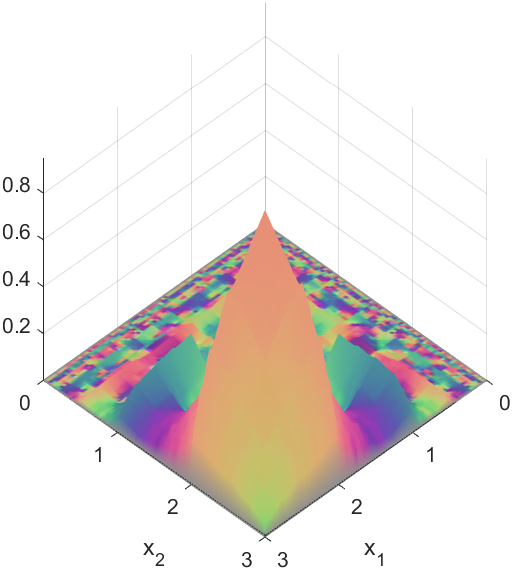
(a) Quaternion-valued scaling function $\varphi$

(b) Quaternion-valued wavelet $\psi_{1}$

(c) Quaternion-valued wavelet $\psi_{2}$

(d) Quaternion-valued wavelet $\psi_{3}$

Figure 1: A wavelet ensemble derived from a solution to Problem 4.1(a) where $\eta=4$ and $\mu=1$. The scaling function $\varphi$ has a measure of separability $\tilde{\zeta}(\varphi)\approx 2.324301$.

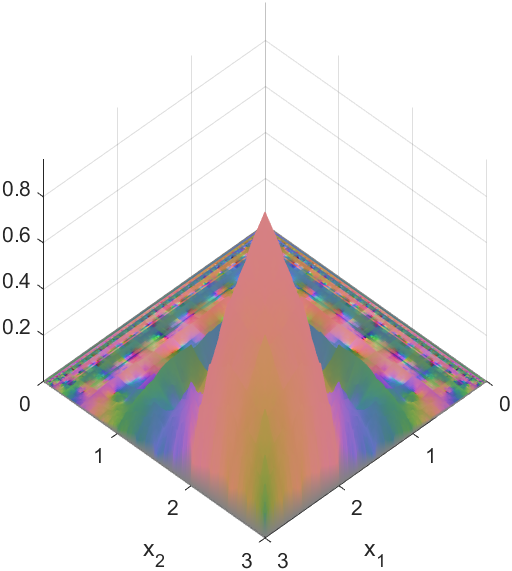
(a) Quaternion-valued scaling function $\varphi$

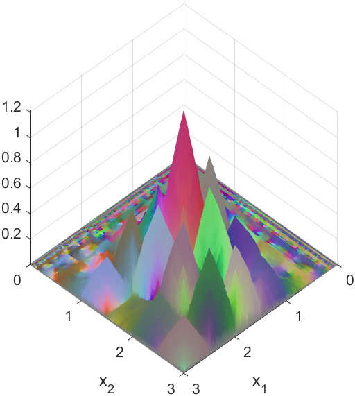
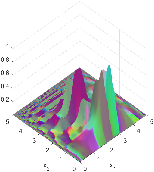
(b) Quaternion-valued wavelet $\psi_{1}$

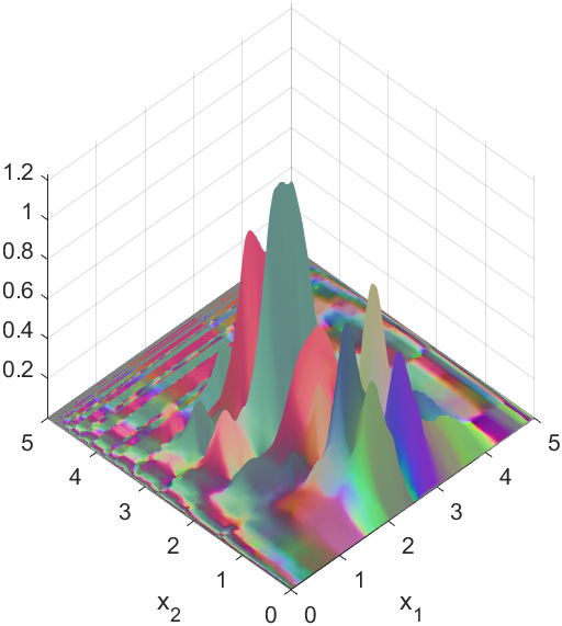
(c) Quaternion-valued wavelet $\psi_{2}$

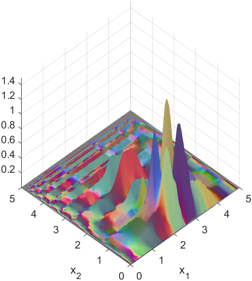
(d) Quaternion-valued wavelet $\psi_{3}$

Figure 2: Another ensemble derived from a solution to Problem 4.1(a) where $\eta=4$ and $\mu=1$. The scaling function $\varphi$ has a measure of separability $\tilde{\zeta}(\varphi)\approx 2.545330$.

(a) Quaternion-valued scaling function $\varphi$

(b) Quaternion-valued wavelet $\psi_{1}$

(c) Quaternion-valued wavelet $\psi_{2}$

(d) Quaternion-valued wavelet $\psi_{3}$

Figure 3: A wavelet ensemble derived from a solution to Problem 4.1(a) where $\eta=6$ and $\mu=2$. The scaling function $\varphi$ has a measure of separability $\tilde{\zeta}(\varphi)\approx 0.592194$.

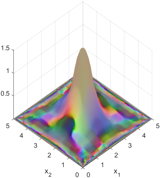
(a) Quaternion-valued scaling function $\varphi$

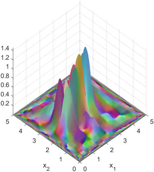
(b) Quaternion-valued wavelet $\psi_{1}$

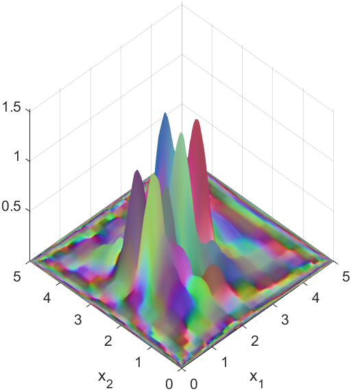
(c) Quaternion-valued wavelet $\psi_{2}$

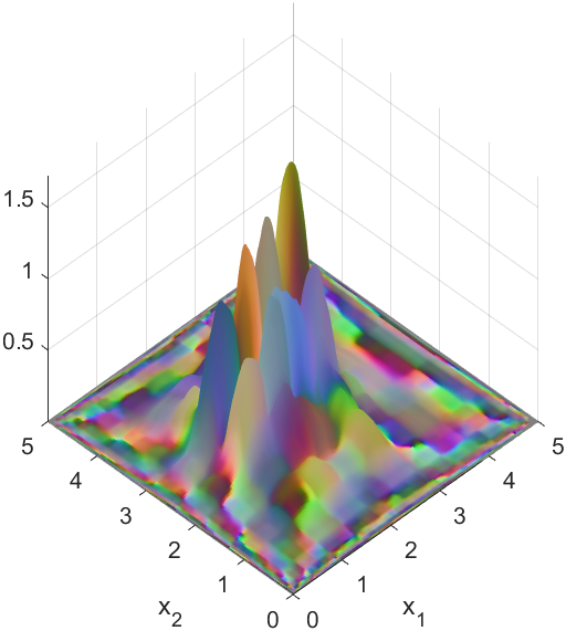
(d) Quaternion-valued wavelet $\psi_{3}$

Figure 4: Another wavelet ensemble derived from a solution to Problem 4.1(a) where $\eta=6$ and $\mu=2$. The scaling function $\varphi$ has a measure of separability $\tilde{\zeta}(\varphi)\approx 1.676368$.

(a) Quaternion-valued scaling function $\varphi$

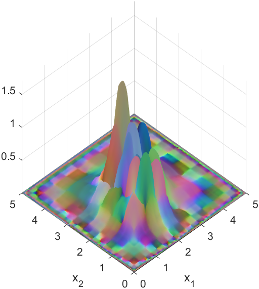
(b) Quaternion-valued wavelet $\psi_{1}$

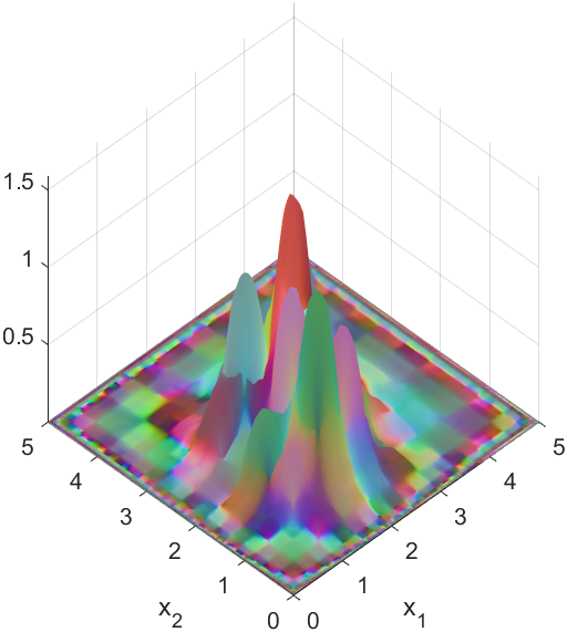
(c) Quaternion-valued wavelet $\psi_{2}$

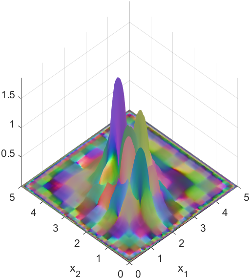
(d) Quaternion-valued wavelet $\psi_{3}$

Figure 5: A wavelet ensemble derived from a solution to Problem 4.1(b) where $\eta=6$ and $\mu=2$. The scaling function $\varphi$ has a measure of separability $\tilde{\zeta}(\varphi)\approx 1.455653$.

(a) Quaternion-valued scaling function $\varphi$

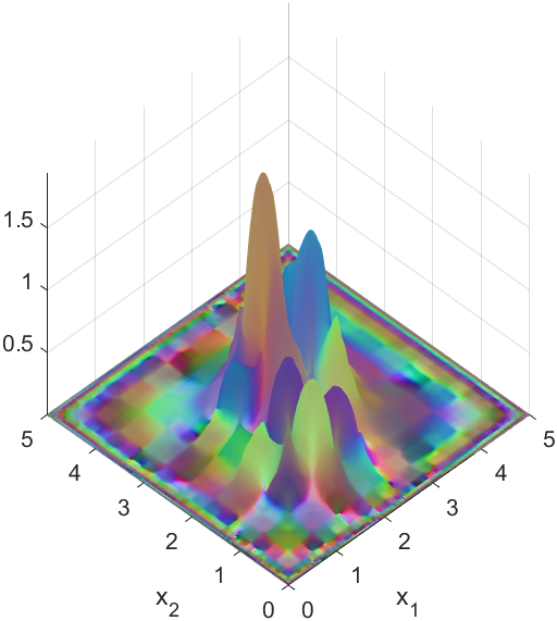
(b) Quaternion-valued wavelet $\psi_{1}$

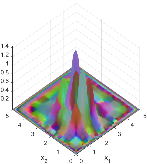
(c) Quaternion-valued wavelet $\psi_{2}$

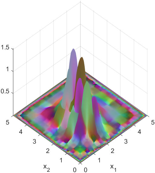
(d) Quaternion-valued wavelet $\psi_{3}$

Figure 6: Another wavelet ensemble derived from a solution to Problem 4.1(b) where $\eta=6$ and $\mu=2$. The scaling function $\varphi$ has a measure of separability $\tilde{\zeta}(\varphi)\approx 0.465628$.

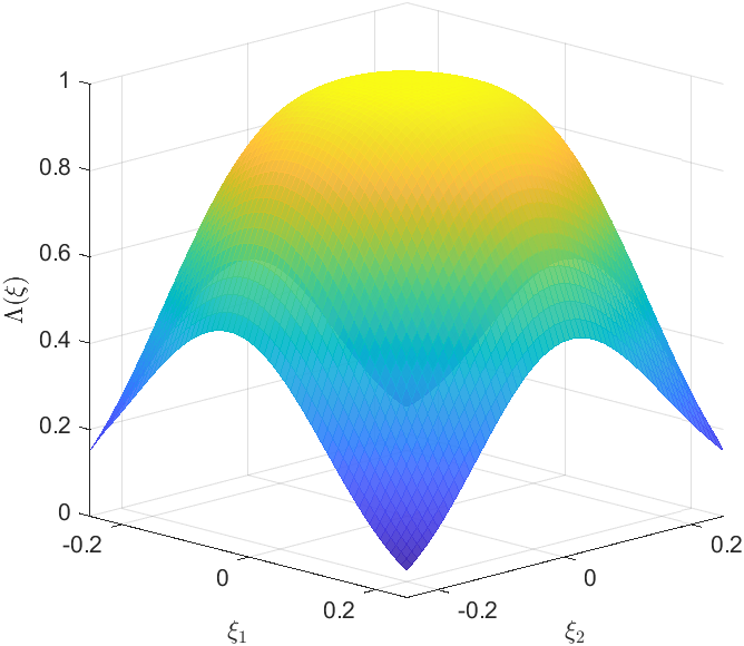
(a) For $\varphi$ in Figure 1

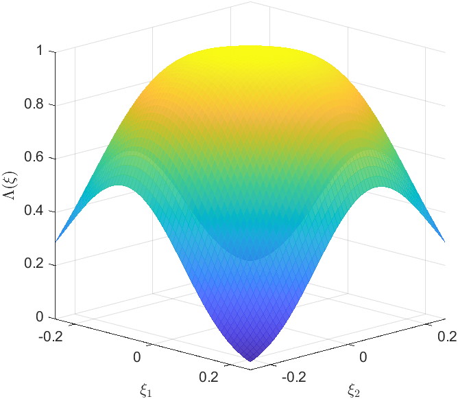
(b) For $\varphi$ in Figure 2

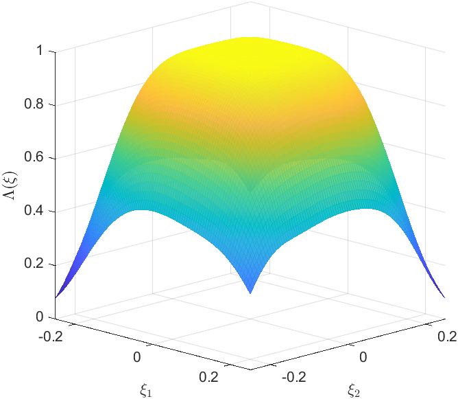
(c) For $\varphi$ in Figure 3

(d) For $\varphi$ in Figure 4

(e) For $\varphi$ in Figure 5

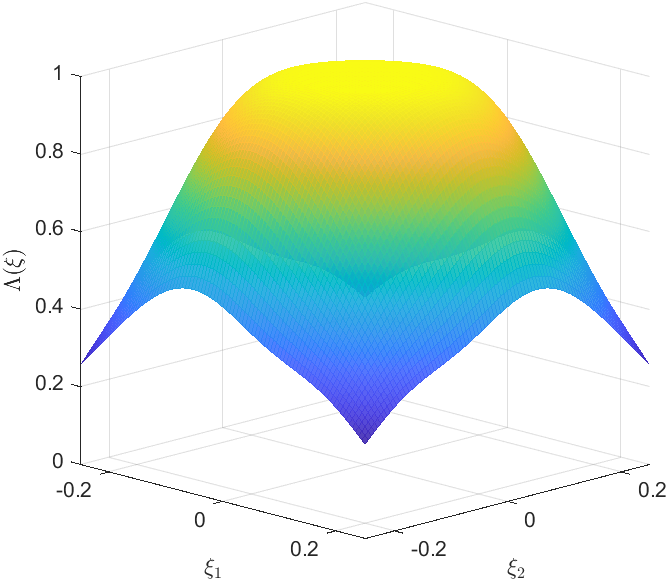
(f) For $\varphi$ in Figure 6

Figure 7: Orthonormality checks for wavelet ensemble solutions.

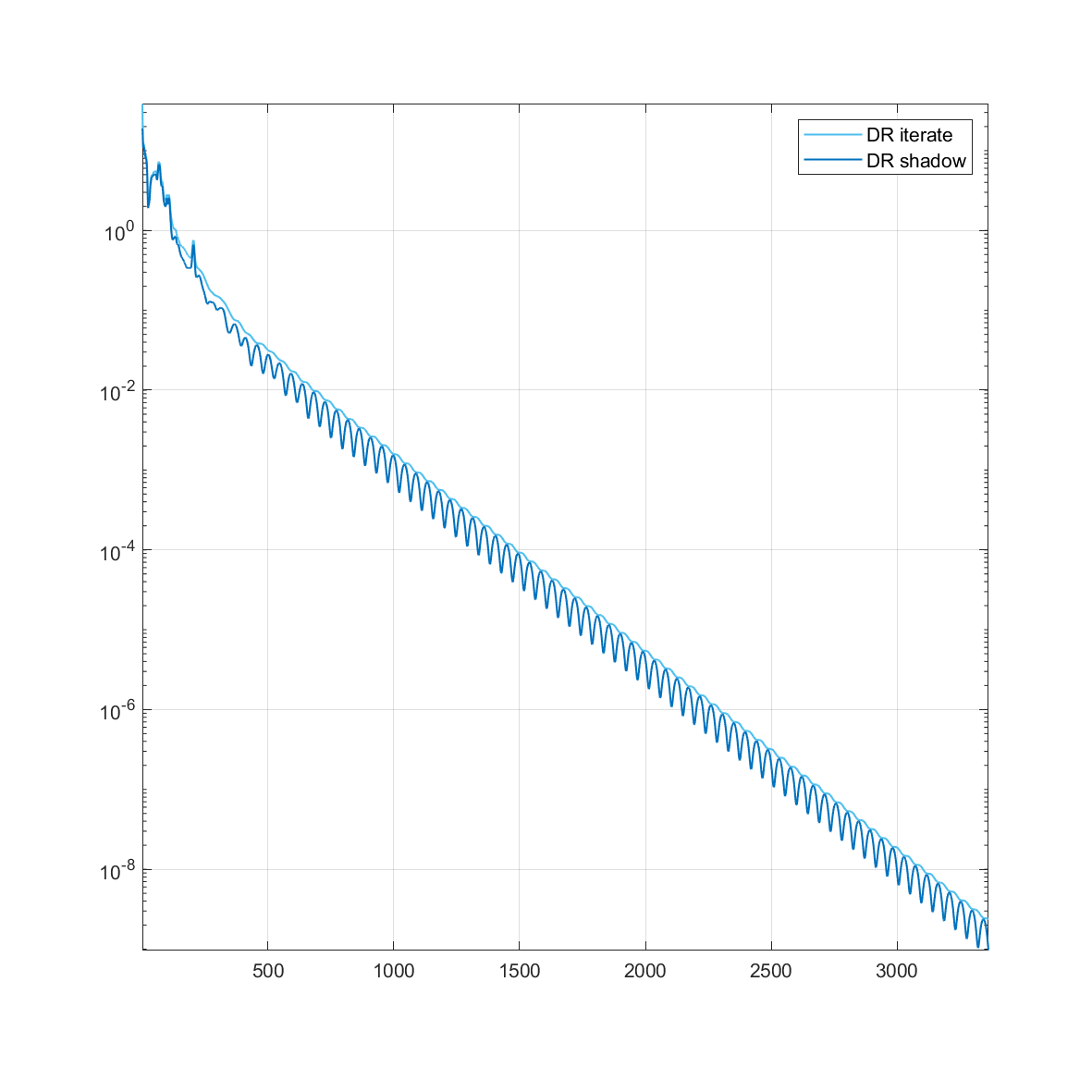
(a) For the wavelet ensemble in Figure 1

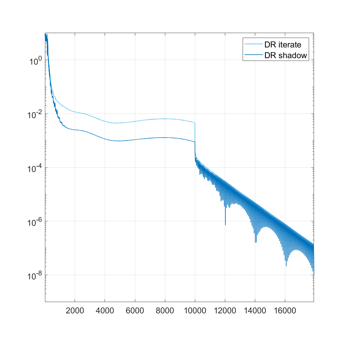
(b) For the wavelet ensemble in Figure 2

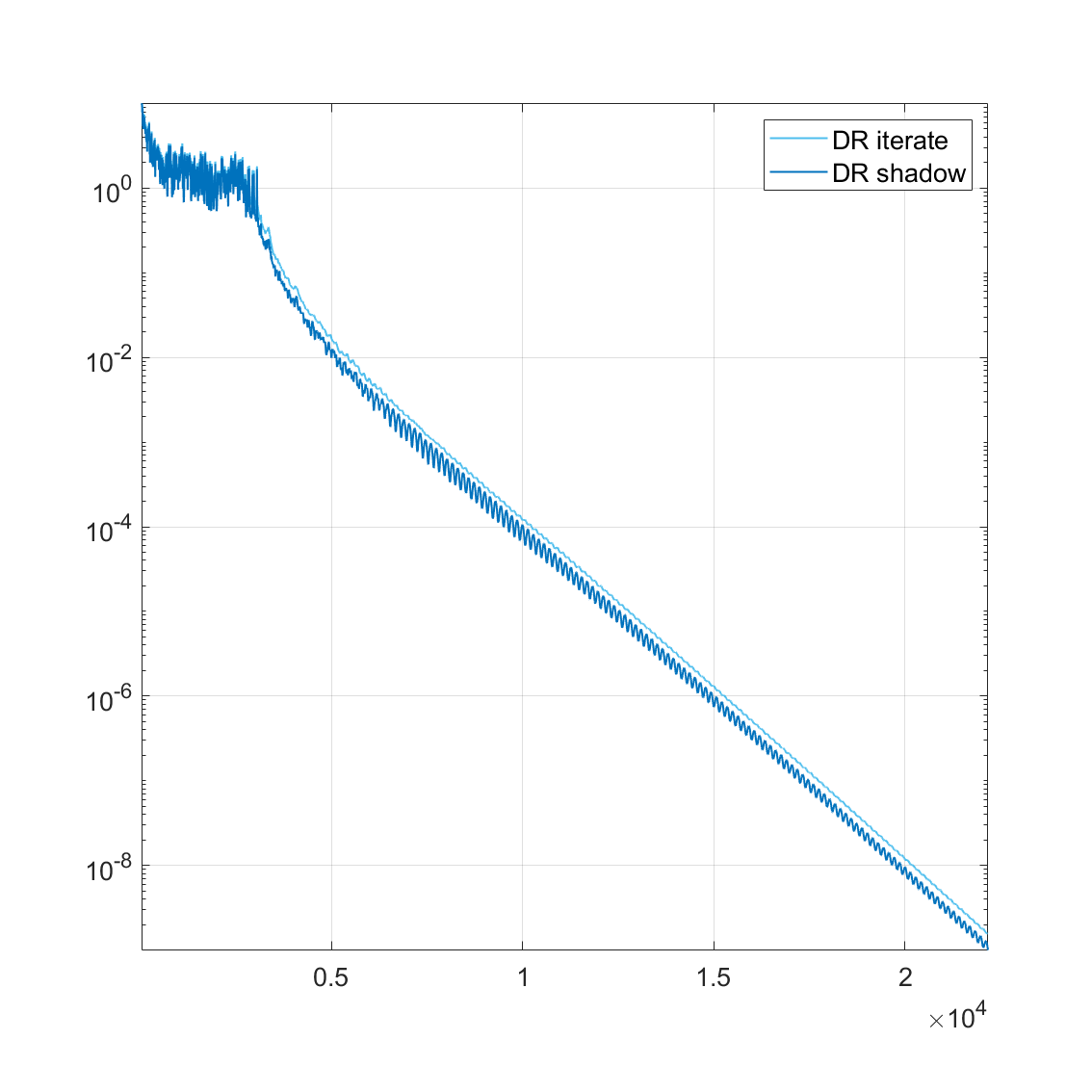
(c) For the wavelet ensemble in Figure 3

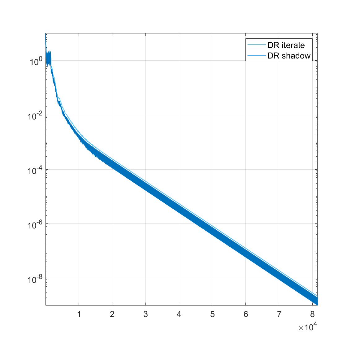
(d) For the wavelet ensemble in Figure 5

Figure 8: Convergence heuristics of DR for selected cases of Problem 4.1.

6 Conclusion

The feasibility approach to wavelet construction served as an alternative method for building classical and higher-dimensional wavelets. It presented a path towards the construction of quaternionic wavelets on the plane. The successful architecture of compactly supported, smooth and orthonormal quaternion-valued wavelets on the plane leaves open many important avenues of research. With these wavelets, the pixel components of a colour image may now be encoded into quaternions for holistic processing of signals using wavelet transforms. With such an approach, the potentially useful correlations between the pixel components are not lost. On this account, developing the mathematics for quaternion-valued wavelet decomposition and reconstruction of colour images poses a possible research direction. It also gives rise to significant research questions about how these quaternion-valued wavelets would perform to image segmentation, denoising and compression when applied to colour images. Cardinality and other types of symmetries may also be added in the design criteria for building quaternionic wavelets.

References

• [1] H. Alfred, Zur theorie der orthogonalen funktionensysteme, Math. Ann., 69 (1910), pp. 331–371.
• [2] F. J. Aragón Artacho, J. M. Borwein, and M. K. Tam, Douglas–Rachford feasibility methods for matrix completion problems, ANZIAM J., 55 (2014), pp. 299–326.
• [3]  , Recent results on Douglas–Rachford methods for combinatorial optimization problems, J. Optim. Theory App., 163 (2014), pp. 1–30.
• [4] F. J. Aragón Artacho, R. Campoy, and M. K. Tam, The Douglas–Rachford algorithm for convex and nonconvex feasibility problems, Math. Method Oper. Res., (2019), pp. 1–40.
• [5] H. H. Bauschke and P. L. Combettes, Convex Analysis and Monotone Operator Theory in Hilbert Spaces, Springer, Cham, 2017.
• [6] H. H. Bauschke and M. N. Dao, On the finite convergence of the Douglas–Rachford algorithm for solving (not necessarily convex) feasibility problems in Euclidean spaces, SIAM J. Optim., 27 (2017), pp. 507–537.
• [7] J. M. Borwein and B. Sims, The Douglas–Rachford algorithm in the absence of convexity, in Fixed-point Algorithms for Inverse Problems in Science and Engineering, Springer, New York, 2011, pp. 93–109.
• [8] J. M. Borwein and M. K. Tam, Reflection methods for inverse problems with applications to protein conformation determination, in Generalized Nash Equilibrium Problems, Bilevel Programming and MPEC, Springer, 2017, pp. 83–100.
• [9] A. Calderón, Intermediate spaces and interpolation, the complex method, Stud. Math., 24 (1964), pp. 113–190.
• [10] A. Cegielski, Iterative Methods for Fixed Point Problems in Hilbert Spaces, vol. 2057, Springer, 2012.
• [11] M. N. Dao and M. K. Tam, A Lyapunov-type approach to convergence of the Douglas–Rachford algorithm for a nonconvex setting, J. Global Optim., 73 (2019), pp. 83–112.
• [12] I. Daubechies, Orthonormal bases of compactly supported wavelets, Commun. Pure Appl. Math., 41 (1988), pp. 909–996.
• [13] I. Daubechies, Ten Lectures on Wavelets, SIAM, Philadelphia, Pennsylvania, 1992.
• [14] N. Dizon, J. Hogan, and S. B. Lindstrom, Circumcentering reflection methods for nonconvex feasibility problems, arXiv preprint arXiv:1910.04384, (2019).
• [15] N. D. Dizon, Optimization in the Construction of Multidimensional Wavelets, PhD thesis, University of Newcastle, 2021.
• [16] N. D. Dizon, J. A. Hogan, and J. D. Lakey, Optimization in the construction of nearly cardinal and nearly symmetric wavelets, in 2019 13th International Conference on Sampling Theory and Applications (SampTA), IEEE, 2019, pp. 1–4.
• [17]  , Optimization in the construction of nearly cardinal and nearly symmetric wavelets, Int. J. Wavelets Multiresolution Inf. Process. (under review), (2021).
• [18] N. D. Dizon, J. A. Hogan, and S. B. Lindstrom, Centering projection methods for wavelet feasibility problems, in Current Trends in Analysis, its Applications and Computation: Proceedings of the 12th ISAAC Congress (forthcoming), Birkhäuser, 2020.
• [19]  , Circumcentered reflections method for wavelet feasibility problems, in Proceedings of the 20th Biennial Computational Techniques and Applications Conference (forthcoming), 2021.
• [20] J. Douglas and H. Rachford, On the numerical solution of heat conduction problems in two and three space variables, Trans. Am. Math. Soc., 82 (1956), pp. 421–439.
• [21] P. Fletcher, Discrete wavelets with quaternion and clifford coefficients, Adv. Appl. Clifford Algebras, 28 (2018), pp. 1–30.
• [22] P. Fletcher and S. J. Sangwine, The development of the quaternion wavelet transform, Signal Process., 136 (2017), pp. 2–15.
• [23] D. Franklin, J. A. Hogan, and M. Tam, Higher-dimensional wavelets and the Douglas–Rachford algorithm, in 2019 13th International Conference on Sampling Theory and Applications (SampTA), IEEE, 2019, pp. 1–4.
• [24] D. Franklin, J. A. Hogan, and M. K. Tam, A Douglas–Rachford construction of non-separable continuous compactly supported multidimensional wavelets, arXiv preprint arXiv:2006.03302, (2020).
• [25] D. J. Franklin, Projection algorithms for non-separable wavelets and Clifford Fourier analysis, PhD thesis, University of Newcastle, 2018.
• [26] P. Ginzberg and A. T. Walden, Matrix-valued and quaternion wavelets, IEEE transactions on signal processing, 61 (2012), pp. 1357–1367.
• [27] A. Grossmann and J. Morlet, Decomposition of Hardy functions into square integrable wavelets of constant shape, SIAM J. Math. Anal., 15 (1984), pp. 723–736.
• [28] W. R. Hamilton, Lectures on Quaternions: Containing a Systematic Statement of a New Mathematical Method; of which the Principles Were Communicated in 1843 to the Royal Irish Academy; and which Has Since Formed the Subject of Successive Courses of Lectures, Delivered in 1848 and Sub Sequent Years, in the Halls of Trinity College, Dublin: With Numerous Illustrative Diagrams, and with Some Geometrical and Physical Applications, University Press by MH, 1853.
• [29] J. Hogan and A. J. Morris, Quaternionic wavelets, Numer. Funct. Anal. Optim., 33 (2012), pp. 1031–1062.
• [30] J. Hogan, A. J. Morris, et al., Translation-invariant Clifford operators, in AMSI International Conference on Harmonic Analysis and Applications, Centre for Mathematics and its Applications, Mathematical Sciences Institute, 2013, pp. 48–62.
• [31] A. Krivoshein, V. Protasov, and M. A. Skopina, Multivariate Wavelet Frames, Springer, 2016.
• [32] P. Lions and B. Merceir, Splitting algorithms for the sum of two nonlinear operators, SIAM J. Numer. Anal., 16 (1979), pp. 964–979.
• [33] S. G. Mallat, Multiresolution approximations and wavelet orthonormal bases of ${L}_{2}(\mathbb{R})$, Trans. Am. Math. Soc., 315 (1989), pp. 69–87.
• [34] Y. Meyer, Orthonormal wavelets, in Wavelets, Springer, 1989, pp. 21–37.
• [35] A. J. Morris, Fourier and Wavelet Analysis of Clifford-Valued Functions, PhD thesis, University of Newcastle, Australia, Callaghan, NSW, 2308, Australia, 2014.
• [36] S.-C. Pei and C.-M. Cheng, A novel block truncation coding of color images using a quaternion-moment-preserving principle, IEEE Trans. Commun., 45 (1997), pp. 583–595.
• [37] G. Pierra, Decomposition through formalization in a product space, Math. Program., 28 (1984), pp. 96–115.
• [38] S. J. Sangwine, Fourier transforms of colour images using quaternion or hypercomplex numbers, Electron. Lett., 32 (1996), pp. 1979–1980.
• [39] S. J. Sangwine and N. L. Bihan, Quaternion toolbox for MATLAB®, 2013 (First public release 2005). http://qtfm.sourceforge.net/.
• [40] B. F. Svaiter, On weak convergence of the Douglas–Rachford method, SIAM J. Control Optim., 49 (2011), pp. 280–287.