Fast Heavy Inner Product Identification Between Weights and Inputs in Neural Network Training

Abstract

In this paper, we consider a heavy inner product identification problem, which generalizes the Light Bulb problem ([1]): Given two sets $A\subset\{-1,+1\}^{d}$ and $B\subset\{-1,+1\}^{d}$ with $|A|=|B|=n$, if there are exact $k$ pairs whose inner product passes a certain threshold, i.e., $\{(a_{1},b_{1}),\cdots,(a_{k},b_{k})\}\subset A\times B$ such that $\forall i\in[k],\langle a_{i},b_{i}\rangle\geq\rho\cdot d$, for a threshold $\rho\in(0,1)$, the goal is to identify those $k$ heavy inner products. We provide an algorithm that runs in $O(n^{2\omega/3+o(1)})$ time to find the $k$ inner product pairs that surpass $\rho\cdot d$ threshold with high probability, where $\omega$ is the current matrix multiplication exponent. By solving this problem, our method speed up the training of neural networks with ReLU activation function.

I Introduction

Efficiently finding heavy inner product has been shown useful in many fundamental optimization tasks such as sparsification [2], linear program with small tree width [3, 4], frank-wolf [5], reinforcement learning [6]. In this paper, we define and study the heavy inner product identification problem, and provide both a randomized and a deterministic algorithmic solution for this problem.

Mathematically, we define our main problem as follows:

Definition I.1 (Heavy inner product between two sets).

Given two sets $A\subset\{-1,+1\}^{d}$ and $B\subset\{-1,+1\}^{d}$ with $|A|=|B|=n$, which are all independently and uniformly random except for $k$ vector pairs $\{(a_{1},b_{1}),\cdots,(a_{k},b_{k})\}\subset A\times B$ such that $\forall i\in[k],\langle a_{i},b_{i}\rangle\geq\rho\cdot d$ for some $0<\rho\leq 1$. The goal is to find these $k$ correlated pairs.

We give an example of this problem in Figure 1. A naive solution to this problem would be, to do a linear scan on every $(a,b)$ pair, which runs in $O(n^{2}d)$ time. In practice, usually $k$ is sufficiently small, so that a $o(n^{2}d)$ algorithm might be possible. This motivates the following question:

Can we design an efficient algorithm to identify the heavy inner product pair $(a,b)\in A\times B$, i.e. runs in $o(n^{2}d)$ time.

We provide a positive answer (Theorem I.2) for the above question by an algorithmic solution (Algorithm 2) . In the algorithm, we use two pairwise independent hash functions to partition $A$ and $B$ into $h=n^{2/3}$ groups of size $n^{1/3}$ as $A_{1},\cdots,A_{h}$ and $B_{1},\cdots,B_{h}$, respectively. After that, we compute a score $C_{i,j}$ for each group pair $A_{i}$ and $B_{j}$ to help identify whether the group pair contains the correlated vector pair with constant success probability. After repeating the process for $O(\log n)$ times, we can locate the target group pairs with polynomially low error

and brute force search within group pairs to find the exact heavy inner product vector pairs. We further accelerate the computation of $C_{i,j}$ by carefully designing matrix multiplication.

I-A Our results

We state our main results in the following theorem:

Theorem I.2 (Our results, informal version of Theorem IV.1).

For the heavy inner product identification problem defined in Def. I.1, there is a constant $c_{0}>0$ such that for correlation $\rho$, we can find the heavy $k$ pairs $\{(a_{1},b_{1}),\cdots,(a_{k},b_{k})\}$ in randomized time $O(n^{2\omega/3+o(1)})$ whenever $d\leq c_{0}\log n$ with probability at least $1-1/n^{10}-k^{2}/n^{2/3}$.

For the current fast matrix multiplication algorithm with $\omega\approx 2.373$ ([7]), our running time becomes $O(n^{1.582})$.

I-B Technique Overview

We briefly present our techniques in designing the algorithm: (1) Setting a high probability threshold for the uncorrelated inner product pairs. (2) Partition $A$ and $B$ into $h=n^{2/3}$ groups respectively and locate the group pair $(i,j)$ with the heavy inner product pair by a score $C_{i,j}$ (3) Accelerate the computation of score function $C_{i,j}$.

Set the high probability threshold.

By picking a threshold $v:=\delta(w/\kappa)\log n$, for large enough $\delta$, constant $w$ and for fixed $\kappa$, we have that for each uncorrelated pair $(x,y)\in A\times B$, $|\langle x,y\rangle|<v$ with probability at least $1-1/n^{13}$. By a union bound over all possible $O(n^{2})$ pairs, we have $|\langle x,y\rangle|<v$ for all such $x,y$ with probability at least $1-1/n^{11}$. Let $\widetilde{x}\in A,\widetilde{y}\in B$ denote the correlated pairs which satisfy that $\langle\widetilde{x},\widetilde{y}\rangle\geq\rho d=v$.

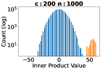
(a)

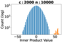
(b)

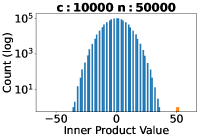
(c)

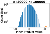
(d)

Figure 1: Simulation for the heavy inner product identification problem , where the $y$ values are in logarithmic scale. For each subfigure, we generated two sets $A\subset\{-1,+1\}^{60}$ and $B\subset\{-1,+1\}^{60}$ with $|A|=|B|=n$, where $c$ pairs of them are correlated and others are randomized. The values of $c,n$ are defined in the subfigures. For each entry in the correlated vector pairs, they have $96\%$ chance to be the same and $4\%$ chance to be different. For uncorrelated vectors, we randomize all of them. We randomly pick a pair $(a,b)$ from $A\times B$ and calculate $\langle a,b\rangle$. We repeat this process $1,000,000$ times and get this histogram. We can clearly see that the inner product of uncorrelated vectors (blue) are distributed around $0$, and their absolute value almost don’t exceed $50$, which is smaller than the dimension of the vector. Additionally, the inner product of correlated vectors (orange) are distributed around $50$. Our goal is to find these correlated vectors.

Locate the group index containing the correlated vector pairs with $C_{i,j}$.

We first partition $A$ and $B$ into $h:=n^{2/3}$ groups and each group contains $g:=n^{1/3}$ elements. For each $x\in A$, we pick a random value $a^{x}\in\{-1,1\}$ independently and uniformly, and for a constant $\tau>0$ define $r:=\lceil\log_{w}(\tau n^{1/3})\rceil$. We define a polynomial $p:\mathbb{R}^{d}\rightarrow\mathbb{R}$ by:

$$p(z_{1},\ldots,z_{d})=(z_{1}+\cdots+z_{d})^{r}.$$

For each group pair $(i,j)$ we compute a score $C_{i,j}$ defined as:

$$C_{i,j}:=\sum_{x\in A_{i}}\sum_{y\in B_{j}}a^{x}\cdot a^{y}\cdot p(x_{1}y_{1},\ldots,x_{d}y_{d}).$$

If the correlated pair is not in $A_{i}\in\{-1,1\}^{d}$ or $B_{j}\in\{-1,1\}^{d}$, $C_{i,j}$ has expectation $0$. For sufficiently large constant $\tau$, by the Chebyshev inequality, we have that

$$|C_{i,j}|\leq\tau n^{1/3}v^{r}/3$$

with probability at least $3/4$. Let $\theta=\tau n^{1/3}v^{r}/3$.

If we repeat the process of selecting the $a^{x}$ values for each $x\in A$ independently at random $O(\log n)$ times, whichever top $k$ group pairs $A_{i},B_{j}$ has $|C_{i,j}|\geq 2\theta$ most frequently will be the pairs containing the heavy inner product vector pairs with high probability. After identifying the group pairs which contain the heavy inner product vector pairs, it remains a brute force search between $k$ pairs of groups, each containing $O(n^{1/3})$ vectors to output the result.

Figure 2: Example of $M_{1},\cdots,M_{t}$, given $d=5$ and $r=2$. In this case, $t=16$ as there are $\sum_{i=0}^{2}\tbinom{5}{i}=16$ distinct subsets $M\subset[d]$ of size less than $2$.

Accelerate computing $C_{i,j}$.

Given $t=\sum_{i=0}^{r}\tbinom{d}{i}$, let $M_{1},\ldots,M_{t}$ be an enumeration of all distinct subsets of $[d]$ of size at most $r$ , we can reorganize $C_{i,j}$ as

$$C_{i,j}= ~{}\sum_{s=1}^{t}(c_{s}\cdot(\sum_{x\in A_{i}}a^{x}\cdot x_{M_{s}})\cdot(\sum_{y\in B_{j}}a^{y}\cdot y_{M_{s}}))$$

for some $c_{s},s\in[t]$ that can be computed in $\operatorname{poly}(r)=\operatorname{poly}\log(n)$ time, where $x_{M}:=\Pi_{i\in M}x_{i}$ for any $M\subseteq[d]$.

And define the matrices $U,V\in\mathbb{Z}^{h\times t}$ by

$$U_{i,s}:=\sum_{x\in A_{i}}a^{x}\cdot x_{M_{s}}\mathrm{~{}~{}and~{}~{}}V_{i,s}:=c_{s}\cdot U_{i,s}.$$

Then we know that the matrix product $C:=UV^{\top}\in\mathbb{Z}^{h\times h}$ is exactly the matrix of the values $C_{i,j}$ we desire and the time complexity of computing the matrix multiplication is

$${\cal T}_{\mathrm{mat}}(n^{2/3},n^{2/3+o(1)},n^{2/3})=O(n^{2\omega/3+o(1)}).$$

In addition, we further speed up the calculation of matrix $U$ and $V$ as follows: Let $N_{1},\ldots,N_{u}$ be an enumeration of all subsets of $[d]$ of size at most $\lceil r/2\rceil$. For each $i\in[h]$, define the matrices $L^{i},\widetilde{L}^{i}\in\mathbb{Z}^{u\times g}$ by $L_{s,x}^{i}:=x_{N_{s}}$ and $\widetilde{L}_{s,x}^{i}:=a^{x}\cdot x_{N_{s}}$. Then compute the product $P^{i}:=L^{i}\widetilde{L}^{i\top}\in\mathbb{R}^{u\times u}$ and each desired entry $U_{i,s}$ can be found as an entry of the computed matrix $P^{i}$. Computing the entries of the $L^{i}$ matrices naively takes

$$O(h\cdot u\cdot g\cdot r)= ~{}\widetilde{O}(n\cdot u)$$

$$= ~{}\widetilde{O}(n^{4/3+o(1)})$$

time, and computing the $P^{i}\in\mathbb{R}^{u\times u}$ takes time

$$O(h)\cdot{\cal T}_{\mathrm{mat}}(u,g,u)=O(n^{(2+\omega)/3+o(1)}).$$

They are all bounded by $O(n^{2\omega/3+o(1)})$ time.

Roadmap.

We first discuss several related works in Section II. We then introduce several preliminary definitions and lemmas in Section III. We present our randomized algorithm design and its main theorem in Section IV. We further provide a deterministic algorithm for the heavy inner product identification problem in Section V. We conclude our contributions in Section VII.

II Related Work

Correlations on the Euclidean Sphere.

[8] proposed a randomized hashing algorithm which rounds the Euclidean sphere to $\{-1,1\}^{d}$. The hash function chooses a uniformly random hyperplane through the origin, and outputs $1$ or $-1$ depending on which side of the hyperplane a point is on. [9] proposed an efficient algorithm to solve the light bulb problem ([1]) where given $n$ input vectors in $\{-1,1\}^{d}$, which are all independently and uniformly random excepted one correlated pair of vectors with high inner product. Our problem is a generalization of theirs, in that our setting has $k$-correlated pairs, with small $k$.

Learning Sparse Parities with Noise.

The Light Bulb Problem was first presented by [10] as a fundamental illustration of a correlational learning problem. The Light Bulb Problem may be generally viewed as a particular instance of a number of other learning theory issues, such as learning sparse parities with noise, learning sparse juntas with or without noise, and learning sparse DNF [11]. Notably, [11] demonstrated that all of these more complex learning issues can be reduced to the Light Bulb Problem as well, and they provide best Light Bulb Problem algorithms following from the fastest known algorithms by applying this reduction.

Acceleration via high-dimensional search data structure.

Finding points in certain geometric query regions can be done efficiently with the use of high-dimensional search data structures. One popular technique is Locality Sensitive Hashing(LSH) [12], which enables algorithms to find the close points. For example, small $\ell_{2}$ distance [13, 14, 15, 16, 17] or large inner product between a query vector $q\in\mathbb{R}^{d}$ and a dataset $S\subset\mathbb{R}^{d}$ [18, 19, 20]. MONGOOSE [21] can retrieve neurons with maximum inner products via a learnable LSH-based data structure [8] and lazy update framework proposed by [22] in order to achieve forward pass acceleration.

Besides LSH, space partitioning data structures like partition trees [23, 24, 25, 26], $k$-$d$ trees [27, 28] can also be leveraged to search the regions.

Sketching

Sketching is a well-known technique to improve performance or memory complexity [29]. It has wide applications in linear algebra, such as linear regression and low-rank approximation [29, 30, 31, 32, 33, 34, 35, 36, 37, 38, 39, 40], training over-parameterized neural network [41, 42, 43], empirical risk minimization [44, 45], linear programming [44, 46, 47, 48, 3, 4], distributed problems [49, 50, 51], clustering [52], generative adversarial networks [53], kernel density estimation [54], tensor decomposition [55, 56], trace estimation [57], projected gradient descent [58, 5], matrix sensing [59, 60], softmax regression and computation [61, 62, 63, 64, 65, 66, 67, 68, 69, 70, 71], John Ellipsoid computation [72, 73], semi-definite programming [4], kernel methods [74, 75, 76, 77, 61, 67, 39], adversarial training [78], cutting plane method [79, 80], discrepancy [81], federated learning [82, 83], kronecker projection maintenance [84], reinforcement learning [85, 86, 6], relational database [87].

III Preliminary

Notations.

For any natural number $n$, we use $[n]$ to denote the set $\{1,2,\dots,n\}$. We use $A^{\top}$ to denote the transpose of matrix $A$. For a probabilistic event $f(x)$, we define ${\bf 1}\{f(x)\}$ such that ${\bf 1}\{f(x)\}=1$ if $f(x)$ holds and ${\bf 1}\{f(x)\}=0$ otherwise. We use $\Pr[\cdot]$ to denote the probability, and use $\operatorname*{{\mathbb{E}}}[\cdot]$ to denote the expectation if it exists. For a matrix $A$, we use $\operatorname{tr}[A]$ for trace of $A$. We use ${\cal T}_{\mathrm{mat}}(a,b,c)$ to denote the time of multiplying an $a\times b$ matrix with another $b\times c$ matrix. For a vector $x\in\{-1,1\}^{d}$, we will use $x_{i}$ to denote the $i$-th entry of $x$ for any $i\in[d]$, and $x_{M}:=\Pi_{i\in M}x_{i}$ for any $M\subseteq[d]$. For two sets $A$ and $B$, we use $A\oplus B$ to denote the symmetric difference of $A$ and $B$.

We give the fast matrix multiplication time notation in the following definition.

Definition III.1 (Matrix Multiplication).

We use ${\cal T}_{\mathrm{mat}}(a,b,c)$ to denote the time of multiplying an $a\times b$ matrix with another $b\times c$ matrix. We use $\omega$ to denote the number such that ${\cal T}_{\mathrm{mat}}(n,n,n)=n^{\omega}$. Usually $\omega$ is called the exponent of matrix multiplication. Currently, $\omega\approx 2.373$ [88, 89].

We will use Hoeffding bound and the Chebyshev’s inequality as a probability tool.

Lemma III.2 (Hoeffding bound [90]).

Let $X_{1},\cdots,X_{n}$ denote $n$ independent bounded variables in $[a_{i},b_{i}].$ Let $X=\sum_{i=1}^{n}X_{i}$, then we have

$$\Pr[|X-\mathbb{E}[X]|\geq t]\leq 2\exp(-\frac{2t^{2}}{\sum_{i=1}^{n}(b_{i}-a_{i})^{2}})$$

Lemma III.3 (Chebyshev’s inequality).

Let $X$ be a random variable with expectation $\mu$ and standard deviation $\sigma$. Then for all $c>0$, we have:

$$\Pr[|X-\mu|\geq c\sigma]\leq\frac{1}{c^{2}}$$

Next, we present the definition of hash function here. Usually, hashing is used in data structures for storing and retrieving data quickly with high probability.

Definition III.4 (Hash function).

A hash function is any function that projects a value from a set of arbitrary size to a value from a set of a fixed size. Let $U$ be the source set and $D$ be the target set, we can define the hash function $h$ as: $h:U\to D$

We will need partition the input sets $A\subset\{-1,1\}^{d}$ and $B\subset\{-1,1\}^{d}$ into groups using the pairwise independent hashing function. The following definition shows the collision probability of pairwise independent hash functions.

Definition III.5 (Pairwise independence).

A family $\mathcal{H}=\{h:U\rightarrow R\}$ is said to be pairwise independent if for any two distinct elements $x_{1}\neq x_{2}\in U$, and any two (possibly equal) values $y_{1},y_{2}\in R$ such that:

$$\Pr_{h\in\mathcal{H}}[h(x_{1})=y_{1}\mathrm{~{}~{}and~{}~{}}h(x_{2})=y_{2}]=\frac{1}{|R|^{2}}$$

where $R$ is a set with finite elements.

IV Algorithm for large inner product between two sets

Roadmap.

In this section, we first present our main result (Theorem IV.1) for the problem defined in Definition I.1 and its corresponding algorithm implementation in Algorithm 1 and Algorithm 2. In Section IV-A we present the correctness lemma and proof for our algorithm. In Section IV-B we present the lemma and proof for our partition based on pairwise independent hash function. We present the time complexity analysis our algorithm in Section IV-C.

Algorithm 1 Algorithm for finding the heavy group pairs and finding the heavy inner product pair within one group pair.

1:data structure

2:members

3:     $\theta\in\mathbb{R}$ $\triangleright$ The threshold for group pair score $C_{i,j}$

4:end members

5:

6:procedure FindHeavyGroupPairs($\{A_{1},\cdots,A_{h}\}\subset\{-1,1\}^{d},\{B_{1},\cdots,B_{h}\}\subset\{-1,1\}^{d},$ $n\in\mathbb{N}_{+},t\in\mathbb{N}_{+}$ )

7:     $R\leftarrow\emptyset$

8:     for $\ell=1\rightarrow 10\log(n)$ do

9:         for $i=1\rightarrow h$ do

10:              for $j=1\rightarrow h$ do $\triangleright$ Pick $a^{x},b^{y}\in\{-1,1\}$ at uniformly random

11:                  $C_{i,j}=\sum_{s=1}^{t}[c_{s}\cdot(\sum_{x\in A_{i}}a^{x}\cdot x_{M_{s}})\cdot(\sum_{y\in B_{j}}a^{y}\cdot y_{M_{s}})]$

12:                  if $C_{i,j}\geq 2\theta$ then

13:                       $R.\textsc{append}((i,j))$

14:                  end if

15:              end for

16:         end for

17:     end for$\triangleright$ $|R|=10k\log(n)$

18:     return $R$

19:end procedure

20:

21:procedure SolveOneGroupPair($A_{i}\subset\{-1,1\}^{d},B_{j}\subset\{-1,1\}^{d},g\in\mathbb{N}_{+}$)

22:     for $q=1\rightarrow g$ do $\triangleright$ Brute force search within each group pair

23:         for $l=1\rightarrow g$ do

24:              if $\langle A_{i,q},B_{j,l}\rangle\geq\rho d$  then

25:                  return $(i\cdot g+q,j\cdot g+l)$ $\triangleright$ Find the heavy inner product vector pair within group $A_{i}$ and $B_{j}$

26:              end if

27:         end for

28:     end for

29:end procedure

30:end data structure

Algorithm 2 Algorithm for heavy inner product between two sets problem.

1:data structure

2:procedure FindCorrelated($A\subset\{-1,1\}^{d},B\subset\{-1,1\}^{d},n\in\mathbb{N}_{+},k\in\mathbb{N}_{+},\tau\in\mathbb{R}_{+},w\in\mathbb{R}_{+},\rho\in(0,1),\delta\in\mathbb{R}$)

3:     Choose two pairwise independent hash functions $h_{A},h_{B}:\{-1,1\}^{d}\rightarrow[n^{2/3}]$

4:     $h\leftarrow n^{2/3},g\leftarrow n^{1/3}$, $v\leftarrow\delta(w/\kappa)\log n$, $r\leftarrow\lceil\log_{w}(\tau n^{1/3})\rceil$, $\theta\leftarrow{\tau n^{1/3}v^{r}}/{3}$

5:     $t\leftarrow\sum_{i=0}^{r}{d\choose i}$

6:     Partition $A$ into $h$ groups $A_{1},\cdots,A_{h}$ and $B$ into $B_{1},\cdots,B_{h}$. Each contains $g$ vectors.

7:     $R\leftarrow\textsc{FindHeavyGroupPairs}(\{A_{1},\cdots,A_{h}\}$,

8:$\{B_{1},\cdots,B_{h}\},n,t)$ $\triangleright$ Time complexity is $O(n^{2\omega/3+o(1)})$, Algorithm 1

9:     $F\leftarrow\emptyset$

10:     for $\ell=1\rightarrow|R|$ do

11:         $(i,j)\leftarrow R_{\ell}$

12:         $p\leftarrow\textsc{SolveOneGroupPair}(A_{i},B_{j},g)$ $\triangleright$ Algorithm 1

13:         $F.\textsc{Append}(p)$

14:     end for

15:     return $F$

16:end procedure

17:end data structure

Theorem IV.1 (Formal version of Theorem I.2).

Given two sets $A\subset\{-1,+1\}^{d}$ and $B\subset\{-1,+1\}^{d}$ with $|A|=|B|=n$, which are all independently and uniformly random except for $k$ vector pairs $\{(a_{1},b_{1}),\cdots,(a_{k},b_{k})\}\subset A\times B$ such that $\forall i\in[k],\langle a_{i},b_{i}\rangle\geq\rho\cdot d$, for some $0<\rho\leq 1$. For every $\epsilon,\rho>0$, there is a $c_{0}>0$ such that for correlation $\rho$, we can find the $k$ pairs $\{(a_{1},b_{1}),\cdots,(a_{k},b_{k})\}$ in randomized time

$$O(n^{2\omega/3+o(1)})$$

whenever $d=c_{0}\log n$ with probability at least $1-1/n^{10}-k^{2}/n^{2/3}$.

Proof.

The correctness of the theorem follows by Lemma IV.2, and the proof of running time follows by Lemma IV.7.

∎

IV-A Correctness of FindCorrelated Algorithm

We first present the following lemma to prove the correctness of FindCorrelated in Algorithm 2 .

Lemma IV.2 (Correctness).

For problem in Defnition I.1, and for every $\epsilon,\rho>0$, there is a $c_{0}>0$ such that for correlation $\rho$ we can find the $k$ pairs $\{(a_{1},b_{1}),\cdots,(a_{k},b_{k})\}$ whenever $d=c_{0}\log n$ with probability at least $1-1/n^{10}-k^{2}/n^{2/3}$.

Proof.

For two constants $\delta,w>0$ to be determined, we will pick $c_{0}=\delta w^{2}/\rho^{2}$. Let $A,B\subset\{-1,1\}^{d}$ be the set of input vectors, and let $\widetilde{x}\in A,\widetilde{y}\in B$ denote the heavy inner product pairs which we are trying to find.

For distinct $x\in A,y\in B$ other than the heavy inner product pairs, the inner product $\langle x,y\rangle$ is a sum of $d$ uniform independent $\{-1,1\}$ values.

Let $v:=\delta(w/\kappa)\log n$. For large enough $\delta$, by a Hoeffding bound stated in Lemma III.2 we have:

$$~{}\Pr[|\langle x,y\rangle-\operatorname*{{\mathbb{E}}}[\langle x,y\rangle]|\geq v]$$

$$= ~{}\Pr[|\langle x,y\rangle|\geq v]$$

$$\leq ~{}2\exp(-\frac{v^{2}}{2n})$$

$$= ~{}2\exp(-\frac{\delta^{2}w^{2}}{2n\kappa^{2}\log^{2}(n)})$$

$$\leq ~{}1/n^{13}$$

where the first step follows that $\operatorname*{{\mathbb{E}}}[\langle x,y\rangle]=0$, the second step follows Hoeffding bound (Lemma III.2), the third step comes from $v=\delta(w/\kappa)\log n$, and the fourth step follows that $\delta^{2}\geq\frac{26n\kappa^{2}\log^{3}(n)}{w^{2}}$. Therefore, we have $|\langle x,y\rangle|<v$ with probability at least $1-1/n^{13}$.

Hence, by a union bound over all $n^{2}-k$ pairs of uncorrelated vectors , we have $|\langle x,y\rangle|<v$ for all such $x,y$ with probability at least $1-1/n^{11}$. We assume henceforth that this is the case. Meanwhile, $\langle\widetilde{x},\widetilde{y}\rangle\geq\rho d=wv$.

Arbitrarily partition $A\subset\{-1,1\}^{d}$ into $h:=n^{2/3}$ groups $A_{1},\ldots,A_{h}\subset\{-1,1\}^{d}$ of size $g:=n/h=n^{1/3}$ per group, and partition $B\subset\{-1,1\}^{d}$ into $h$ groups $B_{1},\ldots,B_{h}\subset\{-1,1\}^{d}$ of size $g$ per group too. According to Lemma IV.3, we condition on that none of the group pair contains more than one heavy inner product vector pair.

For each $x\in A$, our algorithm picks a value $a^{x}\in\{-1,1\}$ independently and uniformly at random. For a constant $\tau>0$ to be determined, let

$$r:=\lceil\log_{w}(\tau n^{1/3})\rceil,$$

and define the polynomial $p:\mathbb{R}^{d}\rightarrow\mathbb{R}$ by

$$p(z_{1},\ldots,z_{d})=(z_{1}+\cdots+z_{d})^{r}.$$

Our goal is, for each $(i,j)\in[h]^{2}$, to compute the value

$$C_{i,j}:=\sum_{x\in A_{i}}\sum_{y\in B_{j}}a^{x}\cdot a^{y}\cdot p(x_{1}y_{1},\ldots,x_{d}y_{d}).$$ (1)

First we explain why computing $C_{i,j}$ is useful in locating the groups which contain the correlated pair.

Denote

$$p(x,y):=p(x_{1}y_{1},\ldots,x_{d}y_{d}).$$

Intuitively, $p(x,y)$ is computing an amplification of $\langle x,y\rangle$. $C_{i,j}$ sums these amplified inner products for all pairs $(x,y)\in A_{i}\times B_{j}$. We can choose our parameters so that the amplified inner product of the correlated pair is large enough to stand out from the sums of inner products of random pairs with high success probability.

Let us be more precise. Recall that for uncorrelated $x,y$ we have $|\langle x,y\rangle|\leq v$, and hence $|p(x,y)|\leq v^{r}$

Similarly, we have

$$|p(\widetilde{x},\widetilde{y})|\geq~{}(wv)^{r}\geq~{}\tau n^{1/3}v^{r}.$$

where the first step comes from $(\widetilde{x},\widetilde{y})$ is the correlated pair , and the second step comes from $r=\lceil\log_{w}(\tau n^{1/3})\rceil$

For $x\in A,y\in B$, define

$$a^{(x,y)}:=a^{x}\cdot a^{y}.$$

Notice that,

$$C_{i,j}=\sum_{x\in A_{i},y\in B_{j}}a^{(x,y)}\cdot p(\langle x,y\rangle),$$

where the $a^{(x,y)}$ are pairwise independent random $\{-1,1\}$ values.

We will now analyze the random variable $C_{i,j}$ where we think of the vectors in $A$ and $B$ as fixed, and only the values $a^{x}$ as random. Consider first when the correlated pair are not in $A_{i}\in\{-1,1\}^{d}$ and $B_{j}\in\{-1,1\}^{d}$. Then, $C_{i,j}$ has mean 0 , and (since variance is additive for pairwise independent variables) $C_{i,j}$ has variance at most

$$|A_{i}|\cdot|B_{j}|\cdot\max_{x\in A_{i},y\in B_{j}}|p(\langle x,y\rangle)|^{2}\leq n^{2/3}\cdot v^{2r}.$$

For a constant $\tau=\sqrt{10}$, we have that

$$\Pr[|C_{i,j}|\leq\tau/3\cdot n^{1/3}v^{r}]\geq~{}\frac{9}{\tau^{2}}=~{}9/10$$

where the first step follows that $C_{i,j}$ has mean $0$, $\sigma=n^{1/3}v^{r}$ and the Chebyshev inequality from Lemma III.3, and the second step comes from $\tau=\sqrt{10}$.

Let $\theta=\tau n^{1/3}v^{r}/3$, so $|C_{i,j}|\leq\theta$ with probability at least $9/10$. Meanwhile, if $\widetilde{x}\in A_{i}$ and $\widetilde{y}\in B_{j}$, then $C_{i,j}$ is the sum of $a^{(\widetilde{x},\widetilde{y})}p(\langle\widetilde{x},\widetilde{y}\rangle)$ and a variable $C^{\prime}$ distributed as $C_{i,j}$ was in the previous paragraph.

Hence, since $|p(\langle\widetilde{x},\widetilde{y}\rangle)|\geq\tau n^{1/3}v^{r}=3\theta$, and $|C^{\prime}|\leq\theta$ with probability at least $9/10$, we get by the triangle inequality that $|C_{i,j}|\geq 2\theta$ with probability at least $9/10$.

Hence, if we repeat the process of selecting the $a^{x}$ values for each $x\in A$ independently at random $10\log n$ times, and check all group pairs $(A_{i},B_{j})$ having $|C_{i,j}|\geq 2\theta$ in a brute force manner to locate the heavy inner product vector pairs. For each group pair brute force check, the time complexity is $O(n^{2/3})$ and there are $10k\log n$ group pairs to check. The failure probability is $1-k/n^{11}$.

In all, by a union bound over all possible errors and the probability that any group pair contains more than one heavy inner product vector pairs from Lemma IV.3, this will succeed with probability at least

$$~{}1-(k+1)/n^{11}-k^{2}/n^{2/3}\geq~{}1-1/n^{10}-k^{2}/n^{2/3}$$

∎

IV-B Partition Collision Probability

In the following lemma, we prove that if there are $k$ heavy inner product vector pairs in $A$ and $B$, the probability of none of the group pair contains more than one heavy inner product vector pair is $1-k^{2}/n^{2/3}$.

Lemma IV.3.

With two pairwise independent hash function $h_{A}$ and $h_{B}$, we partition two sets $A,B\subset\{-1,1\}^{d}$ into $h=n^{2/3}$ groups respectively. Suppose there are $k$ heavy vector inner product pairs $\{(a_{1},b_{1}),\cdots,(a_{k},b_{k})\}\subset A\times B$, the probability where none of the group pair contains more than one heavy inner product vector pair is $1-k^{2}/n^{2/3}$.

Proof.

If any two vector pairs $(a_{x},b_{x}),(a_{y},b_{y})\in\{(a_{1},b_{1}),\cdots,(a_{k},b_{k})\}\subset A\times B$ collide in a group pair $(A_{i},B_{j})$, according to the collision property of hash function $h_{A}$ and $h_{B}$, the probability is ${n^{-2/3}}$. By union bound across all $k^{2}$ possible heavy inner product vector pairs, we know that the probability of none of any two vector pairs in $\{(a_{1},b_{1}),\cdots,(a_{k},b_{k})\}$ collide into the same group is $1-k^{2}/n^{2/3}$.

This completes the proof. ∎

IV-C Running Time of FindCorrelated Algorithm

We split the time complexity of FindCorrelated in Algorithm 2 into two steps and analyze the first step in Lemma IV.4.

IV-C1 Running time of finding heavy group pairs

Lemma IV.4 (Time complexity of FindHeavyGroupPairs).

For every $\epsilon,\rho>0$, FindHeavyGroupPairs in Algorithm 1 for heavy inner product between two sets problem in Definition I.1 of correlation $\rho$ runs in

$$O(n^{2\omega/3+o(1)})$$

time with a $c_{0}>0$ and $d=c_{0}\log n$ to find all the group pairs which contains the heavy inner product vector pairs.

Proof.

Before computing $C_{i,j}$, we will rearrange the expression for $C_{i,j}$ into one which is easier to compute. Since we are only interested in the values of $p$ when its inputs are all in $\{-1,1\}$, we can replace $p$ with its multilinearization $\widehat{p}$.

Let $M_{1},\ldots,M_{t}$ be an enumeration of all subsets of $[d]$ of size at most $r$, thus we know $t$ can be calculated as follows:

$$t=\sum_{i=0}^{r}{d\choose i}.$$

Then, there are coefficients $c_{1},\ldots,c_{t}\in\mathbb{Z}$ such that

$$\widehat{p}(x)=\sum_{s=1}^{t}c_{s}x_{M_{s}}.$$

Rearranging the order of summation of Eq. (1) , we see that we are trying to compute

$$C_{i,j}= ~{}\sum_{s=1}^{t}\sum_{x\in A_{i}}\sum_{y\in B_{j}}a^{x}\cdot a^{y}\cdot c_{s}\cdot x_{M_{s}}\cdot y_{M_{s}}$$

$$= ~{}\sum_{s=1}^{t}(c_{s}\cdot(\sum_{x\in A_{i}}a^{x}\cdot x_{M_{s}})\cdot(\sum_{y\in B_{j}}a^{y}\cdot y_{M_{s}}))$$ (2)

In order to compute $C_{i,j}$, we first need to compute the coefficients $c_{s}$. Notice that $c_{s}$ depends only on $|M_{s}|$ and $r$. We can thus derive a simple combinatorial expression for $c_{s}$, and hence compute all of the $c_{s}$ coefficients in $\operatorname{poly}(r)=\mathrm{polylog}(n)$ time. Alternatively, by starting with the polynomial $(z_{1}+\cdots+z_{d})$ and then repeatedly squaring then multilinearizing, we can easily compute all the coefficients in $O(t^{2}\mathrm{polylog}(n))$ time; this slower approach is still fast enough for our purposes.

Define the matrices $U,V\in\mathbb{Z}^{h\times t}$ by

$$U_{i,s}:=\sum_{x\in A_{i}}a^{x}\cdot x_{M_{s}}\mathrm{~{}~{}and~{}~{}}V_{i,s}:=c_{s}\cdot U_{i,s}.$$

Notice from Eq. (IV-C1) that the matrix product $C:=UV^{\top}\in\mathbb{Z}^{h\times h}$ is exactly the matrix of the values $C_{i,j}$ we desire.

A simple calculation (see Lemma IV.5 below) shows that for any $\epsilon>0$, we can pick a sufficiently big constant $w>0$ such that $t=O(n^{2/3+o(1)})$.

Since $h=O(n^{2/3})$, if we have the matrices $U,V$, then we can compute this matrix product in

$${\cal T}_{\mathrm{mat}}(n^{2/3},n^{2/3+o(1)},n^{2/3})=O(n^{2\omega/3+o(1)})$$

time, completing the algorithm.

Unfortunately, computing the entries of $U$ and $V$ naively would take $\Omega(h\cdot t\cdot g)=\Omega(n^{5/3})$ time, which is slower than we would like.

Let $N_{1},\ldots,N_{u}$ be an enumeration of all subsets of $[d]$ of size at most $\lceil r/2\rceil$. For each $i\in[h]$, define the matrices $L^{i},\widetilde{L}^{i}\in\mathbb{Z}^{u\times g}$ (whose columns are indexed by elements $x\in A_{i}$ ) by

$$L_{s,x}^{i}:=x_{N_{s}}\mathrm{~{}~{}and~{}~{}}\widetilde{L}_{s,x}^{i}:=a^{x}\cdot x_{N_{s}}.$$

Then compute the product $P^{i}:=L^{i}\widetilde{L}^{i\top}\in\mathbb{R}^{u\times u}$. We can see that

$$P_{s,s^{\prime}}^{i}=\sum_{x\in A_{i}}a^{x}\cdot x_{N_{s}\oplus N_{s^{\prime}}},$$

where $N_{s}\oplus N_{s^{\prime}}$ is the symmetric difference of $N_{s}$ and $N_{s^{\prime}}$. Since any set of size at most $r$ can be written as the symmetric difference of two sets of size at most $\lceil r/2\rceil$, each desired entry $U_{i,s}$ can be found as an entry of the computed matrix $P^{i}$. Similar to our bound on $t$ from before (see Lemma IV.5 below), we see that for big enough constant $w$, we have $u=O(n^{1/3+o(1)})$. Computing the entries of the $L^{i}$ matrices naively takes only

$$O(h\cdot u\cdot g\cdot r)=~{} \widetilde{O}(n\cdot u)$$

$$=~{} \widetilde{O}(n^{4/3+o(1)})$$

time, and then computing the products $P^{i}\in\mathbb{R}^{u\times u}$ takes time

$$O(h)\cdot{\cal T}_{\mathrm{mat}}(u,g,u)=O(n^{(2+\omega)/3+o(1)}).$$

Both of these are dominated by $O(n^{2\omega/3+o(1)})$. This completes the proof. ∎

We will need the following lemma to prove the time complexity of our algorithm.

Lemma IV.5.

Let $d=O(w^{2}\log(n))$ and $n=|A|=|B|$ be the vector dimension and number of vectors in Theorem IV.1, and let

$$r:=\lceil\log_{w}(\tau n^{1/3})\rceil,u:={d\choose r/2},t:={d\choose r}$$

For every $\epsilon>0$, and there is a $w>0$ such that we can bound

$$t=O(n^{2/3+o(1)}),u=O(n^{1/3+o(1)}).$$

Lemma IV.5 implies that for any $\epsilon>0$, we can find a sufficiently large $w$ to bound the time needed to compute $UV^{\top}$ and $P^{i}:=L^{i}\widetilde{L}^{i\top}$.

Proof.

Recall that $r=\log_{w}(O(n^{1/3}))$. We can upper bound $t$ as follows:

$$t\leq ~{}(r+1)\cdot{d\choose r}$$

$$\leq ~{}(r+1)\cdot(ed/r)^{r}$$

$$\leq ~{}O(w^{2}\log(w))^{\log_{k}(O(n^{1/3}))}$$

$$= ~{}n^{2/3+O(\log\log(w)/\log(w))}$$

where the first step follows from $t=\sum_{i=0}^{r}{d\choose i}\leq(r+1)\cdot{d\choose r}$, the second step follows that ${d\choose r}\leq(ed/r)^{r}$, the third step comes from the value of $d$ and $r$, and the final step comes from $a^{\log_{a}n}=n$. For any $\epsilon>0$ we can thus pick a sufficiently large $w$ so that $t\leq O(n^{2/3+o(1)})$.

We can similarly upper bound ${d\choose r/2}$ $\leq O(n^{1/3+o(1)})$ which implies our desired bound on $u$.

This completes the proof. ∎

IV-C2 Running time of solving heavy group pairs

Then we analyze the time complexity of solving heavy group pairs in Lemma IV.6.

Lemma IV.6 (Time complexity of solving heavy group pairs ).

For every $k,\rho>0$, solving the heavy group pairs in Algorithm 1 for heavy inner product between two sets problem in Definition I.1 of correlation $\rho$ runs in $\widetilde{O}(k\cdot n^{2/3})$ time.

Proof.

Recall that for finding the heavy group pairs of FindCorrelated algorithm, we use two pairwise independent hash function $h_{A}$ and $h_{B}$ to partition $A$ into $h:=n^{2/3}$ groups $A_{1},\ldots,A_{h}$ of size $g:=n/h=n^{1/3}$ per group, and partition $B$ into $h$ groups $B_{1},\ldots,B_{h}$ of size $g$ per group too.

Because we have found $10k\log n$ group pairs $\{(A_{i,1},B_{j,1}),\cdots,(A_{1,k},B_{j,k})\}$ which contain the $k$ heavy inner product vector pairs at the end of FindHeavyGroupPairs with high probability, a brute force within these group pairs of $O(n^{1/3})$ vectors can find the correlated pair in $\widetilde{O}(k\cdot n^{2/3})$ time. This completes the proof. ∎

IV-C3 Overall running time

With the above two lemmas in hand, we can obtain the overall time complexity of FindCorrelated algorithm in Lemma IV.7.

Lemma IV.7 (Time complexity).

For problem in Definition I.1, and for every $\rho>0$, there is algorithm (Algorithm 2 ) such that for correlation $\rho$ we can find the $k$ pairs $\{(a_{1},b_{1}),\cdots,(a_{k},b_{k})\}$ whenever $d=c_{0}\log n$ in

$$O(n^{2\omega/3+o(1)})$$

time.

Proof.

The proof follows by Lemma IV.4 and Lemma IV.6. We can obtain the overall time complexity by:

$$\mathrm{total~{}time}= ~{}O(n^{2\omega/3+o(1)})+\widetilde{O}(k\cdot n^{2/3})$$

$$= ~{}O(n^{2\omega/3+o(1)})$$

where the first step comes from the time complexity of FindHeavyGroupPairs and solving all heavy group pairs in Lemma IV.4 and Lemma IV.6, and the second step follows that

$$O(n^{2\omega/3+o(1)})>\widetilde{O}(k\cdot n^{2/3}).$$

This completes the proof. ∎

V Deterministic Algorithm

We now present a deterministic algorithm for the heavy inner product between two sets problem. Each is a slight variation on the algorithm from the previous section.

Algorithm 3 Deterministic algorithm for heavy inner product between two sets problem.

1:procedure FindRandomBits($A\subset\{-1,1\}^{d},B\subset\{-1,1\}^{d},\rho\in(0,1),n\in\mathbb{N}_{+}$)

2:     Initialize an empty set $\widetilde{A}$

3:     for $i=1\rightarrow n$ do

4:         $r\leftarrow 0$

5:         for $j=1\rightarrow n$ do

6:              if $\langle a_{i},b_{j}\rangle\geq\rho d$ then

7:                  $r\leftarrow 1$ $\triangleright$ If the inner product of vector $a_{i}$ and $b_{j}$ surpass the threshold, we set $r:=1$.

8:              end if

9:         end for

10:         if $r=0$ then

11:              $\widetilde{A}.\textsc{append}(a_{i})$ $\triangleright$ If $a_{i}$ is a random vector, we include it in the set $\widetilde{A}$.

12:         end if

13:         if $|\widetilde{A}|\geq\log n$ then

14:              Break $\triangleright$ We have collected enough random vector for next step.

15:         end if

16:     end for

17:     return $\widetilde{A}$

18:end procedure

19:procedure FindCorrelated($A\subset\{-1,1\}^{d},B\subset\{-1,1\}^{d},n\in\mathbb{N}_{+},k\in\mathbb{N}_{+},\tau\in\mathbb{R}_{+},w\in\mathbb{R}_{+},\rho\in(0,1),\delta\in\mathbb{R}$ )

20:     Choose two pairwise independent hash functions $h_{A},h_{B}:\{-1,1\}^{d}\rightarrow[n^{2/3}]$

21:     $h\leftarrow n^{2/3},g\leftarrow n^{1/3}$, $v\leftarrow\delta(w/\kappa)\log n$, $r\leftarrow\lceil\log_{w}(\tau n^{1/3})\rceil$, $\theta\leftarrow{\tau n^{1/3}v^{r}}/{3}$

22:     $t\leftarrow\sum_{i=0}^{r}{d\choose i}$

23:     Partition $A$ into $h$ groups $A_{1},\cdots,A_{h}$ and $B$ into $h$ groups $B_{1},\cdots,B_{h}$. Each contains $g$ vectors.

24:     $\widetilde{A}\leftarrow\textsc{FindRandomBits}(A,B,\rho,n)$ $\triangleright$ Time complexity is $O(n\log^{2}(n))$

25:     $R\leftarrow\textsc{FindHeavyGroupPairs}(\{A_{1},\cdots,A_{h}\},$ $\{B_{1},\cdots,B_{h}\},n,t)$

26:     $\triangleright$ Time complexity is $O(n^{2\omega/3+o(1)})$. The $a^{x}$ and $a^{y}$ generation uses the random bits from $\widetilde{A}$. Algorithm 1

27:     $F\leftarrow\emptyset$ $\triangleright$ We use set $F$ to store all correlated vector pairs

28:     for $\ell=1\rightarrow|R|$ do

29:         $(i,j)\leftarrow R_{\ell}$ $\triangleright$ Obtain the group pair index which contains heavy inner product vector pair

30:         $p\leftarrow\textsc{SolveOneGroupPair}(A_{i},B_{j},g)$ $\triangleright$ Algorithm 1

31:         $F.\textsc{Append}(p)$

32:     end for

33:     return $F$

34:end procedure

Lemma V.1.

For every $\rho>0$, there is a $c_{0}>0$ and a deterministic algorithm (FindCorrelated in Algorithm 3 ) such that the heavy inner product between two sets problem in Definition I.1 of correlation $\rho$ can be solved in deterministic time $O(n^{2\omega/3+o(1)})$ on almost all instances whenever $d=c_{0}\log n$.

Proof.

In the randomized algorithm described in Algorithm 1, the only randomness used is the choice of independently and uniformly random $a^{x}\in\{-1,1\}$ for each $x\in A$ and the two pairwise independent hash functions, which requires $\Theta(n)$ random bits.

Because we repeat the entire algorithm $\Theta(\log n)$ times to get the correctness guarantee with high success probability, we need $\Theta(n\log n)$ random bits in total.

By standard constructions, we can use $O(\log n)$ independent random bits to generate $n$ pairwise-independent random bits for the pairwise-independent $a^{x}$ variables. Therefore, we only needs $O(\log^{2}n)$ independent random bits in the FindCorrelated algorithm. We can also use the bits to construct two pairwise independent hash functions used for partitioning the input sets into groups.

Our deterministic algorithm executes as follows:

• Choose the same $c_{0}$ value as in Theorem IV.1.

• Let $A,B\subset\{-1,1\}^{d}$ be the input vectors. Initialize an empty set $\widetilde{A}\subset\{-1,1\}^{d}$.

• For $i=1\rightarrow n$, brute-force test whether $a_{i}$ is correlated with any vector in $B$, where $a_{i}$ is a vector in $A$. If not, we save $a_{i}$ into $\widetilde{A}$ until $|\widetilde{A}|=\Theta(\log n)$. We can assume that the vectors in $\widetilde{A}$ are all uniformly random vectors from $\{-1,1\}^{d}$, because they do not produce heavy inner product with any vector in $B$. This can be done in $O(|\widetilde{A}|\cdot|B|\cdot d)=O(n\log^{2}(n))$ time.

• we can use $\widetilde{A}$ as $d\cdot|\widetilde{A}|=\Theta(\log^{2}n)$ independent uniformly random bits. We thus use them as the required randomness to run the FindCorrelated on input vectors in $A$ and $B$. That algorithm has polynomially low error according to Theorem IV.1.

Because the time spent on checking if a subset $\widetilde{A}$ contains the heavy inner product pair is only $O(n\log^{2}(n))$, and the second part of Algorithm 3 takes $O(n^{2\omega/3+o(1)})$ time according to Theorem IV.1, we have the overall time complexity:

$$~{}O(n\log^{2}(n))+O(n^{2\omega/3+o(1)})=~{}O(n^{2\omega/3+o(1)})$$

This completes the proof.

∎

VI Speedup Neural Networks Training

The training of a neural network usually consists of forward and backward propagation, which includes the computations as a function of the input, the network weights and the activation functions. In practice, not all neurons are activated so we can use shifted ReLU function [41]: $\sigma(x)=\max\{\langle w_{r},x\rangle,b_{r}\}$ to speedup the training. Then it’s possible that there is an algorithm whose running time outperforms the naive “calculate and update” method, by detecting the activated neurons and update accordingly. This setting coincides with heavy inner product identification: We can view the forward propagation of the neural network as 1) identify the heavy inner product, where the goal is to identify the heavy inner product (between input and weight) which surpasses the activation function threshold and activates corresponding neurons. 2) forward the neurons with heavy inner product to the next layer, and update the desired function accordingly.

Definition VI.1 (Two Layer Fully Connected Neural Network).

We will consider two-layer fully connected neural networks with $m$ hidden neurons using shifted ReLU $\sigma:\mathbb{R}\rightarrow\mathbb{R}$ as the activation function. We first define the two-layer shifted ReLU activation neural network$f(x):=\sum_{r=1}^{m}a_{r}\cdot\sigma_{\tau}(\langle w_{r},x\rangle)$ where $\sigma_{\tau}(z)=\max\{z,\tau\}$ is the shifted ReLU activation function, $\{w_{r}\}_{r=1}^{m}\subset\mathbb{R}^{d}$ is the weight vector, $\{a_{r}\}_{r=1}^{m}\subset\mathbb{R}$ is the output weight vector, and $x\in\mathbb{R}^{d}$ is the input vector.

Consider activation threshold $\tau=\rho d$. In each iteration of gradient descent, it is necessary for us to perform prediction computations for each point in the neural network. For each input vector $x_{i}\in\mathbb{R}^{d}$, it needs to compute $m$ inner product in $d$ dimensions. Therefore, $\Theta(mnd)$ time is a natural barrier to identify which weight and input index pairs surpass the shifted ReLU activation function threshold $\tau$ per training iteration.

When the neurons are sparsely activated, such a naive linear scan of the neurons is what we want to avoid. We want to locate the heavy inner product pairs that activate the neurons between the weight vectors $\{w_{r}\}_{r=1}^{m}\subseteq\mathbb{R}^{d}$ and input vectors $\{x_{i}\}_{i=1}^{n}\subseteq\mathbb{R}^{d}$. The methods we proposed in this paper can solve this problem efficiently. For the ReLU, it has been observed that the number of neurons activated by ReLU is small, so our method may potentially speed up optimization for those settings as well.

VII Conclusion

In this paper, we design efficient algorithms to identify heavy inner product between two different sets. Given two sets $A\subset\{-1,+1\}^{d}$ and $B\subset\{-1,+1\}^{d}$ with $|A|=|B|=n$, we promise that we can find $k$ pairs of $(a,b)\in A\times B$ such that all of them satisfy $\langle a,b\rangle\geq\rho\cdot d$, for some constant $\rho$. Both the deterministic and the probabilistic algorithm run in $O(n^{2\omega/3+o(1)})=O(n^{1.582+o(1)})$ time to find all the heavy inner product pairs with high probability. In general, our algorithm will consume energy when running, but the theoretical guarantee helps speedup solving the heavy inner product identification problem. However, there are still some limitations of our works. For example, whether how we calculate the correlation between groups is the most efficient way to the heavy inner product problem. As far as we know, our work does not have any negative societal impact.

References

- [1] R. Paturi, S. Rajasekaran, and J. H. Reif, “The light bulb problem,” in COLT, vol. 89. Citeseer, 1989, pp. 261–268.
- [2] Z. Song, Z. Xu, and L. Zhang, “Speeding up sparsification with inner product search data structures,” arXiv preprint arXiv:2204.03209, 2022.
- [3] G. Ye, “Fast algorithm for solving structured convex programs,” The University of Washington, Undergraduate Thesis, 2020.
- [4] Y. Gu and Z. Song, “A faster small treewidth sdp solver,” arXiv preprint arXiv:2211.06033, 2022.
- [5] Z. Xu, Z. Song, and A. Shrivastava, “Breaking the linear iteration cost barrier for some well-known conditional gradient methods using maxip data-structures,” Advances in Neural Information Processing Systems, vol. 34, 2021.
- [6] A. Shrivastava, Z. Song, and Z. Xu, “Sublinear least-squares value iteration via locality sensitive hashing,” CoRR, vol. abs/2105.08285, 2021. [Online]. Available: https://arxiv.org/abs/2105.08285
- [7] J. Alman and V. V. Williams, “A refined laser method and faster matrix multiplication,” in Proceedings of the 2021 ACM-SIAM Symposium on Discrete Algorithms (SODA). SIAM, 2021, pp. 522–539.
- [8] M. S. Charikar, “Similarity estimation techniques from rounding algorithms,” in Proceedings of the thiry-fourth annual ACM symposium on Theory of computing, 2002, pp. 380–388.
- [9] J. Alman, “An illuminating algorithm for the light bulb problem,” arXiv preprint arXiv:1810.06740, 2018.
- [10] L. G. Valiant, “Functionality in neural nets.” in COLT, vol. 88, 1988, pp. 28–39.
- [11] V. Feldman, P. Gopalan, S. Khot, and A. K. Ponnuswami, “On agnostic learning of parities, monomials, and halfspaces,” SIAM Journal on Computing, vol. 39, no. 2, pp. 606–645, 2009.
- [12] P. Indyk and R. Motwani, “Approximate nearest neighbors: towards removing the curse of dimensionality,” in Proceedings of the thirtieth annual ACM symposium on Theory of computing, 1998, pp. 604–613.
- [13] M. Datar, N. Immorlica, P. Indyk, and V. S. Mirrokni, “Locality-sensitive hashing scheme based on p-stable distributions,” in Proceedings of the twentieth annual symposium on Computational geometry, 2004, pp. 253–262.
- [14] A. Andoni and I. Razenshteyn, “Optimal data-dependent hashing for approximate near neighbors,” in Proceedings of the forty-seventh annual ACM symposium on Theory of computing, 2015, pp. 793–801.
- [15] A. Andoni, I. Razenshteyn, and N. S. Nosatzki, “Lsh forest: Practical algorithms made theoretical,” in Proceedings of the Twenty-Eighth Annual ACM-SIAM Symposium on Discrete Algorithms. SIAM, 2017, pp. 67–78.
- [16] A. Andoni, P. Indyk, and I. Razenshteyn, “Approximate nearest neighbor search in high dimensions,” in Proceedings of the International Congress of Mathematicians: Rio de Janeiro 2018. World Scientific, 2018, pp. 3287–3318.
- [17] Y. Dong, P. Indyk, I. Razenshteyn, and T. Wagner, “Learning space partitions for nearest neighbor search,” arXiv preprint arXiv:1901.08544, 2019.
- [18] A. Shrivastava and P. Li, “Asymmetric lsh (alsh) for sublinear time maximum inner product search (mips),” Advances in neural information processing systems, vol. 27, 2014.
- [19] ——, “Improved asymmetric locality sensitive hashing (alsh) for maximum inner product search (mips),” in 31st Conference on Uncertainty in Artificial Intelligence, UAI 2015, 2015.
- [20] ——, “Asymmetric minwise hashing for indexing binary inner products and set containment,” in Proceedings of the 24th international conference on world wide web, 2015, pp. 981–991.
- [21] B. Chen, Z. Liu, B. Peng, Z. Xu, J. L. Li, T. Dao, Z. Song, A. Shrivastava, and C. Re, “Mongoose: A learnable lsh framework for efficient neural network training,” in International Conference on Learning Representations, 2021.
- [22] M. B. Cohen, Y. T. Lee, and Z. Song, “Solving linear programs in the current matrix multiplication time,” in STOC, 2019.
- [23] J. Matousek, “Efficient partition trees,” Discrete & Computational Geometry, vol. 8, no. 3, pp. 315–334, 1992.
- [24] ——, “Reporting points in halfspaces,” Computational Geometry, vol. 2, no. 3, pp. 169–186, 1992.
- [25] P. Afshani and T. M. Chan, “Optimal halfspace range reporting in three dimensions,” in Proceedings of the twentieth annual ACM-SIAM symposium on Discrete algorithms. SIAM, 2009, pp. 180–186.
- [26] T. M. Chan, “Optimal partition trees,” Discrete & Computational Geometry, vol. 47, no. 4, pp. 661–690, 2012.
- [27] C. D. Toth, J. O’Rourke, and J. E. Goodman, Handbook of discrete and computational geometry. CRC press, 2017.
- [28] T. M. Chan, “Orthogonal range searching in moderate dimensions: kd trees and range trees strike back,” Discrete & Computational Geometry, vol. 61, no. 4, pp. 899–922, 2019.
- [29] K. L. Clarkson and D. P. Woodruff, “Low rank approximation and regression in input sparsity time,” in Proceedings of the 45th Annual ACM Symposium on Theory of Computing (STOC), 2013.
- [30] J. Nelson and H. L. Nguyên, “Osnap: Faster numerical linear algebra algorithms via sparser subspace embeddings,” in Proceedings of the 54th Annual IEEE Symposium on Foundations of Computer Science (FOCS), 2013.
- [31] X. Meng and M. W. Mahoney, “Low-distortion subspace embeddings in input-sparsity time and applications to robust linear regression,” in Proceedings of the forty-fifth annual ACM symposium on Theory of computing (STOC), 2013, pp. 91–100.
- [32] I. Razenshteyn, Z. Song, and D. P. Woodruff, “Weighted low rank approximations with provable guarantees,” in Proceedings of the Forty-Eighth Annual ACM Symposium on Theory of Computing, ser. STOC ’16, 2016, p. 250–263.
- [33] Z. Song, D. P. Woodruff, and P. Zhong, “Low rank approximation with entrywise -norm error,” in Proceedings of the 49th Annual Symposium on the Theory of Computing (STOC), 2017.
- [34] J. Haupt, X. Li, and D. P. Woodruff, “Near optimal sketching of low-rank tensor regression,” in ICML, 2017.
- [35] A. Andoni, C. Lin, Y. Sheng, P. Zhong, and R. Zhong, “Subspace embedding and linear regression with orlicz norm,” in International Conference on Machine Learning (ICML). PMLR, 2018, pp. 224–233.
- [36] Z. Song, D. Woodruff, and P. Zhong, “Average case column subset selection for entrywise -norm loss,” Advances in Neural Information Processing Systems (NeurIPS), vol. 32, pp. 10 111–10 121, 2019.
- [37] ——, “Towards a zero-one law for column subset selection,” Advances in Neural Information Processing Systems, vol. 32, pp. 6123–6134, 2019.
- [38] H. Diao, R. Jayaram, Z. Song, W. Sun, and D. Woodruff, “Optimal sketching for kronecker product regression and low rank approximation,” Advances in neural information processing systems, vol. 32, 2019.
- [39] Y. Gu, Z. Song, and L. Zhang, “A nearly-linear time algorithm for structured support vector machines,” arXiv preprint arXiv:2307.07735, 2023.
- [40] Y. Gu, Z. Song, J. Yin, and L. Zhang, “Low rank matrix completion via robust alternating minimization in nearly linear time,” arXiv preprint arXiv:2302.11068, 2023.
- [41] Z. Song, S. Yang, and R. Zhang, “Does preprocessing help training over-parameterized neural networks?” Advances in Neural Information Processing Systems, vol. 34, 2021.
- [42] Z. Song, L. Zhang, and R. Zhang, “Training multi-layer over-parametrized neural network in subquadratic time,” in ITCS. arXiv preprint arXiv:2112.07628, 2024.
- [43] A. Zandieh, I. Han, H. Avron, N. Shoham, C. Kim, and J. Shin, “Scaling neural tangent kernels via sketching and random features,” Advances in Neural Information Processing Systems, vol. 34, 2021.
- [44] Y. T. Lee, Z. Song, and Q. Zhang, “Solving empirical risk minimization in the current matrix multiplication time,” in COLT, 2019.
- [45] L. Qin, Z. Song, L. Zhang, and D. Zhuo, “An online and unified algorithm for projection matrix vector multiplication with application to empirical risk minimization,” in International Conference on Artificial Intelligence and Statistics. PMLR, 2023, pp. 101–156.
- [46] S. Jiang, Z. Song, O. Weinstein, and H. Zhang, “Faster dynamic matrix inverse for faster lps,” in STOC. arXiv preprint arXiv:2004.07470, 2021.
- [47] Z. Song and Z. Yu, “Oblivious sketching-based central path method for solving linear programming problems,” in 38th International Conference on Machine Learning (ICML), 2021.
- [48] S. C. Liu, Z. Song, H. Zhang, L. Zhang, and T. Zhou, “Space-efficient interior point method, with applications to linear programming and maximum weight bipartite matching,” in International Colloquium on Automata, Languages and Programming (ICALP), 2023, pp. 88:1–88:14.
- [49] D. P. Woodruff and P. Zhong, “Distributed low rank approximation of implicit functions of a matrix,” in 2016 IEEE 32nd International Conference on Data Engineering (ICDE). IEEE, 2016, pp. 847–858.
- [50] C. Boutsidis, D. P. Woodruff, and P. Zhong, “Optimal principal component analysis in distributed and streaming models,” in Proceedings of the forty-eighth annual ACM symposium on Theory of Computing (STOC), 2016, pp. 236–249.
- [51] S. Jiang, D. Li, I. M. Li, A. V. Mahankali, and D. Woodruff, “Streaming and distributed algorithms for robust column subset selection,” in International Conference on Machine Learning. PMLR, 2021, pp. 4971–4981.
- [52] H. Esfandiari, V. Mirrokni, and P. Zhong, “Almost linear time density level set estimation via dbscan,” in AAAI, 2021.
- [53] C. Xiao, P. Zhong, and C. Zheng, “Bourgan: generative networks with metric embeddings,” in Proceedings of the 32nd International Conference on Neural Information Processing Systems (NeurIPS), 2018, pp. 2275–2286.
- [54] L. Qin, A. Reddy, Z. Song, Z. Xu, and D. Zhuo, “Adaptive and dynamic multi-resolution hashing for pairwise summations,” in BigData, 2022.
- [55] Z. Song, D. P. Woodruff, and P. Zhong, “Relative error tensor low rank approximation,” in SODA. arXiv preprint arXiv:1704.08246, 2019.
- [56] Y. Deng, Y. Gao, and Z. Song, “Solving tensor low cycle rank approximation,” in BigData. arXiv preprint arXiv:2304.06594, 2023.
- [57] S. Jiang, H. Pham, D. Woodruff, and R. Zhang, “Optimal sketching for trace estimation,” Advances in Neural Information Processing Systems, vol. 34, 2021.
- [58] F. Hanzely, K. Mishchenko, and P. Richtárik, “Sega: Variance reduction via gradient sketching,” Advances in Neural Information Processing Systems, vol. 31, 2018.
- [59] Y. Deng, Z. Li, and Z. Song, “An improved sample complexity for rank-1 matrix sensing,” arXiv preprint arXiv:2303.06895, 2023.
- [60] L. Qin, Z. Song, and R. Zhang, “A general algorithm for solving rank-one matrix sensing,” arXiv preprint arXiv:2303.12298, 2023.
- [61] J. Alman and Z. Song, “Fast attention requires bounded entries,” in NeurIPS. arXiv preprint arXiv:2302.13214, 2023.
- [62] Z. Li, Z. Song, and T. Zhou, “Solving regularized exp, cosh and sinh regression problems,” arXiv preprint arXiv:2303.15725, 2023.
- [63] Y. Deng, Z. Li, and Z. Song, “Attention scheme inspired softmax regression,” arXiv preprint arXiv:2304.10411, 2023.
- [64] Y. Gao, Z. Song, and J. Yin, “An iterative algorithm for rescaled hyperbolic functions regression,” arXiv preprint arXiv:2305.00660, 2023.
- [65] R. Sinha, Z. Song, and T. Zhou, “A mathematical abstraction for balancing the trade-off between creativity and reality in large language models,” arXiv preprint arXiv:2306.02295, 2023.
- [66] I. Han, R. Jarayam, A. Karbasi, V. Mirrokni, D. P. Woodruff, and A. Zandieh, “Hyperattention: Long-context attention in near-linear time,” arXiv preprint arXiv:2310.05869, 2023.
- [67] J. Alman and Z. Song, “How to capture higher-order correlations? generalizing matrix softmax attention to kronecker computation,” arXiv preprint arXiv:2310.04064, 2023.
- [68] P. Kacham, V. Mirrokni, and P. Zhong, “Polysketchformer: Fast transformers via sketches for polynomial kernels,” arXiv preprint arXiv:2310.01655, 2023.
- [69] A. Zandieh, I. Han, M. Daliri, and A. Karbasi, “Kdeformer: Accelerating transformers via kernel density estimation,” in ICML. arXiv preprint arXiv:2302.02451, 2023.
- [70] Y. Gao, Z. Song, W. Wang, and J. Yin, “A fast optimization view: Reformulating single layer attention in llm based on tensor and svm trick, and solving it in matrix multiplication time,” arXiv preprint arXiv:2309.07418, 2023.
- [71] Y. Deng, Z. Song, S. Xie, and C. Yang, “Unmasking transformers: A theoretical approach to data recovery via attention weights,” arXiv preprint arXiv:2310.12462, 2023.
- [72] M. B. Cohen, B. Cousins, Y. T. Lee, and X. Yang, “A near-optimal algorithm for approximating the john ellipsoid,” in Conference on Learning Theory. PMLR, 2019, pp. 849–873.
- [73] Z. Song, X. Yang, Y. Yang, and T. Zhou, “Faster algorithm for structured john ellipsoid computation,” arXiv preprint arXiv:2211.14407, 2022.
- [74] H. Avron, K. L. Clarkson, and D. P. Woodruff, “Faster kernel ridge regression using sketching and preconditioning,” SIAM Journal on Matrix Analysis and Applications, vol. 38, no. 4, pp. 1116–1138, 2017.
- [75] T. D. Ahle, M. Kapralov, J. B. Knudsen, R. Pagh, A. Velingker, D. P. Woodruff, and A. Zandieh, “Oblivious sketching of high-degree polynomial kernels,” in Proceedings of the Fourteenth Annual ACM-SIAM Symposium on Discrete Algorithms. SIAM, 2020, pp. 141–160.
- [76] Y. Chen and Y. Yang, “Accumulations of projections—a unified framework for random sketches in kernel ridge regression,” in International Conference on Artificial Intelligence and Statistics. PMLR, 2021, pp. 2953–2961.
- [77] Z. Song, D. Woodruff, Z. Yu, and L. Zhang, “Fast sketching of polynomial kernels of polynomial degree,” in International Conference on Machine Learning. PMLR, 2021, pp. 9812–9823.
- [78] Y. Gao, L. Qin, Z. Song, and Y. Wang, “A sublinear adversarial training algorithm,” arXiv preprint arXiv:2208.05395, 2022.
- [79] H. Jiang, Y. T. Lee, Z. Song, and S. C.-w. Wong, “An improved cutting plane method for convex optimization, convex-concave games and its applications,” in STOC, 2020.
- [80] H. Jiang, Y. T. Lee, Z. Song, and L. Zhang, “Convex minimization with integer minima in time,” in ACM-SIAM Symposium on Discrete Algorithms (SODA), 2024.
- [81] L. Zhang, “Speeding up optimizations via data structures: Faster search, sample and maintenance,” Master’s thesis, Carnegie Mellon University, 2022.
- [82] D. Rothchild, A. Panda, E. Ullah, N. Ivkin, I. Stoica, V. Braverman, J. Gonzalez, and R. Arora, “Fetchsgd: Communication-efficient federated learning with sketching,” in International Conference on Machine Learning. PMLR, 2020, pp. 8253–8265.
- [83] Z. Song, Y. Wang, Z. Yu, and L. Zhang, “Sketching for first order method: efficient algorithm for low-bandwidth channel and vulnerability,” in International Conference on Machine Learning (ICML). PMLR, 2023, pp. 32 365–32 417.
- [84] Z. Song, X. Yang, Y. Yang, and L. Zhang, “Sketching meets differential privacy: fast algorithm for dynamic kronecker projection maintenance,” in International Conference on Machine Learning (ICML). PMLR, 2023, pp. 32 418–32 462.
- [85] J. Andreas, D. Klein, and S. Levine, “Modular multitask reinforcement learning with policy sketches,” in International Conference on Machine Learning. PMLR, 2017, pp. 166–175.
- [86] R. Wang, P. Zhong, S. S. Du, R. R. Salakhutdinov, and L. F. Yang, “Planning with general objective functions: Going beyond total rewards,” in Annual Conference on Neural Information Processing Systems (NeurIPS), 2020.
- [87] L. Qin, R. Jayaram, E. Shi, Z. Song, D. Zhuo, and S. Chu, “Adore: Differentially oblivious relational database operators,” in VLDB, 2022.
- [88] V. V. Williams, “Multiplying matrices faster than coppersmith-winograd,” in Proceedings of the forty-fourth annual ACM symposium on Theory of computing (STOC). ACM, 2012, pp. 887–898.
- [89] F. Le Gall, “Powers of tensors and fast matrix multiplication,” in Proceedings of the 39th international symposium on symbolic and algebraic computation, 2014, pp. 296–303.
- [90] W. Hoeffding, “Probability inequalities for sums of bounded random variables,” Journal of the American Statistical Association, vol. 58, no. 301, pp. 13–30, 1963.