Self-interacting approximation
to McKean–Vlasov long-time limit:
a Markov chain Monte Carlo method

Kai Du SCMS, Fudan University, Shanghai, China; Shanghai Artificial Intelligence Laboratory Zhenjie Ren CEREMADE, Université Paris-Dauphine, PSL, Paris, France Florin Suciu CEREMADE, Université Paris-Dauphine, PSL, Paris, France Songbo Wang CMAP, École polytechnique, IP Paris, Palaiseau, France
Abstract

For a certain class of McKean–Vlasov processes, we introduce proxy processes that substitute the mean-field interaction with self-interaction, employing a weighted occupation measure. Our study encompasses two key achievements. First, we demonstrate the ergodicity of the self-interacting dynamics, under broad conditions, by applying the reflection coupling method. Second, in scenarios where the drifts are negative intrinsic gradients of convex mean-field potential functionals, we use entropy and functional inequalities to demonstrate that the stationary measures of the self-interacting processes approximate the invariant measures of the corresponding McKean–Vlasov processes. As an application, we show how to learn the optimal weights of a two-layer neural network by training a single neuron.

1 Introduction

In this paper we develop a novel method to approximate the invariant measure of the non-degenerate McKean–Vlasov dynamics

$$dX_{t}=b\bigl{(}\operatorname{Law}(X_{t}),X_{t}\bigr{)}dt+dB_{t},$$ (1)

where $B$ is a standard Brownian motion in $\mathbb{R}^{d}$. The McKean–Vlasov dynamics characterize the mean field limit of interacting particles, and they have widespread applications, encompassing fields such as granular materials [3, 6, 8], mathematical biology [27], statistical mechanics [31], and synchronization of oscillators [28]. More recently, there has been a growing interest in the role of such dynamics in the context of mean field optimization for training neural networks [32, 11, 26, 34, 33, 10, 13].

In order to simulate the invariant measure of (1), we turn to the corresponding $N$-particle approximation, i.e., the dynamics

$$dX^{i}_{t}=b\biggl{(}\frac{1}{N}\sum_{i=1}^{N}\delta_{X^{i}_{t}},X^{i}_{t}\biggr{)}dt+dB^{i}_{t},\qquad\text{for}~{}i=1,\ldots,N,$$ (2)

where $(B^{i})_{1\leqslant i\leqslant N}$ are independent Brownian motions. It is expected that the empirical measure $\frac{1}{N}\sum_{i=1}^{N}\delta_{X^{i}_{t}}$ of the $N$-particle system can approximate the McKean–Vlasov long-time limit when $N$ and $t$ are both large enough. For fixed $N$, to ensure control over the distance between the McKean–Vlasov dynamics in (1) and the $N$-particle system in (2), throughout the entire time horizon, the literature has proposed various uniform-in-time propagation of chaos results under different scenarios, see for example, [24, 20, 15, 29, 9].

When the drift $b$ does not depend on the marginal law $\operatorname{Law}(X_{t})$, the diffusion process is Markovian. Under general conditions, we can leverage Birkhoff’s ergodic theorem [4] to approximate its invariant measure using the occupation measure

$$\overline{m}_{t}\coloneqq\frac{1}{t}\int_{0}^{t}\delta_{X_{s}}ds,$$

as $t\rightarrow\infty$. In scenarios where the drift takes the form of gradient $b(x)=-\nabla U(x)$, this ergodic property of the Markov diffusion lays the groundwork for various Markov chain Monte Carlo methods, such as Metropolis adjusted Langevin algorithm [37, 36] and unadjusted Langevin algorithm [21]. Motivated by the Markovian ergodicity, the recent paper [18] studied the following self-interacting process:

$$dX_{t}=b(\overline{m}_{t},X_{t})dt+dB_{t},$$ (3)

where the dependence on the marginal distribution in McKean-Vlasov diffusion (1) is replaced by the occupation measure, that is, the empirical mean of the trajectory $(X_{s})_{s\in[0,t]}$. In [18], the authors successfully demonstrated that, in the regime of weak interaction, where the dependence on the marginal distribution is sufficiently small, the occupation measures $(\overline{m}_{t})_{t\geqslant 0}$ of the self-interacting process (3) also converge towards the invariant measure of (1) as $t\rightarrow\infty$. Remarkably, from a practical point of view, simulating the occupation measure of the self-interacting process (3) only requires a single particle, which distinguishes it from the conventional $N$-particle approximation (2). It is worth noting that the investigation into the long-time behavior of the self-interacting diffusions can be traced back to [14, 35, 2].

Building upon the discovery in [18], this paper ventures into uncharted territory, where the mean field interaction need not to be inherently weak. We propose to study the self-interacting particle with exponential decaying dependence on its trajectory:

$\displaystyle dX_{t}$ $\displaystyle=b(m_{t},X_{t})dt+dB_{t},$ (4)
$\displaystyle dm_{t}$ $\displaystyle=\lambda(\delta_{X_{t}}-m_{t})dt$

for a constant $\lambda>0$. Integrating the second equation of (4), we find

$$m_{t}=e^{-\lambda t}m_{0}+\int_{0}^{t}\lambda e^{-\lambda(t-s)}\delta_{X_{s}}ds,$$

that is to say, the measure $m_{t}$ is an exponentially weighted occupation measure with emphasis on the recent past. As $\lambda\to 0$, the measure $m_{t}$ approaches the uniformly weighted occupation measure $\overline{m}_{t}$. Therefore for small $\lambda$ the measure $m_{t}$ is heuristically anticipated to become almost deterministic when $t\rightarrow\infty$ as implied by ergodic theorems. Furthermore, if $\operatorname{Law}(X_{t})$ converges to some probability measure $m_{*}$, according to the equation (4), the measure $m_{*}$ must be an invariant measure to the McKean–Vlasov dynamics (1). At the same time we intuitively expect $m_{t}$ to converge to the same limit as $\operatorname{Law}(X_{t})$, that is $m_{*}$. The heuristic insight above suggests that the weighted self-interacting dynamics (4) has the potential to approximate the invariant measure of the initial McKean-Vlasov equation (1).

While our investigation into the dynamics (4) was initially inspired by the work in [18], our results and methodologies significantly diverge from theirs, comprising two essential components. In the first part, we employ a probabilistic approach involving reflection coupling to demonstrate that the dynamics (4) exhibits Wasserstein contraction under a semi-monotonicity condition. Importantly, this condition does not ensure the uniqueness of the stationary measure to (1). (See Example 3 for a counter-example.) This is a notable departure from the “weak interaction” regime implied by [18, Assumption 1.1], where the invariant measure is both unique and globally attractive. The second facet of our research centers on the study of the stationary measure $\rho^{\lambda}=\operatorname{Law}(X_{t},m_{t})$ to the self-interacting process (4), in the context where the drift term $b$ is the intrinsic gradient of a “finite-dimensional” and convex mean field functional $F$. In this scenario, we are able to provide quantitative upper bounds of the distance between $\rho^{\lambda}$ and $m_{*}\otimes\delta_{m_{*}}$, and demonstrate this distance converges to zero as $\lambda$ tends to zero. Here, $m_{*}$ represents the unique invariant measure of the McKean–Vlasov dynamics (1), with its uniqueness being ensured by the convexity of the functional $F$. Notably, the “finite dimensionality” of $F$ plays a pivotal role in our analyses, see Remark 3 for more details. By amalgamating the results derived from the two parts, we ultimately construct an annealing scheme, characterized by a piecewise constant $\lambda$ that diminishes as $t$ approaches infinity. This scheme ensures the convergence of $\operatorname{Law}(X_{t},m_{t})$ towards $m_{*}\otimes\delta_{m_{*}}$.

As a final note on the terminology, although the words “stationary” and “invariant” have almost identical meanings in the context of stochastic process, we always say “invariant measure” when referring to the McKean–Vlasov process (1), and “stationary measure” when referring to the self-interacting process (4). We hope this artificial distinction would reduce possible confusions for the readers.

The rest of the paper is organized as follows. The main results are stated in Section 2. Before proving the main theorems, we apply our results to the training of a two-layer neural network in Section 3. The proofs for the reflection coupling results are given in Section 4, these for the results in the gradient case in Section 5, and the proof for the convergence of the discrete annealing scheme is given in Section 6. Finally, some technical results and proofs, and the numerical algorithm are included in the appendices.

2 Main results

We state and discuss our main results in this section. First, we study the contractivity of the self-interacting process (4), and in particular, the exponential convergence to its unique stationary measure is obtained. Then, focusing on the gradient case, we quantify the distance between the self-interacting stationary measure and the corresponding McKean–Vlasov invariant measure. Finally, applying both the results, we propose an annealing scheme so that the self-interacting dynamics converges to the McKean–Vlasov invariant measure.

To avoid extra assumptions on the drift functional $b$, for most results of the paper, we assume the existence and the uniqueness of strong solution to the self-interacting process (4).

Assumption 1.

Given any filtered probability space supporting a Brownian motion $(B_{t})_{t\geqslant 0}$ and satisfying the usual conditions, for any initial conditions $(X_{0},m_{0})$ measurable to the initial $\sigma$-algebra and taking value in $\mathbb{R}^{d}\times\mathcal{P}(\mathbb{R}^{d})$, there exists a unique adapted stochastic process $(X_{t},m_{t})_{t\geqslant 0}$ such that for all $t\geqslant 0$,

$\displaystyle X_{t}$ $\displaystyle=\int_{0}^{t}b(m_{s},X_{s})ds+B_{t}+X_{0},$
$\displaystyle m_{t}$ $\displaystyle=\lambda\int_{0}^{t}(\delta_{X_{s}}-m_{s})ds+m_{0}.$

One may easily find various sufficient conditions for Assumption 1. For example, if $b:\mathcal{P}(\mathbb{R}^{d})\times\mathbb{R}^{d}\to\mathbb{R}^{d}$ is $W_{1}$-Lipschitz continuous in measure and Lipschitz continuous in space, then by Cauchy–Lipschitz arguments, we know that the assumption is satisfied.

2.1 Contractivity of the self-interacting diffusion

We first present the results on the contractivity of the self-interacting dynamics (4), from which follows the convergence to its unique stationary measure. We start with two basic definitions. First, we define moduli of continuity.

Definition 1 (Modulus of continuity).

We say that $\omega:[0,\infty)\to[0,\infty)$ is a modulus of continuity if it satisfies the following properties:

  • $\omega(0)=0$;

  • $\omega$ is continuous and non-decreasing;

  • for all $h$, $h^{\prime}\geqslant 0$, we have $\omega(h+h^{\prime})\leqslant\omega(h)+\omega(h^{\prime})$.

We also introduce the notion of semi-monotonicity following Eberle [22].

Definition 2 (Semi-monotonicity).

We say that $\kappa:(0,\infty)\to\mathbb{R}$ is a semi-monotonicity function for a vector field $v:\mathbb{R}^{d}\to\mathbb{R}^{d}$ if

$$\bigl{(}v(x)-v(x^{\prime})\bigr{)}\cdot(x-x^{\prime})\leqslant-\kappa(|x-x^{\prime}|)|x-x^{\prime}|^{2}$$

holds for every $x$, $x^{\prime}\in\mathbb{R}^{d}$ with $x^{\prime}\neq x$. We say $\kappa$ is a uniform semi-monotonicity function of a family of vector fields if it is a semi-monotonicity function of each member.

In this subsection, we impose the following assumption on the drift of the McKean–Vlasov dynamics (1).

Assumption 2.

The drift $b$ satisfies the following conditions:

  1. 1.

    For different $m\in\mathcal{P}(\mathbb{R}^{d})$, the vector field $x\mapsto b(m,x)$ is uniformly equicontinuous and has a uniform semi-monotonicity function $\kappa_{b}$, given by $\kappa_{b}(x)=\kappa_{0}-M_{b}/x$ for some $\kappa_{0}>0$ and $M_{b}\geqslant 0$.

  2. 2.

    There exist a Banach space $(E,\lVert\cdot\rVert_{E})$, a Borel mapping $\iota:\mathcal{P}(\mathbb{R}^{d})\to E$ preserving convex combinations, that is,

    $$\iota\bigl{(}\alpha m+(1-\alpha)m^{\prime}\bigr{)}=\alpha\iota(m)+(1-\alpha)\iota(m^{\prime})$$

    for all $m$, $m^{\prime}\in\mathcal{P}(\mathbb{R}^{d})$ and all $\alpha\in[0,1]$, as well as a constant $L\geqslant 0$ and a bounded modulus of continuity $\omega:[0,\infty)\to[0,M_{\omega}]$, for some $M_{\omega}\geqslant 0$, such that

    $\displaystyle|b(m,x)-b(m^{\prime},x)|$ $\displaystyle\leqslant L\lVert\iota(m)-\iota(m^{\prime})\rVert_{E},$
    $\displaystyle\lVert\iota(\delta_{x})-\iota(\delta_{x^{\prime}})\rVert_{E}$ $\displaystyle\leqslant\omega(|x-x^{\prime}|)$

    for every $m$, $m^{\prime}\in\mathcal{P}(\mathbb{R}^{d})$ and every $x$, $x^{\prime}\in\mathbb{R}^{d}$.

Using reflection coupling, we derive the following result.

Theorem 1.

Suppose Assumptions 1 and 2 hold. Let $(X_{t},m_{t})$, $(X^{\prime}_{t},m^{\prime}_{t})$ be two processes following the dynamics (4) for some $\lambda>0$ such that the first marginals of their initial values $X_{0}$, $X^{\prime}_{0}$ have finite first moments. Define the following metric on $\mathbb{R}^{d}\times E$:

$$d_{\lambda}\bigl{(}(x,y),(x^{\prime},y^{\prime})\bigr{)}=\lambda\lvert x-x^{\prime}\rvert+2L\lVert y-y^{\prime}\rVert_{E}$$

and denote the corresponding Wasserstein distance on $\mathcal{P}_{1}(\mathbb{R}^{d}\times E)$ by $W_{d_{\lambda}}$. Denote $Y_{t}=\iota(m_{t})$ and $Y^{\prime}_{t}=\iota(m^{\prime}_{t})$. Then, we have

$$W_{d_{\lambda}}\bigl{(}\operatorname{Law}(X_{t},Y_{t}),\operatorname{Law}(X^{\prime}_{t},Y^{\prime}_{t})\bigr{)}\leqslant Ce^{-ct}W_{d_{\lambda}}\bigl{(}\operatorname{Law}(X_{t},Y_{t}),\operatorname{Law}(X^{\prime}_{t},Y^{\prime}_{t})\bigr{)},$$

where the constants $C$, $c$ are given by

$\displaystyle C$ $\displaystyle=1+\frac{2M}{\sqrt{K_{0}}}\exp\biggl{(}\frac{M^{2}}{4K_{0}}\biggr{)},$
$\displaystyle c$ $\displaystyle=\Biggl{(}\frac{1}{K_{0}}+\frac{2M}{K_{0}^{3/2}}\exp\biggl{(}\frac{M^{2}}{4K_{0}}\biggr{)}\Biggr{)}^{-1}$

for $M=\lambda(M_{b}+2LM_{\omega})$ and $K_{0}=\min\bigl{(}\kappa_{0},\frac{\lambda}{2}\bigr{)}$.

The proof of Theorem 1 is postponed to Section 4.

Remark 1 (On Assumption 2).

Upon defining $b_{0}(x)=-\kappa_{0}x$ and $b_{1}(m,x)=b(m,x)-b_{0}(x)$, the first condition of Assumption 2 is equivalent to

$$\bigl{(}b_{1}(m,x)-b_{1}(m,x^{\prime}),x-x^{\prime}\bigr{)}\leqslant M_{b},$$

and this holds true when $\sup_{(m,x)\in\mathcal{P}(\mathbb{R}^{d})\times\mathbb{R}^{d}}\lvert b_{1}(m,x)\rvert\leqslant M_{b}/2$ in particular.

The second condition implies

$$\lvert b(m,x)-b(m^{\prime},x)\rvert\leqslant L\lVert\iota(m)-\iota(m^{\prime})\rVert_{E}\leqslant LW_{\omega}(m,m^{\prime}),$$

where $W_{\omega}$ is the Wasserstein distance:

$$W_{\omega}(m,m^{\prime})=\inf_{\pi\in\Pi(m,m^{\prime})}\int\omega(\lvert x-x^{\prime}\rvert)\pi(dxdx^{\prime}).$$

Per Lemma 11 in Appendix A, we know that the $W_{\omega}$ distance induces the topology of weak convergence on $\mathcal{P}(\mathbb{R}^{d})$, so the mapping $\iota:\mathcal{P}(\mathbb{R}^{d})\to E$ is continuous. Thus, it is redundant in Assumption 2 to suppose its Borel measurability.

Conversely, given a bounded and non-zero modulus of continuity $\omega$ and a drift $b$ satisfying

$$\lvert b(m,x)-b(m^{\prime},x)\rvert\leqslant LW_{\omega}(m,m^{\prime}),$$

we consider the following space of functions

$$\mathcal{C}_{\omega}=\{f\in\mathcal{C}(\mathbb{R}^{d}):\lVert f\rVert_{\mathcal{C}_{\omega}}<\infty\},\qquad\text{where}~{}\lVert f\rVert_{\mathcal{C}_{\omega}}\coloneqq\sup_{\begin{subarray}{c}x,x^{\prime}\in\mathbb{R}^{d}\\ x\neq x^{\prime}\end{subarray}}\frac{\lvert f(x)-f(x^{\prime})\rvert}{\omega(\lvert x-x^{\prime}\rvert)}.$$

The semi-norm $f\mapsto\lVert f\rVert_{\mathcal{C}_{\omega}}$ becomes a real norm when we restrict to the subspace of functions $f$ with $f(0)=0$. Denoting the normed space by $\mathcal{C}_{\omega,0}$, we can verify that the $\mathcal{C}_{\omega}$-norm is actually complete, thus $\mathcal{C}_{\omega,0}$ is a Banach space. Then, thanks to the Kantorovich duality in Lemma 11, we can construct a Banach space $E$ isomorphic to $(\mathcal{C}_{\omega,0})^{\prime}\oplus\mathbb{R}$, and a mapping $\iota:\mathcal{P}(\mathbb{R}^{d})\to E$ with $\lVert\iota(m)-\iota(m^{\prime})\rVert_{E}=W_{\omega}(m,m^{\prime})$. So the second condition of Assumption 2 is satisfied.

Remark 2 (Rate of convergence).

We discuss in this remark the estimate on the rate of convergence in Theorem 1 in three different cases. In the first scenario, when the drift $b$ is $\kappa_{0}$-strongly monotone for some $\kappa_{0}>0$, i.e., $M_{b}=0$, and when there is no mean field interaction ($L=0$), we observe that $M=0$ and $K_{0}=\min\bigl{(}\kappa_{0},\frac{\lambda}{2}\bigr{)}$. Consequently, we can infer that $C=1$ and $c=\min\bigl{(}\kappa_{0},\frac{\lambda}{2}\bigr{)}$. It is worth noting that under these conditions, the component $X$ exhibits exponential contraction with a rate of $\kappa_{0}$, while $Y$ contracts at a rate no greater than $\lambda$. So our lower bound $c$ on the convergence rate, though not as favorable as the optimal rate $\min(\kappa_{0},\lambda)$, remains at least half of the optimal rate.

In the second scenario, when $\lambda$ is small but non-zero (with self-interaction), we find that $c\sim\frac{\lambda}{2}$ and $C=1+O(\lambda^{1/2})$. Again our lower bound $c$ on the convergence rate remains at least half of the optimal rate, which should be no greater than $\lambda$. It is important to note that our argument, illustrated in the proof of Theorem 1, offers flexibility in adjusting the lower bound $c$ to be arbitrarily close to the optimal rate by sacrificing other constants in the estimate.

Finally, in the regime where $\lambda$ is large, our results give exponentially small rate of convergence $c$ and exponentially large $C$, contrary to the intuition that larger $\lambda$ should lead to stronger contraction. To obtain more reasonable contraction constants in this case, we need to study the alternative distance function $r^{\prime}_{t}=\lvert\delta X_{t}\rvert+2L\lambda^{-1}\lVert\delta Y_{t}\rVert_{E}$ before applying the concave transport cost of Eberle [22]. However, since the main interest of this work is the self-interacting dynamics (4) when $\lambda\to 0$, we do not elaborate on the better constants in the regime where $\lambda$ is large.

Now we discuss a few examples satisfying Assumption 2.

Example 1 (Two-body interaction).

Consider $b(m,x)=b_{0}(x)+b_{1}(m,x)$, where

$$b_{1}(m,x)=\int K(x,x^{\prime})m(dx^{\prime}).$$

Suppose furthermore that

$$\sup_{x\in\mathbb{R}^{d}}\lVert K(x,\cdot)\rVert_{W^{1,\infty}}=\sup_{x\in\mathbb{R}^{d}}\max\bigl{(}\lVert K(x,\cdot)\rVert_{L^{\infty}},\lVert\nabla K(x,\cdot)\rVert_{L^{\infty}}\bigr{)}\leqslant M,$$

that is to say, the mapping $y\mapsto K(x,y)$ is $M$-bounded and $M$-Lipschitz continuous for every $x$. Then we take the Banach space $E$ to be the dual space $(W^{1,\infty})^{\prime}$ and let $\iota$ be the natural injection from $\mathcal{P}$ into $E$. Thus, we have

$\displaystyle|b(m,x)-b(m^{\prime},x)|$ $\displaystyle\leqslant M\|\iota(m)-\iota(m^{\prime})\|_{(W^{1,\infty})^{\prime}},$
$\displaystyle\|\iota(\delta_{x})-\iota(\delta_{x^{\prime}})\|_{(W^{1,\infty})^{\prime}}$ $\displaystyle\leqslant\min(|x-x^{\prime}|,2).$

Therefore Assumptions 1 and 2 are satisfied once $b_{0}$ is uniformly Lipschitz and has a semi-monotonicity function $\kappa_{0}(x)=\kappa_{0}-M_{1}/x$ for some $\kappa_{0}>0$ and $M_{1}\geqslant 0$.

We can generalize the example above to drifts that depend on the measure in a non-linear way.

Example 2 ($\mathcal{C}^{1}$ functional).

Suppose $m\mapsto b(m,x)$ is $\mathcal{C}^{1}$ differentiable in the sense that there exists a continuous and bounded mapping $\frac{\delta b}{\delta m}:\mathcal{P}(\mathbb{R}^{d})\times\mathbb{R}^{d}\times\mathbb{R}^{d}\to\mathbb{R}$ such that

$$b(m,x)-b(m^{\prime},x)=\int_{0}^{1}\!\!\int\frac{\delta b}{\delta m}\bigl{(}(1-t)m+tm^{\prime},x,x^{\prime}\bigr{)}(m-m^{\prime})(dx^{\prime})dt$$

for all $m$, $m^{\prime}\in\mathcal{P}(\mathbb{R}^{d})$ and $x\in\mathbb{R}^{d}$. If $\sup_{m,x}\bigl{\|}\frac{\delta b}{\delta m}(m,x,\cdot)\bigr{\|}_{W^{1,\infty}}$ is finite and the vector fields $x\mapsto b(m,x)$ are uniformly Lipschitz and share a uniform semi-monotonicity function $\kappa_{0}(x)=\kappa_{0}-M_{1}/x$ for some $\kappa_{0}>0$ and $M_{1}\geqslant 0$, then we can take $E=(W^{1,\infty})^{\prime}$ and by the same argument as in Example 1, Assumptions 1 and 2 are satisfied.

We now examine the stationary measure of the self-interacting process (4).

Definition 3.

We call a probability measure $P\in\mathcal{P}\bigl{(}\mathbb{R}^{d}\times\mathcal{P}(\mathbb{R}^{d})\bigr{)}$ stationary to the self-interacting diffusion (4) if the stochastic process $(X_{t},m_{t})_{t\geqslant 0}$ with initial value $\operatorname{Law}(X_{0},m_{0})=P$ satisfies $\operatorname{Law}(X_{t},m_{t})=P$ for all $t\geqslant 0$.

The definition above makes sense once Assumption 1 holds.

One consequence of Theorem 1 is the existence and uniqueness of stationary measure of the self-interacting process (4).

Theorem 2.

Under Assumptions 1 and 2, for every $\lambda>0$, there exists a unique stationary measure of the self-interacting diffusion (4) in $\mathcal{P}\bigl{(}\mathbb{R}^{d}\times\mathcal{P}(\mathbb{R}^{d})\bigr{)}$ whose first marginal distribution on $\mathbb{R}^{d}$ has finite first moment.

The proof of Theorem 2 is based on the contraction result in Theorem 1 together with the Banach fixed-point theorem. Nevertheless, we still need to handle some technical issues and will report its proof in Appendix A.

Finally, we note that although Theorem 1, along with Theorem 2, implies that the self-interacting process (4) converges to its stationary measure exponentially, its assumptions are not sufficient to establish the uniqueness of invariant measure of the McKean–Vlasov process (1), as illustrated by the following example. So in general, there is no hope that the self-interacting stationary measure approximates the McKean–Vlasov invariant measure.

Example 3 (Curie–Weiss).

In the following, we present a Curie–Weiss model, i.e., a mean field model of ferromagnets, which has multiple invariant measures. Consider the McKean–Vlasov drift

$$b(m,x)=-x+\int\ell(x^{\prime})m(dx^{\prime}),$$

where $\ell:\mathbb{R}\to\mathbb{R}$ is a smooth, odd, increasing function in $\mathcal{C}^{1}\cap W^{1,\infty}$. Then, Assumption 2 can be verified by taking the Banach space $E=\mathbb{R}$, and the mapping $\iota:\mathcal{P}(\mathbb{R})\to E$ to be $\iota(m)=\int\ell(x)m(dx)$. If $\lVert\ell^{\prime}\rVert_{L^{\infty}}<1$, then by the result of [39], we already know that the McKean–Vlasov dynamics (1) has a unique invariant measure, which is the centered Gaussian of variance $1/2$, i.e., $\mathcal{N}(0,1/2)$. In the general case where $\lVert\ell^{\prime}\rVert_{L^{\infty}}$ is not restricted, the invariant measures of (1) correspond to the fix points of the one-dimensional mapping $G:\mathbb{R}\to\mathbb{R}$, given by

$$G(x)=\frac{1}{\sqrt{\pi}}\int_{-\infty}^{\infty}\ell(x^{\prime})\exp\bigl{(}-(x^{\prime}-x)^{2}\bigr{)}dx^{\prime}.$$

That is to say, if $x_{0}$ satisfies $G(x_{0})=x_{0}$, then the Gaussian measure $\mathcal{N}(x_{0},1/2)$ is invariant to (1); and vice versa. Since $G(0)=0$, we know that $\mathcal{N}(0,1/2)$ is always invariant. Taking the derivative of $G$, we obtain

$$G^{\prime}(0)=\frac{1}{\sqrt{\pi}}\int_{-\infty}^{\infty}\ell^{\prime}(x)\exp(-x^{2})dx,$$

and if $G^{\prime}(0)>1$, since $\lVert G\rVert_{\infty}\leqslant\lVert\ell\rVert_{\infty}<\infty$, by the intermediate value theorem, we have $G(x_{0})=x_{0}$ and $G(-x_{0})=x_{0}$ for some $x_{0}>0$. So there exists at least three invariant measures, two of which are, in physicists’ language, “symmetry-breaking” phases, and the centered Gaussian measure is the “symmetry-preserving” phase.

2.2 Stationary measure in the gradient case

In this subsection, we study the stationary measure of the self-interacting dynamics (4), provided that the drift $b$ is the negative intrinsic gradient of a convex and finite-dimensional mean field functional, whose precise meaning will be explained in the following. In particular, we aim at proving that, in this case, the stationary measure of (4) provides an approximation to the invariant measure of the McKean–Vlasov dynamics (1). We fix a positive $\lambda$ in this subsection.

Assumption 3.

There exists a function $\ell=(\ell^{1},\ldots,\ell^{D})\in\mathcal{C}^{1}(\mathbb{R}^{d};\mathbb{R}^{D})$ whose gradient is of at most linear growth, and a convex function $\Phi\in\mathcal{C}^{2}(\mathbb{R}^{D};\mathbb{R})$ whose Hessian is bounded such that the drift term $b$ reads

$\displaystyle b(m,x)$ $\displaystyle=-\nabla\Phi(\langle\ell,m\rangle)\cdot\nabla\ell(x)=-\nabla\Phi\biggl{(}\int\ell(x)m(dx)\biggr{)}\cdot\nabla\ell(x)$
$\displaystyle=-\sum_{\nu=1}^{D}\nabla_{\nu}\Phi\biggl{(}\int\ell(x)m(dx)\biggr{)}\nabla\ell^{\nu}(x).$

In other words, for the convex mean field functional $F:\mathcal{P}_{2}(\mathbb{R}^{d})\to\mathbb{R}$ defined by

$$F(m)=\Phi(\langle\ell,m\rangle)=\Phi\biggl{(}\int\ell(x^{\prime})m(dx^{\prime})\biggr{)},$$

the drift $b$ is the negative intrinsic derivative:

$$b(m,x)=-D_{m}F(m,x)=-\nabla_{x}\frac{\delta F}{\delta m}(m,x).$$

We shall assume that there exists a stationary measure of the self-interacting dynamics (4) in this subsection.

Assumption 4.

Under Assumption 1, there exists a stationary measure $P=P^{\lambda}$ of the process (4) in the sense of Definition 3, of finite fourth moment in the sense that

$$\iint\biggl{(}|x|^{4}+\int|x^{\prime}|^{4}m(dx^{\prime})\biggr{)}P(dxdm)<\infty.$$

In this case, we also write $P\in\mathcal{P}_{4}\bigl{(}\mathbb{R}^{d}\times\mathcal{P}_{4}(\mathbb{R}^{d})\bigr{)}$.

We shall also impose the following conditions on $\Phi$ and $\ell$.

Assumption 5 (Uniform LSI).

The probability measures $(\hat{m}_{y})_{y\in\mathbb{R}^{D}}$ on $\mathbb{R}^{d}$ determined by

$$\hat{m}_{y}(dx)\propto\exp\bigl{(}-2\nabla\Phi(y)\cdot\ell(x)\bigr{)}dx$$

are well defined and satisfy a uniform $C_{\textnormal{LS}}$-logarithmic Sobolev inequality for some $C_{\textnormal{LS}}\geqslant 0$.

Assumption 6 (Bound).

The following quantity is finite:

$\displaystyle M_{2}$ $\displaystyle\coloneqq\sup_{x\in\mathbb{R}^{d},y\in\mathbb{R}^{D}}\bigl{\lvert}\nabla^{2}\Phi(y)^{1/2}\nabla\ell(x)\bigr{\rvert}^{2}$
$\displaystyle=\sup_{x\in\mathbb{R}^{d},y\in\mathbb{R}^{D}}\sup_{\begin{subarray}{c}a\in\mathbb{R}^{d}\\ \lvert a\rvert=1\end{subarray}}a^{\top}\nabla\ell(x)^{\top}\nabla^{2}\Phi(y)\nabla\ell(x)a.$

Under all the assumptions above, it is known in the literature that there exists a unique invariant measure $m_{*}$ of the McKean–Vlasov dynamics (1) by [9, Proposition 4.4 and Corollary 4.8], and the convergence to the invariant measure is exponentially fast [9, Theorem 2.1]. The main discovery of this paper is that the stationary measure $P$ of the self-interacting dynamics (4) is close to $m_{*}\otimes\delta_{m_{*}}$ in the following sense.

Theorem 3.

Let Assumptions 1, 3, 4, 5 and 6 hold true. Let $P=P^{\lambda}\in\mathcal{P}_{4}\bigl{(}\mathbb{R}^{d}\times\mathcal{P}_{4}(\mathbb{R}^{d})\bigr{)}$ be a stationary measure of the self-interacting process (4) and let $(X,m)$ be a random variable distributed as $P$. Denote by $\rho^{1}$ and $\rho^{2}$ the probability distributions of the random variables $X$ and $\langle\ell,m\rangle=\int\ell(x)m(dx)$ respectively. Denote also by $m_{*}$ the unique invariant measure of the McKean–Vlasov dynamics (1). Define

$\displaystyle y_{*}$ $\displaystyle\coloneqq\langle\ell,m_{*}\rangle=\int\ell(x)m_{*}(dx),$
$\displaystyle\lambda_{0}$ $\displaystyle\coloneqq\frac{1}{48M_{2}C_{\textnormal{LS}}^{2}\Bigl{(}1+2M_{2}C_{\textnormal{LS}}\bigl{(}M_{2}^{2}C_{\textnormal{LS}}^{2}+1\bigr{)}^{1/2}\Bigr{)}},$
$\displaystyle H$ $\displaystyle\coloneqq\frac{C_{\textnormal{LS}}(D+24M_{2}C_{\textnormal{LS}}d)\lambda}{2-96M_{2}C_{\textnormal{LS}}^{2}\Bigl{(}1+2M_{2}C_{\textnormal{LS}}\bigl{(}M_{2}^{2}C_{\textnormal{LS}}^{2}+1\bigr{)}^{1/2}\Bigr{)}\lambda}.$

Then, for $\lambda\in(0,\lambda_{0})$, we have

$\displaystyle v(\rho^{2})$ $\displaystyle\coloneqq\operatorname{\mathbb{E}}\biggl{[}\iiint_{0}^{1}\frac{\delta^{2}F}{\delta m^{2}}\bigl{(}(1-t)m+tm_{*},x^{\prime},x^{\prime\prime}\bigr{)}dt(m-m_{*})^{\otimes 2}(dx^{\prime}dx^{\prime\prime})\biggr{]}$
$\displaystyle=\iint_{0}^{1}(y-y_{*})^{\top}\nabla^{2}\Phi\bigl{(}(1-t)y+ty_{*}\bigr{)}(y-y_{*})dt\rho^{2}(dy)$
$\displaystyle\leqslant 4M_{2}C_{\textnormal{LS}}\bigl{(}M_{2}^{2}C_{\textnormal{LS}}^{2}+1\bigr{)}H,$

and

$\displaystyle W_{2}^{2}(\rho^{1},m_{*})$ $\displaystyle\leqslant\Bigl{(}2C_{\textnormal{LS}}+4M_{2}C_{\textnormal{LS}}^{2}\bigl{(}M_{2}^{2}C_{\textnormal{LS}}^{2}+1\bigr{)}^{1/2}\Bigr{)}H,$
$\displaystyle\lVert\rho^{1}-m_{*}\rVert_{\textnormal{TV}}^{2}$ $\displaystyle\leqslant\Bigl{(}4+8M_{2}C_{\textnormal{LS}}\bigl{(}M_{2}^{2}C_{\textnormal{LS}}^{2}+1\bigr{)}^{1/2}\Bigr{)}H.$

If additionally,

$$M_{1}\coloneqq\sup_{x\in\mathbb{R}^{d},y\in\mathbb{R}^{D}}\ell(x)^{\top}\nabla^{2}\Phi(y)\ell(x)<\infty,$$

then the three inequalities above hold also for all $\lambda\in(0,\infty)$, with $H$ replaced by

$$H^{\prime}\coloneqq\frac{C_{\textnormal{LS}}}{2}(D+2M_{1})\lambda.$$

The proof of Theorem 3 is postponed to Section 5. As we will demonstrate in the forthcoming proof, Theorem 3 can be more readily established when the additional condition $M_{1}<\infty$ is imposed. Nevertheless, we are committed to work without this assumption, allowing the simple Gaussian case in Example 4, which we present after some discussions on the results and conditions of the theorem, to be included.

Remark 3 (Dependence on the dimension $D$).

Readers may have observed that, in our framework, the value of the functional $F(m)$ may only depend on the $D$-dimensional vector $\int\ell(x)m(dx)$, and this corresponds to “cylindrical functions” considered in [1, Definition 5.1.11]. Given a continuous functional $F$ on $\mathcal{P}(\mathbb{R}^{d})$, for every compact subset $K\subset\mathbb{R}^{d}$, we can construct, according to the Stone–Weierstrass theorem, a sequence of functions $\ell_{n}:\mathbb{R}^{d}\to\mathbb{R}^{D_{n}}$ and $\Phi_{n}:\mathbb{R}^{D_{n}}\to\mathbb{R}$ such that the cylindrical functionals $F_{n}(m)=\Phi_{n}\bigl{(}\int\ell_{n}dm\bigr{)}$ approach $F$ in the uniform topology of $\mathcal{C}\bigl{(}\mathcal{P}(K)\bigr{)}$ (see [23, Lemma 2] for example). However, the dimension $D_{n}$ may tend to infinity when $n\to\infty$. Since all the upper bounds in Theorem 3 depend on the dimension $D$ linearly, our analysis and findings cannot be directly applied to more general functionals on $\mathcal{P}(\mathbb{R}^{d})$.

Remark 4 (Meaning of $M_{1}$ and $M_{2}$).

The second-order functional derivative of $F$ reads

$$\frac{\delta^{2}F}{\delta m^{2}}(m,x^{\prime},x^{\prime\prime})=\ell(x^{\prime})^{\top}\nabla^{2}\Phi(y)\ell(x^{\prime\prime}),$$

and by the positivity of $\nabla^{2}\Phi$, satisfies the Cauchy–Schwarz inequality:

$\displaystyle\biggl{|}\frac{\delta^{2}F}{\delta m^{2}}(m,x^{\prime},x^{\prime\prime})\biggr{|}$ $\displaystyle=\bigl{|}\ell(x^{\prime})^{\top}\nabla^{2}\Phi(y)\ell(x^{\prime\prime})\big{|}$
$\displaystyle\leqslant\bigl{|}\ell(x^{\prime})^{\top}\nabla^{2}\Phi(y)\ell(x^{\prime})\big{|}^{1/2}\bigl{|}\ell(x^{\prime\prime})^{\top}\nabla^{2}\Phi(y)\ell(x^{\prime\prime})\big{|}^{1/2}$
$\displaystyle=\biggl{|}\frac{\delta^{2}F}{\delta m^{2}}(m,x^{\prime},x^{\prime})\biggr{|}^{1/2}\biggl{|}\frac{\delta^{2}F}{\delta m^{2}}(m,x^{\prime\prime},x^{\prime\prime})\biggr{|}^{1/2}\leqslant M_{1}.$

Similarly, the second-order intrinsic derivative satisfies

$\displaystyle\bigl{|}D_{m}^{2}F(m,x^{\prime},x^{\prime\prime})\bigr{|}$ $\displaystyle=\bigl{|}\nabla\ell(x^{\prime})^{\top}\nabla^{2}\Phi(y)\nabla\ell(x^{\prime\prime})\bigr{|}$
$\displaystyle\leqslant\bigl{|}\nabla\ell(x^{\prime})^{\top}\nabla^{2}\Phi(y)\nabla\ell(x^{\prime})\bigr{|}^{1/2}\bigl{|}\nabla\ell(x^{\prime\prime})^{\top}\nabla^{2}\Phi(y)\nabla\ell(x^{\prime\prime})\bigr{|}^{1/2}$
$\displaystyle=\bigl{|}D_{m}^{2}F(m,x^{\prime},x^{\prime})\bigr{|}^{1/2}\bigl{|}D_{m}^{2}F(m,x^{\prime\prime},x^{\prime\prime})\bigr{|}^{1/2}\leqslant M_{2}.$

Moreover, by taking $x^{\prime}=x^{\prime\prime}$ in the inequalities above, we find that $M_{1}$ and $M_{2}$ are the respective suprema of the second-order flat and intrinsic derivatives of the functional $F$.

We illustrate in the following example that the order of $\lambda$ when $\lambda\to 0$ for the variance of $\langle\ell,m\rangle$ under $P$ in Theorem 3 (i.e., the first claim) is optimal.

Example 4 (Optimality of the order of $\lambda$).

Consider the mean field functional $F:\mathcal{P}_{2}(\mathbb{R}^{d})\to\mathbb{R}$ given by

$$F(m)=\frac{1}{2}\int\lvert x\rvert^{2}m(dx)+\frac{1}{2}\biggl{|}\int xm(dx)\biggr{|}^{2}.$$

The corresponding gradient dynamics (1) is then characterized by the drift

$$b(m,x)=-x-\int x^{\prime}m(dx^{\prime}),$$

and its unique invariant measure $m_{*}$ is $\mathcal{N}(0,1/2)$. The corresponding self-interacting process (4) reads

$\displaystyle dX_{t}$ $\displaystyle=-X_{t}-\int x^{\prime}m_{t}(dx^{\prime})+dB_{t},$
$\displaystyle dm_{t}$ $\displaystyle=\lambda(\delta_{X_{t}}-m_{t})dt,$
and has a unique strong solution by Cauchy–Lipschitz arguments. Upon defining $Y_{0,t}=\int x^{\prime}m_{t}(dx^{\prime})$, the process has the finite-dimensional projection:
$\displaystyle dX_{t}$ $\displaystyle=(-X_{t}-Y_{0,t})dt+dB_{t},$
$\displaystyle dY_{0,t}$ $\displaystyle=\lambda(-Y_{0,t}+X_{t})dt.$

The finite-dimensional dynamics has a unique invariant measure that is a centered Gaussian with the following covariance structure:

$\displaystyle\operatorname{\mathbb{E}}[X\otimes X]$ $\displaystyle=\frac{\lambda+2}{4(\lambda+1)}\mathbf{1}_{d\times d},$
$\displaystyle\operatorname{\mathbb{E}}\bigl{[}Y_{0}\otimes Y_{0}\bigr{]}=\operatorname{\mathbb{E}}[X\otimes Y_{0}]$ $\displaystyle=\frac{\lambda}{4(\lambda+1)}\mathbf{1}_{d\times d}.$

Hence, the exact distances, or bounds thereof, read

$\displaystyle\operatorname{\mathbb{E}}\bigl{[}\lvert Y_{0}\rvert^{2}\bigr{]}$ $\displaystyle=\frac{d\lambda}{4(1+\lambda)},$
$\displaystyle W_{2}^{2}\bigl{(}\operatorname{Law}(X),m_{*}\bigr{)}$ $\displaystyle=\frac{d}{2}\Biggl{(}1-\biggl{(}1-\frac{\lambda}{2(1+\lambda)}\biggr{)}^{\!1/2}\Biggr{)}^{\!2},$
$\displaystyle\lVert\operatorname{Law}(X)-m_{*}\rVert_{\textnormal{TV}}^{2}$ $\displaystyle\in\biggl{[}\frac{1}{10000}\frac{d\lambda^{2}}{4(1+\lambda)^{2}},\,\frac{9}{4}\frac{d\lambda^{2}}{4(1+\lambda)^{2}}\biggr{]},$

where the last mutual bound is due to [16, Theorem 1.1]. By the Kolmogorov extension theorem, we can construct a stationary Markov process $(X_{t},Y_{0,t})_{t\in\mathbb{R}}$, defined on the whole real line, such that $\operatorname{Law}(X_{t},Y_{0,t})=\operatorname{Law}(X,Y_{0})$ for all $t\in\mathbb{R}$. Then, by defining

$$m_{t}=\lambda\int_{-\infty}^{t}e^{-\lambda(t-s)}\delta_{X_{s}}ds,$$

we recover the solution $(X_{t},m_{t})_{t\in\mathbb{R}}$ to the original infinite-dimensional dynamics. By construction, $\operatorname{Law}(X_{t},m_{t})$ is stationary and has finite fourth moments. The rest of the assumptions of Theorem 3 can be satisfied in the following way: take $D=d+1$, $\ell(x)=(x,\lvert x\rvert^{2}/2)^{\top}$, $\Phi(y_{0},y_{1})=\frac{1}{2}y_{0}^{2}+y_{1}$, and the constants are given by $C_{\textnormal{LS}}=1/2$ and $M_{2}=1$. By the theorem, we get

$\displaystyle\operatorname{\mathbb{E}}\bigl{[}\lvert Y_{0}\rvert^{2}\bigr{]}$ $\displaystyle\leqslant\frac{5(13d+1)\lambda}{8-48(2+\sqrt{5})\lambda},$
$\displaystyle W_{2}^{2}\bigl{(}\operatorname{Law}(X),m_{*}\bigr{)}$ $\displaystyle\leqslant\frac{(2+\sqrt{5})(13d+1)\lambda}{8-48(2+\sqrt{5})\lambda},$
$\displaystyle\lVert\operatorname{Law}(X)-m_{*}\rVert_{\textnormal{TV}}^{2}$ $\displaystyle\leqslant\frac{(2+\sqrt{5})(13d+1)\lambda}{2-12(2+\sqrt{5})\lambda},$

for $\lambda<1\big{/}6(2+\sqrt{5})$. So the results of Theorem 3 give the optimal order of $\lambda$ when $\lambda\to 0$ for the variance of the $Y$ variable, but possibly sub-optimal ones for the Wasserstein and total-variation distances in the $X$ direction.

2.3 Discrete annealing

In this subsection, we first introduce a dynamics which allows arbitrarily large interactions. Then, using the results from the two previous parts, we demonstrate that under a discrete annealing scheme, the solution of the self-interacting particle process (4) converges to the McKean–Vlasov invariant measure.

Assumption 7.

The functions $U:\mathbb{R}^{d}\to\mathbb{R}$, $\Phi_{0}:\mathbb{R}^{D}\to\mathbb{R}$, $\ell_{0}:\mathbb{R}^{d}\to\mathbb{R}^{D}$ satisfy the following conditions:

  • the function $U$ is $\mathcal{C}^{2}$ continuous with bounded hessian, i.e., $\lVert\nabla^{2}U\rVert_{L^{\infty}}<\infty$, and its gradient admits a semi-monotonicity function $\kappa(x)=\kappa_{0}-M/x$ for some $\kappa_{0}>0$ and $M\geqslant 0$.

  • the probability measure $Z^{-1}\exp\bigl{(}-2U(x)\bigr{)}dx$, with $Z=\int\exp\bigl{(}-2U(x)\bigr{)}dx$, is well defined in $\mathcal{P}(\mathbb{R}^{d})$, and satisfies a $C_{\textnormal{LS},0}$-logarithmic Sobolev inequality.

  • the function $\Phi_{0}$ is $\kappa_{\Phi_{0}}$-strongly convex for some $\kappa_{\Phi_{0}}>0$ and belongs to $\mathcal{C}^{2}(\mathbb{R}^{D})\cap W^{2,\infty}(\mathbb{R}^{D})$.

  • the function $\ell_{0}$ belongs to $\mathcal{C}^{1}(\mathbb{R}^{d};\mathbb{R}^{D})\cap W^{1,\infty}(\mathbb{R}^{d};\mathbb{R}^{D})$.

Under Assumption 7, we consider the McKean–Vlasov (1) and the self-interacting particle (4) with the following drift:

$$b(m,x)=-\nabla U(x)-\nabla\Phi_{0}\biggl{(}\int\ell_{0}(x^{\prime})m(dx^{\prime})\biggr{)}\cdot\nabla\ell_{0}(x).$$ (5)

Moreover, we modify the dynamics (4) so that its parameter $\lambda$ becomes variable:

$\displaystyle dX_{t}$ $\displaystyle=b(m_{t},X_{t})dt+dB_{t},$ (6)
$\displaystyle dm_{t}$ $\displaystyle=\lambda_{\textnormal{a}}(t)(\delta_{X_{t}}-m_{t})dt$

for a function $\lambda_{\textnormal{a}}:[0,\infty)\to[0,\infty)$ to be determined. We call the dynamics above an annealing scheme for the self-interacting particle. Our main result is the following.

Theorem 4 (Discrete annealing).

Let Assumption 7 hold and let the drift $b$ in the McKean–Vlasov (1) and the annealing self-interacting process (6) be determined by (5). Then, the invariant measure $m_{*}$ to the McKean–Vlasov process exists and is unique, and we can find a piecewise constant function $\lambda_{\textnormal{a}}$ such that the solution $(X_{t},m_{t})_{t\geqslant 0}$ to the annealing process satisfies

$\displaystyle\operatorname{\mathbb{E}}[\lvert\langle\ell_{0},m_{t}\rangle-\langle\ell_{0},m_{*}\rangle\rvert]$ $\displaystyle=O\biggl{(}\frac{\log t}{t^{1/2}}\biggr{)},$
$\displaystyle W_{1}\bigl{(}\operatorname{Law}(X_{t}),m_{*}\bigr{)}$ $\displaystyle=O\biggl{(}\frac{\log t}{t^{1/2}}\biggr{)}$

for $t$ large enough.

The proof of Theorem 4 is postponed to Section 6.

3 Numerical application to training two-layer neural networks

Let us recall the structure of two-layer neural networks and introduce the mean field model for it. Consider an activation function $\varphi:\mathbb{R}\to\mathbb{R}$ satisfying

$$\begin{gathered}\text{$\varphi$ is continuous and non-decreasing,}\\ \lim_{\theta\to-\infty}\varphi(\theta)=0,\quad\lim_{\theta\to+\infty}\varphi(\theta)=1.\end{gathered}$$

Define $S=\mathbb{R}\times\mathbb{R}^{d}\times\mathbb{R}$, where the neurons take values. For each neuron $x=(c,a,b)\in S$ we define the feature map:

$$\mathbb{R}^{d}\ni z\mapsto f(x;z)\coloneqq\tau(c)\varphi(a\cdot z+b)\in\mathbb{R},$$

where $\tau:\mathbb{R}\to[-L,L]$ is a truncation function with the truncation threshold $L\in(0,+\infty)$. The two-layer neural network is nothing but the averaged feature map parameterized by $N$ neurons $x^{1},\ldots,x^{N}\in S$:

$$\mathbb{R}^{d}\ni z\mapsto f^{N}(x^{1},\ldots,x^{N};z)=\frac{1}{N}\sum_{i=1}^{N}f(x^{i};z)\in\mathbb{R}.$$ (7)

The training of neural network aims to minimize the distance between the averaged output (7) for $K$ data points $(z_{1},\ldots,z_{K})$ and their labels $(y_{1},\ldots,y_{K})$, that is, the objective function of the minimization reads

$$F_{\textnormal{NNet}}^{N}(x^{1},\ldots,x^{N})=\frac{N}{2K}\sum_{i=1}^{K}\bigl{\lvert}y_{i}-f^{N}(x^{1},\ldots,x^{N};z_{i})\bigr{\rvert}^{2}.$$ (8)

This objective function is of high dimension and non-convex, and this difficulty motivates the recent studies, see for example [32, 12, 26] among others, to lift the finite-dimensional optimization (8) to the space of probability measures and to consider the following mean field optimization:

$$\inf_{m\in\mathcal{P}_{2}(S)}F_{\textnormal{NNet}}(m),\quad\text{where }F_{\textnormal{NNet}}(m)\coloneqq\frac{1}{2K}\sum_{i=1}^{K}\bigl{\lvert}y_{i}-\operatorname{\mathbb{E}}^{X\sim m}[f(X;z_{i})]\bigr{\rvert}^{2}.$$

The mean field loss functional $F_{\textnormal{NNet}}$ is apparently convex. Given that the activation and truncation functions $\varphi$, $\tau$ have bounded derivatives of up to fourth order, it has been proved in [9, Proposition 4.4] that the minimum of the entropy-regularized mean field optimization problem

$$\inf_{m\in\mathcal{P}_{2}(S)}F_{\textnormal{NNet}}(m)+\frac{\sigma^{2}}{2}H\bigl{(}m\big{|}\mathcal{N}(0,\gamma^{-1})\bigr{)}$$

can be attained by the invariant measure of the mean field Langevin dynamics:

$$dX_{t}=-D_{m}F\bigl{(}\operatorname{Law}(X_{t}),X_{t}\bigr{)}dt+\sigma dW_{t},$$ (9)

where the mean field potential functional reads

$$F(m)\coloneqq F_{\textnormal{NNet}}(m)+\frac{\sigma^{2}\gamma}{2}\int|x|^{2}m(dx).$$

By defining

$\displaystyle\ell^{0}(x)\coloneqq|x|^{2},\qquad\ell^{i}(x)\coloneqq f(x,z_{i})-y_{i},\quad\text{for}~{}i=1,\ldots,K,$
$\displaystyle R^{K+1}\ni\theta=(\theta_{0},\theta_{1},\ldots,\theta_{K})\mapsto\Phi(\theta)\coloneqq\frac{\sigma^{2}\gamma}{2}\theta_{0}+\frac{1}{2K}\sum_{i=1}^{K}|\theta_{i}|^{2},$

we note that the mean field potential functional is of the form:

$$F(m)=\Phi(\langle\ell,m\rangle),\quad\text{where}~{}\ell\coloneqq(\ell^{0},\ell^{1},\ldots,\ell^{K}),$$

as in the gradient case investigated in Sections 2.2 and 2.3.

In order to simulate the invariant measure of the mean field Langevin dynamics (9), one usually turns to the corresponding $N$-particle system:

$$dX^{j}_{t}=\bigl{(}-\nabla_{j}F_{\textnormal{NNet}}^{N}(X^{1}_{t},\ldots,X^{N}_{t})-\sigma^{2}\gamma X^{j}_{t}\bigr{)}dt+\sigma dW^{j}_{t},\quad\text{for}~{}j=1,\ldots,N$$ (10)

The uniform-in-time propagation of chaos results obtained in [9, 38] ensure that the marginal distributions $\operatorname{Law}(X^{1}_{t},\ldots,X^{N}_{t})$ of the $N$-particle system are close to those of the mean field Langevin dynamics uniformly on the whole time horizon, and can efficiently approximate mean field invariant measure provided that $t$ and $N$ are both large enough.

Note that the $N$-particle system (10) is nothing but a regularized and noised gradient descent flow for $N$ neurons. In contrast, the self-interacting diffusion

$\displaystyle dX_{t}$ $\displaystyle=-\sum_{i=0}^{K}\nabla_{i}\Phi\bigl{(}Y^{0}_{t},Y^{1}_{t},\ldots,Y^{K}_{t}\bigr{)}\nabla\ell^{i}(X_{t})dt+\sigma dW_{t}$ (11)
$\displaystyle=-\biggl{(}\frac{1}{K}\sum_{k=1}^{K}Y_{t}^{k}\nabla f(X_{t},z_{k})+\sigma^{2}\gamma X_{t}\biggr{)}dt+\sigma dW_{t},$
$\displaystyle dY^{i}_{t}$ $\displaystyle=\lambda\left(\ell^{i}(X_{t})-Y_{t}^{i}\right)dt,\quad\text{for}~{}i=1,\ldots,K,$

introduces an innovative alternative algorithm for training two-layer neural networks, in which the algorithm iterations impact only a single neuron.

Setup.

We aim to train a neural network to approximate the non-linear elementary function $\mathbb{R}^{2}\ni z=(z_{1},z_{2})\mapsto g(z)\coloneqq\sin{2\pi z_{1}}+\cos{2\pi z_{2}}$. We draw $K$ points $\{z_{i}\}^{K}_{k=1}$ sampled according to the uniform distribution on $[0,1]^{2}$ and compute the corresponding labels $y_{k}=g(z_{k})$ to form our training data $\{z_{k},y_{k}\}_{k=1}^{K}$. We fix the truncation function $\tau$ by $\tau(\theta)=(\theta\wedge 30)\vee-30$ and the sigmoid activation function $\varphi$ by $\varphi(\theta)=1/\bigl{(}1+\exp(-\theta)\bigr{)}$. The Brownian noise has volatility $\sigma$ such that $\sigma^{2}/2=0.05$, and the regularization constant $\gamma$ is fixed at $\gamma=0.0025$ in the experiment. The initial value $X_{0}=(C_{0},A_{0},B_{0})$, taking values in $\mathbb{R}^{1+2+1}$, is sampled from the normal distribution $m_{0}=\mathcal{N}(0,10^{2})$ in four dimensions. To observe the impact of the self-interacting coefficient $\lambda$, we run the simulation of (11) for different $\lambda$ equal to $4^{-p}$ for $p=4,\ldots,8$. Furthermore, to compare with these results with fixed $\lambda$, we choose the non-increasing piecewise constant function $\lambda_{\textnormal{a}}$ such that $\lambda_{\textnormal{a}}(t)=4^{-i}$ on successive intervals of length $\delta T_{i}=4^{i}$, for $i=2,\ldots,11$, and train the neural network along the annealing scheme:

$\displaystyle dX_{t}$ $\displaystyle=-\biggl{(}\frac{1}{K}\sum_{k=1}^{K}Y_{t}^{k}\nabla f(X_{t},z_{k})+\sigma^{2}\gamma X_{t}\biggr{)}dt+\sigma dW_{t},$ (12)
$\displaystyle dY^{i}_{t}$ $\displaystyle=\lambda_{\textnormal{a}}(t)\bigl{(}\ell^{i}(X_{t})-Y_{t}^{i}\bigr{)}dt,\quad\text{for}~{}i=1,\ldots,K.$

We simulate both the constant and dynamic-$\lambda$ self-interacting diffusions (11), (12) by the Euler scheme, as described in Appendix C, on a long time horizon till the terminal time $T=10^{6}$, with the discrete time step $\delta t=0.5$.

Refer to caption
Figure 1: Averaged over 100 repetitions losses for fixed values of $\lambda$ and for discrete annealing.

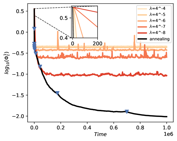
Results and discussions.

We repeat the simulations mentioned above for fixed $\lambda$’s and dynamic $\lambda_{\textnormal{a}}$ all for $100$ times and compute the averaged loss $\Phi(Y_{t})$ at each time $t$ and plot its evolution in Figure 1. On the annealing scheme curve, we include triangles to visually indicate the points at which there are changes on the values of $\lambda_{\textnormal{a}}$. We observe that the value of $\Phi(Y_{t})$ first decays exponentially, and the speed of initial decay depending on the value of $\lambda$. More precisely, the bigger is the value of $\lambda$, the faster is the initial decay. In particular, this remains true for the annealed process as it starts from a bigger value $\lambda_{\textnormal{a}}(0)$. We notice that such phenomenon is in line with our theoretical results in Theorem 1. In the long run, when fixing $\lambda$, the value of $\Phi(Y_{t})$ stabilizes at a level sensible with respect to the value of $\lambda$. We notice that the smaller is the value of $\lambda$, the better is the final performance. These facts are in line with our discovery in Theorems 1 and 3. Finally, the training exhibits the best performance when implementing the discrete annealing. The loss $\Phi(Y_{t})$ continues decreasing as the value of $\lambda_{\textnormal{a}}(t)$ diminishes, which confirms the result in Theorem 4.

4 Proof of Theorem 1

Proof of Theorem 1.

We first note that, as pointed out in Remark 1, the mapping $\iota:\mathcal{P}(\mathbb{R}^{d})\to E$ is continuous. Therefore, the separability of $\mathcal{P}(\mathbb{R}^{d})$ implies the separability of $\iota\bigl{(}\mathcal{P}(\mathbb{R}^{d})\bigr{)}$ as a subset of the Banach space $E$. This is sufficient to avoid the measurability issues for Banach-valued random variables and we refer readers to [30, Chapter 2] for details.

Denote $Y_{t}=\iota(m_{t})$, $Y^{\prime}_{t}=\iota(m^{\prime}_{t})$. Then the self-interacting dynamics (4) writes

$\displaystyle dX_{t}$ $\displaystyle=b(m_{t},X_{t})dt+dB_{t},$ (13)
$\displaystyle dY_{t}$ $\displaystyle=\lambda\bigl{(}-Y_{t}+\iota(\delta_{X_{t}})\bigr{)}dt$

and similarly for the other dynamics $(X^{\prime},Y^{\prime})$ driven by another Brownian motion $B^{\prime}$. Note that $X$ takes value in $\mathbb{R}^{d}$ and $Y$ takes value in the Banach space $E$. Fix $n\in\mathbb{N}$. Let $\textnormal{rc}:\mathbb{R}^{d}\times\mathbb{R}^{d}\to[0,1]$ be a Lipschitz continuous function such that $\textnormal{sc}\coloneqq\sqrt{1-\textnormal{rc}^{2}}$ is also Lipschitz continuous and

$$\textnormal{rc}(x,x^{\prime})=\begin{cases}1&\text{if}~{}|x-x^{\prime}|\geqslant 2n^{-1},\\ 0&\text{if}~{}|x-x^{\prime}|\leqslant n^{-1}.\end{cases}$$

We couple the two dynamics $(X,Y)$, $(X^{\prime},Y^{\prime})$ by

$\displaystyle dB_{t}$ $\displaystyle=\textnormal{rc}(X_{t},X^{\prime}_{t})dB^{\textnormal{rc}}_{t}+\textnormal{sc}(X_{t},X^{\prime}_{t})dB^{\textnormal{sc}}_{t},$
$\displaystyle dB^{\prime}_{t}$ $\displaystyle=\textnormal{rc}(X_{t},X^{\prime}_{t})\bigl{(}1-2e_{t}e_{t}^{\top}\bigr{)}dB^{\textnormal{rc}}_{t}+\textnormal{sc}(X_{t},X^{\prime}_{t})dB^{\textnormal{sc}}_{t},$

where $B^{\textnormal{rc}}$, $B^{\textnormal{sc}}$ are independent Brownian motions and $e_{t}$ is the $d$-dimensional vector defined by

$$e_{t}=\begin{cases}\frac{X_{t}-X^{\prime}_{t}}{|X_{t}-X^{\prime}_{t}|}&\text{if}~{}X_{t}\neq X^{\prime}_{t},\\ (1,0,\ldots,0)^{\top}&\text{otherwise}.\end{cases}$$

Subtracting the dynamical equations of $(X,Y)$, $(X^{\prime},Y^{\prime})$ and denoting $\delta X=X-X^{\prime}$, $\delta Y=Y-Y^{\prime}$, we obtain

$\displaystyle d\delta X_{t}$ $\displaystyle=\bigl{(}b(m_{t},X_{t})-b(m^{\prime}_{t},X^{\prime}_{t})\bigr{)}dt+2\textnormal{rc}(X_{t},X^{\prime}_{t})e_{t}dW_{t},$
$\displaystyle d\delta Y_{t}$ $\displaystyle=-\lambda\delta Y_{t}dt+\lambda\bigl{(}\iota(\delta_{X_{t}})-\iota(\delta_{X^{\prime}_{t}})\bigr{)}dt,$

where $W_{t}\coloneqq\int_{0}^{t}e_{t}^{\top}dB^{\textnormal{rc}}_{t}$ and is a one-dimensional Brownian motion by Lévy’s characterization. The absolute value of the semimartingale $\delta X_{t}$ admits the decomposition $d|\delta X_{t}|=dA^{|\delta X|}_{t}+dM^{|\delta X|}_{t}$ with

$\displaystyle dA^{|\delta X|}_{t}$ $\displaystyle\leqslant-|\delta X_{t}|\kappa(|\delta X_{t}|)dt+L\lVert\delta Y_{t}\rVert_{E}dt,$
$\displaystyle dM^{|\delta X|}_{t}$ $\displaystyle=2\textnormal{rc}(X_{t},X^{\prime}_{t})dW_{t}.$
The Banach-norm process $\lVert\delta Y\rVert_{E}$ is absolutely continuous and satisfies
$\displaystyle d\lVert\delta Y_{t}\rVert_{E}$ $\displaystyle\leqslant-\lambda\lVert\delta Y_{t}\rVert_{E}dt+\lambda\lVert\iota(\delta_{X_{t}})-\iota(\delta_{X^{\prime}_{t}})\rVert_{E}dt$
$\displaystyle\leqslant-\lambda\lVert\delta Y_{t}\rVert_{E}dt+\lambda\omega(\lvert\delta X_{t}\rvert)dt.$

Hence the process

$$r_{t}=\lambda\lvert\delta X_{t}\rvert+2L\lVert\delta Y_{t}\rVert_{E}$$

admits the decomposition $dr_{t}=dA^{r}_{t}+dM^{r}_{t}$ with

$\displaystyle dA^{r}_{t}$ $\displaystyle\leqslant\lambda\bigl{(}-\lvert\delta X_{t}\rvert\kappa(|\delta X_{t}|)+2L\omega(|\delta X_{t}|)-L\lVert\delta Y_{t}\rVert_{E}\bigr{)}dt,$
$\displaystyle dM^{r}_{t}$ $\displaystyle=2\textnormal{rc}(X_{t},X^{\prime}_{t})dW_{t}.$

Let $f:[0,\infty)\to[0,\infty)$ be a $\mathcal{C}^{2}$ function and define $\rho_{t}=f(r_{t})$. Then, the process $\rho_{t}$ admits the decomposition $d\rho_{t}=dA^{\rho}_{t}+dM^{\rho}_{t}$ with

$\displaystyle dA^{\rho}_{t}$ $\displaystyle\leqslant\lambda\bigl{(}-|\delta X_{t}|\kappa(|\delta X_{t}|)+2L\omega(|\delta X_{t}|)-L\lVert\delta Y_{t}\rVert_{E}\bigr{)}f^{\prime}_{-}(r_{t})dt$
$\displaystyle\hphantom{\leqslant{}}\quad+2\textnormal{rc}(X_{t},X^{\prime}_{t})^{2}f^{\prime\prime}(r_{t})dt$
$\displaystyle\leqslant-r_{t}\tilde{K}(r_{t})f^{\prime}_{-}(r_{t})dt+2\textnormal{rc}(X_{t},X^{\prime}_{t})^{2}f^{\prime\prime}(r_{t})dt$

for the function $\tilde{K}:(0,\infty)\to\mathbb{R}$ defined by

$\displaystyle\tilde{K}(r)$ $\displaystyle\coloneqq\inf_{\begin{subarray}{c}\lambda x+2Ly=r\\ x,y>0\end{subarray}}\frac{\lambda(x\kappa(x)-2L\omega(x)+Ly)}{r}$
$\displaystyle\geqslant\inf_{\begin{subarray}{c}\lambda x+2Ly=r\\ x,y>0\end{subarray}}\frac{\lambda(\kappa_{0}x+Ly-M_{b}-2LM_{\omega})}{r}$
$\displaystyle\geqslant\min\biggl{(}\kappa_{0},\frac{\lambda}{2}\biggr{)}-\frac{\lambda(M_{b}+2LM_{\omega})}{r}$
$\displaystyle\eqqcolon K_{0}-\frac{M}{r}\eqqcolon K(r).$

Thus, we have shown

$$dA^{\rho}_{t}\leqslant-r_{t}K(r_{t})f^{\prime}_{-}(r_{t})dt+2\textnormal{rc}(X_{t},X^{\prime}_{t})^{2}f^{\prime\prime}(r_{t})dt.$$

Following Du et al. [19], we choose the function $f:[0,\infty)\to[0,\infty)$ by requiring

$$f^{\prime}(r)=\frac{1}{2}\int_{r}^{\infty}s\exp\biggl{(}-\frac{1}{2}\int_{r}^{s}\tau K(\tau)d\tau\biggr{)}ds.$$

and $f(0)=0$. The function $f$ is indeed $\mathcal{C}^{2}$ continuous, and, according to [19, Lemma 5.1], it is also concave and satisfies

$$2f^{\prime\prime}(r)-rK(r)f^{\prime}(r)+r=0$$

and

$$\frac{1}{K_{0}}\leqslant f^{\prime}(r),\,\frac{f(r)}{r}\leqslant f^{\prime}(0)$$

for all $r>0$. Plugging in the expression for $K$, we obtain

$\displaystyle f^{\prime}(0)$ $\displaystyle=\frac{1}{2}\int_{0}^{\infty}s\exp\biggl{(}-\frac{K_{0}s^{2}}{4}+\frac{Ms}{2}\biggr{)}ds$
$\displaystyle=\frac{1}{2}\exp\biggl{(}\frac{M^{2}}{4K_{0}}\biggr{)}\int_{0}^{\infty}s\exp\biggl{(}-\frac{K_{0}(s-\frac{M}{K_{0}})^{2}}{4}\biggr{)}ds$
$\displaystyle=\frac{1}{2}\exp\biggl{(}\frac{M^{2}}{4K_{0}}\biggr{)}\int_{-M/\sqrt{2K_{0}}}^{\infty}\Biggl{(}\frac{2t}{K_{0}}+M\frac{2^{1/2}}{K_{0}^{3/2}}\Biggr{)}\exp\biggl{(}-\frac{t^{2}}{2}\biggr{)}dt$
$\displaystyle\leqslant\frac{1}{2}\exp\biggl{(}\frac{M^{2}}{4K_{0}}\biggr{)}\Biggl{(}\frac{2}{K_{0}}\exp\biggl{(}-\frac{M^{2}}{4K_{0}}\biggr{)}+2M\frac{\pi^{1/2}}{K_{0}^{3/2}}\Biggr{)}$
$\displaystyle\leqslant\frac{1}{K_{0}}+\frac{2M}{K_{0}^{3/2}}\exp\biggl{(}\frac{M^{2}}{4K_{0}}\biggr{)}.$

Thus, if $|\delta X_{t}|\geqslant 2n^{-1}$, then $\textnormal{rc}_{t}(X_{t},X^{\prime}_{t})=1$, and

$$df(r_{t})=dA^{\rho}_{t}+dM^{\rho}_{t}\leqslant-r_{t}dt+dM^{\rho}_{t}\leqslant-\frac{f(r_{t})}{K_{0}^{-1}+2MK_{0}^{-3/2}\exp(M^{2}/4K_{0})}dt+dM^{\rho}_{t}.$$

Otherwise, $|\delta X_{t}|<2n^{-1}$, and denoting by $\omega_{b}$ the uniform modulus of equicontinuity of the vector fields $x\mapsto b(m,x)$, we have

$\displaystyle dA^{\rho}_{t}$ $\displaystyle\leqslant\lambda\bigl{(}\omega_{b}(2n^{-1})+2L\omega(2n^{-1})-L\lVert\delta Y_{t}\rVert_{E}\bigr{)}f^{\prime}(r_{t})dt$
$\displaystyle=-\lambda Lf^{\prime}(r_{t})\lVert\delta Y_{t}\rVert_{E}dt+o(1)dt$
$\displaystyle\leqslant-\frac{\lambda L}{K_{0}}\lVert\delta Y_{t}\rVert_{E}dt+o(1)dt$
$\displaystyle=-\frac{\lambda}{2K_{0}}r_{t}dt+o(1)dt$
$\displaystyle\leqslant-r_{t}dt+o(1)dt$
$\displaystyle\leqslant-\frac{f(r_{t})}{K_{0}^{-1}+2MK_{0}^{-3/2}\exp(M^{2}/4K_{0})}dt+o(1)dt,$

where the $o(1)$ terms may change from line to line, but all tend to 00 when $n\to\infty$. Then, combining the two cases above, we obtain, by Grönwall’s lemma,

$$\operatorname{\mathbb{E}}[f(r_{t})]\leqslant e^{-ct}\operatorname{\mathbb{E}}[f(r_{0})]+o(1),$$

for $c=\bigl{(}K_{0}^{-1}+2MK_{0}^{-3/2}\exp(M^{2}/4K_{0})\bigr{)}^{-1}$, and we conclude by taking the limit $n\to\infty$. ∎

5 Proof of Theorem 3

In this section we establish several intermediate results before giving the proof of Theorem 3.

We first note that the stationary measure, which exists according to Assumption 4, solves a partial differential equation in the following weak sense.

Proposition 5.

Let $\mathcal{C}^{1,2}_{\textnormal{b}}$ denote the class of functionals $\phi:\mathcal{P}(\mathbb{R}^{d})\times\mathbb{R}^{d}\to\mathbb{R}$ with continuous spatial derivatives $\nabla_{x}\phi$, $\nabla_{x}^{2}\phi$ and a bounded linear functional derivative $\frac{\delta\phi}{\delta m}:\mathcal{P}(\mathbb{R}^{d})\times\mathbb{R}^{d}\times\mathbb{R}^{d}\to\mathbb{R}$ satisfying

$\displaystyle\forall m\in\mathcal{P}(\mathbb{R}^{d}),~{}\forall x\in\mathbb{R}^{d},$ $\displaystyle\lvert\nabla_{x}\phi(m,x)\rvert+\bigl{|}\nabla_{x}^{2}\phi(m,x)\bigr{|}$ $\displaystyle\leqslant C,$
$\displaystyle\forall m\in\mathcal{P}(\mathbb{R}^{d}),~{}\forall x,x^{\prime}\in\mathbb{R}^{d},$ $\displaystyle\biggl{|}\frac{\delta\phi}{\delta m}(m,x,x^{\prime})\biggr{|}$ $\displaystyle\leqslant C,$

for some $C\geqslant 0$. Under Assumptions 3, and 4, let $(X,m)$ be a random variable distributed as the stationary measure $P$. Then we have, for all $\phi\in\mathcal{C}^{1,2}_{\textnormal{b}}$,

$$\operatorname{\mathbb{E}}\biggl{[}\frac{1}{2}\Delta_{x}\phi(m,X)+b(m,X)\cdot\nabla_{x}\phi(m,X)\\ +\lambda\int\frac{\delta\phi}{\delta m}(m,X,x^{\prime})(\delta_{X}-m)(dx^{\prime})\biggr{]}=0.$$

We omit the proof of the proposition, which follows directly from developing the difference $\operatorname{\mathbb{E}}[\phi(m_{t},X_{t})]-\operatorname{\mathbb{E}}[\phi(m_{0},X_{0})]$ by Itō-type calculus.

The infinite-dimensional nature of the PDE above makes its analysis difficult, and in the following we approach the problem by studying a finite-dimensional projection of it. Under Assumption 3, define the functions

$\displaystyle\beta(y,x)$ $\displaystyle=-\nabla\Phi(y)\cdot\nabla\ell(x)=-\sum_{\nu=1}^{D}\nabla_{\nu}\Phi(y)\nabla\ell^{\nu}(x),$
$\displaystyle V(y,x)$ $\displaystyle=\nabla\Phi(y)\cdot\ell(x)=\sum_{\nu=1}^{D}\nabla_{\nu}\Phi(y)\ell^{\nu}(x).$

They verify $\beta(y,x)=-\nabla_{x}V(y,x)$. Note that, if $m_{y}$ is a measure satisfying $\int\ell(x)m_{y}(dx)=y$, then we have

$\displaystyle\beta(y,x)$ $\displaystyle=b(m_{y},x),$
$\displaystyle V(y,x)$ $\displaystyle=\frac{\delta F}{\delta m}(m_{y},x).$

Let $(X,m)$ be distributed as the stationary measure $P$ in Assumption 4. Setting $Y=\langle\ell,m\rangle=\int\ell(x)m(dx)$ and applying Proposition 5 to functionals of the following form:

$$\phi(m,x)=\varphi\biggl{(}x,\int\ell(x^{\prime})m(dx^{\prime})\biggr{)},$$

where $\varphi\in\mathcal{D}(\mathbb{R}^{d}\times\mathbb{R}^{D})$, we get that the joint distribution $\rho=\rho^{\lambda}\coloneqq\operatorname{Law}(X,Y)\in\mathcal{P}(\mathbb{R}^{d}\times\mathbb{R}^{D})$ satisfies the static degenerate Fokker–Planck equation

$$\frac{1}{2}\Delta_{x}\rho-\nabla_{x}\cdot\bigl{(}\beta(y,x)\rho\bigr{)}-\lambda\nabla_{y}\cdot\Bigl{(}\bigl{(}\ell(x)-y\bigr{)}\rho\Bigr{)}=0.$$ (14)

in the sense of distributions. The fact that $P$ has finite fourth moment implies that its projection $\rho$ satisfies the following moment condition:

$$\int(\lvert x\rvert^{4}+\lvert y\rvert^{2})\rho(dxdy)<\infty.$$ (15)

In the following, we will denote the first and second marginal distributions of $\rho$ by $\rho^{1}$, $\rho^{2}$ respectively, and the conditional distributions to the second variable by $\rho^{1|2}:\mathcal{B}(\mathbb{R}^{d})\times\mathbb{R}^{D}\to\mathbb{R}$. Define

$$\hat{\rho}(dxdy)\coloneqq\hat{m}_{y}(dx)\rho^{2}_{t}(dy)=\frac{1}{Z_{y}}\exp\bigl{(}-2V(y,x)\bigr{)}dx\rho^{2}_{t}(dy),$$ (16)

for $Z_{y}=\int\exp\bigl{(}-2V(y,x)\bigr{)}dx$. Recall that $\hat{m}_{y}$ is the probability measure on $\mathbb{R}^{d}$ that satisfies a uniform LSI according to Assumption 5.

From the Fokker–Planck equation (14), we get the following result.

Lemma 6.

Under Assumption 3 and 4, for every function $\varphi\in\mathcal{C}^{1}(\mathbb{R}^{D};\mathbb{R})$ whose gradient $\nabla\varphi$ is of linear growth, we have

$$\iint\nabla\varphi(y)\cdot\bigl{(}\ell(x)-y\bigr{)}\rho(dxdy)=0.$$
Proof of Lemma 6.

Since its gradient $\nabla\varphi$ is of linear growth, the function $\varphi$ is of quadratic growth. Thanks to the fact that $\rho$ satisfies the moment condition (15), we can take the duality with $\varphi$ in the static Fokker–Planck equation (14), from which the desired result follows. ∎

Then, by studying the more carefully the Fokker–Planck equation (14), we can control the relative entropy between $\rho$ and $\hat{\rho}$, the latter being introduced in (16).

Proposition 7.

Suppose Assumptions 3, 4 and 5 hold true. Then,

$$H(\rho|\hat{\rho})\leqslant\frac{C_{\textnormal{LS}}}{2}\biggl{(}D+2\iint\bigl{(}\ell(x)-y\bigr{)}^{\top}\nabla^{2}\Phi(y)\bigl{(}\ell(x)-y\bigr{)}\rho(dxdy)\biggr{)}\lambda,$$

where $\hat{\rho}$ is the measure defined by (16).

In the following, we denote

$$I\coloneqq\iint\bigl{(}\ell(x)-y\bigr{)}^{\top}\nabla^{2}\Phi(y)\bigl{(}\ell(x)-y\bigr{)}\rho(dxdy),$$ (17)

so the result of the proposition reads

$$H(\rho|\hat{\rho})\leqslant\frac{C_{\textnormal{LS}}}{2}(D+2I)\lambda.$$
Proof of Proposition 7.

Let $g^{\varepsilon}$ be the Gaussian kernel in $D$ dimensions:

$$g^{\varepsilon}(y)=(2\pi\varepsilon)^{-D/2}\exp\biggl{(}-\frac{|y|^{2}}{2\varepsilon}\biggr{)}.$$

We define the partial convolution $\rho^{\varepsilon}=\rho\star_{y}g^{\varepsilon}$, and according to (14), it solves the non-degenerate elliptic equation

$$\frac{1}{2}\Delta_{x}\rho^{\varepsilon}-\nabla_{x}\cdot\bigl{(}\beta^{\varepsilon}(y,x)\rho^{\varepsilon}\bigr{)}-\ell(x)\cdot\nabla_{y}\rho^{\varepsilon}+\lambda\varepsilon\Delta_{y}\rho^{\varepsilon}+\lambda\nabla_{y}\cdot(y\rho^{\varepsilon})=0,$$ (18)

where $\beta^{\varepsilon}$ is defined by

$$\beta^{\varepsilon}=\frac{(\beta\rho)\star_{y}g^{\varepsilon}}{\rho^{\varepsilon}}.$$

Indeed, we have

$\displaystyle(y\rho)\star_{y}g^{\varepsilon}$ $\displaystyle=\int y^{\prime}\rho(x^{\prime},y^{\prime})g^{\varepsilon}(y-y^{\prime})dy^{\prime}$
$\displaystyle=\int(y^{\prime}-y+y)\rho(x^{\prime},y^{\prime})g^{\varepsilon}(y-y^{\prime})dy^{\prime}$
$\displaystyle=\varepsilon\int\rho(x^{\prime},y^{\prime})\nabla_{y}g^{\varepsilon}(y-y^{\prime})dy^{\prime}+y\rho^{\varepsilon}$
$\displaystyle=\varepsilon\nabla_{y}\rho^{\varepsilon}+y\rho^{\varepsilon}.$

Thus, $\bigl{(}\nabla_{y}\cdot(y\rho)\bigr{)}\star_{y}g^{\varepsilon}=\nabla_{y}\cdot\bigl{(}(y\rho)\star_{y}g^{\varepsilon}\bigr{)}=\varepsilon\Delta_{y}\rho^{\varepsilon}+\nabla_{y}\cdot(y\rho^{\varepsilon})$. By [5, Lemma 3.1.1], we have $\lVert\beta^{\varepsilon}\rVert_{L^{2}(\rho^{\varepsilon})}\leqslant\lVert\beta\rVert_{L^{2}(\rho)}<\infty$. Then we can apply [5, Theorem 3.1.2] to (18) and obtain that $\rho^{\varepsilon}\in W^{1,1}(\mathbb{R}^{d+D})$ and satisfies

$$\frac{1}{2}\iint\frac{|\nabla_{x}\rho^{\varepsilon}|^{2}}{\rho^{\varepsilon}}+\lambda\varepsilon\iint\frac{|\nabla_{y}\rho^{\varepsilon}|^{2}}{\rho^{\varepsilon}}\\ =\iint\nabla_{x}\rho^{\varepsilon}\cdot\beta^{\varepsilon}+\lambda\iint\nabla_{y}\rho^{\varepsilon}\cdot\ell-\lambda\iint\nabla_{y}\rho^{\varepsilon}\cdot y.$$

As the function $\ell$ depends only on the $x$ argument, for the second term we have

$$\iint\nabla_{y}\rho^{\varepsilon}\cdot\ell=\int\biggl{(}\int\nabla_{y}\rho^{\varepsilon}(x,y)dy\biggr{)}\ell(x)dx=\int 0\cdot\ell(x)dx=0.$$

where the first equality is due to Fubini and the second to the fact that $\nabla\rho^{\varepsilon}\in L^{1}_{x}(L^{1}_{y})$. For the last term, similarly, since the function $\bigl{(}(x,y)\mapsto\rho^{\varepsilon}(x,y)y\bigr{)}\in W^{1,1}$, we have $\iint\nabla_{y}\cdot(\rho^{\varepsilon}y)=0$ and therefore,

$$-\iint\nabla_{y}\rho^{\varepsilon}\cdot y=\iint(\nabla_{y}\cdot y)\rho^{\varepsilon}=D.$$

That is to say, we have established

$$\frac{1}{2}\iint\frac{|\nabla_{x}\rho^{\varepsilon}|^{2}}{\rho^{\varepsilon}}+\lambda\varepsilon\iint\frac{|\nabla_{y}\rho^{\varepsilon}|^{2}}{\rho^{\varepsilon}}=\iint\nabla_{x}\rho^{\varepsilon}\cdot\beta^{\varepsilon}+\lambda D.$$ (19)

This equality implies a uniform-in-$\varepsilon$ bound on $\iint|\nabla_{x}\rho^{\varepsilon}|^{2}/\rho^{\varepsilon}$ by Cauchy–Schwarz. Using a sequence of functions in $\mathcal{C}^{\infty}_{\textnormal{c}}$ approaching $V(y,x)$ in (14), we also get

$$\iint\frac{1}{2}\beta\cdot\nabla_{x}\rho^{\varepsilon}-\iint\lambda\varepsilon\nabla_{y}V\cdot\nabla_{y}\rho^{\varepsilon}-\iint\beta\cdot\beta^{\varepsilon}\rho^{\varepsilon}\\ +\iint\lambda\nabla_{y}V(y,x)\cdot\bigl{(}\ell(x)-y\bigr{)}\rho^{\varepsilon}(dxdy)=0.$$ (20)

The second term of (20) is upper bounded by

$\displaystyle\lambda\varepsilon\iint\lvert\nabla_{y}V\cdot\nabla_{y}\rho^{\varepsilon}\rvert$ $\displaystyle\leqslant\lambda\varepsilon\lVert\nabla_{y}V\rVert_{L^{2}(\rho^{\varepsilon})}\biggl{(}\iint\frac{|\nabla_{y}\rho^{\varepsilon}|^{2}}{\rho^{\varepsilon}}\biggr{)}^{\!1/2}$
$\displaystyle\leqslant\sqrt{\lambda\varepsilon}\lVert\nabla_{y}V\rVert_{L^{2}(\rho^{\varepsilon})}\sqrt{\frac{1}{2}\iint\frac{|\nabla_{x}\rho^{\varepsilon}|^{2}}{\rho^{\varepsilon}}+\frac{1}{2}\lVert\beta^{\varepsilon}\rVert_{L^{2}(\rho^{\varepsilon})}^{2}+\lambda D},$

where the second inequality is due to (19). Using the uniform-in-$\varepsilon$ bound of $\iint\lvert\nabla_{x}\rho^{\varepsilon}\rvert^{2}/\rho^{\varepsilon}$, we obtain that the second term of (20) converges to 00 when $\varepsilon\to 0$. The third term of (20) satisfies

$$\iint\beta\cdot\beta^{\varepsilon}\rho^{\varepsilon}=\iint\beta\cdot\bigl{(}(\beta\rho)\star g^{\varepsilon}\bigr{)}=\iint(\beta\star g^{\varepsilon})\cdot\beta\rho\to\iint|\beta|^{2}\rho$$

when $\varepsilon\to 0$. Hence, by (19) and (20), we have

$\displaystyle\frac{1}{2}\iint|\nabla_{x}\log\rho^{\varepsilon}-2\beta|^{2}\rho^{\varepsilon}(dxdy)$
$\displaystyle\leqslant\lambda D+\iint\nabla_{x}\rho^{\varepsilon}\cdot\beta^{\varepsilon}+\iint\beta\cdot\nabla_{x}\rho^{\varepsilon}-2\iint\nabla_{x}\rho^{\varepsilon}\cdot\beta$
$\displaystyle\hphantom{\leqslant{}}\quad+2\lambda\iint\nabla_{y}V(y,x)\cdot\bigl{(}\ell(x)-y\bigr{)}\rho^{\varepsilon}(dxdy)+o(1)$
$\displaystyle=\lambda D+2\lambda\iint\nabla_{y}V(y,x)\cdot\bigl{(}\ell(x)-y\bigr{)}\rho^{\varepsilon}(dxdy)+o(1),$

where the last equality is due to the fact that

$$\biggl{|}\iint\nabla_{x}\rho^{\varepsilon}\cdot(\beta^{\varepsilon}-\beta)\biggr{|}\leqslant\biggl{(}\iint\frac{|\nabla_{x}\rho^{\varepsilon}|^{2}}{\rho^{\varepsilon}}\biggr{)}^{\!1/2}\biggl{(}\iint|\beta-\beta^{\varepsilon}|^{2}\rho^{\varepsilon}\biggr{)}^{\!1/2}$$

and

$\displaystyle\iint|\beta-\beta^{\varepsilon}|^{2}\rho^{\varepsilon}$ $\displaystyle=\iint|\beta|^{2}\rho^{\varepsilon}-2\iint\beta\cdot\beta^{\varepsilon}\rho^{\varepsilon}+\iint|\beta^{\varepsilon}|^{2}\rho^{\varepsilon}$
$\displaystyle=\iint(|\beta|^{2}\star_{y}g^{\varepsilon})\rho-2\iint(\beta\star_{y}g^{\varepsilon})\cdot\beta\rho+\iint|\beta^{\varepsilon}|^{2}\rho^{\varepsilon}\to 0,$

when $\varepsilon\to 0$ by previous arguments and [5, Lemma 3.1.1]. We also have

$$\iint\nabla_{y}V(y,x)\cdot\bigl{(}\ell(x)-y\bigr{)}\rho^{\varepsilon}(dxdy)=\iint\Bigl{(}\nabla_{y}V(y,x)\cdot\bigl{(}\ell(x)-y\bigr{)}\Bigr{)}\star_{y}g^{\varepsilon}\rho(dxdy)\\ \to\iint\nabla_{y}V(y,x)\cdot\bigl{(}\ell(x)-y\bigr{)}\rho(dxdy)$$

when $\varepsilon\to 0$. Finally, by Lemma 6 for the function $\varphi(y)=y\cdot\nabla\Phi(y)-\Phi(y)$, we have

$\displaystyle\iint\nabla_{y}V(y,x)\cdot\bigl{(}\ell(x)-y\bigr{)}\rho(dxdy)$
$\displaystyle=\iint\ell(x)^{\top}\nabla^{2}\Phi(y)\bigl{(}\ell(x)-y\bigr{)}\rho(dxdy)$
$\displaystyle=\iint\bigl{(}\ell(x)-y\bigr{)}^{\top}\nabla^{2}\Phi(y)\bigl{(}\ell(x)-y\bigr{)}\rho(dxdy)=I,$

where the last equality is exactly the definition (17) of $I$. Thus, we have shown

$$\frac{1}{2}\iint\biggl{|}\nabla_{x}\log\frac{\rho^{\varepsilon}(x,y)}{\hat{m}_{y}(x)}\biggr{|}^{2}\rho^{\varepsilon}(dxdy)\leqslant(D+2I)\lambda.$$ (21)

The uniform LSI for $\hat{m}_{y}$ implies

$$H(\rho^{\varepsilon}|\hat{\rho}^{\varepsilon})=\int H\bigl{(}\rho^{1|2}(\cdot|y)\big{|}\hat{m}_{y}\bigr{)}\rho^{2}(dy)\leqslant\frac{C_{\textnormal{LS}}}{4}\!\iint\biggl{|}\nabla_{x}\log\frac{\rho^{\varepsilon}(x,y)}{\hat{m}_{y}(x)}\biggr{|}^{2}\rho^{\varepsilon}(dxdy).$$

Hence,

$$H(\rho^{\varepsilon}|\hat{\rho}^{\varepsilon})\leqslant\frac{C_{\textnormal{LS}}}{2}(D+2I)\lambda+o(1).$$

Taking into account of the lower semi-continuity of relative entropy under the weak convergence, and the weak convergences $\rho^{\varepsilon}\to\rho$, $\hat{\rho}^{\varepsilon}\to\hat{\rho}$, we take the limit $\varepsilon\to 0$ in the inequality above to conclude. ∎

Remark 5.

If we formally integrate the static Fokker–Planck equation (14) with $\log(\rho/\hat{\rho})$ and integrate by parts, we obtain

$$\frac{1}{2}\iint\biggl{|}\nabla_{x}\log\frac{\rho(x,y)}{\hat{m}_{y}(x)}\biggr{|}^{2}\rho(dxdy)=\lambda D+2\lambda\iint\ell(x)^{\top}\nabla^{2}\Phi(y)\bigl{(}\ell(x)-y\bigr{)}\rho(dxdy).$$ (22)

However, the equality must be false. Indeed, if one artificially increases the dimension of $\ell$ and $\Phi$ by defining the new functions

$\displaystyle\tilde{\Phi}(y_{0},y_{1})$ $\displaystyle=\Phi(y_{0}),$
$\displaystyle\tilde{\ell}(x)$ $\displaystyle=\bigl{(}\ell(x),0\bigr{)},$

the right hand side of (22) increases while the left hand side stays unchanged. This phenomenon is caused by the fact that the equation (14) is degenerate elliptic and lacks Laplacian in the $y$ directions. To illustrate this effect, consider the first-order equation

$$\nabla_{y}\cdot(y\rho)=0$$

in $d$ dimensions. This equation has a probability solution $\rho=\delta_{0}$, the Dirac mass at the origin. Formally integrating the equation with $\log\rho$ and integrating by parts, we have

$$0=\int\log\rho\nabla_{y}\cdot(y\rho)=-\int\frac{\nabla_{y}\rho}{\rho}\cdot y\rho=-\int\nabla_{y}\rho\cdot y=\int\rho\nabla_{y}\cdot y=\int\rho d=d,$$

which is absurd.

We establish in the following upper bounds for the integral $I$.

Proposition 8.

Under Assumptions 3, 4 and 5, the integral $I$ in (17) satisfies the upper bound:

$$I\leqslant 12M_{2}\Bigl{(}dC_{\textnormal{LS}}+2W_{2}^{2}\bigl{(}\operatorname{Law}(X),m_{*}\bigr{)}\Bigr{)},$$ (23)

where $X$ is the first component of the random variable $(X,m)$ following the stationary distribution $P=P^{\lambda}$, and $m_{*}$ is the unique invariant measure of the McKean–Vlasov process (1). If additionally the quantity

$$M_{1}\coloneqq\sup_{x\in\mathbb{R}^{d},y\in\mathbb{R}^{D}}\ell(x)^{\top}\nabla^{2}\Phi(y)\ell(x)$$

is finite, then we have the alternative upper bound:

$$I\leqslant M_{1}.$$ (24)
Proof of Proposition 8.

First let us treat the simpler case where $M_{1}<\infty$. By applying Lemma 6 to the function $\varphi(y)=y\cdot\nabla\Phi(y)-\Phi(y)$, we get

$\displaystyle I$ $\displaystyle=\iint\bigl{(}\ell(x)^{\top}\nabla^{2}\Phi(y)\ell(x)-y^{\top}\nabla^{2}\Phi(y)y\bigr{)}\rho(dxdy)$
$\displaystyle\leqslant\iint\ell(x)^{\top}\nabla^{2}\Phi(y)\ell(x)\rho(dxdy)\leqslant M_{1}.$

So the second claim of the proposition is proved.

Without the assumption $M_{1}<\infty$, we note that, for the second-order functional derivative

$$\frac{\delta^{2}F}{\delta m^{2}}(m,x^{\prime},x^{\prime\prime})=\ell(x^{\prime\prime})^{\top}\nabla^{2}\Phi(\langle\ell,m\rangle)\ell(x),$$

we have

$$I=\operatorname{\mathbb{E}}\biggl{[}\iint\frac{\delta^{2}F}{\delta m^{2}}(m,x^{\prime},x^{\prime\prime})(\delta_{X}-m)(dx^{\prime})(\delta_{X}-m)(dx^{\prime\prime})\biggr{]},$$

where $(X,m)$ is a random variable following the stationary distribution $P$, and $(X,\langle\ell,m\rangle)$ has the distribution $\rho$. We observe

$\displaystyle\bigl{|}D_{m}^{2}F(m,x^{\prime},x^{\prime\prime})\bigr{|}$ $\displaystyle=\biggl{|}\nabla_{x^{\prime}}\nabla_{x^{\prime\prime}}\frac{\delta^{2}F}{\delta m^{2}}(m,x^{\prime},x^{\prime\prime})\biggr{|}$
$\displaystyle=\bigl{|}\nabla\ell(x^{\prime\prime})^{\top}\nabla^{2}\Phi(\langle\ell,m\rangle)\nabla\ell(x^{\prime})\bigr{|}\leqslant M_{2}.$

Then, by applying Lemma 12 in Appendix B to a sequence of $\mathcal{C}^{2}$ functions approaching $(x^{\prime},x^{\prime\prime})\mapsto\frac{\delta^{2}F}{\delta m^{2}}(m,x^{\prime},x^{\prime\prime})$, we get

$\displaystyle I$ $\displaystyle\leqslant M_{2}\operatorname{\mathbb{E}}\bigl{[}W_{2}^{2}(\delta_{X},m)\bigr{]}$
$\displaystyle=M_{2}\operatorname{\mathbb{E}}\biggl{[}\int\lvert X-x^{\prime}\rvert^{2}m(dx^{\prime})\biggr{]}$
$\displaystyle\leqslant 2M_{2}\operatorname{\mathbb{E}}\biggl{[}\lvert X-\operatorname{\mathbb{E}}[X]\rvert^{2}+\int\lvert x^{\prime}-\operatorname{\mathbb{E}}[X]\rvert^{2}m(dx^{\prime})\biggr{]}.$

Let $\phi:\mathcal{P}_{2}(\mathbb{R}^{d})\to\mathbb{R}$ be the functional defined by

$$\phi(m)=\int\lvert x^{\prime}-\operatorname{\mathbb{E}}[X]\rvert^{2}m(dx^{\prime}).$$

We consider the sequence of “soft cut-offs” of class $C^{1}_{\textnormal{b}}$ approaching $\phi$:

$$\phi_{n}(m)=\sum_{i=1}^{d}\int n^{2}\tanh^{2}\biggl{(}\frac{x^{\prime i}-\operatorname{\mathbb{E}}[X^{i}]}{n}\biggr{)}m(dx^{\prime}),\qquad\text{for}~{}n\in\mathbb{N}.$$

Then, by applying the sequence $\phi_{n}$ to Proposition 5 of stationary measure and taking the limit $n\to\infty$, we get

$$0=\lambda\operatorname{\mathbb{E}}\biggl{[}\int\frac{\delta\phi}{\delta m}(m,x^{\prime})(\delta_{X}-m)(dx^{\prime})\biggr{]}\\ =\lambda\operatorname{\mathbb{E}}\bigl{[}\lvert X-\operatorname{\mathbb{E}}[X]\lvert^{2}\bigr{]}-\lambda\operatorname{\mathbb{E}}\biggr{[}\!\int\lvert x^{\prime}-\operatorname{\mathbb{E}}[X]\rvert^{2}m(dx^{\prime})\biggr{]}.$$

Thus, we have derived

$$I\leqslant 4M_{2}\operatorname{\mathbb{E}}\bigl{[}\lvert X-\operatorname{\mathbb{E}}[X]\rvert^{2}\bigr{]}=4M_{2}\operatorname{Var}X,$$

and it remains to find an upper bound for $\operatorname{Var}X$. Note that, using the definition of Wasserstein distance and the triangle inequality, and letting $X_{*}$ be distributed as $m_{*}$, we get

$\displaystyle\operatorname{Var}X$ $\displaystyle=W_{2}^{2}\bigl{(}\operatorname{Law}(X),\delta_{\operatorname{\mathbb{E}}[X]}\bigr{)}$
$\displaystyle\leqslant 3\Bigl{(}W_{2}^{2}\bigl{(}\operatorname{Law}(X),m_{*}\bigr{)}+W_{2}^{2}\bigl{(}m_{*},\delta_{\operatorname{\mathbb{E}}[X_{*}]}\bigr{)}+W_{2}^{2}\bigl{(}\delta_{\operatorname{\mathbb{E}}[X_{*}]},\delta_{\operatorname{\mathbb{E}}[X]}\bigr{)}\Bigr{)}$
$\displaystyle\leqslant 3\Bigl{(}\operatorname{Var}X_{*}+2W_{2}^{2}\bigl{(}\operatorname{Law}(X),m_{*}\bigr{)}\Bigr{)},$

while the variance of $X_{*}$ is upper bounded by the Poincaré inequality:

$\displaystyle\operatorname{Var}X_{*}$ $\displaystyle=\sum_{i=1}^{d}\Biggl{(}\int\lvert x^{i}\rvert^{2}m_{*}(dx)-\biggl{(}\int x^{i}m_{*}(dx)\biggr{)}^{\!2}\Biggr{)}$
$\displaystyle\leqslant C_{\textnormal{LS}}\sum_{i=1}^{d}\int\lvert\nabla x^{i}\rvert^{2}m_{*}(dx)=C_{\textnormal{LS}}d.$

We then conclude by combining the three inequalities above. ∎

Before moving on to the proof of Theorem 3, we need to introduce another probability measure $\mu=\mu^{\lambda}$ on $\mathbb{R}^{d}\times\mathbb{R}^{D}$ characterized by the following formula:

$$\langle f,\mu\rangle=\int f(x,y)\mu(dxdy)\\ =\operatorname{\mathbb{E}}\biggl{[}\int f(x,\langle\ell,m\rangle)m(dx)\biggr{]}=\operatorname{\mathbb{E}}\biggl{[}\int f(x,Y)m(dx)\biggr{]}$$ (25)

for all bounded and measurable $f:\mathbb{R}^{d}\times\mathbb{R}^{D}\to\mathbb{R}$. By taking $f$ depending only on the $y$ variable, we first realize that the second marginals of $\rho$ and $\mu$ agree, that is,

$$\rho^{2}=\mu^{2}.$$

In addition, we show the following important properties of $\mu$.

Proposition 9.

Under Assumptions 3 and 4, for every $\mathcal{C}^{2}$ differentiable $\Psi:\mathbb{R}^{D}\to\mathbb{R}$ with bounded Hessian, we have

$$\iint\nabla\Psi(y)\cdot\ell(x)(\mu-\rho)(dxdy)=0.$$

In particular, the respective first marginals $\mu^{1}$, $\rho^{1}$ of $\mu$, $\rho$ satisfy

$$\int\ell(x)(\mu^{1}-\rho^{1})(dx)=0.$$

Moreover, denoting by $\mu^{1|2}(\cdot|\cdot):\mathcal{B}(\mathbb{R}^{d})\times\mathbb{R}^{D}\to\mathbb{R}$ the conditional measure of $\mu$ given its second variable. we have for $\rho^{2}$-a.s. $y\in\mathbb{R}^{D}$,

$$\bigl{\langle}\ell,\mu^{1|2}(\cdot|y)\bigr{\rangle}=y.$$
Proof of Proposition 9.

Consider the functional

$$\phi(m)=\int f(x^{\prime},\langle k,m\rangle)m(dx^{\prime}),$$

where $f\in\mathcal{C}^{1}_{\textnormal{b}}(\mathbb{R}^{d}\times\mathbb{R}^{D};\mathbb{R})$ and $k\in\mathcal{C}_{\textnormal{b}}(\mathbb{R}^{d};\mathbb{R}^{D})$. Then its linear functional derivative reads

$$\frac{\delta\phi}{\delta m}(m,x^{\prime})=f(x^{\prime},\langle k,m\rangle)+\int\nabla_{y}f(x^{\prime\prime},\langle k,m\rangle)\cdot k(x^{\prime})m(dx^{\prime\prime}),$$

so $\phi$ belongs to the $\mathcal{C}^{1}_{\textnormal{b}}$ class. Then, applying Proposition 5 to the functional $\phi$, we get

$\displaystyle 0$ $\displaystyle=\operatorname{\mathbb{E}}\biggl{[}\int\frac{\delta\phi}{\delta m}(m,x^{\prime})(\delta_{X}-m)(dx^{\prime})\biggr{]}$
$\displaystyle=\operatorname{\mathbb{E}}[f(X,m)]-\operatorname{\mathbb{E}}\biggl{[}\int f(x^{\prime},\langle k,m\rangle)m(dx^{\prime})\biggr{]}$
$\displaystyle\hphantom{={}}\quad+\operatorname{\mathbb{E}}\biggl{[}\int\nabla_{y}f(x^{\prime},\langle k,m\rangle)\cdot\bigl{(}k(X)-\langle k,m\rangle\bigr{)}m(dx^{\prime})\biggr{]}$

By approximation, the equality above holds for $k=\ell$ and for all $\mathcal{C}^{1}$-continuous $f$ with the following growth bounds:

$\displaystyle\lvert f(x,y)\rvert$ $\displaystyle\leqslant M(1+\lvert x\rvert^{4}+\lvert y\rvert^{2}),$
$\displaystyle\lvert\nabla_{y}f(x,y)\rvert$ $\displaystyle\leqslant M(1+\lvert x\rvert^{2}+\lvert y\rvert),$

that is to say, we have

$$\langle f,\rho-\mu\rangle+\operatorname{\mathbb{E}}\biggl{[}\int\nabla_{y}f(x^{\prime},Y)\bigl{(}\ell(X)-Y\bigr{)}m(dx^{\prime})\biggr{]}=0,$$

where, as before, $Y=\langle\ell,m\rangle$. Specializing to $f(x,y)=\nabla\Psi(y)\cdot\ell(x)$, we obtain

$\displaystyle\langle f,\mu-\rho\rangle$ $\displaystyle=\operatorname{\mathbb{E}}\biggl{[}\int\ell(x)^{\top}\nabla^{2}\Psi(Y)\bigl{(}\ell(X)-Y\bigr{)}m(dx)\biggr{]}$
$\displaystyle=\operatorname{\mathbb{E}}\bigl{[}Y^{\top}\nabla^{2}\Psi(Y)\bigl{(}\ell(X)-Y\bigr{)}\bigr{]}=0,$

where the last equality is due to Lemma 6, as for $\varphi(y)\coloneqq\nabla\Psi(y)\cdot y-\Psi(y)$, we have $\nabla\varphi(y)=\nabla^{2}\Psi(y)y$. So the first claim is proved. Taking $\Psi(y)=y^{\nu}$, for $\nu=1,\ldots,D$, yields the second claim.

For the last claim, we take $f(x,y)=\ell(x)g(y)$ for $g:\mathbb{R}^{D}\to\mathbb{R}$ of linear growth in the defining equation (25) of $\mu$. Then, we get

$$\int g(y)\biggl{(}\int\ell(x)\mu^{1|2}(dx|y)\biggr{)}\mu^{2}(dy)=\iint f(x,y)\mu(dxdy)=\operatorname{\mathbb{E}}[Yg(Y)]\\ =\int g(y)y\mu^{2}(dy).$$

The desired property follows from the arbitrariness of $g$. ∎

Proof of Theorem 3.

The proof consists of five steps.

Step 1: Control of the symmetrized entropy. We aim at controlling the symmetrized entropy

$$\int\bigl{(}H(\hat{m}_{y}|m_{*})+H(m_{*}|\hat{m}_{y})\bigr{)}\rho^{2}(dy)$$

in this step. First observe

$$\int\bigl{(}H(\hat{m}_{y}|m_{*})+H(m_{*}|\hat{m}_{y})\bigr{)}\rho^{2}(dy)\\ =2\iint\bigl{(}V(y_{*},x)-V(y,x)\bigr{)}\bigl{(}\hat{m}_{y}(dx)-m_{*}(dx)\bigr{)}\rho^{2}(dy).$$ (26)

In order to control the right hand side above, we turn to the probability measure $\mu$ introduced in (25). Recall that $m_{*}$ is the invariant measure of the McKean–Vlasov (1), and $y_{*}\coloneqq\langle\ell,m_{*}\rangle$. The convexity of $\Phi$ implies the convexity of $F$ as a functional, and as a result, for $\rho^{2}$-a.s. $y\in\mathbb{R}^{D}$, we have the tangent inequalities

$$\int V\bigl{(}\bigl{\langle}\ell,\mu^{1|2}(\cdot|y)\bigr{\rangle},x\bigr{)}\bigl{(}\mu^{1|2}(dx|y)-m_{*}(dx)\bigr{)}\\ \geqslant F\bigl{(}\mu^{1|2}(\cdot|y)\bigl{)}-F(m_{*})\\ \geqslant\int V(y_{*},x)\bigl{(}\mu^{1|2}(dx|y)-m_{*}(dx)\bigr{)}.$$ (27)

Thanks to the last claim of Proposition 9, the leftmost term satisfies, for $\rho^{2}$-a.s. $y\in\mathbb{R}^{D}$,

$$\int V\bigl{(}\bigl{\langle}\ell,\mu^{1|2}(\cdot|y)\bigr{\rangle},x\bigr{)}\bigl{(}\mu^{1|2}(dx|y)-m_{*}(dx)\bigr{)}=\int V(y,x)\bigl{(}\mu^{1|2}(dx|y)-m_{*}(dx)\bigr{)}.$$

Hence, integrating the tangent inequalities (27) above by $\rho^{2}$, we get

$$\iint V(y,x)\bigl{(}\mu^{1|2}(dx|y)-m_{*}(dx)\bigr{)}\rho^{2}(dy)\\ \geqslant\iint V(y_{*},x)\bigl{(}\mu^{1|2}(dx|y)-m_{*}(dx)\bigr{)}\rho^{2}(dy).$$ (28)

Using $\mu^{2}=\rho^{2}$ and applying Proposition 9 to $V(y,x)=\nabla\Phi(y)\cdot\ell(x)$, we know that the left hand side of (28) satisfies

$\displaystyle\iint V(y,x)\bigl{(}\mu^{1|2}(dx|y)-m_{*}(dx)\bigr{)}\rho^{2}(dy)$
$\displaystyle=\iint V(y,x)\mu(dxdy)-\iint V(y,x)m_{*}(dx)\rho^{2}(dy)$
$\displaystyle=\iint V(y,x)\rho(dxdy)-\iint V(y,x)m_{*}(dx)\rho^{2}(dy)$
$\displaystyle=\iint V(y,x)\bigl{(}\rho^{1|2}(dx|y)-m_{*}(dx)\bigr{)}\rho^{2}(dy).$

The right hand side of (28) satisfies

$\displaystyle\iint V(y_{*},x)\bigl{(}\mu^{1|2}(dx|y)-m_{*}(dx)\bigr{)}\rho^{2}(dy)$
$\displaystyle=\iint V(y_{*},x)\mu(dxdy)-\iint V(y_{*},x)m_{*}(dx)$
$\displaystyle=\nabla\Phi(y_{*})\cdot\int\ell(x)\bigl{(}\mu^{1}(dx)-m_{*}(dx)\bigr{)}$
$\displaystyle=\nabla\Phi(y_{*})\cdot\int\ell(x)\bigl{(}\rho^{1}(dx)-m_{*}(dx)\bigr{)}$
$\displaystyle=\iint V(y_{*},x)\bigl{(}\rho^{1|2}(dx|y)-m_{*}(dx)\bigr{)}\rho^{2}(dy),$

where the third equality is due to the last claim of Proposition 9. Thus, we have derived

$$\iint\bigl{(}V(y,x)-V(y_{*},x)\bigr{)}\bigl{(}\rho^{1|2}(dx|y)-m_{*}(dx)\bigr{)}\rho^{2}(dy)\leqslant 0.$$ (29)

Therefore, to dominate the right hand side of (26), it remains to control the following term. Using the Kantorovich duality, we get

$\displaystyle\biggl{|}\iint\bigl{(}V(y,x)-V(y_{*},x)\bigr{)}\bigl{(}\rho^{1|2}(dx|y)-\hat{m}_{y}(dx)\bigr{)}\rho^{2}(dy)\biggr{|}$
$\displaystyle=\biggl{|}\int\bigl{(}\nabla\Phi(y)-\nabla\Phi(y_{*})\bigr{)}\cdot\bigl{\langle}\ell,\rho^{1|2}(\cdot|y)-\hat{m}_{y}\bigr{\rangle}\rho^{2}(dy)\biggr{|}$
$\displaystyle=\biggl{|}\iint_{0}^{1}(y-y_{*})^{\top}\nabla^{2}\Phi\bigl{(}(1-t)y+ty_{*}\bigr{)}\bigl{\langle}\ell,\rho^{1|2}(\cdot|y)-\hat{m}_{y}\bigr{\rangle}dt\rho^{2}(dy)\biggr{|}$
$\displaystyle\leqslant\biggl{(}\iint_{0}^{1}(y-y_{*})^{\top}\nabla^{2}\Phi\bigl{(}(1-t)y+ty_{*}\bigr{)}(y-y_{*})dt\rho^{2}(dy)\biggr{)}^{\!1/2}$
$\displaystyle\hphantom{\leqslant{}}\quad\times\biggl{(}\iint_{0}^{1}\Bigl{|}\Bigl{\langle}\nabla^{2}\Phi\bigl{(}(1-t)y+ty_{*}\bigr{)}^{1/2}\ell,\rho^{1|2}(\cdot|y)-\hat{m}_{y}\Bigr{\rangle}\Bigr{|}^{2}dt\rho^{2}(dy)\biggr{)}^{\!1/2}$
$\displaystyle\leqslant\biggl{(}\iint_{0}^{1}(y-y_{*})^{\top}\nabla^{2}\Phi\bigl{(}(1-t)y+ty_{*}\bigr{)}(y-y_{*})dt\rho^{2}(dy)\biggr{)}^{\!1/2}$
$\displaystyle\hphantom{\leqslant{}}\quad\times\sqrt{M_{2}}\biggl{(}\int W_{1}^{2}\bigl{(}\rho^{1|2}(\cdot|y),\hat{m}_{y}\bigr{)}\rho^{2}(dy)\biggr{)}^{\!1/2}$
$\displaystyle\eqqcolon\sqrt{M_{2}v(\rho^{2})}\biggl{(}\int W_{1}^{2}\bigl{(}\rho^{1|2}(\cdot|y),\hat{m}_{y}\bigr{)}\rho^{2}(dy)\biggr{)}^{\!1/2},$

where, by Assumption 6, $\bigl{|}\nabla^{2}\Phi(y^{\prime})^{1/2}\nabla\ell(x)\bigr{|}\leqslant\sqrt{M_{2}}$ for all $x\in\mathbb{R}^{d}$, $y^{\prime}\in\mathbb{R}^{D}$, and $v(\rho^{2})$ is the quantity to be controlled in the first claim of the theorem. The uniform LSI for $\hat{m}_{y}$ implies a uniform Talagrand’s transport inequality, from which we obtain

$\displaystyle\int W_{1}^{2}\bigl{(}\rho^{1|2}(\cdot|y),\hat{m}_{y}\bigr{)}\rho^{2}(dy)$ $\displaystyle\leqslant\int W_{2}^{2}\bigl{(}\rho^{1|2}(\cdot|y),\hat{m}_{y}\bigr{)}\rho^{2}(dy)$
$\displaystyle\leqslant C_{\textnormal{LS}}\int H\bigl{(}\rho^{1|2}(\cdot|y)\big{|}\hat{m}_{y}\bigr{)}\rho^{2}(dy)=C_{\textnormal{LS}}H(\rho|\hat{\rho}).$

Combining the two inequalities above with (26) and (29), we obtain

$$\int\bigl{(}H(\hat{m}_{y}|m_{*})+H(m_{*}|\hat{m}_{y})\bigr{)}\rho^{2}(dy)\leqslant 2\sqrt{M_{2}C_{\textnormal{LS}}v(\rho^{2})H(\rho|\hat{\rho})}.$$ (30)

Step 2: Control of the conditional Wasserstein distance. Now, using again the Talagrand’s transport inequality for $\hat{m}_{y}$ and $m_{*}$ (note that $m_{*}=\hat{m}_{y_{*}}$ for $y_{*}=\langle\ell,m_{*}\rangle$), we get

$$W_{2}^{2}(\hat{m}_{y},m_{*})\leqslant\frac{C_{\textnormal{LS}}}{2}\bigl{(}H(\hat{m}_{y}|m_{*})+H(m_{*}|\hat{m}_{y})\bigr{)},$$

while the triangle inequality and the transport inequality imply

$\displaystyle W_{2}^{2}\bigl{(}\rho^{1|2}(\cdot|y),m_{*}\bigr{)}$ $\displaystyle\leqslant 2\Bigl{(}W_{2}^{2}\bigl{(}\rho^{1|2}(\cdot|y),\hat{m}_{y}\bigr{)}+W_{2}^{2}(\hat{m}_{y},m_{*})\Bigr{)}$
$\displaystyle\leqslant 2C_{\textnormal{LS}}H\bigl{(}\rho^{1|2}(\cdot|y),\hat{m}_{y}\bigr{)}+2W_{2}^{2}(\hat{m}_{y},m_{*}).$

So, combining the three inequalities above and integrating with $\rho^{2}$, we find

$$\int W_{2}^{2}\bigl{(}\rho^{1|2}(\cdot|y),m_{*}\bigr{)}\rho^{2}(dy)\leqslant 2C_{\textnormal{LS}}H(\rho|\hat{\rho})+2\sqrt{M_{2}C_{\textnormal{LS}}^{3}v(\rho^{2})H(\rho|\hat{\rho})}.$$ (31)

Step 3: Control of $v(\rho^{2})$ by $H(\rho|\hat{\rho})$. Applying Proposition 9 to the function $\Psi(y)=\Phi(y)-\nabla\Phi(y_{*})\cdot y$, where, as we recall, $y_{*}=\langle\ell,m_{*}\rangle$, we get

$\displaystyle 0$ $\displaystyle=\iint\nabla\Psi(y)\cdot\ell(x)(\mu-\rho)(dxdy)$
$\displaystyle=\iint\bigl{(}\nabla\Phi(y)-\nabla\Phi(y_{*})\bigr{)}\cdot\ell(x)(\mu-\rho)(dxdy)$
$\displaystyle=\iint_{0}^{1}(y-y_{*})^{\top}\nabla^{2}\Phi\bigl{(}(1-t)y+ty_{*}\bigr{)}\bigl{\langle}\ell,\mu^{1|2}(\cdot|y)-\rho^{1|2}(\cdot|y)\bigr{\rangle}dt\rho^{2}(dy)$
$\displaystyle=\iint_{0}^{1}(y-y_{*})^{\top}\nabla^{2}\Phi\bigl{(}(1-t)y+ty_{*}\bigr{)}\bigl{(}y-\bigl{\langle}\ell,\rho^{1|2}(\cdot|y)\bigr{\rangle}\bigr{)}dt\rho^{2}(dy),$

where the last equality is due to the last claim of Proposition 9. In other words, we have

$$\iint_{0}^{1}(y-y_{*})^{\top}\nabla^{2}\Phi\bigl{(}(1-t)y+ty_{*}\bigr{)}(y-y_{*})dt\rho^{2}(dy)\\ =\iint_{0}^{1}(y-y_{*})^{\top}\nabla^{2}\Phi\bigl{(}(1-t)y+ty_{*}\bigr{)}\bigl{\langle}\ell,\rho^{1|2}(\cdot|y)-m_{*}\bigr{\rangle}dt\rho^{2}(dy),$$

and this implies, by Cauchy–Schwarz,

$\displaystyle\iint_{0}^{1}(y-y_{*})^{\top}\nabla^{2}\Phi\bigl{(}(1-t)y+ty_{*}\bigr{)}(y-y_{*})dt\rho^{2}(dy)$
$\displaystyle\leqslant\iint_{0}^{1}\langle\ell,\rho^{1|2}(\cdot|y)-m_{*}\rangle^{\top}\nabla^{2}\Phi\bigl{(}(1-t)y+ty_{*}\bigr{)}\bigl{\langle}\ell,\rho^{1|2}(\cdot|y)-m_{*}\bigr{\rangle}dt\rho^{2}(dy)$
$\displaystyle=\iint_{0}^{1}\Bigl{|}\Bigl{\langle}\nabla^{2}\Phi\bigl{(}(1-t)y+ty_{*}\bigr{)}^{1/2}\ell,\rho^{1|2}(\cdot|y)-m_{*}\Bigr{\rangle}\Bigr{|}^{2}dt\rho^{2}(dy).$

As $\bigl{|}\nabla^{2}\Phi(y^{\prime})^{1/2}\nabla\ell(x)\bigr{|}\leqslant\sqrt{M_{2}}$ for all $y^{\prime}\in\mathbb{R}^{D}$ and $x\in\mathbb{R}^{d}$, we have, by the Kantorovich duality,

$$v(\rho^{2})=\iint_{0}^{1}(y-y_{*})^{\top}\nabla^{2}\Phi\bigl{(}(1-t)y+ty_{*}\bigr{)}(y-y_{*})dt\rho^{2}(dy)\\ \leqslant M_{2}\int W_{1}^{2}\bigl{(}\rho^{1|2}(\cdot|y),m_{*}\bigr{)}\rho^{2}(dy).$$ (32)

Thus, using the fact that $W_{1}\leqslant W_{2}$ and the inequality (31), we obtain

$$v(\rho^{2})\leqslant 2M_{2}C_{\textnormal{LS}}H(\rho|\hat{\rho})+2\sqrt{M_{2}^{3}C_{\textnormal{LS}}^{3}v(\rho^{2})H(\rho|\hat{\rho})}.$$

Introduce the “adimensionalized” variable

$$\upsilon=\frac{v(\rho^{2})}{4M_{2}^{3}C_{\textnormal{LS}}^{3}H(\rho|\hat{\rho})}.$$

Then the inequality above reads

$$\upsilon\leqslant\frac{1}{2M_{2}^{2}C_{\textnormal{LS}}^{2}}+\sqrt{\upsilon}\leqslant\frac{1}{2M_{2}^{2}C_{\textnormal{LS}}^{2}}+\frac{1}{2}+\frac{1}{2}\upsilon.$$

Hence, we get

$$v(\rho^{2})\leqslant 4M_{2}C_{\textnormal{LS}}\bigl{(}M_{2}^{2}C_{\textnormal{LS}}^{2}+1\bigr{)}H(\rho|\hat{\rho}).$$ (33)

Step 4: Control of Wasserstein and TV distances by $H(\rho|\hat{\rho})$. By inserting (33) into (31), and noting, by the definition of the Wasserstein distance,

$$W_{2}^{2}(\rho^{1},m_{*})\leqslant\int W_{2}^{2}\bigl{(}\rho^{1|2}(\cdot|y),m_{*}\bigr{)}\rho^{2}(dy),$$

we get

$$W_{2}^{2}(\rho^{1},m_{*})\leqslant\Bigl{(}2C_{\textnormal{LS}}+4M_{2}C_{\textnormal{LS}}^{2}\bigl{(}M_{2}^{2}C_{\textnormal{LS}}^{2}+1\bigr{)}^{1/2}\Bigr{)}H(\rho|\hat{\rho}).$$ (34)

For the total variation distance, we observe that the Csiszár–Kullback–Pinsker lity implies

$\displaystyle\int\bigl{\lVert}\rho^{1|2}(\cdot|y)-\hat{m}_{y}\bigr{\rVert}_{\textnormal{TV}}^{2}\rho^{2}(dy)$ $\displaystyle\leqslant 2H(\rho|\hat{\rho}),$
$\displaystyle\int\lVert\hat{m}_{y}-m_{*}\rVert_{\textnormal{TV}}^{2}\rho^{2}(dy)$ $\displaystyle\leqslant\int\bigl{(}H(\hat{m}_{y}|m_{*})+H(m_{*}|\hat{m}_{y})\bigr{)}\rho^{2}(dy).$

By the triangle and Jensen’s inequalities, we get

$\displaystyle\lVert\rho^{1}-m_{*}\rVert_{\textnormal{TV}}^{2}$ $\displaystyle\leqslant\int\bigl{\lVert}\rho^{1|2}(\cdot|y)-m_{*}\bigr{\rVert}_{\textnormal{TV}}^{2}\rho^{2}(dy)$
$\displaystyle\leqslant 2\int\Bigl{(}\bigl{\lVert}\rho^{1|2}(\cdot|y)-\hat{m}_{y}\bigr{\rVert}_{\textnormal{TV}}^{2}+\lVert\hat{m}_{y}-m_{*}\rVert_{\textnormal{TV}}^{2}\Bigr{)}\rho^{2}(dy)$
$\displaystyle\leqslant 4H(\rho|\hat{\rho})+2\int\bigl{(}H(\hat{m}_{y}|m_{*})+H(m_{*}|\hat{m}_{y})\bigr{)}\rho^{2}(dy).$

Then, by inserting (33) into (30), we get

$$\lVert\rho^{1}-m_{*}\rVert_{\textnormal{TV}}^{2}\leqslant\Bigl{(}4+8M_{2}C_{\textnormal{LS}}\bigl{(}M_{2}^{2}C_{\textnormal{LS}}^{2}+1\bigr{)}^{1/2}\Bigr{)}H(\rho|\hat{\rho}).$$ (35)

Step 5: Control of $H(\rho|\hat{\rho})$ and conclusion. In the case where

$$M_{1}\coloneqq\sup_{x\in\mathbb{R}^{d},y\in\mathbb{R}^{D}}\ell(x)^{\top}\nabla^{2}\Phi(y)\ell(x)<\infty,$$

by Proposition 7 and (24) in Proposition 8, we immediately get

$$H(\rho|\hat{\rho})\leqslant\frac{C_{\textnormal{LS}}}{2}(D+2M_{1})\lambda=H^{\prime}.$$

In the general case where $M_{1}$ is not necessarily finite, Proposition 7 and (23) in Proposition 8 yield

$$H(\rho|\hat{\rho})\leqslant\frac{C_{\textnormal{LS}}}{2}(D+24M_{2}C_{\textnormal{LS}}d)\lambda+24M_{2}C_{\textnormal{LS}}W_{2}^{2}(\rho^{1},m_{*})\lambda.$$

Together with the upper bound (34) of $W_{2}^{2}(\rho^{1},m_{*})$, we get

$$H(\rho|\hat{\rho})\leqslant\frac{C_{\textnormal{LS}}(D+24M_{2}C_{\textnormal{LS}}d)\lambda}{2-96M_{2}C_{\textnormal{LS}}^{2}\Bigl{(}1+2M_{2}C_{\textnormal{LS}}\bigl{(}M_{2}^{2}C_{\textnormal{LS}}^{2}+1\bigr{)}^{1/2}\Bigr{)}\lambda}=H,$$

for

$$\lambda<\frac{1}{48M_{2}C_{\textnormal{LS}}^{2}\Bigl{(}1+2M_{2}C_{\textnormal{LS}}\bigl{(}M_{2}^{2}C_{\textnormal{LS}}^{2}+1\bigr{)}^{1/2}\Bigr{)}}=\lambda_{0}.$$

We obtain the desired estimates on $v(\rho^{2})$, Wasserstein and TV distances, by inserting the upper bounds of $H(\rho|\hat{\rho})$ for the respective cases into (33), (34), (35). ∎

6 Proof of Theorem 4

Before proving Theorem 4, we first explain how to apply the results in Theorems 1, 2, 3 to get error bounds on the self-interacting process (4) with constant $\lambda$.

Lemma 10.

Let $\lambda\in(0,1]$. Under Assumption 7, the McKean–Vlasov dynamics (1) corresponding to the drift (5) has a unique invariant measure $m_{*}\in\mathcal{P}(\mathbb{R}^{d})$. Moreover, if we let $(X_{t},m_{t})_{t\geqslant 0}$ be the a solution to the self-interacting SDE (4) of finite first moment and with the same drift (5), then, denoting

$$d(t)=\lambda W_{1}\bigl{(}\operatorname{Law}(X_{t}),m_{*}\bigr{)}+\operatorname{\mathbb{E}}[\lvert\langle\ell_{0},m_{t}\rangle-\langle\ell_{0},m_{*}\rangle\rvert],$$ (36)

we have

$$d(t)\leqslant Ce^{-c\lambda t}\bigl{(}d(0)+\lambda^{1/2}\bigr{)}+C\lambda^{1/2},$$

for some $C$, $c>0$, depending only on $U$, $\Phi_{0}$ and $\ell_{0}$.

Proof of Lemma 10.

First, as the drift $b$ has derivative

$$\frac{\delta b}{\delta m}(m,x,x^{\prime})=-\nabla^{2}\Phi_{0}\biggl{(}\int\ell_{0}(x^{\prime\prime})m(dx^{\prime\prime})\biggr{)}\cdot\nabla\ell_{0}(x)\cdot\ell_{0}(x^{\prime}),$$

we have

$$\biggl{\|}\frac{\delta b}{\delta m}(m,x,\cdot)\biggr{\|}_{W^{1,\infty}}\leqslant\lVert\nabla^{2}\Phi_{0}\rVert_{L^{\infty}}\lVert\nabla\ell_{0}\rVert_{L^{\infty}}\lVert\ell_{0}\rVert_{W^{1,\infty}}$$

for every $m\in\mathcal{P}(\mathbb{R}^{d})$ and every $x\in\mathbb{R}^{d}$. Then the dynamics falls into the class considered in Example 2, and Theorems 1 and 2 apply. In particular, we know that the stationary measure $P^{\lambda}$ of the self-interacting particle (4) exists and is unique. Moreover, letting $(X^{\lambda},m^{\lambda})$ be distributed as $P^{\lambda}$, and denoting $Y_{0,t}=\langle\ell_{0},m_{t}\rangle$, $Y^{\lambda}_{0}=\langle\ell_{0},m^{\lambda}\rangle$, we have

$$\lambda W_{1}\bigl{(}\operatorname{Law}(X_{t}),\operatorname{Law}(X^{\lambda})\bigr{)}+W_{1}\bigl{(}\operatorname{Law}(Y_{0,t}),\operatorname{Law}(Y^{\lambda}_{0})\bigr{)}\\ \leqslant C_{1}e^{-c_{1}\lambda t}\Bigl{(}\lambda W_{1}\bigl{(}\operatorname{Law}(X_{t}),\operatorname{Law}(X^{\lambda})\bigr{)}+W_{1}\bigl{(}\operatorname{Law}(Y_{0,t}),\operatorname{Law}(Y^{\lambda}_{0})\bigr{)}\Bigr{)},$$ (37)

for some $C_{1}\geqslant 1$, $c_{1}>0$ independent of $\lambda\in(0,1]$, according to the discussion in Remark 2.

Then, to apply the result in the gradient case in Theorem 3, we introduce the functions $\Phi:\mathbb{R}^{D+1}\to\mathbb{R}$, $\ell:\mathbb{R}^{d}\to\mathbb{R}^{D+1}$ defined respectively by

$\displaystyle\Phi(y_{0},y_{1})$ $\displaystyle=\Phi_{0}(y_{0})+y_{1},$ $\displaystyle\text{for}~{}y_{0}\in\mathbb{R}^{D}~{}\text{and}~{}y_{1}\in\mathbb{R},$
$\displaystyle\ell(x)$ $\displaystyle=\bigl{(}\ell_{0}(x),U(x)\bigr{)},$ $\displaystyle\text{for}~{}x\in\mathbb{R}^{d}.$

In this way, the drift $b$ reads

$$b(m,x)=-\nabla\Phi\biggl{(}\int\ell(x^{\prime})m(dx^{\prime})\biggr{)}\cdot\nabla\ell(x)$$

so Assumption 3 is satisfied. Now we show the stationary measure $P^{\lambda}$ of the dynamics (4) has finite fourth moment. Consider the “energy” functional

$$E(x,m)=\kappa_{0}^{-1}\lvert x\rvert^{4}+\int\lvert x^{\prime}\rvert^{4}m(dx^{\prime}).$$

Along the self-interacting dynamics (4), we have, by Itō’s formula,

$$\frac{d}{dt}\operatorname{\mathbb{E}}[E(X_{t},m_{t})]=4\kappa_{0}^{-1}\operatorname{\mathbb{E}}\bigl{[}b(m_{t},X_{t})\cdot X_{t}\lvert X_{t}\rvert^{2}\bigr{]}+(2d+4)\kappa_{0}^{-1}\operatorname{\mathbb{E}}\bigl{[}\lvert X_{t}\rvert^{2}\bigr{]}\\ -\lambda\operatorname{\mathbb{E}}\biggl{[}\int\lvert x^{\prime}\rvert^{4}m^{\prime}(dx^{\prime})\biggr{]}+\lambda\operatorname{\mathbb{E}}\bigl{[}\lvert X_{t}\rvert^{4}\bigr{]}.$$

As the vector field $x\mapsto b(m,x)$ has weak monotonicity function $\kappa_{b}(x)=\kappa_{0}-M_{b}/x$, we have

$$b(m,x)\cdot x\leqslant-\frac{\kappa_{0}}{2}\lvert x\rvert^{2}+C_{2}$$

for every $(m,x)\in\mathcal{P}(\mathbb{R}^{d})\times\mathbb{R}^{d}$, for some $C_{2}\geqslant 0$. Then, the energy functional verifies the Lyapunov condition as well:

$$\frac{d}{dt}\operatorname{\mathbb{E}}[E(X_{t},m_{t})]\leqslant-c_{3}\operatorname{\mathbb{E}}[E(X_{t},m_{t})]+C_{3}$$

for some $c_{3}>0$, $C_{3}\geqslant 0$. Thus, the unique stationary measure $P^{\lambda}$ of finite first moment must have finite fourth moment and Assumption 4 is satisfied. Since

$$\hat{m}_{y}(dx)\propto\exp\bigl{(}-2\nabla\Phi(y)\cdot\ell(x)\bigr{)}dx=\exp\bigl{(}-2\nabla\Phi_{0}(y)\cdot\ell_{0}(x)\bigr{)}\exp\bigl{(}-2U(x)\bigr{)}dx$$

with $\sup_{x,y}\lvert\nabla\Phi_{0}(y)\cdot\ell_{0}(x)\rvert\leqslant\lVert\nabla\Phi_{0}\rVert_{L^{\infty}}\lVert\ell_{0}\rVert_{L^{\infty}}$, by the Holley–Stroock perturbation argument [25], we know that the measure $\hat{m}_{y}$ verifies a uniform $C_{\textnormal{LS}}$-LSI with

$$C_{\textnormal{LS}}=C_{\textnormal{LS},0}\exp(4\lVert\nabla\Phi_{0}\rVert_{L^{\infty}}\lVert\ell_{0}\rVert_{L^{\infty}}),$$

so Assumption 5 is satisfied. The constants $M_{1}$, $M_{2}$ in Theorem 3 and Assumption 6 are finite as

$\displaystyle\lvert\ell(x)^{\top}\nabla^{2}\Phi(y)\ell(x)\rvert$ $\displaystyle=\lvert\ell_{0}(x)^{\top}\nabla^{2}\Phi_{0}(y)\ell_{0}(x)\rvert\leqslant\lVert\nabla^{2}\Phi_{0}\rVert_{L^{\infty}}\lVert\ell_{0}\rVert_{L^{\infty}}^{2},$
$\displaystyle\lvert\nabla\ell(x)\nabla^{2}\Phi(y)\nabla\ell(x)\rvert$ $\displaystyle=\lvert\nabla\ell_{0}(x)^{\top}\nabla^{2}\Phi_{0}(y)\nabla\ell_{0}(x)\rvert\leqslant\lVert\nabla^{2}\Phi_{0}\rVert_{L^{\infty}}^{2}\lVert\nabla\ell_{0}\rVert_{L^{\infty}}.$

Hence, all the assumptions are satisfied and Theorem 3 implies, for some $C_{4}\geqslant 0$,

$\displaystyle W_{1}\bigl{(}\operatorname{Law}(X^{\lambda}),m_{*}\bigr{)}+\operatorname{\mathbb{E}}\bigl{[}\bigl{|}Y^{\lambda}_{0}-\langle\ell_{0},m_{*}\rangle\bigr{|}\bigr{]}$
$\displaystyle\leqslant W_{2}\bigl{(}\operatorname{Law}(X^{\lambda}),m_{*}\bigr{)}$
$\displaystyle\hphantom{\leqslant{}}+\biggl{(}\kappa_{\Phi_{0}}^{-1}\operatorname{\mathbb{E}}\biggl{[}\int_{0}^{1}(Y_{0}^{\lambda}-y_{0,*})^{\top}\nabla^{2}\Phi_{0}\bigl{(}(1-t)Y^{\lambda}_{0}+ty_{0,*}\bigr{)}(Y_{0}^{\lambda}-y_{0,*})dt\biggr{]}\biggr{)}^{\!1/2}$
$\displaystyle\leqslant C_{4}\lambda^{1/2},$

where $Y_{0}\coloneqq\langle\ell_{0},m_{t}\rangle$ and $y_{0,*}\coloneqq\langle\ell_{0},m_{*}\rangle$. Combining the inequality above with (37) concludes. ∎

Then, by constructing a piecewise constant $\lambda_{\textnormal{a}}$, we apply the result of Lemma 10 to prove Theorem 4.

Proof of Theorem 4.

We prove the theorem in two steps. First, we choose the $\lambda_{\textnormal{a}}$ function and show the first claim on the convergence of $\langle\ell_{0},m_{t}\rangle$. Second, using the first claim, we apply reflection coupling again, to demonstrate the convergence of $\operatorname{Law}(X_{t})$, which is the second claim.

Step 1: Choice of $\lambda_{\textnormal{a}}$ and convergence of $\langle\ell_{0},m_{t}\rangle$. We choose

$$\lambda_{\textnormal{a}}(t)=\lambda_{i}\coloneqq\frac{1}{4^{i}},\qquad\text{for}~{}t\in[t_{i},t_{i+1}),\qquad i\geqslant 0,$$

where $t_{i}$ are given by the recursive relation

$\displaystyle t_{0}$ $\displaystyle=0,$
$\displaystyle t_{i+1}$ $\displaystyle=t_{i}+\delta t_{i},$

for $\delta t_{i}\geqslant 0$ to be determined in the following. Following the definition (36) for the constant $\lambda$ case, we define

$$d_{\textnormal{a}}(t)=\lambda_{\textnormal{a}}(t)W_{1}\bigl{(}\operatorname{Law}(X_{t}),m_{*}\bigr{)}+\operatorname{\mathbb{E}}[\lvert\langle\ell_{0},m_{t}\rangle-\langle\ell_{0},m_{*}\rangle\rvert],$$ (38)

Denote $d_{i}=d_{\textnormal{a}}(t_{i})$ and $d_{i}^{-}=\lim_{t\nearrow t_{i}}d_{\textnormal{a}}(t)$. Noting that on the interval $[t_{i},t_{i+1})$, the dynamics (6) is nothing but the self-interacting process (4) with constant $\lambda_{i}$, and the distance $d_{\textnormal{a}}$ is nothing but the corresponding $d$, we can apply Lemma 10 to get

$$d_{i+1}\leqslant d_{i+1}^{-}\leqslant C_{1}e^{-c_{1}\lambda\delta t_{i}}\bigl{(}d_{i}+\lambda_{i}^{1/2}\bigr{)}+C_{1}\lambda_{i}^{1/2}\eqqcolon\beta_{i}\bigl{(}d_{i}+\lambda_{i}^{1/2}\bigr{)}+C_{1}\lambda_{i}^{1/2},$$

where $C_{1}$, $c_{1}>0$ are the constants of the lemma. Take $\delta t_{i}$ such that $\beta_{i}=1/2$, i.e.,

$$\delta t_{i}=\frac{1}{c_{1}\lambda_{i}}\log 2C_{1}=\frac{4^{i}}{c_{1}}\log 2C_{1}.$$

Then, from the inequality above, we deduce

$$d_{i+1}\leqslant\frac{d_{i}}{2}+C_{1}\lambda_{i}^{1/2}=\frac{d_{i}}{2}+\frac{C_{1}}{2^{i}}.$$

Consequently, we get

$$d_{i}\leqslant\frac{d_{0}}{2^{i}}+C_{1}\sum_{j=0}^{i-1}\frac{1}{2^{j}}\cdot\frac{1}{2^{i-1-j}}=\frac{d_{0}}{2^{i}}+\frac{C_{1}i}{2^{i-1}},$$

and therefore, for $t\in[t_{i},t_{i+1})$, we have, again according to Lemma 10,

$$d_{\textnormal{a}}(t)\leqslant C_{1}e^{-c_{1}\lambda(t-t_{i})}\bigl{(}d_{i}+\lambda_{i}^{1/2}\bigr{)}+C_{1}\lambda_{i}^{1/2}\leqslant C_{1}d_{i}+2C_{1}\lambda_{i}^{1/2}\leqslant\frac{C_{1}d_{0}}{2^{i}}+\frac{C_{1}(2+i)}{2^{i-1}}.$$

By definition,

$$t_{i}=\sum_{j=0}^{i-1}\delta t_{j}\approx\sum_{j=0}^{i-1}4^{j}\approx 4^{i},$$

where the symbol $\approx$ means equivalence up to multiplicative constants for sufficiently large $i$. Thus, we have $2^{-i}\approx t_{i}^{-1/2}\approx t^{-1/2}$ and $i\approx\log t_{i}\approx\log t$, for $t\in[t_{i},t_{i+1})$. Hence, we have shown the first claim:

$$\operatorname{\mathbb{E}}[\lvert\langle\ell_{0},m_{t}\rangle-\langle\ell_{0},m_{*}\rangle\rvert]\leqslant d_{\textnormal{a}}(t)=O\biggl{(}\frac{\log t}{t^{1/2}}\biggr{)}.$$

Step 2: Convergence of $\operatorname{Law}(X_{t})$ by reflection coupling. Now we construct again a reflection coupling to show the second claim. Let $(X_{*,t})_{t\geqslant 0}$ be the solution of the SDE

$$dX_{*,t}=b(m_{*},X_{*,t})dt+dB_{*,t},$$

with initial condition $\operatorname{Law}(X_{*,0})=m_{*}$ and $\operatorname{\mathbb{E}}[\lvert X_{0}-X_{*,0}\rvert]=W_{1}\bigl{(}\operatorname{Law}(X_{0}),m_{*}\bigr{)}$, and $B_{*,t}$ being a Brownian motion to be determined below. Since $m_{*}$ is invariant to the McKean–Vlasov diffusion (1), we know that $\operatorname{Law}(X_{*,t})=\operatorname{Law}(X_{*,0})=m_{*}$. Fix $n\in\mathbb{N}$. Let $\textnormal{rc}:\mathbb{R}^{d}\times\mathbb{R}^{d}\to[0,1]$ be a Lipschitz continuous function such that $\textnormal{sc}\coloneqq\sqrt{1-\textnormal{rc}^{2}}$ is also Lipschitz continuous and

$$\textnormal{rc}(x,x^{\prime})=\begin{cases}1&\text{if}~{}|x-x^{\prime}|\geqslant 2n^{-1},\\ 0&\text{if}~{}|x-x^{\prime}|\leqslant n^{-1}.\end{cases}$$

We couple the two dynamics $X$, $X_{*}$ by

$\displaystyle dB_{t}$ $\displaystyle=\textnormal{rc}(X_{t},X_{*,t})dB^{\textnormal{rc}}_{t}+\textnormal{sc}(X_{t},X_{*,t})dB^{\textnormal{sc}}_{t},$
$\displaystyle dB_{*,t}$ $\displaystyle=\textnormal{rc}(X_{t},X_{*,t})\bigl{(}1-2e_{t}e_{t}^{\top}\bigr{)}dB^{\textnormal{rc}}_{t}+\textnormal{sc}(X_{t},X_{*,t})dB^{\textnormal{sc}}_{t},$

where $B^{\textnormal{rc}}$, $B^{\textnormal{sc}}$ are independent Brownian motions and $e_{t}$ is the $d$-dimensional vector defined by

$$e_{t}=\begin{cases}\frac{X_{t}-X_{*,t}}{|X_{t}-X_{*,t}|}&\text{if}~{}X_{t}\neq X_{*,t},\\ (1,0,\ldots,0)^{\top}&\text{otherwise}.\end{cases}$$

Define $\delta X_{t}=X_{t}-X_{*,t}$. As in the proof of Theorem 1, the norm process $\lvert\delta X\rvert$ admits the decomposition $d\lvert\delta X_{t}\rvert=dA^{\lvert\delta X\rvert}_{t}+dM^{\lvert\delta X\rvert}_{t}$ with

$\displaystyle dA^{\lvert\delta X\rvert}_{t}$ $\displaystyle\leqslant-\lvert\delta X_{t}\rvert\kappa_{b}(\lvert\delta X_{t}\rvert)dt+L\lvert\langle\ell_{0},m_{t}-m_{*}\rangle\rvert dt,$
$\displaystyle dM^{\lvert\delta X\rvert}_{t}$ $\displaystyle=2\textnormal{rc}(X_{t},X_{*,t})dW_{t},$

where $L=\lVert\nabla^{2}\Phi_{0}\rVert_{L^{\infty}}\lVert\nabla\ell_{0}\rVert_{L^{\infty}}$ and $W$ is a one-dimensional Brownian. Recalling that $\kappa_{b}(x)=\kappa_{0}-M_{b}/x$ is increasing, we choose the concave function $f:[0,\infty)\to[0,\infty)$ by

$$f^{\prime}(r)=\frac{1}{2}\int_{r}^{\infty}s\exp\biggl{(}-\frac{1}{2}\int_{r}^{s}\tau\kappa_{b}(\tau)d\tau\biggr{)}ds.$$

and $f(0)=0$. The function $f$ solves

$$2f^{\prime\prime}(r)-r\kappa_{b}(r)f^{\prime}(r)+r=0,$$

and, according to the computations in the proof of Theorem 1, we have

$$\frac{1}{\kappa_{0}}\leqslant f^{\prime}(r),\,\frac{f(r)}{r}\leqslant\frac{1}{\kappa_{0}}+\frac{2M_{b}}{\kappa_{0}^{3/2}}\exp\biggl{(}\frac{M_{b}^{2}}{4\kappa_{0}}\biggr{)}\eqqcolon C_{2}.$$

Thus, when $\lvert\delta X_{t}\rvert\geqslant 2n^{-1}$, the process $f(r_{t})$ satisfies

$\displaystyle df(r_{t})$ $\displaystyle\leqslant\bigl{(}-r_{t}+Lf^{\prime}(r_{t})\lvert\langle\ell_{0},m_{t}-m_{*}\rangle\rvert\bigr{)}dt+2f^{\prime}(r_{t})dW_{t}$
$\displaystyle\leqslant\bigl{(}-C^{-1}f(r_{t})+CL\lvert\langle\ell_{0},m_{t}-m_{*}\rangle\rvert\bigr{)}dt+2f^{\prime}(r_{t})dW_{t}.$

In the contrary case where $\lvert\delta X_{t}\rvert<2n^{-1}$, we have

$\displaystyle df(r_{t})$ $\displaystyle\leqslant\bigl{(}\omega_{b}(2n^{-1})+C_{2}L\lvert\langle\ell_{0},m_{t}-m_{*}\rangle\rvert\bigr{)}dt+2\textnormal{rc}(X_{t},X_{*,t})^{2}f^{\prime}(r_{t})dW_{t}$
$\displaystyle=\bigl{(}-C_{2}^{-1}f(r_{t})+C_{2}L\lvert\langle\ell_{0},m_{t}-m_{*}\rangle\rvert+o_{n}(1)\bigr{)}dt+2\textnormal{rc}(X_{t},X_{*,t})^{2}f^{\prime}(r_{t})dW_{t},$

where the $o_{n}(1)$ term tends to 00 when $n\to\infty$. Using Grönwall’s lemma, we obtain

$$\operatorname{\mathbb{E}}[f(r_{t})]\leqslant\operatorname{\mathbb{E}}[f(r_{0})]e^{-C_{2}^{-1}t}+C_{2}L\int_{0}^{t}e^{-C_{2}^{-1}(t-s)}\operatorname{\mathbb{E}}[\lvert\langle\ell_{0},m_{s}-m_{*}\rangle\rvert]ds+o_{n}(1).$$

The integral over the interval $[t_{0},t]$, for some $t_{0}$ large enough, is upper bounded, up to a multiplicative constant, by

$\displaystyle\int_{t_{0}}^{t}e^{-C_{2}^{-1}(t-s)}\frac{\log s}{s^{1/2}}ds$ $\displaystyle=\biggl{(}\int_{t_{0}}^{t-C_{2}\log t/2}+\int_{t-C_{2}\log t/2}^{t}\biggr{)}e^{-C_{2}^{-1}(t-s)}\frac{\log s}{s^{1/2}}ds$
$\displaystyle\lesssim\frac{1}{t^{1/2}}+\frac{\log t}{(t-C_{2}\log t)^{1/2}}\lesssim\frac{\log t}{t^{1/2}}.$

Here the $\lesssim$ symbol means the term on the left is upper bounded by the term on the right, up to multiplicative constants, for $t$ large enough. Note that the final term $\log t/t^{1/2}$ on the right also dominates the exponential decay for sufficiently large $t$. So taking the limit $n\to\infty$, we get

$$\kappa_{0}^{-1}W_{1}\bigl{(}\operatorname{Law}(X_{t}),m_{*}\bigr{)}\\ \leqslant C_{2}W_{1}\bigl{(}\operatorname{Law}(X_{0}),m_{*}\bigr{)}e^{-C_{2}^{-1}t}+C_{2}L\int_{0}^{t}e^{-C_{2}^{-1}(t-s)}\frac{\log s}{s^{1/2}}ds\lesssim\frac{\log t}{t^{1/2}},$$

and this concludes. ∎

Appendix A Proof of Theorem 2

We first study the space of probability measures metrized by Wasserstein distances induced by a bounded modulus of continuity.

Lemma 11.

Let $\omega:[0,\infty)\to[0,M_{\omega}]$ be a bounded modulus of continuity. Then the space of probabilities $\mathcal{P}(\mathbb{R}^{d})$, endowed with the Wasserstein distance

$$W_{\omega}(\mu,\nu)=\inf_{\pi\in\Pi(\mu,\nu)}\int\omega(\lvert x-x^{\prime}\rvert)\pi(dxdx^{\prime}),$$

is a complete and separable metric space, which induces the topology of weak convergence on $\mathcal{P}(\mathbb{R}^{d})$. Moreover, we have the Kantorovich duality:

$$W_{\omega}(\mu,\nu)=\sup_{\lVert f\rVert_{\mathcal{C}_{\omega}}\leqslant 1}\biggl{|}\int f(x)(\mu-\nu)(dx)\biggr{|},$$

where the $\mathcal{C}_{\omega}$ norm of the function $f:\mathbb{R}^{d}\to\mathbb{R}$ is defined by

$$\lVert f\rVert_{\mathcal{C}_{\omega}}=\sup_{\begin{subarray}{c}x,x^{\prime}\in\mathbb{R}^{d}\\ x\neq x^{\prime}\end{subarray}}\frac{\lvert f(x)-f(x^{\prime})\rvert}{\omega(\lvert x-x^{\prime}\rvert)}.$$
Proof of Lemma 11.

It suffices to consider the alternative distance

$$d_{\omega}(x,x^{\prime})=\omega(\lvert x-x^{\prime}\rvert)$$

on $\mathbb{R}^{d}$ and apply standard results about Wasserstein distances on metric spaces (see for example [7, Section 5.1]). ∎

Before moving on to the proof of the theorem, let us first explain the main technical issue in applying the Banach fixed-point theorem. The problem is that the contraction result in Theorem 1 is not stated for the solution $(X_{t},m_{t})$ of the original process (4), but rather for a projection $\bigl{(}X_{t},\iota(m_{t})\bigr{)}$ of it. In particular, the projection mapping $\iota$ may fail to be injective and some information about the $m$ variable is lost. Quite surprisingly, this issue can be solved by augmenting the Banach space $E$ in a way that preserves Assumption 2.

Proof of Theorem 2.

We divide the proof into several steps.

Step 1: Augmentation to the Banach space. Let Assumption 2 hold. Define $F=E\oplus(W^{1,\infty})^{\prime}$ and let $\iota^{\prime}$ be the mapping defined by

$$\iota^{\prime}(m)=\bigl{(}\iota(m),j(m)\bigr{)},$$

where $j:\mathcal{P}(\mathbb{R}^{d})\to(W^{1,\infty})^{\prime}$ is the natural injection. We define the new modulus of continuity $\omega^{\prime}$ by

$$\omega^{\prime}(r)=\omega(r)+\min(|r|,2).$$

Since we can take $M_{\omega^{\prime}}=M_{\omega}+2$ as the upper bound for $\omega^{\prime}$, by the same argument as in Examples 1 and 2, we know that the Banach space $F$, the mapping $\iota^{\prime}:\mathcal{P}(\mathbb{R}^{d})\to F$, the same constant $L$ and the modulus of continuity $\omega^{\prime}$ satisfy Assumption 2.

Step 2: Uniqueness. Let $(X^{1},m^{1})$ and $(X^{2},m^{2})$ be two random variables distributed as two stationary measures $P^{1}$, $P^{2}\in\mathcal{P}_{1}\bigl{(}\mathbb{R}^{d}\times\mathcal{P}(\mathbb{R}^{d})\bigr{)}$ respectively. By applying Theorem 1 to the augmented construction $(\iota^{\prime},F)$, we have

$$\operatorname{Law}\bigl{(}X^{1},\iota^{\prime}(m^{1})\bigr{)}=\operatorname{Law}\bigl{(}X^{2},\iota^{\prime}(m^{2})\bigr{)}.$$

This implies that for every $\varphi\in W^{1,\infty}(\mathbb{R}^{d};\mathbb{R}^{n})$, we have

$$\operatorname{Law}(X^{1},\langle\varphi,m^{1}\rangle)=\operatorname{Law}(X^{2},\langle\varphi,m^{1}\rangle).$$

This property extends to every continuous bounded $\varphi$ by density and hence,

$$P^{1}=\operatorname{Law}(X^{1},m^{1})=\operatorname{Law}(X^{2},m^{2})=P^{2}.$$

That is to say the stationary measure is unique.

Step 3: Existence. Since the augmented mapping $\iota^{\prime}$ is injective by construction, one can define the following distance on $\mathcal{P}(\mathbb{R}^{d})$:

$\displaystyle d(m^{1},m^{2})$ $\displaystyle\coloneqq\lVert\iota^{\prime}(m^{1})-\iota^{\prime}(m^{2})\rVert_{F}$
$\displaystyle=\lVert\iota(m^{1})-\iota(m^{2})\rVert_{E}+\lVert j(m^{1})-j(m^{2})\rVert_{(W^{1,\infty)^{\prime}}}$
$\displaystyle=\lVert\iota(m^{1})-\iota(m^{2})\rVert_{E}+\sup_{\lVert f\rVert_{W^{1,\infty}}\leqslant 1}\lvert\langle f,m^{1}-m^{2}\rangle\rvert.$

As pointed out in Remark 1, we have the mutual bound

$$W_{\lvert\cdot\rvert\wedge 2}(m^{1},m^{2})\leqslant d(m^{1},m^{2})\leqslant W_{\omega^{\prime}}(m^{1},m^{2}),$$

Then, by applying Lemma 11, we get that $\bigl{(}\mathcal{P}(\mathbb{R}^{d}),d\bigr{)}$ is a complete metric space and induces the topology of weak convergence. In the following, we will always equip $\mathcal{P}(\mathbb{R}^{d})$ with the distance $d$.

Denote by $(\mathbf{P}^{*}_{t})_{t\geqslant 0}$ the semi-group of operators acting on probability measures on the product metric space $\mathbb{R}^{d}\times\mathcal{P}(\mathbb{R}^{d})$. That is to say, for $\rho\in\mathcal{P}_{1}\bigl{(}\mathbb{R}^{d}\times\mathcal{P}(\mathbb{R}^{d})\bigr{)}$, we construct a stochastic process $(X_{t},m_{t})_{t\geqslant 0}$ solving (4) according to Assumption 1, and set

$$\mathbf{P}_{t}^{*}\rho=\operatorname{Law}(X_{t},m_{t})$$

for all $t\geqslant 0$. By the discussion in the paragraph above, the product metric space $\mathbb{R}^{d}\times\mathcal{P}(\mathbb{R}^{d})$ is complete and separable, and therefore, $\mathcal{P}_{1}\bigl{(}\mathbb{R}^{d}\times\mathcal{P}(\mathbb{R}^{d})\bigr{)}$, equipped with the $W_{1}$-distance, is also complete and separable. Using the continuity of the trajectory $t\mapsto(X_{t},m_{t})$ and the dominated convergence theorem, we get that the mapping $t\mapsto\mathbf{P}^{*}_{t}\rho$ is continuous with respect to the $W_{1}$ distance, i.e., the semi-group is $\mathcal{C}_{0}$-continuous. Applying Theorem 1 to the augmented construction $(\iota^{\prime},F)$, we get that there exists a $t_{0}>0$ such that for every $t\geqslant t_{0}$, the operator $\mathbf{P}_{t}^{*}$ is a contraction on $\mathcal{P}_{1}\bigl{(}\mathbb{R}^{d}\times\mathcal{P}(\mathbb{R}^{d})\bigr{)}$ with respect to the $W_{1}$ distance. The Banach fixed-point theorem then assures the existence of a unique fixed point of $\mathbf{P}_{t}^{*}$ in $\mathcal{P}_{1}\bigl{(}\mathbb{R}^{d}\times\mathcal{P}(\mathbb{R}^{d})\bigr{)}$ for such $t$. Denote in this case the fixed point by $\rho_{*,t}$. Let $t$, $s\geqslant t_{0}$ be rational to each other, i.e., $t/s\in\mathbb{Q}$. We can find $r\geqslant t_{0}$ that is a integer multiple of both $t$ and $s$, and therefore,

$$\mathbf{P}_{r}^{*}\rho_{*,s}=(\mathbf{P}_{s}^{*})^{r/s}\rho_{*,s}=\rho_{*,s}.$$

The uniqueness of fixed point of $\mathbf{P}_{r}^{*}$ implies $\rho_{*,s}=\rho_{*,r}$. Similarly, we have $\rho_{*,t}=\rho_{*,r}$, and consequently, $\rho_{*,s}=\rho_{*,t}$. By the density of rationals in $[t_{0},\infty)$ and $\mathcal{C}_{0}$-continuity of the semi-group $t\mapsto\mathbf{P}_{t}^{*}$, we find $\rho_{*,s}=\rho_{*,t}$ for all $t$, $s\geqslant t_{0}$, and we denote $\rho_{*}=\rho_{*,t_{0}}$. Finally, by the semi-group property, for every $\varepsilon>0$, we have

$$\mathbf{P}_{\varepsilon}^{*}\rho_{*}=\mathbf{P}_{\varepsilon}^{*}(\mathbf{P}_{t_{0}}^{*}\rho_{*})=\mathbf{P}_{t_{0}+\varepsilon}^{*}\rho_{*}=\rho_{*},$$

and this concludes the proof of the existence. ∎

Remark 6.

For the existence part of the proof above, we could also show that the Markov semi-group $(\mathbf{P}^{*}_{t})_{t\geqslant 0}$ is Feller by synchronous coupling. Then together with tightness, we could get the existence of a stationary measure by the Krylov–Bogoliubov theorem [17, Theorem 12.3.2]. However, it seems difficult to apply general results on Markov chains to get the uniqueness of stationary measure without the contraction in Theorem 1. In particular, since the diffusion in the self-interacting process (4) is highly degenerate, we do not expect the strong Feller property to hold.

Appendix B A lemma on Wasserstein duality

Lemma 12.

Let $f:\mathbb{R}^{d_{1}}\times\mathbb{R}^{d_{2}}\to\mathbb{R}$ be a $\mathcal{C}^{2}$ function such that the Euclidean operator norm of $\nabla_{x}\nabla_{y}f(x,y)$ satisfies

$$\lvert\nabla_{x}\nabla_{y}f(x,y)\rvert\leqslant M$$

for all $x\in\mathbb{R}^{d_{1}}$ and $y\in\mathbb{R}^{d_{2}}$. Then, for all $\mu$, $\mu^{\prime}\in\mathcal{P}_{2}(\mathbb{R}^{d_{1}})$ and $\nu$, $\nu^{\prime}\in\mathcal{P}_{2}(\mathbb{R}^{d_{2}})$, we have

$$\biggl{|}\iint f(x,y)(\mu-\mu^{\prime})(dx)(\nu-\nu^{\prime})(dy)\biggr{|}\leqslant MW_{2}(\mu,\mu^{\prime})W_{2}(\nu,\nu^{\prime}).$$
Proof of Lemma 12.

Let $\pi\in\Pi(\mu,\mu^{\prime})$ be the $W_{2}$-optimal transport plan between $\mu$ and $\mu^{\prime}$, and $\pi^{\prime}\in\Pi(\nu,\nu^{\prime})$ be that between $\nu$ and $\nu^{\prime}$. Construct the random variable $\bigl{(}(X,X^{\prime}),(Y,Y^{\prime})\bigr{)}$ distributed as $\pi\otimes\pi^{\prime}$. Then, we have

$\displaystyle\iint f(x,y)(\mu-\mu^{\prime})(dx)(\nu-\nu^{\prime})(dy)$
$\displaystyle=\operatorname{\mathbb{E}}[f(X,Y)-f(X^{\prime},Y)-f(X,Y^{\prime})+f(X^{\prime},Y^{\prime})]$
$\displaystyle=\operatorname{\mathbb{E}}\biggl{[}\iint_{[0,1]^{2}}(X-X^{\prime})^{\top}$
$\displaystyle\hphantom{{}=\operatorname{\mathbb{E}}\biggl{[}\iint_{[0,1]^{2}}}\quad\nabla_{x}\nabla_{y}f\bigl{(}(1-t)X+tX^{\prime},(1-s)Y+sY^{\prime}\bigr{)}(Y-Y^{\prime})dtds\biggr{]}.$

Therefore, taking absolute values, we get

$\displaystyle\biggl{|}\iint f(x,y)(\mu-\mu^{\prime})(dx)(\nu-\nu^{\prime})(dy)\biggr{|}$
$\displaystyle\leqslant M\operatorname{\mathbb{E}}\bigl{[}\lvert X-X^{\prime}\rvert\lvert Y-Y^{\prime}\rvert\bigr{]}$
$\displaystyle\leqslant M\operatorname{\mathbb{E}}\bigl{[}\lvert X-X^{\prime}\rvert^{2}\bigr{]}^{1/2}\operatorname{\mathbb{E}}\bigl{[}\lvert Y-Y^{\prime}\rvert^{2}\bigr{]}^{1/2}$
$\displaystyle=MW_{2}(\mu,\mu^{\prime})W_{2}(\nu,\nu^{\prime}),$

which concludes the proof. ∎

Appendix C Algorithm

Input : Activation func. $\varphi$, truncation func. $\tau$, dataset $\{z_{k},y_{k}\}^{K}_{k=1}$, volatility $\sigma$, regularization constant $\gamma$, initial distribution $m_{0}$, time step $\delta t$, time horizon $T$, non-increasing piecewise constant function $\lambda:[0,T]\to\mathbb{(}0,\infty)$
Output : $Y_{T}$
generate $X_{0}=(C_{0},A_{0},B_{0})\sim m_{0}$; $Y_{0}=l(X_{0})$;
for $t=0,\delta t,2\delta t,\ldots,T-\delta t$ do
       generate i.i.d. $\mathcal{N}_{t}\sim\mathcal{N}(0,1)$;
       $X_{t+\delta t}\leftarrow X_{t}-\big{(}\frac{1}{K}\sum_{k=1}^{K}Y_{t}^{k}\nabla f(X_{t},z_{k})+\sigma^{2}\gamma X_{t}\big{)}\delta t+\sigma\sqrt{\delta t}\mathcal{N}_{t}$;
       if $\lambda(t)\equiv\lambda_{*}$ is constant function then
            $Y_{t+\delta t}\leftarrow(1-\lambda_{*}\delta t)Y_{t}+\lambda_{*}\delta t\,\ell(X_{t+\delta t})$;
             // Update corresponding to fixed value of $\lambda$
            
      else
            $Y_{t+\delta t}\leftarrow\bigl{(}1-\lambda(t)\delta t\bigr{)}Y_{t}+\lambda(t)\delta t\,\ell(X_{t+\delta t})$;
             // Update corresponding to annealing $\lambda(t)=\lambda_{\textnormal{a}}(t)$
            
      
Algorithm 1 Training two-layer neural network by self-interacting diffusions

Acknowledgements.

The authors would like to thank Fan Chen for his help in the numerical implementation.

Funding.

The first author’s research is supported by the National Natural Science Foundation of China (No. 12222103), and by the National Key R&D Program of China (No. 2022ZD0116401). The second author’s research is supported by Finance For Energy Market Research Centre. The third author’s research is supported by the European Union’s Horizon 2020 research and innovation programme under the Marie Skłodowska-Curie grant agreement No. 945332.

References

  • [1] Luigi Ambrosio, Nicola Gigli, and Giuseppe Savaré. Gradient flows in metric spaces and in the space of probability measures. Basel: Birkhäuser, 2005.
  • [2] Michel Benaïm, Michel Ledoux, and Olivier Raimond. Self-interacting diffusions. Probab. Theory Relat. Fields, 122(1):1–41, 2002.
  • [3] Dario Benedetto, Emanuele Caglioti, José A. Carrillo, and Mario Pulvirenti. A non-Maxwellian steady distribution for one-dimensional granular media. J. Stat. Phys., 91(5-6):979–990, 1998.
  • [4] George D. Birkhoff. Proof of the ergodic theorem. Proc. Natl. Acad. Sci. USA, 17:656–660, 1931.
  • [5] Vladimir I. Bogachev, Nicolai V. Krylov, Michael Röckner, and Stanislav V. Shaposhnikov. Fokker–Planck–Kolmogorov equations, volume 207 of Math. Surv. Monogr. Providence, RI: American Mathematical Society (AMS), 2015.
  • [6] François Bolley, Ivan Gentil, and Arnaud Guillin. Uniform convergence to equilibrium for granular media. Arch. Ration. Mech. Anal., 208(2):429–445, 2013.
  • [7] René Carmona and François Delarue. Probabilistic theory of mean field games with applications I. Mean field FBSDEs, control, and games, volume 83 of Probab. Theory Stoch. Model. Cham: Springer, 2018.
  • [8] José A. Carrillo, Robert J. McCann, and Cédric Villani. Kinetic equilibration rates for granular media and related equations: entropy dissipation and mass transportation estimates. Rev. Mat. Iberoam., 19(3):971–1018, 2003.
  • [9] Fan Chen, Zhenjie Ren, and Songbo Wang. Uniform-in-time propagation of chaos for mean field Langevin dynamics. arXiv preprint arXiv:2212.03050, 2022.
  • [10] Lénaïc Chizat. Mean-field Langevin dynamics : Exponential convergence and annealing. Transactions on Machine Learning Research, 2022.
  • [11] Lénaïc Chizat and Francis Bach. On the global convergence of gradient descent for over-parameterized models using optimal transport. In S. Bengio, H. Wallach, H. Larochelle, K. Grauman, N. Cesa-Bianchi, and R. Garnett, editors, Advances in Neural Information Processing Systems, volume 31. Curran Associates, Inc., 2018.
  • [12] Lénaïc Chizat and Francis Bach. On the global convergence of gradient descent for over-parameterized models using optimal transport. In S. Bengio, H. Wallach, H. Larochelle, K. Grauman, N. Cesa-Bianchi, and R. Garnett, editors, Advances in Neural Information Processing Systems, volume 31. Curran Associates, Inc., 2018.
  • [13] Giovanni Conforti, Anna Kazeykina, and Zhenjie Ren. Game on random environment, mean-field Langevin system, and neural networks. Mathematics of Operations Research, 48(1):78–99, 2023.
  • [14] Michael Cranston and Yves Le Jan. Self attracting diffusions: Two case studies. Math. Ann., 303(1):87–93, 1995.
  • [15] François Delarue and Alvin Tse. Uniform in time weak propagation of chaos on the torus. arXiv preprint arXiv:2104.14973, 2021.
  • [16] Luc Devroye, Abbas Mehrabian, and Tommy Reddad. The total variation distance between high-dimensional Gaussians with the same mean. arXiv preprint arXiv:1810.08693, 2018.
  • [17] Randal Douc, Éric Moulines, Pierre Priouret, and Philippe Soulier. Markov chains. Springer Ser. Oper. Res. Financ. Eng. Cham: Springer, 2018.
  • [18] Kai Du, Yifan Jiang, and Jinfeng Li. Empirical approximation to invariant measures for McKean–Vlasov processes: mean-field interaction vs self-interaction. Bernoulli, 29(3):2492–2518, 2023.
  • [19] Kai Du, Yifan Jiang, and Xiaochen Li. Sequential propagation of chaos. arXiv preprint arXiv:2301.09913, 2023.
  • [20] Alain Durmus, Andreas Eberle, Arnaud Guillin, and Raphael Zimmer. An elementary approach to uniform in time propagation of chaos. Proc. Am. Math. Soc., 148(12):5387–5398, 2020.
  • [21] Alain Durmus and Éric Moulines. Nonasymptotic convergence analysis for the unadjusted Langevin algorithm. Ann. Appl. Probab., 27(3):1551–1587, 2017.
  • [22] Andreas Eberle. Reflection couplings and contraction rates for diffusions. Probab. Theory Relat. Fields, 166(3-4):851–886, 2016.
  • [23] Wendell H. Fleming and Michel Viot. Some measure-valued Markov processes in population genetics theory. Indiana Univ. Math. J., 28:817–843, 1979.
  • [24] Arnaud Guillin and Pierre Monmarché. Uniform long-time and propagation of chaos estimates for mean field kinetic particles in non-convex landscapes. J. Stat. Phys., 185(2):20, 2021. Id/No 15.
  • [25] Richard Holley and Daniel Stroock. Logarithmic Sobolev inequalities and stochastic Ising models. J. Stat. Phys., 46(5-6):1159–1194, 1987.
  • [26] Kaitong Hu, Zhenjie Ren, David Šiška, and Łukasz Szpruch. Mean-field Langevin dynamics and energy landscape of neural networks. Ann. Inst. Henri Poincaré, Probab. Stat., 57(4):2043–2065, 2021.
  • [27] Evelyn F. Keller and Lee A. Segel. Model for chemotaxis. J. Theor. Biol., 30(2):225–234, 1971.
  • [28] Yoshiki Kuramoto. Rhythms and turbulence in populations of chemical oscillators. Physica A: Statistical Mechanics and its Applications, 106(1):128–143, 1981.
  • [29] Daniel Lacker and Luc Le Flem. Sharp uniform-in-time propagation of chaos. Probab. Theory Relat. Fields, 187(1-2):443–480, 2023.
  • [30] Michel Ledoux and Michel Talagrand. Probability in Banach spaces. Isoperimetry and processes, volume 23 of Ergeb. Math. Grenzgeb., 3. Folge. Berlin etc.: Springer-Verlag, 1991.
  • [31] Nicolas Martzel and Claude Aslangul. Mean-field treatment of the many-body Fokker-Planck equation. J. Phys. A, Math. Gen., 34(50):11225–11240, 2001.
  • [32] Song Mei, Andrea Montanari, and Phan-Minh Nguyen. A mean field view of the landscape of two-layer neural networks. Proc. Natl. Acad. Sci. USA, 115(33):e7665–e7671, 2018.
  • [33] Atsushi Nitanda, Denny Wu, and Taiji Suzuki. Convex analysis of the mean field Langevin dynamics. In Gustau Camps-Valls, Francisco J. R. Ruiz, and Isabel Valera, editors, Proceedings of The 25th International Conference on Artificial Intelligence and Statistics, volume 151 of Proceedings of Machine Learning Research, pages 9741–9757. PMLR, 28–30 Mar 2022.
  • [34] Atsushi Nitanda, Denny Wu, and Taiji Suzuki. Particle dual averaging: optimization of mean field neural network with global convergence rate analysis. J. Stat. Mech. Theory Exp., 2022(11):51, 2022. Id/No 114010.
  • [35] Olivier Raimond. Self-attracting diffusions: Case of the constant interaction. Probab. Theory Relat. Fields, 107(2):177–196, 1997.
  • [36] Gareth O. Roberts and Jeffrey S. Rosenthal. Optimal scaling of discrete approximations to Langevin diffusions. J. R. Stat. Soc., Ser. B, Stat. Methodol., 60(1):255–268, 1998.
  • [37] Gareth O. Roberts and Richard L. Tweedie. Exponential convergence of Langevin distributions and their discrete approximations. Bernoulli, 2(4):341–363, 1996.
  • [38] Taiji Suzuki, Atsushi Nitanda, and Denny Wu. Uniform-in-time propagation of chaos for the mean-field gradient Langevin dynamics. In The Eleventh International Conference on Learning Representations, 2023.
  • [39] Feng-Yu Wang. Distribution dependent SDEs for Landau type equations. Stochastic Processes Appl., 128(2):595–621, 2018.